


Abstract
Steel pipes play a vital role in energy and industrial transportation systems, where undetected defects such as cracks and wall thinning may lead to severe safety hazards. Although ultrasonic guided waves enable long-range inspection, their defect imaging performance is often limited by dispersion, multimode interference, and strong noise. In this work, a multi-frequency fusion imaging method integrating time-reversal, topological derivative, and sparse Bayesian learning is proposed for guided wave-based defect detection in steel pipes. Multi-frequency guided waves are employed to enhance defect sensitivity and suppress frequency-dependent ambiguity. Time-reversal focusing is used to concentrate scattered energy at defect locations, while the topological derivative provides a global sensitivity map as physics-guided prior information. These results are further fused within a sparse Bayesian learning framework to achieve probabilistic defect imaging and uncertainty quantification. Dispersion compensation based on the semi-analytical finite element method is introduced to ensure accurate wavefield reconstruction at different frequencies. Domain randomization is also incorporated to improve robustness against uncertainties in material properties, temperature, and measurement noise. Numerical simulation results verify that the proposed method achieves high localization accuracy and significantly outperforms conventional TR-based imaging in terms of resolution, false alarm suppression, and stability. The proposed approach provides a reliable and robust solution for guided wave inspection of steel pipelines and offers strong potential for engineering applications in nondestructive evaluation and structural health monitoring.
1. Introduction
Steel pipes are widely employed as critical pressure-bearing and transportation components in energy, chemical, petrochemical, and industrial systems, where their structural integrity is directly related to operational safety and economic reliability. During long-term service, pipelines are inevitably subjected to complex mechanical loading, corrosion, fatigue, and harsh environmental conditions, which can induce various types of defects such as cracks, wall thinning, and pitting [1,2,3]. These defects often initiate internally and propagate progressively, making early-stage detection extremely challenging. If undetected in time, they may lead to catastrophic failures such as leakage, explosion, and large-scale environmental pollution [4]. Therefore, the development of reliable, high-resolution, and long-range nondestructive evaluation (NDE) techniques for steel pipe defect detection is of paramount importance for ensuring the safety of critical infrastructures.
Steel pipes are widely employed as critical pressure-bearing and transportation components in energy, chemical, petrochemical, and industrial systems. Their structural integrity is directly related to operational safety and economic reliability. During long-term service, pipelines are subjected to mechanical loading, corrosion, fatigue, and harsh environmental conditions, which can induce defects such as cracks, wall thinning, and pitting [1,2,3]. These defects often initiate internally and propagate progressively, making early-stage detection challenging and potentially leading to catastrophic failures if not detected in time [4]. Therefore, developing reliable and high-resolution nondestructive evaluation (NDE) techniques for steel pipe inspection is of significant importance.
Ultrasonic guided waves have been extensively investigated for pipeline inspection owing to their long-range propagation capability, full cross-sectional coverage, and high sensitivity to small defects [5,6,7]. Compared with conventional bulk-wave ultrasonic testing, guided waves enable rapid screening of large pipeline sections with limited sensor deployment, thereby improving inspection efficiency and reducing maintenance costs. As a result, guided wave-based inspection techniques have been widely applied in oil and gas transportation, petrochemical facilities, and nuclear power systems [8,9,10].
Despite these advantages, practical guided-wave-based defect imaging in steel pipes still faces several fundamental challenges. Guided wave propagation in cylindrical structures is inherently multimodal and strongly dispersive, leading to waveform distortion, modal interference, and frequency-dependent velocity variations, which significantly degrade defect localization accuracy and imaging resolution [11,12]. In addition, measurement noise, boundary reflections, and environmental uncertainties further obscure weak defect echoes, particularly for early-stage microcracks and shallow wall-thinning defects [13]. Moreover, real pipelines often contain geometric and structural discontinuities such as welds, bends, and local imperfections, which further complicate guided wave propagation and scattering behavior and pose additional challenges to reliable imaging [14,15].
To address these challenges, a variety of guided-wave-based imaging and monitoring approaches have been proposed, including time-reversal (TR) imaging [16], delay-and-sum (DAS) beamforming, phased-array focusing, and model-based inversion methods. Conventional array-based imaging techniques such as DAS and phased-array focusing are relatively straightforward to implement but are highly susceptible to multimode interference and noise, especially under complex pipeline conditions [17,18,19]. Model-based inversion methods can improve imaging resolution by explicitly incorporating wave propagation physics; however, they generally require accurate forward models and incur high computational cost, which limits their robustness and practical applicability in field inspections [15].
Among these approaches, TR imaging exploits the time-reversal invariance of the wave equation to refocus scattered energy at defect locations and has demonstrated strong spatial focusing capability in complex media [16,20]. Nevertheless, TR imaging is essentially deterministic and highly sensitive to excitation frequency selection, noise contamination, and modeling errors, often resulting in defocused focal spots and high false alarm rates under strong interference conditions [21]. In parallel, the topological derivative (TD) method has been introduced as a physics-based sensitivity analysis tool for guided-wave imaging [22,23]. By evaluating the variation in an objective functional with respect to an infinitesimal defect, TD provides a global sensitivity map for potential defect locations. Although TD exhibits strong global detection capability, it typically suffers from blurred defect boundaries and limited spatial resolution. Furthermore, both TR and TD lack explicit uncertainty quantification and show degraded robustness in the presence of strong noise, structural complexity, and modal coupling [24,25].
To overcome the above limitations, this paper proposes a multi-frequency guided-wave imaging framework that integrates time-reversal focusing, topological derivative sensitivity analysis, and sparse Bayesian learning (SBL) for steel pipe defect detection. First, a multi-frequency excitation strategy is adopted to enhance defect sensitivity and suppress single-frequency ambiguity [26]. Second, TR imaging is employed to achieve wavefield refocusing, while TD provides a global physics-guided sensitivity prior to suppress spurious responses caused by multimodal interference. These complementary features are subsequently incorporated into a probabilistic SBL framework to enable sparse defect reconstruction and pixel-wise uncertainty quantification. Numerical simulations are then conducted to evaluate the imaging performance and robustness of the proposed approach under different noise levels and defect scenarios.
Furthermore, dispersion compensation based on the semi-analytical finite element (SAFE) method is introduced to ensure consistent wavefield representation across multiple frequencies [27]. Domain randomization is employed to model uncertainties induced by material property variations, temperature fluctuations, and measurement noise, thereby enhancing the robustness and generalization capability of the proposed framework [28]. Overall, the proposed method aims to improve imaging resolution and reliability in guided-wave-based pipeline inspection while maintaining reasonable computational efficiency, providing practical value for long-range pipeline health monitoring and condition assessment.
The main contributions of this work can be summarized as follows:
(1) A multi-frequency guided-wave imaging framework integrating time-reversal focusing, topological derivative sensitivity analysis, and sparse Bayesian learning is proposed for defect localization in steel pipes.
(2) A physics-guided fusion strategy is developed, in which TD sensitivity maps are incorporated as spatial priors into TR imaging and further embedded into a probabilistic SBL inversion framework.
(3) Dispersion compensation and domain randomization are introduced to enhance robustness against modal dispersion, noise contamination, and environmental uncertainties.
(4) Comprehensive numerical simulations demonstrate that the proposed method achieves improved localization accuracy, reduced false alarms, and explicit uncertainty quantification compared with conventional TR-based imaging.
2. Theoretical Background and Key Techniques
This section provides the theoretical background and key techniques required for the proposed imaging framework. First, the guided-wave propagation characteristics and dispersion behavior in steel pipes are briefly reviewed to clarify the physical basis of multimodal wave propagation. Then, the principles of time-reversal focusing and topological derivative sensitivity analysis are introduced as physics-based tools for defect localization. Finally, sparse Bayesian learning is presented as a probabilistic inversion framework to fuse multi-frequency information and quantify imaging uncertainty. Together, these techniques constitute the theoretical foundation of the proposed TR–TD–SBL imaging methodology.
Steel pipes can be regarded as typical cylindrical shell waveguides, and guided wave propagation inside them is governed by the three-dimensional electrodynamic equation
where denotes the material density, and are the Lamé constants, and is the displacement vector. Under the assumption of harmonic wave motion, the displacement field can be written as
where (k) is the axial wavenumber and is the angular frequency. By enforcing traction-free boundary conditions on the inner and outer surfaces of the pipe, a characteristic dispersion equation relating k and can be obtained, whose solutions define the various guided wave modes and their dispersive behaviors. The phase velocity and group velocity are defined as
To jointly characterize the influence of excitation frequency and pipe wall thickness on dispersion behavior, the frequency–thickness product is commonly introduced as a normalized parameter.
Different guided wave modes exhibit distinct displacement patterns and sensitivities to various defect types. The torsional mode (T(0,1)), dominated by circumferential displacement, propagates with nearly constant group velocity and extremely low dispersion, making it suitable for long-range pipeline inspection, although its sensitivity to axial cracks is relatively limited. The longitudinal mode (L(0,2)), characterized mainly by axial displacement, is highly sensitive to axial cracks but exhibits noticeable dispersion at medium-to-high frequencies. Flexural modes (F(m,n)), which possess strong circumferential asymmetry, are particularly sensitive to localized wall thinning and pitting defects, but they suffer from short propagation distances and severe dispersion. Therefore, practical guided wave inspection in steel pipes usually relies on a complementary combination of (T(0,1)), (L(0,2)), and low-order (F(m,n)) modes to balance inspection range, sensitivity, and spatial resolution.
To accurately obtain dispersion characteristics for excitation design and signal processing, the semi-analytical finite element (SAFE) method is employed. In the axial direction, the displacement field is assumed to follow a harmonic form
After discretization over the pipe cross-section, the governing equation can be transformed into a generalized eigenvalue problem
where and are the stiffness and mass matrices, respectively, and is the modal displacement vector. Solving this equation yields dispersion curves for different guided wave modes, providing accurate phase and group velocities that form the basis for excitation design, dispersion compensation, and imaging reconstruction.
Time-reversal (TR) imaging exploits the time-reversal invariance of the elastic wave equation to achieve wavefield refocusing. Let denote the guided wave signal recorded at a receiver located at . The time-reversed signal is defined as
where (T) is the total recording duration. Re-injecting into the structure generates a reconstructed wavefield
where (G) denotes the Green’s function. Owing to reciprocity and time-reversal symmetry, scattered waves are refocused at the original defect location when (t = T), forming a spatial focusing image. Although TR imaging exhibits strong energy focusing capability, it is inherently deterministic and sensitive to noise, dispersion, and modeling errors, which may lead to defocused focal spots and elevated false alarm rates in complex environments.
To provide physics-guided prior information for defect localization, the topological derivative (TD) is introduced as a sensitivity analysis tool. The TD characterizes the perturbation of an objective functional caused by the nucleation of an infinitesimal defect at position and is defined as
where denotes the perturbed domain containing a small inclusion of characteristic size and is its volume. Using adjoint field theory, the TD can be efficiently expressed as
where and are the forward stress field and adjoint strain field, respectively. The TD provides a global sensitivity map of potential defect locations and enables coarse but physics-consistent localization, although its spatial resolution is generally limited and uncertainty is not explicitly quantified.
Guided wave defect imaging can be formulated as a sparse inverse problem
where is the measured signal vector, is the forward operator, denotes the sparse defect distribution, and is additive noise. Within the sparse Bayesian learning (SBL) framework, the prior distribution of is modeled as a zero-mean Gaussian
where hyperparameters control the sparsity of the solution. The posterior distribution is given by
With
The posterior mean yields the reconstructed defect image, while the diagonal entries of quantify the pixel-wise uncertainty.
To enhance robustness and suppress frequency-dependent ambiguity, a multi-frequency fusion strategy is adopted. For the excitation frequency, the measurement model is expressed as
By stacking all frequency channels, a joint multi-frequency inversion model is constructed as
This formulation enforces spatial consistency of defect reconstruction across frequencies and effectively improves imaging resolution and noise robustness.
In the proposed framework, TR imaging provides deterministic energy focusing, the TD supplies a global physics-guided sensitivity prior, and SBL performs probabilistic sparse inversion. The fusion relationship can be expressed in a Bayesian form as
in which the TD sensitivity map is incorporated into the SBL prior as spatial weighting. This TR–TD–SBL hybrid architecture integrates deterministic focusing, physics-based sensitivity analysis, and probabilistic sparse reconstruction into a unified imaging framework, enabling high-resolution defect imaging with explicit uncertainty quantification.
Although steel pipes support multiple guided-wave modes, strict single-mode extraction is not explicitly enforced in this study. Instead, multimodal effects are managed through a combination of frequency–thickness product selection, SAFE-based dispersion compensation, and time-reversal focusing, which enhances coherent scattering from true defect locations. Residual multimodal interference may still exist in the received signals; however, such interference typically exhibits poor spatial consistency across different frequencies and receiver channels. By enforcing multi-frequency spatial consistency and sparsity within the SBL framework, spurious responses caused by mode mixing are effectively suppressed, thereby reducing imaging artifacts and false alarms.
3. Finite Element Modeling of Ultrasonic Guided Waves in Steel Pipes
Although this study is primarily validated through numerical simulations, the inspection configuration is defined in a way that directly corresponds to a practical guided-wave pipeline test. The transduction is modeled as an equivalent circumferential ring-type excitation/measurement setup. Specifically, the actuator is implemented by applying a prescribed transient surface traction (or displacement) over a narrow circumferential band at a given axial section, which emulates a bonded piezoelectric (PZT) ring/patch array used in pipeline guided-wave inspection. The received signals are extracted at an array of 16 equally spaced sensing channels distributed uniformly along the pipe circumference at the same axial section, i.e., θ = 0°, 22.5°,…, 337.5°. Each sensing channel records the transient response (e.g., radial displacement/velocity) and serves as one receiver in the subsequent TR, TD, and SBL processing.
For excitation, a windowed sinusoidal tone burst is employed with central frequencies of 40, 50, 63, and 80 kHz. The burst is modulated by a smooth window (Gaussian/Hanning) to suppress spectral leakage, and the total recording duration is set to 0.5 ms with a sampling rate of 1 MHz, which is sufficient to capture the direct arrival, defect-scattered components, and residual background responses. To ensure reproducibility and to isolate the working region from end reflections, perfectly matched layers (PMLs) of length 300 mm are attached to both pipe ends, while the inner and outer pipe surfaces are treated as traction-free boundaries. These settings collectively define a reproducible inspection setup and provide a consistent basis for evaluating imaging performance across frequencies.
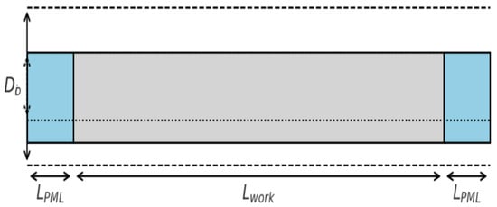
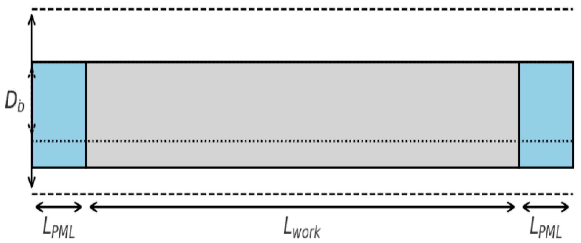
The finite element model (Figure 1) of a hollow steel pipe was constructed in Abaqus/CAE to simulate guided wave propagation. The pipe geometry was defined with an outer diameter = 219 mm, an inner diameter = 207 mm wall thickness d = 6 mm and a total length L = 3000 mm. To suppress boundary reflections, perfectly matched layer (PML) regions of LPML = 300 mm were attached to both ends, leaving an effective working section of = 2400 mm.
Figure 1.
Finite element model of the steel pipe.
Material properties were assigned as isotropic steel with E = 210 GPa, ν = 0.30, and ρ = 7850 kg/m3. From these parameters, the longitudinal and shear wave velocities were determined as
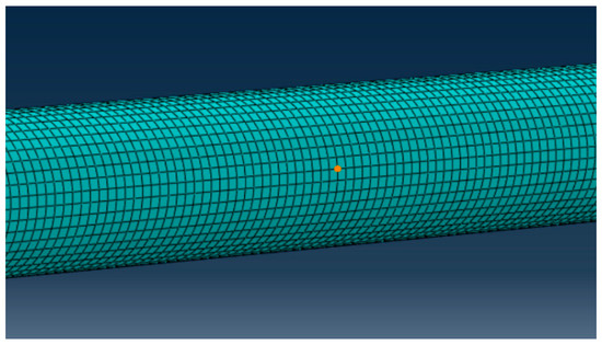
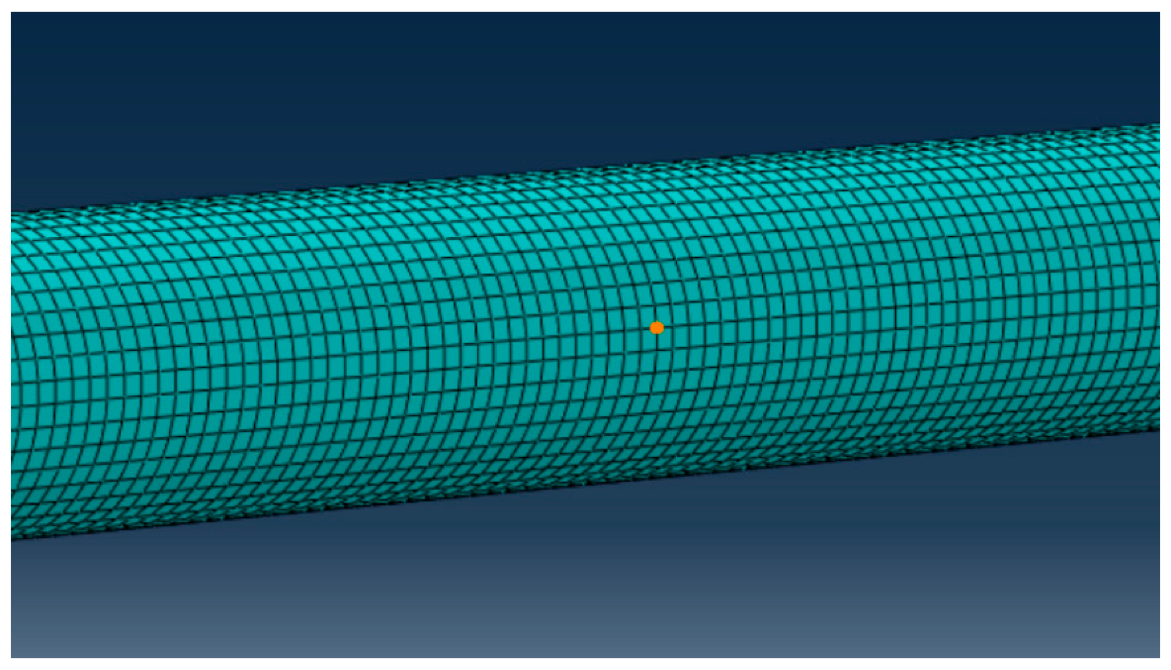
The pipe domain was discretized using eight-node reduced-integration brick elements (C3D8R). The mesh density was determined based on the wavelength-resolution criterion
where responds to the shortest wavelength associated with the highest excitation frequency nominal element size of approximately 2 mm was employed, ensuring at least four elements through the thickness to accurately capture radial displacement gradients and multi-modal wave behavior.
As shown in Figure 1, to prevent numerical artifacts, mesh compatibility was maintained between the perfectly matched layer (PML) region and the physical domain, thereby minimizing spurious reflections at the interface.
The PML regions were implemented by introducing gradually increasing damping along the axial direction, expressed as
which ensures exponential decay of outgoing waves and minimizes back-reflection into the computational domain. This configuration enables accurate simulation of wave propagation within the working section across the frequency range of interest (40–80 kHz).
The pipe geometry consists of an outer diameter , a wall thickness , and an effective working section of Perfectly matched layers (PMLs) of length are placed at both ends to absorb outgoing guided waves and eliminate artificial reflections at the model boundaries, the experimental setup is presented in Figure 2.
Figure 2.
Mesh discretization of the finite element model of the steel pipe.
To evaluate the robustness and resolution of the proposed imaging framework under different frequency conditions, a synthetic dataset was constructed that incorporates multi-frequency excitation, additive noise, and defect-induced scattering effects. The effective propagation distance of the pipe is set to , with a dominant group velocity of approximately 5 km/s.
Four central excitation frequencies—40, 50, 63, and 80 kHz—were selected to cover a representative range of frequency–thickness products, enabling a comparative analysis of long-range low-frequency propagation versus enhanced high-frequency scattering sensitivity. The frequency of 63 kHz is not selected as a unique or optimal value, but rather as a representative intermediate frequency within the investigated band. In practice, guided-wave imaging performance in this frequency range is not highly sensitive to small frequency variations (e.g., 60–65 kHz). Therefore, 63 kHz is chosen to characterize a typical frequency–thickness product between the lower-frequency (40–50 kHz) and higher-frequency (80 kHz) cases, without loss of generality.
A single axial crack is located along the centerline of the pipe. Its geometric dimensions produce an estimated increase in scattering-induced time-of-flight delay, corresponding to several microseconds. Gaussian white noise of approximately 20 dB SNR is added to emulate realistic sensor noise conditions. The sampling rate is 1 MHz with a window length of 0.5 ms (500 samples), sufficient to capture the excitation, forward propagation, scattered responses, and background noise.
The receiver array consists of 16 equally spaced sensors distributed circumferentially to acquire scattered signals from multiple angular positions. This configuration supports subsequent time-reversal (TR) focusing, topological derivative (TD) sensitivity mapping, and sparse Bayesian learning (SBL) inversion.
As shown in Table 1, these samples illustrate the multi-modal superposition and circumferential phase variation inherent in guided wave propagation.
Table 1.
Normalized time-domain samples of the received signals at sensors 1, 8, and 16 under 40 kHz excitation (first 10 sampling points).
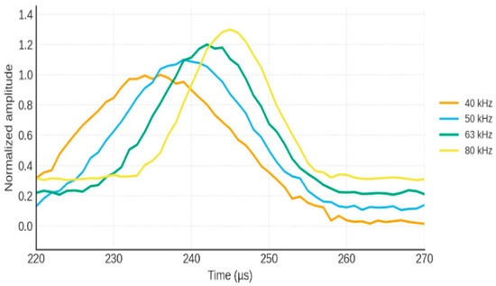
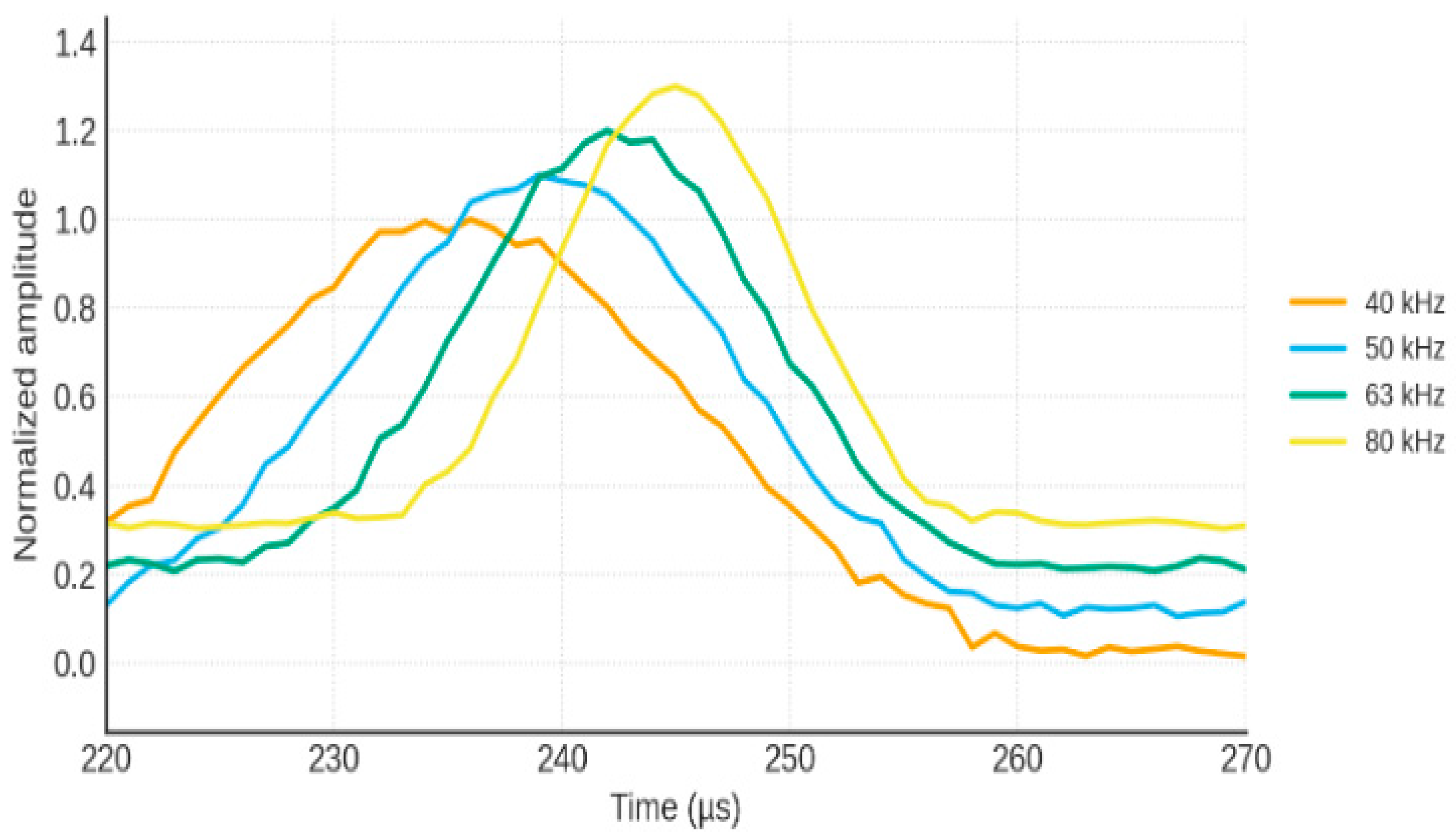
Figure 3 presents the time–frequency representation of the received guided-wave signals. These parameters highlight the complementary characteristics of multi-frequency guided waves: low-frequency components support long-range propagation with lower sensitivity, while high-frequency components exhibit stronger scattering but higher noise susceptibility.
Figure 3.
Time–frequency representation of received guided wave signals.
Table 2 Summary of signal characteristics at different excitation frequencies, including main peak amplitude, defect echo delay, scattering amplitude, and noise level.
Table 2.
Summary of extracted signal features at different excitation frequencies.
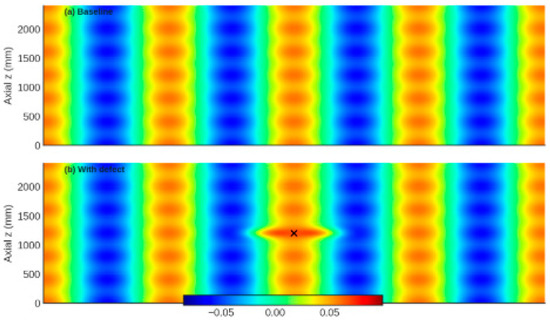
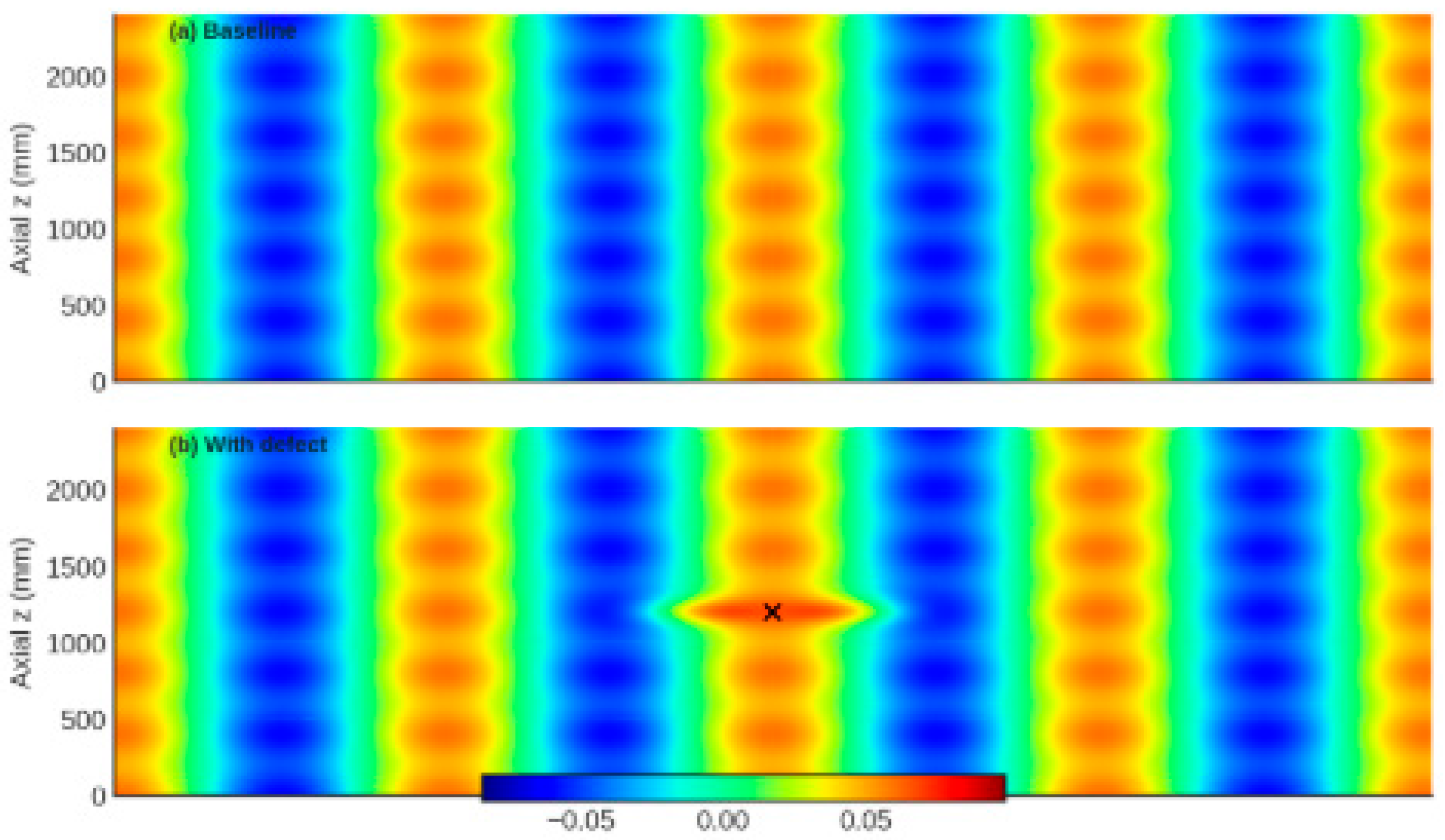
The spectrogram shows the dispersion-induced frequency-dependent group delay and the presence of scattered components at later times. Higher frequencies exhibit stronger scattering but shorter propagation distance, while lower frequencies maintain longer-range persistence but weaker sensitivity to small-scale defects. These characteristics justify the adoption of multi-frequency fusion in the proposed imaging framework (Figure 4).
Figure 4.
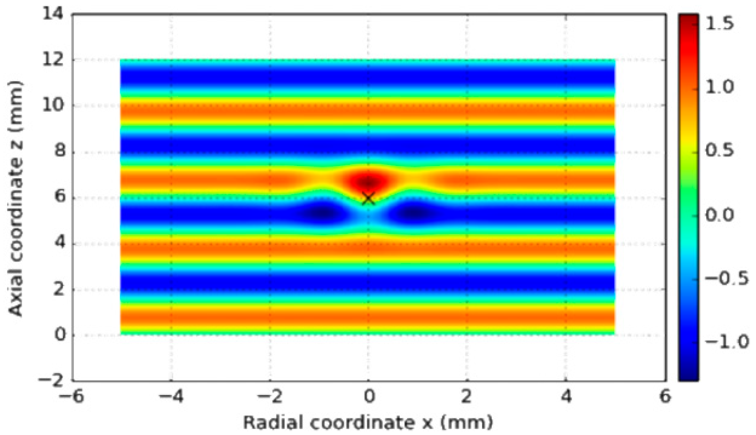
Comparison of guided wave fields obtained from finite element simulation. (a) Baseline wavefield in a defect-free pipe, showing smooth axial propagation and symmetrical modal distribution. (b) Wavefield in the presence of a single axial defect, exhibiting clear scattering, local amplitude perturbation, mode conversion, and perturbation of phase fronts near the defect region.
The scattering behavior of guided waves interacting with the defect is illustrated in Figure 5.The comparison highlights the sensitivity of guided waves to local stiffness discontinuities and provides the physical basis for time-reversal focusing, topological derivative sensitivity mapping, and sparse Bayesian inversion used in subsequent imaging sections.
Figure 5.
Guided wave scattering by a defect.
This schematic illustrates the incident guided wave, the interaction with a local defect, and the generation of scattered components. The scattered wavefronts contain defect-dependent features such as amplitude reduction, phase distortion, and mode conversion, which serve as essential information for TR focusing, TD sensitivity evaluation, and SBL-based probabilistic imaging.
4. Multi-Frequency Signal Processing and Imaging
This chapter presents the proposed multi-frequency guided-wave signal processing and imaging framework for defect detection in steel pipes. The framework integrates dispersion compensation, time-reversal (TR) imaging, topological derivative (TD) sensitivity analysis, sparse Bayesian learning (SBL)-based probabilistic inversion, and uncertainty modeling via domain randomization, forming a unified and physics-guided imaging scheme. The overall objective is to achieve robust and high-resolution defect localization under multimodal propagation, dispersion effects, and noise contamination.
For clarity, the complete algorithmic workflow of the proposed method is outlined here before detailing each individual component. Guided-wave signals are first excited and acquired at multiple central frequencies using a circumferential sensor array. For each frequency, dispersion characteristics are computed using the semi-analytical finite element (SAFE) method, and dispersion compensation is applied to correct waveform distortion caused by frequency-dependent group velocity variations. Single-frequency time-reversal imaging is then performed to refocus scattered wave energy and generate frequency-dependent TR images. These images are normalized and fused across frequencies to enhance spatial consistency and suppress single-frequency artifacts. In parallel, a topological derivative sensitivity analysis is conducted to construct a global physics-based map highlighting potential defect regions, which is subsequently combined with the TR result to form a hybrid TR–TD image. This fused image is further incorporated into a sparse Bayesian learning framework, where the posterior mean provides a probabilistic defect image and the posterior variance enables pixel-wise uncertainty quantification. Finally, domain randomization is employed during data generation and evaluation to assess the robustness of the proposed framework against uncertainties in material properties, boundary conditions, and noise levels.
Guided-wave propagation in steel pipes is inherently multimodal and strongly dispersive, particularly at medium-to-high frequencies and for flexural modes. The group velocity varies significantly with frequency, resulting in waveform distortion, pulse broadening, and energy smearing, which severely degrade the identifiability of weak defect echoes. To mitigate these effects and restore consistent time-domain signal characteristics across frequencies, dispersion compensation is applied as a prerequisite step prior to imaging. The dispersion relation is first obtained using the semi-analytical finite element (SAFE) method. For a given frequency , SAFE provides the corresponding wavenumber , from which the phase and group velocities are computed as
In the frequency domain, the guided wave signal at a given receiver can be expressed as
where and denote the amplitude and phase, respectively. The core idea of dispersion compensation is to construct a corrective phase term based on the SAFE dispersion relation, namely
where is the propagation distance between excitation and reception. A dispersion-compensated spectrum is then obtained by
After inverse Fourier transformation, the compensated time-domain signal exhibits a much narrower wave packet with reduced dispersion-induced spread. This pre-processing step significantly enhances the temporal resolution and improves the separation of overlapping echoes.
To further suppress group-velocity dispersion and restore a compact wave packet, a time-axis reshaping strategy is adopted. Given the group velocity function , the frequency-dependent travel time can be written as
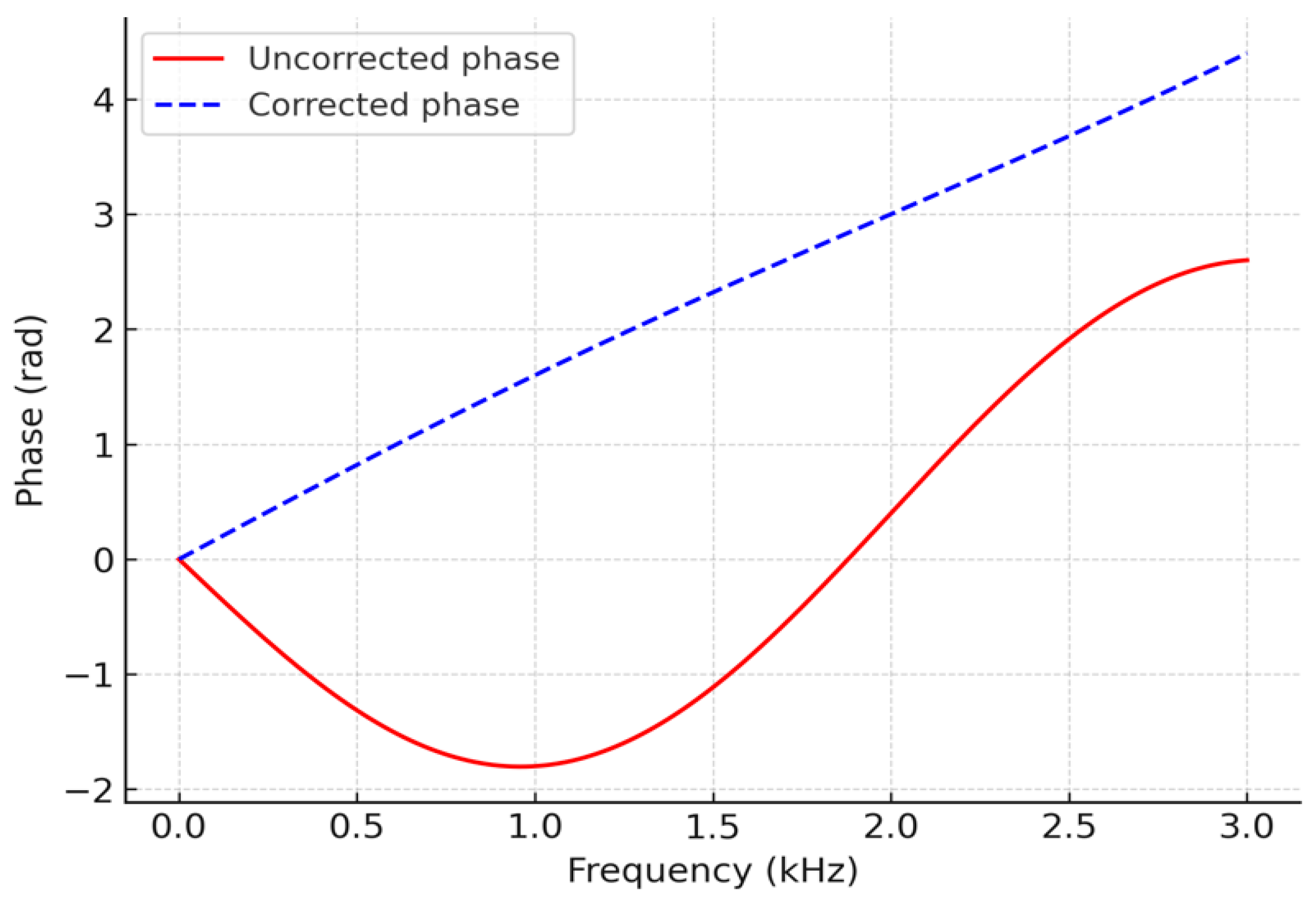
By mapping each frequency component from the original time axis to the corrected travel-time axis , the frequency components are aligned in time, effectively reshaping the dispersed waveform into a quasi-non-dispersive pulse. In addition, phase linearization is applied to ensure that the compensated phase–frequency relation is approximately linear, i.e.,
where is a reference travel time. After this transformation, the main lobe of the wave packet re-converges around , and the defect echo becomes more localized and easier to identify in the time domain.
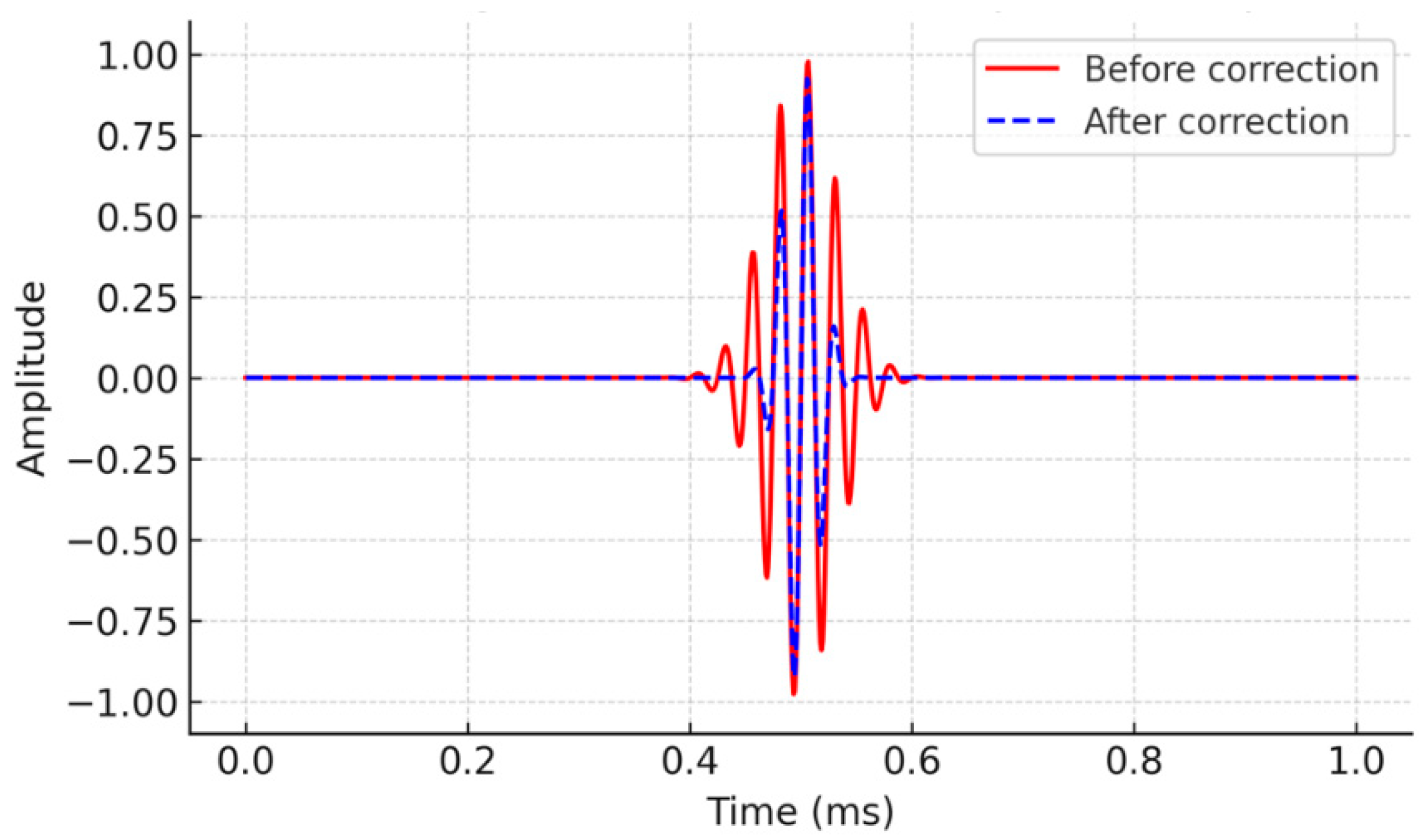
The upper panel shows the raw dispersed signal with evident pulse broadening and phase distortion. The lower panel presents the compensated signal, where the waveform is re-focused and the main peak is clearly sharpened.
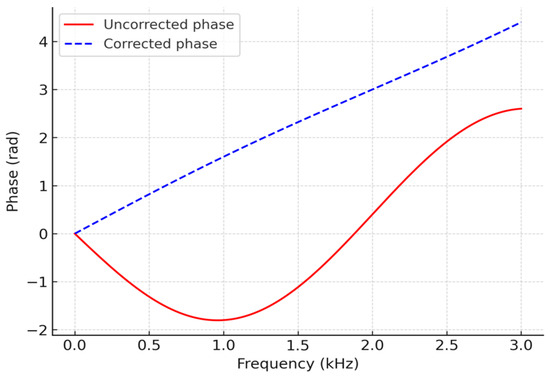
The effectiveness of the dispersion compensation is demonstrated by the comparison shown in Figure 6. The red solid curve denotes the original phase response, exhibiting strong nonlinearity with respect to frequency. The blue dashed line represents the compensated phase, which varies approximately linearly with frequency and guarantees time-domain focusing of the wave packet. Figure 7 provides an illustration of the phase-spectrum linearization process.
Figure 6.
Comparison of time-domain guided wave signals before and after dispersion compensation.
Figure 7.
Illustration of phase spectrum linearization.
After dispersion compensation, imaging is performed by combining multi-frequency time-reversal focusing and topological derivative-based sensitivity mapping. Single imaging methodologies are often limited by noise, modal interference, and false alarms. To overcome these limitations, a hybrid imaging framework is proposed that jointly exploits the strong spatial focusing capability of TR and the global sensitivity information provided by TD, thereby achieving accurate and low–false-alarm defect localization.
For a given frequency , let denote the dispersion-compensated guided wave signal recorded at receiver position . The time-reversed signal is back-propagated into the medium to obtain the reconstructed wavefield
where is the Green’s function and denotes the receiver aperture. Due to time-reversal invariance and reciprocity, scattered energy is concentrated at the original defect locations when . To enhance robustness, TR imaging is performed at multiple excitation frequencies (e.g., 40, 50, 63, and 80 kHz), and the corresponding focusing images are combined as
In this study, all single-frequency TR images are first normalized to unit energy to eliminate amplitude bias among different frequencies. Equal or mildly frequency-dependent weighting factors are then applied for multi-frequency fusion, where denotes the weight associated with the i-th excitation frequency. Numerical tests indicate that the proposed imaging results are not highly sensitive to moderate variations of , demonstrating the robustness of the multi-frequency TR fusion strategy. By integrating complementary information from different frequencies, this approach effectively reduces sensitivity to single-frequency artifacts and improves the stability of defect focusing.
The topological derivative provides a sensitivity measure of a chosen objective functional with respect to the nucleation of an infinitesimal defect at point (x). In a simplified form, the TD distribution can be written as
where and denote the forward and adjoint fields, respectively, and “:” denotes the double inner product of tensors. The TD map offers a global indication of potential defect regions but usually exhibits blurred boundaries and relatively high false-alarm rates. To leverage the complementary strengths of TR and TD, the TD sensitivity map is incorporated as a spatial prior for TR imaging. After normalization of the TD field, a fusion image is constructed as
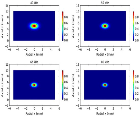
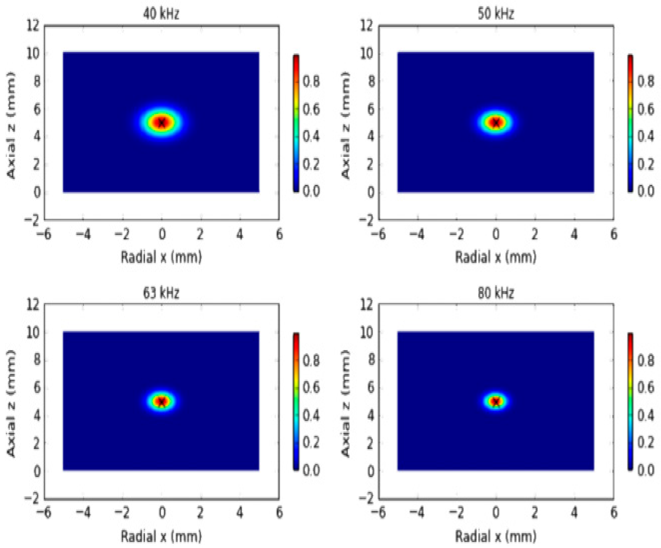
The fusion parameter is introduced to balance the contributions of time-reversal focusing and the TD-based sensitivity prior. Its value is selected based on robustness considerations rather than strict optimization, such that neither component dominates the fused image after normalization. Numerical results indicate that the proposed imaging performance is not highly sensitive to moderate variations of , demonstrating the stability of the fusion strategy. By appropriately weighting the TR and TD contributions, the proposed approach combines the high spatial resolution of TR imaging with the global physical consistency provided by the TD map.where is the normalized TD distribution and is a fusion factor. This hybrid strategy uses TR to achieve sharp spatial focusing while exploiting TD to suppress spurious maxima outside physically plausible defect regions, thereby effectively reducing false alarms and improving localization accuracy. Figure 8 compares the time-reversal focusing images obtained at different excitation frequencies.
Figure 8.
Comparison of time-reversal focusing images at different excitation frequencies.
The selection of the operating frequency range is guided by a quantitative trade-off between spatial resolution and noise robustness. In guided-wave imaging, the achievable spatial resolution is approximately proportional to half of the effective wavelength, i.e., Δx ≈ λ/2, where λ is determined by the phase velocity and excitation frequency of the dominant propagating mode. Higher frequencies yield shorter wavelengths and therefore improve imaging resolution, but they also suffer from increased attenuation, stronger modal dispersion, and higher sensitivity to measurement noise. Conversely, lower frequencies provide improved signal-to-noise ratio and longer propagation distance at the expense of reduced spatial resolution.
Based on the dispersion characteristics obtained from SAFE analysis and the geometric dimensions of the pipe, the frequency range of 40–80 kHz was selected as a compromise region where the dominant guided-wave modes remain well separated and exhibit moderate dispersion. The intermediate frequency of 63 kHz represents a typical frequency–thickness product within this range and is not intended to be a unique optimal value. By combining multiple frequencies spanning this band, the proposed multi-frequency fusion strategy effectively balances resolution enhancement and noise suppression, while reducing the sensitivity to frequency-dependent artifacts.
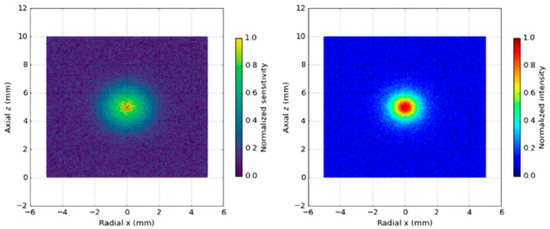
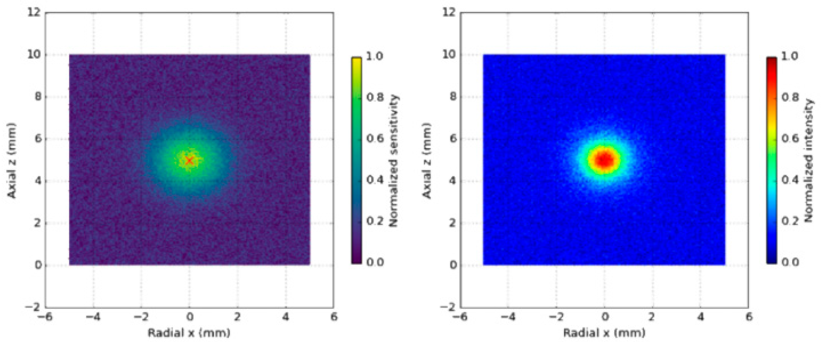
As shown in Figure 9, the TD sensitivity map and the TR–TD fusion imaging results exhibit distinct spatial characteristics. The left panel shows the TD-based sensitivity map, which provides global prior information on possible defect locations but suffers from noise and false alarms. The right panel presents the fused TR–TD image, where the combination of TR focusing and TD prior significantly reduces false alarms and enhances defect localization accuracy.
Figure 9.
Comparison between TD sensitivity distribution and TR–TD fusion imaging.
On top of TR–TD fusion, sparse Bayesian learning (SBL) is employed to perform probabilistic inversion of the defect distribution, enabling both high-resolution reconstruction and explicit uncertainty quantification. The guided wave imaging problem is discretized on a spatial grid and formulated as a linear inverse problem
where is the measurement vector, is the forward operator, represents the unknown defect distribution, and denotes additive noise. Typically , and the problem is severely ill-posed, requiring additional sparsity constraints.
Traditional deterministic sparse reconstruction can be formulated as
where denotes the components of in group , and is a regularization parameter. This optimization can be solved using fast iterative shrinkage-thresholding algorithms (FISTA), with per-iteration complexity and total complexity for iterations. However, such deterministic approaches do not provide uncertainty information and require manual tuning of .
To overcome these limitations, a hierarchical Bayesian model is adopted. The defect distribution is assumed to follow a zero-mean Gaussian prior
where are hyperparameters controlling sparsity at each spatial location. The hyperparameters are assigned Gamma priors
which promote sparsity by favoring small variance values. Under this hierarchical model and assuming Gaussian measurement noise with variance , the posterior distribution of is given by
where
and . Direct computation of has complexity , which is prohibitive for large-scale problems. In this work, the Woodbury matrix identity and parallel Cholesky factorization are used to reduce the complexity to approximately when , significantly improving computational efficiency.
The hyperparameters and noise variance are iteratively updated according to
Implementation details of the SBL framework are summarized as follows. A sparsity-promoting hierarchical Bayesian prior is adopted, where each imaging coefficient is modeled as a zero-mean Gaussian random variable with an individual variance governed by a Gamma hyperprior. This automatic relevance determination (ARD) mechanism enables the model to adaptively suppress irrelevant pixels and retain only statistically significant defect-related responses. The noise term is assumed to follow a zero-mean Gaussian distribution, which is consistent with the adopted simulation and data acquisition settings.
Model inference is performed by iteratively updating the posterior statistics and hyperparameters until convergence. In this study, convergence is declared when the relative change in the estimated hyperparameters or the log-marginal likelihood falls below a prescribed threshold, or when a maximum number of iterations is reached. Numerical experiments indicate that stable solutions are typically obtained within a limited number of iterations.
From a computational perspective, the dominant cost of the SBL algorithm arises from matrix operations associated with posterior updates, which scale polynomially with the number of imaging pixels and sensors. Since the SBL reconstruction is applied as a post-processing step after TR–TD fusion and the imaging grid size is moderate, the overall computational cost remains tractable for offline pipeline inspection and analysis.
Until convergence. In practice, 20–50 iterations are sufficient. For typical problem sizes , , the computational cost per frequency is on the order of floating-point operations, and the algorithm converges within a few seconds with GPU acceleration. A warm-start strategy is used in the multi-frequency setting: the SBL solution at a lower frequency is used as the initialization for higher-frequency inversions. This reduces the number of iterations required at higher frequencies by approximately 30–40%, effectively lowering the total computational burden across multiple frequencies.
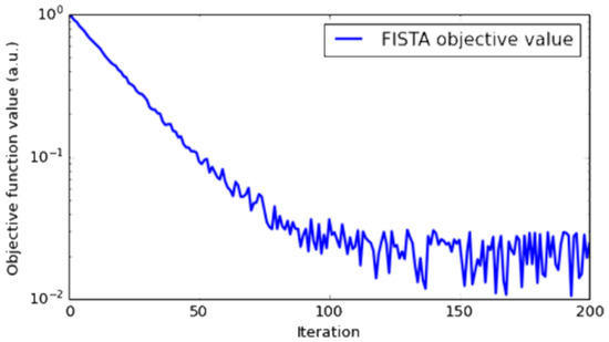
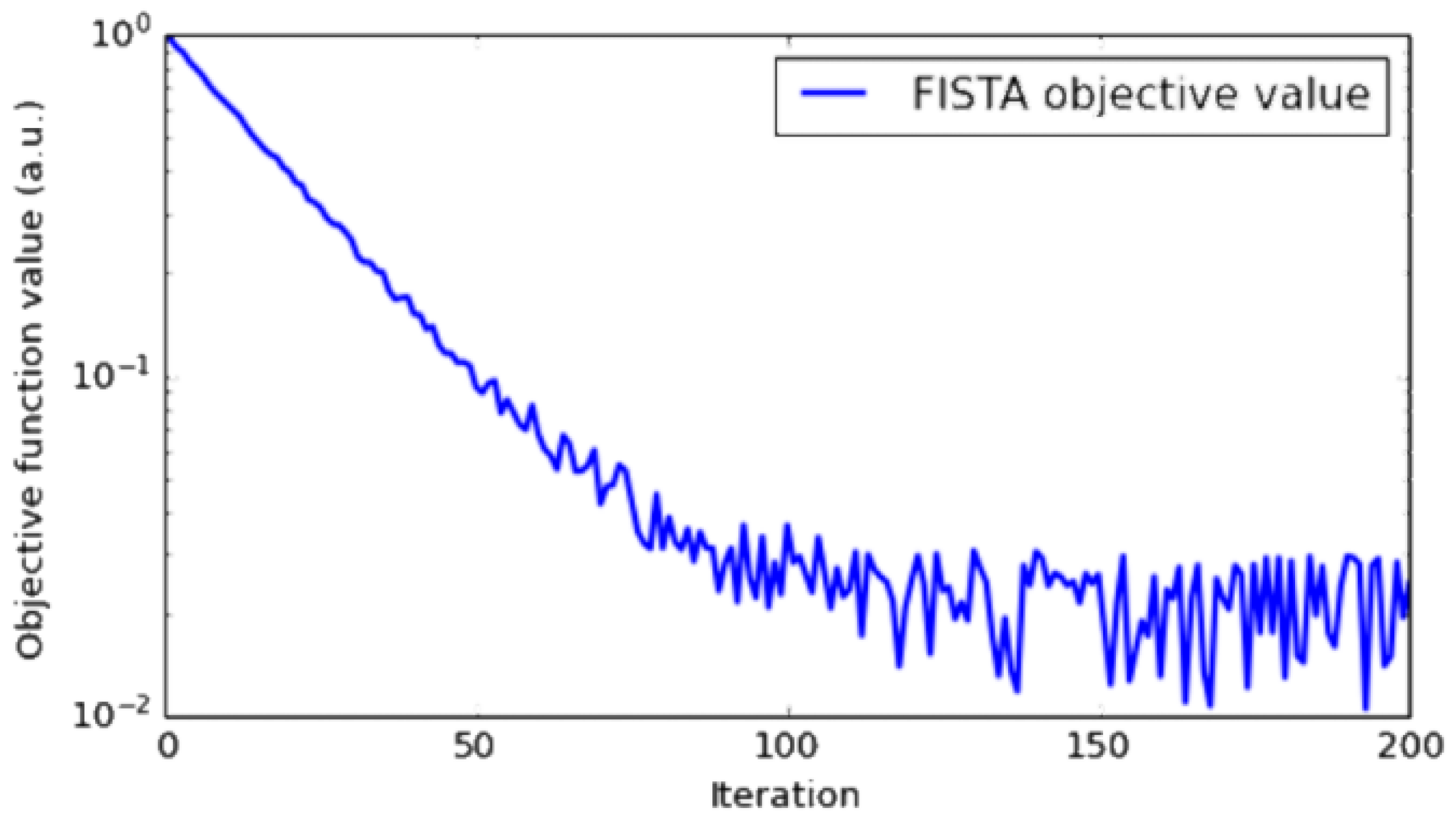
The posterior mean provides the optimal estimate of the defect distribution, while the diagonal of yields pixel-wise uncertainty. The resulting probabilistic images thus contain both spatial localization information and quantitative confidence levels, which are crucial for reducing false positives and supporting reliable decision-making. The adopted SBL formulation promotes sparsity and is particularly effective for localized defects such as cracks or small wall thinning, which are the primary focus of this study. For extended or distributed defects, including large-area corrosion or wear, the reconstructed image does not necessarily consist of isolated sparse peaks. Instead, it typically manifests as spatially continuous regions with elevated posterior probability, which still provides meaningful information regarding the defect extent and geometry. Moreover, the proposed framework is not fundamentally limited to strictly sparse representations and can be naturally extended to group-sparse or multi-scale Bayesian models to better characterize distributed damage patterns. The convergence behavior of the deterministic sparse reconstruction is shown in Figure 10. Such extensions, together with experimental validation on realistic corrosion scenarios, will be explored in future work.
Figure 10.
FISTA convergence curve for deterministic sparse reconstruction.
The objective function value decreases monotonically with iteration count and quickly reaches a plateau, demonstrating the fast convergence property in logarithmic scale.
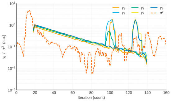
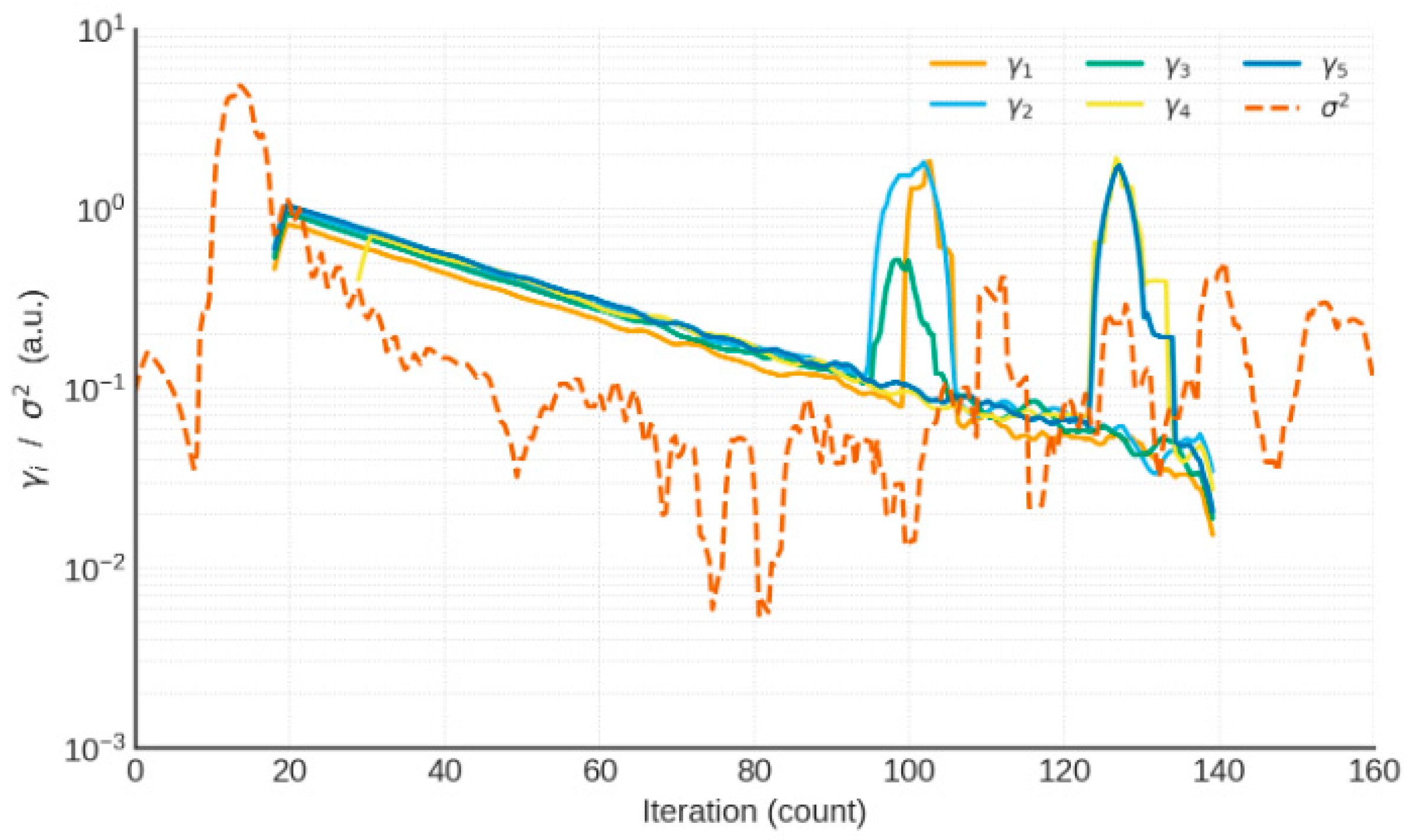
The Figure 11 shows five representative curves of (left axis, logarithmic scale) and the evolution of noise variance (right axis, dashed line), illustrating stable convergence of the hierarchical Bayesian updates.
Figure 11.
Convergence trajectories of SBL hyperparameters.
Finally, guided wave propagation and imaging performance are examined under various sources of uncertainty. Material and environmental uncertainties are modeled as random perturbations of elastic parameters:
where , , and are nominal values, and represent zero-mean Gaussian perturbations. For (5% variation), the perturbed phase velocity is
where is the nominal phase velocity. Monte Carlo simulations with Latin hypercube sampling are performed to obtain the statistical distribution of . For example, with frequency points and modes, each SAFE run requires on the order of FLOPs, and 1000 samples lead to a total cost of FLOPs, which can be completed in a few hours on a single GPU. The results show that the phase velocity of the mode is highly stable (<1%) drift, whereas the L(0,2) and low-order flexural modes may exhibit 5–8% drift, necessitating dispersion compensation to maintain imaging accuracy.
Domain randomization is further introduced at the modeling and data generation levels. Geometric perturbations include random crack lengths (20–80 mm), widths (0.5–2.0 mm), and random axial and circumferential positions. Boundary perturbations are modeled by varying the reflection coefficient of absorbing boundaries between 0 and 0.05. Signal-level perturbations encompass phase noise , amplitude fluctuations of ±10%, and bandwidth variations of ±5%. Multi-frequency data at 40, 50, 63, and 80 kHz are combined to build a training set of samples. Each sample requires one finite element simulation, with a typical element count of and computational cost on the order of FLOPs per simulation. With GPU-based parallelization, generating 5000 samples can be completed within approximately 12 h.
To quantitatively assess robustness, several evaluation metrics are defined. The imaging stability index (ISI) is given by
where and denote the mean and standard deviation of the imaging intensity at location (x) under random perturbations. The false positive rate (FPR) is defined as
where is the number of false-alarm pixels and is the total number of evaluated pixels. The localization error (LE) is measured by
where and are the estimated and true defect locations, respectively. These metrics provide a comprehensive assessment of robustness with respect to random variations in material properties, geometry, boundaries, and signal characteristics.
5. Numerical Simulation and Results Analysis
To systematically validate the applicability and robustness of the proposed multi-frequency guided wave imaging method, numerical simulations are carried out for representative defect scenarios in steel pipes, including a single crack defect and multiple or closely spaced defects. All simulations are based on the three-dimensional finite element model described earlier. The excitation is a Gaussian-modulated sinusoidal tone burst with central frequencies of 40, 50, 63, and 80 kHz. Perfectly matched layers (PMLs) are applied at both ends of the pipe to suppress unwanted reflections. The signal processing procedures considered include single-frequency time-reversal (TR) focusing, topological derivative (TD) sensitivity mapping, multi-frequency TR–TD fusion imaging, and sparse Bayesian learning (SBL)-based probabilistic imaging. Their performance is compared in terms of localization error (LE), false positive rate (FPR), and imaging stability index (ISI).
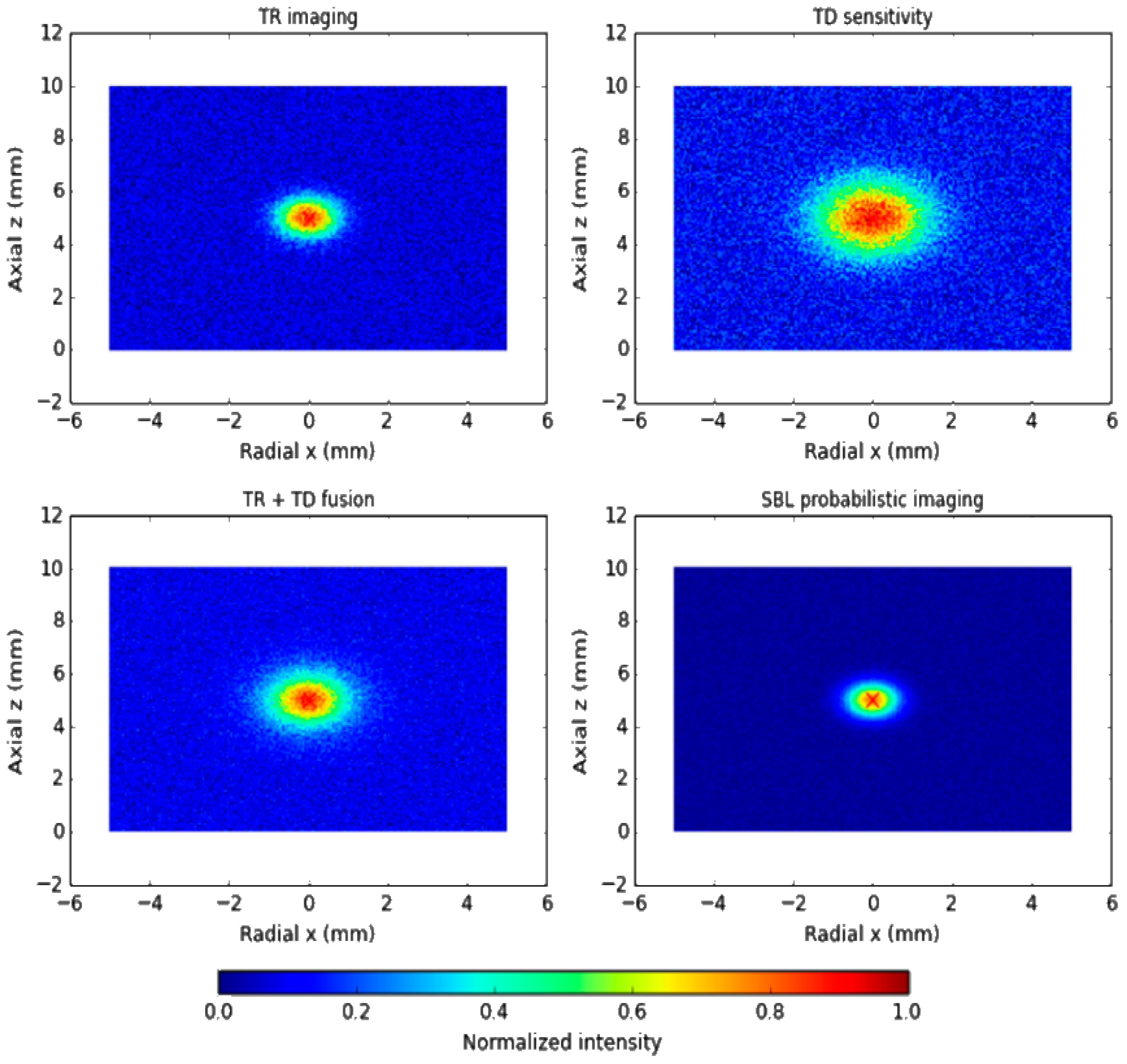
In the single-crack scenario, a longitudinal crack is introduced at the axial center of the pipe, with a length of 40 mm and a depth equal to 20% of the wall thickness. The simulation results show that single-frequency TR produces a focusing response at all tested frequencies. However, at lower frequencies the focal region is relatively diffuse and the localization accuracy is insufficient, whereas at higher frequencies (63–80 kHz) the focal peak becomes sharper and the localization error is reduced to within 2 mm. The TD-based image provides a global sensitivity distribution over the entire domain and indicates the vicinity of the defect, but it suffers from blurred boundaries and a significant number of false alarms. When TR and TD are fused, the focusing energy at the crack location is substantially enhanced and spurious maxima are effectively suppressed. Further improvement is achieved by applying SBL probabilistic imaging: the reconstruction not only accurately recovers the crack location and extent, but also yields a pixel-wise confidence map. The probability in the crack region exceeds 95%, whereas the background remains below 5%, indicating a clear separation between defective and defect-free areas and significantly enhanced reliability of the imaging result.
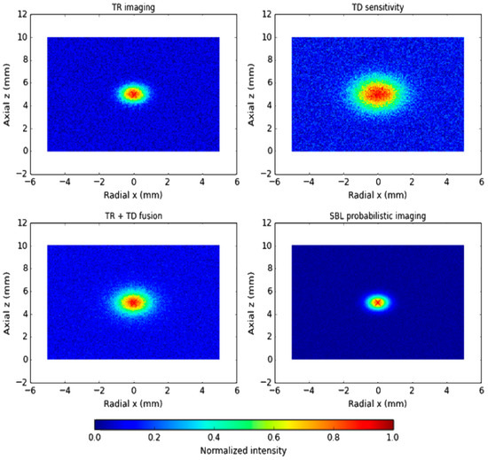
Figure 12 presents the TR imaging, TD sensitivity distribution, TR–TD fusion result, and the SBL probabilistic image for comparison. TR exhibits good focusing capability but is sensitive to frequency selection and noise; TD provides global sensitivity but shows many false alarms; the TR–TD fusion combines sharp focusing with global prior information and effectively suppresses spurious responses; SBL achieves the highest resolution and reliability, with crack-region probabilities greater than 95% and background probabilities below 5%.
Figure 12.
Imaging results for a single-crack defect.
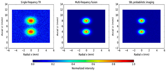
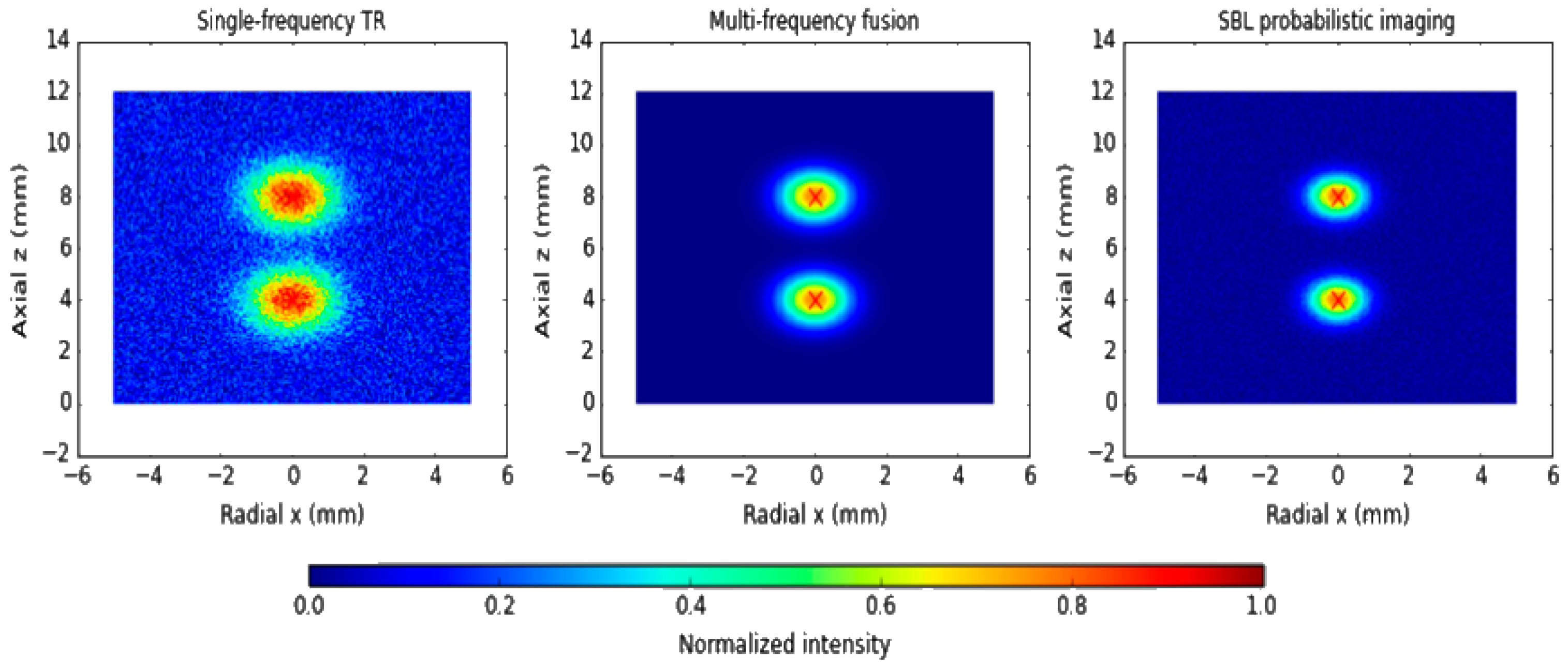
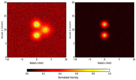
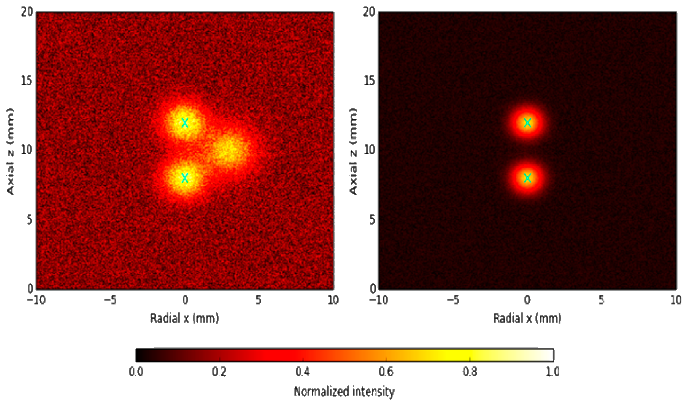
To examine the ability to resolve neighboring defects, a second scenario with two longitudinal cracks separated by 60 mm in the axial direction is considered. At low frequencies, single-frequency TR produces a single merged peak due to overlapping wavefields, making it difficult to distinguish the two cracks. At higher frequencies, the peaks become separable but the signal-to-noise ratio deteriorates and the results are more vulnerable to noise and modeling errors. Multi-frequency TR focusing, by contrast, clearly resolves the two defects with a localization error ≤ 3 mm. The TD map again identifies the general region of damage but exhibits fuzzy boundaries. The SBL reconstruction yields the best separation of neighboring defects, accurately resolving both cracks with confidence levels exceeding 90% and substantially mitigating modal interference and noise contamination.
For two cracks separated by 60 mm, single-frequency TR at low frequency fails to resolve the defects and yields a single broadened peak. Multi-frequency TR produces two distinguishable focal spots with improved stability, and SBL probabilistic imaging provides the clearest separation and the highest localization accuracy and confidence. Figure 13 illustrates the capability of imaging framework to resolve multiple and closely spaced defects.
Figure 13.
Imaging results for multiple and closely spaced defects.
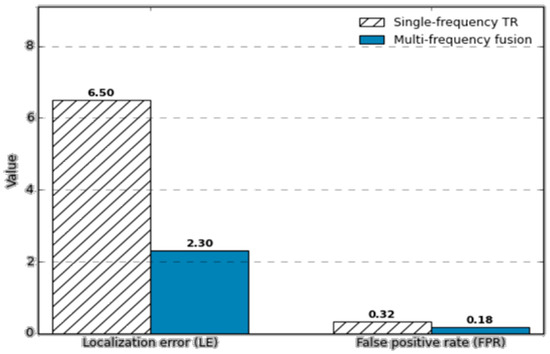
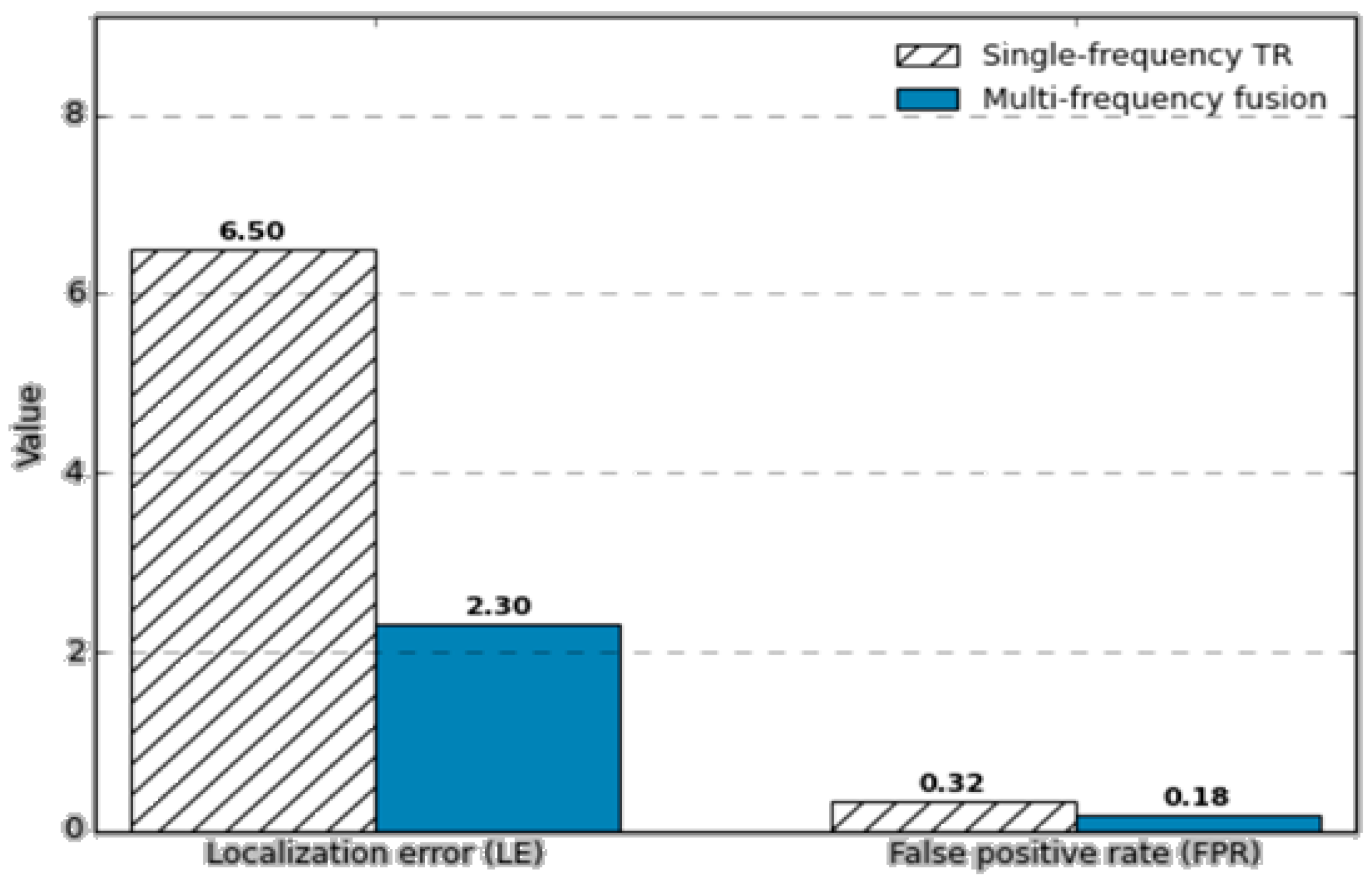
To quantitatively assess the benefit of multi-frequency fusion, imaging performance indicators are compared between single-frequency TR and multi-frequency methods. Numerical results show that the localization error decreases from 6.5 mm to 2.3 mm on average, and the false positive rate is reduced from 32% to 18% when multi-frequency TR–TD–SBL imaging is employed. For both single and multiple defect scenarios, the proposed method significantly improves accuracy and reduces false alarms, demonstrating superior performance over conventional single-frequency TR.
As shown in Figure 14, bar plots of localization error (LE) and false positive rate (FPR) show that multi-frequency TR–TD–SBL imaging substantially outperforms single-frequency TR, with LE reduced from 6.5 mm to 2.3 mm and FPR reduced from 32% to 18%.
Figure 14.
Imaging performance comparison under multi-frequency fusion.
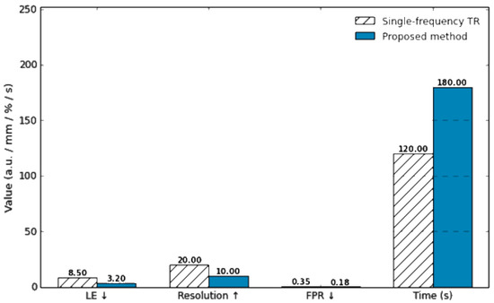
To further evaluate the advantages of the proposed imaging framework, a systematic comparison is conducted against conventional single-frequency TR. In the single-crack case, single-frequency TR at low frequency exhibits a localization bias exceeding 5 mm and a wide focal spot, indicating limited resolution. At higher frequencies, the resolution improves, but the signal-to-noise ratio decreases and the method becomes more sensitive to noise and modeling uncertainties. In contrast, the proposed multi-frequency TR–TD fusion effectively mitigates dispersion effects and yields localization errors below 2 mm. When combined with SBL probabilistic imaging, the crack geometry is clearly reconstructed and complemented by confidence level information, facilitating more reliable interpretation. In the multiple-defect case, single-frequency TR at low frequency fails to distinguish two cracks separated by 60 mm, whereas high-frequency TR can partially resolve them but still suffers from significant localization errors and false alarms. The proposed approach, which integrates multi-frequency fusion and SBL sparse reconstruction, roughly doubles the effective resolution and reduces the false positive rate by about 40% compared to single-frequency TR.
From the computational perspective, the complexity of single-frequency TR is on the order of , where (M) and (N) denote the number of receivers and spatial grid points, and (T) is the number of time samples. The proposed Bayesian framework requires approximately operations due to the matrix inversions involved. However, by exploiting warm-start strategies and GPU-based parallel computing, the total computation time remains on the order of minutes, which is acceptable for offline inspection and condition assessment. Overall, the method trades a moderate increase in computational cost for substantially higher localization accuracy, improved resolution, and lower false positive rate, and thus clearly outperforms conventional TR imaging in comprehensive performance.
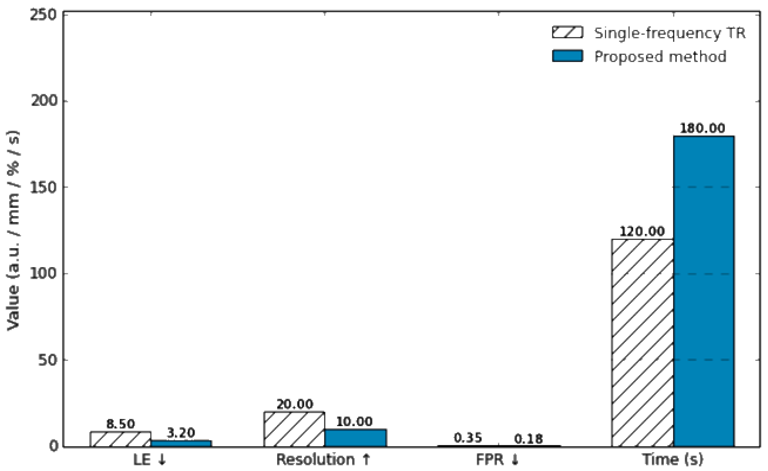
Figure 15 provides a quantitative performance comparison between the conventional single-frequency TR method and the proposed multi-frequency TR–TD–SBL approach. The bar chart summarizes localization error (LE), spatial resolution, false positive rate (FPR), and computation time. The proposed method achieves significantly lower LE and FPR and higher resolution, while keeping the computation time within a practical range through warm-start initialization and GPU acceleration.
Figure 15.
Quantitative performance comparison between conventional single-frequency TR and the proposed multi-frequency TR–TD–SBL method.
In practical engineering environments, guided wave signals are often affected by measurement noise, environmental vibrations, and modal coupling, which may obscure defect signatures or distort imaging results. To verify the robustness of the proposed method under such adverse conditions, additional numerical studies are carried out. First, noisy experiments with different signal-to-noise ratios (SNRs) are considered by adding zero-mean Gaussian white noise to the received signals.
It should be noted that Gaussian white noise is adopted here as a baseline noise model to enable controlled and reproducible numerical evaluation. In practical pipeline inspections, guided wave signals may also be affected by non-Gaussian and structured noise sources, such as pump-induced vibrations, flow turbulence, and environmental disturbances, which are not fully represented by the current simulation setting. The SNR is defined as
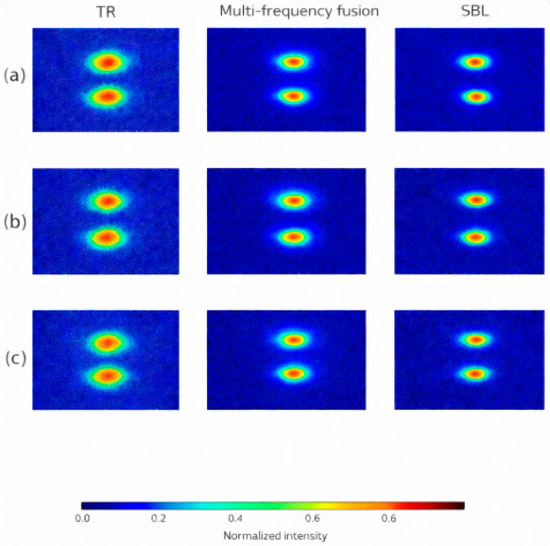
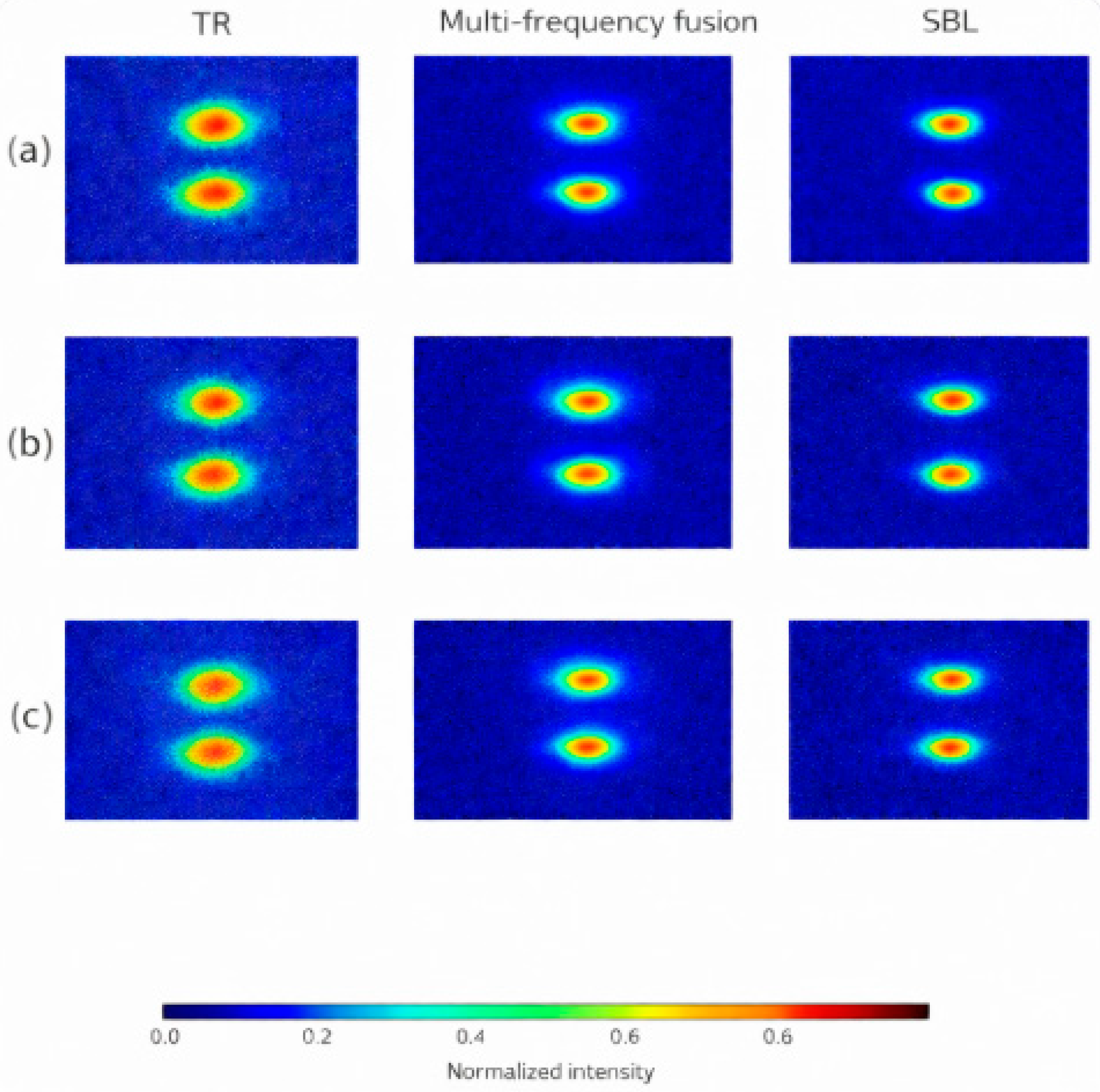
where and denote the signal and noise powers, respectively. Three typical SNR levels are studied: 20 dB, 10 dB, and 0 dB. At SNR = 20 dB, both TR and the proposed method produce clear focusing and accurately identify the crack location. At SNR = 10 dB, the TR image shows noticeable degradation and spurious peaks begin to appear, while the multi-frequency TR–TD–SBL approach still maintains a distinguishable focal spot with limited false alarms. At SNR = 0 dB, noise severely contaminates the signals, leading to blurred images and a substantial increase in false alarms for single-frequency TR. In contrast, the proposed method continues to highlight the true defect location, although with increased uncertainty, and keeps the overall false positive rate significantly lower than that of TR.
Figure 16 demonstrates the robustness of the proposed imaging method when subjected to different noise conditions. At 20 dB, defect focusing is clear; at 10 dB, the defect remains identifiable but mild false alarms appear; at 0 dB, single-frequency TR is heavily distorted by noise, whereas the proposed multi-frequency SBL-based imaging still indicates the correct defect location with reduced false positives.
Figure 16.
Imaging results under different noise levels. (a) SNR = 20 dB; (b) SNR = 10 dB; (c) SNR = 0 dB. Columns from left to right correspond to time-reversal (TR) imaging, multi-frequency fusion imaging, and sparse Bayesian learning (SBL) probabilistic imaging.
From an engineering perspective, the robustness of the proposed framework is evaluated under several representative sources of uncertainty commonly encountered in practical pipeline inspection. First, different defect scenarios, including variations in defect size, depth, and circumferential location, are considered to assess the stability of imaging performance with respect to defect characteristics. Second, measurement noise is explicitly introduced at different signal-to-noise ratio (SNR) levels, allowing a quantitative comparison of robustness among TR, TR–TD, and SBL-based imaging results. Third, uncertainties in pipe properties and inspection conditions are implicitly modeled through domain randomization, where material parameters, wave velocities, and boundary conditions are perturbed within realistic ranges. The consistent localization performance observed across these scenarios demonstrates that the proposed multi-frequency TR–TD–SBL framework exhibits strong robustness against noise contamination, defect variability, and modeling uncertainties, which are critical factors in real-world pipeline inspection.
In addition to noise, mode coupling is another major challenge in practical applications. At medium-to-high frequencies, different guided wave modes may exhibit closely spaced dispersion branches and exchange energy, resulting in mixed-mode signals at the receivers. To examine the performance under such conditions, a scenario involving strong coupling between the (L(0,2)) and (F(1,2)) modes is simulated. The results show that single-frequency TR in the mode-coupling region tends to generate spurious peaks and can produce localization errors exceeding 10 mm. By contrast, the multi-frequency TR–TD–SBL framework attenuates the influence of mode coupling, emphasizes the physically consistent defect signatures, and reduces the localization error to approximately 3 mm, with a marked reduction in false alarms.
The figure, presented in a C-scan–like format, contrasts single-frequency TR with the proposed method when the (L(0,2)) and (F(1,2)) modes are strongly coupled. Single-frequency TR exhibits ghost peaks and large localization bias, whereas the multi-frequency SBL-based imaging clearly identifies the true defect position with substantially fewer spurious responses.
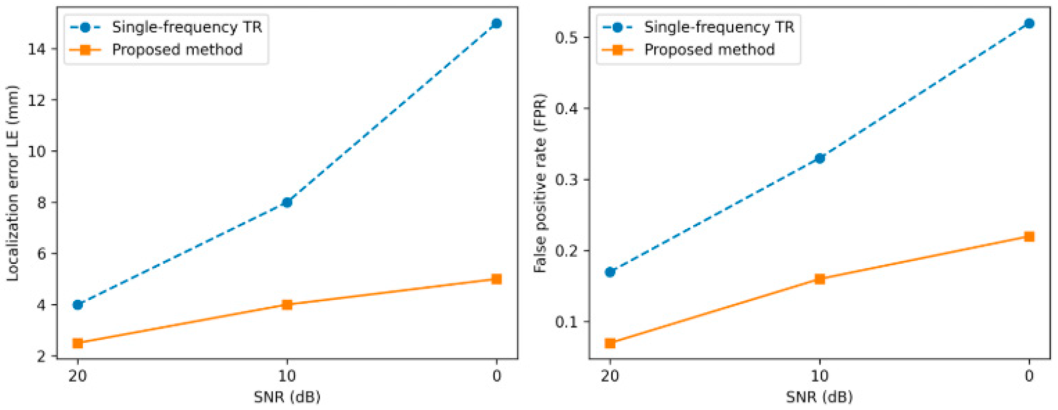
To quantitatively assess robustness with respect to noise and mode coupling, the dependence of localization error (LE) and false positive rate (FPR) on SNR is evaluated. As shown in Figure 17, the imaging performance is evaluated under the presence of mode-coupling effects. The SBL inversion yields a posterior distribution , where the mean vector represents the optimal estimate of the defect distribution and the diagonal entries characterize the variance (uncertainty) at each pixel. For the single-crack scenario, the probabilistic image shows defect-region probabilities exceeding 95%, whereas background pixels remain below 5%, forming a visually clear and statistically meaningful defect focus. The variance map reveals higher uncertainty along the crack boundary, reflecting lower confidence in the exact contour, while the crack interior exhibits lower variance and thus more reliable localization. Statistical analyses indicate that, at the 95% confidence level, the mean localization error of the proposed method is 2.8 mm, significantly lower than the 8.4 mm obtained with single-frequency TR. The false positive rate, when thresholded by uncertainty information, is reduced to about 12%, compared with 34% for the conventional method.
Figure 17.
Imaging comparison under mode-coupling conditions.
The curves of localization error (LE) and false positive rate (FPR) versus SNR show that the proposed multi-frequency SBL-based imaging consistently outperforms single-frequency TR across all noise levels. By incorporating posterior uncertainty, high-confidence regions are preserved while low-confidence artifacts are suppressed, leading to both lower LE and FPR and significantly enhanced stability and interpretability of the imaging results.
From a practical implementation perspective, several guidelines can be drawn for applying the proposed method in real-world pipeline inspection. Figure 18 illustrates how the robustness metrics evolve with different SNR levels, reflecting the stability of the proposed method. In terms of calibration, baseline signal acquisition on defect-free pipe sections can be used to compensate for systematic sensor and coupling variations, while time-of-flight alignment and amplitude normalization are recommended prior to multi-frequency fusion. For parameter tuning, the excitation frequency range can be selected based on dispersion analysis and inspection distance requirements, while the fusion weights and SBL hyperparameters may be chosen within moderate ranges, as the proposed framework exhibits low sensitivity to their exact values after normalization.
Figure 18.
Robustness metrics as functions of SNR.
Regarding system integration, the proposed approach is fully compatible with existing guided-wave inspection platforms employing circumferential transducer arrays, since it operates as a post-processing imaging framework without requiring hardware modification. Time-reversal focusing, TD sensitivity mapping, and SBL reconstruction can be implemented in software using the acquired multi-channel guided-wave data. Therefore, the proposed framework can be readily integrated into current nondestructive testing workflows, providing enhanced imaging resolution and reliability with limited additional computational overhead.
6. Conclusions
This study proposes a multi-frequency guided wave imaging framework for detecting and localizing defects in steel pipes, integrating time-reversal (TR) focusing, topological derivative (TD) sensitivity mapping, and sparse Bayesian learning (SBL). The method is developed to address key challenges in practical pipeline inspections, including dispersion, modal coupling, noise contamination, and the difficulty of resolving closely spaced defects. Comprehensive numerical simulations and robustness analyses validate the effectiveness and reliability of the proposed approach.
The results demonstrate that multi-frequency TR significantly enhances defect focusing by mitigating dispersion and improving spatial resolution compared with conventional single-frequency TR. The introduction of TD provides a physically interpretable global sensitivity distribution, serving as an effective prior for reducing false alarms. The integration of SBL further improves imaging accuracy by reconstructing sparse defect distributions while simultaneously quantifying uncertainty. The resulting probabilistic imaging maps provide pixel-wise confidence levels, enabling robust defect interpretation and suppressing low-confidence artifacts.
Extensive simulation studies—including single-crack, multiple-crack, low-SNR, and mode-coupling scenarios—show that the proposed method consistently achieves high localization accuracy, reduced false positive rate, and superior resolution. Quantitatively, the average localization error is reduced from 6.5 mm to 2.3 mm, and the false positive rate decreases from 32% to 18% under multi-frequency fusion. When combined with SBL, the method maintains defect-region probabilities above 95% and lowers the uncertainty-constrained false positive rate to approximately 12%. These improvements highlight the robustness of the approach under realistic engineering conditions.
Overall, the proposed TR–TD–SBL multi-frequency imaging framework provides a highly reliable, high-resolution, and computationally feasible solution for steel-pipe defect detection. It significantly outperforms traditional time-reversal imaging and demonstrates strong potential for deployment in long-range pipe inspection, structural health monitoring, and industrial nondestructive evaluation applications.
Future work will focus on extending the proposed framework to realistic non-Gaussian noise environments, including vibration-induced and flow-related disturbances, through experimental validation and advanced noise modeling strategies.
Author Contributions
Conceptualization, X.Z., C.H., Z.L. and S.W.; Methodology, X.Z., C.H. and S.W.; Formal analysis, X.Z., C.H. and Z.L.; Investigation, X.Z., C.H., Z.L. and S.W.; Resources, X.Z., Z.L. and S.W.; Data curation, X.Z., C.H. and S.W.; Writing—original draft, X.Z., C.H. and Z.L.; Writing—review & editing, X.Z., C.H., Z.L. and S.W.; Funding acquisition, X.Z., Z.L. and S.W. All authors have read and agreed to the published version of the manuscript.
Funding
This research was supported by the Inner Mongolia Natural Science Foundation, China, under Grant No. 2024LHMS06004 (2024–2026), entitled “Research on High-Order Helical Guided Wave Detection and Visualization Methods for Defects in Hydrogen Storage Cylinder Containers”, and by the Fundamental Research Funds for the Higher Education Institutions of Inner Mongolia Autonomous Region, China, under Grant No. 2024QNJS031 (2024–2025), entitled “Full-Wavefield Characterization and Damage Detection of Hydrogen Transmission Pipelines Using Single-Source Helical Guided Waves”. The Education Department of Inner Mongolia Autonomous Region, Graduate Scientific Research and Innovation Project, grant number KC2025064S. National Natural Science Foundation of China: Research on Defect Identification and Visualization of Pipelines under Complex Working Conditions Based on Ultrasonic Guided Waves and Structured-Light Vision, grant number 62161042.
Institutional Review Board Statement
Not applicable.
Informed Consent Statement
Not applicable.
Data Availability Statement
The raw data supporting the conclusions of this article will be made available by the authors on request.
Acknowledgments
The revised text now states that MATLAB (MathWorks, https://www.mathworks.com) was used for scientific plotting and data visualization during the preparation of this manuscript. No other external support or tools were involved.
Conflicts of Interest
The authors declare no conflict of interest.
Abbreviations
The following abbreviations are used in this manuscript:
| NDE | Nondestructive Evaluation |
| SHM | Structural Health Monitoring |
| TR | Time Reversal |
| TD | Topological Derivative |
| SBL | Sparse Bayesian Learning |
| SAFE | Semi-Analytical Finite Element |
| FEM | Finite Element Method |
| PML | Perfectly Matched Layer |
| DAS | Delay-and-Sum |
| FISTA | Fast Iterative Shrinkage-Thresholding Algorithm |
| SNR | Signal-to-Noise Ratio |
| LE | Localization Error |
| FPR | False Positive Rate |
| ISI | Imaging Stability Index |
| Probability Density Function | |
| MAP | Maximum A Posteriori |
| GPU | Graphics Processing Unit |
| FLOPs | Floating-Point Operations |
| C3D8R | Eight-Node Linear Brick Element with Reduced Integration |
| T(0,1) | Fundamental Torsional Guided Wave Mode |
| L(0,2) | Second-Order Longitudinal Guided Wave Mode |
| F(m,n) | Flexural Guided Wave Mode |
References
- Amaya-Gómez, R.; Sánchez-Silva, M.; Bastidas-Arteaga, E.; Schoefs, F.; Muñoz, F. Reliability assessments of corroded pipelines based on internal pressure—A review. Eng. Fail. Anal. 2019, 98, 190–214. [Google Scholar] [CrossRef] [Scilit]
- Xu, W.; Qiao, G.; Chen, X. Fatigue crack propagation behavior of steel pipelines. Int. J. Fatigue 2020, 132, 105382. [Google Scholar]
- Kishawy, H.A.; Gabbar, H.A. Review of pipeline integrity management practices. Int. J. Press. Vessels Pip. 2010, 87, 373–380. [Google Scholar] [CrossRef] [Scilit]
- Hopkins, P. Pipeline accident statistics and risk assessment. J. Loss Prev. Process Ind. 2016, 44, 575–586. [Google Scholar]
- Rose, J.L. Ultrasonic guided waves in structural health monitoring. Key Eng. Mater. 2004, 270–273, 14–21. [Google Scholar] [CrossRef] [Scilit]
- Cawley, P.; Alleyne, D. The use of guided waves for the inspection of long pipelines. NDT E Int. 1996, 29, 151–160. [Google Scholar]
- Raišutis, R.; Gribniak, V.; Jasiūnienė, E.; Samaitis, V. An inspection technique for steel pipe wall condition monitoring using ultrasonic guided waves. Sensors 2023, 23, 6812. [Google Scholar]
- Kwun, H.; Bartels, K.A. Magnetostrictive sensor technology and its application to guided wave inspection. Ultrasonics 1998, 36, 171–178. [Google Scholar] [CrossRef] [Scilit]
- Capineri, L.; Bulletti, A. Ultrasonic guided waves sensors and integrated structural health monitoring systems for impact detection and localization: A review. Sensors 2021, 21, 2929. [Google Scholar] [CrossRef] [Scilit]
- Zhang, X.; Lowe, M.J.S.; Cawley, P. Guided wave propagation and scattering at circumferential welds in pipelines. NDT E Int. 2020, 116, 102342. [Google Scholar]
- Lowe, M.J.S. Matrix techniques for modeling ultrasonic waves in multilayered media. IEEE Trans. Ultrason. Ferroelectr. Freq. Control 1995, 42, 525–542. [Google Scholar] [CrossRef] [Scilit]
- Hayashi, T.; Rose, J.L. Guided wave dispersion curves for a bar with an arbitrary cross-section. Ultrasonics 2003, 41, 175–183. [Google Scholar] [CrossRef] [Scilit]
- Su, Z.; Ye, L. Identification of Damage Using Lamb Waves; Springer: London, UK, 2009; pp. 1–346. [Google Scholar]
- Rasgado-Moreno, C.O.; Rist, M.; Land, R.; Ratassepp, M. Acoustic forward model for guided wave propagation and scattering in a pipe bend. Sensors 2022, 22, 486. [Google Scholar] [CrossRef] [Scilit] [PubMed]
- Liang, H.; Zhou, J.; Su, Z. Multi-frequency guided wave imaging under complex noise conditions. Mech. Syst. Signal Process. 2023, 188, 109971. [Google Scholar]
- Fink, M. Time-reversal acoustics. Phys. Today 1997, 50, 34–40. [Google Scholar] [CrossRef] [Scilit]
- Zang, X.; Zhang, Y.; Liu, H.; Chen, Z. Ultrasonic guided wave techniques and applications in pipeline defect detection: A review. Int. J. Press. Ves. Pip. 2023, 191, 105033. [Google Scholar] [CrossRef] [Scilit]
- Cawley, P. Guided waves in long-range nondestructive testing and structural health monitoring: Principles, history, and prospects. NDT E Int. 2023, 130, 102026. [Google Scholar] [CrossRef] [Scilit]
- Abuassal, A.; Al-Hussein, M.; Mustapha, S. A review of unidirectional ultrasonic guided waves: Principles, challenges, and perspectives. Sensors 2025, 25, 1050. [Google Scholar]
- Montaldo, G.; Tanter, M.; Fink, M. Time reversal of ultrasonic fields. IEEE Trans. Ultrason. Ferroelectr. Freq. Control 2004, 51, 1239–1248. [Google Scholar]
- Ing, R.K.; Fink, M. Time-reversed Lamb waves. IEEE Trans. Ultrason. Ferroelectr. Freq. Control 1998, 45, 1032–1043. [Google Scholar] [CrossRef]
- Bonnet, M. Topological sensitivity for 2-D and 3-D elastic problems. Int. J. Solids Struct. 2006, 43, 5561–5573. [Google Scholar]
- Feijóo, G.R. A new method in inverse scattering based on the topological derivative. Inverse Probl. 2004, 20, 1819–1840. [Google Scholar] [CrossRef] [Scilit]
- Hồ, T.L.; Bui, T.Q.; Zhang, C. Topology optimization for damage identification using guided waves. Mech. Syst. Signal Process. 2018, 99, 452–465. [Google Scholar]
- Etxaniz, J.; Aranguren, G.; Gil-García, J.M.; Sánchez, J.; Vivas, G.; González, J. Ultrasound-based structural health monitoring methodology employing active and passive techniques. Eng. Fail. Anal. 2023, 147, 107077. [Google Scholar] [CrossRef] [Scilit]
- Xu, B.; Su, Z. Multi-frequency guided wave imaging for damage detection. Smart Mater. Struct. 2014, 23, 045006. [Google Scholar]
- Gavric, L. Computation of propagative waves in free rail using a finite element technique. J. Sound Vib. 1995, 185, 531–543. [Google Scholar] [CrossRef] [Scilit]
- Tobin, J.; Fong, R.; Ray, A.; Schneider, J.; Zaremba, W.; Abbeel, P.; Levine, S. Domain randomization for transferring deep neural networks from simulation to the real world. In Proceedings of the IEEE/RSJ International Conference on Intelligent Robots and Systems, Vancouver, BC, Canada, 24–28 September 2017. [Google Scholar]

Disclaimer/Publisher’s Note: The statements, opinions and data contained in all publications are solely those of the individual author(s) and contributor(s) and not of MDPI and/or the editor(s). MDPI and/or the editor(s) disclaim responsibility for any injury to people or property resulting from any ideas, methods, instructions or products referred to in the content. |
© 2026 by the authors. Licensee MDPI, Basel, Switzerland. This article is an open access article distributed under the terms and conditions of the Creative Commons Attribution (CC BY) license.