Scheduling of the Automated Sub-Assembly Welding Line Based on Improved Two-Layer Fruit Fly Optimization Algorithm

Abstract

Faced with the contradiction between the increasingly growing demand and labor-intensive manufacturing modes, in the current era of rapid development of informatization and artificial intelligence, improving manufacturing efficiency by means of automated manufacturing equipment has become a recognized development direction for most shipyards. This trend is particularly evident in the manufacturing of sub-assemblies, which are the smallest composite units of the hull. Taking an automated sub-assembly welding line in a shipyard as the research object, this paper constructs a mathematical model aimed at optimizing production efficiency based on the analysis of its operational processes and characteristics and proposes an improved two-layer fruit fly optimization algorithm (ITLFOA) for solving the automated sub-assembly welding line scheduling problem (ASWLSP). The proposed ITLFOA features a two-layer nested algorithm structure, with several key improvements proposed for both optimization layers, such as heuristic rules for spatial layout, improved neighborhood operators, an added disturbance mechanism, and an added population diversity restoration mechanism. Finally, the performance of ITLFOA is validated through a comparative analysis against the initial two-layer fruit fly optimization algorithm (initial TLFOA), the well-established Variable Neighborhood Search (VNS) algorithm and the actual manual operation results on a specific case of a shipyard.

1. Introduction

In recent years, the demand for China’s shipbuilding industry has gradually increased. According to the latest data released by the China Association of the National Shipbuilding Industry, the number of new orders accounted for 64.2% of the global total, an increase of 15.1% compared with the last five years. China’s shipbuilding industry has maintained the world’s largest market share for 16 consecutive years [1].

However, most shipbuilding enterprises in China still rely on manual operations, which are time-consuming, labor-intensive, and inefficient. Moreover, the production and operational environment is harsh, facing hazards such as high temperatures, noise, and dust. The entire Chinese shipbuilding industry is confronted with the growing social problem of “labor shortage”.

To address the above issues, the state has actively advocated the implementation of an innovation-driven development strategy, promoting industrial upgrading through technological innovation, replacing old technologies with new ones, and substituting labor-intensive technologies with intelligent ones. Driven by Industry 4.0 and intelligent manufacturing, automated production lines have become the core carrier for transforming and upgrading the manufacturing industry for high-quality growth. In recent years, major domestic shipbuilding enterprises have responded to the national call and vigorously promoted the advancement and construction of “digital shipbuilding”.

Modern shipbuilding enterprises adopt a segmented production model based on group technology and are oriented towards intermediate products, which are gradually manufactured and integrated into ship products. As shown in Figure 1, the operation process of shipbuilding mainly includes component processing, component assembly and welding, block integration, and hull joining. All components formed in the process beginning with parts and ending at the complete hull are referred to as intermediate products, which are sequentially classified as sub-assembly, intermediate assembly, main assembly, and block. Sub-assemblies represent the smallest assembly units of a ship’s hull, and a typical ship is generally composed of tens of thousands of such sub-assemblies. Meanwhile, to adapt to the modern shipbuilding system, shipbuilding enterprises adopt a pull-type production planning and management system. Therefore, as the foundational and most granular assembly process in shipbuilding, sub-assembly manufacturing directly determines the dimensional accuracy, welding quality, and overall construction efficiency of subsequent intermediate and main assemblies. Smooth sub-assembly task performance underpins the steady advancement of subsequent works and on-schedule ship delivery.

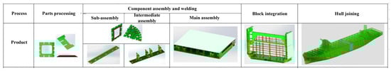
Figure 1. Shipbuilding process.

Furthermore, on the one hand, the number of sub-assemblies is enormous; an average ship consists of tens of thousands of sub-assemblies. On the other hand, most sub-assemblies weigh less than 1 ton. Although heavier than general products, they belong to the component level in the shipbuilding field and can be operated mechanically. Therefore, sub-assemblies have become the pilot target for shipyards to pursue automated transformation. At present, some shipyards have launched the construction of automated sub-assembly production lines, and studies on the manufacturing scheduling of automated sub-assembly production lines have become a top priority for current shipyard research. Therefore, this paper focuses on welding, the final production link of sub-assemblies, and investigates the scheduling problem of the automated sub-assembly welding line.

Some studies have already considered the scheduling problem of automated sub-assembly welding line [2]. But they focus on task sequencing optimization, typically assuming a known spatial layout and neglecting the impact of workpiece batching and layout on task allocation.

Compared with these existing works, the differentiated innovations of this study lie in two aspects. First, it expands the problem definition by establishing the first coupled model integrating sub-assembly batching, spatial layout planning, and multi-robot task allocation and sequencing. This approach breaks the limitations of single-dimensional optimization and enables the solution of complex scheduling problems with intertwined multi-constraints. Second, it achieves innovation in the algorithm framework: hierarchical heuristic rules and neighborhood operators are designed for the two-layer optimization structure, where outer-layer operators handle global adjustments of batching and layout and inner-layer operators adapt to local optimization of robot task allocation. This layered design circumvents the limitations of generic heuristic algorithms that adopt uniform optimization strategies for both global and local decision-making, effectively balancing the algorithm’s global exploration capability and local exploitation efficiency. It also ensures that the optimization process aligns with the inherent logic of the scheduling problem, laying a solid foundation for deriving high-quality and practical scheduling schemes.

The principal contributions of this work are outlined as follows.

1.

Makespan-minimized mathematical model tailored to the automated sub-assembly welding line scheduling problem (ASWLSP) in shipbuilding.

2.

Improved two-layer fruit fly optimization algorithm (ITLFOA) integrated with heuristic layout rules, optimized neighborhood operators, disturbance and diversity restoration mechanisms for hierarchical coordinated scheduling.

3.

Rigorous multi-benchmark comparative validation demonstrating ITLFOA superiority and extending resource-constrained scheduling algorithms’ applicability in ship robotic welding scenarios.

The remainder of this paper is organized as follows. Section 2 reviews related research on automated production line scheduling and ship sub-assembly scheduling. Section 3 introduces the automated sub-assembly welding line installed in the component workshop of a shipyard, analyzing its operational processes and characteristics. Based on this analysis, a mathematical model is established to minimize the total completion time. Section 4 describes the improved two-layer fruit fly optimization algorithm. Section 5 conducts performance verification using a specific case from the shipyard. Section 6 presents the conclusions.

2. Related Research

2.1. Scheduling for Automated Production Line

With the application of robots in manufacturing, extensive research has been conducted on their optimization scheduling.

(1) ASWLSP involving human labor

In some studies, it is referred to as the automation production line scheduling problem. However, the actual scheduling subject is still the operation itself, and robots are considered an important influencing factor. Shi et al. [3] developed a deep reinforcement learning-based intelligent scheduling method combined with discrete event simulation to address the defect of traditional methods in the automated production line scheduling that ignore the randomness of transportation units and processing times. Bai et al. [4] conducted research on the single-wafer cyclic scheduling problem in semiconductor manufacturing scenarios. With the goal of achieving the minimum achievable bound of cycle time. They constructed a system dynamic behavior model by extending the resource-oriented Petri Net and proposed a polynomial complexity algorithm. This algorithm realized the optimal setting of robot waiting time and buffer space configuration to achieve maximum production capacity with minimum buffer cost. Yang et al. [5] also conducted research on the single-wafer cyclic scheduling problem in semiconductor manufacturing scenarios. Considering tree-structured hybrid multi-cluster tools that including single-arm and dual-arm cluster tools, with the core goal of achieving optimal single-wafer cyclic scheduling, the setting of the robot waiting time is also one of the key paths to realizing the main objectives. Manzini et al. [6] proposed a predictive reactive scheduling method for process sequencing in automated assembly lines. This method balances the planning nature of predictive scheduling and the flexibility of reactive scheduling by predicting the uncertainty of processing times and dynamically adjusting the task allocation of shared resources to minimize the makespan.

(2) ASWLSP without human labor

In the study of the automation production line scheduling problem with robot job scheduling as the main point of focus, some researchers focused on a dual-gripper integrated flow shop scheduling problem. Composed of multiple processing machines and a material-handling robot, the dual fixture robot unit executes either loading or unloading tasks sequentially while accommodating two parts concurrently. Robotic flow shop scheduling where a dual-gripper robot conveys parts between machines is solved with makespan as the evaluation index. Sriskandarajah et al. [7] devised a tailored heuristic technique to address flow shop scheduling in dual-gripper robotic cells. Kim and Lee [8] proposed a reinforcement learning-based solution to the dual gripper robotic cells scheduling problem. The author considered processing machines and material handling robots, with a focus on obtaining robot task sequences as the solution. The goal is to shorten the completion time as much as possible. Subsequently, attempts were made to solve this problem using the deep Q-learning method [9], the hybrid method combining timed Petri Net (TPN) with dominance property-based optimal algorithm (DPOA) [10]. For the re-entrant hybrid flow shop joint scheduling problem incorporating a dual gripper, Wang et al. [11] constructed an optimization model with objectives of minimizing makespan and total delay, and devised a Q-learning-based DDPG algorithm. Mao et al. [12] proposed the job shop scheduling problem with a dual-gripper robot and no buffers (JSSP-DR). For the first time, two types of optimization models are constructed: the basic model that aims to minimize the makespan and the extended model that simultaneously minimizes makespan and robot energy consumption. Moreover, the corresponding mixed integer linear programming (MILP) models and improved simulated annealing (ISA) algorithms are proposed.

Nevertheless, the focus of these studies lies in developing large-scale scheduling strategies for multi-product robotic cells without product process route overlap. Therefore, to meet the growing demand for customization, flexible robotic production systems have been proposed and attracting attention, with research focusing on their scheduling problems [13,14,15,16]. In such systems, flexible robots can perform multiple types of operations and can execute specific tasks on different machines according to availability and scheduling requirements during production planning. However, the transportation constraints and buffer constraints for robots are overlooked in the existing research.

It is evident that the aforementioned studies have not considered the issue of robot operational interference, and their research objects are all serial manufacturing systems, which are not applicable to sub-assembly welding operations using batch production. Hofmann and Wenzel [17] explored the planning problem of robotic production lines. With the objective of minimizing the cycle time of robotic manufacturing systems, they proposed a mixed-integer programming model based on the periodic event scheduling problem (PESP) to address the spatial collision risks and cyclic scheduling challenges in multi-robot collaboration. Finally, they solved for the minimum cycle time T through binary search and validated the algorithm at a prototype station for automotive side component assembly. Subsequently, Helmberg et al. [18] expanded research to solve the robot collaborative scheduling problem given that the robot operation sequence and motion trajectory have been determined. However, the focus of their research is to enhance the reliability of industrial robotic system commissioning through validating robot programs and logic controller configurations rather than exploring approaches to optimize and schedule robot operations.

Overall, research on automated production line scheduling to date can be largely classified into two categories. One category takes operation scheduling as the core, with robots merely serving as important influencing factors. The other focuses on robot-centric scheduling, within which studies on single-robot operations, flexible robot operations, and multi-robot collaboration have been gradually carried out. However, most of the current research targets serial manufacturing systems, failing to fully consider robot operational interference, which thereby makes it difficult to apply to batch-produced sub-assembly welding operations.

2.2. Scheduling Problem of Sub-Assembly

The sub-assembly welding operations scheduling problem falls into the category of the resource constrained project scheduling problem [19]. During the optimal scheduling process, there is a need to consider the reasonable allocation of the start time of each operation, worker resources, and spatial resources. At present, most research in the field of ship manufacturing focuses on ship blocks as the research object, and research on the scheduling of sub-assembly welding tasks remains relatively scarce in the existing literature.

(1) Heuristic three-dimensional bin packing algorithm

In the ship block construction process, the main research focuses on how to schedule the operation sequence and spatial layout of each block under the condition of limited spatial resources in the block construction workshop to maximize the utilization rate of the workshop’s spatial resources while meeting the completion deadline requirements of each block. Lee et al. [20] first defined the spatial scheduling problem in the context of ship block construction in 1996. Based on Lozano-Pérez’s configuration space theory [21], they proposed four heuristic layout rules for spatial scheduling in ship block manufacturing; Koh et al. [22] put forward the largest contact area (LCA) spatial layout rule to solve the ship block-related spatial scheduling problem (SBSCP), building on the configuration space theory and the four layout rules proposed by Lee et al. [20]. Shin et al. [23] employed a differential evolution algorithm integrated with the bottom-left (BL) layout rule to address the SBSCP. Shang et al. [24] constructed a time- and space-constrained three-dimensional bin packing mathematical model for the SBSCP and proposed an optimal contact algorithm more suitable for dynamic processes; subsequently, the start time of each block was regarded as a variable and a genetic algorithm was utilized to sort and optimize the sequence of block construction activities. Ge & Wang [25] developed a standard-angle filling-based block layout rule and a block-priority-driven genetic algorithm to address the SBSCP.

For the above research methods, the basic principle is to substitute rectangles with convex polygons for representing object shapes, and the feasible space is acquired by determining the difference set between the site allocation space and the obstacle space. However, such methods require determining the obstacle space of all existing objects, resulting in a large computational load; in addition, it is quite difficult to achieve precise positioning of sub-assembly welding in the welding workshop, making this method unsuitable for sub-assembly welding scenarios.

(2) Spatiotemporal decomposition strategy

Therefore, many scholars have proposed a spatiotemporal decomposition strategy, dividing the spatial scheduling problem into two phases—spatial layout optimization and scheduling sequence determination—thereby reducing the difficulty of solving the problem. Kwon and Lee [26] first grouped blocks according to their urgency, followed by sorting the blocks within each group based on their earliest scheduled start time. Dixit et al. [27] comprehensively proposed a combined time-based and resource-based rule, considering both the criticality of time and resources. To overcome the shortcoming of genetic algorithms being prone to falling into local optima, Ge and Wang [28] combined genetic algorithms with ant colony algorithms to propose an improved genetic ant colony algorithm. By virtue of large-scale mutations, this algorithm allowed the population to escape local optimal solutions and, thereby, obtain the optimal scheduling sequence. Hu et al. [29] generated the initial solution following the “larger area first” rule and, subsequently, enhanced the initial solution via a simulated annealing algorithm.

In summary, the sub-assembly welding operation scheduling problem falls into the category of resource-constrained project scheduling problems, which requires the coordinated management of process time, labor resources, and spatial resources. However, relevant research in the field of ship manufacturing is relatively scarce. Existing studies mainly focus on the spatial scheduling of ship blocks, with research methods that include proposing various layout rules and algorithms based on configuration space theory, yet these suffer from drawbacks such as large computational loads and poor adaptability to welding scenarios. Another approach is the spatiotemporal decomposition strategy, which splits the problem into two phases: spatial layout optimization and scheduling sequence determination. While this strategy reduces the difficulty of solving the problem through grouping, sorting, hybrid algorithms, and other means, it still fails to specifically address the scheduling requirements of sub-assembly welding operations.

2.3. FOA-Based Scheduling Methods

To contextualize the proposed approach within the existing body of knowledge, this section synthesizes key studies on FOA-based scheduling across relevant domains, delineating their contributions and limitations.

(1) FOA-based scheduling in robotic production and spatial constraints scenarios

In robotic production line scheduling, Shen et al. [30] employed FOA for multi-objective path planning in welding robots, establishing a foundation for metaheuristic applications but lacking integration of task scheduling with resource coordination. Meng et al. [31] proposed a fuzzy FOA method for ship pipeline processing, offering insights for uncertain constraints but failing to address spatial interference and skill-matching in multi-robot welding.

For spatial and constrained scheduling, Han et al. [32] adapted FOA for blocking flow shop problems, extending its application to classical scheduling variants yet restricting their scope to single-objective optimization. Wang and Li [33] designed a hybrid FOA for vehicle routing, contributing to metaheuristic hybridization strategies but not accommodating the sequential dependency and dynamic resource allocation inherent in welding tasks.

(2) FOA-based scheduling in hierarchical and multi-objective optimization

Regarding hierarchical and multi-objective optimization, Shang et al. [34] integrated FOA with simulated annealing into a general multi-objective framework, providing theoretical support for balancing convergence and diversity but without domain-specific customization for welding. Wang and Zheng [35] developed a knowledge-guided FOA for multi-skill resource scheduling, addressing complex constraints but overlooking dynamic resource changes in welding scenarios. Ma et al. [36] applied FOA to discrete test point optimization, verifying its applicability to discrete problems but not incorporating manufacturing-specific quality constraints.

Collectively, these studies confirm the feasibility of FOA in manufacturing scheduling. However, notable research gaps persist, including insufficient adaptation of general algorithms to welding-specific attributes, a predominant focus on isolated sub-problems within domain research, and a weak connection between general scheduling theory and practical welding scenarios.

The existing literature has covered three core research domains. However, there are notable research gaps in the current body of knowledge. First, FOA has been widely applied in scheduling scenarios such as general flow shops and pipeline processing. But little research has focused on its application to task allocation for robotic welding in shipbuilding, with little targeted research on key issues, including multi-robot collaboration, multi-skill matching, and welding quality constraints. Second, the field of ship welding scheduling mainly adopts traditional optimization methods such as genetic algorithms and immune optimization. The discrete optimization advantages of FOA, which are fewer parameters and faster convergence, have not been fully utilized. Third, existing studies have not yet systematically integrated four core elements: shipbuilding scenario, robotic welding, task allocation, and FOA. This leads to inadequate alignment between algorithms and specific application contexts. This study aims to fill these research gaps. By customizing and adapting FOA for task allocation and efficient operation in shipbuilding robotic welding, it establishes an accurate alignment mechanism between the scenario and the algorithm. This helps improve the efficiency and flexibility of task allocation in this field.

3. Problem Description and Modeling

3.1. Problem Description and Analysis

Figure 2 shows an automated sub-assembly welding line built in the component workshop of a shipyard, which consists of four areas: a manual loading and assembly area, a to-be-welded workpiece buffer area, an automated welding area, and a repair and unloading area. At first, components are manually transported to assembly stations for assembly work. After assembly, the components are sequentially conveyed to buffer stations and welding stations via the roller table system, where robots automatically identify and weld them to form sub-assemblies. And then, the sub-assemblies are transported to repair and grinding stations through the roller table system. Eventually, the sub-assemblies after repair and grinding are moved out of the line by workers.

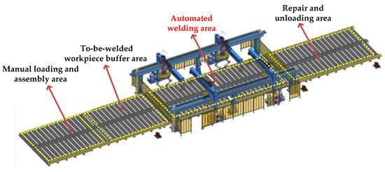
Figure 2. An automated sub-assembly welding line.

The robot system in the welding area consists of a cantilever device with $X/Y$-directional movement functions and a rotation function about the $\theta$-axis, as well as a robotic welding system. The robotic welding system is fixed within the cantilever device. Each cantilever device drives two robotic systems to move, and the two robots form a group and share all external axes, as shown in Figure 3. There are four sets of cantilever devices on both sides of the same track, meaning the entire production line is equipped with a total of eight robots.

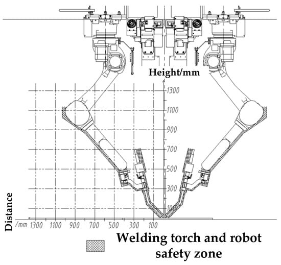
Figure 3. Schematic diagram of welding robot.

Based on their arrangement on both sides of the roller table, the four sets of cantilever systems can be divided into same-side cantilever systems and opposite-side cantilever systems. The same-side cantilever systems share a common track and can perform collaborative welding on workpieces within the welding reachable area along the track. Due to the limitations of arm span and track, the opposite-side cantilever systems can only handle welding tasks for workpieces within $3.5$ m in the Y-direction. It can be inferred that when welding workpieces with a width greater than $3.5$ m, the two sets of opposite-side cantilevers can collaborate on welding the workpiece. When welding workpieces with a width within $3.5$ m, the four sets of cantilever systems can be split into four independent cantilever welding systems for separate welding, and the entire production line can be divided into two independent upper and lower production lines for operation. The line is suitable for workpieces with a maximum height of 1 m and a maximum vertical welding height of 550 mm.

The x-axis of the sub-assembly workpiece coordinate system is arranged parallel to the length direction of the roller table. When the width of a workpiece perpendicular to the length direction of the roller table exceeds $3.5$ m, the welding tasks within $3.5$ m are performed by robots on the same side, while those beyond $3.5$ m are handled by robots on the opposite side. Therefore, when workpieces with a width exceeding $3.5$ m are placed in the welding area, the x-axis of their workpiece coordinate system must also be parallel to the length direction of the roller table. For workpieces with a width less than $3.5$ m, the x-axis of their workpiece coordinate system is usually placed parallel to the length direction of the roller table but can also be placed arbitrarily. In addition, the robot has a 200 mm margin in the width direction of the roller table (Y-direction), meaning that if the distance between the x-axis of the workpiece and the edge of the track is within 200 mm, the robot can compensate for it; otherwise, due to the arm span limitation, the robot cannot compensate for this distance deviation, resulting in a failure to perform the intended welding tasks.

In terms of collision prevention, the two sets of opposite-side cantilever systems cannot simultaneously weld tasks near the $3.5$ m centerline of the roller table. Usually, a safe distance must be maintained, or robot 1 performs welding while robot 2 pauses and waits until robot 1 completes welding and moves away from the centerline before robot 2 performs welding tasks near the centerline. For the two sets of same-side cantilever system welding workpieces on the roller table, the safe distance is defined as a spherical area with the center of the base of each cantilever system as the center and a radius of $3.5$ m. If the distance between the two systems is greater than this safe distance, no collision will occur. Therefore, for the two sets of same-side cantilever systems, there are two independent welding areas on both sides of the welding zone, in which welding tasks can only be welded by one cantilever welding system. In addition to the two independent welding areas on the same side, there is also an independent welding area, and the welds in it need to be assigned to two sets of cantilever welding systems.

3.2. Problem Formulation

Improving robot welding efficiency is the current main demand of enterprises, so this study takes minimizing the total completion time as the objective function. The analysis of the automated sub-assembly welding line reveals that sub-assemblies are placed in batches in the work area for welding. Therefore, it is initially essential to take into account the batching and spatial layout of sub-assemblies with various shapes. Subsequently, for batches of sub-assemblies, their welding tasks need to be assigned to four sets of cantilever welding robots, and their welding sequence must be determined in the limited work area, as shown in Figure 4. These four sets of cantilever welding robots could be deemed analogous to parallel processing machines, so this scheduling problem can be classified as the parallel machine scheduling problem. However, unlike traditional parallel machine scheduling problems, equipment interference between robots must be considered during the operation of the four parallel welding robots.

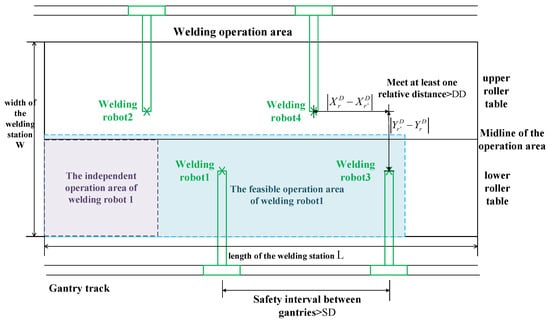
Figure 4. Schematic diagram of the work area.

The main decision variables of this scheduling problem include sub-assembly batching, sub-assembly spatial layout, welding task assignment within batches, and welding task sequencing within batches. Among these, welding task assignment and sequencing can only be further optimized after determining the sub-assembly sequencing, batching, and spatial layout, resulting in the nested optimization characteristic of this problem. In summary, the scheduling problem of the automated sub-assembly welding line studied in this paper can be defined as a two-layer cyclic optimization problem: first, the outer layer optimizes the sub-assembly sequencing, batching, and spatial layout. Then, the inner layer further optimizes the welding task assignment and sequencing. Finally, the solution of the outer layer optimization is further adjusted based on the results of the inner layer optimization.

To elucidate the modeling logic, a simplified illustrative example is considered. Suppose a batch contains several sub-assemblies of different shapes and sizes. The outer-layer optimization first determines (1) the sequence in which these sub-assemblies enter the welding area, (2) how they are grouped into batches for simultaneous processing, and (3) their precise spatial positions on the roller table to avoid physical overlap and respect robot reachability constraints. Once a feasible batch layout is fixed, the inner-layer optimization addresses the detailed scheduling within that batch: it assigns each individual welding seam task to one of the four robot systems and sequences the execution of these tasks on each robot, while strictly adhering to collision-avoidance constraints between the all robots. The overall makespan depends critically on both the outer layer and inner layer. The outer layer calculates an efficient spatial layout which maximizes parallel robot utilization. At the same time, the inner-layer carry out an optimal task assignment and sequence which minimize idle time and delays due to interference. This two-layer, cyclic approach reflects the practical nesting of these decisions in the operational control of the line.

3.2.1. Assumptions

(1) Once the spatial positions of sub-assemblies at the welding stations are determined, they will not be moved until the welding of the entire batch of sub-assemblies is completed. Most sub-assemblies require crane handling due to their weight, and adjusting their positions mid-welding would involve time-consuming crane operations and calibration, leading to prolonged downtime—this aligns with shipyard operational reality.

(2) The transfer time of sub-assembly batches into and out of the automated welding area is neglected in the model. Based on on-site data, the average transfer time is 30 s, accounting for only 0.67–1% of a batch’s completion time (3000–4500 s). This negligible proportion has minimal impact on scheduling accuracy, while simplifying the model to focus on core layout and task allocation.

(3) The idle movement time of welding robots between consecutive welding tasks is neglected in the model. Field measurements show the robot’s idle movement speed (0.13 m/s) is 20 times its welding speed, and each weld has a 90 s preparation time, resulting in idle movement time accounting for only 2% of total welding time. This simplification streamlines computation without affecting task sequencing or load balancing, as the time gap offers no practical decision-making value.

(4) When a welding task crosses the boundary between the upper and lower roller tables, take the lower roller table as an example. If the y-axis coordinate of the upper endpoint of the welding task is less than $W/2+MD$ but greater than $W/2$, the welding task can be completed by the robot in the next operation; If the y-axis coordinate of the upper endpoint of the welding task is greater than $W/2+MD$, the welding task is split into two tasks at the $W/2$ position, which are completed by the upper and lower robots, respectively. The same logic applies to the upper roller table. The splitting ensures full coverage of wide workpieces, avoids collision risks, and maintains welding efficiency, making the assumption highly applicable to industrial practice.

(5) A single welding task can only be completed by one welding robot, and once a welding task starts, it cannot be interrupted.

3.2.2. Mathematical Modeling

In the production process of sub-assemblies, the welding station, as a bottleneck link, requires that the four welding robots can participate in the sub-assembly welding process to the maximum extent. Therefore, the objective function of this paper is to minimize the total completion time, as presented in Equation (1).

$$\mathrm{minimize}obj=max\left(E_i\right),$$

(1)

where the symbols of parameters and decision variables in the proposed algorithmic model are listed as in Table 1 and Table 2. The constraints considered are as follows:

Table 1. The symbols of parameters in the proposed algorithmic model.

Parameters	Description
J	Total number of sub-assembly workpieces
R	Number of robots
i	Welding task index
j	Sub-assembly workpiece index
k	Batch index
r	Welding robot index
h	Contour vertex index
f	Welding task endpoint index
$(X_{j,k},Y_{j,k})$	Geometric shape of the sub-assembly base plate (expressed by the endpoints of the sub-assembly base plate contour in the sub-assembly coordinate system)
$(X_{j,I,f},Y_{j,I,f})$	Endpoint position of the welding task in the sub-assembly coordinate system
$T_i$	Welding time of welding task i
$(L,W)$	Length and width of the welding area
$SD$	Safety distance between welding robots on the same side
$DD$	Safety distance between welding robots on opposite sides
$MD$	Additional working distance in the Y-direction for welding robots at the junction of upper and lower roller tables
$(X_r^{CS},X_r^{CE}),(Y_r^{CS},Y_r^{CE})$	Feasible working area for welding robots r
$(X_r^{OS},X_r^{OE}),(Y_r^{OS},Y_r^{OE})$	The independent working area of welding robots r
$(X_r^D,Y_r^D)$	Position of the welding robot r base in the welding workstation coordinate system

Table 2. The symbols of decision variables in this paper.

Decision Variable	Description
$O_{j,k}$	0/1 variable: 1 when sub-assembly j is assigned to batch k, otherwise 0.
$(X_j^P,Y_j^P,{\theta }_j^P)$	Position and angle of the sub-assembly origin in the welding workstation coordinate system
$P_{i,r}$	0/1 variable: 1 when welding task i is assigned to welding robot r; otherwise, it equals 0.
$S_i$	Welding start time of welding task i
$E_i$	Welding end time of welding task i

(1) The same-side interference constraint. To prevent collision between adjacent robots (e.g., left-side robots or right-side robots), the distance between any two robots r and $r^{\prime }$ on the same side along the x-axis must exceed the safety distance $SD$.

$$X_{r^{\prime }}^D-X_r^D\ge SD,\forall r,r^{\prime }\in \{r^{\prime }=r+2n_r,n_r\in {\mathbb{Z}}^{+}\},$$

(2)

where r and $r^{\prime }$ denote the indices of robots positioned on the same-side.

(2) The opposite-side interference constraint. To avoid operational interference between upper and lower welding robots on opposite-sides, if their distance along the x-axis is less than the safety distance $DD$, they must maintain the safety distance $DD$ along the y-axis:

$$|X_{r^{\prime }}^D-X_r^D|\le DD\Rightarrow |Y_{r^{\prime }}^D-Y_r^D|\ge DD,\forall r,r^{\prime }\in \{r^{\prime }=r+2n_r+1,n_r\in {\mathbb{Z}}^{+}\},$$

(3)

where r and $r^{\prime }$ denote the indices of robots positioned on the opposite sides.

(3) The feasible working area constraint. A welding task i can be assigned to robot r only if both endpoints of the weld seam fall within the robot’s feasible working area, at this instant $P_{i,r}=1$. This is formulated as Equation (4).

$$\sum _{r=1}^R{P}_{i,r}=1\Rightarrow \left\{\begin{array}{cc}\hfill X_r^{CS}& \le X_j^P+X_{j,i,f}<X_r^{CE}\hfill \\ \hfill Y_r^{CS}& \le Y_j^P+Y_{j,i,f}<Y_r^{CE}\hfill \end{array},\forall i,f\in \{1,2\}\right.$$

(4)

(4) The independent working area constraint. To ensure operational independence and reduce coordination complexity, a welding task i is valid only if at least one of its endpoints f lies within the robot’s independent working area, at this instant $P_{i,r}=1$.

$$P_{i,r}=1\Rightarrow \exists f\in \{1,2\}s.t.\left\{\begin{array}{cc}\hfill X_r^{OS}& \le X_j^P+X_{j,i,f}<X_r^{OE}\hfill \\ \hfill Y_r^{OS}& \le Y_j^P+Y_{j,i,f}<Y_r^{OE}\hfill \end{array},\forall i,r\right.$$

(5)

(5) The designated area constraints. All of the sub-assemblies must not be placed beyond the designated area.

$$\left\{\begin{array}{cc}\hfill 0& \le X_j^P\le X_j^P+max{X}_{j,h}\le L\hfill \\ \hfill 0& \le Y_j^P\le Y_j^P+max{Y}_{j,h}\le W\hfill \end{array}\right.$$

(6)

(6) The space placement constraints. All sub-assemblies must not be overlapped. When the welding station coordinates $(x,y)$ are occupied by sub-assembly j at time t, it is designated as such $Q_{j,x,y,t}=1$; otherwise, $Q_{j,x,y,t}=0$.

$$Q_{j,x,y,t}+Q_{j^{\prime },x,y,t}\le 1\forall j,j^{\prime },x,y,t$$

(7)

The mathematical model constructed in this paper provides clear solution guidance and constraint boundaries for the subsequent optimization algorithm. The minimizing makespan defined by the objective function is directly transformed into the calculation criterion of individual fitness values in the algorithm. The outer layer takes the total makespan of all batches as fitness, and the inner layer takes the makespan of a single batch as fitness. The spatial layout constraints, robot collision avoidance constraints, and other constraints in the model correspond to the spatial layout heuristic rules in the algorithm-decoding process and the collision detection logic in welding task assignment, respectively, ensuring that the algorithm search always proceeds within the feasible solution space and avoids invalid iterations.

4. Optimization Algorithm

Fruit fly optimization algorithm (FOA) is selected as the baseline metaheuristic primarily due to its structural simplicity, rapid convergence, and strong global search capability. Compared to other algorithms such as PSO and GA, FOA requires fewer parameters, is easier to implement, and maintains high computational efficiency in continuous optimization problems, especially in high-dimensional spaces. These advantages make it particularly suitable as a foundational framework. To further enhance its optimization performance and avoid premature convergence, we extend the standard FOA into a two-layer cooperative structure, thereby balancing exploration and exploitation more effectively.

The improved two-layer fruit fly optimization algorithm is proposed in this paper, as shown in Figure 5. After inputting the sub-assemblies to be welded, the algorithm first enters the outer-layer optimization process to encode the sub-assembly workpieces and generate an initial population. Subsequently, the population is decoded to obtain the batching and spatial layout results of the sub-assemblies. On this basis, the inner-layer optimization process of welding task assignment and sequencing is further performed. The welding tasks in each batch are encoded, and the welding task population is randomly initialized. Then, the welding task population is decoded to obtain the start time and completion time of each welding task. In the inner-layer vision phase, the fitness value of each individual is evaluated based on the total idle time of each robot within the batch, and the roulette wheel selection method is adopted to preserve the population elite individuals. If the termination criterion for the inner-layer iteration is not satisfied, the algorithm employs four neighborhood operators designed for welding tasks to search for the optimal solution.

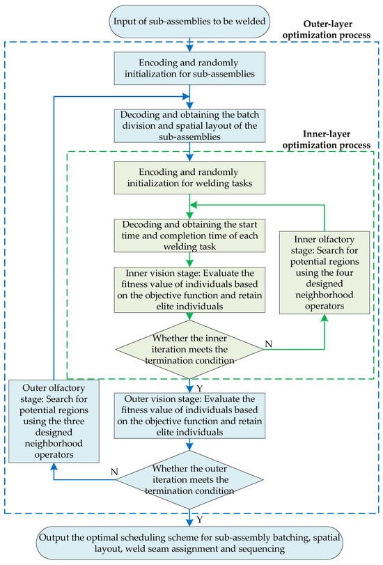
Figure 5. Flowchart of the improved two-layer fruit fly optimization algorithm.

After the completion of the inner-layer iteration, when the inner-layer optimization meets its convergence condition. The inner-layer outputs the finish time of the corresponding batch. This convergent feedback is then transmitted to the outer layer as the core evaluation basis for the current outer-layer solution. Next, the outer-layer vision phase evaluates the fitness of each individual in the sub-assembly-encoded population. The fitness value is comprehensively computed with reference to the finish time of all batches, which is aggregated from the convergent feedback of each batch’s inner-layer optimization. Based on this fitness evaluation, the roulette wheel selection method is also used to retain elite individuals with superior performance, ensuring the quality of the population for subsequent iterations. Similarly, in the olfaction phase of the outer-layer optimization process, three designed neighborhood operators are applied to search for more potential individuals in the solution space of sub-assembly encoding until the outer-layer iteration termination condition is satisfied. Finally, the optimal scheduling scheme, including sub-assembly batching, spatial layout, welding task assignment, and sequencing, are outputs.

4.1. Spatial Layout Method Under FOA (Outer-Layer Optimization Process)

4.1.1. Encoding and Initialization

A real-number encoding method is adopted for sub-assemblies, where each individual is represented by a chromosome. The length of the chromosome is equal to the number of sub-assemblies to be scheduled, denoted as J. Each gene in the chromosome is a real number between 0 and 1. The smallest gene value corresponds to the sub-assembly 1 with the smallest index. The second smallest gene value corresponds to the sub-assembly 2, and so on. Based on this encoding rule, an initial population containing $P_1$ chromosomes is randomly generated to form the initial population.

4.1.2. Decoding

The decoding process converts each chromosome in the population into a sub-assembly batching plan and a spatial layout plan.

Step 1. Convert the real-number-encoded chromosome into the corresponding sub-assembly sequence based on the encoding rule.

Step 2. Initialize an empty batch k and the corresponding available welding area.

Step 3. Attempt to place the first sub-assembly j in the sequence into the current batch k.

Step 4. If sub-assembly j can be placed in the current batch k, go to Step 5; otherwise, return to Step 2.

Step 5. Place sub-assembly j into batch k based on the heuristic rules for spatial layout (SLHR), update the usage status of the batch’s area, and remove sub-assembly j from the sub-assembly sequence.

Step 6. If all sub-assemblies have been scheduled, go to Step 7; otherwise, return to Step 3.

Step 7. End and output the sub-assembly batching scheme and the spatial layout scheme.

The heuristic rules for spatial layout (SLHR) are as follows:

Rule 1: Maximum load balancing rule

Due to the varying shapes and sizes of sub-assemblies in each batch, different welding task durations, and the limited working area of each robot, some robots may remain idle for extended periods. Therefore, the maximum load balancing rule is proposed: if sub-assembly j can be placed in batch k, select the placement posture $(X_j^P,Y_j^P,{\theta }_j^P)$ such that the variance of the total welding tasks in the feasible working area $(X_r^{CS},X_r^{CE})$, $(Y_r^{CS},Y_r^{CE})$ of each robot after placement is minimized. This rule directly addresses the load imbalance issue among robots, reducing unnecessary idle time and improving overall production efficiency of the welding line.

Rule 2: Large-area sub-assembly first rule

Due to the different shapes and sizes of sub-assemblies in each batch, large-area sub-assemblies may fail to be placed if scheduled later, leading to low space utilization. Therefore, the large-area sub-assembly first rule is proposed: after creating a new empty batch k, first determine the spatial positions $(X_j^P,Y_j^P)$ of large-area sub-assemblies (with base plate area above the overall third quartile) from the set of sub-assemblies to be scheduled. If these large-area sub-assemblies cannot be placed in batch k, then supplement with other sub-assemblies. This design ensures that key components with higher spatial requirements are reasonably arranged first, reducing the risk of batch splitting and improving scheduling continuity.

Rule 3: Long strip sub-assembly prioritizes the longitudinal placement rule

Since the interference between longitudinally placed sub-assemblies is relatively smaller than that between transversely placed ones, the longitudinal placement rule for long strip sub-assemblies is proposed. If the length $L_j$ of the sub-assembly is greater than 1.5 times its width $W_j$ and the length $L_j$ of the sub-assembly is less than the site width W, priority should be given to angle ${\theta }_j^P={90}^{\circ }$ or ${270}^{\circ }$. Longitudinal placement reduces the overlapping probability of welding ranges between adjacent sub-assemblies, effectively mitigating robot collision risks during operation.

Rule 4: The upper and lower robots sub-assembly with the most welding tasks, prioritize using the upper and lower robots

During sub-assembly placement, some sub-assemblies have multiple welding tasks and require a long operation time. The following rule is proposed to avoid mutual interference between robots on different sides during operation. If sub-assembly j can be placed in batch k, select the placement posture $(X_j^P,Y_j^P,{\theta }_j^P)$ such that the difference in the number of welding tasks of sub-assembly j between the upper half and the lower half is minimized. Balancing the number of welding tasks between the upper and lower halves enables the parallel operation of upper and lower robots, shortening the processing cycle of high-load sub-assemblies and reducing cross-side robot interference for complex tasks.

Rule 5: Minimum interference welding task first rule

Considering the limited spatial area, sub-assemblies with fewer interferences between their welding tasks should be placed together as much as possible. Therefore, the minimum interference welding task first rule is proposed. If sub-assembly j can be placed in batch k, select the placement posture $(X_j^P,Y_j^P,{\theta }_j^P)$ such that the total interference length between the welding tasks of sub-assembly j and those of other sub-assemblies already placed in batch k is minimized. Minimizing welding task interference to the greatest extent possible, reducing the need for robot waiting and path adjustment, and minimizing the probability of interference during the welding process.

4.1.3. Neighborhood Operator Design

In this study, three types of neighborhood operators are designed for sub-assembly encoding to search for better population individuals.

Operator 1: Randomly select one gene from the current chromosome and randomly insert it into another position in the chromosome.

Operator 2: Randomly select two genes from the current chromosome and swap their positions in the chromosome.

Operator 3: Randomly select two genes from the current chromosome and insert these two genes into other positions in the chromosome.

These operators complement each other to form a flexible local search framework. The single-gene insertion and two-gene swapping operators enhance the algorithm’s exploitation capability by fine-tuning local solution structures, while the two-gene insertion operator strengthens exploration by adjusting the relative sequence of key sub-assemblies without disrupting their internal correlation. Based on the above three neighborhood operators, in the outer olfactory phase, $N_1$ neighborhood solutions are generated for each individual in the population to facilitate the search for better sub-assembly batching and spatial layout schemes within the solution space.

In addition, to expand the exploration space of solutions, two population optimization mechanisms are designed.

(1) Disturbance mechanism: Based on the current solution, randomly apply a certain neighborhood structure to generate a new solution, providing a new starting point for subsequent local searches. It enhances the global exploration capability of the algorithm, enabling it to search a wider solution space for potential optimal schemes.

(2) Population diversity restoration mechanism: When it is detected that the normalized standard deviation of the population’s fitness values, denoted as $\sigma$, is less than the threshold, a certain proportion of the solutions in the population, denoted as $rr$, are randomly replaced with newly generated random solutions. Here, the replacement rate is 20%. The optimal values of $\sigma$ and $rr$ are determined through experiments, as detailed in Section 5.1. This design ensures that the algorithm maintains strong search vitality throughout the iteration process, improving the probability of finding the global optimal solution.

4.2. Sequence Optimization Method Under FOA (Inner-Layer Optimization Process)

4.2.1. Encoding and Initialization

Welding tasks are encoded using an integer encoding method. Each individual is represented by R segments of chromosomes, where each segment corresponds to a set of cantilever welding robots r, and the integers in each chromosome correspond to the indices i of the welding tasks in the batch.

During the individual initialization process, since welding tasks in the independent operation area $(X_r^{OS},X_r^{OE})$,$(Y_r^{OS},Y_r^{OE})$ can only be completed by the corresponding welding robot r, if part of a welding task is in this area, the entire welding task can only be welded by robot r, so the index i of this welding task can only be assigned to the chromosome corresponding to robot r. Subsequently, for welding tasks in the public area, they are randomly assigned to the chromosomes corresponding to the welding robots capable of performing those tasks. By repeating the above process, an initial population containing $P_2$ chromosomes is generated.

4.2.2. Decoding

The decoding process of the welding task sequence adopts a serial schedule generation mechanism.

Step 1: Set the scheduling time $t=0$ and initialize the index list of scheduled welding tasks as empty.

Step 2: Identify the welding robots that are idle at the current time.

Step 3: Find the next welding task to be welded from the chromosome of each idle welding robot to form a set of candidate welding tasks.

Step 4: If there is spatial interference between the welding tasks in the candidate set and those currently being performed, go to Step 5; otherwise, go to Step 6.

Step 5: Remove those welding tasks from the candidate set.

Step 6: If there is spatial interference between the allocatable regions of the tasks in the candidate set, go to Step 7; otherwise, go to Step 8.

Step 7: Compare the lengths of the pending welding tasks of the robots corresponding to the interfering welding tasks. The welding task of the robot with the longer pending welding task length is further removed from the candidate set.

Step 8: Place all remaining welding tasks in the candidate set, calculate their welding end times based on the welding time calculation rules, and remove the indices of these tasks from the corresponding robot chromosomes.

Step 9: Once all welding tasks are scheduled, move to Step 11; otherwise, go to Step 10.

Step 10: Choose the minimum completion time of the scheduled welding tasks exceeding the current scheduling time to serve as the next scheduling time, and return to Step 2.

Step 11: End and output the welding task assignment and welding schedule.

Through the above decoding method, a specific welding task encoding individual can be converted into the corresponding welding task assignment and welding schedule, and then the total idle duration of the batch is computed to evaluate the fitness value of the individual.

4.2.3. Neighborhood Operator Design

In this study, four types of neighborhood operators are designed for welding task encoding to search for better population individuals.

Operator 1: Randomly select one chromosome segment from the individual, then randomly select one gene from this chromosome and insert it into a random position within the same chromosome.

Operator 2: Randomly select one chromosome segment from the individual, then randomly select two genes from this chromosome and swap their positions.

Operator 3: Randomly select one chromosome segment from the individual, then randomly select one gene from this chromosome. If there are robots capable of performing the corresponding welding task, insert this gene into a random position in the chromosome corresponding to that robot.

Operator 4: Randomly select two genes from the individual. If the corresponding welding robots can both perform at least two welding tasks, randomly select two tasks from the public welding task set and insert them into random positions in the two chromosomes.

These operators create a targeted search framework for inner-layer optimization by combining local fine-tuning via gene insertions and swaps with cross-robot adjustments, using robot-based gene insertion and task exchanges. This balance of exploiting local solutions and exploring new task combinations prevents premature stagnation, ensuring effective welding task assignment and full use of robot capabilities. Based on the above four neighborhood operators, in the inner olfactory phase, $N_2$ neighborhood solutions are generated for each individual in the population to facilitate the search for better scheduling schemes for welding task assignment and sequencing in the solution space. The disturbance mechanism and population diversity restoration mechanism are also used in the iteration process to expand the exploration space of solutions.

4.3. Analysis of Algorithm Calculation Complexity

The computational cost of the improved two-layer fruit fly optimization algorithm (ITLFOA) stems primarily from the decoding and neighborhood search operations embedded in its two-layer nested structure. In outer-layer optimization, decoding each individual involves generating the spatial layout of sub-assemblies, with a time complexity of approximately $O\left(J\right)$, which is dominated by interference checking in heuristic layout rules. For inner-layer optimization, the decoding of welding task sequences adopts a serial schedule generation scheme, yielding a complexity of around $O\left(n\right)$, where n represents the total number of welding tasks per batch. The associated cost arises mainly from spatial interference checks for weld seam execution at each scheduling step. Thus, the total time complexity of the algorithm can be approximated as $O(G_1·P_1(J+G_2{P}_2{B}_n))$, where $G_1$, $G_2$ and $P_1$, $P_2$ refer to the iteration counts and population sizes for the outer and inner layers, respectively, and B denotes the number of batches.

Although this complexity exhibits polynomial growth, the number of sub-assemblies processed daily in practical automated sub-assembly welding line scheduling problems (ASWLSPs) rarely exceeds 100, and the task count n per batch is constrained by the physical dimensions of the welding area, ensuring that key problem parameters do not increase indefinitely. The parameter tuning presented in Section 5.1 of this paper is specifically designed to obtain high-quality solutions for problems of a given scale within an acceptable computational time frame ranging from several minutes to tens of minutes. In summary, the computational complexity of ITLFOA is manageable and practical for solving real-world scheduling problems in shipyards, demonstrating favorable engineering scalability. Finally, the pseudocode of ITLFOA is shown in Algorithm 1.

Algorithm 1 ITLFOA Algorithm

Require:  An automated sub-assembly welding line scheduling problem (ASWLSP), outer-layer maximum iteration count $G_{1,max}$, inner-layer maximum iteration count $G_{2,max}$ Ensure:  Optimal scheduling scheme  1: Generate outer-layer initial population $P_{\mathrm{outer}}$, set $G_1=0$  2: while $G_1<G_{1,max}$ do  3:     for all individual $p_{i,\mathrm{outer}}\in P_{\mathrm{outer}}$ do  4:         Decode $p_{i,\mathrm{outer}}$: sub-assembly batching and spatial layout  5:         Obtain batch set $B=\{B_1,B_2,\dots ,B_k\}$  6:         for all batch $B_k\in B$ do  7:            Generate inner-layer initial population $P_{\mathrm{inner}}$, set $G_2=0$  8:            while $G_2<G_{2,max}$ do  9:                for all individual $p_{j,\mathrm{inner}}\in P_{\mathrm{inner}}$ do 10:                    Decode $p_{j,\mathrm{inner}}$: seam assignment and sequencing 11:                    Evaluate fitness (batch completion time $M_k$) 12:                end for 13:                Select elite individuals via roulette wheel selection 14:                Update $P_{\mathrm{inner}}$ using 4 neighborhood operators with disturbance mechanism 15:                $G_2=G_2+1$ 16:            end while 17:            Get optimal batch completion time $M_k^{*}$ 18:         end for 19:         Compute total makespan: ${\mathrm{Total}}_M={\sum }_{k=1}^K{M}_k^{*}$ 20:         Select elite individuals in $P_{\mathrm{outer}}$ via roulette wheel selection 21:         Update $P_{\mathrm{outer}}$ using 3 neighborhood operators with disturbance mechanism 22:         Update $P_{\mathrm{outer}}$ with diversity restoration mechanism 23:         $G_1=G_1+1$ 24:     end for 25: end while 26: Output the optimal scheduling scheme

5. Results and Discussions

This paper uses partial data from a shipyard to form a solution case. The baseline case includes 30 sub-assemblies $(J=30)$, the space size is $(11,7)\left(\right(L,W)=(11,7\left)\right)$. The safety distance between welding robots on the same side is 3.5 $(SD=3.5\mathrm{m})$, the safety distance between welding robots on opposite sides is 3 $(DD=3\mathrm{m})$, and the additional working distance in the Y-direction for welding robots at the junction of the upper and lower rollers is 0.2 $(MD=0.2\mathrm{m})$.

The effective working areas and independent working areas of each welding robot are detailed in Table 3. All units related to spatial dimensions are meters.

Table 3. Feasible and independent working areas of welding robots (unit: meters).

Welding Robots	Feasible Working Area	Independent Working Area
robot 1	$(X_1^{CS},X_1^{CE}),(Y_1^{CS},Y_1^{CE})$$=(0,7.5),(0,3.7)$	$(X_1^{CS},X_{1}6CE),(Y_{1}6CS,Y_1^{CE})$$=(0,3.5),(0,3.5)$
robot 2	$(X_2^{CS},X_2^{CE}),(Y_2^{CS},Y_2^{CE})$$=(3.5,11),(0,3.7)$	$(X_2^{CS},X_2^{CE}),(Y_{2}6CS,Y_2^{CE})$$=(7.5,11),(0,3.5)$
robot 3	$(X_3^{CS},X_3^{CE}),(Y_3^{CS},Y_3^{CE})$$=(0,7.5),(3.3,7)$	$(X_3^{CS},X_3^{CE}),(Y_3^{CS},Y_3^{CE})$$=(0,3.5),(3.5,7)$
robot 4	$(X_4^{CS},X_4^{CE}),(Y_4^{CS},Y_4^{CE})$$=(3.5,11),(3.3,7)$	$(X_4^{CS},X_4^{CE}),(Y_4^{CS},Y_4^{CE})$$=(7.5,11),(3.5,7)$

5.1. Parameter Settings

The key parameters to be determined for the proposed ITLFOA include outer-layer population size $P_1$, inner-layer population size $P_2$, the number of neighborhood solutions generated in the outer layer $N_1$, and the number of neighborhood solutions generated in the inner-layer $N_2$. Taguchi design approach is adopted to identify the optimal settings of these parameters. The value ranges of these parameters are $P_1\in \{20,30,40\}$, $P_2\in \{20,30,40\}$, $N_1\in \{1,2,3\}$, $N_2\in \{1,2,3\}$, as shown in Table 4; $L_2(3^4$) orthogonal experimental combinations are selected. The algorithm is executed ten times per experimental combination, and the obtained objective function values are used as response values.

Table 4. Reference Values for Parameter Testing.

Parameters	Level Value
	1	2	3
$P_1$	20	30	40
$P_2$	20	30	40
$N_1$	1	2	3
$N_2$	1	2	3

Eventually, the main effect plots of the mean value and signal-to-noise ratio are shown in Figure 6 and Figure 7. Analysis of these figures reveals that the minimum mean response and maximum signal-to-noise ratio are achieved when parameters $P_1$, $P_2$, $N_1$, and $N_2$ are set to levels 2, 3, 1, and 1, respectively. Consequently, the optimal parameter combination was selected as $P_1=30$, $P_2=40$, $N_1=1$, $N_2=1$. Furthermore, the relative importance of these parameters, in descending order, was determined from Table 5 as $N_2$, $N_1$, $P_1$, $P_2$.

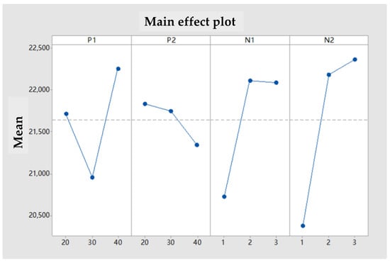
Figure 6. Main effect plot of means.

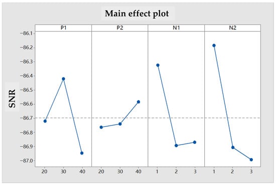
Figure 7. Main effect plot of Signal-to-Noise Ratio (SNR).

Table 5. Mean Response Table.

Level	${\mathit{P}}_1$	${\mathit{P}}_2$	${\mathit{N}}_1$	${\mathit{N}}_2$
1	21,715	21,831	20,730	20,381
2	20,953	21,745	22,108	22,181
3	22,255	21,348	22,085	22,362
Delta	1302	483	1378	1981
Ranking	3	4	2	1

To further justify the chosen values for the population diversity restoration mechanism’s normalized standard deviation threshold ($\sigma$) and the solution replacement rate ($rr$), an additional experimental study was conducted. With the optimal settings of $P_1=30$, $P_2=40$, $N_1=1$, $N_2=1$ fixed, we systematically evaluated various combinations of $\sigma \in \{0.2,0.3,0.4\}$ and $rr\in \{10\%,20\%,30\%\}$. Each combination was executed three times independently, and the average makespan was recorded. The results, presented in Table 6, demonstrate that the combination of $\sigma =0.3$ and $rr=20\%$ yields the most favorable performance, achieving the lowest average makespan. This experimental validation supports our selection of these critical parameters for the population diversity restoration mechanism.

Table 6. Experimental Evaluation of Population Diversity Restoration Mechanism Parameters.

$\mathit{\sigma }$	$\mathit{rr}$			Mean
	10%	20%	30%
0.2	19,588.0	18,879.7	20,072.3	19,513.3
0.3	19,050.3	18,857.0	19,430.3	19,112.5
0.4	20,697.0	20,399.7	19,965.0	20,353.9
mean	19,778.4	19,378.8	19,822.5	19,659.9

5.2. Performance Verification of the Proposed Algorithm

The performance of the proposed ITLFOA is comprehensively evaluated from three aspects to verify its efficiency and superiority. First, the solutions obtained by ITLFOA are compared with the current manual scheduling scheme. Second, the initial version of TLFOA (without the proposed improvements) is applied to the same problem for a direct performance comparison. Third, the Variable Neighborhood Search (VNS) algorithm, is introduced as an additional benchmark to contextualize the performance within broader optimization methodologies. These algorithms all use the same termination criteria, specifically the outer-layer maximum iteration count $G_{1,max}$ is 60, and the inner-layer maximum iteration count $G_{2,max}$ is 80.

5.2.1. Comparative Analysis with Manual Scheduling Results

In actual production, the approach adopted by engineers to obtain the spatial layout of sub-assemblies is as follows. At first, the large-area sub-assemblies are placed at the bottom-left or bottom-right corner; then, the small-area sub-assemblies in accordance with the principle of enhancing space utilization are placed in the vacant areas of the work space based on the principle of improving space utilization, but the choice of specific placement positions is relatively arbitrary.

Next, to allocate the weld seams, the welds within the feasible welding area are evenly partitioned between the two sets of welding systems based on the quantity of welds in their respective independent working areas.

In determining the welding sequence, the same-side welding robot adopts the sequence of vertical welding first, then flat welding, followed by welding along the main welding direction X. If there are welding tasks in the secondary welding direction Y within a certain X interval, the system switches to the welding tasks in the Y-direction. After completing the welding tasks in the secondary welding direction Y, it continues welding along the main welding direction, as shown in Figure 8.

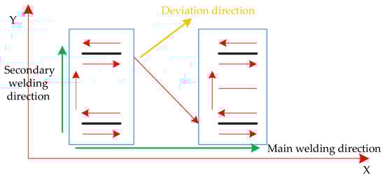
Figure 8. Schematic diagram of welding direction.

In the independent welding area, the two welding robots adopt collision avoidance strategies to prevent collisions, i.e., following collision avoidance strategy and opposing collision avoidance strategy, as shown in Figure 9 and Figure 10.

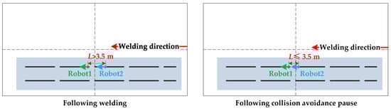
Figure 9. Following collision avoidance principle.

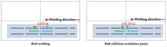
Figure 10. Opposing collision avoidance principle.

(1) Following collision avoidance strategy: When welding in the same direction, if the distance between the two robots is greater than $3.5$ m, they can perform following welding; otherwise, the robots will pause for safety reasons and wait for manual handling.

(2) Opposing collision avoidance strategy: When welding in opposite directions, if the distance between the two robots is greater than $3.5$ m, they can perform opposing welding; otherwise, the robots will pause for safety reasons and wait for manual handling.

Eventually, the manual scheduling results are shown in Figure 11, Figure 12, Figure 13, Figure 14, Figure 15, Figure 16, Figure 17, Figure 18, Figure 19 and Figure 20. To aid in the interpretation of the scheduling results (Figure 11, Figure 12, Figure 13, Figure 14, Figure 15, Figure 16, Figure 17, Figure 18, Figure 19 and Figure 20), the graphical elements are explained as follows: Each block represents a welding task. The black number inside a block denotes the unique identifier of the welding seam within its current batch. The blue annotation associated with each block provides detailed information about the corresponding sub-assembly, formatted as $\left[Index\right]:\left[Type\right],(X,Y,\theta )$. For example, the annotation 0: 108B, (0, 5.3, 0) indicates that this task belongs to sub-assembly #0, of type 108B, positioned at coordinates (0, 5.3) with a rotation angle ($\theta$) of 0 degrees.

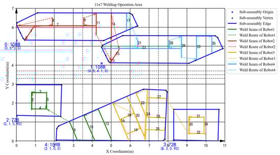
Figure 11. Spatial layout of batch 1 in the manual scheduling results.

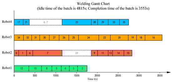
Figure 12. Gantt chart for sequence optimization of batch 1 in the manual scheduling results.

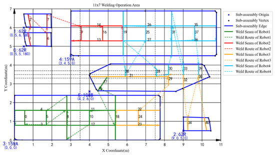
Figure 13. Spatial layout of batch 2 in the manual scheduling results.

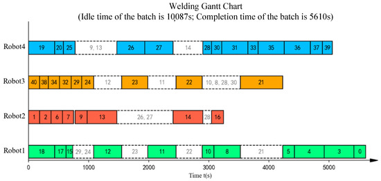
Figure 14. Gantt chart for sequence optimization of batch 2 in the manual scheduling results.

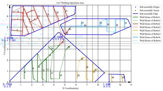
Figure 15. Spatial layout of batch 3 in the manual scheduling results.

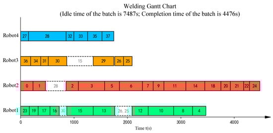
Figure 16. Gantt chart for sequence optimization of batch 3 in the manual scheduling results.

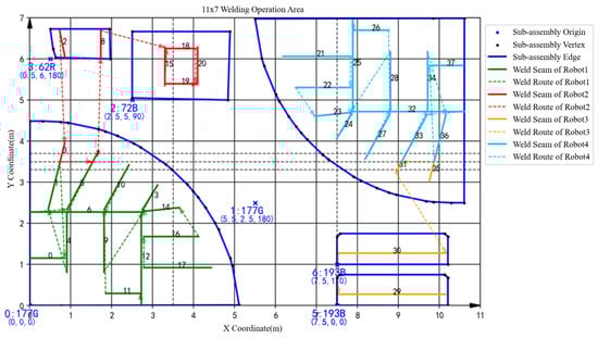
Figure 17. Spatial layout of batch 4 in the manual scheduling results.

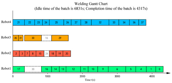
Figure 18. Gantt chart for sequence optimization of batch 4 in the manual scheduling results.

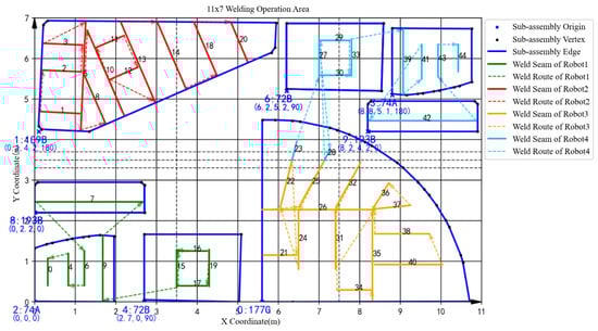
Figure 19. Spatial layout of batch 5 in the manual scheduling results.

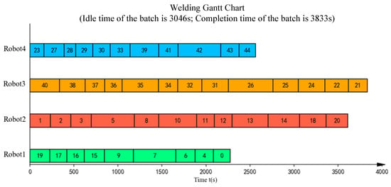
Figure 20. Gantt chart for sequence optimization of batch 5 in the manual scheduling results.

The scheduling results obtained by a single run of the proposed ITLFOA for the same case are shown in Figure 21, Figure 22, Figure 23, Figure 24, Figure 25, Figure 26, Figure 27, Figure 28, Figure 29 and Figure 30. The comparison of the results obtained by ITLFOA and manual operation is shown in Table 7.

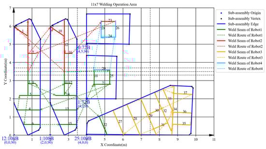
Figure 21. Spatial layout of batch 1 in the manual scheduling results.

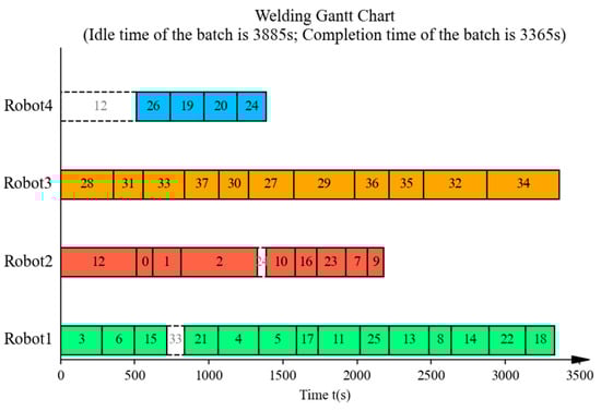
Figure 22. Gantt chart for sequence optimization of batch 1 in the manual scheduling results.

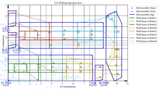
Figure 23. Spatial layout of batch 2 in the manual scheduling results.

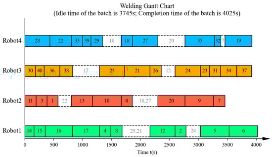
Figure 24. Gantt chart for sequence optimization of batch 2 in the manual scheduling results.

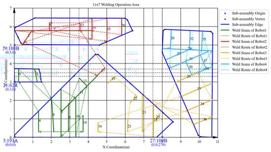
Figure 25. Spatial layout of batch 3 in the manual scheduling results.

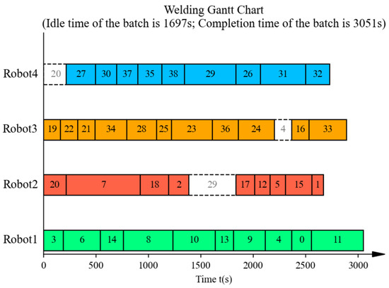
Figure 26. Gantt chart for sequence optimization of batch 3 in the manual scheduling results.

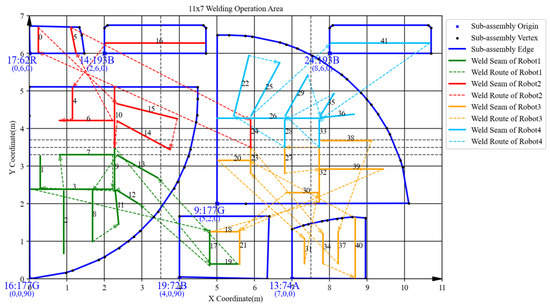
Figure 27. Spatial layout of batch 4 in the manual scheduling results.

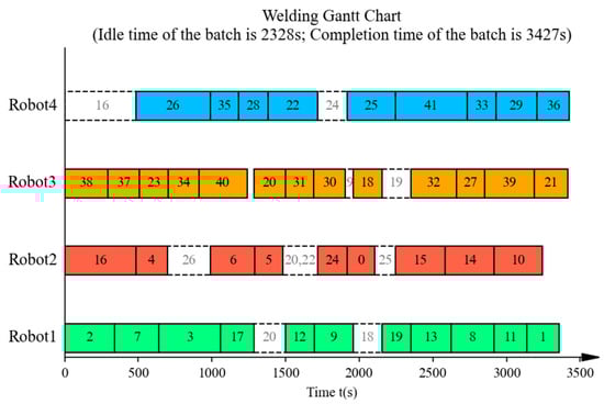
Figure 28. Gantt chart for sequence optimization of batch 4 in the manual scheduling results.

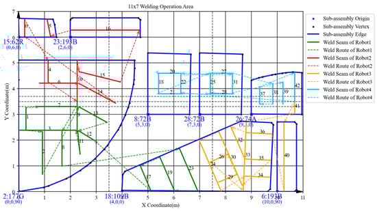
Figure 29. Spatial layout of batch 5 in the manual scheduling results.

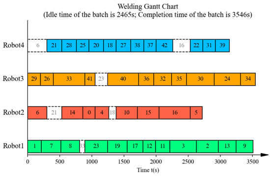
Figure 30. Gantt chart for sequence optimization of batch 5 in the manual scheduling results.

Table 7. The comparison of the results obtained by ITLFOA and manual operation.

Batch	Manual Operation		ITLFOA
	Idle Time (s)	Completion Time (s)	Idle Time (s)	Completion Time (s)
batch 1	4815	3553	3885	3365
batch 2	10,087	5610	3745	4025
batch 3	7487	4476	1697	3051
batch 4	6831	4317	2328	3427
batch 5	3046	3833	2465	3546
Total	32,266	21,789	14,120	17,414

As shown in Figure 11, Figure 12, Figure 13, Figure 14, Figure 15, Figure 16, Figure 17, Figure 18, Figure 19, Figure 20, Figure 21, Figure 22, Figure 23, Figure 24, Figure 25, Figure 26, Figure 27, Figure 28, Figure 29 and Figure 30 and Table 7, the proposed ITLFOA has distinct advantages in solving ASWLSP compared with manual scheduling. Regarding the total idle time, the result derived from ITLFOA is 14,120 s, while the result in manual operation is 32,266 s, compared with manual operation, the proposed ITLFOA reduces by 18,146 s, which means an improvement of 56.24%. Meanwhile, in terms of the total completion time, the result obtained by ITLFOA is 17,414 s, while the result in manual operation is 21,789 s, compared with manual operation, the proposed ITLFOA reduces by 4375 s, which means an improvement of 20.08%.

Further analysis of the scheduling results of each batch reveals obvious load imbalance in batches 3, 4, and 5 in the manual operation. Because during the process of determining the spatial layout of sub-assemblies, manual scheduling mainly focus on space utilization without considering load balancing. In addition, there is frequent equipment interference waiting in batch 2. This is due to the fact that robots on the same side are more prone to welding interference in the complex welding task distribution areas under the strategy “same side identical, opposite sides reversed”. In detail, a comparison of the sub-assembly spatial layouts reveals that the key difference stems from sub-assembly 108B. In the spatial layout of batch 2 obtained by ITLFOA (Figure 23), sub-assembly 108B is placed longitudinally, enabling the uniform distribution of its welding load between the upper and lower halves of the welding area. Consequently, the workloads of the upper and lower robots are more balanced, leading to nearly identical processing times among the four robots during subsequent weld scheduling. In contrast, in spatial layout of batch 2 of the manual scheduling results (Figure 13), sub-assembly 108B is placed transversely, resulting in most welding tasks being assigned to the lower half. This causes robots 1 and 3 to bear longer welding tasks, leading to unbalanced robot loads during weld scheduling. Meanwhile, the transverse placement of the longest welding task (task 21) results in processing interference with multiple other welding tasks. As illustrated in Figure 14, welding task 21 forces both robots 3 and 1 to experience prolonged waiting times, further extending the completion time of robot 1. Collectively, these two factors result in the longer completion time of batch 2 in the manual scheduling results. It fully demonstrates the effectiveness of the heuristic rules for spatial layout proposed in the ITLFOA.

5.2.2. Performance Comparison of ITLFOA, Initial TLFOA, and VNS

To the best of our knowledge, few published studies have specifically addressed the scheduling problem of automated sub-assembly welding lines, especially those integrating spatial layout and robot interference constraints. To provide a comprehensive evaluation of ITLFOA’s performance, we compare it against both its foundational version (initial TLFOA) and a well-established metaheuristic algorithm, Variable Neighborhood Search (VNS). It mainly aims to verify the effectiveness of several key improved designs proposed in the algorithm of this paper: the heuristic rules for spatial layout; the improved neighborhood operators; the added disturbance mechanism and population diversity restoration mechanism. The difference between of the ITLFOA and initial TLFOA is shown in Table 8. The comparison of the results obtained by ITLFOA, initial TLFOA and VNS is shown in Table 9. For VNS, standard parameter settings were employed.

Table 8. The difference between the ITLFOA and initial TLFOA.

Difference	Initial TLFOA	ITLFOA
space layout rule	maximum remaining rectangle	SLHR
neighborhood operator 3 in the outer-layer	adjacent position swapping	random insertion strategy
disturbance mechanism	none	random disturbance with neighborhood structures
population diversity	none	adaptive population refresh strategy

Table 9. The comparison of the results obtained by ITLFOA, initial TLFOA, and VNS.

Batch	ITLFOA		Initial TLFOA		VNS
	Idle Time	Completion Time	Idle Time	Completion Time	Idle Time	Completion Time
batch 1	3885 s	3365 s	2722 s	3365 s	3067 s	4363 s
batch 2	3745 s	4025 s	4890 s	4125 s	6698 s	3866 s
batch 3	1697 s	3051 s	6162 s	4021 s	1394 s	3002 s
batch 4	2328 s	3427 s	3594 s	3833 s	4319 s	4088 s
batch 5	2465 s	3546 s	2399 s	3392 s	2636 s	3026 s
Total	14,120 s	17,414 s	19,767 s	18,736 s	18,114 s	18,345 s

It can be seen from Table 9 that compared with the initial TLFOA and VNS, the ITLFOA proposed in this paper still exhibits favorable performance in both the total idle time and the total completion time. This demonstrates the effectiveness of the improved designs in ITLFOA, such as the heuristic rules for spatial layout, the improved neighborhood operators, the added disturbance mechanism, and the added population diversity restoration mechanism. In addition, compared with the initial manual operation results, the scheduling results obtained by the initial TLFOA have also a notable enhancement, which indirectly confirms the effectiveness of the two-layer algorithm structure of TLFOA.

To sum up, the comparison results of the above two aspects can prove that for ASWLSP, the proposed ITLFOA achieves better performance in terms of the design of the two-layer algorithm structure and the improvement of the improved designs.

5.2.3. Robustness and Statistical Analysis Across Problem Scales

To assess the robustness and statistical reliability of the proposed algorithm, experiments were extended to problem instances of different scales, specifically with 20, 30, 40, 50, 60, 70, and 80 sub-assemblies $(J20,J30,J40,J50,J60,J70,J80)$. For each case and each algorithm (Initial TLFOA, VNS, ITLFOA), three independent runs were executed. The mean and standard deviation of the total completion time are reported in Table 10. This approach allows for an evaluation of performance consistency and sensitivity to problem size.

Table 10. Statistical comparison of makespan (mean ± standard deviation) across different problem scales and algorithm.

Case	ITLFOA	Initial TLFOA	VNS
$J20$	10,673.3 ± 269.3	10,953.3 ± 41.3	11,457.7 ± 158.3
$J30$	18,108.0 ± 654.8	18,894.7 ± 577.6	19,994.7 ± 1447.0
$J40$	27,328.7 ± 959.0	28,620.3 ± 492.7	30,221.7 ± 1151.2
$J50$	35,067.0 ± 880.6	36,547.3 ± 421.5	38,589.3 ± 321.0
$J60$	39,687.3 ± 587.3	40,938.7 ± 180.7	43,054.0 ± 33.2
$J70$	48,425.3 ± 773.3	49,252.0 ± 676.4	50,096.3 ± 596.3
$J80$	61,571.0 ± 1757.8	63,370.3 ± 1797.6	66,797.0 ± 421.0

As evidenced by Table 10, the proposed ITLFOA consistently outperforms both the initial TLFOA and VNS across all tested problem scales.

6. Conclusions

Amid the global wave of intelligent manufacturing and Industry 4.0, China’s shipbuilding industry boasting a 16-year consecutive global market share leadership faces acute contradictions between surging market demand and labor-intensive, inefficient production modes. Harsh working environments and a worsening “labor shortage” have further highlighted the urgency of automated transformation. As the smallest and most numerous composite units of ship hulls, sub-assemblies have become the primary breakthrough for shipyards to realize automation. The scheduling of automated sub-assembly welding lines, as a core link connecting component processing and block integration, not only determines the efficiency of shipbuilding production but also aligns with the national strategy of “digital shipbuilding” and the broader industrial trend of integrating batch processing, spatial layout, and multi-robot collaboration.

This study focuses on the automated sub-assembly welding line scheduling problem (ASWLSP) in shipyards, a complex constrained optimization problem involving multiple intertwined decision dimensions: sub-assembly batching, spatial lay-out planning, multi-robot task allocation, and welding sequence optimization. Unlike conventional scheduling problems, ASWLSP must address unique industry-specific constraints, including collision avoidance between same-side and opposite-side robots (with safety distances of 3.5 m and 3 m, respectively), limited robot working areas, and load balancing among eight robots grouped into four cantilever systems. The core challenge lies in resolving the nested dependency between global decisions (sub-assembly sequencing, batching, and spatial layout) and local decisions (welding task assignment and sequencing) to minimize the total completion time (makespan) while ensuring no spatial overlap of sub-assemblies, full coverage of welding tasks, and compliance with robot operational constraints.

To solve this problem, a mathematical model taking minimizing the makespan as its objective function is constructed, and an improved two-layer fruit fly optimization algorithm (ITLFOA) is proposed. In the outer-layer optimization process, the design of heuristic decoding algorithms, three neighborhood operators, a disturbance mechanism, and a population diversity restoration mechanism are proposed to optimize sub-assembly sequencing, sub-assembly batching, and sub-assembly spatial layout. In the inner-layer optimization process, heuristic decoding algorithms, four neighborhood operators, a disturbance mechanism, and a population diversity restoration mechanism are designed to obtain welding task assignment and welding task sequencing. Afterwards, the solutions of the outer-layer optimization will be further adjusted according to the results of the inner-layer optimization. Through such interaction between the inner and outer layers, the scheduling scheme for the automated sub-assembly welding line is obtained. Finally, the performance verification is carried out on a specific case of a shipyard. By comparing with the initial two-layer fruit fly optimization algorithm and the results obtained by the shipyard based on actual manual experience, the validity of ITLFOA is illustrated.

The scheduling problem of automated sub-assembly welding lines is a practically important engineering challenge for shipyards, and it enriches the existing research on resource-constrained scheduling by incorporating unique industry characteristics. It demonstrates cross-scenario adaptability, particularly in industrial settings that utilize gantry and cantilever robots for batch processing. These scenarios demand the coordinated integration of workpiece arrangement, task allocation, and multi-robot operation under specific operational constraints. Although the proposed ITLFOA has achieved relatively optimal solutions, the two-layer nested structure increases the algorithm’s computational complexity, which may affect its real-time performance in large-scale scheduling scenarios. In further research, a hybrid algorithm combining ITLFOA with deep learning mechanisms can be taken into consideration to improve the adaptability and solving speed of the algorithm through automatically extracting spatial layout features and welding task correlation patterns from historical data. In addition, only a single shipyard case has been considered. More diverse cases of different production line configurations, even in other manufacturing industries, can be used to test the performance of the proposed algorithm.

Generally, this study fills a research gap in ASWLSP by establishing the first coupled optimization model and a tailored ITLFOA, systematically addressing the nested decision-making challenges of automated sub-assembly welding line scheduling. It not only provides a practical solution for shipyards to achieve efficient, intelligent scheduling but also enriches the theoretical framework of resource-constrained scheduling by integrating industry-specific constraints (e.g., robot collision avoidance, spatial layout heuristics). The findings and methodologies presented offer valuable insights for promoting the transformation of labor-intensive manufacturing industries toward automation and intelligence, contributing to the advancement of global smart manufacturing practices.

References

- CANSI. China’s Shipbuilding Industry Maintains Global Lead in Three Major Indicators for the First Three Quarters of 2025. Available online: https://www.cansi.org.cn/cms/document/19761.html (accessed on 17 October 2025).
- Liu, W.; Kuang, Z.; Zhang, Y.; Zhou, B.; He, P.; Li, S. An effective hybrid genetic algorithm for the multi-robot task allocation problem with limited span. Expert Syst. Appl. 2025, 280, 127299. [Google Scholar] [CrossRef]
- Shi, D.; Fan, W.; Xiao, Y.; Lin, T.; Xing, C. Intelligent scheduling of discrete automated production line via deep reinforcement learning. Int. J. Prod. Res. 2020, 58, 3362–3380. [Google Scholar] [CrossRef]
- Bai, L.; Wu, N.; Li, Z.; Zhou, M. Optimal one-wafer cyclic scheduling and buffer space configuration for single-arm multicluster tools with linear topology. IEEE Trans. Syst. Man Cybern. Syst. 2016, 46, 1456–1467. [Google Scholar] [CrossRef]
- Yang, F.; Wu, N.; Qiao, Y.; Su, R. Polynomial approach to optimal one-wafer cyclic scheduling of treelike hybrid multi-cluster tools via Petri nets. IEEE/CAA J. Autom. Sin. 2017, 5, 270–280. [Google Scholar] [CrossRef]
- Manzini, M.; Demeulemeester, E.; Urgo, M. A predictive–reactive approach for the sequencing of assembly operations in an automated assembly line. Robot. Comput.-Integr. Manuf. 2022, 73, 102201. [Google Scholar] [CrossRef]
- Sriskandarajah, C.; Drobouchevitch, I.; Sethi, S.P.; Chandrasekaran, R. Scheduling multiple parts in a robotic cell served by a dual-gripper robot. Oper. Res. 2004, 52, 65–82. [Google Scholar] [CrossRef]
- Kim, H.J.; Lee, J.H. Scheduling of dual-gripper robotic cells with reinforcement learning. IEEE Trans. Autom. Sci. Eng. 2021, 19, 1120–1136. [Google Scholar] [CrossRef]
- Kim, H.J.; Lee, J.H. Look-ahead based reinforcement learning for robotic flow shop scheduling. J. Manuf. Syst. 2023, 68, 160–175. [Google Scholar] [CrossRef]
- Lee, J.H.; Kim, H.J. Optimal Scheduling of Timed Petri Nets With Resource Marking and Ready Times: Application to Robotic Flow Shops. IEEE Robot. Autom. Lett. 2025, 10, 3684–3691. [Google Scholar] [CrossRef]
- Wang, J.; Zhou, H.; Guo, J.; Si, H.; Chen, X.; Zhang, M.; Zhang, Y.; Zhou, G. A Q-Learning-based Deep Deterministic Policy Gradient Algorithm for the Re-entrant Hybrid Flow Shop Joint Scheduling Problem with Dual-gripper. Eng. Lett. 2025, 33, 1632–1647. [Google Scholar]
- Mao, Z.; Wang, W.; Sun, Y.; Fang, K. Job shop scheduling problem with a dual-gripper robot. IISE Trans. 2025, 1–16. [Google Scholar] [CrossRef]
- Ghadiri Nejad, M.; Kovács, G.; Vizvári, B.; Barenji, R.V. An optimization model for cyclic scheduling problem in flexible robotic cells. Int. J. Adv. Manuf. Technol. 2018, 95, 3863–3873. [Google Scholar] [CrossRef]
- Liu, S.Q.; Kozan, E. A hybrid metaheuristic algorithm to optimise a real-world robotic cell. Comput. Oper. Res. 2017, 84, 188–194. [Google Scholar] [CrossRef]
- Gultekin, H.; Dalgıç, Ö.O.; Akturk, M.S. Pure cycles in two-machine dual-gripper robotic cells. Robot. Comput.-Integr. Manuf. 2017, 48, 121–131. [Google Scholar] [CrossRef][Green Version]
- Wang, D.; Liu, S.; Zou, J.; Qiao, W.; Jin, S. Flexible robotic cell scheduling with graph neural network based deep reinforcement learning. J. Manuf. Syst. 2025, 78, 81–93. [Google Scholar] [CrossRef]
- Hofmann, T.; Wenzel, D. How to minimize cycle times of robot manufacturing systems. Optim. Eng. 2021, 22, 895–912. [Google Scholar] [CrossRef]
- Helmberg, C.; Hofmann, T.; Wenzel, D. Periodic event scheduling for automated production systems. INFORMS J. Comput. 2022, 34, 1291–1304. [Google Scholar] [CrossRef]
- Wang, T.; Zhang, Y.; Hu, X. A Q-learning based hyper-heuristic scheduling algorithm with multi-rule selection for sub-assembly in shipbuilding. Comput. Ind. Eng. 2024, 197, 110567. [Google Scholar] [CrossRef]
- Lee, K.J.; Lee, J.K.; Choi, S.Y. A spatial scheduling system and its application to shipbuilding: DAS-CURVE. Expert Syst. Appl. 1996, 10, 311–324. [Google Scholar] [CrossRef]
- Lozano-Perez, T. Spatial planning: A configuration space approach. IEEE Trans. Comput. 1983, 32, 108–120. [Google Scholar] [CrossRef]
- Koh, S.; Eom, C.; Jang, J.; Choi, Y. An improved spatial scheduling algorithm for block assembly shop in shipbuilding company. In Proceedings of the 2008 3rd International Conference on Innovative Computing Information and Control; IEEE: Washington, DC, USA, 2008; p. 253. [Google Scholar]
- Shin, J.G.; Kwon, O.H.; Ryu, C. Heuristic and metaheuristic spatial planning of assembly blocks with process schedules in an assembly shop using differential evolution. Prod. Plan. Control 2008, 19, 605–615. [Google Scholar] [CrossRef]
- Shang, Z.; Gu, J.; Ding, W.; Duodu, E.A. Spatial scheduling optimization algorithm for block assembly in shipbuilding. Math. Probl. Eng. 2017, 2017, 1923646. [Google Scholar] [CrossRef]
- Ge, Y.; Wang, A. Spatial scheduling for irregularly shaped blocks in shipbuilding. Comput. Ind. Eng. 2021, 152, 106985. [Google Scholar] [CrossRef]
- Kwon, B.; Lee, G.M. Spatial scheduling for large assembly blocks in shipbuilding. Comput. Ind. Eng. 2015, 89, 203–212. [Google Scholar] [CrossRef]
- Dixit, V.; Verma, P.; Raj, P.; Sharma, M. Resource and time criticality based block spatial scheduling in a shipyard under uncertainty. Int. J. Prod. Res. 2018, 56, 6993–7007. [Google Scholar] [CrossRef]
- Ge, Y.; Wang, A. Spatial scheduling strategy for irregular curved blocks based on the modified genetic ant colony algorithm (MGACA) in shipbuilding. Int. J. Prod. Res. 2018, 56, 3099–3115. [Google Scholar] [CrossRef]
- Hu, S.; Liu, T.; Wang, S.; Kao, Y.; Sun, X. A hybrid heuristic algorithm for ship block construction space scheduling problem. Discret. Dyn. Nat. Soc. 2015, 2015, 841637. [Google Scholar] [CrossRef]
- Shen, Y.; Gao, Y.; Yuan, M.; Sun, H.; Guo, Z. Multi-objective immune optimization of path planning for ship welding robot. Electronics 2023, 12, 2040. [Google Scholar] [CrossRef]
- Meng, C.; Feng, Z.; Zhao, D.; Li, X.; Yu, J.; Yang, L. A Fuzzy Scheduling Method for Pipeline Processing in Shipyards Incorporating the Black Widow Optimization Algorithm. Appl. Sci. 2024, 14, 5639. [Google Scholar] [CrossRef]
- Han, Y.; Gong, D.; Li, J.; Zhang, Y. Solving the blocking flow shop scheduling problem with makespan using a modified fruit fly optimisation algorithm. Int. J. Prod. Res. 2016, 54, 6782–6797. [Google Scholar] [CrossRef]
- Wang, C.; Li, S. Hybrid fruit fly optimization algorithm for solving multi-compartment vehicle routing problem in intelligent logistics. Adv. Prod. Eng. Manag. 2018, 13, 466–478. [Google Scholar] [CrossRef]
- Shang, Z.; Chen, Y.; Mumtaz, J. An Improved Fruit Fly Optimization Algorithm for Multi-Objective Scheduling in Hybrid Flow Shops. Eng. Proc. 2025, 111, 37. [Google Scholar]
- Wang, L.; Zheng, X.l. A knowledge-guided multi-objective fruit fly optimization algorithm for the multi-skill resource constrained project scheduling problem. Swarm Evol. Comput. 2018, 38, 54–63. [Google Scholar] [CrossRef]
- Ma, Q.; He, Y.; Zhou, F. Multi-objective fruit fly optimization algorithm for test point selection. In 2016 IEEE Advanced Information Management, Communicates, Electronic and Automation Control Conference (IMCEC); IEEE: New York, NY, USA, 2016; pp. 272–276. [Google Scholar]
Disclaimer/Publisher’s Note: The statements, opinions and data contained in all publications are solely those of the individual author(s) and contributor(s) and not of MDPI and/or the editor(s). MDPI and/or the editor(s) disclaim responsibility for any injury to people or property resulting from any ideas, methods, instructions or products referred to in the content. |
© 2026 by the authors. Licensee MDPI, Basel, Switzerland. This article is an open access article distributed under the terms and conditions of the Creative Commons Attribution (CC BY) license.