


Abstract
With the advancement of Light Detection and Ranging (LiDAR) technology and computer science, LiDAR–Inertial Simultaneous Localization and Mapping (SLAM) has become essential in autonomous driving, robotic navigation, and 3D reconstruction. However, dynamic objects such as pedestrians and vehicles, with complex terrain conditions, pose serious challenges to existing SLAM systems. These factors introduce artifacts into the acquired point clouds and result in significant vertical drift in SLAM trajectories. To address these challenges, this study focuses on controlling vertical drift errors in LiDAR–Inertial SLAM systems operating in dynamic environments. The research focuses on three key aspects: ground point segmentation, dynamic artifact removal, and vertical drift optimization. In order to improve the robustness of ground point segmentation operations, this study proposes a method based on a concentric sector model. This method divides point clouds into concentric regions and fits flat surfaces within each region to accurately extract ground points. To mitigate the impact of dynamic objects on map quality, this study proposes a removal algorithm that combines multi-frame residual analysis with curvature-based filtering. Specifically, the algorithm tracks residual changes in non-ground points across consecutive frames to detect inconsistencies caused by motion, while curvature features are used to further distinguish moving objects from static structures. This combined approach enables effective identification and removal of dynamic artifacts, resulting in a reduction in vertical drift.
1. Introduction
With the development of LiDAR technology and computer science, SLAM has become a key technology for autonomous navigation and environment mapping in unknown environments. At present, it shows great application potential in fields such as autonomous driving systems, security robots, warehouse logistics, and urban 3D spatial modeling. In 2022 Chinese Shenzhen logistics park deployed fifty Tianyan security robots each crowned with a sixteen-beam Velodyne LiDAR that nightly patrol an eight-kilometer loop, finish an initial centimeter-level map of the whole depot within two hours and thereafter update shelf changes on the fly, leveraging LiDAR-SLAM to stream three hundred thousand points per second into a metric map, excise any dynamic intruder blob within three meters in three hundred milliseconds while preserving only static racks and walls to prevent ghosting, and after six months of operation cut theft by forty percent and night-shift manpower by seventy percent, thereby validating the practical value of SLAM in the security-robot-plus-warehouse-logistics scenario [1,2].
SLAM is an important technique that allows robots to determine their position and construct a map of an unknown environment at the same time using sensor data. Existing SLAM can be divided into LiDAR-based SLAM and visual SLAM based on different sensors. Compared with visual SLAM, LiDAR-based SLAM has attracted more attention and found broader application due to its high-precision ranging capability and robustness to lighting conditions. However, dynamic objects such as pedestrians and vehicles, with complex terrain conditions, pose serious challenges to existing SLAM systems. These factors introduce artifacts into the acquired point clouds and result in significant vertical drift in SLAM trajectories. During the 2022 KITTI [3] street-00 sequence test a LOAM-equipped mapping vehicle cruising at 30 km/h encountered three pedestrians who suddenly crossed in front of a parked bus for five seconds; because LOAM [4] treats humans as static landmarks the five consecutive point-cloud frames of the same person were fused into a seven-meter-long “ghost wall” in the map, and subsequent scan-matching kept aligning to this non-existent structure, driving the Z-axis accumulated drift to 0.8 m over a 150 m trajectory and producing a globally “lifted” road surface—an illustrative example of how dynamic objects introduce artifacts and trigger vertical drift in SLAM systems.
In dynamic environments, current LiDAR SLAM research typically treats ground extraction, dynamic artifact rejection, and vertical drift suppression as isolated modules [5,6]. Semantic segmentation networks rely on extensive annotations and GPU resources, making real-time operation on embedded platforms impractical [7]. Uniform grid or Euclidean clustering methods fail in sparse far-field regions of the point cloud, resulting in insufficient vertical constraints [8]. While residual checks or occupancy grids can remove high-speed objects, they struggle with slow-moving or geometrically similar entities, leaving artifact residual rates persistently high [6]. More critically, these approaches lack a unified framework that jointly suppresses the three error sources within a single optimization objective [5]. Consequently, vertical drift accumulates over long trajectories, causing the map to “float” or “sink” [5]. The proposed LiDAR–Inertial SLAM for dynamic environments aims to fill this gap: without resorting to deep learning, it performs real-time ground fitting using concentric-sector-based non-uniform polar partitioning, identifies and removes dynamic targets via a residual-curvature joint criterion, and optimizes LiDAR odometry, Inertial Measurement Unit (IMU) gravity direction, and ground structural constraints together in a factor graph. This achieves consistent vertical constraints across near- and far-field regions, reduces artifact residuals below 14%, and limits maximum vertical trajectory error to within 2 m, offering a higher-precision localization and mapping solution for complex urban road scenarios.
To address the problem of LiDAR-based SLAM in dynamic environments, we proposed a novel LiDAR–Inertial method. This work presents a LiDAR–Inertial SLAM pipeline that jointly handles ground extraction, dynamic-artifact removal, and vertical-drift suppression without relying on deep learning. The main contribution of this study includes the following:
- A non-uniform polar partition-plane fitting method for ground point extraction is proposed to overcome the vertical drift problem caused by the imbalance of the resolution in the far and near fields in the traditional mesh method by dividing the point cloud into concentric sectors with adaptive density according to the radial distance and fitting the local plane independently within each sector.
- A dynamic artifact rejection method based on residual curvature co-discrimination is proposed to realize quasi-real-time identification and rejection of low-speed or geometrically similar dynamic targets without the need for semantic labeling, and it reduces the artifact residual rate to below 14% by joint screening of displacement residuals and local curvature consistency of non-ground points between consecutive frames.
- A vertical drift optimization framework is proposed to address the common challenge of vertical drift in LiDAR SLAM systems, which constructs a factor graph, incorporates LiDAR odometry, IMU gravity direction constraints, and ground structure constraints, and solves the pose state of the current frame based on nonlinear optimization. And it builds a unified residual model to achieve global minimization, completing the implementation from sensor data preprocessing, feature extraction, ground segmentation, artifact rejection to global optimization.
2. Related Work
SLAM is a technological framework that utilizes sensors to perceive the environment while achieving autonomous localization and map construction [9]. The existing SLAM can be divided into LiDAR-based SLAM and visual SLAM according to the current sensor [10]. In comparison, LiDAR-based SLAM started earlier, has a more mature technology system, and is more widely used in industrial scenarios. LiDAR features high ranging accuracy and simple and efficient data processing, making it easier to be implemented in practical engineering projects [11]. Therefore, LiDAR has attracted considerable attention in the field of robot localization and mapping [12].
In recent years, LiDAR-based SLAM systems have become an important branch of SLAM research due to their advantages of high accuracy, strong geometric constraints, and lighting independence. Strong geometric constraints mean LiDAR gives exact 3D points and distances, so maps and poses fit together rigidly without relying on appearance [4,13]. Compared with visual SLAM, LiDAR-based SLAM has a clearer reproduction of the environmental structure [14]. LiDAR gives exact 3D points, whereas visual maps blur under poor texture or light [15]. And LiDAR-based SLAM shows stronger robustness in scenes with complex lighting, reflections, or at night [12]. LiDAR realizes spatial ranging and angular information acquisition of unknown surrounding objects by transmitting multi-line laser beams and receiving reflected signals, thus generating point cloud data reflecting the geometric characteristics of the scene [16]. Based on the differences in the scanning dimensions of laser beams, existing LiDAR can be divided into two main categories. Two-dimensional LiDAR can only obtain single plane point clouds, while 3D LiDAR is capable of acquiring spatial three-dimensional point clouds. Compared with 2D LiDAR, 3D LiDAR-based SLAM has higher accuracy and computational complexity [17]. LiDAR SLAM suffers from gradual position drift over time because its motion equations involve nonlinear transformations and its sensor errors follow distributions that deviate from the Gaussian assumption [4]. In contrast, an Inertial Measurement Unit delivers high-frequency estimates of velocity, position, and attitude without relying on external features, using only the vehicle’s self-generated inertial data [18]. Therefore, the SLAM system coupled with LiDAR and inertial guidance is one of the main development directions, which combines high-frequency inertial guidance data for motion compensation, corrects the motion distortion arising when the point cloud is captured at differing spatial positions and instants, and improves the real-time and continuity of the map construction [13].
Currently, many LiDAR–Inertial SLAM systems, such as LiDAR Odometry and Mapping (LOAM) [4], are fast and accurate in static scenes. Yet they treat every point as static, so moving cars or walkers become ghost objects and drift off the path. To cope with dynamics, new work adds semantic nets, residual checks, or cluster scoring to drop moving points. These fixes need heavy data and GPUs, generalize poorly, and ignore vertical drift from low LiDAR resolution and IMU bias.
Aiming at the above problems, recent academic and industrial efforts have enriched point-cloud descriptors [19] and fused semantic cues [20], yet most pipelines still falter in complex dynamic scenes [15]. They let the z-coordinate drift because low vertical LiDAR resolution and time-varying IMU biases are left uncompensated. And they keep fixed thresholds that allow slow or geometrically ambiguous movers to survive. Simultaneously, they tether the front end to a heavyweight GPU segmentation engine that caps frame rate and narrows platform portability [21].
In addition, since IMU measurements do not depend on environmental features [16], inertial navigation systems can complete the full state estimation of velocity, position, and attitude based on the inertial information of the carrier’s own motion, thus providing key support for radar aberration correction and monocular vision scale compensation [22]. Therefore, the SLAM system with deep fusion of LiDAR and inertial guidance has become one of the important development directions at present [23]. It is mainly categorized into loose coupling and tight coupling [24], where loose coupling performs state propagation independently by constructing inertial navigation and utilizes lasers for observation updating [25]. Tightly coupled LiDAR–Inertial Odometry (LIO) is called tightly coupled because it puts the raw LiDAR observations and the raw IMU observations together for joint processing, consideration of intrinsic connections, and mutual influence [26]. The idea is that the IMU data is first used for de-distortion of the LiDAR observations, and then the LiDAR observations and IMU observations are thrown together into some form of state estimation model, and the final state quantities are estimated with the aim of minimizing the overall error of the LiDAR observations and IMU observations [27]. In this case, the IMU data is usually processed in a pre-integrated form, which reduces the linearization error by coupling the navigational state to the bias geometry [28]. The so-called “some form of state estimation model” is usually sliding window optimization [29], which is capable of batch estimating the state quantities at multiple moments in the recent past, or iterative Error State Kalman Filter (iESKF) [30], which is based on iterative Kalman filtering. The former is capable of estimating the state quantities of multiple recent moments in a batch, while the latter recursively estimates the state quantities of the current moment using the Iterative Extended Kalman Filter (iEKF) as the base framework. Sliding-window optimization and iterative error state Kalman filtering are the two mainstream methods to realize tightly coupled LIO.
Dynamic environment scenarios are one of the important research directions nowadays due to the unavoidable presence of moving objects in the environment during practical applications [31]. Lo-net [32] is an end-to-end LiDAR odometry method that directly regresses the relative position using two consecutive frames of point cloud as input. It introduces a mask network for dynamic target compensation so that it still has good position estimation accuracy in dynamic environments. Yet it relies on high-density feature consistency between consecutive frames and is sensitive to point cloud field of view gaps. Chen et al. introduce semantic information constraints on the basis of Surface-based Mapping (SUMA) [33] and propose SUMA++ [14]. This method effectively rejects dynamic targets in the scene through semantic consistency matching between the current observation and the global model and gives point cloud labels through point-by-point semantic segmentation, thus generating environment maps with semantics. However, the dependence of point-by-point semantic segmentation on GPU and the training set limits cross-scene generalization, and the semantic update frequency is lower than that of IMU data, making it difficult to close the loop in real time. Semantic-aided LiDAR SLAM with Loop Closure (SA-LOAM) [34] improves LOAM by fusing a semantic information framework by incorporating semantic information to improve the LOAM framework, introducing point-by-point semantic information for targeted optimization in key aspects such as dynamic point rejection, feature selection, and corresponding point search, which effectively improves the positioning accuracy of the original framework. However, SLAM based on deep learning has obvious limitations at this stage, such as higher processing requirements and limited ability to generalize across different environments and interpret neural network conclusions [35]; deep learning techniques require training data and long pre-training cycles [36]; SLAM combined with deep learning usually requires a Graphics Processing Unit (GPU), which has a significant impact on computational resources. Graphics Processing Unit, which is demanding on computational resources. Zhou et al. [37] proposed a LiDAR–Inertial SLAM method based on clustering segmentation, which realizes real-time identification and rejection of dynamic targets by ground segmentation, clustering, and dynamic score computation of the point cloud to improve the localization accuracy and robustness of the SLAM system. However, the clustering parameters and scoring functions are prone to misclassifying static low structures as dynamic in complex terrain. Li et al. [38] used an Euclidean clustering algorithm to achieve discrete point cloud clustering. Using the Euclidean clustering algorithm, discrete point cloud clustering was implemented to recognize and reject dynamic obstacles. It is necessary to obtain the data association of two consecutive frames of point cloud [39]; then it is necessary to analyze the point cloud-related features clustering and find the association of the point cloud according to the target formed after clustering. However, it requires two frames of point cloud data to correlate, and the success rate of correlation decreases when the vehicle itself rotates rapidly or when the view angle of the sensor changes abruptly. Lim et al. [40] proposed an egocentric pseudo-occupancy ratio-based dynamic object removal method called Egocentric Ratio of Pseudo Occupancy-based Dynamic Object Removal (ERASOR). The method has fast and robust motion ambiguity. However, there is insufficient distinction between geometric similarities of close-range slow targets, and static close-up details may be mistakenly deleted.
After decades of development, SLAM technology has made significant progress, both at home and abroad, but there are still challenges in handling dynamic environments, improving system robustness, and achieving real-time performance. Current dynamic LiDAR-based SLAM removes moving objects with semantic maps, clustering, or occupancy checks. It focuses on horizontal errors yet misses growing elevation errors as incidence angles rise and IMU bias drifts. The map then drifts up and down. At the same time, the dynamic point rejection threshold is often set empirically, making it difficult to take into account the omission and misdetection of low-speed, slow-changing targets and geometrically similar backgrounds, and the GPU-dependent deep learning scheme has natural shortcomings in terms of cross-scene generalization, real-time computational resource-constrained platforms, and interpretability. These shortcomings make the existing system not form a closed-loop solution in the three main lines of elevation constraint construction, dynamic artifact complete elimination, and vertical drift online suppression. To address this situation, this work presents a concentric sector model for ground extraction and a residual curvature scheme for dynamic object removal. The approach delivers tight LiDAR IMU coupling, exceeds 85 percent artifact rejection, and enhances elevation robustness and real-time use. This will fill the research gap between the existing dynamic LiDAR-based SLAM’s elevation robustness and real-time generalization capability. In the future, with the further development of deep learning, multi-sensor fusion, edge computing, and other technologies, SLAM technology is expected to realize wider applications in more fields.
3. Materials and Methods
3.1. Overall Research Process
Stable ground extraction in dynamic scenes, effective dynamic outlier removal, and vertical alignment constraints for multimodal fusion enable high precision and high robustness in SLAM systems. The technical route of this paper is shown in Figure 1.
Figure 1.
The technical line of research proposed in this paper.
To address the problems of inaccurate ground point extraction and pronounced dynamic residual shadows in dynamic scenes, this paper designs a complete SLAM workflow: successively includes preprocessing with IMU-based motion compensation, concentric-sector-based ground extraction with triple-check plane fitting, curvature–residual co-discrimination for artifact rejection, and tightly coupled factor-graph optimization that fuses LiDAR odometry, IMU gravity and ground-plane constraints to suppress vertical drift and jointly refine pose and map. The proposed methodology consists of four key phases, as detailed below:
- Preprocessing and State Propagation: This part is used to realize the forward integration and state estimation of IMU data to provide high-frequency initial position estimation for the LiDAR. Through the steps of IMU pre-integration and gravity constraints, the attitude prediction results of IMU at the current moment are output and provided for use in the subsequent point cloud and IMU alignment process.
- Ground Point Extraction: The input is one frame of raw 3D LiDAR points. A concentric sector ring model first transforms the cloud into polar coordinates and divides it into distance dependent sectors. The output is a binary mask that labels every point as ground or non-ground together with the estimated ground plane parameters. The novelty lies in the distance adaptive angular and radial resolution that compensates for the exponential drop in point density and in the triple check criterion that makes the fitting robust to slope, curb, and dynamic clutter. These accurate ground planes are fed into the back end as vertical motion constraints, cutting vertical drift.
- Dynamic Artifact Rejection: Considering that dynamic environments, such as pedestrians and vehicles, produce strong interference, this paper introduces a dynamic target rejection module after the initialization of the point cloud, which uses residual analysis, multi-frame consistency matching, and curvature detection to identify and reject potential dynamic points. Reduce the redundancy artifacts generated by the SLAM system in the dynamic region.
- Vertical Drift Optimization: After completing ground segmentation and artifact filtering, the system further extracts corner and planar point features from the point cloud and constructs a constraint graph within the sliding window. The optimization module fuses multi-source information, including LiDAR odometry factors, IMU pre-integration factors, ground point consistency factors, and gravity direction factors to build a unified factor graph structure. And it solves the system state through nonlinear optimization to complete pose estimation and map update.
3.2. Data Preprocessing
When the platform moves fast, its pose shifts during one LiDAR sweep so points gathered at different azimuths belong to different instants. The IMU outputs acceleration and angular velocity at a high rate and records every tiny motion. We feed the pre-integrated IMU result [41] into the mapper and obtain a more accurate local point cloud.
A SLAM back end solves a nonlinear optimization problem. Integrating the same inertial data again and again would waste time. The method keeps the relative motion separate from the global poses, so the optimizer never repeats integration; a linear correction updates the local factor quickly. Pre-integration fuses inertial readings inside a short time slot and produces a relative motion constraint. This constraint stands outside the global optimization, avoids repeated integration, and cuts complexity [42].
In corridors or tunnels where LiDAR sees few features, the IMU supplies short-term dead reckoning and prevents lost localization. Pre-integrated factors also deliver initial velocity and gravity directions, so the LiDAR-based SLAM module starts faster. LiDAR beams may hit moving pedestrians or cars while the IMU only feels the platform motion; combining both measurements makes localization robust under dynamics [43].
Let denote the world frame and let denote the IMU frame, which is fixed to the robot. Equation (1) gives the exact relation:
Here, is the IMU-to-world rotation matrix, gives the IMU position vector, stands for linear velocity, is the IMU bias vector formed by and , is the accelerometer bias, and is the gyroscope bias. Equations (2) and (3) present the IMU measurement model:
In the equation, and denote the IMU measurements, which are affected by bias and white noise , and are the raw gyroscope and accelerometer readings, respectively. and are the corresponding slowly varying biases, and , are zero-mean white-noise processes.
Upon receiving the IMU data, the pre-integration method uses the state at keyframe to compute the initial pose for keyframe , as given in Equations (4)–(6) [18]:
Here, and are the Jacobian matrices under bias variation, used for first-order approximation. is the rotation matrix at the current time step; is the exponential mapping that transforms a vector into a rotation matrix. is the velocity at the current time step; is the gravity vector in the world coordinate system; is the time interval between two IMU samples. is the position at the current time step. During system motion estimation based on IMU, errors inevitably occur and must be analyzed to optimize pre-integration results. The related error expressions are shown in Equations (7)–(10) [18]:
denotes the rotation error. maps the rotation matrix to the rotation vector for calculating the rotation error; denotes the true bias. represents the velocity error, where is the IMU velocity at time , is the velocity change obtained from IMU pre-integration, and is the Jacobian matrix. denotes the position error, where is the IMU position at time . represents the IMU zero bias error, with and being the IMU biases at times and , respectively. From the pose error at keyframe and the error propagation relation of the nonlinear system, the error state at keyframe is derived, as shown in Equation (11):
Considering only the portions of the error related to the angle and displacement , the above equation can be expressed as Formula (12):
When the platform remains static, the point cloud captured by the LiDAR accurately represents environmental features. Since the sensor is typically mounted on a mobile platform and the scene often contains moving objects, motion distortion easily occurs. This distortion means that the motion of either the platform or the target during the scanning period induces geometric deformation among points sampled at different moments within the same frame [44].
Specifically, a mechanical LiDAR rotates once to complete a frame, and its sampling frequency is low. Under static conditions, all points share a common coordinate origin, whereas during motion, the origin shifts as each point is measured at a different instant, giving rise to distortion. Consequently, laser returns within one frame may lie in distinct coordinate systems and introduce pose estimation errors. To improve perception accuracy, every point should be transformed into a single coordinate system to remove motion distortion and then combined with feature extraction and interframe matching to obtain more accurate point cloud and pose information, ensuring reliable pose estimates [45].
Taking 2D LiDAR as an example, when the sensor remains stationary, one scan forms a closed loop. If the platform moves forward during acquisition, the origin of the coordinate frame keeps changing within the scan interval, inducing motion distortion in the point cloud. This distortion introduces discrepancies between measured and actual point positions, reducing measurement accuracy [46].
There are two methods for point cloud distortion removal, one using IMU odometry and the other relying on the constant velocity motion assumption. High-frequency IMU odometry can be used to remove distortion from LiDAR point clouds, and the specific details are shown in Equation (13):
represents the time difference between the current point and the start point of the frame, denotes the start point, stands for the target point, and indicates the LiDAR scanning frequency.
Point cloud distortion removal requires point-by-point processing to convert the relative pose into the LiDAR coordinate system at the start time. Since the IMU frequency is much higher, the time interval between any two pose frames is extremely short, which can be approximately regarded as constant velocity motion, so calculation can be performed through linear interpolation. Let the timestamp of this point be , and the adjacent IMU pose times be and , with corresponding poses and , as shown in Equation (14):
Besides IMU-based odometry, the constant velocity model can also be used for distortion removal. When the system is only equipped with LiDAR and has no IMU, it is usually assumed that the device moves at a constant velocity between two point cloud frames, and the pose is estimated based on this assumption.
Let be the start time of the LiDAR frame. The initial pose and velocity are estimated using the constant velocity motion model, as shown in Equation (15):
Let the k-th LiDAR frame be , each LiDAR point be , and the transformation matrix be . The resulting equation is shown in Equation (16):
In LiDAR–Inertial SLAM systems, point cloud distortion removal is a core step to achieve high-precision localization and mapping. Its essence is to dynamically compensate for spatiotemporal inconsistencies caused by carrier motion during LiDAR scanning through multi-modal sensor data fusion. This ensures that the geometric consistency of the point cloud structure is maintained even in dynamic scenarios or under sensor degradation conditions. By fusing the short-term motion prior from the IMU and the geometric constraints from LiDAR, this method improves the system’s robustness and accuracy during high-speed motion and in complex environments.
3.3. Optimization Algorithm for Ground Point Cloud Segmentation
Ground segmentation is a core technical module in LiDAR–Inertial SLAM systems, and its necessity stems from LiDAR’s inherent limitations: low vertical resolution and significant accuracy degradation with increasing incidence angles, which lead to limited and low-quality ground point clouds per laser frame, large point cloud alignment errors, vertical drift in map construction, and reduced pose estimation accuracy and map quality. To address these issues, the adopted ground segmentation method based on a concentric sector model converts point clouds to polar coordinates, divides them into adaptive-density concentric regions by radial distance, and fits local planes independently in each region. This resolves defects of traditional uniform meshing (e.g., near-field noise accumulation from over-dense grids, far-field fitting failures from sparse grids) and compensates for insufficient, inaccurate ground point capture caused by LiDAR’s limitations. The significance of ground segmentation lies in these aspects: extracted effective ground point clouds constrain vertical drift, it separates ground and non-ground points to facilitate subsequent dynamic object residual shadow rejection from non-ground points, and its high-precision ground features enhance system robustness in dynamic environments and provide stable geometric constraints for LiDAR-IMU fusion, comprehensively improving SLAM positioning accuracy and map quality. In the overall odometry module, this function provides reliable ground constraints to mitigate alignment-induced vertical drift, removes non-ground points that cause dynamic mismatches (reducing odometry errors from residual shadows), and optimizes LiDAR-IMU data fusion efficiency in odometry, further enhancing system accuracy and real-time performance in dynamic scenarios.
3.3.1. Concentric Region Model Ground Point Segmentation
In the field of autonomous driving and robotics, ground segmentation of LiDAR point clouds is the core task of environment sensing. Therefore, the concentric region model segmentation algorithm is proposed. By dynamically adjusting the region segmentation strategy, high resolution is preserved in the near field to capture detailed features, and computational complexity is reduced in the far field to avoid overfitting. This is an efficient method for ground point cloud extraction. The core idea is to divide the point cloud data acquired by LiDAR according to the horizontal distance from the sensor to form multiple concentric ring regions and then segment and fit the ground points for each region separately to achieve high-precision modeling of complex terrain.
The center position is the LiDAR installation position as the center of the concentric circle model; based on the plane radius r, the distance sensor is divided into multiple regions, each region corresponds to a certain distance range of the point cloud collection. Through the regionalization process, the ground points in different distance ranges can be fitted separately to improve the segmentation accuracy and reduce the computational complexity.
The concentric region model is proposed from the profound observation of the non-uniformity of the point cloud spatial distribution. Let the 3D point cloud ensemble be , and its ground segmentation task can be formalized as a binary classification problem as in Equation (17):
Traditional uniform meshing assumes that the point cloud density is uniformly distributed in space, but in real LiDAR data, the point density decays exponentially with distance, as in Equation (18) [47]:
where is the sensor near-field point density, r is the radial distance, and λ is the attenuation coefficient. By introducing a non-uniform division strategy, the space is divided into M concentric regions , and each region defines a different geometric resolution, thus optimizing the accuracy and efficiency of .
However, there are drawbacks to uniform meshing; it may occur that the near-field mesh is too dense and contains too many points per mesh, which increases the noise and leads to an increase in the error. The far-field grid, on the other hand, may be too sparse to fit the plane efficiently, leading to ground segmentation failure. Therefore, in practice, inhomogeneous sector-ring segmentation is usually used to resolve the contradiction between the non-uniform distribution characteristics of the point cloud density and the physical limitations of the sensor.
The Cartesian coordinate system is first converted to a polar coordinate system to facilitate the subsequent distance and angle-based area segmentation, and the polar coordinate transformation is performed for each point as in Equation (19):
In polar coordinates, the distributional properties of the point cloud (density decay, angular distribution) are easier to model, avoiding the problem of the grid area growing with the square of the distance in the coordinate system.
Next, non-uniform concentric region delineation is performed. The region boundaries and grid area size are dynamically adjusted according to the distance. The point cloud is divided into M concentric circular regions , and the boundaries are incremented by an exponential law; see (20) for the specific formula:
Then set the region range of the dynamic mesh. The angular spacing of each fan-ring region mesh is as in Equation (21):
The spacing of each fan-ring region grid along the radial direction (radius r direction) is sized as in Equation (22):
The point cloud was mapped to a sector-ring grid through polar coordinate transformation, region finding, and angular and radial spacing adjustments.
3.3.2. Concentric Region Planar Point Cloud Fitting
Since the mechanical LiDAR used in this study is rotationally scanned, all point clouds are modeled as concentric regions according to the angle of rotation of the LiDAR assembly. After completing the non-uniform concentric sector-ring segmentation of the point cloud for each frame, ground point estimation is first performed for each sector, followed by fusion of the local results to finally generate a global ground point cloud.
The ground points are usually located within a particular height range; non-ground points (trees, buildings) are highly variable in height, and at the same time, the point cloud suffers from errors during acquisition, so by setting a preliminary elevation range, points that do not belong to the ground region can be quickly removed, and the point cloud can be initially screened. First, the sensor mounting height and an empirical threshold are used to define an initial height window that quickly removes points obviously above or below the ground, completing preliminary filtering. The remaining points are then sorted from low to high, and within each sector ring, the N lowest points are selected as ground candidates. Next, weighted RANSAC fits a plane to these candidates to estimate the local ground equation, and a triple check on perpendicularity, elevation, and flatness decides whether a candidate belongs to the ground. Finally, multi-region Gaussian likelihood estimation together with spatiotemporal consistency verification removes misclassified points and outputs the final ground and non-ground sets for subsequent dynamic artifact removal and pose optimization.
Since there are undulations in the normal ground, there will be a fall, and there is a slope; at the same time, the height of the ground point cloud will be lower than the non-ground point cloud; therefore, for the point cloud in each sector ring area, according to the height information of the point cloud, sorted according to the height from smallest to the largest, select the first point clouds in each area as the candidate for estimating the plane. Then use these points to fit a local ground plane, and the equation of the plane is expressed as in Equation (23):
where is the normal vector of the plane, which satisfies ; is the offset of the plane to the origin.
In most ground segmentation scenarios, the ground can be assumed to be approximately horizontal (the normal vector is close to the vertical direction), and the regional plane fitting is introduced into the RANSAC algorithm with a spatial weighting algorithm, which robustly fits the plane through iterative random sampling and model validation, and still retains the ability to fit the inclined ground.
The initial local ground estimate based on height information is shown in Equation (24):
where denotes the initial ground point cloud in the corresponding sector ring region. After obtaining the initial local ground point cloud, the plane coefficients are estimated, and the ground candidate point cloud is updated in an iterative manner until the set maximum number of iterations is reached.
Where the plane coefficients are estimated as shown in Equations (25) and (26):
where denotes the ground candidate point cloud at the lth iteration in the corresponding sector-ring region, denotes the center of mass of this ground candidate point cloud, denotes the covariance matrix of , and denote the eigenvalue and eigenvector, respectively, and denotes the estimated plane normal vector, i.e., the eigenvalue associated with the minimum eigenvalue, at the lth iteration. the estimated normal vector of the plane at the lth iteration, i.e., the eigenvector associated with the smallest eigenvalue, and denotes the constant term in the plane coefficients at the lth iteration.
The iterative solution process will be based on the constant term of the plane coefficients, using the parameters estimated in the lth iteration to traverse all the point clouds in the current sector ring area, and the point clouds that satisfy Equation (27) will be used as the ground candidate point clouds in the next iteration:
where denotes the candidate ground point cloud at the iteration, denotes the plane coefficient constant term computed from the LiDAR point cloud and the plane normal vector estimated at the lth iteration, and is the tolerance threshold of the plane coefficient constant term. In order to determine whether is a ground point cloud or not in a more robust way, is evaluated from three perspectives of perpendicularity, elevation, and flatness.
Among them, the verticality judgment condition is shown in Equation (28):
where denotes the normal vector of the candidate ground point cloud in the sector-ring region finally obtained by iterative solving, and ng denotes the normal vector of the ground in the ideal state, i.e., . is the perpendicularity threshold, and the closer the value of which is to , the higher the perpendicularity is required for the fitted ground point cloud.
The elevation judgment conditions are shown in Equations (29) and (30):
where denotes the height mean of the ground candidate point cloud in the corresponding fan-ring region, denotes the set of height means of the point clouds in each fan-ring region that have been identified as ground point clouds in the region , and denote the calculation of the corresponding mean and standard deviation, a denotes the fixed gain, and is the dynamically updated elevation threshold.
The flatness judgment conditions are shown in Equations (31) and (32) as follows.
where denotes the flatness of the ground candidate point cloud in the corresponding sector-ring region, determined by the smallest eigenvalue, which can be expressed by the formula: . denotes the set of flatness values in each sector-ring region in the region that has been identified as a ground point cloud, and denote the calculation of the corresponding mean and standard deviation, b denotes the fixed gain, and is the dynamically updated flatness threshold.
When the point cloud satisfies the judgment conditions of verticality, elevation, and flatness shown in Equations (27), (29), and (31) at the same time, it can be judged that the point cloud is a ground point cloud, and let the point cloud extracted from this region n be the ground point cloud .
The above has accomplished the local regional plane fitting, but it has not performed the multi-region planar fitting for all sectors. The localized area plane fitting has been performed above, but no multi-area plane fitting has been done for all sectors. Next, the possible non-ground points will be further removed while performing the multi-region fitting.
For each concentric zone , it is assumed that its ground height obeys a Gaussian distribution centered on the fitted plane height as in Equation (33):
where denotes the estimated value of the ground height of the points in the region , which is calculated by Equation (34):
where denotes the standard deviation of the height uncertainty, which is adaptively adjusted with the distance, and is calculated by Equation (35):
The likelihood estimation confidence of different regions is related to their geometric properties, and the weighting function is designed as shown in Equation (36):
Finally, the a priori information is introduced to design the binary classification module for ground likelihood estimation to further eliminate the non-ground points in the regional point cloud . Denote as the likelihood function of the ground points in the overall point cloud, and its expression is given in Equation (37):
where and denote the parameters and corresponding random variables of the ground point set in the minimum processing unit , respectively.
The determination of ground points is mainly based on three types of characteristics: uprightness, height, and flatness, which are denoted by , , and , respectively. Then the probability density function of each point in belonging to the ground point can be expressed as Equation (38):
If is a ground point cloud, the normal vector corresponding to its smallest eigenvalue should be approximately perpendicular to the xy-plane of the LiDAR coordinate system. Equation (39) is used to measure its uprightness:
where , is the empirical threshold. From Equation (39), when the estimated normal vector exceeds the threshold with the z-axis angle, the point is judged as a non-ground point.
However, the uprightness judgment is not enough for complete differentiation, so the height-based discrimination mechanism is further introduced for secondary classification, as detailed in Equation (40):
where is a function of the exponential growth of the smallest cell with respect to the sensor position ; denotes the average height of the ground point within the cell. If the ground point is close to the sensor, it can be combined with its average height to determine whether it is a ground point. If the mean value exceeds the threshold, further determination is required in combination with the leveling.
Under the effect of the height factor, some ground points may be misclassified as non-ground points, so Equation (41) is introduced to make an additional judgment based on flatness:
Combining the above three types of criteria, the final dichotomous discriminant model is formed, see Equation (42):
where denotes the Everson bracket, and the condition satisfaction is marked as 1 and no as 0. The optimal filtering effect can be realized by setting the parameters such as the iteration number and the smoothness threshold.
In the region plane fitting, the combination of adaptive residual thresholding and spatial filtering mechanism achieves highly robust ground fitting to unstructured point clouds. The method dynamically adjusts the sampling point priority based on the spatial weighting function for each sector-ring region divided by the concentric region model to suppress the edge noise and enhance the contribution of the center region points to the planar fitting; at the same time, the far-field constraints are relaxed by the distance-adaptive residual thresholding to avoid the fitting failure caused by the sparse point cloud. The further integration of temporal exponential smoothing and adjacent region normal vector consistency constraints effectively mitigates the effects of dynamic obstacle interference and local terrain mutation, with the goal of improving the accuracy of ground segmentation in complex urban scenes.
3.4. Dynamic Artifact Rejection Optimization Algorithm
When LiDAR–Inertial SLAM is performed in complex environments, artifact points inevitably exist in the point cloud data. If these artifacts are not effectively removed, they will cause interference with the front-end feature extraction and back-end matching optimization, and, in serious cases, cause system dispersion.
Therefore, this chapter adopts the artifact removal algorithm with “feature screening + residual detection + multi-frame optimization” as the core. The goal is to effectively eliminate the mismatched points and improve the accuracy and stability of point cloud alignment. When selecting feature points, the points at the edges should be avoided. The dynamic artifact filter automatically adapts to the motion level of the scene.
3.4.1. Feature Screening
We treat high-curvature returns as corners for rotation and low-curvature returns as planar patches for translation, since the horizontal sweep already gives dense, salient geometry [4].
Dynamic objects usually exhibit sharp curvature variation. Corner and plane points can help to identify points that are geometrically discontinuous with the environment, and the curvature is calculated as shown in Equation (43) [4]:
Curvature residuals evaluated on planar patches and corner primitives suppress transient outliers while attenuating measurement noise, thereby pruning dynamic returns and simultaneously delivering built-in denoising for the remaining static point set. By calculating the curvature residuals of planar and angular points, the point cloud of dynamic objects can be removed, and in the process, a partial noise reduction effect can also be realized on the point cloud. Assuming that the point is a point in the point cloud of frame t, and is the corresponding point in frame t−1, the formula for calculating the residual is as follows (44):
By calculating the displacement of the point at the same position in two frames, dynamic objects can be recognized, and if the displacement d exceeds the threshold, it is considered a dynamic object.
3.4.2. Residual Detection
In LiDAR–Inertial SLAM systems, the matching between single-frame point clouds is susceptible to dynamic interference, artifactual points, feature sparsity, etc., which leads to mismatching, unstable estimation, or even dispersion. Single-frame matching has limitations, such as feature sparsity, the LiDAR point cloud being affected by the viewing angle, the number of effective corner and plane points in some frames being low, and the single-frame alignment constraint being insufficient. The artifacts’ perturbation is significant; if there are dynamic obstacles or artifact feature points in the current frame, and the lack of verification assistance from the previous frames, it is very easy to be used incorrectly. Meanwhile, the radar odometer system constructed by using two frames of position estimation (point-to-face and point-to-side residuals) consecutively suffers from cumulative error, which significantly affects the trajectory estimation, especially in long-time operation.
Therefore, it is necessary to integrate the spatiotemporal information of neighboring multi-frames to improve the accuracy of artifact rejection, so as to enhance the overall robustness and accuracy of the system. Multi-frame optimization can establish constraints between the current frame and multiple historical keyframes at the same time to reduce the impact of transient errors. The time window graph structure is constructed to jointly optimize the relative motion relationship between multiple frames to level out the error. Using the principle of spatiotemporal consistency, redundant constraints are extracted from historical trajectories to effectively suppress local mismatching and drifting.
The consecutive N-frame point cloud data are selected as a sliding window for fusion processing, and the multi-frame point cloud is transformed into a unified local coordinate system through preliminary position estimation to form a local point cloud map.
Taking the feature points (corner and plane points) as the matching object, based on the curvature and spatial position of the feature points, the correspondence between the multi-frame feature points is established, the matching error is calculated using the matched feature points, and the position estimation is optimized. The size of multi-frame matching residuals is utilized to detect dynamic artifacts, and the points whose matching residuals exceed the threshold value in consecutive multi-frames are regarded as dynamic artifacts and are rejected. Specifically, for each point in the point cloud, we first calculate its residual values across consecutive frames. A threshold is set based on the statistical distribution of residuals from static points in historical valid data. If a point’s residual exceeds this threshold in multiple consecutive frames, it is identified as a dynamic artifact. Then, these identified dynamic artifact points are removed from the point cloud used for pose optimization and mapping. This process reduces the impact of dynamic artifacts.
Let the bit position of the frame be , and the relative transformation of two neighboring frames be , and establish the definition of the matching error of feature points in consecutive multiple frames. For each feature point (corner or plane point) in the current sliding window, its matching residuals with corresponding points in historical frames (after solving the objective function to obtain accurate relative transformations ) are sequentially checked. If a point’s residual exceeds the threshold, it is marked as a candidate dynamic artifact. Among them, the corner point residuals are defined as in Equation (45), and the plane point residuals are defined as in Equation (46):
For the corner point feature, the corner point of the frame is , then the matching residuals of the corresponding corner point in the frame are defined as in Equation (45):
For the planar point feature, the planar parameter of the frame is , then the residuals of the planar point of the tth frame are defined as in Equation (46):
Based on the above residual definition, the multi-frame point cloud matching optimization objective function is constructed as shown in Equation (47):
By solving the above objective function, the accurate multi-frame matching position is obtained, so as to determine the dynamic artifact location and reject it.
The multi-frame point cloud matching optimization method makes the detection of dynamic artifacts have cross-time information correlation characteristics, and the matching calculation is performed on consecutive multi-frame feature points in the same spatial region. If the same region continuously shows high residuals, the existence of a dynamic object is confirmed, and the feature points in the region of the dynamic object will be excluded from the construction of the final point cloud, which reduces the effect of the artifacts on the quality of the map.
3.5. Vertical Drift Optimization Algorithm
In LiDAR–Inertial SLAM, the framework fuses point clouds with IMU data to achieve autonomous localization and mapping in unknown environments, but the limited vertical angular resolution of spinning LiDAR weakens height constraints and causes accumulating vertical drift—manifesting as oscillating, creeping, or sinking trajectories that collapse, float, or tilt the final 3D map.
So, this work embeds a multi-sensor global-consistency framework that builds on previously segmented ground points and removes dynamic ghosts and jointly optimizes IMU pre-integration factors, LiDAR odometry factors, and ground-plane factors to suppress vertical drift and improve both pose stability and map quality.
3.5.1. IMU Gravity Constrained Optimization
IMU sensors continuously observe the gravity vector, providing a globally stable reference that bounds vertical pose uncertainty and curbs long-term drift in SLAM, so incorporating gravity-direction constraints is pivotal for enhancing the overall stability of LiDAR–Inertial systems [48]. Over extended runs, vertical error accumulates because LiDAR odometry drifts without absolute position fixes, and IMU integration propagates velocity or position errors—yet fusing gravity as a persistent global reference effectively corrects this vertical drift. When the IMU is stationary or in uniform motion, its accelerometer output always aligns with gravity, offering a reliable vertical datum, and embedding this gravity direction into the SLAM error-state formulation therefore suppresses z-axis drift. Building on the IMU measurement model derived earlier, the gravity vector is now explicitly included via Equations (48) and (49).
Here denotes the gravity vector, and , from which the residual of the gravity-direction constraint is obtained as Equation (50).
Here denotes the current-scan rotation matrix, is the gravity direction provided by the IMU in the current frame, and is the true gravity vector in the world frame, conventionally (0, 0, −g) along the positive Z-axis.
In summary, the estimated pose and gravity vector are jointly expressed by Equation (51).
With the above approximation, an observation of the gravity direction is obtained that can be directly fed into the SLAM pose estimator.
3.5.2. Ground Plane Constrained Optimization
Having already segmented the ground points, this section exploits geometric features to impose constraints that refine both pose estimation and map accuracy while suppressing vertical drift in the LiDAR–Inertial SLAM framework. Because the ground plane is one of the most temporally stable structures in natural scenes and exhibits large overlap across consecutive scans, it serves as a reliable global reference surface. Accordingly, our feature-extraction module generates point-to-plane and point-to-line correspondences and then minimizes the corresponding distances to optimize the current pose. Corners typically lie in high-curvature regions on object edges or structural discontinuities, whereas planar points reside in low-curvature areas such as roads, walls, and floors, and both sets are matched against their counterparts in the map. Point-to-plane residuals directly restrict motion along the Z-axis, and when a line segment is orthogonal to the Z-axis, point-to-line residuals further constrain Z-rotation and vertical drift. Thus, these two residual types implicitly encode vertical geometric consistency, and we aggregate them into a single spatial cost function that is minimized to update the current-frame pose.
We first formulate a point-to-line distance constraint for point features: given an initial inter-frame transform —obtained either from a constant-velocity model or, when an IMU is available, from inertial state propagation. We pre-align the two point clouds by projecting the current-scan points into the previous frame’s coordinate system, as expressed in Equation (52).
Denoting the transformed point as , a k-d-tree nearest-neighbor search is performed to identify two points and from different scan lines that are closest to ; the line constructed through l and j then allows the point-to-line distance for to be computed, as detailed in Equation (53).
Next, a point-to-plane distance model is built for planar features: for a planar point , a nearest-neighbor search retrieves two points and from different scan lines; using l and its intra-line neighbor , a local plane is fitted, and the distance from to this plane is computed via the standard point-to-plane formula, as given in Equation (54).
In effect, both the line-point residual and the plane-point residual contribute to the cost; stacking all such residuals between the current scan and the global sub-map yields the objective function , whose optimization variables are the inter-frame pose increment , leading to the compact form shown in Equation (55).
The essence of the nonlinear optimization is to drive the objective function to its extremum, at which point the design variable becomes the optimal solution; to reach this optimum, a descending increment that minimizes the cost is sought, and it is computed here via the Gauss–Newton method by performing a first-order Taylor expansion of the objective function, yielding the expression given in Equation (56).
Accordingly, the increment is obtained by formulating and solving the least-squares problem presented in Equation (57).
To reduce computation and avoid the complex second-order Hessian, the squared norm is not minimized directly; instead, expanding Equation (57) and differentiating with respect to yields the closed-form system given in Equation (58).
Equation (58) forms an over-determined system in ; the Gauss–Newton method approximates the second-order Hessian by the first-order product , drastically reducing computation, and upon convergence the optimized increment is used to correct the initial pose, yielding the accurate inter-frame transformation shown in Equation (59).
In this section, the corner and planar point features extracted from the original LiDAR point cloud are introduced into graph optimization as direct residual sources. They provide high-frequency and stable spatial constraints through point-line and point-plane error terms. In scenarios with ground structures, this method can suppress the Z-axis drift of the LiDAR–Inertial SLAM system, featuring stronger geometric adaptability and real-time performance.
3.5.3. Factor Graph Joint Optimization
In LiDAR–Inertial SLAM systems, the frontend module handles point cloud feature extraction, scan matching, and initial pose estimation. However, due to cumulative errors, sensor noise, and dynamic disturbances, relying solely on the frontend often fails to maintain long-term global consistency. Thus, a backend optimization module is required to impose global constraints and enhance accuracy. In the research of multi-source SLAM global optimization, constructing an accurate state estimation model is a critical task [49]. To achieve optimal estimation between state variables and sensor observations, methods based on Bayesian probabilistic models are commonly adopted to derive the optimal state estimate. Specifically, the system state and sensor measurements form the posterior probability model in SLAM, which can be expressed as the probability distribution of state variables given sensor data. In practical systems, due to complex nonlinear relationships between observations and state variables, directly solving for the optimal state is often infeasible. Therefore, researchers typically assume that errors from various sensors follow Gaussian distributions, transforming the original probabilistic optimization into a nonlinear least squares problem. This conversion simplifies the solution process while ensuring algorithm efficiency and robustness. To handle data from diverse sensors such as LiDAR and IMU, a unified optimization framework suitable for multi-source data fusion is necessary, namely the factor graph-based optimization framework. A factor graph is a graphical model that clearly represents the relationships between state variables and sensor observations. Specifically, nodes in the factor graph represent state variables to be optimized, while edges represent constraints from sensor data on these variables. Factor graphs address optimization incrementally: when new variables and factors are added, standard graph optimization would optimize the entire graph, whereas factor graphs optimize only relevant variables based on inter-node constraints, thereby improving computational efficiency. Currently, factor graph optimization is one of the mainstream methods in SLAM backend. It is widely used in modern SLAM systems and offers numerous advantages, such as unifying multi-source information (IMU, LiDAR, vision) within a graph structure, supporting nonlinear optimization adaptable to various sensor models, and exhibiting strong scalability for incorporating factors like ground constraints and gravity constraints.
For the nonlinear optimization solution problem of multiple sensors, the entire optimization problem can be formally defined as a least squares problem and the objective function for nonlinear solution of multiple factors can be defined as shown in Equation (60):
In the formulation, the state variable denotes the complete set of parameters to be estimated within the optimization framework, typically comprising physical states such as pose, velocity, and IMU biases; represents the predictive observation model corresponding to the i-th sensor, which defines the theoretically expected measurement given the current state variable ; the variable signifies the actual data observed by the sensor, i.e., the true measurement result from the i-th sensor; the expression characterizes the discrepancy between the model prediction and the actual measurement, constituting the constraint residual term imposed by each sensor factor on the state variables; and corresponds to the covariance matrix of the i-th sensor measurement, reflecting both the reliability of the sensor data and the distribution characteristics of its measurement errors.
The objective of the optimization is to find an optimal set of state variables that minimizes the error between all sensor observations and their corresponding model predictions. This optimization process is typically implemented through numerical solving methods such as the Gauss–Newton algorithm or the Levenberg–Marquardt algorithm (LM).
In practical applications, factor graph optimization effectively integrates information from diverse sensors to achieve precise and robust state estimation. Particularly in complex environments, the nonlinear optimization strategy for multi-sensor fusion demonstrates significant advantages by enhancing the system’s resilience against external disturbances and noise, thereby enabling high-precision Simultaneous Localization and Mapping.
To effectively incorporate IMU constraints, LiDAR odometry factors, and ground constraints in LiDAR–Inertial SLAM systems, this section establishes a unified optimization framework based on the aforementioned residual modeling. The joint optimization process of the factor graph can be formulated as a nonlinear least squares problem, where the optimal state estimates are obtained by minimizing the system’s total residual.
The core methodology involves constructing a factor graph within a sliding window, where nodes represent keyframe poses and edges incorporate constraints including point-to-line residuals, point-to-plane residuals, and IMU pre-integration terms. The optimization objective is to jointly minimize the total weighted squared error of all residuals within the current sliding window.
Based on the preceding elaboration of LiDAR odometry constraints, IMU constraints, and ground constraints, the final joint optimization problem can be formulated as shown in Equation (61).
In this formulation, denotes the system’s state variables to be optimized, represents all observations, and signifies the constraint equations. The terms in the equation, from left to right, correspond to the IMU constraint, the LiDAR odometry constraint, the IMU gravity direction constraint, and the ground constraint.
In summary, as the core backend module of LiDAR–Inertial SLAM systems, factor graph joint optimization effectively achieves unified modeling and collaborative integration of LiDAR odometry, IMU gravity direction constraints, and ground geometric features. By constructing a transparent graph structure that associates multi-source residual information through factors linked to keyframe state variables, it enables a cohesive representation of heterogeneous observational data. This framework not only maintains real-time performance but also effectively suppresses drift errors along the Z-axis.
4. Experiment
In order to validate the algorithms in this section, representative test environments are selected and tested from multiple perspectives according to the objectives of the algorithms. The test covers the effect of height threshold segmentation, the state of non-uniform sector-ring structure, and the effect of segmentation on ground points in outdoor scenes.
4.1. Data Set, Hardware, and Software Configuration
To evaluate the performance of the proposed vertical-constrained LiDAR–Inertial SLAM system under dynamic environments, experiments are conducted as follows. This paper utilizes the M2DGR public dataset [50] for testing, which was released by Shanghai Jiao Tong University and features large-scale, multi-modal characteristics. The data collection environment is illustrated in Figure 2.
Figure 2.
The data collection environment.
The sensor suite comprises six fisheye cameras, an RGB camera, an infrared and event camera, a visual-inertial sensor, an IMU, a LiDAR, a consumer-grade GNSS receiver, and a GNSS-IMU navigation system with RTK capability. All sensors are calibrated and time-synchronized, and data are captured simultaneously. Ground-truth trajectories are provided by a motion-capture system, a laser 3D tracker, and RTK. The dataset contains 36 sequences (approximately 1 TB) covering diverse indoor and outdoor scenes; the acquisition platform is shown in Figure 3.
Figure 3.
The schematic diagram of the data collection platform. (a) Front view of the overall sensor-suite arrangement; (b) Top view of the overall sensor-suite layout; (c) Top view with platform-dimension annotations.
The ground robot is equipped with a complete sensor suite, with axes color-coded as follows: red for the X-axis, green for the Y-axis, and blue for the Z-axis. The sensors utilized in this work comprise a LiDAR sensor and an IMU sensor.
The types of sensors are shown in Figure 4. The specific parameters of the sensor types are as follows: the LiDAR sensor is Velodyne, with a 360-degree horizontal field of view (FOV), and a vertical FOV of −30 to +10, an acquisition frequency of 10 Hz, a maximum scanning range of 200 m, a resolution of 3 cm, and a horizontal angular resolution of 0.2°. The IMU is Handsfree’s A9, a 9-axis IMU, with a sampling frequency of 150 Hz. The sampling frequency is 150 Hz.
Figure 4.
This is a sensor diagram. (a) Diagram of the LiDAR sensor; (b) diagram of the IMU sensor.
The experimental environment of this paper is shown in Table 1, and the algorithm is run in the Ubuntu environment using the ROS system.
Table 1.
Experimental environment.
4.2. Experimental Results of Ground Point Cloud Segmentation Optimization
In order to validate the algorithm in this section, this paper selects representative test environments to be tested according to the objectives of the algorithm from multiple perspectives. The test covers the effect of height threshold segmentation, the state of non-uniform sector ring structure, and the effect of segmentation of ground points in outdoor scenes. First of all, the effect of height threshold segmentation in this paper selects the actual collected laser point cloud data and deals with the regions with abnormal heights in the ground points.
In order to detect the state of the non-uniform fan ring structure and the segmentation effect, the running state is tested, and the test effect is shown in Figure 5. The color in the figure represents the degree of uniformity in the region. Figure 5a,b are the state of the non-uniform fan ring structure at different moments in the algorithm’s running process, as can be seen in the figure. The structure of the fan region is non-uniform, and the state varies with the point cloud. The segmentation effect is consistent with the theory, and the algorithm is running effectively, and the ground point cloud is segmented.
Figure 5.
Operating status of the non-uniform sector ring structure: (a) operational state of the fan-loop structure; (b) operational state of the fan-loop structure.
In order to test the effectiveness of the algorithm and detect the actual effect, this section selects the outdoor scene containing pedestrians and trees for experimentation. Firstly, visualization analysis is carried out to facilitate the judgment and identification of the actual segmentation effect of the algorithm. At the same time, the corresponding scene is zoomed in, so that it is easy to compare the segmentation effect of the ground point and the non-ground point. The experimental results are shown in Figure 6.
Figure 6.
Comparison of ground point cloud segmentation results: (a) traditional algorithm effect; (b) this paper algorithm effect; (c) this paper algorithm amplification effect; (d) this paper algorithm amplification effect.
Figure 6a shows the effect of traditional algorithms for ground segmentation; the extraction of the center region of the road is incomplete, and it is also difficult to accurately extract continuous ground points in complex backgrounds such as sparse regions under trees, while there is ground stratification and the wrong building situation that occurs on the right side of the screen. Figure 6b–d show the method used in this paper, and it can be seen that the segmentation of ground points is successfully achieved both in the central region of the road and the region under the tree. The comparison experiments illustrate the stability of the method in the dense/sparse transition interval.
Finally, the algorithm’s accuracy is verified. Here, the existing airborne laser scanning data are used, and RTK is used to make verification points on the ground to verify the accuracy. The verification results are shown in Table 2, and the results of the statistical analysis of the error are shown in Table 3.
Table 2.
All ground point errors (AGL error) of the validation data for the results.
Table 3.
Results of error statistical analysis.
Combined with the accuracy verification of the validation points, it can be obtained that the error of the point cloud obtained from the ground segmentation is within 0.050 m from the validation points, with a standard deviation of about 0.035 m. This indicates that the distribution of the error is relatively centralized, with no anomalous deviation or local serious deviation points, and the positive and negative errors are close to 1:1, which indicates that the algorithm does not have any systematic lifting up or depressing in the vertical direction, and the results of the ground estimation are more robust and credible. Considering the fact that there is an error between the data obtained from airborne LiDAR scanning and the data measured by RTK, this result verifies the validity and practicability of the method in this section, and the results are in line with the needs in practical applications.
Figure 7 shows the point-by-point ground elevation error histogram, in which the data are the error values of each point in the vertical direction obtained after comparing the laser point cloud ground extraction results with the ground true elevation datum.
Figure 7.
Histogram of point-wise AGL error.
This bar graph shows the AGL error value for each validation point, with the point number on the horizontal axis and the error (in meters) on the vertical axis. The error reflects the ground segmentation accuracy, which is one of the assessment indicators of the effectiveness of the ground point recognition algorithm. A positive error indicates that the ground height of the point cloud is higher than the RTK measurement, and the ground point is “elevated”; a negative error indicates that the point cloud is lower than the measured point, and the ground point is “sinking”; an error close to 0 indicates that the ground point estimation is accurate. All the errors are between ±0.05 m, and the positive and negative errors are basically symmetrical, with no systematic deviation; the error in individual areas is the largest (−0.050 m), but it is still within the acceptable range.
Figure 8 shows the histogram of elevation error distribution, which refers to the grouping of all ground point errors according to the error intervals after they are counted and calculating the frequency of error values in each interval, and finally indicating the distribution trend of the errors in the form of a histogram. All the error values are categorized and counted, and the concentration trend and fluctuation range are observed to measure the global consistency and robustness of the algorithm in the ground point estimation task.
Figure 8.
Histogram of distribution of AGL errors.
The horizontal axis (x) of the graph shows the AGL error values (unit: meters, including positive and negative); the vertical axis (y) indicates the frequency of each error interval (i.e., how many points of error fall within the interval).
From the data in the table, we can see that all the error values are concentrated between −0.05 m and +0.04 m, and there is no extreme error value exceeding ±0.05 m. The systematic error control is excellent, and there is no “jump” or “fault”. The distribution is nearly symmetrical, with the shape close to normal, the number of positive and negative errors is close to each other, and the error band with the highest frequency is in the range of −0.04 m~−0.02 m, which is slightly negative, but with a high degree of concentration. About 85% of the data points have errors concentrated in the ±0.04 m interval, indicating that the algorithm has consistent accuracy performance in multiple scenarios, and there is no single-point anomaly when comparing with the histogram.
In order to further validate the performance of the proposed ground point cloud segmentation algorithm based on the concentric region model in real complex environments, a series of experiments is carried out in urban road scenarios in this section. The urban road environment is characterized by the following factors: frequent movement of vehicles and pedestrians, the presence of a variety of static and dynamic obstacles such as buildings, trees, streetlights, etc., on both sides of the road, and the possibility of irregular undulations and cracks on the ground, all of which increase the difficulty of ground point cloud segmentation.
The experimental data were acquired in a dynamic urban-canyon environment via a mobile mapping platform equipped with a Velodyne multi-beam LiDAR; validation was performed on Sequence 00 of the KITTI odometry benchmark [3]. The sampling frequency of the LiDAR was 10 Hz, and the scanning area covered the entire street and part of the sidewalk. In order to evaluate the performance of the algorithm, several road sections containing different traffic flows and road conditions with a total length of about 3.7 km were selected, and the experimental results are shown in Figure 9.
Figure 9.
Comparison of ground point cloud segmentation results: (a) effect of the traditional algorithm; (b) effect of this paper’s algorithm; (c) amplified effect of this paper’s algorithm; (d) amplified effect of this paper’s algorithm.
Figure 9a shows the effect of traditional algorithms for ground segmentation. The ground is uneven; there are mounds, depressions, or steps; the traditional ground segmentation algorithms are difficult to adapt to these changes, resulting in errors in the segmentation results. Point cloud data contains noise due to sensor errors or environmental factors (reflections). These noisy points can be incorrectly categorized as ground points, affecting the segmentation quality. There are also cases of incorrect map building where vehicles are incorrectly segmented as ground points. Figure 9b–d shows the method used in this paper; the green area in the center of the road indicates the segmented ground point cloud. It can be seen that the ground point cloud is continuous and complete, which is basically consistent with the actual shape of the road. And the non-ground point clouds, such as buildings and trees on both sides of the road, are accurately segmented without obvious mis-segmentation. As can be seen from the figures, the algorithm in this paper is able to accurately recognize the ground point cloud on the road surface and effectively separate it from the ground even in the presence of dynamic obstacles such as vehicles and pedestrians. Furthermore, in Figure 9b–d, the performance of the algorithm in dealing with road cracks and irregular undulations is demonstrated. Despite the presence of certain undulations in the ground, the algorithm is still able to accurately fit the ground plane and correctly classify the point cloud near the cracks as ground points.
In order to quantitatively assess the segmentation accuracy of the algorithm, the segmentation results are compared and analyzed with the acquired real elevation data. Table 4 lists the statistical results of the segmentation accuracy of the validation points, and the results of the error statistical analysis are shown in Table 5.
Table 4.
Validation data for the results.
Table 5.
Results of error statistical analysis.
From the table, it can be seen that the average absolute error of this paper’s algorithm in the urban road scenario is 0.009 m, the standard deviation is 0.007 m, and the maximum error is 0.023 m. These data show that the algorithm’s segmentation accuracy is more stable in different sections of the road, and the distribution of error is more centralized, and there is no obvious systematic deviation. Compared with the traditional uniform mesh segmentation method, it shows that the algorithm in this paper shows higher accuracy and robustness when dealing with such a complex environment as urban roads.
In summary, the ground point cloud segmentation algorithm based on the concentric region model proposed in this paper has higher segmentation accuracy and robustness in urban road environment scenarios, can effectively cope with various challenges in complex environments, and provides a reliable ground constraint basis for the subsequent LiDAR–Inertial SLAM vertical drift optimization.
4.3. LiDAR–Inertial SLAM Dynamic Object Artifact Rejection Optimization Experiment
In order to verify the actual effect of this paper’s multi-frame dynamic artifact rejection algorithm in real environments, we conduct a comparison experiment on point cloud datasets, selecting a typical road scenario with a high dynamic object interference rate, and comparing the performance with A-LOAM.
First of all, in order to visualize the effect of the algorithm on artifacts rejection, the state of artifacts is represented by visualization, and the state of artifacts is shown in Figure 10. It can be found that there are trajectories left in the middle of the road when pedestrians or vehicles pass by.
Figure 10.
Artifact presence in traditional algorithms.
Then, compared with the traditional algorithm, a typical region is selected to visualize and analyze the artifact removal effect of this paper’s algorithm, as shown in Figure 11. It can be seen that in the same location, the residual pedestrian motion artifacts left by the traditional algorithm are effectively removed by the algorithm in this section. Specifically, as shown in Figure 11a, before removing the artifacts, obvious pedestrian drag shadows can be seen in the map, while this paper’s method eliminates most of the artifacts, as shown in Figure 11b, and retains the continuous static ground and building contours.
Figure 11.
Visual comparison of artifact removal results: (a) Before artifact removal; (b) After artifact removal.
Next, the region with artifacts is cropped and visually zoomed in for comparison, which is shown in Figure 12. Figure 12a shows the effect of the traditional algorithm, and it can be found that a large number of artifact point clouds appear in the region. Figure 12b shows the effect of the algorithm in this section, and it can be found that the number and range of artifact point clouds in the region have been reduced.
Figure 12.
Visual comparison of artifact removal results: (a) Effect of the A-LOAM algorithm; (b) Effect of the algorithm in this paper.
In order to realize the objective comparison, this paper further adopts the artifact point density index to conduct experiments. The specific way is to use the point cloud processing tool, select multiple regions of the point cloud, and, through the “circle + statistics” analysis, the number of points in the artifact region is standardized to the average number of artifacts; the unit is pts/m2. This index can intuitively reflect the algorithm’s ability to remove the artifacts generated by dynamic objects, and the residual ratio is defined as the ratio of the average number of artifact points in each artifact region of the point cloud to the average number of total points in the region. The specific comparison results are shown in Table 6.
Table 6.
Comparison of artifact point counts (pts/m2).
The mean value is 13.08%, the standard deviation is 0.99%, and the algorithm has good generalization ability for most typical scenes.
The artifact point rejection effect of each block is shown in Figure 13. In the figure, the X-axis indicates the block number, and the Y-axis indicates the residual proportion of artifacts, and the lower the value is, the better the effect of rejecting the region is.
Figure 13.
Comparison diagram of artifact point removal effectiveness across blocks.
From the overall trend, the number of artifacts in A-LOAM is higher than that of this paper’s method in all seven regions. It indicates that this paper’s method has a stronger filtering ability for dynamic artifacts. The region with the best rejection effect appears in block 1, and both algorithms leave a large number of moving object residuals because there are more moving objects in this block. The density fluctuation range of this paper’s method is small, which indicates that the algorithms are well adapted to different scenes and are stable. The results show that in the same map segment, the number of artifacts of this paper’s method is reduced, the trailing shadow of dynamic objects is reduced, and the map structure is clearer.
4.4. Vertical-Drift Optimization Experiments for LiDAR–Inertial SLAM in Dynamic Environments
In the quantitative comparison of this study, the Evolutionary Evaluation Tool (EVO) is adopted. EVO is an open-source tool widely used for SLAM algorithm evaluation, mainly for trajectory error analysis and visualization; its core functions include trajectory plotting, error calculation, data format conversion, and result comparison, supporting multiple dataset formats (e.g., TUM, KITTI, EuRoC MAV, ROS bag). With its modular design and flexible command-line interface, EVO has become a standard evaluation tool widely used in the SLAM field, and the trajectory format in this study is converted to the timestamped TUM format for comparison.
The main evaluation metric in this study is the absolute pose error (APE). It directly calculates the difference between the ground truth of the pose and the estimated value from the SLAM system. The ground truth and the estimated value are aligned according to the timestamp of the pose, and then the interpolation of each pair of poses is calculated, which can intuitively reflect the algorithm’s accuracy and the global consistency of the trajectory.
The presentation begins with a demonstration of the feature-point extraction performance, as detailed in Figure 14.
Figure 14.
The feature point extraction: (a) corner features; (b) edge features; (c) planar features; (d) point cloud segmentation.
Figure 14 first illustrates the feature-extraction performance: Figure 14a highlights the most salient, high-curvature edge points—sharp edges at corners, ridges and obstacle boundaries—that serve as key primitives for front-end LiDAR odometry matching and pose estimation; Figure 14b presents an ensemble of edge features retaining additional linear structures to boost constraint redundancy in feature matching and sliding-window optimization; Figure 14c brightly displays low-curvature planar points on surfaces such as roads, sidewalks, floors and walls, forming dense, ribbon-like bands that provide continuous plane-to-point constraints essential for plane matching and ground estimation in SLAM systems; Figure 14d is a segmentation view that partitions the cloud into multiple contiguous regions based on scan lines, range, angle or depth differences, collectively exhibiting a typical SLAM feature distribution of sharp edges, continuous planes and clear segmentation.
Figure 15 first presents an overall mapping comparison between the proposed algorithm and the reference methods. Figure 15a exhibits pronounced blurring and ghosting, with noticeable stretching and distortion—particularly in fast-motion zones and structural edges where discrete point bands appear. This reflects weak point-cloud fusion consistency under dynamic disturbances and irregular terrain, yielding a globally blurred map with low structural clarity and an incomplete environmental outline. Figure 15b shows enhanced loop-closure capability and a more closed structure than LeGO-LOAM [13], yet retains some blurred regions—especially on the left, where dense dynamic targets leave redundant points that degrade map quality. Figure 15c performs well in static scenes, with improved boundary sharpness and structural consistency; however, in the current dynamic scenario, localized sparse point residuals and accumulated drift errors remain—particularly at road corners and high-dynamic zones where ghosting trails persist. Figure 15d presents a clear structure with coherent boundaries and a dense, consistent point-cloud distribution. Benefiting from dynamic artifact rejection, ground-consistency modeling, and IMU gravity-direction constraints, it effectively suppresses dynamic disturbances and enhances vertical stability. The resulting map—showing road surfaces, building edges, and vegetation—demonstrates high overall accuracy and detail fidelity.
Figure 15.
The comparative mapping results diagram: (a) mapping results of LeGO-LOAM; (b) mapping results of SC-LeGO-LOAM; (c) mapping results of FAST-LIO2; (d) proposed algorithm.
Subsequently, experiments on vertical-drift optimization in the vertical direction were conducted. This trial selected the open-air street-04 sequence—collected in a broad outdoor area with substantial pedestrian and vehicular traffic—as the comparative dataset, using LEGO-LOAM and SC-LEGO-LOAM [34] as baseline algorithms. The specific comparative effects, based on visualization, are presented in Figure 16, Figure 17 and Figure 18.
Figure 16.
Drift observed in the LEGO-LOAM algorithm.
Figure 17.
Drift observed in the SC-LEGO-LOAM algorithm.
Figure 18.
Drift observed in the proposed algorithm.
First, a visualization-based comparative analysis is presented. As shown in Figure 16 and Figure 17, the traditional algorithms exhibit pronounced vertical drift in an open outdoor scene with moving objects: ground points (orange-yellow) display an upward curling trend, the overall map tilts upward, and the right-side building is markedly elevated, with colors shifting from red to blue-green-purple—indicating a frame-by-frame rise in Z-axis values. This vertical drift not only renders the ground uneven but also causes point-cloud stratification. Concurrently, severe mapping artifacts appear—e.g., irregular point clouds in the sky and spurious clusters on the right-hand side of the scene. Figure 18 illustrates the visualization of the proposed algorithm. Under the identical data-collection and experimental conditions, the ground layer (orange-red region) remains nearly level from left to right, with no noticeable pitch-up or sag; blue/purple regions denote distant building points, free from pose distortion. The ground is flat, point-cloud stratification is absent, major terrain features are evident, and no large irregular sky clusters are present. This comparison demonstrates that the proposed algorithm, by integrating IMU gravity-direction constraints and global ground-point consistency constraints, effectively suppresses vertical-error accumulation.
Quantitative analysis follows. Based on the M2DGR street-04 sequence, the proposed algorithm is compared with several classic LiDAR SLAM methods; specific analyses are provided below.
The comparison begins with trajectory analysis, as illustrated in Figure 19. Each panel depicts the spatial error between the SLAM-estimated trajectory and the reference trajectory, with error magnitude encoded by color intensity—blue-to-red indicating small-to-large errors. Thus, blue regions denote high-precision areas, while red signifies large, concentrated errors; the color bar on the right quantifies the error range, and the gray dashed line represents the ground-truth reference. Specific analyses follow. Figure 19a shows LeGO-LOAM results: maximum error 4.64 m, with few extreme values and uniformly distributed light-blue-to-cyan regions, indicating stable error control but localized discontinuities. Figure 19b presents SC-LeGO-LOAM: maximum error 12.51 m, with pronounced fluctuations. Red and yellow zones cluster at turns and loop-closure areas; flat sections exhibit higher precision, but the system is susceptible to scene changes and dynamic obstacles, yielding noticeable trajectory jumps. Figure 19c illustrates FAST-LIO2: maximum error 5.63 m, concentrated in the lower-left (start/loop-closure segment), with predominantly blue regions elsewhere. The trajectory is globally continuous and reliable yet exhibits local drift at the initial loop-closure phase. Figure 19d depicts the proposed method: maximum error 1.96 m, with most regions deep-to-light blue, compact distribution, and minimal fluctuation. The trajectory closely follows the reference, with excellent closure performance, high continuity, and significant error reduction in dynamic regions.
Figure 19.
The trajectory comparison diagram: (a) trajectory of LeGO-LOAM; (b) trajectory of SC-LeGO-LOAM; (c) trajectory of FAST-LIO2; (d) trajectory of the proposed algorithm.
Subsequently, a detailed comparative analysis of the trajectory-error-versus-time curves is presented, as shown in Figure 20. Each panel displays the temporal evolution of the SLAM algorithm’s trajectory estimation error (in meters), serving to evaluate both the stability and the precision of the algorithm throughout the entire mission. The horizontal axis represents time in seconds, while the vertical axis denotes the absolute pose error (APE) in meters. The black line marks the instantaneous APE value, the green line indicates the mean error, the red line shows the median, the purple line represents the RMSE, and the blue band illustrates the standard deviation (std), reflecting the fluctuation range of the errors; alignment is performed using SE(3) Umeyama alignment to the ground-truth trajectory.
Figure 20.
The trajectory comparison diagram: (a) trajectory error curves of LeGO-LOAM; (b) trajectory error curves of SC-LeGO-LOAM; (c) trajectory error curves of FAST-LIO2; (d) trajectory error curves of the proposed algorithm.
Figure 20a shows LeGO-LOAM: initial error 4.5 m, dropping rapidly after data acquisition; mid-segment error (100–600 s) stabilizes below 1 m; tail segment (>700 s) shows a minor but noticeable increase. Mean error 1.1 m, RMSE 1.2 m, std ± 0.3 m—overall balanced with stable mid-segment performance. Figure 20b presents SC-LeGO-LOAM: initial error 6 m, overall curve erratic; error surges in the tail segment (800 s), peaking at 12.5 m; mean 3.1 m, RMSE 3.3 m, std ± 2.0 m—highly susceptible to dynamic environments. Figure 20c illustrates FAST-LIO2: initial error 5 m, steep drop in 0–100 s; mid-to-late segment stabilizes, but error rises again after 700 s. Mean 2.0 m, RMSE 2.1 m, std ± 0.8 m—exhibits initialization drift and tail-segment rebound, with good mid-segment performance. Figure 20d depicts the proposed method: initial error 2 m, dropping rapidly; throughout the mission, error remains within 0.3–1.7 m, with minimal mid-segment fluctuation; RMSE 1.05 m, mean 0.98 m, std ± 0.25 m—low fluctuation frequency, high coherence, and robust performance in complex dynamic zones.
Figure 21 presents the X, Y, and Z component trajectories versus time for the four LiDAR-SLAM algorithms in 3D space, aligned and compared against the ground-truth reference. In the X direction, all trajectories essentially coincide with the reference, indicating excellent overall lateral accuracy, with errors mainly appearing in the tail segment—implying that lateral drift is generally small. The proposed method (purple) closely follows the reference with minimal fluctuation; LeGO-LOAM and SC-LeGO-LOAM show slight offsets during certain periods, while Fast-LIO2 exhibits minor jitter. In the Y direction—where fluctuations are larger, and the algorithm’s robustness is most tested—the proposed method maintains near-reference trends throughout, tracking most stably in the 9000–9400 s interval. In the Z direction—the clearest indicator of vertical drift—SC-LeGO-LOAM and Fast-LIO2 exhibit large offsets after the mid-segment peak, signifying accumulated Z-axis error; LeGO-LOAM performs slightly better but still fails to control vertical drift. The proposed method virtually coincides with the reference, effectively constraining vertical drift through its integrated vertical-direction constraints.
Figure 21.
Time-series comparison of trajectory errors in X, Y, and Z directions.
Trajectory-error statistics are summarized in Table 7, which compares the proposed method against three mainstream algorithms from multiple perspectives. From the maximum-error viewpoint, LeGO-LOAM and FAST-LIO2 register 5.63 m and 4.63 m, respectively, whereas SC-LeGO-LOAM peaks at 12.5 m—indicating pronounced deviation in certain trajectory segments. The proposed method achieves a maximum error of 1.96 m, lower than all comparators, demonstrating that overall error is well bounded with no severe drift points. Mean-error and median-error figures show the proposed algorithm at 0.99 m and 0.94 m, respectively—superior to the LOAM family—and maintaining low error for most of the time, evidencing strong robustness. RMSE, the key gauge of global error level, is 1.08 m for the proposed method—lower than all alternatives—demonstrating excellent global optimization. Error variance and standard deviation metrics place the proposed method at 0.435 m—below the LOAM variants. Overall, compared with other algorithms, the joint-optimization approach of this paper exhibits clear advantages on the dataset, showing notable adaptability and robustness in complex, dynamic environments.
Table 7.
Statistical comparison table of trajectory errors.
4.5. Summary of This Chapter
In this chapter, the algorithm based on the concentric region model is used to realize the segmentation of ground points through the polar coordinate conversion of point cloud data and region adaptive division. The algorithm is validated in a complex environment containing roads and trees, etc. The validation results show that the algorithm is able to distinguish between ground and non-ground point clouds, and the algorithm’s accuracy is verified by quantitative evaluation. The algorithm demonstrates accuracy and robustness in complex environments. The ground point cloud segmented by the algorithm will play a crucial role in eliminating artifact interference and enhancing the geometric constraints in the vertical direction later. The complete process from point cloud preprocessing to dynamic artifacts rejection is realized by adopting a multi-frame point cloud matching optimization method, which utilizes feature screening, residual computation, and multi-frame optimization for residual rejection of dynamic artifacts on extracted non-ground points, and verifies the rejection effect through comparative experiments, which improves the accuracy of the artifacts rejection of the LiDAR–Inertial SLAM system in dynamic environments. Experiments on the M2DGR dataset demonstrate that the proposed method not only visually eliminates layer misalignment and map pitch-up caused by vertical drift, but also exhibits superior accuracy and stability in quantitative analysis—most notably in vertical-drift suppression—thus providing solid support for enhancing the positioning accuracy and map quality of LiDAR–Inertial SLAM systems in complex, dynamic environments.
5. Conclusions
The LiDAR–Inertial SLAM system still faces many challenges in realizing high-precision, autonomous positioning and mapping in complex dynamic environments, especially in the key aspects of ground extraction, dynamic artifact rejection, and vertical drift optimization. In this paper, we focus on the theme of “Vertically Constrained LiDAR–Inertial SLAM in Dynamic Environments”. Through the segmentation of ground points, we achieve dynamic object artifact rejection in non-ground areas, optimize the position estimation and map building quality, and conduct experimental validation for each important link. The main work of this paper can be summarized as follows:
- Constructing a concentric region model, combining it with an adaptive grid structure, dynamically adjusting the regional resolution and height threshold, fusing triple indicators such as verticality, elevation, and flatness, realizing the segmentation of ground points, and laying the foundation for the subsequent work of the paper.
- In order to solve the interference of the object’s residual shadow in the dynamic environment on the accuracy of map construction, the artifact removal strategy based on the multi-frame residual analysis of feature points is adopted. For the extracted non-ground point cloud, corner and surface point features are extracted based on curvature, fast nearest neighbor search is realized by combining with KD-Tree, sliding windows are constructed between multiple frames, and artifacts caused by dynamic objects are filtered out by multi-frame consistency matching and a high-residual point discrimination strategy.
- To address the ubiquitous vertical-drift challenge in LiDAR SLAM systems, this paper adopts a vertical-drift optimization framework that constructs a factor graph incorporating LiDAR odometry, IMU gravity-direction constraints, and ground-structure constraints. Based on nonlinear optimization, it solves the current-frame pose state and builds a unified residual model for global minimization. The implementation spans from sensor-data preprocessing, feature extraction, ground segmentation, and artifact rejection to global optimization.
Although the theory in this paper realizes the improvement of ground point segmentation accuracy, the suppression of dynamic artifacts, and the control of vertical drift in dynamic environments, in the face of the demand for autonomous localization and mapping of larger scale, higher complexity, or cross-domain scenarios, there are still several directions that deserve further research and improvement.
The current LiDAR-based SLAM system has achieved good results in static and regular environments; however, in complex scenarios such as dynamic environments, the SLAM system still faces many challenges—especially its reliance on high-quality IMU data and the need to fuse additional sensors like cameras or radar, which will be the future research direction.
Author Contributions
Conceptualization, S.W.; validation, J.Q.; formal analysis, J.Q.; data curation, T.Y.; writing—original draft, J.Q.; writing—review and editing, J.Q.; visualization, A.S.; supervision, K.Q. All authors have read and agreed to the published version of the manuscript.
Funding
This research was funded by BUCEA-BIG Joint Research Center for Hospital Construction, Nanchang Major Science and Technology Research Project (Hongkezi [2022] No. 104), Jiangxi Geological Bureau Young Science and Technology Leaders Training Program Project (2022JXDZKJRC06).
Institutional Review Board Statement
Not applicable.
Informed Consent Statement
Not applicable.
Data Availability Statement
The data are contained within the article.
Conflicts of Interest
The authors declare no conflicts of interest.
Abbreviations
The following abbreviations are used in this manuscript:
| LiDAR | Light Detection and Ranging |
| SLAM | Simultaneous Localization and Mapping |
| IMU | Inertial Measurement Unit |
| LOAM | Lidar Odometry and Mapping |
| LIO | LiDAR–Inertial Odometry |
| iESKF | iterative Error State Kalman Filter |
| IEKF | Iterative Extended Kalman Filter |
| SUMA | Surface-based Mapping |
| SA-LOAM | Semantic-aided LiDAR SLAM with Loop Closure |
| GPU | Graphics Processing Unit |
| ERASOR | Egocentric Ratio of Pseudo Occupancy-based Dynamic Object Removal |
| LM | Levenberg–Marquardt algorithm |
| FOV | Field of view |
| AGL | All ground point errors |
| EVO | Evolutionary Evaluation Tool |
| APE | Absolute pose error |
References
- Chen, Y.; Zhang, H.; Li, X.; Wang, L. Large-Scale Deployment of LiDAR-Based SLAM for Autonomous Security Robots in Logistics Parks. In Proceedings of the 2022 IEEE/RSJ International Conference on Intelligent Robots and Systems, Kyoto, Japan, 23–27 October 2022; pp. 2142–2149. [Google Scholar]
- Liu, Z.; Wang, M. Real-Time Dynamic Object Removal for Warehouse Mapping. IEEE Robot. Autom. Lett. 2022, 7, 6784–6791. [Google Scholar]
- Fritsch, J.; Kuhn, T.; Geiger, A. Are we ready for autonomous driving? The KITTI Vision Benchmark Suite. In Proceedings of the 2012 IEEE Conference on Computer Vision and Pattern Recognition (CVPR), Providence, RI, USA, 16–21 June 2012; IEEE: Piscataway, NJ, USA, 2012; pp. 3354–3361. [Google Scholar]
- Zhang, J.; Singh, S. LOAM: Lidar Odometry and Mapping in Real-Time. In Proceedings of the Robotics: Science and Systems X.; Robotics: Science and Systems Foundation, Berkeley, CA, USA, 12 July 2014. [Google Scholar]
- Feng, Z.; Chen, J.; Liang, Y.; Liu, W.; Peng, Y. Enhancing LiDAR–IMU SLAM for Infrastructure Monitoring via Dynamic Coplanarity Constraints and Joint Observation. Sensors 2025, 25, 5330. [Google Scholar] [CrossRef] [Scilit]
- Wei, D.; Ran, H.; Li, Z.; Gao, T. Enhanced Low Drift LiDAR SLAM with Dynamic Noise Using Ground Principal Plane Constraint. Measurement 2025, 245, 116549. [Google Scholar] [CrossRef] [Scilit]
- Chen, X.; Wang, L.; Zhang, H. Efficient Dynamic LiDAR Odometry for Mobile Robots with Adaptive Clustering. arXiv 2024, arXiv:2411.18443. [Google Scholar]
- Jiang, X. Visual and Lidar-Based SLAM by Variational Bayesian Methods. Ph.D. Thesis, Nanyang Technological University, Singapore, 2019. [Google Scholar]
- Smith, H.R.C.; Cheeseman, L.P. On the Representation and Estimation of Spatial Uncertainty. Int. J. Robot. Res. 1986, 5, 56–68. [Google Scholar] [CrossRef] [Scilit]
- Mac, T.; Lin, C.Y.; Huan, N.; Duc, L.; Nhat, P.C.H.; Hai, H.H. Hybrid SLAM-based exploration of a mobile robot for 3D scenario reconstruction and autonomous navigation. Acta Polytech. Hung. 2021, 18, 197–212. [Google Scholar]
- Xue, G.H.; Li, R.X.; Zhang, Z.H.; Liu, R. State-of-the-art and tendency of SLAM algorithms based on 3D LiDAR. Inf. Control 2023, 52, 18–36. [Google Scholar]
- Debeunne, C.; Vivet, D. A review of visual–LiDAR fusion based simultaneous localization and mapping. Sensors 2020, 20, 2068. [Google Scholar] [CrossRef] [Scilit]
- Shan, T.; Englot, B. LeGO-LOAM: Lightweight and ground-optimized lidar odometry and mapping on variable terrain. In Proceedings of the 2018 IEEE/RSJ International Conference on Intelligent Robots and Systems (IROS), Madrid, Spain, 1–5 October 2018; pp. 4758–4765. [Google Scholar]
- Chen, X.; Milioto, A.; Palazzolo, E.; Giguère, P.; Behley, J.; Stachniss, C. SuMa++: Efficient lidar-based semantic SLAM. In Proceedings of the 2019 IEEE/RSJ International Conference on Intelligent Robots and Systems (IROS), Macau, China, 3–8 November 2019; IEEE: Piscataway, NJ, USA, 2019; pp. 4530–4537. [Google Scholar]
- Wang, S.; Ahmad, N.S. A comprehensive review on sensor fusion techniques for localization of a dynamic target in GPS-denied environments. IEEE Access 2025, 13, 2252–2285. [Google Scholar] [CrossRef] [Scilit]
- Xu, X.; Zhang, L.; Yang, J.; Cao, C.; Wang, W.; Ran, Y.; Tan, Z.; Luo, M. A review of multi-sensor fusion SLAM systems based on 3D LiDAR. Remote Sens. 2022, 14, 2835. [Google Scholar] [CrossRef] [Scilit]
- Wei, Y.; Yang, R.; Tan, B. A fast 3D laser SLAM method for indoor scenarios. In Proceedings of the 2022 34th Chinese Control and Decision Conference (CCDC), Hefei, China, 15–17 July 2022; IEEE: Piscataway, NJ, USA, 2022; pp. 2756–2761. [Google Scholar]
- Forster, C.; Carlone, L.; Dellaert, F.; Scaramuzza, D. On-manifold preintegration for real-time visual-inertial odometry. IEEE Trans. Robot. 2016, 33, 1–21. [Google Scholar] [CrossRef] [Scilit]
- Zhao, X.; Wen, C.; Prakhya, S.M.; Yin, H.; Zhou, R.; Sun, Y.; Xu, J.; Bai, H.; Wang, Y. Multimodal features and accurate place recognition with robust optimization for li-dar-visual-inertial SLAM. IEEE Trans. Instrum. Meas. 2024, 73, 5033916. [Google Scholar]
- Wei, K.; Ni, P.; Li, X.; Hu, Y.; Hu, W. LiDAR-based semantic place recognition in dynamic urban environments. IEEE Sens. J. 2024, 24, 28397–28408. [Google Scholar] [CrossRef] [Scilit]
- Li, M.; Zhang, H.; Chen, W. Challenges and Solutions of LiDAR SLAM in Dynamic Environments. IEEE Trans. Intell. Transp. Syst. 2024, 25, 2678–2692. [Google Scholar]
- Zhang, Y.; Li, J.; Wang, L. Multi-sensor Fusion SLAM Technology Development Trend. Appl. Electron. Technol. 2022, 48, 28–32. [Google Scholar]
- Yue, X.; Zhang, Y.; Chen, J.; Chen, J.; Zhou, X.; He, M. LiDAR-based SLAM for robotic mapping: State of the art and new frontiers. Ind. Robot 2024, 51, 196–205. [Google Scholar] [CrossRef] [Scilit]
- Jiang, Y.; Wu, Y.; Zhao, B. Enhancing SLAM algorithm with Top-K optimization and semantic descriptors. Sci. Rep. 2025, 15, 8280. [Google Scholar] [CrossRef] [Scilit] [PubMed]
- Xie, G.; Zong, Q.; Zhang, X.; Tian, B. Loosely-coupled lidar-inertial odometry and mapping in real time. Int. J. Intell. Robot. Appl. 2021, 5, 119–129. [Google Scholar] [CrossRef] [Scilit]
- Zhan, Y.; Wang, Y.; Li, Y.; Du, Q.; Qi, X. Research on tightly coupled SLAM method based on LiDAR/IMU. J. Phys. Conf. Ser. 2024, 2787, 012060. [Google Scholar] [CrossRef] [Scilit]
- Le Gentil, C.; Falque, R.; Vidal-Calleja, T. Real-time truly-coupled lidar-inertial motion correction and spatiotemporal dynamic object detection. In Proceedings of the 2024 IEEE/RSJ International Conference on Intelligent Robots and Systems (IROS), Abu Dhabi, United Arab Emirates, 14–18 October 2024; IEEE: Piscataway, NJ, USA, 2024; pp. 12565–12572. [Google Scholar]
- Delama, G.; Fornasier, A.; Mahony, R.; Weiss, S. Equivariant IMU preintegration with biases: A Galilean group approach. IEEE Robot. Autom. Lett. 2024, 10, 724–731. [Google Scholar]
- Lv, J.; Lang, X.; Xu, J.; Wang, M.; Liu, Y.; Zuo, X. Continuous-time fixed-lag smoothing for lidar-inertial-camera SLAM. IEEE/ASME Trans. Mechatron. 2023, 28, 2259–2270. [Google Scholar] [CrossRef] [Scilit]
- Bao, S.; Ke, F.; Zhao, X. The accuracy analysis of iterative weighted IEKF-BP combination algorithm for Li-DAR/Radar loose combination. Bull. Surv. Mapp. 2021, 2, 44. [Google Scholar]
- Ji, P.; Xu, Q.; Zhao, Y. Lidar simultaneous localization and mapping algorithm for dynamic scenes. World Electr. Veh. J. 2024, 15, 567. [Google Scholar] [CrossRef] [Scilit]
- Li, Q.; Chen, S.; Wang, C.; Li, X.; Wen, C.; Cheng, M.; Li, J. LO-Net: Deep real-time lidar odometry. In Proceedings of the IEEE/CVF Conference on Computer Vision and Pattern Recognition (CVPR), Long Beach, CA, USA, 15–20 June 2019; IEEE: Piscataway, NJ, USA, 2019; pp. 8473–8482. [Google Scholar]
- Behley, J.; Stachniss, C. Efficient surfel-based SLAM using 3D laser range data in urban environments. In Robotics: Science and Systems XIV; Carnegie Mellon University: Pittsburgh, PA, USA, 2018; p. 59. [Google Scholar]
- Li, L.; Kong, X.; Zhao, X.; Li, W.; Wen, F.; Zhang, H.; Liu, Y. SA-LOAM: Semantic-aided LiDAR SLAM with loop closure. In Proceedings of the 2021 IEEE International Conference on Robotics and Automation (ICRA), Xi’an, China, 30 May–5 June 2021; IEEE: Piscataway, NJ, USA, 2021; pp. 7627–7634. [Google Scholar]
- Nalesh, S. Deep learning-enhanced SLAM: A comprehensive bibliometric analysis and research trends (2019–2024). J. Electr. Syst. 2024, 20, 8728–8748. [Google Scholar]
- Khan, M.A.; Hamila, R.; Menouar, H. Accelerating deep learning with fixed time budget. Neural Comput. Appl. 2025, 37, 4869–4879. [Google Scholar] [CrossRef] [Scilit]
- Zhou, H. Laser inertial SLAM algorithm for highly dynamic environments. Jingwei Tiandi 2023, 2, 97–100. [Google Scholar]
- Li, Q.; Guo, H.; Cai, X. A framework of dynamic obstacle rejection algorithm for laser 3D point cloud. Exp. Technol. Manag. 2023, 40, 56–62. [Google Scholar]
- Liu, H.; Song, R.; Zhang, X.; Liu, H. Point cloud segmentation based on Euclidean clustering and multi-plane extraction in rugged field. Meas. Sci. Technol. 2021, 32, 095106. [Google Scholar] [CrossRef] [Scilit]
- Lim, H.; Hwang, S.; Myung, H. ERASOR: Egocentric ratio of pseudo occupancy-based dynamic object removal for static 3D point cloud map building. IEEE Robot. Autom. Lett. 2021, 6, 2272–2279. [Google Scholar] [CrossRef] [Scilit]
- Chai, L.; Wang, W.; Li, C. A curved-feature-driven LiDAR/IMU fusion method for simultaneous localization and mapping. Laser Optoelectron. Prog. 2025, 62, 197–204. [Google Scholar]
- Shi, S. Research and Experiment on Key Technologies for Autonomous Navigation of Mobile Robots in Swine-House Environments. Ph.D. Thesis, Henan Agricultural University, Zhengzhou, China, 2025. [Google Scholar]
- Liu, Y. LiDAR SLAM Relocalization Leveraging LIO-SAM Prior Maps. Master’s Thesis, Dalian Jiaotong University, Dalian, China, 2025. [Google Scholar]
- Liu, X. LiDAR-Based Motion-Parameter Estimation for Dynamic Targets Within SLAM Frameworks. Master’s Thesis, University of Chinese Academy of Sciences (Xi’an Institute of Optics and Precision Mechanics), Xi’an, China, 2025. [Google Scholar]
- Zhang, C. Structured-Environment Perception and SLAM for Underwater Desilting Robots. Master’s Thesis, Dalian Jiaotong University, Dalian, China, 2025. [Google Scholar]
- Li, Z. Design and Implementation of a Fully Autonomous Mobile Robot System via Multi-Sensor Fusion SLAM. Master’s Thesis, Qilu University of Technology, Jinan, China, 2025. [Google Scholar]
- Roriz, R.; Silva, H.; Dias, F.; Gomes, T. A Survey on Data Compression Techniques for Automotive LiDAR Point Clouds. Sensors 2024, 24, 3185. [Google Scholar] [CrossRef] [Scilit]
- Noh, C.; Yang, W.; Jung, M.; Jung, S.; Kim, A. GaRLIO: Gravity enhanced Radar-LiDAR-Inertial Odometry. arXiv 2025, arXiv:2502.07703. [Google Scholar]
- Huang, Z.; Ye, G.; Yang, P.; Yu, W. Application of multi-sensor fusion localization algorithm based on recurrent neural networks. Sci. Rep. 2025, 15, 8195. [Google Scholar] [CrossRef] [Scilit] [PubMed]
- Yin, J.; Li, A.; Li, T.; Yu, W.; Zou, D. M2DGR: A Multi-Sensor and Multi-Scenario SLAM Dataset for Ground Robots. IEEE Robot. Autom. Lett. 2021, 7, 2266–2273. [Google Scholar] [CrossRef] [Scilit]
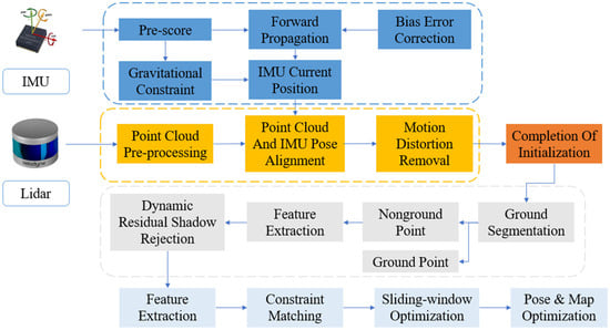
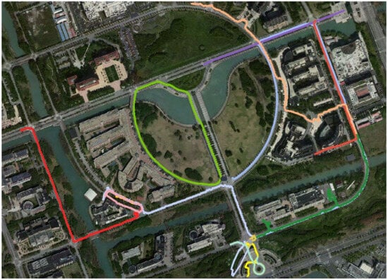
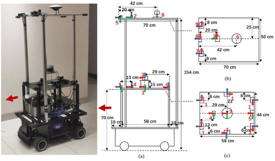
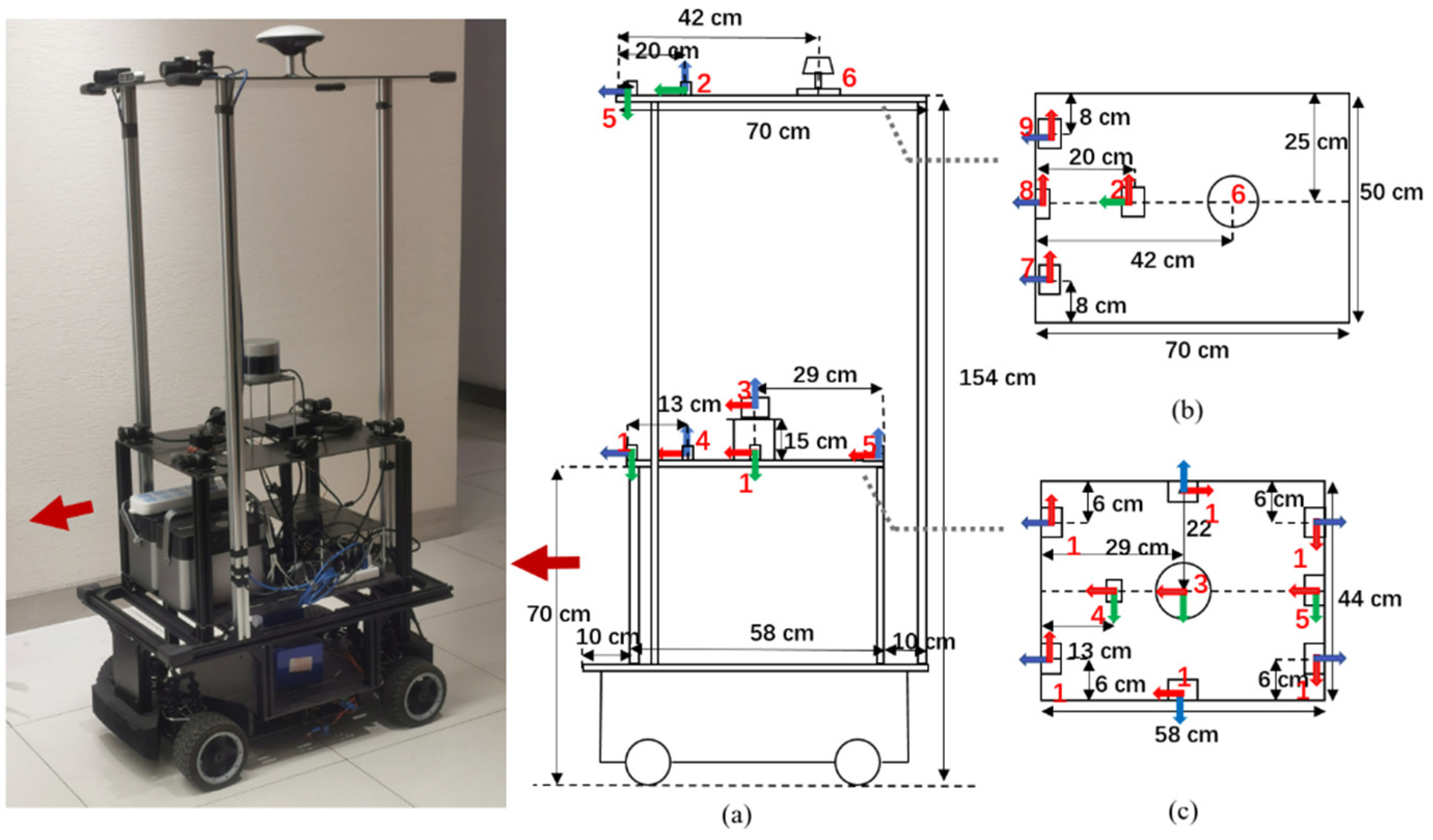
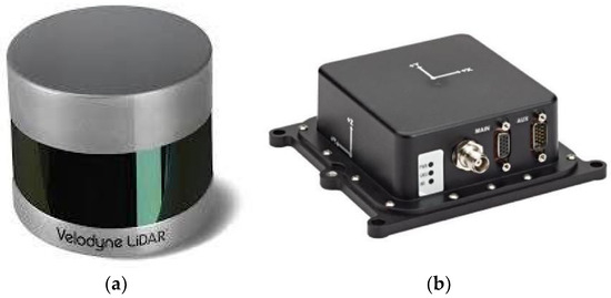
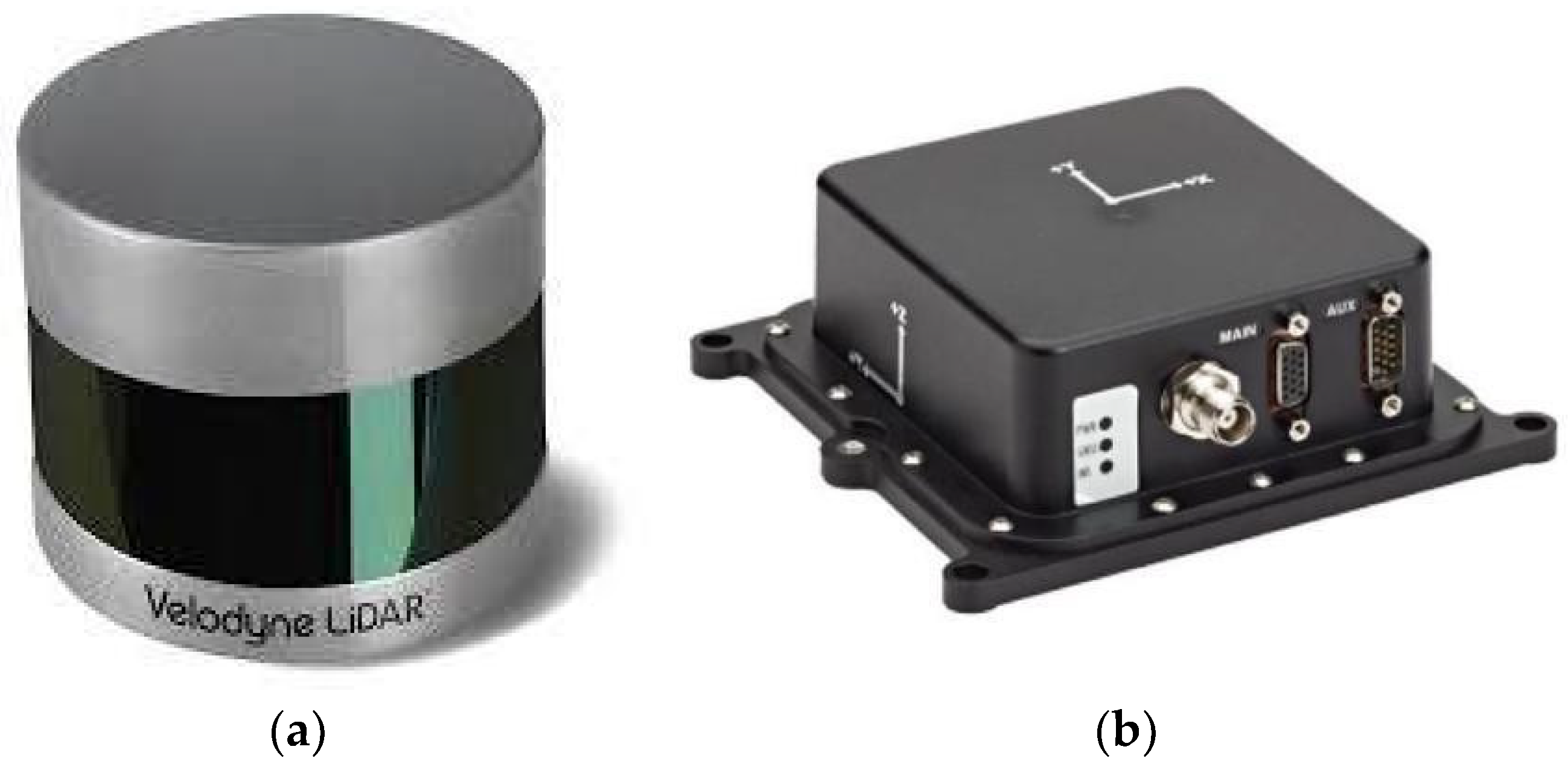
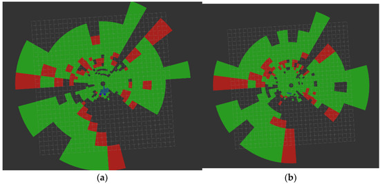
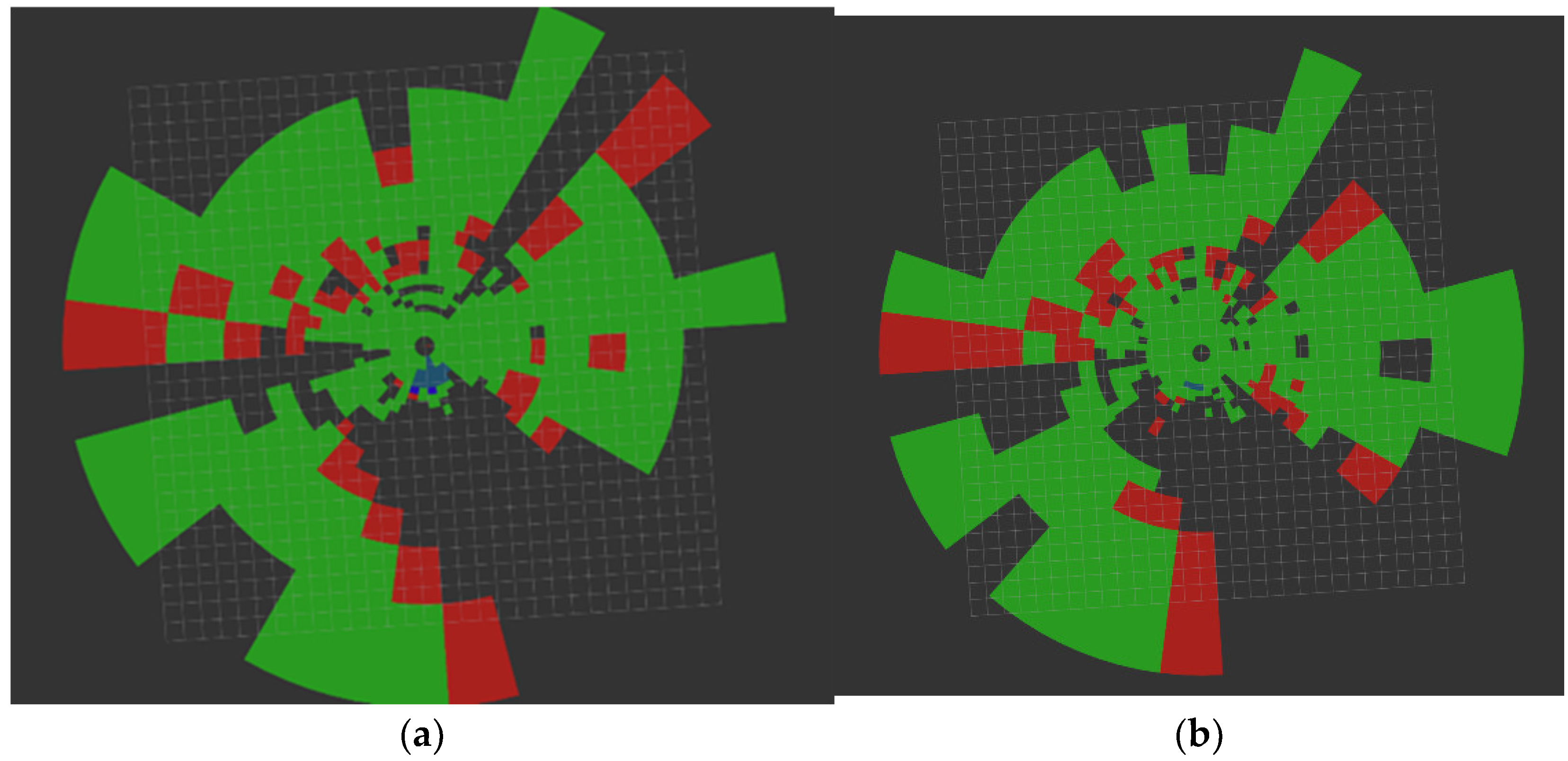
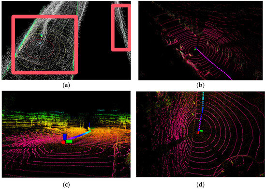
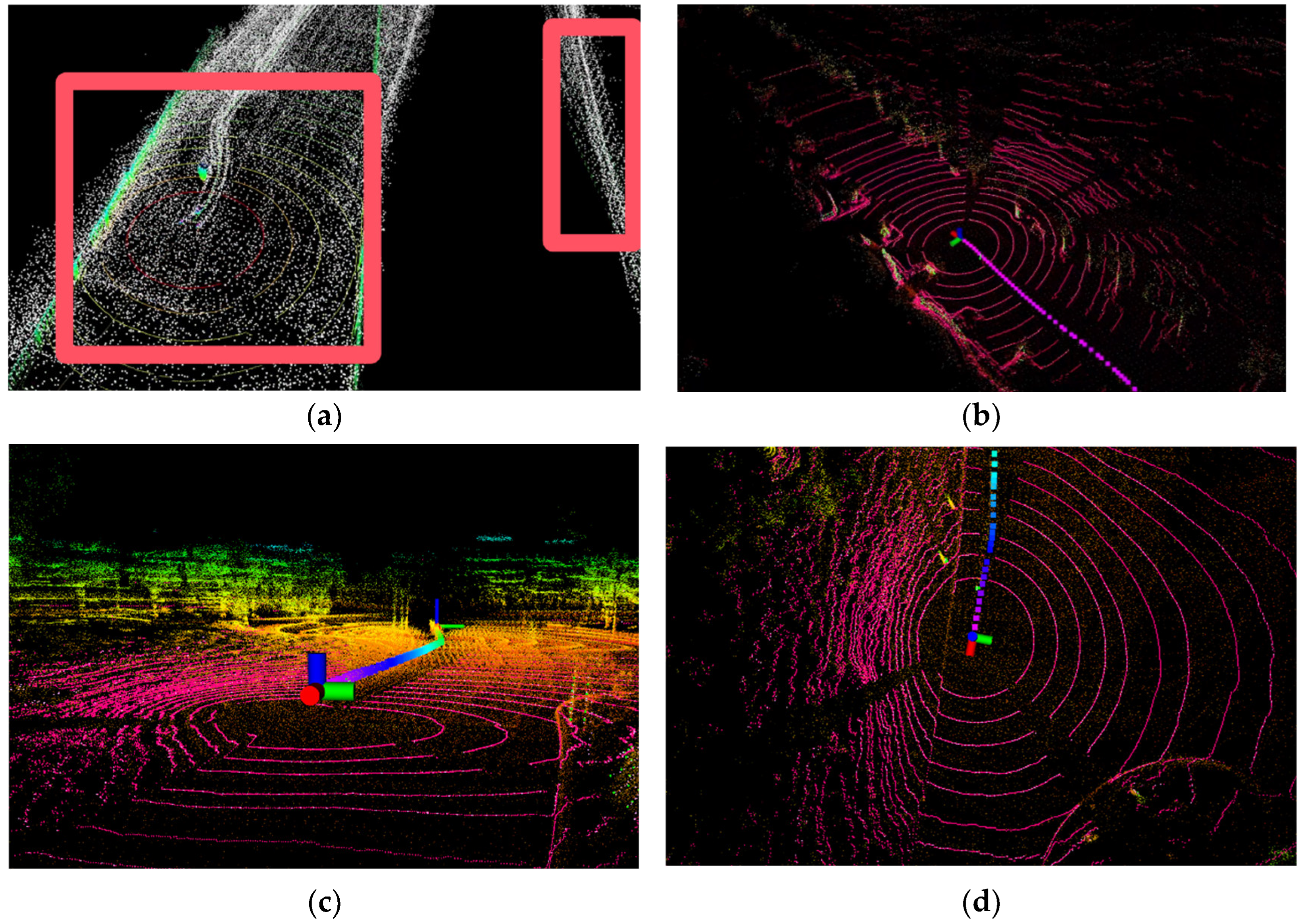
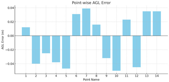
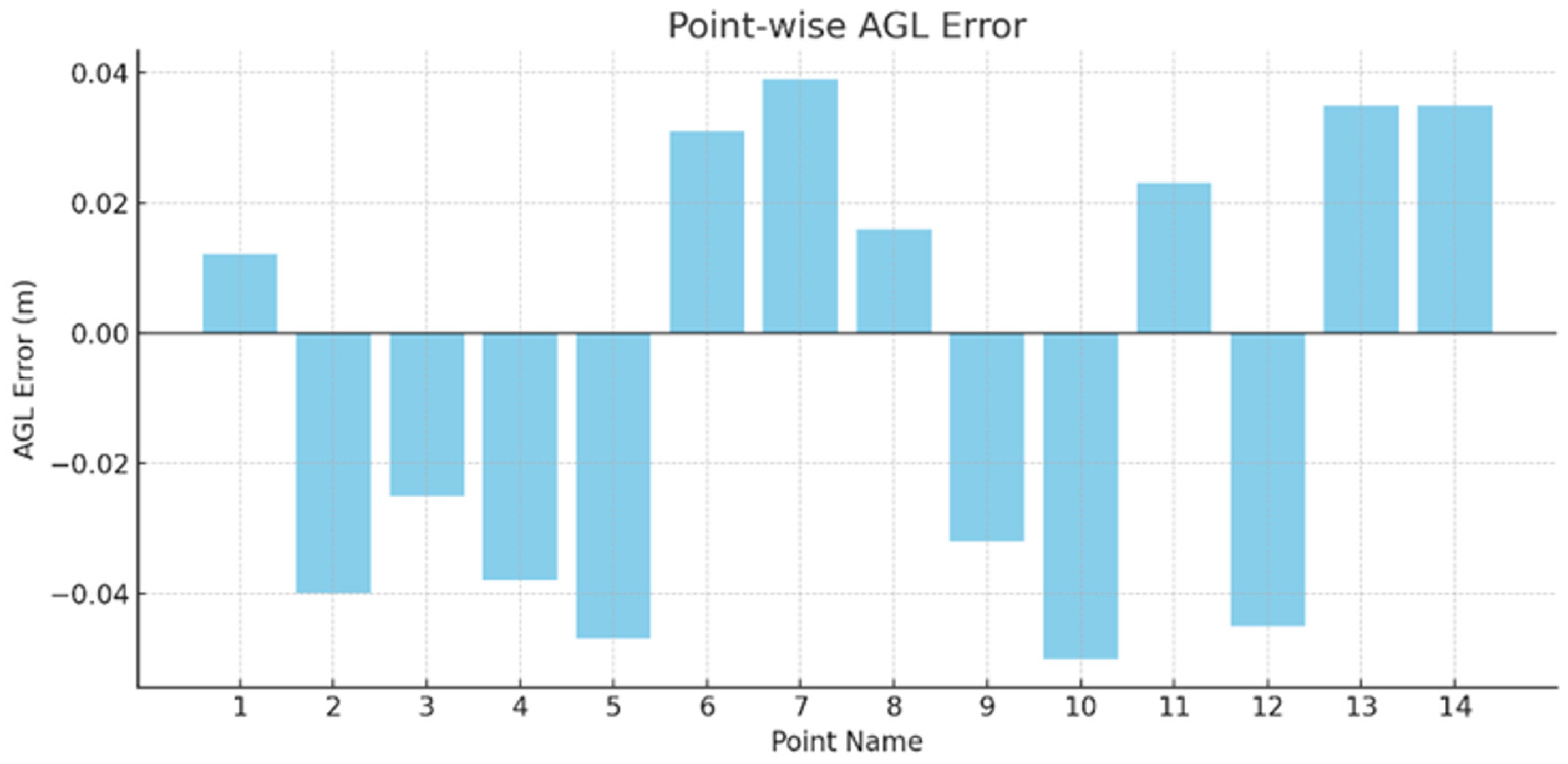
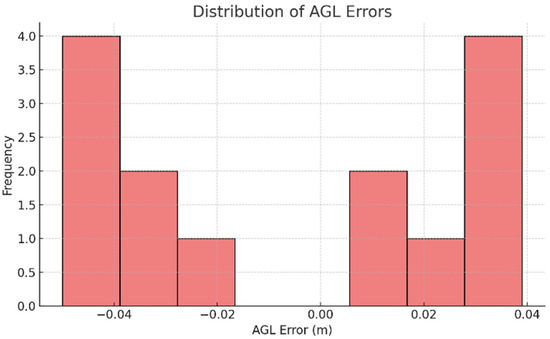
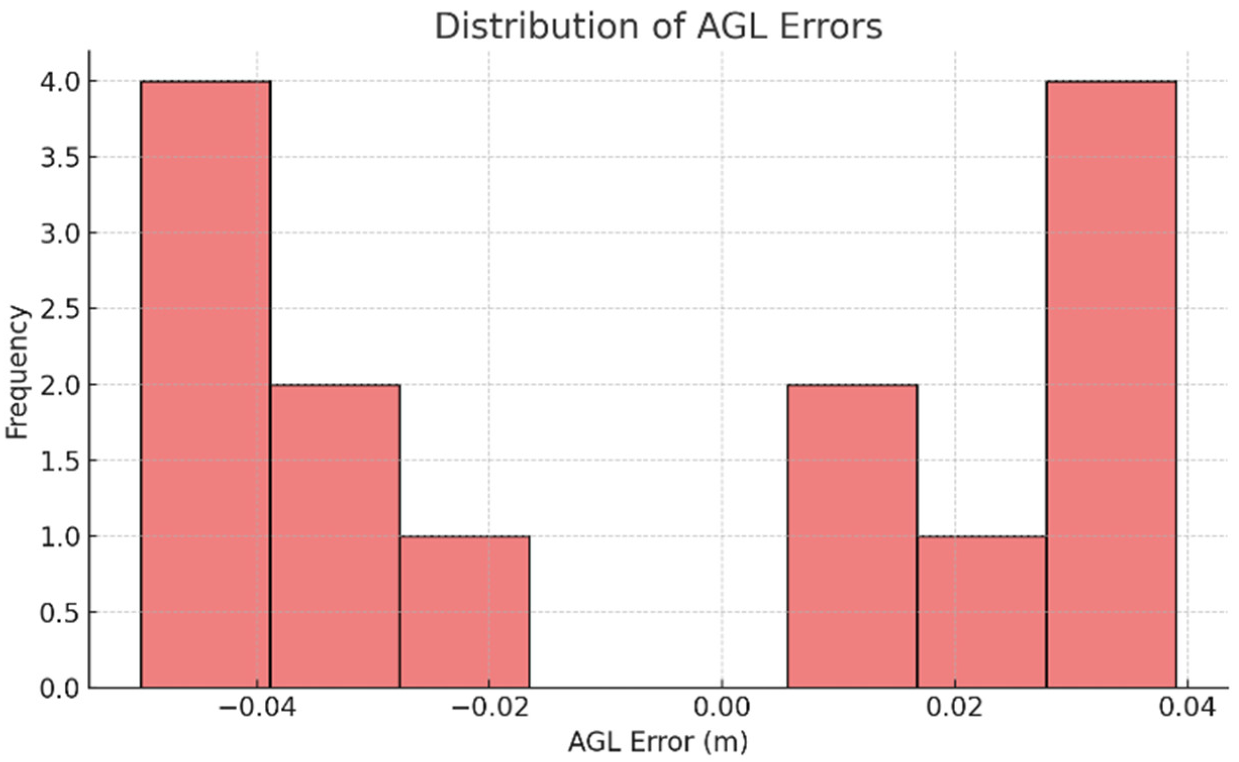
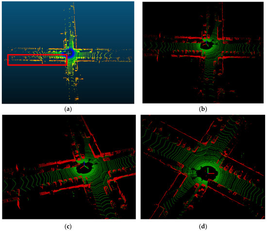
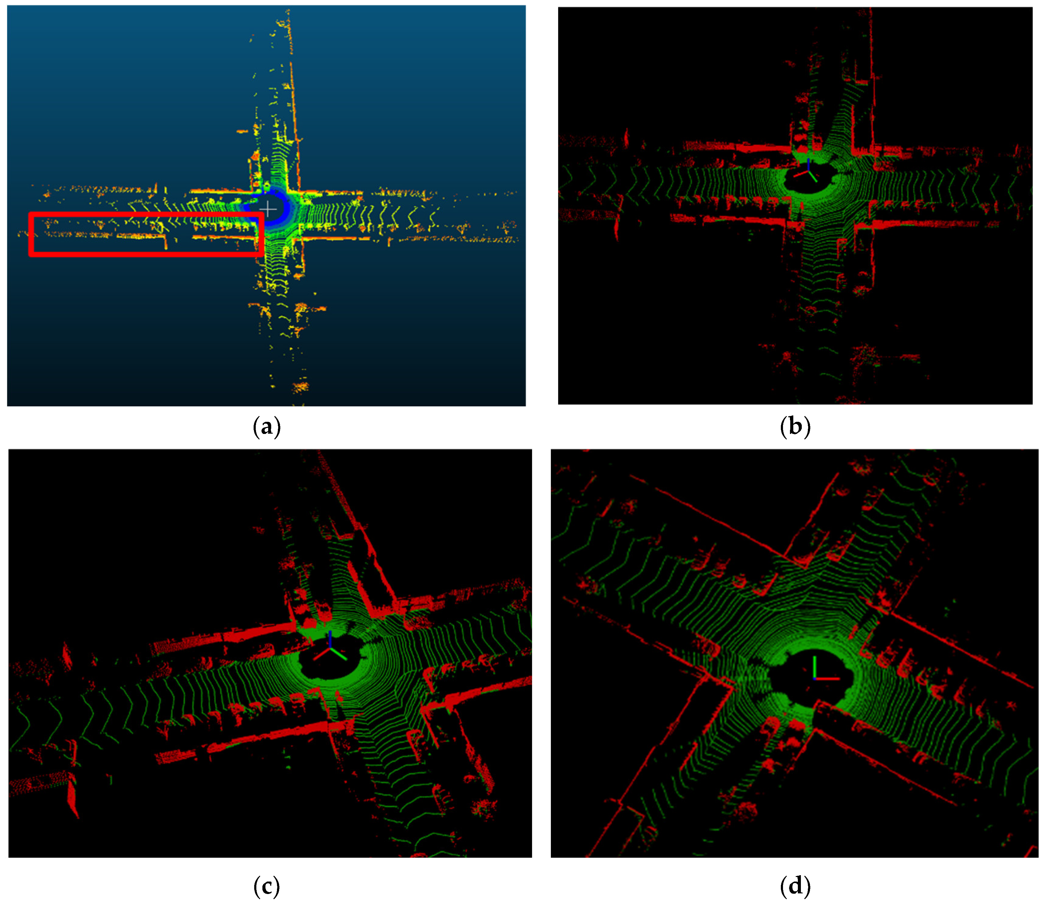
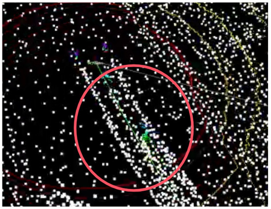
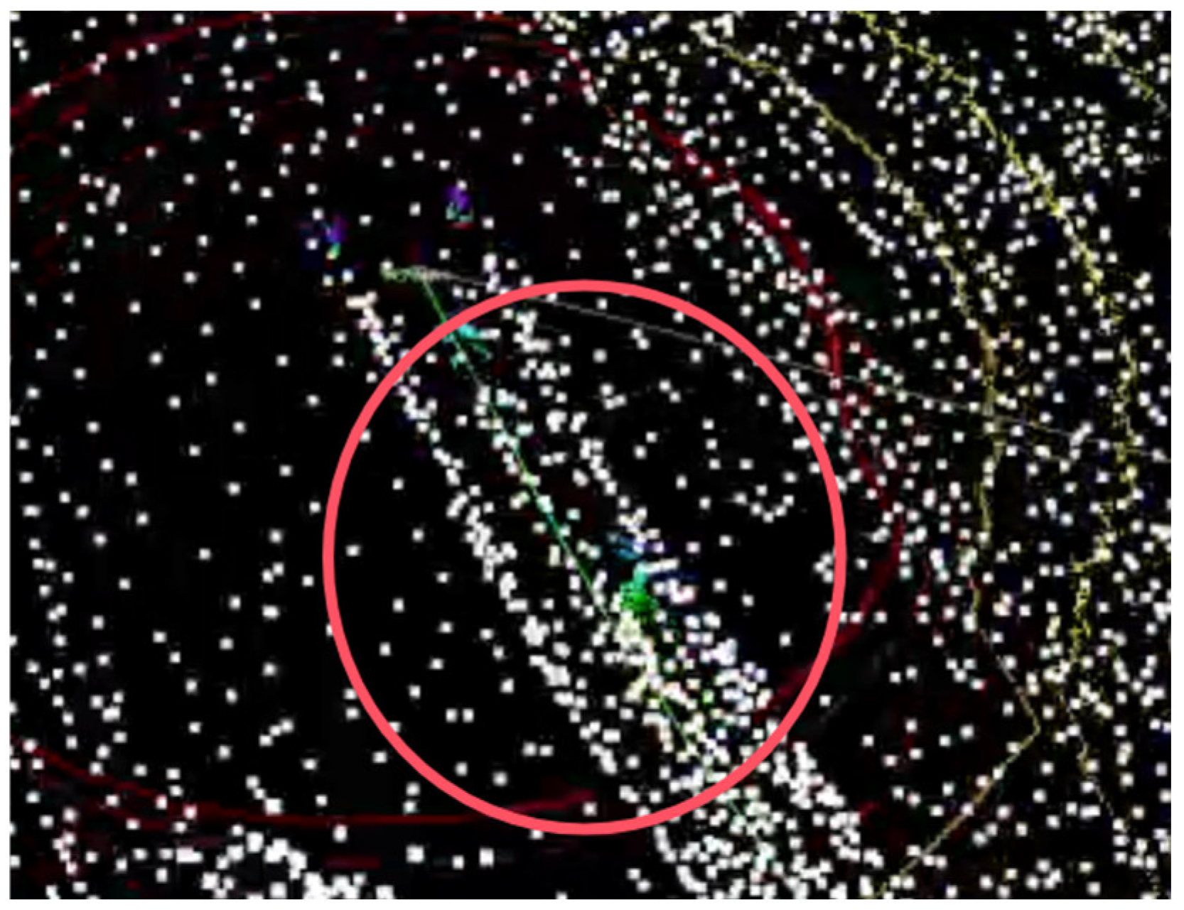
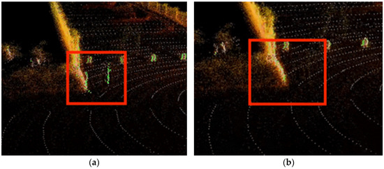
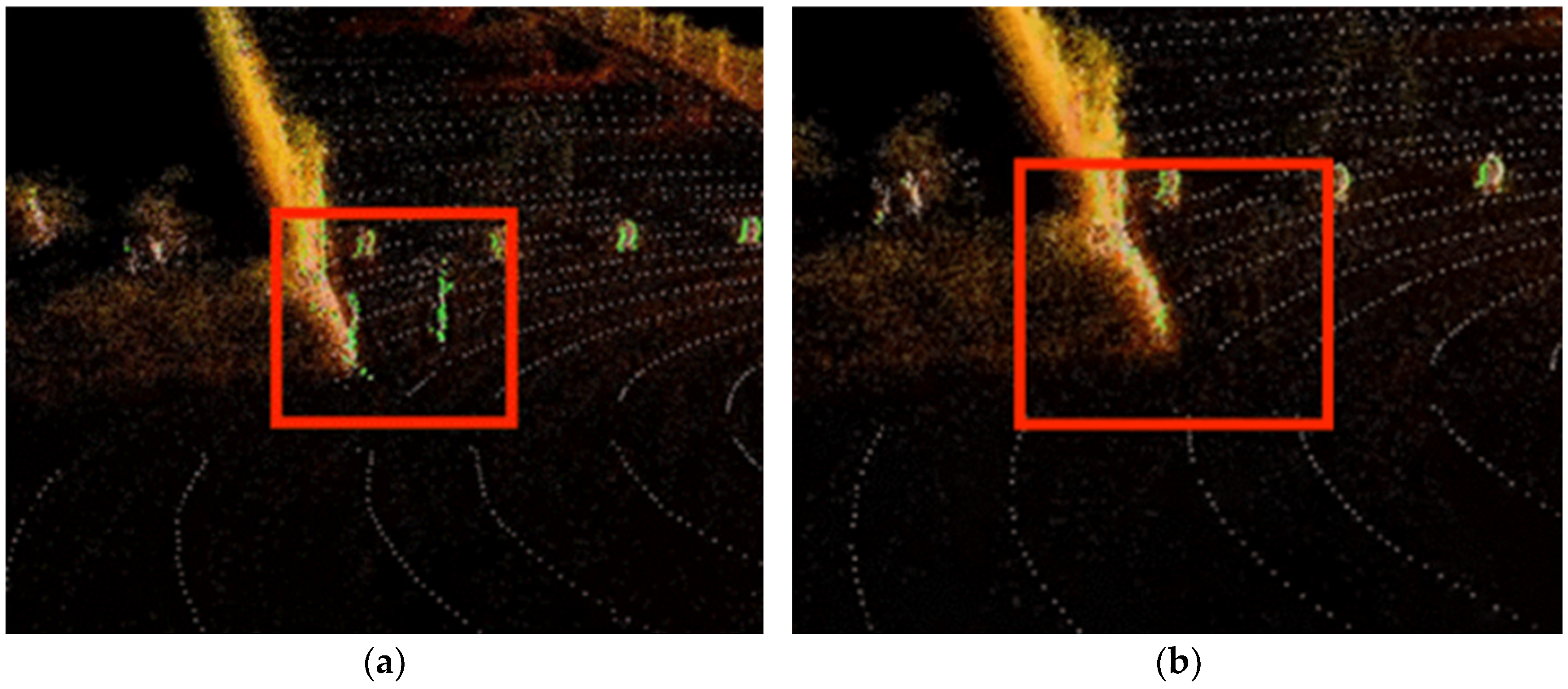
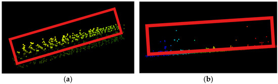
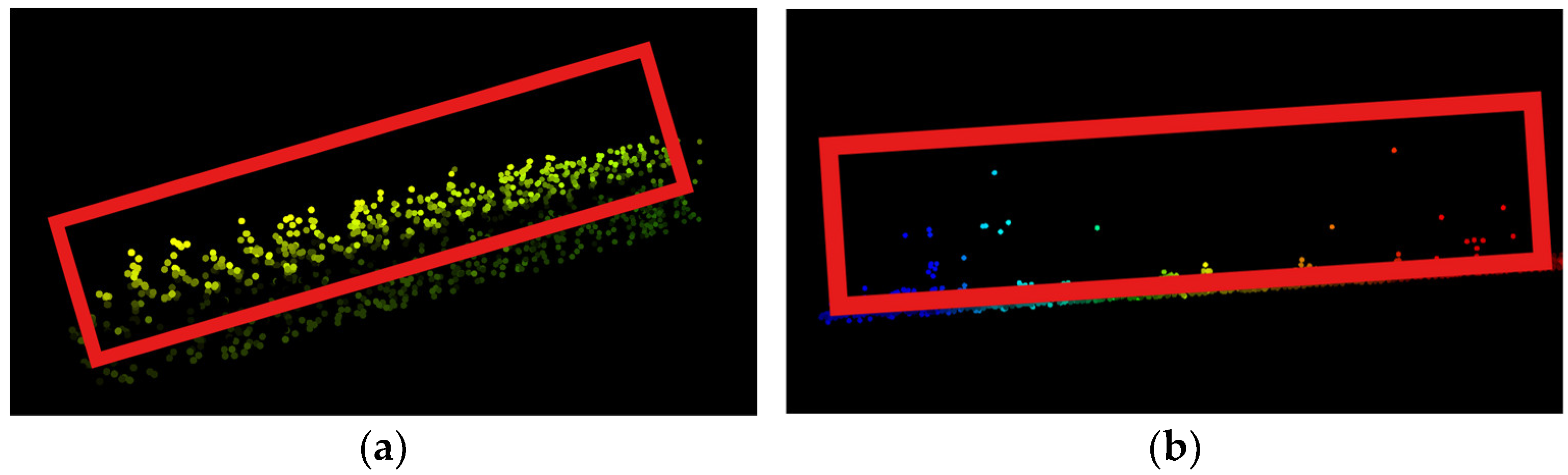
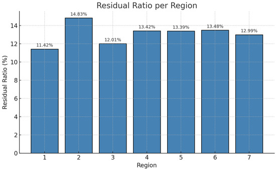
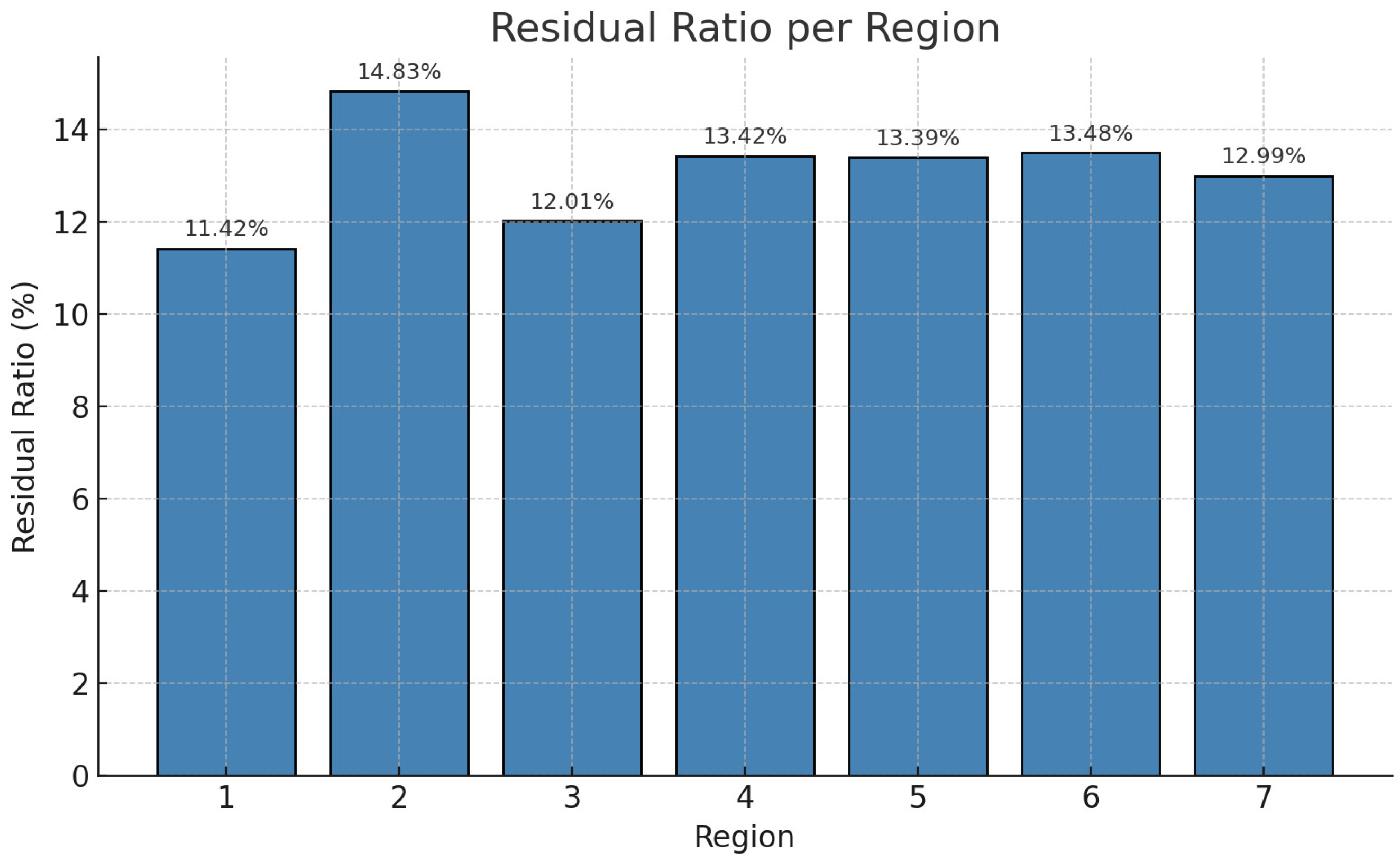
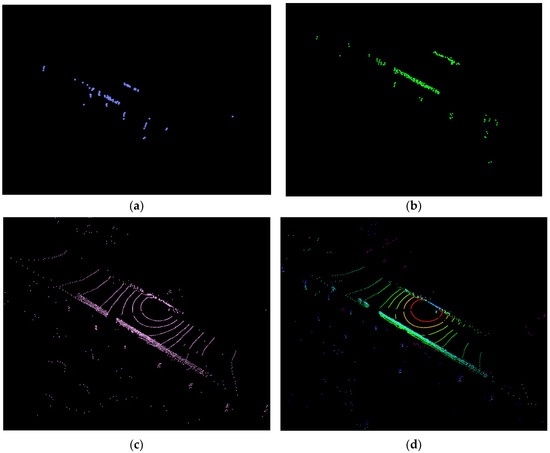
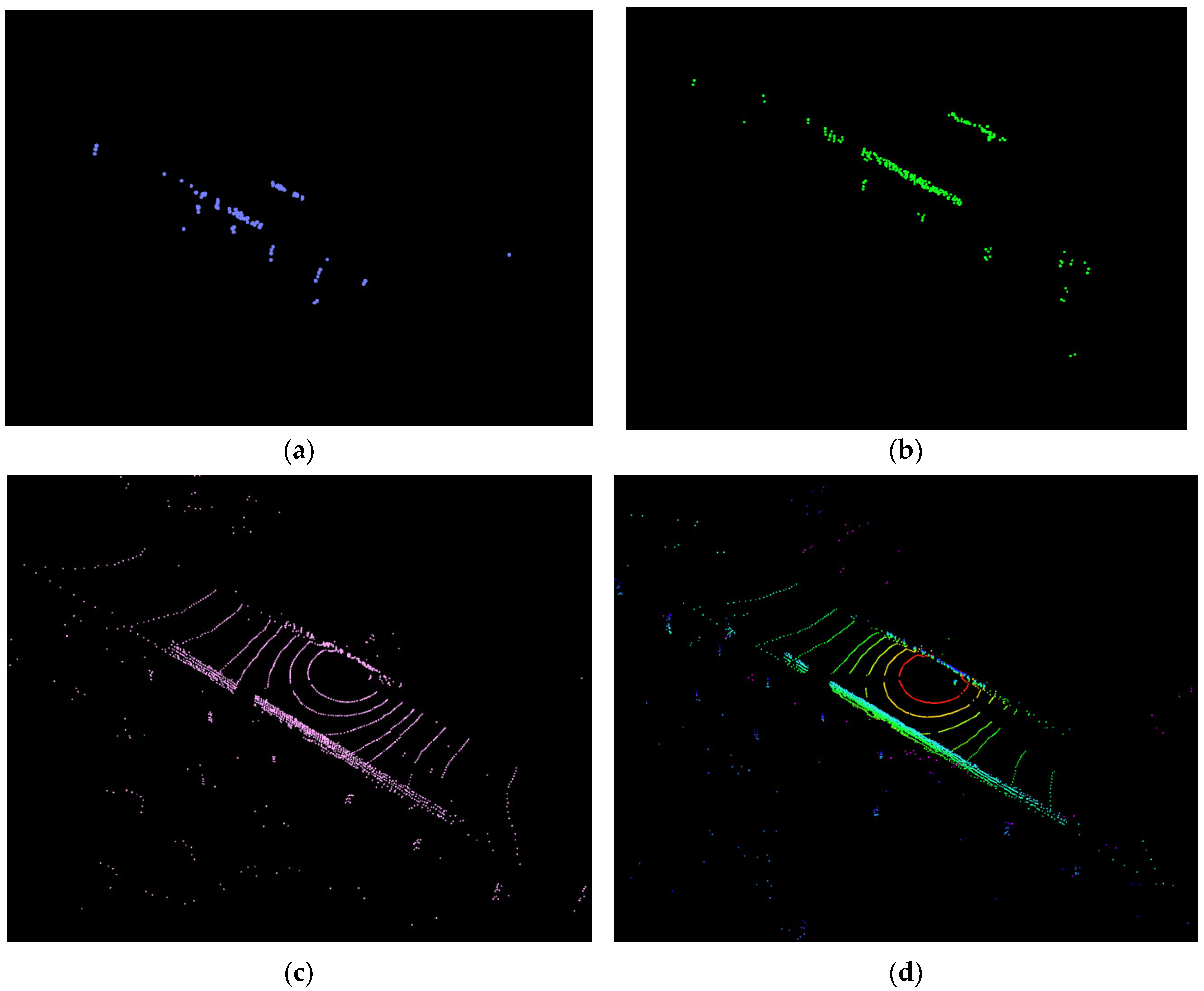
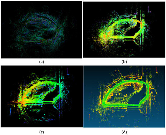
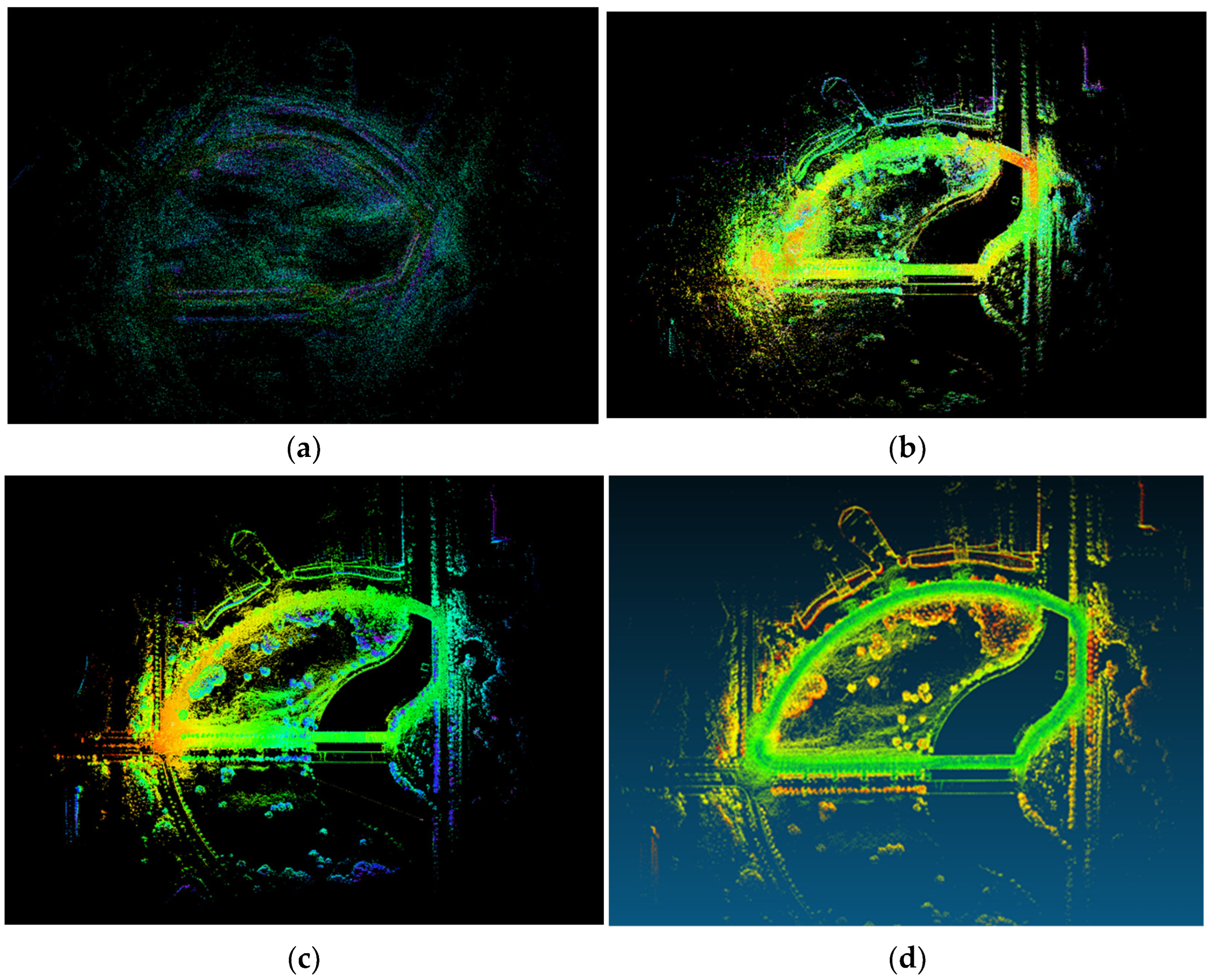
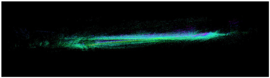
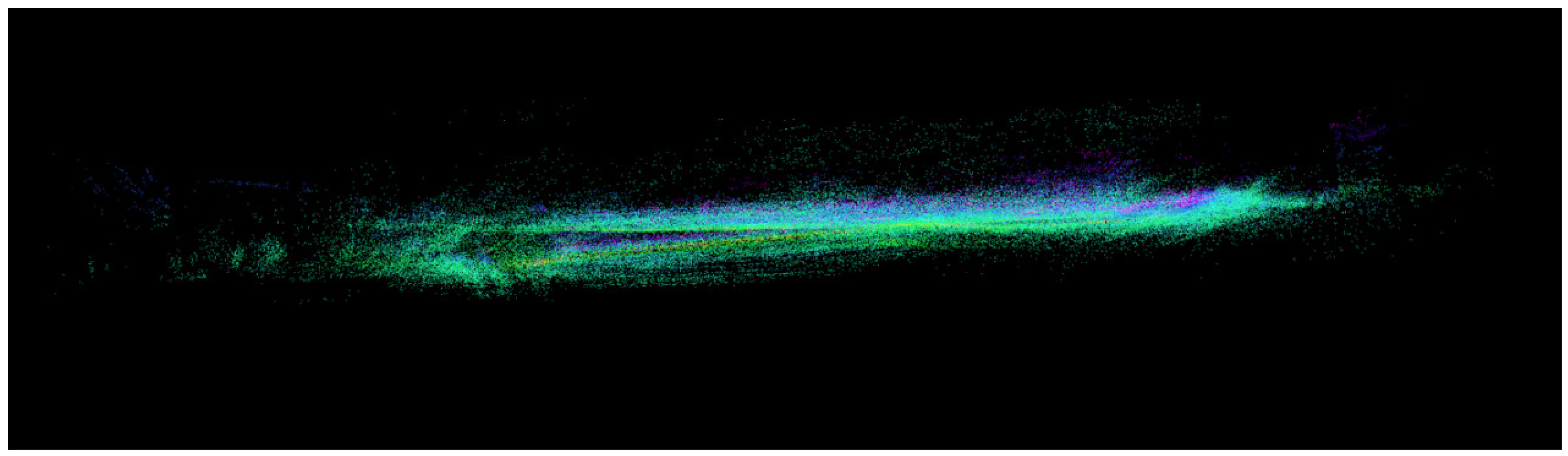
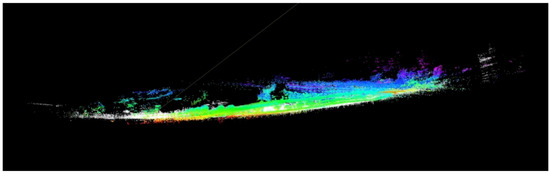
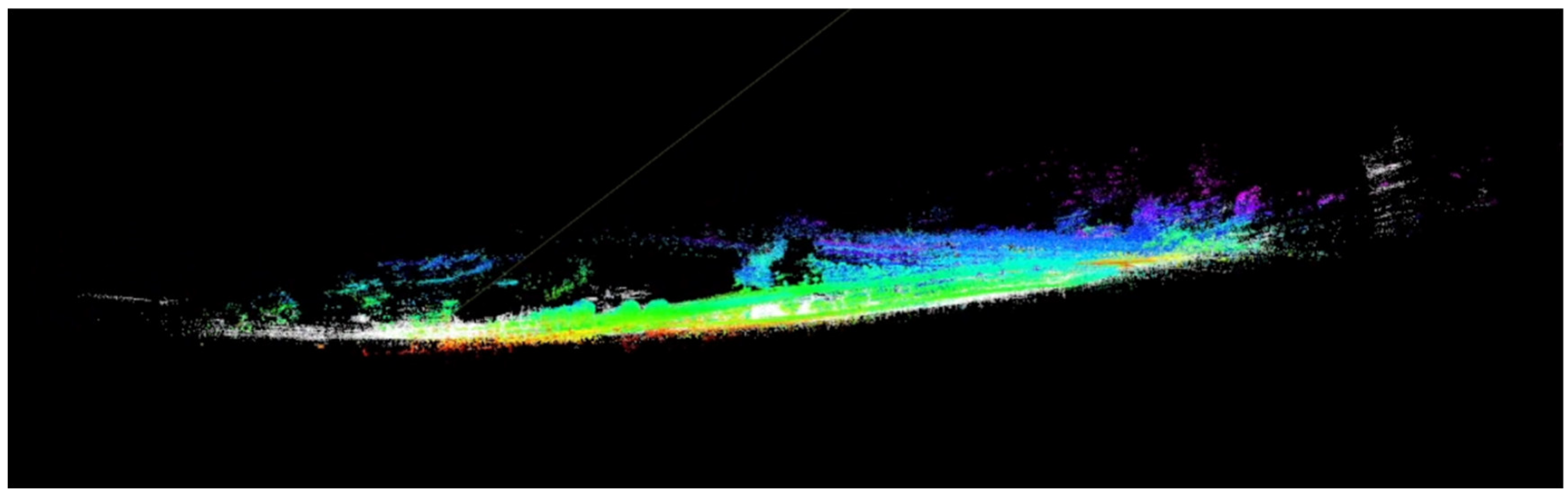
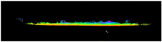
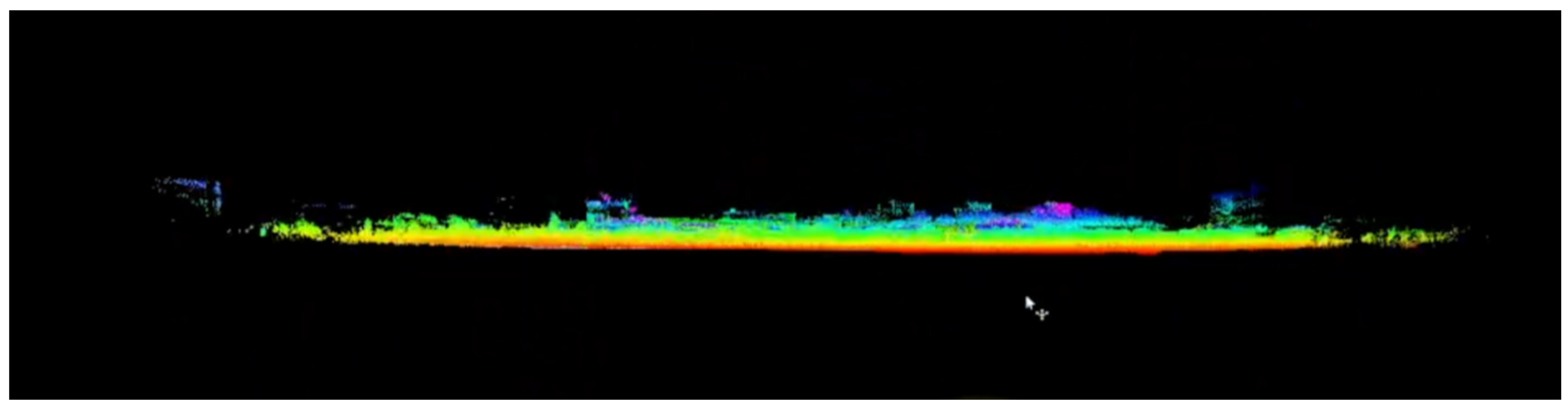
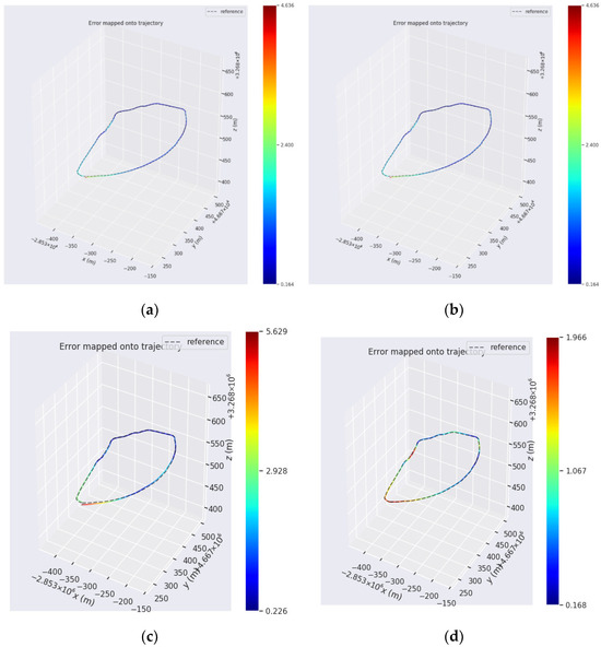
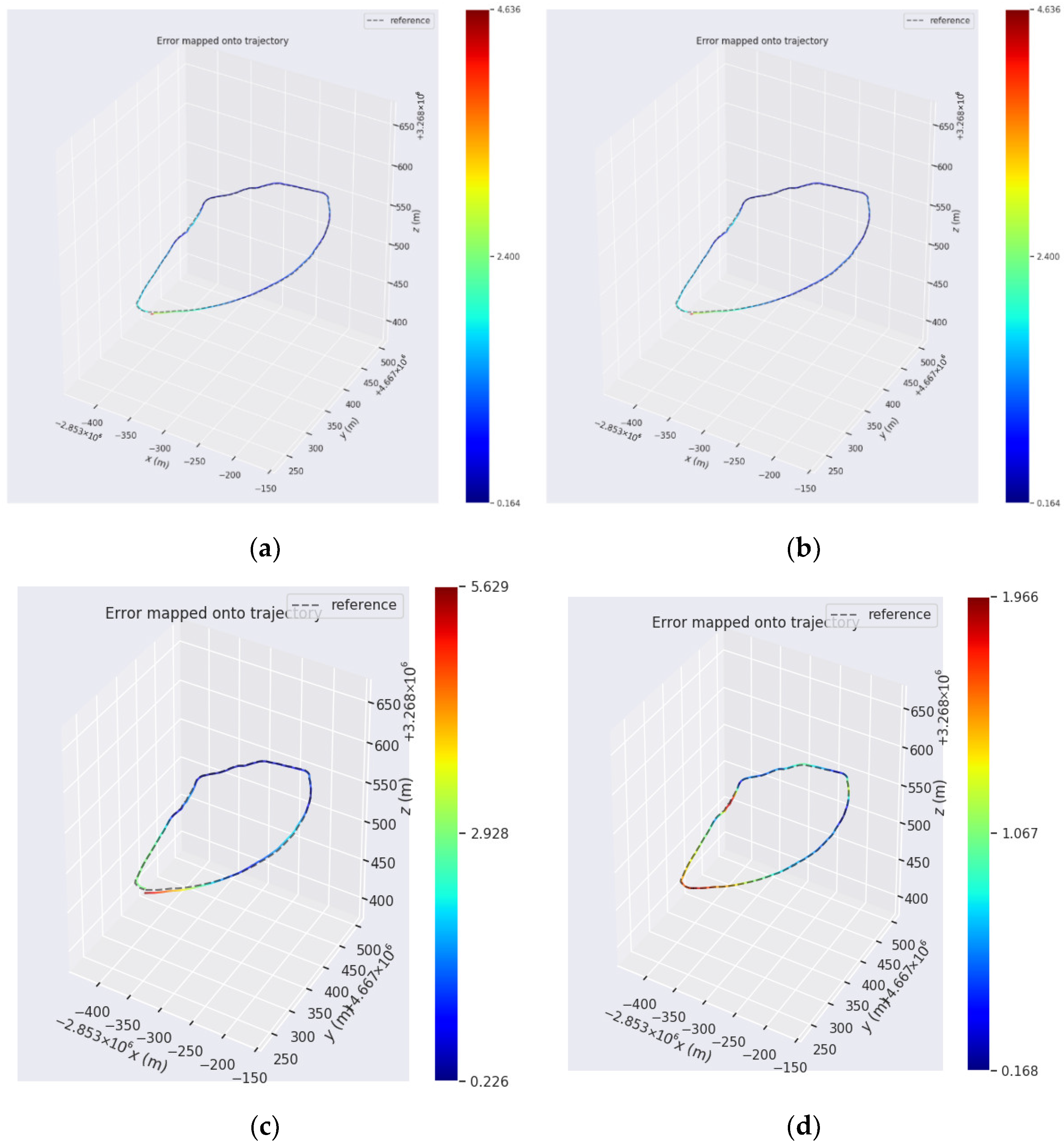
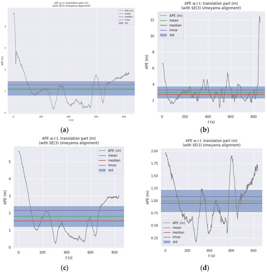
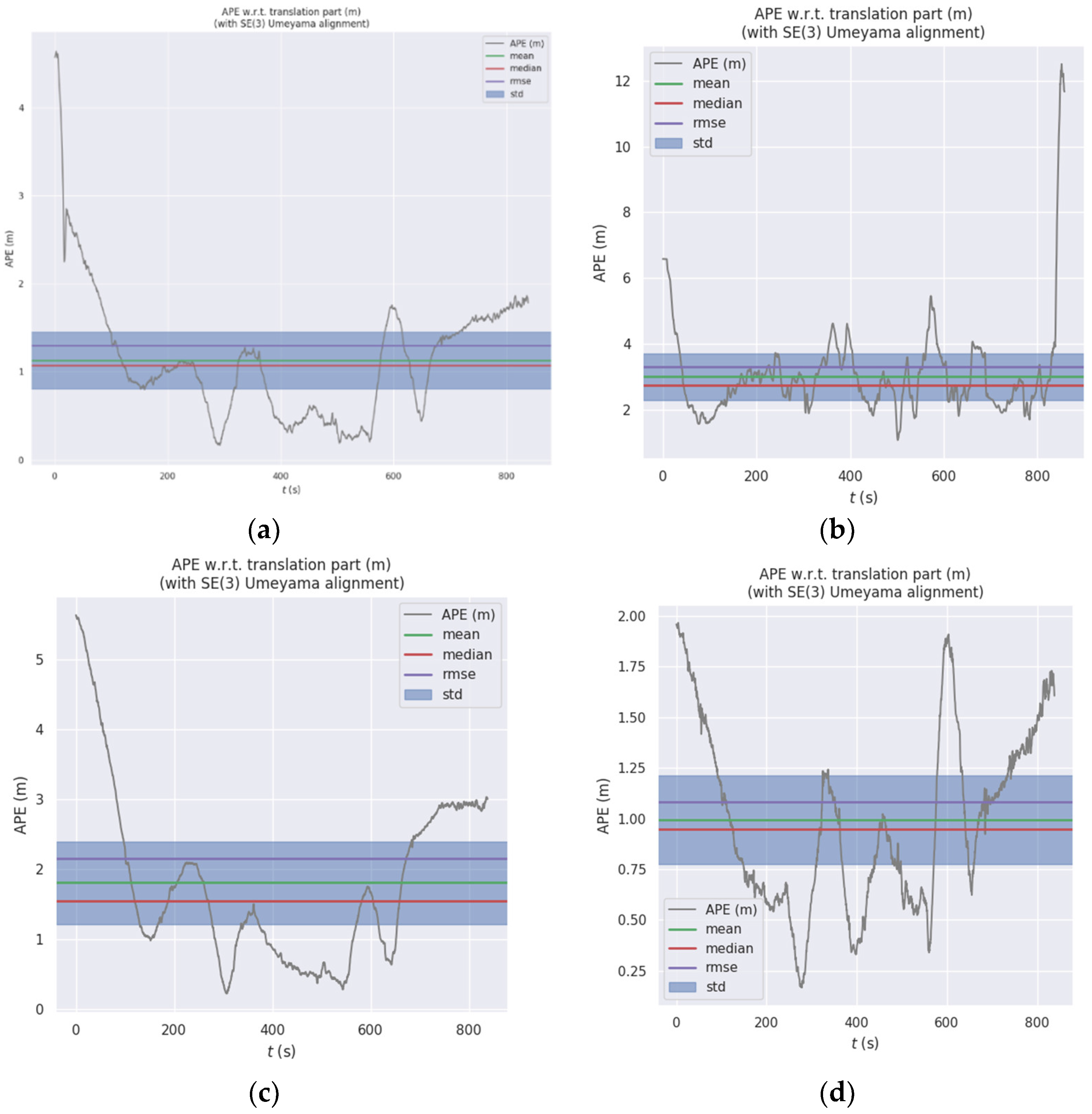
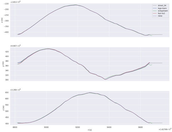
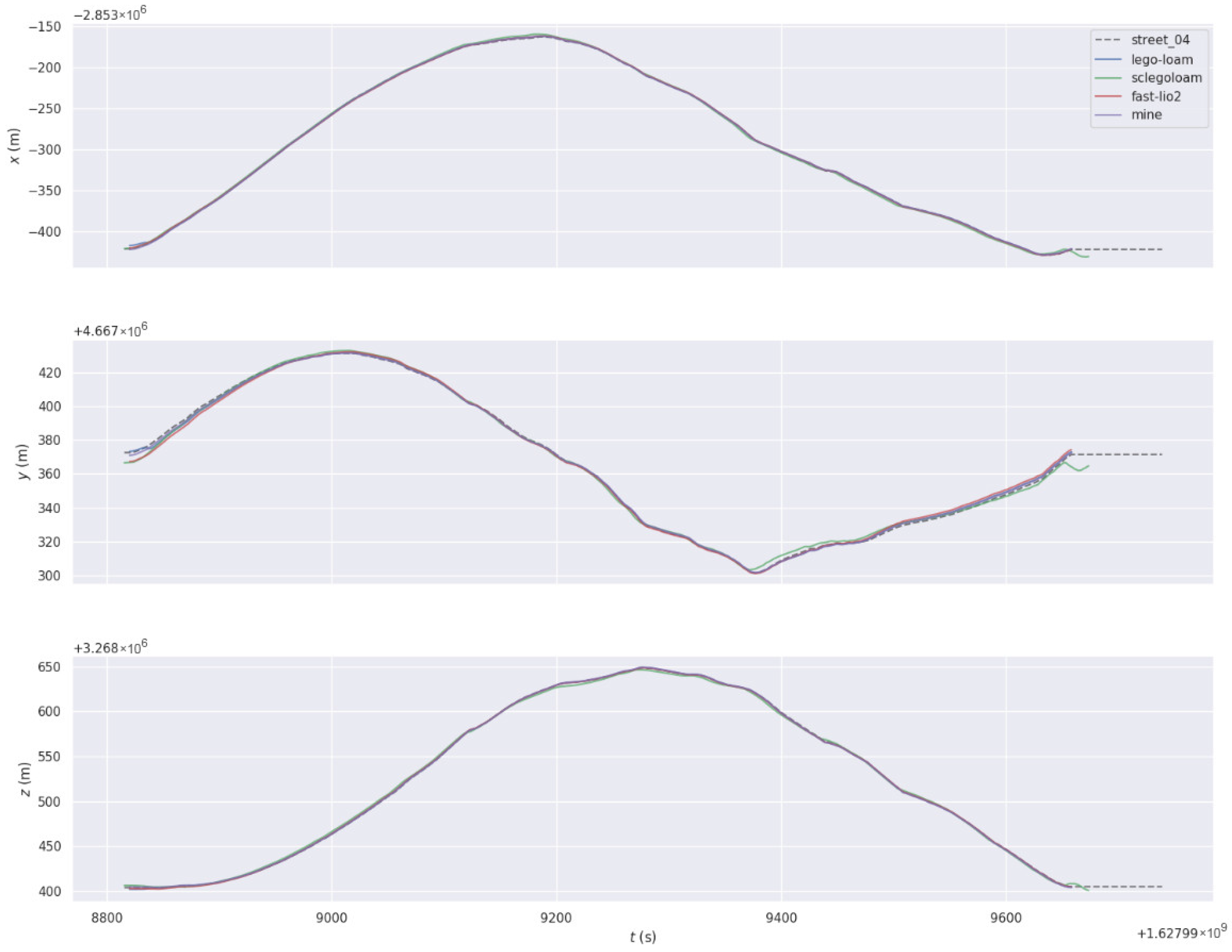

Disclaimer/Publisher’s Note: The statements, opinions and data contained in all publications are solely those of the individual author(s) and contributor(s) and not of MDPI and/or the editor(s). MDPI and/or the editor(s) disclaim responsibility for any injury to people or property resulting from any ideas, methods, instructions or products referred to in the content. |
© 2026 by the authors. Licensee MDPI, Basel, Switzerland. This article is an open access article distributed under the terms and conditions of the Creative Commons Attribution (CC BY) license.