Operator-Based Nonlinear Optimized Multi-Input Control Design and Its Application to a Vibrating Plate with Reduced-Sensor Implementation

Abstract

In nonlinear mechatronic systems with multiple coupled actuators, the allocation of control inputs affects both the feedback-system structure and the required actuator effort. This paper develops an operator-based nonlinear multi-input control framework within the robust right coprime factorization (RRCF) structure for systems with more actuator inputs than controlled outputs. The original multi-input plant is represented through a reduced-output formulation, and the control allocation is described by a mapping that selects a right inverse of the input-coupling. Specifically, the actuator inputs are determined by minimizing the quadratic voltage-based control-effort objective subject to the prescribed coupling relation and actuator constraints. Under the ideal allocation condition, the nominal Bezout Identity is preserved, while robust stability in the presence of plant perturbations, coupling uncertainty, and allocation errors is guaranteed when the generalized Lipschitz condition derived for the optimized RRCF system is satisfied. The proposed framework is applied to a vibrating plate actuated by multiple piezoelectric elements. For this application, the constrained two-input allocation problem is reduced to a scalar piecewise optimization problem and solved by a finite-candidate selection procedure. Comparative experiments show that the proposed approach achieves stronger vibration suppression, a lower voltage-based control-effort metric, and a more balanced allocation among the actuators. These results demonstrate the effectiveness of integrating constrained multi-input allocation with the operator-based robust control framework.

1. Introduction

Nonlinear control provides fundamental tools for the analysis and control of dynamical systems involving nonlinear behavior, uncertainties, and external disturbances [1,2,3]. In practical mechatronic systems, such difficulties may arise from nonlinear actuator characteristics, parameter variations, unmodeled dynamics, dynamic coupling, and external excitations, all of which can significantly affect closed-loop stability and performance [4,5]. These issues become particularly important in precision and flexible mechatronic systems, where multiple actuators and sensors interact through the structural dynamics. For systems employing piezoelectric actuators, nonlinear effects such as hysteresis, together with structural vibration and actuator interactions, further complicate the control design [6,7,8]. Consequently, robust nonlinear control methods capable of accommodating modeling uncertainties, external disturbances, and interactions among multiple control inputs remain important for practical mechatronic applications. Among the robust nonlinear control methodologies, the operator theory has also been implemented into nonlinear mechatronic systems in the form of a right coprime factorization (RCF) framework [9,10]. The operator-based nonlinear control approach focuses on the causal mapping from input to output, by which the overall feedback system has a bounded-input, bounded-output property [10,11]. The operator-based control strategy is applicable not only to single-input, single-output (SISO) systems [12,13], but also to multi-input, multi-output (MIMO) systems. Theoretical analyses within a MIMO control system were conducted in [14], and include consideration of internal couplings, robust stability and tracking performance. These analyses serve as the basis for further applications. In [15], a vibrating L-shaped manipulator was driven by two piezoelectric actuators from two parts, which was a controlled operator-based robust scheme. The soft actuator addressed in [16] was composed of multiple inputs to realize movement with three degrees of freedom, and the practical experiments were conducted given an M-SVR-based operator control system. However, the current methods require separate modeling of each actuator and the design of individual control systems, which lead to considerable computational complexity and design difficulty. In addition, the existing solution to coupling relies on feedback loops, which often introduce errors in practical engineering due to delays and noise.

Vibration control is an important topic in the field of mechatronics, and many studies have focused on this subject [17,18,19,20,21,22]. Specifically, this study addresses the problem of vibration control for a vibrating plate structure, which can be commonly seen in various fields like mechanical, civil, and aerospace engineering, among others. The vibrating plate was depicted mathematically in [23]. To meet the requirement of lower cost and mass of mechanical systems, the vibration control on such items was conducted using piezoelectric devices serving as both actuators and sensors. However, the hysteresis property of piezoelectric actuators caused difficulty and challenges in control system design. To overcome this issue, the Prandtl–Ishlinskii model [24,25] was selected to describe the hysteresis dynamics. Subsequently, given the physical model of the vibrating plate and hysteresis model, an operator-based nonlinear control design was established in [23]. Although the experimental results suggest satisfactory performance, this work was not extended to the MIMO scenario. In contrast, the actuators and sensors were divided into two groups, as noted in [26,27], by which the vibration control for the vibrating plate was realized from two dimensions. Although the coupling was considered with compensation, the stability of the designed right coprime factorization feedback system was not concisely derived [26]. Moreover, the unbalanced multi-input allocation [27] may result in unnecessary energy consumption, and the resonance frequency-based compensation [26] introduced additional computational complexity.

Motivated by the aforementioned problems, the main contributions of this work are summarized as follows: (1) While existing studies have considered operator-based RRCF design and multi-input optimization separately, their integration is developed in this paper. In particular, the optimization process is interpreted from a mapping perspective, under which the resulting RRCF feedback system is shown to remain robustly stable in the presence of various perturbations, including coupling inaccuracies and optimization errors. (2) The proposed optimized RRCF feedback framework is implemented on a vibrating plate system. The framework enables a low-cost experimental design by reducing the number of required sensors. Comparative results further demonstrate improved vibration-suppression performance together with a more balanced multi-input allocation.

The outline of this paper is as follows. Section 2 offers mathematical preliminaries on operator theory and RRCF feedback system. Section 3 provides the decoupling approach and the optimized RRCF feedback control design. The practical verification is exhibited in Section 4, where the proposed framework is applied into an vibrating plate system to realize vibration suppression control. Eventually, the whole work is concluded in Section 5.

2. Mathematical Preliminaries of Operator-Based RRCF Systems

In this work, the operator-based optimized nonlinear system design is conducted within the basic scheme of an RRCF feedback system, which will be briefly introduced as follows.

Initially, the introduction starts from the notations of spaces and operators. Let $\mathit{U}$ be the linear space of measurable functions $\mathit{u}:[0,\infty )\to {\mathbb{R}}^m$. For each constant ${\mathit{t}}_0\in [0,\infty )$, the truncations of $\mathit{u}$ is introduced as follows:

$${\mathit{u}}_{t_0}\left(t\right):=\left\{\begin{array}{cc}\mathit{u}\left(t\right),\hfill & \mathrm{if}t\in [0,t_0],\hfill \\ 0,\hfill & \mathrm{if}t\in (t_0,\infty )\hfill \end{array}\right.$$

A Banach space ${\mathit{U}}_B\subset U$ is defined with a norm ${\parallel ·\parallel }_{U_B}$, which denotes the supremum norm on $U_B$. Define

$$U^e=\left\{\mathit{u}\in U:\parallel {\mathit{u}}_{t_0}{\parallel }_{U_B}<\infty \mathrm{for}\mathrm{all}{t}_0<\infty \right\}.$$

Here ${\mathit{U}}^e$ is a linear subspace of $\mathit{U}$. The space ${\mathit{U}}^e$ so defined is called the extended linear space associated with the Banach space ${\mathit{U}}_B$ [11]. Moreover, let ${\mathit{U}}_s$ be the stable subspace of $\mathit{U}$, and in this paper, it is assumed that ${\mathit{U}}_s$ is a proper nontrivial linear subspace of $U^e$ and $\mathit{U}\setminus U_s\ne Ø$ [9]. Analogously, let $\mathit{Y}$ be the linear space of measurable functions $\mathit{y}$, and ${\mathit{Y}}_s$ be the stable subspace of $\mathit{Y}$.

Given the aforementioned definitions of spaces, a given nonlinear nominal plant $y\left(t\right)=\Phi \left(u\right)\left(t\right)$ is interpreted as an operator, namely, $\Phi :\mathit{U}\to Y$, which is the mapping from $\mathit{U}$ towards $\mathit{Y}$. In this sense, a stable operator (mapping) is defined as follows.

Definition 1 

([9]). An operator $\Phi :\mathit{U}\to Y$ is said to be stable if $\Phi \left(U_s\right)\subseteq Y_s$.

It should be noted that the specific definitions of ${\mathit{U}}_s$ and ${\mathit{Y}}_s$ may depend on the physical constraints in real-world scenarios. For simplicity, nominal notations ${\mathit{U}}_s$ and ${\mathit{Y}}_s$ are thus used here.

In addition, let $\Psi (U,Y)$ be the set of stable operators mapping from $\mathit{U}$ towards $\mathit{Y}$. Then $\Psi (U,Y)$ contains a subset defined as

$$\mathcal{U}(U,Y)=\{M:M\in \Psi (U,Y), M \mathrm{is} \mathrm{invertible} \mathrm{with} M^{-1}\in \Psi (U,Y)\}$$

and the elements of $\mathcal{U}(U,Y)$ are named as unimodular operators [9,10].

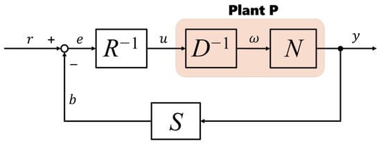
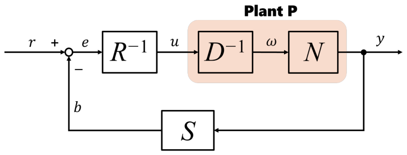
Next, the basic schemes of operator-based RRCF feedback systems are provided. Generally, the nonlinear right coprime factorization (RCF) feedback system can be depicted as in Figure 1. Specifically, $\mathit{P}:U\to Y$ denotes the objective plant, which is possibly unstable. $\mathit{u}\in U$ and $\mathit{y}\in Y$ denote the input and output of $\mathit{P}$, respectively. $\mathit{N}:W\to Y$ and ${\mathit{D}}^{-1}:U\to W$ serve as the right factorization of $\mathit{P}$, which can be formulated as $\mathit{P}=N{D}^{-1}$. ${\mathit{D}}^{-1}$ is a potentially unstable operator, while $\mathit{N}$ and $\mathit{D}$ are stable operators. Note that the signal $\omega \in W$ is defined as the quasi-state of $\mathit{P}$, and space $\mathit{W}$ is the quasi-space. In addition, two controllers $b=\mathit{S}\left(y\right)$ and $e=\mathit{R}\left(u\right)$ are designed, by which the feedback system can be said to be bounded-input, bounded-output (BIBO) stable if the following lemma is satisfied.

Figure 1. Basic scheme of the nonlinear RCF feedback system.

Lemma 1 

([9]). For a nonlinear feedback system, shown in Figure 1, where $\mathit{N}$ and ${\mathit{D}}^{-1}$ are the right factorization of $\mathit{P}$, the overall system can be defined as the right coprime factorization of $\mathit{P}$ if the Bezout Identity

$$SN+RD=M,M\in \mathcal{U}(W,U)$$

(1)

is satisfied. Moreover, the overall system satisfying (1) is said to be BIBO stable.

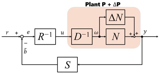
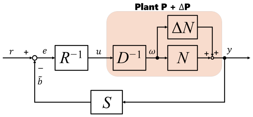
Hence, one can find $\mathit{r}=M\left(\omega \right)$ and the operator $\mathit{M}$ in the Bezout Identity (1) is required to be unimodular, by which the stability of both plant $\mathit{P}$ and the overall RCF feedback system are confirmed. Next, consider the existence of bounded perturbation $\Delta P$, which can be factorized into $\Delta N$ as shown in Figure 2. Hence, one can write $\mathit{P}+\Delta P=(N+\Delta N)D^{-1}$.

Figure 2. Basic scheme of the nonlinear RRCF feedback system.

In this sense, the perturbed Bezout Identity can be rewritten as

$$S(N+\Delta N)+RD=\tilde{M}.$$

However, one can find that the bounded $\mathit{N}+\Delta N$ does not always result in unimodular $\tilde{M}$, by which the robust stability of perturbed feedback system in Figure 2 is undetermined. To address this issue, a robust condition was proposed in [10] and is cited as follows.

Lemma 2. 

Let ${\mathcal{D}}^e$ be a linear subspace of the extended linear space ${\mathit{U}}^e$ associated with the Banach space ${\mathit{U}}_B$. Let ${\mathcal{D}}^e$ be a stable subspace of $\mathit{U}$. Consider a perturbed feedback system shown in Figure 2, where the Bezout Identity for a nominal plant holds as $\mathit{S}N+RD=M$. The perturbed feedback system is stable if

$$\parallel (S(N+\Delta N)-SN)M^{-1}{\parallel }_{\mathcal{L}}<1$$

(2)

is satisfied for any $\mathit{r}\in {\mathcal{D}}^e$.

The norm ${\parallel ·\parallel }_{\mathcal{L}}$ in (2) is defined as the generalized Lipschitz semi-norm [10,11], which is formulated as

$${\parallel Q\parallel }_{\mathcal{L}}=\underset{T\in [0,\infty )}{\sup }\underset{\begin{array}{c}u,\tilde{u}\in {\mathcal{D}}^e\\ u_T\ne {\tilde{u}}_T\end{array}}{\sup }{\displaystyle \frac{{\parallel \left[Q\left(u\right)\right]}_T-{\left[Q\left(\tilde{u}\right)\right]}_T{\parallel }_{Y_B}}{\parallel u_T-{\tilde{u}}_T{\parallel }_{U_B}}}$$

(3)

where $\mathit{Q}:U\to Y$ is a nominal stable operator.

3. Optimized RRCF Feedback Control Design

In this section, theoretical improvement on RRCF feedback systems considering multi-input optimization is presented. The decoupling approach is initially described, followed by the stability and robustness analysis of the proposed control system design.

3.1. Decoupling Approach

In this work, the multi-input nonlinear mechatronic system is addressed, which can be interpreted as operators and denoted as

$$y\left(t\right)=P\left(u\right)\left(t\right)$$

(4)

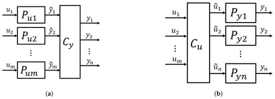
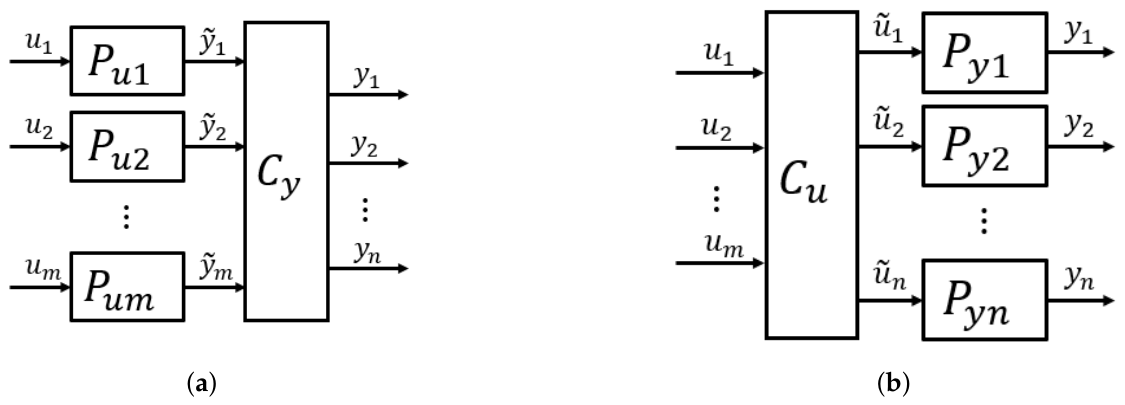
where $u\left(t\right)\in {\mathbb{R}}^m:\{u_1,u_2,\dots ,u_m\}$ and $y\left(t\right)\in {\mathbb{R}}^n:\{y_1,y_2,\dots ,y_n\}$, $\mathit{m}\ge n$. According to the existing operator-based RRCF control schemes [10], the objective system $\mathit{P}$ is generally divided into ${\mathit{P}}_{u1},{\mathit{P}}_{u2},\dots ,P_{um}$ corresponding to the dimension of inputs, by which the RCF of ${\mathit{P}}_{u1},{\mathit{P}}_{u2},\dots ,P_{um}$ can be conducted individually. Such an approach is depicted in Figure 3a, where ${\mathit{C}}_y$ denotes the mapping from individual output ${\tilde{y}}_1,\dots ,{\tilde{y}}_m$ to overall output, together with potential mutual coupling.

Figure 3. Decoupling approaches for $\mathit{P}$ according to different dimensions: (a) Input-based decoupling; (b) output-based decoupling.

Although some real-world applications of the approach based on ${\mathit{C}}_y$ have been conducted, the computational complexity caused by higher dimensions ($\mathit{m}\ge n$) and the difficulty of compensation for coupling suggest that this approach remains in need of further improvement. Hence, in this paper, the division of the objective system is realized corresponding to the dimension of outputs, namely, $y=\tilde{P}\left(\tilde{u}\right):\{P_{y1},P_{y2},\dots ,P_{yn}\}$, which is illustrated in Figure 3b. It can be observed from Figure 3b that a lower-dimensional representation reduces the computational complexity of control design, for instance, constructing less Bezout Identities. Moreover, the decoupling of ${\mathit{C}}_u$ for multiple inputs contributes to available compensation and optimization. Therefore, this following design focuses on the operator-based multi-input RRCF feedback system, while considering the decoupling based on ${\mathit{C}}_u$ and optimizing multi-input allocation.

3.2. Control System Design and Stability Analysis

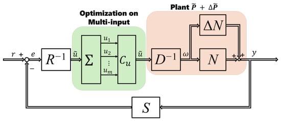
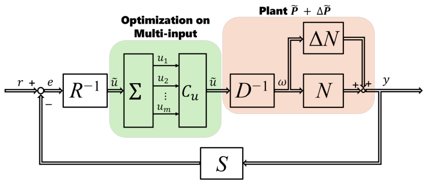
Given the decoupling approach in Figure 3b, an operator-based optimized RRCF feedback system is designed as in Figure 4.

Figure 4. Operator-based optimized RRCF feedback system design.

Specifically, $y\left(t\right)=(P+\Delta P)\left(u\right)\left(t\right)$ denotes the actual overall plant and the nominal plant is divided into $\tilde{P}:\{P_{y1},\dots ,P_{yn}\}$. The outputs are denoted as $\mathit{y}\left(t\right):\{y_1,\dots ,y_n\}$ and the input to each individual plant is $\tilde{u}\left(t\right):\{{\tilde{u}}_1,\dots ,{\tilde{u}}_n\}$. $\Delta \tilde{P}$ denotes the unknown but bounded perturbations. As a result, the plant to be controlled is written as $\mathit{y}\left(t\right)=(\tilde{P}+\Delta \tilde{P})\left(\tilde{u}\right)\left(t\right)$. $\mathit{N},D,S,$ and R are deigned to satisfy the nominal Bezout Identity (1), by which the RCF of $\tilde{P}$ is conducted.

In addition, let $C_u:U\to \tilde{U}$ denote the coupling mapping from the original multi-input vector $u=(u_1,u_2,\dots ,u_m)$ to the reduced input $\tilde{u}$, where $\tilde{U}$ is the linear space of $\tilde{u}:[0,\infty )\to {\mathbb{R}}^n$. For a given $\tilde{u}\in \tilde{U}$, define the feasible set

$$\mathcal{C}\left(\tilde{u}\right)=\left\{u\in U:C_u\left(u\right)=\tilde{u}\right\}.$$

(5)

Since $C_u$ is generally not injective, more than one input vector may belong to $\mathcal{C}\left(\tilde{u}\right)$. The optimized input-allocation mapping

$$\Sigma :\tilde{U}\to U$$

is therefore introduced as a selection mapping that chooses, from $\mathcal{C}\left(\tilde{u}\right)$, an admissible input vector minimizing the quadratic control-effort objective

$$J(u_1,u_2,\dots ,u_m)=u_1^2+u_2^2+\cdots +u_m^2.$$

(6)

More specifically, it can be formulated as

$$\Sigma \left(\tilde{u}\right)\in \underset{u\in \mathcal{C}\left(\tilde{u}\right)}{\arg \min }J\left(u\right).$$

(7)

It is assumed that the feasible set is nonempty and that a minimizer exists for each admissible $\tilde{u}$. By construction, $\Sigma \left(\tilde{u}\right)\in \mathcal{C}\left(\tilde{u}\right)$, and hence

$$C_u\left(\Sigma \left(\tilde{u}\right)\right)=\tilde{u}.$$

(8)

Therefore, $\Sigma$ acts as a right inverse of $C_u$ on the considered admissible set; i.e., $C_u\Sigma =I$, where I denotes the identity operator on $\tilde{U}$.

Theorem 1. 

Consider the operator-based optimized RRCF system shown in Figure 4. Suppose that the operators N, D, S, and R satisfy the nominal Bezout Identity $SN+RD=M$, where M is unimodular. If the allocation mapping $\Sigma :\tilde{U}\to U$ satisfies (8), then the introduction of the optimized multi-input allocation preserves the BIBO stability of the nominal RRCF feedback system.

Proof. 

Since the coupling mapping $C_u$ is generally not injective, the inverse mapping from a given reduced input $\tilde{u}\in \tilde{U}$ to the original multi-input vector $u\in U$ is not necessarily unique. The role of $\Sigma$ is to select one admissible input vector from the feasible set $\mathcal{C}\left(\tilde{u}\right)$ according to the quadratic control-effort criterion in (6). By the definition of the feasible allocation,

$$C_u\left(\Sigma \left(\tilde{u}\right)\right)=\tilde{u},\forall \tilde{u}\in \tilde{U},$$

and therefore

$$C_u\Sigma =I.$$

(9)

Equation (9) implies that, under the ideal allocation condition, the cascade of the allocation mapping $\Sigma$ and the coupling mapping $C_u$ leaves the reduced input $\tilde{u}$ unchanged. Consequently, the effective input–output mapping seen by the nominal RRCF feedback system is identical to that used in the original controller design. Hence, the Bezout Identity of the optimized system remains

$$SN+R{(C_u\Sigma )}^{-1}D=SN+RD=M.$$

(10)

Since M is unimodular, i.e., since both M and $M^{-1}$ are stable operators, Lemma 1 guarantees that the resulting feedback system is BIBO stable.    □

Note that the analysis above focuses on the nonlinear scenarios, which can be viewed as an extension of the linear case, where such inverse mapping is generally interpreted as the Moore—Penrose pseudo-inverse. Moreover, the RRCF feedback system is initially constructed based on the nominal Bezout Identity; i.e., the controllers $\mathit{S}$ and $\mathit{R}$ are designed for $\tilde{P}$. The optimization of multiple inputs is then implemented on $\tilde{u}$, which selects the ideal proper inputs from $\mathcal{C}\left(\tilde{u}\right)$. This process indicates the practical feasibility of utilizing $\Sigma$, since the domain and range of ${\mathit{C}}_u(\Sigma \left(\tilde{u}\right))$ are determined. Under this ideal condition, all couplings present in the system can be represented by ${\mathit{C}}_u$ and eliminated through the optimization. However, in practice, the exact coupling model is often unavailable, and the optimization algorithm may not converge to the optimal solution. As a result, (9) may not hold, and the validity of (10) thus cannot be guaranteed. Therefore, a robustness analysis of the proposed method in general case is provided in the following.

Theorem 2. 

Let ${\Xi }^e$ be a linear subspace of the extended linear space $\mathit{U}$ associated with the Banach space ${\mathit{U}}_B$. Let ${\Xi }^e$ be a stable subspace of $\mathit{U}$.

Consider an operator-based optimized RRCF system as in Figure 4, where $\mathit{N},D,S,$ and R satisfy the nominal Bezout Identity (1). Let ${\tilde{D}}^{-1}:\tilde{U}\to W$ denote the mapping of ${\mathit{D}}^{-1}{C}_u\Sigma \left(\tilde{u}\right)$, where Σ satisfies (7). Then the system in Figure 4 is stable if

$$\parallel [SN-S(N+\Delta N)+RD-R\tilde{D}]M^{-1}{\parallel }_{\mathcal{L}}<1$$

(11)

holds for any $\mathit{r}\in {\Xi }^e$.

Proof. 

Similarly, verifying the stability of the proposed optimized RRCF feedback system amounts to checking whether the Bezout Identity holds with aforementioned errors. Given the definition that ${\tilde{D}}^{-1}\left(\tilde{u}\right)=D^{-1}{C}_u\Sigma \left(\tilde{u}\right)$, the errors arising from unclear coupling and optimization computation can be interpreted as perturbations entering ${\mathit{D}}^{-1}$. In this sense, the current Bezout Identity is written as

$$S(N+\Delta N)+R\tilde{D}=M_{op}$$

(12)

To investigate ${\mathit{M}}_{op}$, the nominal Bezout Identity is introduced to (12), which results in

$$\begin{array}{cc}\hfill M_{op}& =M-SN+S(N+\Delta N)-RD+R\tilde{D}\hfill \\ \hfill & =M-(SN-S(N+\Delta N)+RD-R\tilde{D})\hfill \\ \hfill & =[I-(SN-S(N+\Delta N)+RD-R\tilde{D})M^{-1}]M\hfill \end{array}$$

where $(SN-S(N+\Delta N)+RD-R\tilde{D})M^{-1}:\mathit{U}\to U$ is a stable mapping provided that (11) is satisfied. Hence, ${\mathit{M}}_{op}:W\to U$ is stable since $\mathit{I}$ and $\mathit{M}$ are stable. Next, inverse mapping ${\mathit{M}}_{op}^{-1}$ is formulated as

$$M_{op}^{-1}=M^{-1}{[I-(SN-S(N+\Delta N)+RD-R\tilde{D})M^{-1}]}^{-1}$$

where ${\mathit{M}}^{-1}$ is obviously stable because of the unimodular property. Moreover, ${[I-(SN-S(N+\Delta N)+RD-R\tilde{D})M^{-1}]}^{-1}:U\to U$ is confirmed to exist and is stable given the condition (11) and the property of generalized Lipschitz operator introduced in [11]. Therefore, the mapping ${\mathit{M}}_{op}^{-1}:U\to W$ is proved to be stable and unimodular, by which the Bezout Identity in (12) holds and robust stability of the proposed optimized RRCF feedback system is derived.    □

Up to this point, the stability of the proposed optimized RRCF feedback system design has been analyzed for both the ideal case and the general case, and the results establish robust BIBO stability. According to the proposed optimized framework, the complexity of control design is reduced based on lower-dimensional representation of the outputs, and the optimized multi-input allocation is achieved using feedforward allocation ($\Sigma$) subject to coupling, while the feedback loop is primarily used for robust BIBO stability. It should be noted that, when the coupling model is inaccurate, couplings among the reduced inputs/outputs may still remain after the decoupling procedure shown in Figure 3b. Although, according to Theorem 2, such couplings do not affect the system stability as long as the condition in (11) is satisfied, the further elimination of these couplings remains an important topic for future work. The optimization algorithm for (5) and (7) is expected to be designed in accordance with particular cases. For the following section, the proposed framework as shown in Figure 4 will be applied into a vibrating plate system, by which the aforementioned superiority can be verified.

4. Application to a Vibrating Plate System

4.1. Experimental Set Up

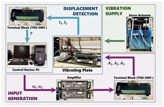
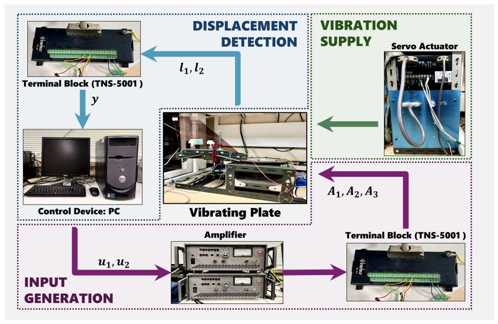
In this section, the proposed control framework is applied to a vibrating flat-plate system. Initially, the experimental set up is exhibited in Figure 5, which mainly includes a PC for input-signal generation, two amplifiers (NF Corporation, Yokohama, Japan, HSA4051; DC–500 kHz) for signal processing, a servo motor actuator (Yokogawa Electric Corporation, Tokyo, Japan, SDB1030-1) for vibration supply and a vibrating plate to be controlled.

Figure 5. Experimental process and devices.

The experimental process can be concluded as follows. Initially, the DC gain is adjusted by servo actuator to generate vibration of servo motor, which in turn induces vibration of the vibrating plate. Next, vibration of the plate is measured by piezoelectric sensors ${\mathit{l}}_1$ and ${\mathit{l}}_2$ of each group mounted on the plate, and the data $\mathit{y}$ is acquired via a terminal block. Then, given current vibration and through computational implementation of the program, desired control inputs ${\mathit{u}}_1$ and ${\mathit{u}}_2$ are obtained and sent to amplifiers, from which the processed input will drive the piezoelectric actuators ${\mathit{A}}_1$, ${\mathit{A}}_2$ and ${\mathit{A}}_3$ of each group to perform vibration control.

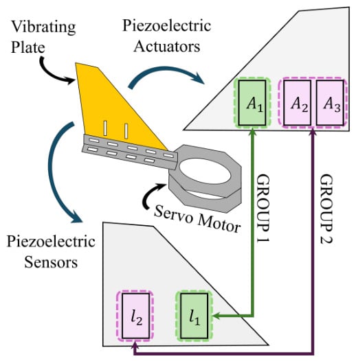
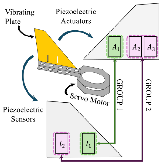
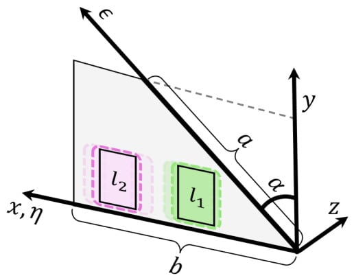
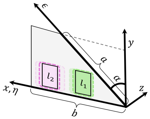
In addition, Figure 6 and Figure 7 show the structural details of the vibrating plate system. As in Figure 6, 3 piezoelectric actuators are attached on the one side, while 2 piezoelectric sensors are mounted on another side. The vibrating plate is described in the $\mathit{xyz}$ coordinates illustrated in Figure 7, where $\mathit{a}$ and $\mathit{b}$ denotes the length in $\eta$ and $ϵ$ direction, respectively, and $\alpha$ denotes the angle between the plate and $\mathit{y}$-axis. Side $\eta$ is clamped, while the remaining three sides are free to vibrate.

Figure 6. The structure of the vibrating plate.

Figure 7. The coordinates of the vibrating plate.

In the previous study [23], the optimal positions of piezoelectric devices have been selected by an iterative algorithm using finite element method on ANSYS 17.0. Moreover, according to the finite-element analysis reported in [23], actuators ${\mathit{A}}_2$ and ${\mathit{A}}_3$ are treated as one group, and are driven by the same input voltage, as illustrated in Figure 6, in order to generate a larger control torque at the corresponding locations.

However, according to the concept introduced in Section 3, the two sets of actuators, ${\mathit{A}}_1$ and ${\mathit{A}}_{2,3}$, act as two inputs for one target, which is different from [26,27]. Therefore, in this paper, only the output of sensor ${\mathit{l}}_2$ will be selected as the feedback signal within the proposed control framework, namely, the optimized RRCF feedback system is designed only focusing on the location of ${\mathit{l}}_2$. In addition, sensor ${\mathit{l}}_1$ is retained for monitoring the control performance driven by ${\mathit{A}}_1$ and ${\mathit{A}}_{2,3}$. Such selection is conducted following the principle of bending energy density [28,29] and is introduced as follows.

Initially, since piezoelectric devices are sensitive to strain (or curvature), the bending energy density [28,29] is used here to describe the strain distribution at each position. Recall the formulation of ${\omega }_d(ϵ,\eta ,t)$ [23] as follows

$${\omega }_d(ϵ,\eta ,t)={\displaystyle \sum _{\xi =1}^{\infty }}{\displaystyle \sum _{\zeta =1}^{\infty }}{\varphi }_{\xi }\left(ϵ\right){\psi }_{\zeta }\left(\eta \right)·f\left(t\right),$$

(13)

which denotes the transverse displacement field of the plate at the spatial coordinate $(ϵ,\eta )$ and time t. ${\varphi }_{\xi }\left(ϵ\right)$ and ${\psi }_{\zeta }\left(\eta \right)$ denotes the instinct functions of $ϵ$ and $\eta$ direction, as shown in Figure 7. $\mathit{f}\left(t\right)$ in (13) is the displacement in a mode coordinate system of the vibrating plate, which is further explained in Appendix A. Specifically, details of ${\varphi }_{\xi }\left(ϵ\right)$ and ${\psi }_{\zeta }\left(\eta \right)$ are presented as follows.

$$\begin{array}{cc}\hfill {\varphi }_1\left(ϵ\right)& =\cosh \left({\displaystyle \frac{{\gamma }_{ϵ,1}}{a}}ϵ\right)-\cos \left({\displaystyle \frac{{\gamma }_{ϵ,1}}{a}}ϵ\right)-c_1\left[\sinh \left({\displaystyle \frac{{\gamma }_{ϵ,1}}{a}}ϵ\right)-\sin \left({\displaystyle \frac{{\gamma }_{ϵ,1}}{a}}ϵ\right)\right]\hfill \\ \hfill {\varphi }_{\xi }\left(ϵ\right)& =\cosh \left({\displaystyle \frac{{\gamma }_{ϵ,\xi }}{a}}ϵ\right)-\cos \left({\displaystyle \frac{{\gamma }_{ϵ,\xi }}{a}}ϵ\right)-\sinh \left({\displaystyle \frac{{\gamma }_{ϵ,\xi }}{a}}ϵ\right)+\sin \left({\displaystyle \frac{{\gamma }_{ϵ,\xi }}{a}}ϵ\right),(\xi >1)\hfill \\ \hfill {\psi }_1\left(\eta \right)& =1\hfill \\ \hfill {\psi }_2\left(\eta \right)& =\sqrt{3}\left(1-{\displaystyle \frac{2\eta }{b}}\right)\hfill \\ \hfill {\psi }_{\zeta }\left(\eta \right)& =\cosh \left({\displaystyle \frac{{\gamma }_{\eta ,\zeta }}{b}}\eta \right)+\cos \left({\displaystyle \frac{{\gamma }_{\eta ,\zeta }}{b}}\eta \right)-\sinh \left({\displaystyle \frac{{\gamma }_{\eta ,\zeta }}{b}}\eta \right)-\sin \left({\displaystyle \frac{{\gamma }_{\eta ,\zeta }}{b}}\eta \right),(\zeta >2)\hfill \end{array}$$

where ${\gamma }_{ϵ,\xi }={\displaystyle \frac{(2\xi -1)\pi }{2}}$ and ${\gamma }_{\eta ,\zeta }={\displaystyle \frac{(2\zeta -3)\pi }{2}}$. The coefficient $c_1$ is associated with the first-mode spatial function under the corresponding plate boundary condition. Following the classical modal formulation reported in [30] and the approximation adopted in the previous work [23], $c_1=0.7$ is used in the present study. Then, based on the transverse displacement ${\omega }_d$ in (13), the bending curvatures along the $ϵ$- and $\eta$-directions and the twisting curvature of the plate are obtained as

$${\kappa }_{ϵ}={\displaystyle \frac{{\partial }^2{\omega }_d}{\partial {ϵ}^2}},{\kappa }_{\eta }={\displaystyle \frac{{\partial }^2{\omega }_d}{\partial {\eta }^2}},{\kappa }_{ϵ\eta }=2{\displaystyle \frac{{\partial }^2{\omega }_d}{\partial ϵ\partial \eta }}$$

which results in the bending energy density being

$$u_b(ϵ,\eta )={\displaystyle \frac{1}{2}}{\mathit{D}}_b\left({\kappa }_{ϵ}^2+{\kappa }_{\eta }^2+2\nu {\kappa }_{ϵ}{\kappa }_{\eta }+{\displaystyle \frac{1-\nu }{2}}{\kappa }_{ϵ\eta }^2\right)$$

where $\nu$ denotes the Poisson’s ratio, ${\mathit{D}}_b=E{h}^3/12(1-{\nu }^2)$, $\mathit{E}$ is the Young’s modulus and $\mathit{h}$ is the thickness of vibrating plate.

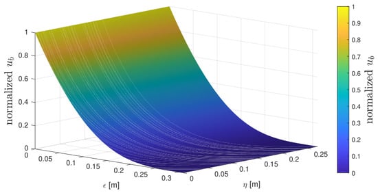
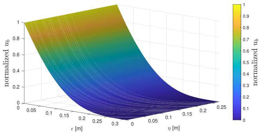
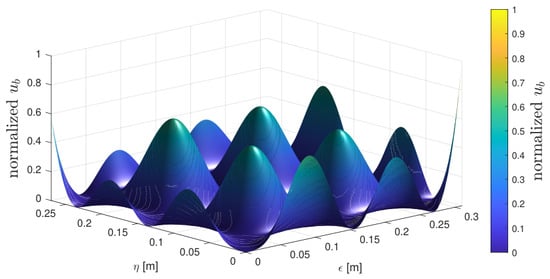
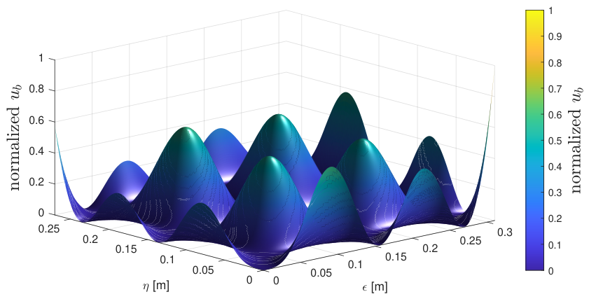
The visible analysis of normalized bending energy density in different modes is exhibited in Figure 8 and Figure 9. Generally, the first mode ($\xi =\zeta =1$) of the plate is excited in the experiment, corresponding to the vibration frequency of the servo motor. Then according to the results in Figure 8, one can find the maximum bending energy near the $\eta$-axis, which is clamped. This explains the necessity of placing the piezoelectric devices near the $\eta$-axis as [23,27]. Moreover, higher-order modes of the plate vibration are likely to be excited due to the loosening clamp caused by long-term operation. Hence, the analysis on the third mode ($\xi =\zeta =3$) is conducted as in Figure 9, where the higher bending energy can be observed around $\eta =0.2$ m and $ϵ=0.05$ m, which contributes to the selection of sensor ${\mathit{l}}_2$ as the objective control target.

Figure 8. Distribution of bending energy density ${\mathit{u}}_b$ when $\xi =\zeta =1$.

Figure 9. Distribution of bending energy density ${\mathit{u}}_b$ when $\xi =\zeta =3$.

In addition, the decision about sensor ${\mathit{l}}_2$ can be further substantiated through the following mathematical analysis. Write the relations from inputs to outputs of the MIMO vibrating plate system as

$$\left[\begin{array}{c}{y}_1\\ y_2\end{array}\right]=\underset{\mathcal{A}}{\underbrace{\left[\begin{array}{cc}{a}_{11}& a_{12}\\ a_{21}& a_{22}\end{array}\right]}}\left[\begin{array}{c}{u}_1\\ u_2\end{array}\right]$$

where ${\mathit{y}}_1$ and $y_2$ denote the outputs detected by sensors ${\mathit{l}}_1$ and ${\mathit{l}}_2$, ${\mathit{u}}_1$ and $u_2$ are the inputs toward actuators ${\mathit{A}}_1$ and ${\mathit{A}}_{2,3}$. ${\mathit{a}}_{11}$ and ${\mathit{a}}_{22}$ denote the individual mappings of each group, while ${\mathit{a}}_{12}$ and ${\mathit{a}}_{21}$ serve as the couplings. Given the structural analysis above and the experimental statistics from previous research [26], ${\mathit{y}}_1$, i.e., the results detected by sensor ${\mathit{l}}_1$, is slight compared to ${\mathit{y}}_2$, which suggests a slighter scale (${10}^{-1}$) of mappings ${\mathit{a}}_{11}$ and ${\mathit{a}}_{12}$. Therefore, the inverse mapping ${\mathcal{A}}^{-1}$ may be ill-conditioned in this sense, so that the direct inference of coupling from ${\mathit{y}}_1$ and ${\mathit{y}}_2$ to ${\mathit{u}}_1$ and ${\mathit{u}}_2$ becomes unreliable. As a result, the induced numerical errors are unacceptable for accurately characterizing the coupling from the output to multiple inputs. In contrast, it is more appropriate to explicitly consider the coupling among the inputs and optimize it directly. Accordingly, the coupling from ${\mathit{u}}_1$ to ${\mathit{u}}_2$, which is equivalent in effect to ${\mathit{a}}_{21}$, is considered, and the nonlinear RRCF feedback system will be established based on the dynamics detected by sensor ${\mathit{l}}_2$ in the following sections.

4.2. Specific Control System for Vibrating Plate

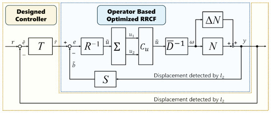
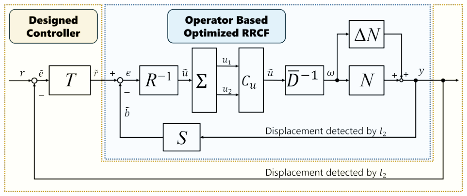
Rewrite the vibrating model on the location of ${\mathit{l}}_2$ as $\tilde{P}$, the specific control system for vibrating plate can be depicted as in Figure 10.

Figure 10. Operator-based optimized RRCF feedback system design for a vibrating plate, where the displacement is detected by sensor ${\mathit{l}}_2$.

To begin with, without consideration of hysteresis and perturbations, the mathematical dynamics of vibrating plate are formulated as

$$y(ϵ,\eta ,t)={\displaystyle \sum _{\xi =1}^{\infty }}{\displaystyle \sum _{\zeta =1}^{\infty }}\left({\int }_0^t{J}_{\xi \zeta }{e}^{-{\alpha }_{\xi \zeta }(t-\tau )}·\sin {\beta }_{\xi \zeta }(t-\tau )·{\tilde{M}}_p\left(\tau \right)d\tau \right).$$

(14)

In this work, the first mode of (14) is selected so as to denote the nominal plant, while the second and third modes are considered as perturbations. As a result, the plant $\tilde{P}+\Delta \tilde{P}$ can be formulated as

$$\begin{array}{cc}\hfill y\left(t\right)& =\tilde{P}+\Delta \tilde{P}\left(\tilde{u}\right)\hfill \\ \hfill & =(1+\Delta )\left[{\int }_0^t{J}_{11}{e}^{-{\alpha }_{11}(t-\tau )}·\sin {\beta }_{11}(t-\tau )·\tilde{u}\left(\tau \right)d\tau \right]\hfill \end{array},$$

(15)

where $\tilde{u}$ denotes the total driving voltage required at the location of sensor ${\mathit{l}}_2$, $\Delta$ denotes the simplified second and third modes. This total voltage corresponds to the resultant control torque required at that location. In the experiment, however, this total voltage is not physically applied to a single actuator. Instead, it is allocated to the two actuator groups through the optimization procedure. The detailed derivation of (14) and (15) is found in Appendix A. Then the plant $\tilde{P}+\Delta \tilde{P}$ is factorized into $\mathit{N}+\Delta N$ and ${\mathit{D}}^{-1}$ as

$$\begin{array}{cc}\hfill & (\mathit{N}+\Delta N)\left(\omega \right):y\left(t\right)=(1+\Delta )\left[J_{11}{\int }_0^t{e}^{-{\alpha }_{11}(t-\tau )}·\sin {\beta }_{11}(t-\tau )·\omega \left(\tau \right)d\tau \right]\hfill \\ \hfill & D\left(\omega \right):\tilde{u}\left(t\right)=I\left(\omega \right)\left(t\right)\hfill \end{array}$$

Next, consider the hysteresis component of piezoelectric actuators. According to the results included in [10,23], the input hysteresis model of piezoelectric actuators can be formulated as $\mathcal{H}\left(\tilde{u}\right)=(D_{PI}+d)\left(\tilde{u}\right)$, where ${\mathit{D}}_{PI}$ is interpreted as a linear operator and denoted as ${\mathit{D}}_{PI}=\mathit{K}={\int }_0^{H}p\left(h\right)dh$, while $\mathit{d}(·)$ is a nonlinear residual. Then operator $\overline{D}$ is defined as $\overline{D}={\mathit{D}}_{PI}^{-1}D$ for further nominal controller design. However, since the vibrating plate is performing relatively small displacement around 0, the nonlinear part $\mathit{d}$ is treated as slight bounded external disturbance [10,23], which is a part of $\Delta N$ and is ignored for nominal operator design in this work.

Then, controllers $\mathit{S}$ and $\mathit{R}$ are designed as

$$\begin{array}{cc}\hfill & S\left(y\right):b\left(t\right)=\left({\displaystyle \frac{1-K_m}{J_{11}{\beta }_{11}}}\right)\left(\ddot{y}\left(t\right)+2{\alpha }_{11}\dot{y}\left(t\right)+\left({\alpha }_{11}^2+{\beta }_{11}^2\right)y\left(t\right)\right)\hfill \\ \hfill & R\left(\tilde{u}\right):e\left(t\right)=K_m{D}_{PI}\left(\tilde{u}\right)\left(t\right)\hfill \end{array}$$

where ${\mathit{K}}_m$ is a designed parameter. As result, it can be found that the Bezout Identity

$$SN\left(\omega \right)+R\tilde{D}\left(\omega \right)=I\left(\omega \right)$$

is satisfied, which indicates that the robust stability of the proposed control system is guaranteed.

Next, we focus on the optimization $\Sigma$ and coupling ${\mathit{C}}_u$. In previous research [26], the effect from actuator ${\mathit{P}}_1$ working on ${\mathit{l}}_2$ has been formulated as

$$G\left(u_1\right)\left(t\right)=-{\alpha }_1{u}_1^2\left(t\right)\mathrm{sign}\left(u_1\left(t\right)\right)+{\alpha }_2{u}_1\left(t\right),$$

where ${\alpha }_1=-1.20445\times {10}^{-3}$ and ${\alpha }_2=0.681111$. This results in the formulation of ${\mathit{C}}_u$ as

$$\begin{array}{cc}\hfill \tilde{u}& =C_u(u_1,u_2)=u_2+G\left(u_1\right)\hfill \\ \hfill & =u_2-{\alpha }_1{u}_1^2\left(t\right)\mathrm{sign}\left(u_1\left(t\right)\right)+{\alpha }_2{u}_1\left(t\right).\hfill \end{array}$$

To explicitly account for the actuator voltage limits in the practical experiments, the multi-input allocation problem $\Sigma$ is reformulated as

$$\begin{array}{cc}\hfill (u_1^{\ast },u_2^{\ast })& \in \arg \underset{u_1,u_2}{\min }{u}_1^2+u_2^2\hfill \\ \hfill \mathrm{subject}\mathrm{to}& \tilde{u}=u_2-{\alpha }_1{u}_1^2\mathrm{sign}\left(u_1\right)+{\alpha }_2{u}_1,\hfill \\ \hfill & |u_1|\le u_{\max },\left|u_2\right|\le u_{\max },\hfill \end{array}$$

where $u_{\max }=100$ denotes the maximum admissible voltage.

By eliminating $u_2$ from the equality constraint, one obtains

$$u_2\left(u_1\right)=\tilde{u}+{\alpha }_1{u}_1^2\mathrm{sign}\left(u_1\right)-{\alpha }_2{u}_1.$$

(16)

Accordingly, the constrained two-variable optimization is reduced to the scalar problem

$$\underset{u_1\in \mathbb{R}}{\min }f\left(u_1\right)\mathrm{subject}\mathrm{to}|u_1|\le u_{\max },\left|u_2\left(u_1\right)\right|\le u_{\max }$$

with

$$f\left(u_1\right)=u_1^2+{\left(\tilde{u}+{\alpha }_1{u}_1^2\mathrm{sign}\left(u_1\right)-{\alpha }_2{u}_1\right)}^2$$

(17)

Since $\mathrm{sign}\left(u_1\right)$ is piecewise-defined, the stationary conditions are derived separately for the cases $u_1>0$ and $u_1<0$. For $u_1>0$, define

$$f_{+}\left(u_1\right)=u_1^2+{\left(\tilde{u}+{\alpha }_1{u}_1^2-{\alpha }_2{u}_1\right)}^2,$$

whose stationary points satisfy

$$2{\alpha }_1^2{u}_1^3-3{\alpha }_1{\alpha }_2{u}_1^2+(2{\alpha }_1\tilde{u}+{\alpha }_2^2+1)u_1-{\alpha }_2\tilde{u}=0.$$

(18)

For $u_1<0$, define

$$f_{-}\left(u_1\right)=u_1^2+{\left(\tilde{u}-{\alpha }_1{u}_1^2-{\alpha }_2{u}_1\right)}^2,$$

whose stationary points satisfy

$$2{\alpha }_1^2{u}_1^3+3{\alpha }_1{\alpha }_2{u}_1^2+(1-2{\alpha }_1\tilde{u}+{\alpha }_2^2)u_1-{\alpha }_2\tilde{u}=0.$$

(19)

In addition to the interior stationary points and the seam point $u_1=0$, boundary candidates associated with $u_1=\pm u_{\max }$ and $u_2=\pm u_{\max }$ are also examined. The complete solution procedure is summarized in Algorithm 1. For the experimental conditions considered in this paper, the admissible range of $\tilde{u}$ ensures that the feasible candidate set is always nonempty. Algorithm 1 is not an iterative optimization routine, but a finite candidate selection procedure. After constraint elimination, the solution is determined by solving fixed-degree polynomial equations and evaluating a finite set of feasible candidates, including both interior stationary points and boundary points associated with the input limits. Hence, the algorithm is guaranteed to terminate in a finite number of operations. In addition, because both the problem dimension and the polynomial degrees are fixed, the per-step computational complexity is $O\left(1\right)$.

Algorithm 1: Constrained minimum-control-effort input allocation for the vibrating plate system

Input: $\tilde{u}$, ${\alpha }_1$, ${\alpha }_2$, and $u_{\max }$.   Output: An optimal input pair $(u_1^{\ast },u_2^{\ast })$.   Eliminate $u_2$ using (16) and construct the scalar objective $f\left(u_1\right)$ in (17).   Derive the stationary-point equations for the cases $u_1>0$ and $u_1<0$, given by (18) and (19), respectively.   Compute all real stationary candidates together with the seam point $u_1=0$.   Construct boundary candidates associated with $u_1=\pm u_{\max }$ and $u_2=\pm u_{\max }$.   Discard all infeasible candidates violating $|u_1|\le u_{\max }$ or $|u_2|\le u_{\max }$.   Evaluate $f\left(u_1\right)$ for all feasible candidates and select the $u_1^{\ast }$ satisfying the minimum.      Recover $u_2^{\ast }$ from (16).   return $(u_1^{\ast },u_2^{\ast })$

Moreover, to improve the tracking performance for vibration suppression, an additional controller $\mathit{T}$ is introduced as

$$T:\tilde{r}\left(t\right)=-K_p\tilde{e}\left(t\right)-K_c{Q}^{-\varrho }\left(t\right)\dot{\tilde{e}}\left(t\right),$$

(20)

where $\tilde{e}\left(t\right)=r\left(t\right)-y\left(t\right)$, and ${\mathit{K}}_p>0$, ${\mathit{K}}_c>0$, and $\varrho \in (0,0.5)$ are design parameters. While (20) is reminiscent of a proportional-derivative control law, the derivative gain is made adaptive to better handle high-frequency vibration modes. To this end, define

$$Q\left(t\right)={\epsilon }_{\mathcal{Q}}+{\displaystyle \frac{{\dot{y}}^2\left(t\right)}{2}}+{\displaystyle \frac{K_p{y}^2\left(t\right)}{2}}.$$

Here, $Q\left(t\right)$ acts as an energy-like measure of the instantaneous vibration level. Hence, the factor $Q^{-\varrho }\left(t\right)$ adaptively modulates the derivative action: when the vibration level is large, $Q\left(t\right)$ increases and the effective derivative gain decreases, which suppresses excessive sensitivity to high-frequency oscillations; when the vibration level becomes small, $Q\left(t\right)$ decreases and the derivative action is strengthened, thereby improving tracking precision. In addition, the constant ${\epsilon }_{\mathcal{Q}}$ is introduced to guarantee $Q\left(t\right)>0$, so that the term $Q^{-\varrho }\left(t\right)$ remains well-defined and bounded. As a result, the robust stability of the proposed scheme is guaranteed by operator-based optimized right coprime factorization, and the designed controller contributes to better tracking performance. For the next step, practical experiments based on the proposed design are conducted.

4.3. Experimental Results

The results of practical experiments are exhibited. The experiment was conducted with a sampling period of 1 ms and the signal conversion was implemented with a 12-bit resolution. A total of 10,000 samples were collected, corresponding to a duration of 10 s, and the control is applied from the 3000th sampling instant, namely, $\mathit{t}$ = 3 s. To evaluate the control performance on vibrating plate, the following criteria are introduced. Specifically, $\mathit{S}$ is defined as the suppression rate, which is denoted as

$$S_{avg}=(1-{\displaystyle \frac{{\sigma }_c}{{\sigma }_o}})\times 100\%$$

where ${\sigma }_o$ denotes the distribution of displacement without implementing control strategies, and ${\sigma }_c$ denotes the one under control. ${\sigma }_o$ and ${\sigma }_c$ are formulated as

$${\sigma }_o={\displaystyle \frac{{\int }_{T_0}^{T_s}\left|y\left(t\right)\right|dt}{T_s-T_0}},{\sigma }_c={\displaystyle \frac{{\int }_{T_s}^T\left|y\left(t\right)\right|dt}{T-T_s}}$$

where ${\mathit{T}}_0$, ${\mathit{T}}_s$ and $\mathit{T}$ denote the initial time, control starting time and stopping time. As stated earlier, although the system design only uses the dynamics at sensor ${\mathit{l}}_2$, sensor ${\mathit{l}}_1$ is retained to validate the effectiveness of the proposed control framework. Accordingly, ${\mathit{S}}_{avg}^{l_i}$, ${\sigma }_o^i$ and ${\sigma }_c^i$ are introduced to denote the evaluations at ${\mathit{l}}_i$, $\mathit{i}=1,2$.

Analogously, $V_{avg}^{A_j}$ is defined as

$$V_{avg}^{A_j}={\displaystyle \frac{{\int }_{T_s}^T{u}_j{\left(t\right)}^{2}dt}{T-T_s}}$$

which aims to analyze the consumption of voltage-based control effort. Note that $\mathit{j}=1,2,3$ and ${\mathit{u}}_3={\mathit{u}}_2$ since ${\mathit{A}}_2$ and ${\mathit{A}}_3$ are of the same group. Hence, the total control effort is derived as

$$V_{avg}^s=V_{avg}^{A_1}+2V_{avg}^{A_2}$$

and the ratio of each actuator is defined as

$${\Gamma }_j={\displaystyle \frac{V_{avg}^{A_j}}{V_{avg}^s}}\times 100\%$$

by which the multi-input allocation is quantified.

Comparative experiments are carried out among the following control schemes: (1) sliding mode control (SMC), (2) ${\mathit{H}}_{\infty }$ control, (3) linear quadratic regulation (LQR), (4) the previous operator-based method in [27], and (5) the proposed method. In all cases, the coupling among multiple inputs is explicitly taken into consideration. For each control scheme, the controller parameters are determined through repeated tuning under the same vibration mode. In particular, the parameter setting of the proposed method is specified as follows: ${\mathit{K}}_p=10.0$, ${\mathit{K}}_{\mathit{c}}=0.095$, $\varrho =0.45$ and ${\epsilon }_{\mathcal{Q}}=1\times {10}^{-6}$. Other parameters for experiments are listed in Table 1.

Table 1. Parameters of model.

Parameter	Value	Parameter	Value
${\mathit{J}}_{11}$	0.1073	${\mathit{K}}_m$	0.2
${\alpha }_{11}$	0.1049	${\beta }_{11}$	32.7406

In the experiments, the servo actuator parameters are first fixed so that the driving command remains unchanged over the entire test interval. This case is termed the constant-mode. Then, to demonstrate the robustness of the proposed scheme against variations in the actuator dynamics, the parameter ${\mathit{f}}_c$ of the servo actuator is randomly perturbed during $\mathit{t}\in [3\mathrm{s},7\mathrm{s}]$ (switching ${\mathit{f}}_c$ between two selected frequency), with all the remaining parameters unchanged. Here, ${\mathit{f}}_c$ represents the natural frequency, i.e., the positioning bandwidth, of the servo system. Each perturbed value is held for a randomly selected duration shorter than 1 s. This case is termed the varying-mode. Ten experimental trials are conducted for each method under each mode.

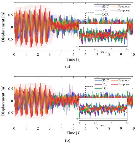
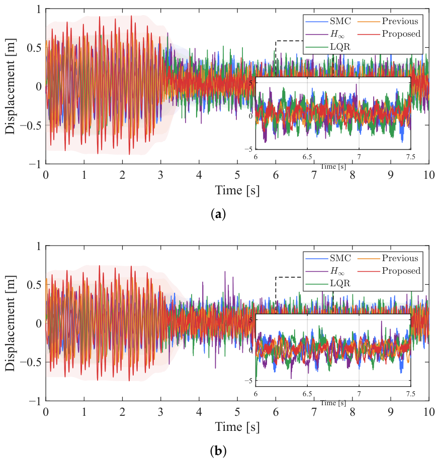
The visible results of constant-mode experiments are exhibited in Figure 11 and Figure 12. Figure 11a and Figure 11b show the vibration detected by sensor ${\mathit{l}}_1$ and ${\mathit{l}}_2$, respectively. It can be observed that the output detected by sensor ${\mathit{l}}_2$ under free vibration is about ten times higher than that of ${\mathit{l}}_1$, confirming the consistency with the structural analysis presented above. Specifically, Figure 11 presents a representative comparison, selected such that the suppression rate of each method is closest to its average value. As can be seen, although identical servo-actuator parameters are used for all methods, namely, the same driving commands are applied to the servo motor, the resulting displacement still exhibits slight trial-to-trial variations due to friction in the servo motor and different signal acquisition timing caused by differences in program initialization time across trials. Despite this effect, the proposed method still achieves the most pronounced vibration suppression among all methods.

Figure 11. Displacements detected by the sensors under constant-mode vibration using different control strategies: (a) Displacement detected by ${\mathit{l}}_1$; (b) displacement detected by ${\mathit{l}}_2$.

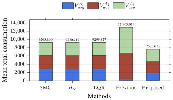
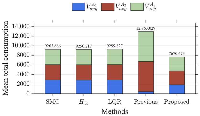
Figure 12. Allocation of multiple inputs under the constant-mode vibration using different control strategies.

The quantitative results are summarized in Table 2. The proposed method achieves average suppression rates of 80.339% and 71.646%, both of which are clearly higher than those obtained by the other methods. In addition, it exhibits the lowest voltage-based control effort and realizes multi-input allocation according to the coupling relationship, as further illustrated in Figure 12. These results demonstrate the effectiveness of the proposed optimized RRCF feedback system design. Moreover, the computational cost of the complete proposed method including Algorithm 1 is 0.536 ms with an interval of [0.504, 0.568] ms. Since this is below the experimental sampling period of 1 ms, the practical feasibility of Algorithm 1 is confirmed.

Table 2. Comparison of different methods under constant-mode vibration. Results are reported as the mean ± half-width of the 95% confidence interval.

Methods	${\mathit{S}}_{\mathbf{avg}}^{{\mathit{l}}_1}$ (%)	${\mathit{S}}_{\mathbf{avg}}^{{\mathit{l}}_2}$ (%)	${\mathit{V}}_{\mathbf{avg}}^{\mathit{s}}$	${\mathbf{\Gamma }}_1$ (%)	${\mathbf{\Gamma }}_2,{\mathbf{\Gamma }}_3$ (%)
SMC	$49.010\pm 2.136$	$39.171\pm 2.243$	$9263.866\pm 58.207$	$30.961\pm 0.105$	$34.519\pm 0.053$
$H_{\infty }$	$51.054\pm 1.808$	$46.954\pm 1.732$	$9250.217\pm 48.764$	$30.709\pm 0.072$	$34.646\pm 0.036$
LQR	$49.967\pm 1.738$	$47.606\pm 1.676$	$9299.827\pm 20.928$	$30.818\pm 0.044$	$34.591\pm 0.022$
Previous method	$72.912\pm 1.482$	$67.676\pm 2.846$	12,963.029 ± 148.036	$3.494\pm 0.139$	$48.253\pm 0.070$
Proposed method	$80.339\pm 0.929$	$71.646\pm 0.874$	$7670.673\pm 107.825$	$24.293\pm 0.066$	$37.853\pm 0.033$

The overall comparison of the online computation time of different control methods is exhibited in Table 3. As shown in Table 3, the conventional SMC, $H_{\infty }$, and LQR controllers require relatively small online computation times, with mean values of $0.0057$, $0.0064$, and $0.0054\mathrm{ms}$, respectively. In comparison, the two operator-based methods require considerably greater computational effort because their online implementations involve additional operator mappings and nonlinear feedback calculations. Nevertheless, the mean computation times of both operator-based methods remain below the experimental sampling period of $1\mathrm{ms}$.

Table 3. Comparison of the online computation time of different control methods.

Method	Mean Computation Time (ms)	Measured Range (ms)
SMC	0.0057	[0.0007, 0.0106]
$H_{\infty }$	0.0064	[0.00047, 0.012]
LQR	0.0054	[0.0005, 0.0102]
Previous method	0.594	[0.564, 0.625]
Proposed method	0.536	[0.504, 0.568]

More importantly, the proposed method requires an average online computation time of $0.536\mathrm{ms}$, compared with $0.594\mathrm{ms}$ for the previous method, corresponding to a reduction of approximately $9.8\%$. This reduction is consistent with the reduced-dimensional control structure of the proposed framework: the feedback controller is constructed using a single reduced input–output control loop rather than separate control loops associated with the higher-dimensional representation. Although the proposed method additionally performs the constrained multi-input allocation during each sampling instant, its total computation time is still lower than that of the previous operator-based method. Therefore, the online allocation procedure does not introduce a dominant computational burden in the present implementation.

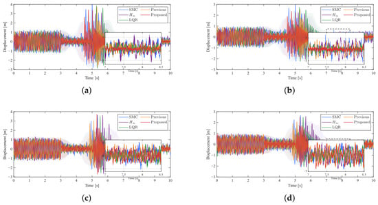
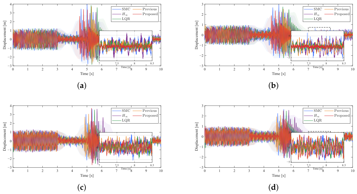
The experimental results under varying-mode vibration are reported in Table 4 and Figure 13. As seen from Table 4, although the experiments are subject to randomly generated perturbations, the proposed method still achieves more significant vibration suppression, with the rates 65.157% and 55.74%, than the other methods. This result supports the robust stability of the proposed method. Moreover, two groups of cases are presented in Figure 13 as representative examples, including one trial whose result is close to the mean and one relatively deviating trial. It can be observed that the system maintains effective vibration suppression even in the presence of perturbations, which further demonstrates the robust stability of the proposed optimized RRCF feedback system.

Table 4. Comparison of different methods under the varying-mode vibration. Results are reported as mean ± half-width of the 95% confidence interval.

Methods	${\mathit{S}}_{\mathbf{avg}}^{{\mathit{l}}_1}$ (%)	${\mathit{S}}_{\mathbf{avg}}^{{\mathit{l}}_2}$ (%)
SMC	44.017 ± 3.866	27.792 ± 4.703
$H_{\infty }$	45.896 ± 2.933	30.372 ± 3.613
LQR	46.467 ± 3.308	32.109 ± 3.210
Previous method	49.631 ± 3.806	39.042 ± 8.178
Proposed method	65.157 ± 4.131	55.740 ± 5.124

Figure 13. Experimental results of two representative cases under varying-mode vibration: (a) Displacement detected by ${\mathit{l}}_1$ in mean-close trial; (b) displacement detected by ${\mathit{l}}_2$ in mean-close trial; (c) displacement detected by ${\mathit{l}}_1$ in mean-deviating trial; (d) displacement detected by ${\mathit{l}}_2$ in mean-deviating trial.

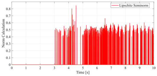
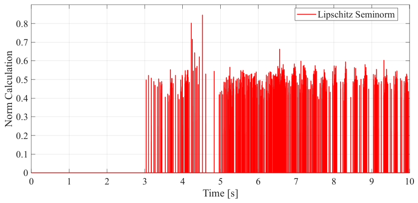
To further examine the robust-stability condition established in Theorem 2, the left-hand side of (11) is numerically evaluated using the experimental data obtained under the varying-mode vibration. A representative trial whose suppression performance is closest to the mean value among all repeated trials is selected for this verification. The resulting generalized Lipschitz calculation is shown in Figure 14. It can be observed that the evaluated value remains below 1 throughout the considered controlled interval. In particular, its maximum value is approximately $0.85<1$. Therefore, the sufficient robust-stability condition in (11) is satisfied for this representative experimental case. This result provides the numerical verification of Theorem 2 in addition to the observed vibration-suppression performance.

Figure 14. Verification of the robust condition (11) using experimental results under varying-mode vibration.

In summary, the proposed control design provides the following advantages. Compared with the previous study [26], the proposed framework provides a concise robust-stability analysis based on the Bezout Identity and optimized multi-input allocation. Since the feedback controller is constructed in a reduced-dimensional input–output space rather than separately according to the full actuator dimension, the controller-design complexity can be reduced. Compared with the case without optimized multi-input allocation, such as [27], the proposed method achieves improved vibration suppression with a lower voltage-based control-effort metric, while distributing the actuator effort more evenly.

In the present implementation, only sensor $l_2$ is required as the feedback signal, whereas sensor $l_1$ is retained only for independent performance monitoring. Therefore, the proposed architecture reduces the number of required feedback sensing channels and the associated signal-processing complexity, which may also reduce the sensing hardware required for implementation. It should nevertheless be emphasized that reducing the feedback dimension may simultaneously discard part of the system information. In the present vibrating-plate experiments, effective vibration suppression is observed at both the feedback sensor $l_2$ and the non-feedback monitoring sensor $l_1$, suggesting that the information reduction does not cause significant performance degradation under the considered experimental conditions. For more general and large-scale systems, however, the minimum level of reduction and decoupling that can be tolerated while retaining sufficient system information remains to be carefully investigated.

5. Conclusions

In this paper, an operator-based optimized RRCF control design is proposed. The proposed framework aims at optimization on multiple-control-input allocation in mechatronic systems. Moreover, the robust stability of this strategy is ensured by the RRCF structure and the interpretation of the optimization process in mapping perspectives. Practical application of the proposed control design on a vibrating plate system is conducted with low-cost device implementation. Compared with current research, the experimental results indicate reduced control design complexity and control effort, enhanced control performance, and balanced workload allocation. All these results demonstrate the effectiveness of the proposed control design.

Although the present experimental implementation employs a finite number of actuator and output channels, the proposed framework is formulated in Banach signal spaces in accordance with the operator-based RRCF theory. This generality may become more advantageous for distributed-parameter systems in which the system variables are naturally function-valued, such as flexible structures described by partial differential equations or systems with spatially distributed sensing and actuation. Extending the proposed optimized multi-input allocation and its robust-stability analysis to such genuinely infinite-dimensional systems constitutes an important direction for future work.

References

- Khalil, H.K.; Grizzle, J.W. Nonlinear Systems, 3rd ed.; Prentice Hall: Upper Saddle River, NJ, USA, 2002. [Google Scholar]
- Isidori, A. Nonlinear Control Systems, 3rd ed.; Springer: London, UK, 1995. [Google Scholar]
- Slotine, J.-J.E.; Li, W. Applied Nonlinear Control; Prentice Hall: Englewood Cliffs, NJ, USA, 1991. [Google Scholar]
- Krstic, M.; Kanellakopoulos, I.; Kokotovic, P.V. Nonlinear and Adaptive Control Design; John Wiley & Sons: New York, NY, USA, 1995. [Google Scholar]
- Spong, M.W. An historical perspective on the control of robotic manipulators. Annu. Rev. Control Robot. Auton. Syst. 2022, 5, 1–31. [Google Scholar] [CrossRef] [Scilit]
- Devasia, S.; Eleftheriou, E.; Moheimani, S.O.R. A survey of control issues in nanopositioning. IEEE Trans. Control Syst. Technol. 2007, 15, 802–823. [Google Scholar] [CrossRef] [Scilit]
- Moheimani, S.O.R.; Fleming, A.J. Piezoelectric Transducers for Vibration Control and Damping; Springer: London, UK, 2006. [Google Scholar]
- Yuan, Z.; Zhou, S.; Zhang, Z.; Xiao, Z.; Hong, C.; Chen, X.; Zeng, L.; Li, X. Piezo-actuated smart mechatronic systems: Nonlinear modeling, identification, and control. Mech. Syst. Signal Process. 2024, 221, 111715. [Google Scholar] [CrossRef] [Scilit]
- Chen, G.; Han, Z. Robust right coprime factorization and robust stabilization of nonlinear feedback control systems. IEEE Trans. Autom. Control 1998, 43, 1505–1509. [Google Scholar] [CrossRef] [Scilit]
- Deng, M. Operator-Based Nonlinear Control Systems: Design and Applications; John Wiley & Sons: Hoboken, NJ, USA, 2014. [Google Scholar]
- De Figueiredo, R.J.P.; Chen, G. Nonlinear Feedback Control Systems: An Operator Theory Approach; Academic Press: San Diego, CA, USA, 1993. [Google Scholar]
- Bu, N.; Chen, W.; Jin, L.; Zhao, Y. Robust control for uncertain nonlinear feedback system using operator-based right coprime factorization. IEEE/CAA J. Autom. Sin. 2019, 6, 824–829. [Google Scholar] [CrossRef] [Scilit]
- Bu, N.; Liu, H.; Li, W. Robust passive tracking control for an uncertain soft actuator using robust right coprime factorization. Int. J. Robust Nonlinear Control 2021, 31, 6810–6825. [Google Scholar] [CrossRef] [Scilit]
- Deng, M.; Bi, S. Operator-based robust nonlinear control system design for MIMO nonlinear plants with unknown coupling effects. Int. J. Control 2010, 83, 1939–1946. [Google Scholar] [CrossRef] [Scilit]
- Wu, Y.; Deng, M. Experimental study on robust nonlinear forced vibration control for an L-shaped arm with reduced control inputs. IEEE/ASME Trans. Mechatron. 2017, 22, 2186–2195. [Google Scholar] [CrossRef]
- Usami, T.; Deng, M. Applying an MSVR method to forecast a three-degree-of-freedom soft actuator for a nonlinear position control system: Simulation and experiments. IEEE Syst. Man Cybern. Mag. 2022, 8, 61–69. [Google Scholar] [CrossRef] [Scilit]
- Batista, E.L.O.; Barghouthi, M.R.; Lopes, E.M.O. A novel adaptive scheme to improve the performance of feedforward active vibration control systems. IEEE/ASME Trans. Mechatron. 2022, 27, 2322–2332. [Google Scholar] [CrossRef] [Scilit]
- Xiang, Z.; Wang, L. Active flutter suppression for a T-tail via optimal control. J. Aerosp. Eng. 2023, 36, 04023060. [Google Scholar] [CrossRef] [Scilit]
- Li, X.; Bai, Y.; Xiao, L.; Qian, W.; Su, J. Vibration control studies of a high-aspect-ratio wing with geometric nonlinearity. Aerosp. Sci. Technol. 2022, 123, 107461. [Google Scholar] [CrossRef] [Scilit]
- Zhang, Q.; Han, S.; El-Meligy, M.A.; Tlija, M. Active control vibrations of aircraft wings under dynamic loading: Introducing PSO-GWO algorithm to predict dynamical information. Aerosp. Sci. Technol. 2024, 153, 109430. [Google Scholar] [CrossRef] [Scilit]
- Sancak, C.; Itik, M. Out-of-plane vibration suppression and position control of a planar cable-driven robot. IEEE/ASME Trans. Mechatron. 2022, 27, 1311–1320. [Google Scholar] [CrossRef] [Scilit]
- Zou, Q.; Mu, X.; Li, H.; Huang, R.; Hu, H. Robust active suppression for body-freedom flutter of a flying-wing unmanned aerial vehicle. J. Frankl. Inst. 2021, 358, 2642–2660. [Google Scholar] [CrossRef] [Scilit]
- Jin, G.; Deng, M. Operator-based robust nonlinear free vibration control of a flexible plate with unknown input nonlinearity. IEEE/CAA J. Autom. Sin. 2020, 7, 442–450. [Google Scholar] [CrossRef] [Scilit]
- Kuhnen, K. Modeling, identification and compensation of complex hysteretic nonlinearities: A modified Prandtl–Ishlinskii approach. Eur. J. Control 2003, 9, 407–418. [Google Scholar] [CrossRef] [Scilit]
- Hu, H.; Wen, S.; Yu, J.; Jiang, C. Adaptive quantized control for a class of hysteresis nonlinear system with irregular constraints and its application to piezoelectric positioning stage. IEEE Trans. Autom. Sci. Eng. 2025, 22, 11589–11600. [Google Scholar] [CrossRef] [Scilit]
- Tsukioka, M.; Jin, G.; Deng, M. Nonlinear control system for flat plate structures considering interference based on operator theory and optimization method. Electronics 2024, 13, 4265. [Google Scholar] [CrossRef] [Scilit]
- Tonomura, K.; Jin, G.; Deng, M. Experimental study on nonlinear vibration control for a flat plate with multiple piezoelectric elements. In Proceedings of the 2021 IEEE International Conference on Networking, Sensing and Control (ICNSC), Xiamen, China, 3–5 December 2021; pp. 1–6. [Google Scholar]
- Ren, H.; Zhuang, X.; Zhu, H.; Rabczuk, T. Variational damage model: A novel consistent approach to fracture. Comput. Struct. 2024, 305, 107518. [Google Scholar] [CrossRef] [Scilit]
- Mansfield, E.H. The Bending and Stretching of Plates; Cambridge University Press: Cambridge, UK, 1989. [Google Scholar]
- Leissa, A.W. Vibration of Plates; Acoustical Society of America: Woodbury, NY, USA, 1993. [Google Scholar]
Disclaimer/Publisher’s Note: The statements, opinions and data contained in all publications are solely those of the individual author(s) and contributor(s) and not of MDPI and/or the editor(s). MDPI and/or the editor(s) disclaim responsibility for any injury to people or property resulting from any ideas, methods, instructions or products referred to in the content. |
© 2026 by the authors. Licensee MDPI, Basel, Switzerland. This article is an open access article distributed under the terms and conditions of the Creative Commons Attribution (CC BY) license.