Mode-Aware Adaptive Navigation for Autonomous Underwater Vehicles Using Multimodal Sensing and Optical Feedback in Simulation Environment

Abstract

Autonomous underwater vehicles require the integration of inertial, velocity, optical, and acoustic measurements for reliable underwater navigation where GPS signals are unavailable or intermittent. During a mission, the utility of these modalities may vary due to changes in environmental visibility, Doppler velocity log tracking, acoustic geometries, or available infrastructure. While conventional approaches account for these differences with fixed measurement-level adaptations, they are insufficient to address the need to adjust the navigation modality used. We introduce a mode-aware multimodal navigation system that determines its current capabilities based on available sensor and estimator evidence and chooses from several distinct optical, DVL/inertial, LBL, USBL, relative dead-reckoning, and terminal navigation modes. We evaluated our proposed architecture via closed-loop simulation against a well-performing fixed configuration using both pre-determined testing scenarios and novel dynamically-changing test scenarios. In 400 tests involving dynamic scenarios, our approach reduced the horizontal root-mean-square error by 0.4262 m (−0.6052 m to −0.2608 m at 95% confidence interval) over the pre-selected configuration while selecting an appropriate viable mode 70.75% of the time during instances of sustained adaptation. Our system also demonstrated better transitions, which supports continuity and safety, but did not exhibit any measurable advantage in localization performance if the preselected fixed configuration was already suitable. Simulation results indicate that capability-aware navigation can enhance autonomous underwater vehicle performance when the best sensing configuration becomes unavailable after deployment. We also highlight the importance of switching selectivity as an engineering design consideration.

1. Introduction

Autonomous underwater vehicles (AUVs) are being asked to perform increasingly complex and demanding survey, inspection, mapping, and intervention missions [1]. A critical requirement for the success of any AUV mission is a navigation solution that is sufficiently accurate over the long submerged paths that the vehicle will travel [2]. In the absence of global navigation satellite system (GNSS) measurements while underwater, AUV navigation often relies on fusion of multiple disparate measurements, including inertial measurements, pressure depth, Doppler Velocity Log (DVL), and absolute position measurements from optical and acoustic systems [2,3,4]. The presence and quality of these measurements vary with the AUV operating environment [1]. For example, underwater optical localization performance can be affected by water absorption and scattering, light source intensity, camera field-of-view, illumination, viewing geometry, and distance to the observed scene [5,6,7,8]. Bottom track DVL measurements provide an estimate of AUV velocity relative to the sea floor, reducing inertial navigation drift [9].

Bottom-track DVL measures motion relative to the seabed, but it also depends on altitude, beam geometry, and bottom return [9,10]. Water-track DVL measures motion relative to the surrounding water, and requires an estimate of the current in order to infer ground velocity [4]. Acoustic positioning offers another source of absolute information [11]. However, long-baseline (LBL) operation requires a transponder field to have been previously deployed, and ultra-short-baseline (USBL) operation requires a support transceiver, usually carried by a surface vessel [11,12]. The accuracy and availability of these systems is dependent on range, geometry, propagation conditions, and whether that infrastructure is still present [11,13]. It is therefore possible for a pre-launch navigation configuration to become unsuitable after launch [14]. For example, increasing turbidity may render optical fixes unavailable while the bottom-track DVL is still functional; a change in altitude may render the DVL unusable; or an acoustic service may become available, and then degrade, or disappear again as the vehicle and the support infrastructure move [15]. Continuing with a fixed combination may increase uncertainty or leave long gaps between absolute position updates, whereas switching to a viable alternative allows the navigation solution to remain continuous and safe [14].

There are existing approaches to tackle different parts of this issue. Adaptive and robust filters modify the weight of measurements according to time-varying uncertainty or innovation inconsistency [16]. Perception-aware planning changes the vehicle’s trajectory or sensing geometry to ensure sufficient visual features [17,18] while underwater fault management can detect and isolate faulty components [19]. These approaches provide robustness at the estimator and subsystem levels, respectively. What is still missing is a decision process at the system level when the appropriate navigation configuration changes: the vehicle needs to know what capabilities are available, choose an absolute or relative navigation mode that is physically feasible, and enforce that choice when processing future sensor data, fusing the navigation solution, and controlling the vehicle’s motion.

This paper develops a mode-aware adaptive navigation architecture for this purpose. The method maintains beliefs about the available capabilities based on the observed performance of the optical, DVL, inertial, acoustic, and estimator systems. It then selects among six behaviorally distinct navigation modes: optical localization with bottom-track DVL, optical localization without bottom lock, LBL-aided navigation, USBL-aided navigation, relative dead reckoning, and terminal degraded operation. Acoustic services are considered only where the required infrastructure is deployed and their current usability is established from received evidence. Mode selection therefore changes the aiding and navigation configuration used by the vehicle, rather than acting only as a label or a measurement-weight adjustment.

The main contributions are as follows:

• A multimodal navigation architecture that represents capability above individual sensor updates and links the selected mode to consequential estimator, sensing, and vehicle behavior.
• An observable-evidence capability manager that distinguishes optical and DVL operating states from technique-specific LBL and USBL availability while respecting their physical infrastructure requirements.
• A closed-loop simulation and evaluation framework for comparing universal fixed, deployment-informed fixed, reactive-mode-aware, and predictive policies under common sensor and environmental realizations.
• An empirical characterization of the operating regime of online adaptation, showing improved localization, aiding continuity, and safety when capability changes after launch, together with its switching and mission-coverage costs.

The evaluation examines two complementary regimes. Scripted conditions test behavior when a strong configuration selected from legitimate pre-mission deployment information remains suitable. Dynamically changing environments test missions in which optical, DVL, acoustic, current, and infrastructure conditions evolve after launch. Together, these experiments determine whether online mode selection improves navigation when the best viable configuration changes, while also quantifying its effect on switching, intervention, mission coverage, and safety.

2. Related Work

2.1. Complementary Underwater Navigation Modalities

Kinsey et al. [3] and Paull et al. [2] describe the standard underwater navigation suite and the persistent challenge of bounding inertial drift without continuous external positioning. Integration of DVL and inertial data works well as long as velocities are observed, but when they are not, the reliance on inertial modelling, water-track analysis, and absolute fixes becomes more critical [4]. Recently, INS/DVL systems with resilience to anomalies have been developed that identify anomalous beams and recover missing velocities, while robust adaptive filters adaptively model the changing noise levels to down-weight DVL outliers and outages [20,21]. Such methods rely on a particular configuration of inertial and DVL data.

Visual navigation provides precise information at short ranges and has been reviewed in [22], and experimental results indicate that visual odometry performance is strongly affected by turbidity and feature absence [15]. Acoustic systems operate independently of the optical performance of water. LBL gives absolute position estimates within a designated region, whereas USBL lessens the requirements on infrastructure but requires a surface vehicle and introduces a dependency on the acoustic geometry [11,13]. There is also work on combining multiple acoustic systems [12]. These alternatives are not identical substitutes: they require different levels of infrastructure and yield different types of measurements, and even a single distance measurement does not determine the three-dimensional position. Combining inertial, DVL, and transponder data allows acoustic biases to be estimated and non-Gaussian noise in acoustic measurements to be rejected [23]. The system’s role is complementary to deciding whether the external service is currently available and whether it is operationally better to use than another navigation configuration.

2.2. Adaptive Fusion, Active Perception, and Fault Tolerance

Innovation-based covariance adaptation was first introduced many years ago [16] and is still relevant today in inertial/DVL fusion applications. It changes the relative weighting of incoming observations, but it cannot add new measurements or build new infrastructure. Robust residual gating is a complementary technique that rejects measurements that do not agree with the filter prediction. Both are part of the existing framework; the question is whether adding reconfiguration capabilities beyond robust filtering is beneficial.

The reliability literature discusses the criticality of underwater sensors as dependent on the mission and the operating environment [24]. AUV fault-tolerant systems have also used diagnosis and reconfiguration to maintain a particular controller or state after sensor and actuator failures [19,25]. This body of literature motivates the concept of capability assessment, although the aim of reconfiguration in those works is usually to replace a failed controller rather than online selection between optical, relative velocity and infrastructure-based absolute navigation methods. Active perception techniques seek to change viewpoint, standoff distance, and/or illumination to ensure perceptual quality [17,18]. Fault detection, isolation, and identification provide a general framework for diagnosing component health [19]. While the present method shares many of the underlying concepts of these previous works, its objective is to determine a different kind of output, namely a navigation mode whose choice results in the switching of the aiding source, as well as changes in vehicle and mission behavior, where appropriate. It additionally represents a restoration process, wherein a previously impaired modality can be made to function again when available observation is restored.

Multimodal sensing is also being studied outside underwater navigation. For example, SIMAC jointly encodes radar and camera semantics for task-oriented sensing and communication [26]. That work demonstrates a feature-level multimodal integration objective, whereas the present study asks which navigation configuration should remain operational as modality capabilities and supporting infrastructure change.

Table 1 locates the proposed manager relative to adjacent adaptation mechanisms. Measurement weighting and robust gating alter how available measurements affect an estimate; they cannot deploy an absent service, change vehicle geometry, or terminate an unsafe submerged mission. Fault diagnosis can trigger reconfiguration, while active perception changes viewpoint or sensing conditions. The proposed layer instead assesses the observable capability set and makes a navigation-level choice, the consequences of which include aiding-source selection, fusion-configuration and guidance changes, fallback recovery, and terminal safety behavior. The distinction we draw is one of scope and decision level, not a claim that earlier methods never reconfigure anything: fault-tolerant architectures do reconfigure components and controllers, and active perception does change the sensing geometry. What differs here is that the decision variable is the navigation mode itself, selected among operationally distinct absolute and relative techniques from onboard-observable evidence, and that its consequences extend to the vehicle and mission behavior needed to make the selected mode usable.

Table 1. Functional comparison of adaptation mechanisms.

Approach	Information Used	Adaptation Level	Resulting Action
Adaptive measurement weighting	Innovation and covariance statistics	Estimator	Change measurement covariance or gain
Robust gating/filtering	Residual or consistency test	Estimator	Reject or limit an inconsistent update
Fault diagnosis and reconfiguration	Component-health evidence	Component or controller	Isolate a fault and select a predefined substitute
Active perception	Perceptual quality and task geometry	Sensor/vehicle configuration	Change viewpoint, standoff, illumination, or sensing action
Proposed mode manager	Optical, DVL, technique-specific acoustic, estimator, and mission evidence	Navigation system	Select an absolute/ relative mode, alter configuration or guidance, and invoke fallback only if required

2.3. Research Gap

Prior research has demonstrated robust multimodal estimators, modality-specific outage handling, active perception, and fault-tolerant control systems. In the published literature examined, adaptation is generally applied within a fixed sensor suite, to a single degraded modality, or to vehicle control following diagnosis of the fault. However, there appears to be less coverage of a layer which sits above the aforementioned approaches and depends solely on observables to distinguish between capabilities available only onboard the vehicle and those available only outside the vehicle, to choose from the available sets of absolute and relative modes of navigation, and to assess the closed-loop improvement in this selection versus that achieved with the same, pre-deployment knowledge. The latter distinction is vital because a low universal baseline might make what looks like normal pre-deployment choice resemble online learning. Consequently, we provide both universal and deployment-aware baselines, using the latter as the primary reference.

3. Materials and Methods

3.1. Closed-Loop Simulation Environment

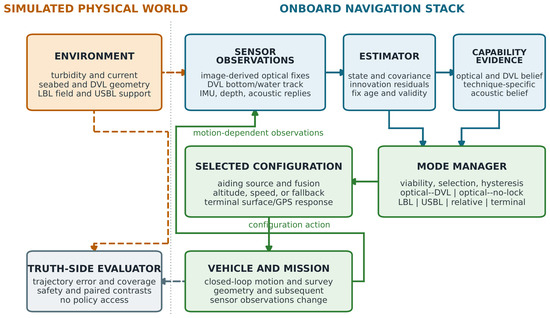
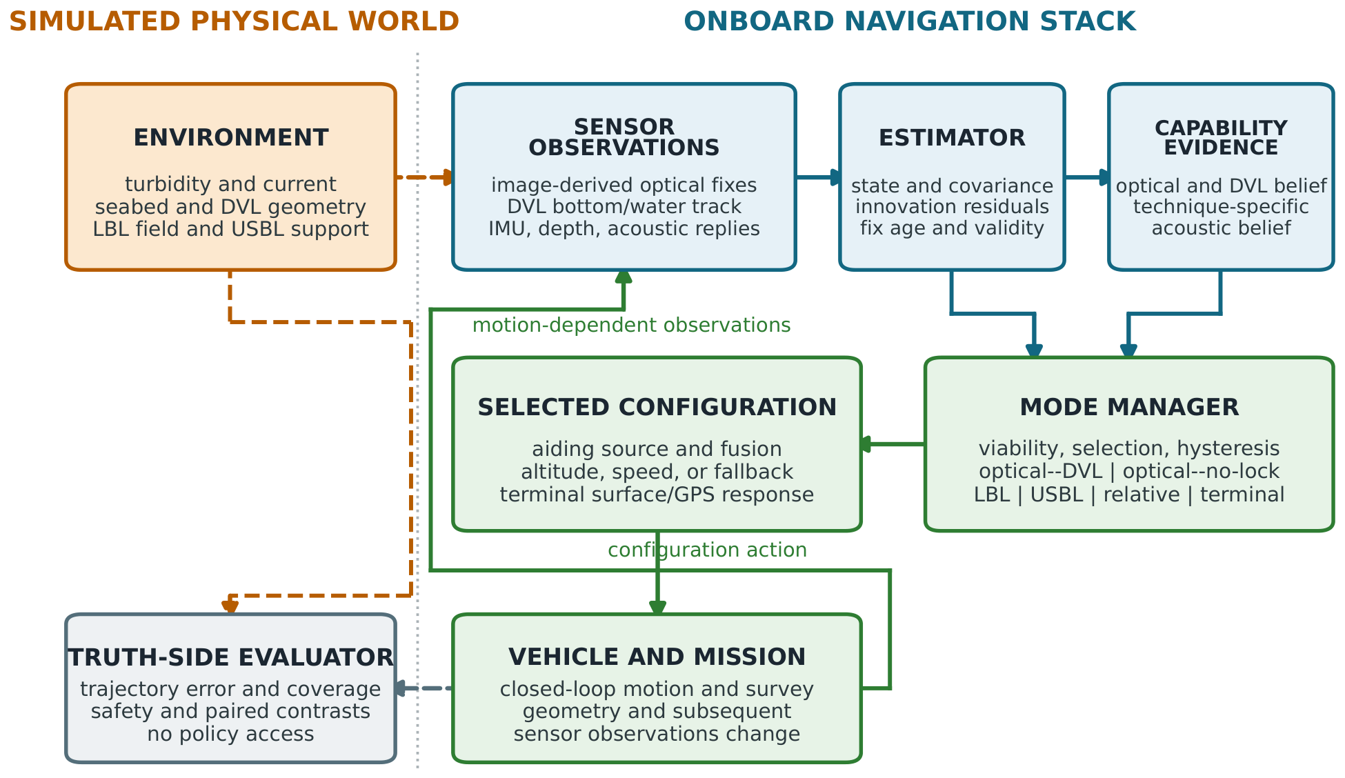
The provided environment includes a deterministic headless simulator for performing paired experiments, as well as a ROS 2/Gazebo demo for visual inspection. Only headless runs yield quantitative data. In every simulation step, the physical world generates sensor readings, the estimator and mode manager process only locally observable inputs, control outputs are sent to the vehicle, and the resulting vehicle pose creates the next batch of measurements. Only simulator ground truth is stored for offline assessment. This data flow is shown in Figure 1. The quantitative simulator and analysis were implemented in Python 3.12.3 (Python Software Foundation, Wilmington, DE, USA) with NumPy 1.26.4; figures were generated with Matplotlib 3.6.3. ROS 2 Jazzy Jalisco and Gazebo Harmonic 8.15.0 (Open Robotics, Mountain View, CA, USA) support the visual demonstration only and were not used to generate the quantitative results.

Figure 1. Closed-loop mode-aware navigation architecture. Solid blue paths are the onboard-observable information available to the estimator and policy; green paths are consequential configuration and vehicle actions. Orange variables are the latent simulator state. They reach only sensor generation and the truth-side evaluator through dashed paths, never the policy.

Going clockwise around the left-hand side of Figure 1, the environment block contains the latent state: turbidity and current, seabed and DVL geometry, and the deployed LBL field and USBL support. The environment state is not provided to the policy, but only to the sensor models. The sensors produce the observations, consisting of the optical fix based on images, DVL bottom- and water-track returns, and replies from the IMU, depth, and acoustic sensors. The estimator fuses these observations to generate a state and covariance estimate along with the innovation residuals and fix age. These are converted by the capability block into beliefs for optical, DVL, and technique-specific acoustic data. The mode manager determines the feasibility of each option, applies hysteresis, and selects one of the six possible modes. The output of the mode manager is not a mere indication of a mode, but instead specifies the configuration to be implemented. This configuration indicates the aiding source and fusion mode, may affect altitude and speed, and in some cases commits the vehicle to a particular surface-for-GPS terminal response. The vehicle then executes the resulting plan, which changes the geometry and thus produces the subsequent observations and closes the loop. The truth evaluator is not part of the closed-loop system: it has access to both the latent state and the realized trajectory and uses them to calculate error, coverage, safety, and contrast metrics. There is no feedback to the policy from the truth evaluator.

The vehicle performs a survey mission lasting a few minutes in a six-degree-of-freedom environment with depth-dependent pressure measurements, modeled ocean currents, and sensors whose response depends on altitude and velocity. Every paired comparison uses the same reproducible environment and sensor realization for both policies. This common-random-number design reduces extraneous variation, so the paired difference primarily reflects policy behavior rather than unequal disturbances.

3.2. Optical Sensing and Feedback

The optical model follows the direct transmission and scattering framework for underwater image formation [5,6,7,27,28]. With attenuation coefficient c and sensor-to-bottom distance r, the direct two-way path is

$$T(r,c)=\exp (-2cr).$$

(1)

Hence, altitude and water clarity determine if enough seabed texture reaches the camera for a fix. The generated images are forwarded to the chosen P5-v4 image-to-fix front end, and the observable outputs are fix availability, uncertainty, inlier support, reprojection quality and ambiguity diagnostics. The turbidity is not directly communicated to the manager. Instead, the manager receives the optical evidence and its history. This matters because the optical feedback closes a measurement loop rather than issuing a mode command. The optical environment affects the image, the image-based localizer computes availability and uncertainty, and availability and uncertainty impact the manager’s belief in its capabilities. Thus, the optical branch is a part of the navigation process via a real measurement interface, but it is separate from the truth side evaluator.

3.3. DVL, Inertial, and Current Modeling

The bottom tracking Doppler velocity log (DVL) gives a velocity estimate with respect to the seabed, while the water tracking DVL gives an estimate with respect to the water; therefore, the water tracking DVL requires the water motion with respect to ground to recover estimates with respect to ground. Both observations are modeled separately in the implementation. Probability of bottom-lock is a function of vehicle altitude and DVL health, while water-track availability is modeled independently. Scale, alignment, noise, dropout, and full crashout all affect measurement generation instead of setting policy mode directly.

The navigation filter estimates position, velocity, attitude-related error states, sensor biases, and water current. In succinct notation, the prediction and update are given by

$$\begin{array}{cccc}\hfill {\widehat{\mathit{x}}}_k^{-}& =f({\widehat{\mathit{x}}}_{k-1},{\mathit{u}}_k),\hfill & \hfill {\mathit{P}}_k^{-}& ={\mathit{F}}_k{\mathit{P}}_{k-1}{\mathit{F}}_k^{\mathsf{T}}+{\mathit{Q}}_k,\hfill \end{array}$$

(2)

$$\begin{array}{cccc}\hfill {\mathit{r}}_k& ={\mathit{z}}_k-h\left({\widehat{\mathit{x}}}_k^{-}\right),\hfill & \hfill {\mathit{S}}_k& ={\mathit{H}}_k{\mathit{P}}_k^{-}{\mathit{H}}_k^{\mathsf{T}}+{\mathit{R}}_k,\hfill \end{array}$$

(3)

$$\begin{array}{cccc}\hfill {\mathit{K}}_k& ={\mathit{P}}_k^{-}{\mathit{H}}_k^{\mathsf{T}}{\mathit{S}}_k^{-1},\hfill & \hfill {\widehat{\mathit{x}}}_k& ={\widehat{\mathit{x}}}_k^{-}+{\mathit{K}}_k{\mathit{r}}_k.\hfill \end{array}$$

(4)

Here, k is the discrete time index and ${\widehat{\mathit{x}}}_k$ is the estimated state, comprising position, velocity, attitude-related error states, sensor biases, and water current; the superscript "—" denotes the prior value, obtained before the measurement update. The function $f\left(·\right)$ is the process model and ${\mathit{u}}_k$ the commanded input, with ${\mathit{F}}_k$ being its Jacobian evaluated at the current estimate. The matrix ${\mathit{P}}_k$ is the state error covariance and ${\mathit{Q}}_k$ the process noise covariance. On the update side, ${\mathit{z}}_k$ is the measurement, $h\left(·\right)$ the measurement model, ${\mathit{H}}_k$ its Jacobian, and ${\mathit{R}}_k$ the measurement noise covariance. The residual ${\mathit{r}}_k$ is the innovation, ${\mathit{S}}_k$ its covariance, and ${\mathit{K}}_k$ the Kalman gain.

Delayed acoustic measurements are applied using fixed-lag replay such that the time at which they are valid determines the corrected state. The Joseph covariance form is used after measurement updates.

3.4. Acoustic Infrastructure and Service Discovery

LBL and USBL exist only if their necessary infrastructure has been deployed. An LBL fix additionally depends on the geometry of the array, range and acoustic conditions. A USBL fix additionally depends on the presence and relative geometry of the supporting surface asset. A single beacon can only provide range-only information, and hence is not considered a complete absolute position. Service identity may be loaded from legitimate pre-mission deployment information, but current availability is not free information. The vehicle probes services in sequence, incurs the cost of the observation opportunity, and retains evidence of response for a limited period. A non-responsive or geometrically impossible service therefore drops out of the set of observable candidates once its evidence expires. The same service catalogue is given to deployment-informed FIXED and the adaptive policies.

3.5. Capability Belief

Let $C_j\in \{0,1\}$ denote whether capability j is available and let $o_{1:k}$ be the observation history. The manager maintains

$$b_{j,k}=P(C_j=1\mid {\mathit{o}}_{1:k}),$$

(5)

for optical, velocity, acoustic, and inertial capability. Evidence includes fix availability and age, uncertainty, DVL track status and probability of lock, acoustic response and dilution of precision, delayed-measurement validity and innovation consistency. A capability can only operate if its post-condition exceeds the freeze boundary and the physical observation required by that mode is present. Hysteresis and minimum dwell delay rapid mode switches but allow immediate exit from a mode when the required evidence is no longer present.

3.6. Navigation Modes and Actions

Only combinations that result in different navigation behaviour are included in the finite set of modes (Table 2). The combination does not get expanded into separate modes if there is no distinct behavior. Where the technique identity affects the dependence on infrastructure and what is passed to the estimator it is kept. Recovery actions such as lower altitude, reduce speed, hold for a fix, or surface are secondary actions. When a change in capability occurs the first response is to select another navigation mode that can provide sufficient performance. Recovery is taken as the response only when it is not possible to select another mode to provide sufficient navigation or when a predefined safety condition is reached.

Table 2. Navigation modes selected from onboard-observable evidence.

Mode	Required Observable Evidence	Navigation Behavior
Optical + DVL	Optical fix viable; bottom track live	Optical absolute aiding with ground-relative DVL
Optical, no bottom lock	Optical fix viable; bottom track absent	Optical absolute aiding with water track or inertial velocity propagation
LBL aided	Responding position-giving LBL service	LBL absolute updates with available onboard velocity aiding
USBL aided	Responding position-giving USBL service	USBL absolute updates with available onboard velocity aiding
Relative dead reckoning	No absolute aid; DVL velocity evidence viable	IMU plus bottom/water-track relative navigation; uncertainty grows
Terminal degraded	No viable submerged navigation and safety condition met	Abort submerged survey, surface, reacquire GPS, terminate mission

3.7. Policies and Comparator Fairness

All policies have the same estimator, sensor models, mission controller, initialization, and locked base configuration (lidar optical channel, 5 $\mathrm{m}$ altitude, $0.5 \mathrm{m} {\mathrm{s}}^{-1}$, USBL, covariance weighting). They differ only in the authority shown in Table 3.

Table 3. Policy definitions. Deployment-informed FIXED is the primary comparator because it receives the same legitimate pre-mission infrastructure knowledge as the adaptive policies.

Policy	Permitted Behavior
Universal FIXED	One locked configuration for every environment; retained as a supporting static reference.
Deployment-informed FIXED	Before launch, replaces only the acoustic technique using the deployed-service catalogue; remains fixed afterward and receives no future-event information.
REACTIVE	Uses the same starting configuration and catalogue, then selects modes from current observable evidence online.
PREDICTIVE	REACTIVE plus an observable-history forecast that may initiate a pre-emptive recovery action; secondary comparison with no required success threshold.

Table 4 reports the principal settings used in Study 3. The table groups them as modeled physical quantities, experimental design assumptions, and controller or estimator tuning values.

Table 4. Principal Study 3 simulation, sensor, estimator, and mode-manager parameters.

Group and Parameter	Value	Status
Mission: horizon/policy/image period	180/2/4 s	Design assumptions
Mission: fixed altitude/speed	5.0 m/0.5 m s−1	Controller settings
Optical: image/horizontal field of view	$192\times 192$ px/${60}^{\circ }$	Simulation model
Optical: AKAZE threshold/match ratio	$5\times {10}^{-5}$/0.80	Algorithm tuning
Optical: inliers/fraction/reprojection	12/0.50/2.0 px	Admission tuning
Optical: accepted scale/covariance factor	0.60–1.67/2.30	Admission tuning
DVL: bottom-/water-track noise	0.015/0.025 m s−1 × scale	Modeled noise
Depth: generated noise/filter $\sigma$	0.015/0.01 m	Model/estimator tuning
Current: random walk	0.003 m ${\mathrm{s}}^{-1}/\sqrt{\mathrm{s}}$	Estimator model
Acoustic: probe period/evidence lifetime	4/8 s	Service-discovery design
Acoustic: delay/jitter $\sigma$	0.08/0.02 s	Modeled communication
Acoustic: LBL calibration/filter $\sigma$	0.02/0.35 m	Model/estimator tuning
Estimator: state/fixed lag/NIS gate	12 states/15 s/9.0	Structure/tuning
Estimator: reacquisition inflation/confirms	25/2	Estimator tuning
Manager: usable boundary/minimum hold	0.35/8 s	Controller tuning
Manager: optical floor/evidence window	0.25/4 observations	Controller tuning
Manager: recovery dwell/cooldown	8/48 s	Controller tuning
Environment: turbidity-like process	[0.05, 0.90], mean 0.45	Dimensionless simulation model
Environment: east/north current	$\pm 0.18$/$[-0.20,0.20]$ m s−1	Modeled physical quantities
Environment: acoustic noise	[45, 80] dB, mean 61 dB	Modeled quantity
Environment: bottom-lock reference/width	4.5/0.55 m	Simulation model

3.8. Experimental Progression

Studies 1 and 2 provided the groundwork for the final mode-aware evaluation by characterizing the navigation-configuration space, identifying the conditions under which adaptation matters, and establishing the role of navigation-level action (Table 5). Their full results and artifacts are available from the public repository referenced in the Data Availability Statement.

Table 5. Empirical foundation provided by the Study 1 and Study 2 characterization experiments. Development-stage objective values characterize the design process and are not final Study 3 performance evidence.

Study	Key Finding	Quantitative Evidence	What It Established
Study 1—configuration and design-space characterization	Navigation performance depended substantially on configuration, with no single configuration universally preferable across the investigated conditions.	144 configurations × 10 scenarios × 19 failure families = 27,360 runs. Development objective: $J=0.081$ for the adaptive configuration and $J=0.017$ for the selected fixed configuration.	Configuration choice materially affects navigation performance and should be treated as an explicit navigation-design problem rather than assuming one universally appropriate sensing configuration.
Study 2—failure and architecture characterization	Most failure conditions did not require policy differentiation, while a smaller subset exposed conditions in which navigation capability genuinely needed to change. Measurement admission or reweighting alone did not reproduce the recovery obtained through capability, guidance, and mission-level action.	19 failure families: 13/19 non-discriminating and 6/19 policy-discriminating.	Adaptation should be selective rather than continuous, and some capability-loss conditions require navigation-level action beyond estimator-level measurement weighting.

These studies led to the central question for Study 3: Is there benefit to online adaptation when the adaptive action is based on observable evidence of capability change, compared to a strong deployment-informed fixed configuration when the change in capability occurs after launch? Study 3 provides the primary evidence, with explicitly mixed infrastructure, observable service discovery, and deployment-informed FIXED as the primary comparator.

The final Study 3 evaluation used the corrected controller in two complementary parts. Part A comprised 270 paired scripted cases: seven transition families with 30 realizations per policy and three controls with 20 realizations each. Part B comprised 400 paired, previously unseen dynamic environments per policy. Turbidity, currents, DVL health, acoustic noise and geometry, and infrastructure availability evolved through reproducible stochastic processes. Every policy encountered the same matched environmental realization, but none received its hidden process state or future evolution. Parts A and B address different questions and are therefore analysed separately.

3.9. Metrics and Statistical Analysis

The main Part B criterion was (i) lower REACTIVE horizontal RMSE than deployment-informed FIXED, with the paired 95% confidence interval entirely below zero, and (ii) the replay-verified adequate viable-mode adaptation greater than 50%. Secondary outcomes included transition RMSE, peak error, unaided time, longest aiding gap, completion, safety violations, survey coverage, mode switches, and physical interventions. For Part B, 95% paired bootstrap intervals were computed with 10,000 bootstrap draws. Part A used a family-stratified paired bootstrap to preserve the representation of each scripted family. The bootstrap procedure, metrics, comparators, sample sizes, and decision rules were specified before the final evaluation.

An adequate adaptation is defined as selecting any currently viable mode with contemporaneous supporting evidence. We evaluate the exact preferred-mode adaptation only if the objective specifies exactly one preferred mode; simultaneous viable modes are treated as ambiguous otherwise.

The complete evaluation archive passed checksum verification, and sampled traces were reproduced exactly from the recorded inputs. Detailed execution and integrity records are provided in the supplementary reproducibility material.

4. Results

4.1. Foundational Studies and Comparator

Studies 1 and 2 show that we were able to reproduce a closed-loop environment which includes optical impairment, DVL dropouts, intermittent acoustics, infrastructure collapse, current, multiple simultaneous faults, and the end condition of streams running together. Furthermore, they show why there cannot be a single reference configuration that applies universally. Specifically, in Study 2’s held-out block, the manager performed well above the admission-only ablation but it did not perform better than the best predeclared fixed configuration on the aggregate metric. This negative result altered the final question from “Can adaptation outperform one fixed choice?” to “Can online adaptation outperform the best configuration that we could choose given knowledge of our deployment context?”. Study 3 tests that question.

A Study 3 held-out block ran previously at an independent root and remains preserved as a separate historical result. That run employed the precorrection controller, and its results indicated that REACTIVE was significantly better than universal FIXED ($-0.4374 \mathrm{m}$, 95% CI [$-0.4628 \mathrm{m}$, $-0.4122 \mathrm{m}$]), but performed similarly to deployment-informed FIXED ($-0.0070 \mathrm{m}$, 95% CI [$-0.0197 \mathrm{m}$, $0.0061 \mathrm{m}$]). Further investigation revealed the reason for this performance: inaccurate service information, as well as non-compliance with terminal safety requirements. The corrected controller was then tested on a different independent root. The results of these two controllers were not combined.

4.2. Scripted Held-Out Robustness: Part A

In Part A, deployment-informed FIXED, REACTIVE, and PREDICTIVE all achieved 0.8519 completion. Deployment-informed FIXED and REACTIVE had zero safety violations in the 270 cells, while PREDICTIVE had one safety violation. The mean horizontal RMSE was $0.5521$ $\mathrm{m}$ for deployment-informed FIXED and $0.5588$ $\mathrm{m}$ for REACTIVE. The difference between these two metrics was $0.0067$ $\mathrm{m}$ (95% CI $-0.0073$ $\mathrm{m}$ to $0.0212$ $\mathrm{m}$). The confidence intervals of the transition RMSE, peak error, and maximum aiding gap all included zero. On the test set, REACTIVE simply reproduced the performance of the deployment-informed configuration rather than improving it, at the cost of 6.15 mode switches per mission. This is the edge case where our script typically does not compel us to deploy any other configuration than the one we would have deployed anyway. Table 6 summarizes the held-out means for both experimental parts.

Table 6. Final corrected-controller held-out means. Parts A and B are separate experimental blocks and are not pooled.

Part	Metric	Deploy-FIXED	REACTIVE	PREDICTIVE
A	Completion	0.8519	0.8519	0.8519
A	Safety violation	0.0000	0.0000	0.0037
A	Overall RMSE (m)	0.5521	0.5588	0.5652
A	Mode switches	0.0000	6.1481	5.9556
B	Completion	0.4175	0.4325	0.4275
B	Safety violation	0.2325	0.1500	0.1725
B	Overall RMSE (m)	2.3508	1.9245	1.9803
B	Transition RMSE (m)	2.4409	2.0004	2.0798
B	Peak error (m)	5.7444	4.8584	4.9376
B	Longest aiding gap (s)	46.9800	40.7100	42.7650
B	Survey coverage	0.8478	0.8163	0.8414
B	Mode switches	0.0000	8.3150	8.7350
B	Physical interventions	0.5825	6.4450	7.5025
B	Pre-emptive actions	0.0000	0.0000	0.5225

4.3. Dynamically Changing Held-Out Environments: Part B

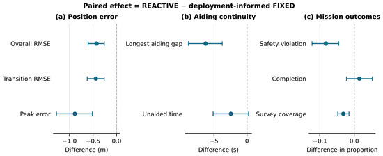
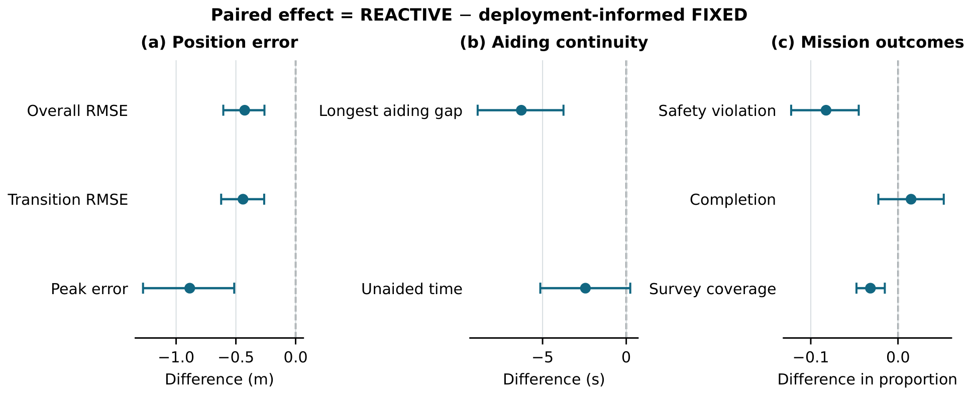
For Part B, REACTIVE brought down mean horizontal RMSE from $2.3508$ $\mathrm{m}$ to $1.9245$ $\mathrm{m}$. The paired difference was $-0.4262$ $\mathrm{m}$ and the whole 95% confidence interval [ $-0.6052$ $\mathrm{m}$, $-0.2608$ $\mathrm{m}$] favored REACTIVE, which means the first requirement of the predeclared primary criterion was met. The advantage also applied to transition RMSE ($-0.4405 \mathrm{m}$), peak error ($-0.8860 \mathrm{m}$), longest aiding gap ($-6.27 \mathrm{s}$), and frequency of safety violations ($-0.0825$): all four confidence intervals excluded zero on the side favoring REACTIVE (Table 7, Figure 2). The unaided-time difference was $-2.44$ $\mathrm{s}$ but the confidence interval included zero. Completion improved by 0.0150 with a confidence interval including zero; so there is no claim of completion advantage.

Table 7. Part B paired effects, REACTIVE minus deployment-informed FIXED. Negative differences favor REACTIVE for error, aiding-gap, and safety-violation metrics; positive differences favor REACTIVE for completion and survey coverage. Mode-switch and intervention differences quantify adaptation cost.

Metric	Mean Difference	95% CI Low	95% CI High
Overall RMSE (m)	−0.4262	−0.6052	−0.2608
Transition RMSE (m)	−0.4405	−0.6231	−0.2632
Peak error (m)	−0.8860	−1.2768	−0.5138
Longest aiding gap (s)	−6.2700	−8.8800	−3.7500
Safety violation	−0.0825	−0.1225	−0.0450
Unaided time (s)	−2.4400	−5.1350	+0.2402
Completion	+0.0150	−0.0225	+0.0525
Survey coverage	−0.0316	−0.0476	−0.0151
Mode switches	+8.3150	+7.9725	+8.6625
Physical interventions	+5.8625	+5.6025	+6.1225

Figure 2. Part B paired effects, defined as REACTIVE minus deployment-informed FIXED and shown in their native units. Negative values favor REACTIVE for position error, aiding-gap duration, and safety violations; positive values favor REACTIVE for completion and survey coverage. Numeric effects and 95% confidence intervals are given in Table 7; the dashed zero lines denote no paired difference.

All paired effects are expressed as REACTIVE minus deployment-informed FIXED. Thus, a negative sign means REACTIVE achieved a smaller value, which is advantageous for error, aiding-gap duration, unaided time, and safety violations. A positive sign means REACTIVE achieved a larger value, which is advantageous for completion and coverage, but implies more action for mode switches and physical interventions. The sign indicates only the direction of arithmetic comparison; whether it is advantageous or disadvantageous depends on what is being measured.

Reading Figure 2 panel by panel, the three groups separate the kinds of outcome rather than mixing them on one axis. Panel (a) covers position error, where overall RMSE, transition RMSE, and peak error all sit left of the dashed zero line with their intervals clear of it, so REACTIVE is more accurate on every error measure. Panel (b) covers aiding continuity. The longest aiding gap is shortened and its interval excludes zero, whereas the unaided-time interval crosses the line, so the gain is in the length of the worst gap rather than in the total time spent without an absolute fix. Panel (c) covers mission outcomes, and it is the panel that shows the trade-off. Safety violations fall with an interval clear of zero, completion moves slightly but its interval spans the line and supports no claim, and survey coverage falls with its interval clear of zero, which is a cost rather than a benefit. Each marker is the paired mean difference and each bar the 95% confidence interval, so a bar that touches the dashed line indicates an effect the data do not separate from no difference.

4.4. Illustrative Capability Transition

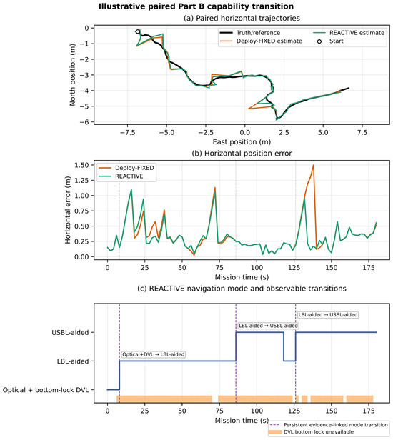
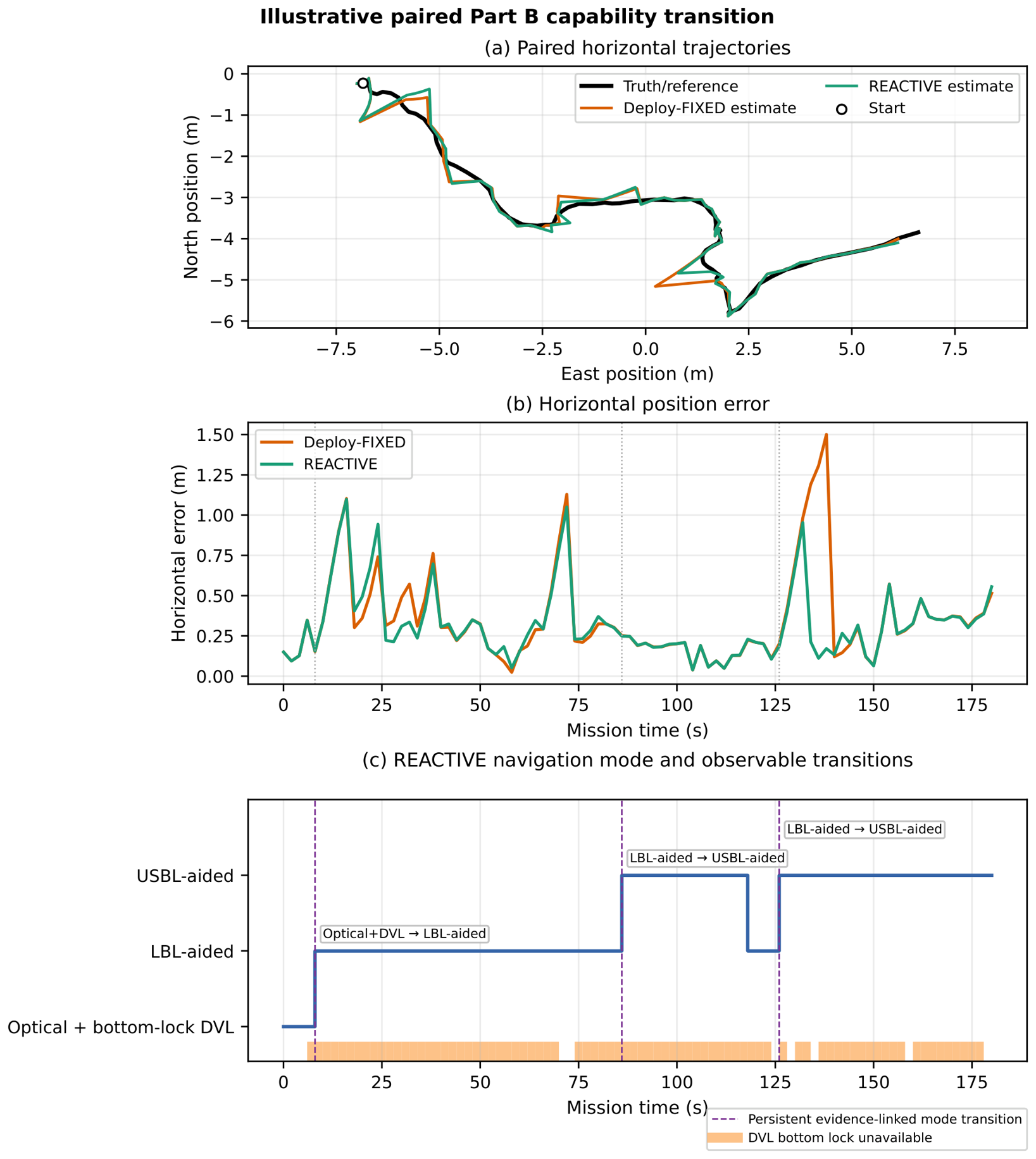
Figure 3 illustrates how mode adaptation operates during a typical Part B mission. The case was selected objectively before plotting: among missions containing a persistent, evidence-linked mode transition, it had a paired RMSE effect closest to the median. Accordingly, it represents the central tendency of the observed accuracy improvement rather than a particularly favorable example. Deployment-informed FIXED and REACTIVE achieved horizontal RMSE values of $0.4572$ $\mathrm{m}$ and $0.3871$ $\mathrm{m}$, respectively; their difference of $-0.0701$ $\mathrm{m}$ closely matches the eligible-set median of $-0.0714$ $\mathrm{m}$.

Figure 3. Illustrative paired Part B realization selected objectively before plotting. (a) Common truth/reference trajectory and the deployment-informed FIXED and REACTIVE estimates. (b) Horizontal position error versus mission time. (c) REACTIVE navigation mode, persistent evidence-linked transitions, and DVL bottom-lock unavailability. The complete time history is shown without omission. The figure illustrates mechanism behavior; aggregate claims are based on all 400 paired dynamic environments.

Both policies encounter the same environment and reference trajectory. At the start, REACTIVE uses optical positioning with bottom-track DVL. When bottom lock is lost, it transfers absolute aiding to LBL while retaining the available onboard propagation. Later, changing acoustic-service evidence leads it to use USBL. The trajectory and error panels show the navigation consequence of these transitions, while the mode timeline links each change to observable evidence. This mission is illustrative; all aggregate effects and confidence intervals remain based on the complete paired evaluation of 400 dynamic environments. Replay and integrity details are provided in the supplementary reproducibility record rather than used as part of the scientific interpretation.

4.5. Supplementary Parameter Sensitivity

This subsection reports a supplementary analysis conducted separately from the primary Study 3 evaluation. The held-out evaluation of Section 4.2 and Section 4.3 remains the basis for the statistical claims of this paper; the analysis reported here characterizes parameter dependence without altering it. We executed a supplementary sensitivity analysis on an independent set of 60 fresh paired generated environments that does not overlap any earlier study. These environments were evaluated with FIXED (deployment-informed), nominal REACTIVE, and ten single-parameter REACTIVE variants, for a total of 720 simulations. We varied only the usable capability boundary, minimum hold, optical-quality floor, recovery dwell, and recovery cooldown parameters at their predeclared low and high values. The protocol, including the sample size and material-reversal rule below, was fixed prior to execution; all 720 runs finished with no retry and no exclusion. Table 8 reports each change as $\Delta M=M_{\mathrm{variant}}-M_{\mathrm{nominal}}$, where nominal denotes the unmodified REACTIVE policy. $\Delta$RMSE and $\Delta$Trans. are changes in overall and transition horizontal RMSE, respectively, in metres; $\Delta$Comp., $\Delta$Safety, and $\Delta$Coverage are changes in mission completion, safety-violation, and survey-coverage proportions; and $\Delta$Switch and $\Delta$Interv. are changes in the mean numbers of mode switches and physical interventions per mission. Thus, negative RMSE, transition-RMSE, and safety differences favor the variant, whereas positive completion and coverage differences favor it. Switch and intervention differences describe controller activity and are not intrinsically beneficial or adverse. No parameter of the proposed method was re-optimized as a consequence of this analysis, and the original held-out results were not reused for optimization or replacement.

Table 8. One-at-a-time sensitivity relative to nominal REACTIVE on 60 fresh paired environments. Negative RMSE differences favor the variant; completion and safety columns are changes in proportions.

Variant	$\Delta$RMSE	$\Delta$Trans.	$\Delta$Comp.	$\Delta$Safety	$\Delta$Coverage	$\Delta$Switch	$\Delta$Interv.
Capability boundary 0.30	−0.001	−0.002	+0.017	0.000	+0.000	−0.03	−0.03
Capability boundary 0.40	+0.007	+0.007	−0.017	0.000	−0.002	−0.07	+0.08
Minimum hold 4 s	−0.040	−0.044	+0.033	0.000	+0.030	+1.40	+2.00
Minimum hold 12 s	−0.238	−0.248	+0.067	−0.033	+0.031	−0.22	−0.78
Optical floor 0.20	−0.002	−0.002	0.000	0.000	−0.000	0.00	+0.02
Optical floor 0.30	+0.034	+0.034	0.000	0.000	+0.003	0.00	+0.03
Recovery dwell 4 s	+0.032	+0.031	+0.017	+0.017	+0.017	+0.17	+0.10
Recovery dwell 12 s	−0.044	−0.044	0.000	−0.017	−0.010	−0.08	+0.17
Recovery cooldown 32 s	−0.006	−0.007	−0.017	0.000	0.000	−0.03	+0.17
Recovery cooldown 64 s	−0.002	−0.002	0.000	0.000	−0.000	−0.02	−0.08

The nominal REACTIVE achieved an overall RMSE of $1.608$ $\mathrm{m}$ on these 60 environments, versus $2.092$ $\mathrm{m}$ for deployment-informed FIXED; their paired difference was $-0.485$ $\mathrm{m}$ (95% paired bootstrap interval [ $-0.978$ $\mathrm{m}$, $-0.002$ $\mathrm{m}$]). Its safety-violation proportion was lower by 0.150 [–0.267, –0.033], while the completion difference of −0.017 [–0.117, 0.083] was inconclusive. None of the bounded settings activated the predeclared qualitative-reversal rule. Capability boundary, optical floor, recovery dwell, and cooldown produced mostly small or uncertain effects. The minimum hold time showed the most sensitivity, with shortening it increasing the number of switches and interventions, and lengthening it decreasing them and lowering the point estimate of RMSE, though its RMSE difference from the nominal had a 95% interval including zero. This analysis indicates that the direction of the central comparison was robust across the five parameters and ranges evaluated here, and identifies selector persistence as the parameter governing the responsiveness and stability trade-off. Its scope is the tested ranges and the simulated environment distribution used throughout this work; it characterizes parameter dependence rather than establishing an optimal setting.

4.6. Adaptation Behavior and Costs

Replay-based analysis revealed 2704 REACTIVE episodes where it would have been possible to judge the quality of a persistent viable-mode decision. REACTIVE chose a viable mode that was justified by evidence contemporaneous with the episode in 1913 of those cases, or 70.75%. This is above the 50% threshold declared beforehand and fulfils the second requirement of the primary claim. If the goal specified one specific preferred mode, then exact adaptation occurred in 57.53% (974 out of 1693) of cases. Using the older unchanged definition of V5 C7/C8 (which applies a different denominator and interprets “persistence” differently), exact adaptation occurred in 59.17% (1290 out of 2180) of cases. These values are calculated independently and cannot be substituted for one another.

The gain from improved navigation came with a trade-off. As compared to FIXED with deployment knowledge, REACTIVE added 8.32 mode changes and 5.86 physical interventions on average per Part B mission. The amount of area surveyed fell by 0.0316 on average, and its 95% confidence interval did not contain zero. In effect, there was a compromise between responsiveness and stability because the agent spent time adjusting or stabilizing the navigation state, lowering error and violations of safety rules but marginally decreasing the area surveyed.

Mission completion was challenging under these conditions: FIXED had a success rate of 0.4175, while REACTIVE achieved 0.4325, and safety violations occurred in 23.25% and 15.00% of missions, respectively. REACTIVE therefore improved on FIXED under identical conditions.

4.7. PREDICTIVE

The PREDICTIVE policy executed 0.5225 anticipatory actions on average per mission in Part B, and 1.10 per mission in Part A, suggesting that the predictive arm of the algorithm was active. It did not beat REACTIVE, however. The difference between its Part B RMSE and REACTIVE’s was $0.0558$ $\mathrm{m}$ (95% CI [ $-0.0352$ $\mathrm{m}$, $0.1491$ $\mathrm{m}$]); unassisted time rose by $4.515$ $\mathrm{s}$ [ $1.900$ $\mathrm{s}$, $7.1851$ $\mathrm{s}$]; maximum aiding gap increased by $2.055$ $\mathrm{s}$ [ $0.460$ $\mathrm{s}$, $3.715$ $\mathrm{s}$]; and interventions rose by 1.0575 [0.8250, 1.3050]. These improvements resulted from reactive adjustments to the current situation; the forecast made available to this experiment did not yield any further benefit.

5. Discussion

5.1. Operating Regime of Online Adaptation

The remaining data frames the operating range for the method proposed in this study. For Part A, the FIXED policy with knowledge of the deployment was adequate and REACTIVE was unable to realize an accuracy benefit by switching between alternatives that were approximately equivalent in utility. In Part B, the environment changes after launch: visibility, DVL operation, acoustic quality and geometry, currents, and infrastructure availability change during the course of a mission. No single configuration is optimal across all possible realizations. REACTIVE reduces overall and transition errors, peak errors, aiding gaps, and safety violations.

The difference between blocks is more scientifically informative than a pooled mean, because it demonstrates that online adaptation is not inherently useful simply by virtue of being available. Its usefulness becomes evident when changing observations suggest that a particular alternative is better, and this constitutes a change in viable navigation configuration. This conditional result is consistent with the physical structure of underwater sensing: optical, DVL, and acoustic capabilities are lost and recovered for different reasons.

5.2. Interpretation of Adaptation Rates

The 70.75% adequate rate measures whether the policy selected any defensible viable mode supported by evidence at the time. This is the appropriate primary mechanism measure when several absolute modes are simultaneously viable and no predeclared objective orders them. The lower 57.53% exact rate applies only to episodes with a unique preferred mode and reveals room for improvement in service probing, belief latency, and selector discrimination. Neither rate implies perfect diagnosis, and neither uses mode labels supplied by the simulator. The V5-definition value of 59.17% is lower because it answers a related but different question with a different episode construction. Reporting both avoids turning analysis convention into apparent algorithmic performance. The replay-verified adequate measure is tied directly to the final decision rule; the V5 measure preserves continuity with earlier development analysis.

5.3. Navigation Resilience and Mission Efficiency

The reductions in safety violations, peak error, and aiding gaps demonstrate that mode awareness improved navigation resilience under changing capability. The manager does not simply re-weight measurements; it changes the operational configuration as optical, DVL and acoustic evidence changes. If there is another viable modality, then this maintains a better-bounded navigation solution, whereas if submerged navigation is no longer possible, then the terminal behaviour avoids extended operation on an unbounded estimate.

These gains come at a cost of 5.86 more physical actions per mission and 0.0316 less survey coverage. This is a trade-off in the engineering design rather than a contradiction of the navigation result. Changes to the sensing configuration, altitude, speed or mission behaviour take time, and they may require more energy for propulsion, sensing and computation. In the current experiments, we measured time and coverage, but energy was not an objective. The results show that adaptation can improve navigation and safety when sensing capability changes after launch, and suggest that an explicit model of the cost of switching modes should be part of future autonomous vehicle design.

In both strategies, completion is challenging because each leads to situations where there is no feasible underwater horizontal aid available. Continuing the mission in these situations would imply operation without a sufficiently bounded navigation solution. The terminal mode gives a safety bound in these cases. Future implementations can use this to explicitly decide whether a mission failure is recoverable or not, and support restarting the mission once back on the surface with access to satellite GPS.

5.4. Relationship to Existing Research

Adaptation at the system level complements adaptive covariance filtering and robust gating, which work within a mode and determine how much each measurement affects the navigation solution. The system-level approach described here determines what physical configuration should produce and fuse these measurements. Likewise, active perception approaches alter the distance, relative orientation or illumination to keep a sensory task [17,18]. Nonetheless, the control manager presented here can transition between optical, velocity-aided, infrastructure-dependent acoustic, relative positioning, and terminal modes in response to changes in perceived sensor capability of each mode.

The predictive variant of the policy provides additional capability over this architecture. Although it tries to preemptively reconfigure itself before a failure occurs, demonstrating that forecasting is feasible, it does not improve over the direct reactive strategy for the cases tested. Spatial texture changes might look analogous to temporal variations in optical transparency, or sudden failures may not exhibit sufficient warning. Therefore, the main contribution is in reactive mode selection, which delivers the stated navigation and safety improvements with no advance notice of environmental changes. Forecasting may be beneficial in situations where predictions are accurate and the expense of action can be easily quantified.

5.5. Limitations and Future Rresearch

The evidence in this paper is entirely simulation-based. It supports claims about closed-loop behavior within the implemented distributions, not field performance, certification, or transfer to arbitrary vehicles and sites. The evaluation environment is a quantitative closed-loop simulation rather than a visualization or a replay of prerecorded data: optical, DVL, depth, and acoustic measurements are generated from the evolving environment and vehicle state, the estimator consumes them, the resulting navigation solution drives guidance and mode selection, and those decisions change the vehicle state and therefore the measurements available at the next step. Both policies were exercised on identical generated realizations, so the reported paired differences are attributable to the policy rather than to the environment draw. Each component of that loop is a model rather than a site measurement. DVL bottom/water-track availability, acoustic propagation and packet response, infrastructure geometry, currents, and vehicle motion are bounded models rather than a site-specific survey. The reported error, completion, coverage, and safety rates therefore characterize behavior within the implemented distributions rather than a particular deployment.

Translation to a vehicle requires staged calibration and validation: camera and optical-quality calibration using site/field imagery; DVL lock and noise characterization over altitude and terrain; LBL/USBL latency, geometry, and outlier measurements; vehicle hydrodynamic and energy identification; hardware timestamp and compute-latency tests; and finally controlled-water followed by field trials with independent safety supervision. Such tests should retain the observable-only policy boundary and compare against a deployment-informed fixed configuration under matched disturbances.

The most significant operational limitation occurs when optical positioning, acoustic aid for position, and functional DVL measurements are all unavailable. No algorithmic solution exists to recover horizontal observability when all capabilities are absent. The implemented terminal state handles this case by ceasing dangerous underwater movement and transitioning into the designated surface ascent sequence. Future research should address the higher-level actions associated with such a response, including GPS position recovery, route re-evaluation, established protocols for dealing with these events, and whether and how to resume or cease the survey.

Changes in configuration also have an unknown endurance cost within the bounds of the reported experiments. Going up or down, and going faster all demand more propulsive power; optical and acoustic sensors require electrical power; more additional onboard computing and communications increase hotel-load power consumption; and switching modes might reduce the overall time-on-station. Energy consumption and battery state-of-charge should be measured and optimized along with localization precision, spatial coverage, and hazard avoidance in future work. This will allow transition decisions to weigh the physical cost of each choice while continuing to prioritize position over power conservation.

More experimentation is needed as well to validate the optical subsystem with images from the field from various bottom types, illumination levels, and turbidity, and to evaluate the effect of stale acoustic updates and current estimates with other types of deployments. The synthetic spaces are deliberately challenging and come from one particular family of stochastic models, so the generality of the safety and mission-success results across different vehicles, environments, and missions remains to be established. This work establishes an explicit transition from the simulation presented here to testing and optimizing power-aware fusion in the field.

6. Conclusions

We designed and evaluated a multimodal navigation framework for an autonomous underwater vehicle that switches between optical, DVL/inertial, and acoustic/localization-dependent modes based on available on-board measurements. We integrated acoustic and estimator evidence into a consequential navigation-mode selection policy. Compared to a strong fixed-configuration baseline informed by the deployment, reactive adaptation reduced the horizontal RMSE by $0.4262$ $\mathrm{m}$ in 400 unseen, dynamically changing environments, where the 95% paired interval did not include zero. It also improved transition error, peak error, aiding continuity, and the rate of safety violations, and selected an adequate viable mode in 70.75% of evaluable persistent adaptation episodes.

In the scripted held-out block, REACTIVE maintained localization accuracy similar to that of a strong pre-mission setting. When the capability changed post-launch, the same architecture gave an advantage. The tested predictive extension was no better than the reactive evidence-based adaptation, which puts the demonstrated contribution in the reactive mode-selection mechanism. In summary, the results indicate that online mode awareness is a viable navigational layer for dynamic underwater sensing conditions, and lay the groundwork for mission rescue, in situ testing, and endurance-aware reconfiguration.

References

- Damari, G.; Yampolsky, Z.; Cohen, N.; Sahoo, A.K.; Danial, J.; Silva, F.O.; Klein, I. AI-Aided Advancements in Autonomous Underwater Vehicle Navigation. arXiv 2026, arXiv:2605.04672. [Google Scholar] [CrossRef] [Scilit]
- Paull, L.; Saeedi, S.; Seto, M.; Li, H. AUV Navigation and Localization: A Review. IEEE J. Ocean. Eng. 2014, 39, 131–149. [Google Scholar] [CrossRef] [Scilit]
- Kinsey, J.C.; Eustice, R.M.; Whitcomb, L.L. A survey of underwater vehicle navigation: Recent advances and new challenges. In Proceedings of the IFAC Conference on Manoeuvring and Control of Marine Craft (MCMC); IFAC: Amsterdam, The Netherlands, 2006. [Google Scholar]
- Tal, A.; Klein, I.; Katz, R. Inertial Navigation System/Doppler Velocity Log (INS/DVL) fusion with partial DVL measurements. Sensors 2017, 17, 415. [Google Scholar] [CrossRef] [Scilit]
- Jaffe, J.S. Underwater optical imaging: The design of optimal systems. Oceanography 1988, 1, 40–41. [Google Scholar] [CrossRef] [Scilit]
- Jaffe, J.S. Computer modeling and the design of optimal underwater imaging systems. IEEE J. Ocean. Eng. 1990, 15, 101–111. [Google Scholar] [CrossRef] [Scilit]
- McGlamery, B.L. A computer model for underwater camera systems. In Proceedings of the Ocean Optics VI; SPIE: Bellingham, WA, USA, 1980; Volume 208, pp. 221–231. [Google Scholar] [CrossRef] [Scilit]
- Schettini, R.; Corchs, S. Underwater image processing: State of the art of restoration and image enhancement methods. EURASIP J. Adv. Signal Process. 2010, 2010, 746052. [Google Scholar] [CrossRef] [Scilit]
- Cohen, N.; Klein, I. BeamsNet: A Data-Driven Approach Enhancing Doppler Velocity Log Measurements for Autonomous Underwater Vehicle Navigation. Eng. Appl. Artif. Intell. 2022, 114, 105216. [Google Scholar] [CrossRef] [Scilit]
- Cohen, N.; Klein, I. Adaptive Kalman-Informed Transformer. arXiv 2024, arXiv:2401.09987. [Google Scholar] [CrossRef] [Scilit]
- Reis, J.; Morgado, M.; Batista, P.; Oliveira, P.; Silvestre, C. Design and Experimental Validation of a USBL Underwater Acoustic Positioning System. Sensors 2016, 16, 1491. [Google Scholar] [CrossRef] [Scilit]
- Rypkema, N.R.; Singh, K. Hybrid Long/Inverted Ultra-Short Baseline (LBL-iUSBL) Acoustic Pose Estimation for Underwater Sonar Mapping. IEEE J. Ocean. Eng. 2025, 50, 1616–1625. [Google Scholar] [CrossRef] [Scilit]
- Pick, D.; Wolbrecht, E.; Anderson, M.; Edwards, D.; Canning, J. Uncertainty Analysis of Ultra-Short- and Long-Baseline Localization Systems for Autonomous Underwater Vehicles. In Proceedings of the OCEANS 2018 MTS/IEEE Charleston, Charleston, SC, USA, 22–25 October 2018; pp. 1–6. [Google Scholar] [CrossRef] [Scilit]
- Williams, T.; Torshizi, K.; Tokekar, P. When to Localize? A POMDP Approach. arXiv 2024, arXiv:2411.08281. [Google Scholar]
- Ferrera, M.; Moras, J.; Trouvé-Peloux, P.; Creuze, V. Real-time monocular visual odometry for turbid and dynamic underwater environments. Sensors 2019, 19, 687. [Google Scholar] [CrossRef] [Scilit]
- Mehra, R.K. On the identification of variances and adaptive Kalman filtering. IEEE Trans. Autom. Control 1970, 15, 175–184. [Google Scholar] [CrossRef] [Scilit]
- Cardaillac, A.; Dansereau, D.G. Learning underwater active perception in simulation. arXiv 2025, arXiv:2504.17817. [Google Scholar] [CrossRef] [Scilit]
- Xanthidis, M.; Kalaitzakis, M.; Karapetyan, N.; Johnson, J.; Vitzilaios, N.; O’Kane, J.M.; Rekleitis, I. AquaVis: A perception-aware autonomous navigation framework for underwater vehicles. In Proceedings of the IEEE/RSJ International Conference on Intelligent Robots and Systems (IROS), Prague, Czech Republic, 27 September–1 October 2021. [Google Scholar]
- Dearden, R.; Ernits, J. Automated fault diagnosis for an autonomous underwater vehicle. IEEE J. Ocean. Eng. 2013, 38, 484–499. [Google Scholar] [CrossRef] [Scilit]
- Chen, Y.; Zhao, Y.X.; Li, S.; He, Y.; Yao, W.; Kayacan, E. Integrated Anomaly Detection, Rollback, and Recovery for Robust INS/DVL Navigation. Ocean Eng. 2025, 342, 122715. [Google Scholar] [CrossRef] [Scilit]
- Davari, N.; Maurelli, F.; Aguiar, A.P. A Robust Navigation System for Underwater Vehicles Using an Adaptive H∞ Filter Based on a Variational Bayesian Approach: Development and Experimental Evaluation. Ocean Eng. 2026, 354, 124719. [Google Scholar] [CrossRef] [Scilit]
- Qin, J.; Li, M.; Li, D.; Zhong, J.; Yang, K. A Survey on Visual Navigation and Positioning for Autonomous UUVs. Remote Sens. 2022, 14, 3794. [Google Scholar] [CrossRef] [Scilit]
- Bao, J.; Mu, X.; Xue, Y.; Zhu, Z.; Qin, H. Robust Multi-Sensor Fusion for Unmanned Underwater Vehicle Navigation. Measurement 2025, 253, 117450. [Google Scholar] [CrossRef] [Scilit]
- Sørensen, F.F.; von Benzon, M.; Pedersen, S.; Liniger, J.; Mai, C. Fault Tree Analysis of Sensor Technologies for Autonomous UUV Navigation. IFAC-PapersOnLine 2022, 55, 484–490. [Google Scholar] [CrossRef] [Scilit]
- Mitchell, A.J.; McGookin, E.W.; Murray-Smith, D.J. Implementation of Sliding Mode Observer Based Reconfiguration in an Autonomous Underwater Vehicle. Acta Polytech. 2005, 45, 18–24. [Google Scholar] [CrossRef] [Scilit]
- Peng, Y.; Xiang, L.; Yang, K.; Jiang, F.; Wang, K.; Wu, D.O. SIMAC: A Semantic-Driven Integrated Multimodal Sensing and Communication Framework. IEEE J. Sel. Areas Commun. 2026, 44, 673–688. [Google Scholar] [CrossRef] [Scilit]
- Gordon, A.; Knittel, M.R. Underwater Multiple Scattering of Light for System Designers; Technical Report TB371; Naval Undersea Center: San Diego, CA, USA, 1973. [Google Scholar]
- Petzold, T.J. Volume Scattering Functions for Selected Ocean Waters; Technical Report SIO Ref. 72–78; Scripps Institution of Oceanography, Visibility Laboratory: San Diego, CA, USA, 1972. [Google Scholar]
Disclaimer/Publisher’s Note: The statements, opinions and data contained in all publications are solely those of the individual author(s) and contributor(s) and not of MDPI and/or the editor(s). MDPI and/or the editor(s) disclaim responsibility for any injury to people or property resulting from any ideas, methods, instructions or products referred to in the content. |
© 2026 by the authors. Licensee MDPI, Basel, Switzerland. This article is an open access article distributed under the terms and conditions of the Creative Commons Attribution (CC BY) license.