Opposing Water-Level Biases of Distributed and Bulk Manning’s Roughness Parameterizations in 2D Modeling of Partly Vegetated Channels: A Patch-Configuration-Dependent Assessment

Abstract

Vegetation is often retained in river channels for habitat conservation and restoration and to facilitate nature-based flood management, and its hydraulic effects are typically represented using flow resistance coefficients in two-dimensional (2D) models. This study evaluated two Manning’s roughness parameterizations in HEC-RAS 2D against large-scale experimental data for grouped and isolated willow patches under high- and low-flow conditions. A distributed approach, which represents spatially varying total resistance using a momentum-based resistance formulation, was compared with a spatially uniform bulk coefficient applied to the entire reach. Because the bulk coefficient was back-calculated from the measured experimental data, it served as an observation-based benchmark rather than an independently derived prediction. A sensitivity analysis established a terrain resolution of 0.001 m and a mesh size of 0.25 m as appropriate for the simulations. The distributed approach consistently underestimated water levels, exhibited an incomplete but directionally correct response to changes in the drag coefficient for grouped patch configurations, and was negligibly sensitive to changes in the drag coefficient for isolated patch configurations. In contrast, the bulk approach reproduced water levels more closely but overpredicted them for grouped patch configurations and could not resolve local flow structures. Patch arrangement appeared more influential than vegetation density; however, their individual effects could not be separated because the grouped layout was also the densest. These findings provide guidance for selecting resistance parameterizations in 2D models of partly vegetated channels.

1. Introduction

Reliable river management requires an accurate understanding of how channel features affect conveyance, water levels, and flow distribution. Vegetation is one of the most influential channel features and is often retained or introduced to improve bank stability, reduce erosion, and enhance habitat diversity [1]. It is also increasingly incorporated into river restoration and nature-based flood management strategies because it modifies flow pathways and promotes sediment retention [2]. However, these ecological and morphological benefits are accompanied by hydraulic effects: vegetation increases flow resistance and momentum loss, alters velocity and water-level distributions, and reduces channel conveyance during high flows [3]. This creates a practical challenge for river managers because decisions regarding where vegetation should be retained, how it should be managed, and how its effects should be considered in flood risk assessments depend on hydraulic models that can accurately represent vegetation-induced resistance. This need has become increasingly important with the growing application of nature-based solutions in flood management, yet standardized methods for representing vegetation in hydraulic models remain limited, resulting in inconsistent implementation and parameter selection [4,5].

These effects become considerably more complex when vegetation is distributed in discrete patches rather than as a continuous cover because localized interactions develop between vegetated and non-vegetated regions. Flow accelerates around patch boundaries, decelerates within vegetated zones, and generates wake structures downstream of the patches [3,6]. Submerged canopies may also exhibit mixing-layer behavior associated with a velocity inflection near the canopy top [7]. These patch-scale processes are strongly influenced by vegetation geometry, density, and spatial arrangement. Patch-induced flow transitions occur over characteristic hydraulic adjustment lengths [8], and the resulting heterogeneous flow controls the spatially variable patterns of sediment deposition [9]. Experimental studies have shown that grouped and isolated patch configurations produce different resistance responses and patterns of flow redistribution, even under comparable discharge conditions. Recent reach-scale experiments further indicate that patch blockage can influence vegetation-induced resistance to a degree comparable to that of vegetation density [10]. Therefore, vegetation arrangement is a first-order control on hydraulic responses in partly vegetated channels.

In practice, representing these hydraulic effects requires translating the effects of vegetation into flow resistance parameters. Manning’s roughness coefficient (n) remains the most widely used resistance parameter because of its simplicity and compatibility with standard modeling workflows. Traditional studies provide empirical guidance for selecting Manning’s n values in vegetated channels [11,12]; however, such values do not explicitly account for vegetation geometry or flow-dependent drag. Early laboratory studies commonly used simplified rigid cylinders to isolate the effects of vegetation drag, whereas natural and nature-like woody vegetation can produce substantially different responses owing to the presence of branches, foliage, and bleed flow. Foliated willow patches, for instance, generate considerably greater drag than leafless patches, while vegetation reconfiguration can reduce effective drag as flow velocity increases [13]. To represent the effects on a more physical basis, momentum-based formulations relate flow resistance to measurable vegetation properties and hydraulic conditions. Järvelä [14] developed a resistance model for foliated vegetation, whereas Baptist et al. [15] proposed an analytical formulation that integrates vegetation density, drag coefficient, projected area, and flow depth to estimate equivalent resistance. Luhar and Nepf [16] further highlighted the importance of momentum redistribution at the canopy scale. Although these formulations provide more physically interpretable resistance estimates, Wang and Zhang [17] showed that different formulations can yield substantially different equivalent Manning’s n values depending on the underlying assumptions. Vegetation-related resistance is therefore a dominant control on simulated flow in vegetated reaches and an important source of model uncertainty [18], making its parameterization a central practical issue.

How this resistance is spatially represented is an important modeling decision. One-dimensional (1D) models represent a channel as a sequence of cross-sections and solve for cross-sectionally averaged water level and velocity. This approach is efficient, well suited to gradually varying flows, and widely used for flood routing in compound and vegetated reaches [19,20]. However, its applicability is limited in partly vegetated channels because the resistance of vegetated patches and open-flow regions is combined into a single composite value, thereby eliminating lateral variations in resistance. When vegetation occupies only part of the channel width, flow does not respond uniformly; it is diverted laterally around the patches, accelerates through open conveyance zones, decelerates within the canopy, and readjusts downstream. Because a 1D scheme cannot reproduce this lateral redistribution, it may misrepresent the hydraulic effects of patchy vegetation, particularly for configurations in which grouped patches generate concentrated bypass flow [21].

Depth-averaged two-dimensional (2D) models overcome this limitation by solving the shallow-water equations on a horizontal mesh, allowing water levels and horizontal velocity components to vary both across and along the channel. This is precisely what partly vegetated channels require: 2D frameworks can resolve the lateral redistribution of momentum, localized acceleration along patch margins, and wake development behind patches that 1D averaging cannot capture [22,23]. They also allow resistance to be spatially distributed rather than lumped into a single cross-sectional value. This added spatial fidelity explains why 2D modeling is increasingly adopted for vegetation and flood management applications, including assessments of nature-based solutions [5] and comparative 1D–2D flood inundation studies that have reported an improved representation of overbank and vegetated flows in 2D models [24]. However, this capability also raises a question that does not arise in conventional 1D modeling: how Manning’s roughness coefficient should be distributed across the model domain and whether the most appropriate representation depends on vegetation arrangement. Calibrated 2D simulations of reach-scale willow patch experiments have shown that larger drag coefficients can improve water-level predictions; however, simulated in-patch velocities often exceed measured values, indicating continued uncertainty in the representation of vegetation resistance within depth-averaged frameworks [25]. Despite this progress, it remains unclear how Manning’s n values derived from momentum-based formulations perform when applied to 2D models of emergent rigid vegetation and whether distributed and bulk representations remain reliable across different patch configurations. Although Wang and Zhang [17] evaluated methods for computing vegetation-related roughness in HEC-RAS, their study focused on deriving equivalent coefficient values rather than examining the spatial allocation of resistance within a partly vegetated 2D domain, the latter being the focus of the present study.

This knowledge gap is particularly relevant to practical river management applications. In depth-averaged 2D models, vegetation resistance is commonly represented either through a spatially distributed approach, in which momentum-based resistance values, such as those derived from the Baptist et al. [15] formulation, are assigned to vegetated zones, or through a uniform bulk approach, in which a single coefficient represents the combined reach-scale resistance. These strategies are direct 2D analogs of the classical divided-channel and single-channel conveyance methods used for compound and vegetated channel sections. In these classical methods, subdivided and lumped resistance treatments are known to produce biases in predicted discharge in opposite directions [19]. Although both strategies are used in practice, their relative performance in reproducing measured conditions in partly vegetated channels has not been systematically evaluated within a 2D framework, nor is it known whether their performance depends on vegetation arrangement. Grouped patches generate concentrated resistance and sustained lateral flow redistribution, whereas isolated patches are characterized by bypass-dominated flow; therefore, these contrasting flow characteristics may favor different resistance parameterizations. This possibility has not yet been systematically evaluated in partly vegetated channels.

Accordingly, this study evaluated two Manning’s roughness parameterizations for HEC-RAS 2D simulations of partly vegetated channels with contrasting patch configurations, using reach-scale experimental measurements reported by Ji et al. [26]. The specific objectives were (i) to establish a reliable geometric configuration for 2D modeling and examine, across patch configurations and flow conditions, the sensitivity of simulations to spatially distributed resistance values derived from the momentum-based formulation of Baptist et al. [15] and (ii) to assess the performance of a uniform bulk coefficient, derived from measured reach-scale hydraulic data and treated as an observationally anchored benchmark, in reproducing the measured water levels. The principal contribution of this study is to demonstrate that, when resistance is spatially resolved in a 2D framework, the distributed and bulk approaches produce water-level biases in opposite directions for grouped patch configurations, and that vegetation patch arrangement is a key control on their relative performance. This opposing bias behavior arises from the spatial allocation of resistance across the width of a partly vegetated channel and therefore has no direct counterpart in the section-averaged 1D analysis of the same reach [21]. Identifying this behavior provides practical guidance for selecting and applying appropriate resistance parameterizations in 2D models of partly vegetated channels.

2. Materials and Methods

2.1. Reach-Scale Experimental Dataset

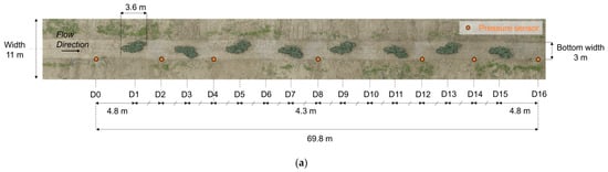
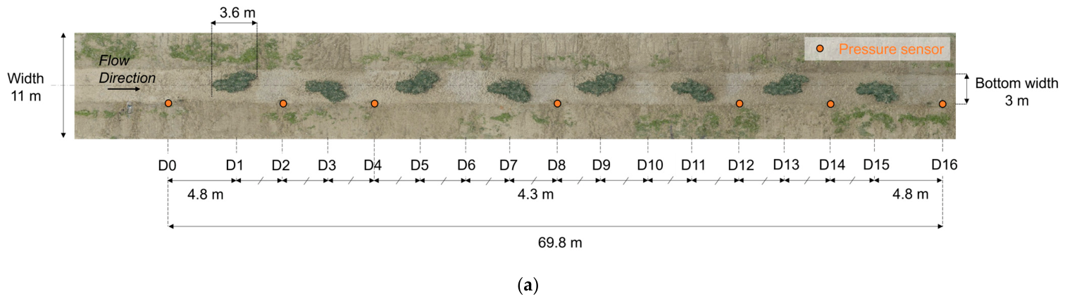
The reach-scale dataset reported by Ji et al. [26] provided the experimental basis for this study. The experiments were conducted at the River Experiment Center of the Korea Institute of Civil Engineering and Building Technology in South Korea, in a straight trapezoidal channel 69.8 m in length, with a bed slope of 1/800, bottom and top widths of 3 and 11 m, respectively, and a bank slope of 1:2 (V:H). The bed consisted of movable sand with a median grain size (d₅₀) of 1.06 mm, whereas the banks consisted of bare soil.

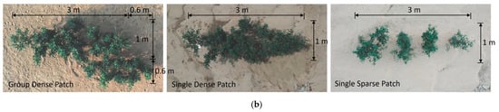
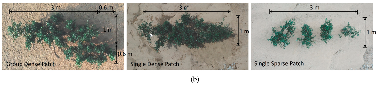
Eight artificial willow patches designed to mimic natural vegetation were installed to simulate partly vegetated channel conditions. The patch layouts were based on field observations of willow patches in the Naesungcheon Stream, a tributary of the Nakdong River. Three vegetation layouts were tested by varying patch distribution and density (Figure 1): group-dense (GD) patches comprising 23 trees arranged in clusters, single-dense (SD) patches comprising 15 trees, and single-sparse (SS) patches comprising eight trees. In each layout, eight patches were placed at regular longitudinal intervals of 8.6 m, creating partly vegetated conditions with substantial non-vegetated zones between successive patches.

Figure 1. Plan views of (a) the large-scale experimental channel layout, adapted from Ryu et al. [21], and (b) the vegetation patch layouts: group-dense (23 trees), single-dense (15 trees), and single-sparse (8 trees). Photographs in (b) were taken by the authors during the experiments described in Ji et al. [26].

Water surface levels were recorded using high-accuracy pressure sensors (accuracy, 0.05% of full scale; resolution, 0.01% of full scale, corresponding to a water level uncertainty of approximately ±2 mm) and were used as the primary reference for validation. Six experimental cases were selected to represent different combinations of vegetation layouts and densities under both low- and high-flow conditions, with discharges ranging from approximately 1.47 to 2.81 m³/s (Table 1). All selected cases involved emergent vegetation, with the water depth remaining below vegetation height. Case GDL1-1 was selected for the group-dense, low-flow condition because Ji et al. [26] identified it as a repeat run with consistent measurements. The case nomenclature indicates patch distribution (grouped or single), patch density (dense or sparse), and flow condition (high or low flow).

Table 1. Reach-scale hydraulic conditions and experimental results used for numerical modeling (based on the experimental dataset reported by Ji et al. [26]).

No.	Case	Q (m3/s)	HD16 (El.m)	h (m)	Um (m/s)	AD2 (m2)	AD14 (m2)	RD2 (m)	RD14 (m)	Sw (m/m)	Sf (m/m)	fbulk
1	GDH	2.805	98.768	0.86	0.623	4.624	4.388	0.675	0.625	0.00130	0.00126	0.165
2	GDL1-1	1.496	98.609	0.68	0.439	3.484	3.336	0.567	0.516	0.00079	0.00078	0.172
3	SDH	2.748	98.782	0.86	0.604	4.600	4.505	0.665	0.632	0.00079	0.00078	0.109
4	SDL	1.466	98.600	0.66	0.437	3.371	3.332	0.545	0.508	0.00043	0.00042	0.091
5	SSH	2.712	98.782	0.90	0.647	4.185	4.198	0.633	0.609	0.00068	0.00068	0.079
6	SSL	1.543	98.612	0.71	0.495	3.099	3.134	0.526	0.508	0.00041	0.00041	0.068

Note: In each case name, the first letter indicates patch distribution (grouped/single), the second indicates patch density (dense/sparse), and the third indicates the flow condition (high/low). See Ji et al. [26] for further details. H_D16 = the measured water surface level at downstream sensor D16, used as the downstream boundary condition; h = flow depth; U_m = the reach-scale mean velocity, equivalent to U_o in Equation (1); A and R with the subscripts D2 and D14 = the flow areas and hydraulic radii at sensors D2 and D14, respectively; S_w = the water surface slope; S_f = the friction slope calculated using Equation (2); f_bulk = the bulk Darcy–Weisbach friction factor.

2.2. Flow Resistance in Partly Vegetated Channels

Flow resistance governs the rate at which flow energy is dissipated along a channel and is influenced by bed material, bedforms, slope, cross-sectional geometry, and obstructions such as vegetation. Hydraulic resistance is commonly expressed using three interrelated empirical coefficients, namely, Manning’s n, the Chézy coefficient C, and the Darcy–Weisbach friction factor f, all of which are related through the hydraulic radius R and gravitational acceleration g:

$$C=U_o/{\left(R{S}_f\right)}^{1/2}={\left(8g/f\right)}^{1/2}=R^{1/6}/n$$

(1)

where U_o is the cross-sectionally averaged velocity (identical to the reach-scale mean velocity U_m in Table 1), and S_f is the friction slope. Manning’s n is widely used in practice because of its dimensional convenience. Accurate estimation of resistance is critical because it directly affects simulated water surface levels and velocity distributions. Because S_f cannot be measured directly, it was estimated from the measured water surface slope S_w using the following energy equation [10]:

$$S_f=S_w+\left(Q^2/2\mathit{gl}\right)\left(1/A_A^2-1/A_B^2\right)$$

(2)

where l is the distance between the two cross-sections, and A_A and A_B are the flow areas at the upstream (D2) and downstream (D14) cross-sections, respectively. The bulk Darcy–Weisbach friction factor is then obtained from $f=8\mathit{gR}{S}_f/U_m^2$, with U_m representing the reach-scale mean velocity (Table 1).

In a vegetated channel, the total resistance arises from two physically distinct sources: bed friction along the channel bed and drag exerted by vegetation elements on the flow [3]. Combining these two components is central to parameterizing vegetation resistance. Under steady, uniform flow, the total boundary shear stress can be expressed as the sum of its bed- and vegetation-related components:

τ_total = τ_bed + τ_veg

(3)

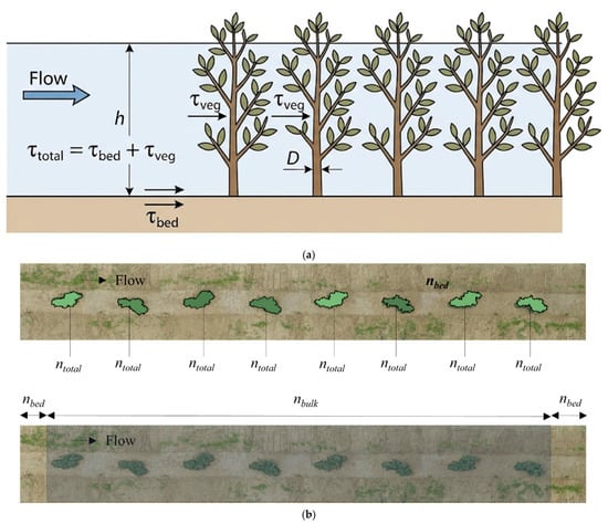
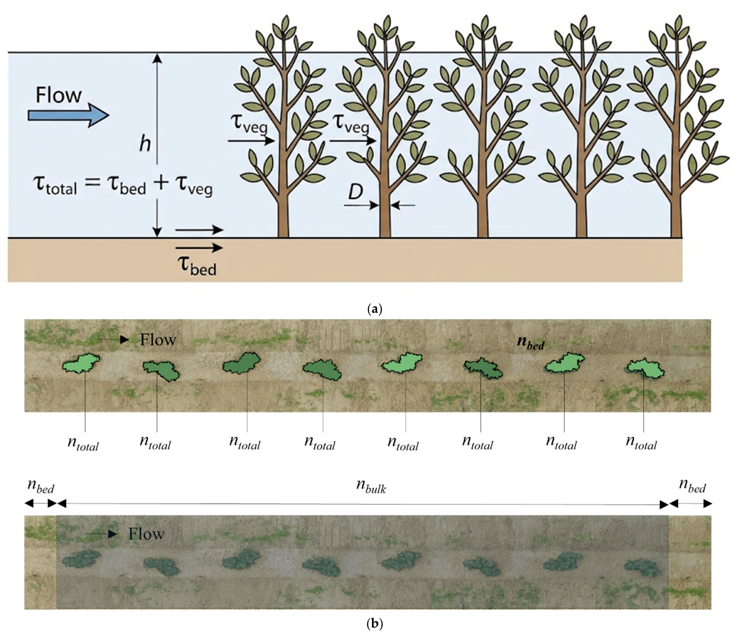
By applying the same linear superposition to the Darcy–Weisbach friction factor, Baptist et al. [15] expressed the total factor as f_total = f_bed + f_veg (Figure 2a).

Figure 2. Resistance representations: (a) conceptual decomposition of total resistance into bed friction (τ_bed) and vegetation drag (τ_veg) based on Baptist et al. [15]; and (b) representation of Manning’s n using spatially varying roughness layers under the distributed approach (n_bed and n_total) and a uniform bulk approach (n_bulk).

This additive decomposition applies to f but does not apply directly to Manning’s n. Because n is related nonlinearly to the Darcy–Weisbach friction factor through Equation (1), the corresponding roughness coefficients are combined quadratically rather than linearly:

$${n_{\mathit{total}}}^2={n_{\mathit{bed}}}^2+{n_{\mathit{veg}}}^2$$

(4)

This distinction is important in practice because simply adding the bed- and vegetation-related roughness values to obtain vegetated roughness would overstate the combined resistance. By combining the bed friction and vegetation drag contributions, Baptist et al. [15] expressed the representative resistance of a vegetated zone in terms of an equivalent Chézy coefficient as follows:

$$C_r=1/\sqrt{\left(1/C_b^2+C_D\lambda /2g\right)}$$

(5)

where C_b is the Chézy coefficient for the bare bed, C_r is the equivalent Chézy coefficient of the vegetated zone, C_D is the vegetation drag coefficient, and λ is the vegetation frontal area per unit ground area. For idealized rigid cylinders, λ = mDh, where m denotes the number of stems per unit bed area, D is the stem diameter, and h is the flow depth. The equivalent Chézy coefficient in Equation (5) is then converted into the total roughness n_total using Equation (1); the resulting value is assigned to the vegetated zones in the distributed approach described below. In this conversion, the hydraulic radius was taken as the case-specific reach-averaged value between cross-sections D2 and D14 for each case (Table 1). Equation (4) follows from applying the additive stress decomposition of Equation (3) at a common flow depth such that both components refer to the same hydraulic radius; it therefore represents the combination rule implied by the Darcy–Weisbach superposition rather than an additional empirical assumption.

The willow patches used in this study, however, consisted of multibranched, foliated woody plants whose forms differed substantially from the idealized cylindrical geometry. Representing them as simple cylinders would underestimate the frontal area presented to the flow and, consequently, underestimate the vegetation-induced resistance. The momentum-balance framework in Equations (3)–(5) does not prescribe a particular vegetation geometry; it requires only an appropriate frontal-area parameter, λ. Following Ji et al. [26], the cylindrical frontal-area term was replaced by the submerged frontal-projected stem area A_S, which includes the main stem, branches, and twigs, such that λ = mA_S. This modification preserves the underlying physical basis of the Baptist et al. [15] formulation while extending its applicability to complex, naturally shaped woody vegetation. Because A_S includes only the submerged portions of the stems, branches, and twigs, it was determined separately for each case according to the corresponding flow depth. The stem densities and frontal-projected areas for each vegetation layout were taken directly from the measurements reported by Ji et al. [26].

2.3. Distributed and Bulk Roughness Representations

The representation of resistance in a 2D model depends on how the sources of resistance are represented in relation to the spatial distribution of vegetation. When vegetation occupies only part of a cross-section, resistance is spatially nonuniform; it is dominated by vegetation drag within vegetated patch zones and by bed friction in the surrounding open-flow areas. This spatial heterogeneity can be represented using two distinct resistance parameterization approaches (Figure 2b). These approaches mirror the classical distinction between subdivided and lumped resistance representations and form the basis of the two simulation strategies compared in this study.

The first approach, referred to as the distributed or patch-scale approach, explicitly represents this heterogeneity. The momentum-based total roughness n_total, calculated using Equations (4) and (5), is assigned to the vegetated patch zones, whereas bare-bed roughness n_bed is assigned to the surrounding non-vegetated areas. Thus, the spatial variation in resistance is represented on a cell-by-cell basis across the model domain. This approach is the depth-averaged analog of the divided-channel treatment, in which each subregion is assigned a distinct resistance value. In this approach, C_D serves as a key free parameter. It was initially set to 1.5, consistent with values recommended for emergent woody vegetation [21,26], and was then varied between 0.25 and 3.0 to represent low- and high-drag conditions and evaluate the sensitivity of the resulting roughness values n_total. These three settings define the distributed scenarios A1 (C_D = 0.25), A2 (C_D = 1.5), and A3 (C_D = 3.0), with the corresponding roughness values listed in Table 2.

Table 2. Bulk and total roughness coefficients (n) used in numerical modeling and the corresponding simulation scenarios. Simulation A applied the spatially distributed (patch-scale) approach, with n_total assigned to vegetated zones; the scenarios A1, A2, and A3 correspond to C_D values of 0.25, 1.5, and 3.0, respectively. Simulation B applied the uniform bulk approach with n_bulk assigned uniformly throughout the reach.

Case	Scenario	Approach (CD)	nbed	ntotal	nbulk
GDH	A1	Distributed (CD = 0.25)	0.019	0.061	-
	A2	Distributed (CD = 1.5)	0.019	0.142	-
	A3	Distributed (CD = 3.0)	0.019	0.200	-
	B	Bulk	0.019	-	0.043
GDL1-1	A1	Distributed (CD = 0.25)	0.020	0.055	-
	A2	Distributed (CD = 1.5)	0.020	0.126	-
	A3	Distributed (CD = 3.0)	0.020	0.177	-
	B	Bulk	0.020	-	0.042
SDH	A1	Distributed (CD = 0.25)	0.019	0.060	-
	A2	Distributed (CD = 1.5)	0.019	0.140	-
	A3	Distributed (CD = 3.0)	0.019	0.197	-
	B	Bulk	0.019	-	0.035
SDL	A1	Distributed (CD = 0.25)	0.020	0.053	-
	A2	Distributed (CD = 1.5)	0.020	0.123	-
	A3	Distributed (CD = 3.0)	0.020	0.172	-
	B	Bulk	0.020	-	0.031
SSH	A1	Distributed (CD = 0.25)	0.019	0.057	-
	A2	Distributed (CD = 1.5)	0.019	0.134	-
	A3	Distributed (CD = 3.0)	0.019	0.188	-
	B	Bulk	0.019	-	0.029
SSL	A1	Distributed (CD = 0.25)	0.020	0.053	-
	A2	Distributed (CD = 1.5)	0.020	0.121	-
	A3	Distributed (CD = 3.0)	0.020	0.170	-
	B	Bulk	0.020	-	0.026

Note: n_bed = bed roughness for non-vegetated conditions; n_total = combined bed friction and vegetation drag roughness in vegetated zones, calculated using the formulation of Baptist et al. [15]; n_bulk = a single reach-integrated roughness coefficient. Scenarios A1–A3 represent the distributed approach using different C_D values, whereas scenario B represents the bulk approach.

The second approach, referred to as the bulk or reach-integrated approach, deliberately does not resolve the spatial variability of resistance. It represents the combined effects of bed friction and vegetation drag across the entire partly vegetated reach using a single coefficient, n_bulk, which is applied uniformly throughout the computational domain, without distinguishing between vegetated and non-vegetated zones. This approach is the depth-averaged 2D analog of the single-channel or lumped-conveyance treatment. Its practical advantage is that n_bulk can be derived directly from measured reach-scale hydraulic quantities using Equations (1) and (2), without requiring detailed information on vegetation geometry or drag characteristics. It must be emphasized, however, that because n_bulk is back-calculated from water surface slopes measured in the same experiments used subsequently for validation, scenario B does not constitute an independent prediction; rather, it provides an observationally anchored benchmark representing the best performance attainable using a spatially uniform coefficient. The comparison between scenarios A and B is therefore interpreted throughout this paper as a contrast between a predictive, physically based resistance parameterization and a data-anchored reference, rather than as a comparison of two methods with equivalent predictive independence. The bulk approach is designated as scenario B (bulk). Thus, the distinction between the two approaches is not only numerical but also conceptual. Distributed scenarios A1–A3 preserve the internal structure of the resistance field but require information on vegetation properties and an assumed drag coefficient, whereas bulk scenario B replaces this spatial structure with a single, observationally derived coefficient. This study therefore examines which of these trade-offs is more appropriate in a 2D model and whether this choice depends on patch arrangement.

Three coefficients were estimated from the experimental measurements reported by Ji et al. [26] and are summarized in Table 2. The bed coefficient n_bed represents flow resistance in the absence of vegetation and was obtained from baseline runs conducted without patches. The vegetation component n_veg was not applied independently; instead, it was used solely as an intermediate quantity in calculating n_total using Equation (4). The bulk coefficient n_bulk represents the reach-integrated flow resistance of the partly vegetated reach. Throughout the remainder of this paper, the distributed scenarios are denoted as A1–A3 according to the specified drag coefficient value, and the bulk scenario is denoted as B, consistent with Table 2.

2.4. HEC-RAS 2D and Model Setup

Simulations were performed using HEC-RAS 2D (version 6.5) [27], which solves the depth-averaged shallow-water equations using the finite-volume method on a computational mesh. This framework is appropriate when horizontal flow variations dominate and vertical gradients are small, as is consistent with the shallow, fully emergent conditions in all experimental cases. The diffusion wave approximation was adopted because it is suitable for the subcritical, gradually varying flow conditions in the experimental channel. Froude numbers computed from the reach-scale mean velocities and flow depths reported in Table 1 ranged from approximately 0.17 to 0.22, and the measured water surface profiles exhibited no abrupt transitions, thereby supporting this choice. The neglected momentum terms are also quantitatively small under these conditions: the advective terms scale with the square of the Froude number (Fr² ≈ 0.03–0.05), and the change in velocity head along the validation reach, calculated from the measured flow areas in Table 1, is at most 2.1 mm (GDH) and less than 1 mm in all other cases—about an order of magnitude smaller than the approximately 19–34 mm separation between the A3 and B mean water level biases in the grouped cases on which the conclusions rest. Because both parameterizations were solved using the identical scheme, mesh, and terrain, any residual approximation error is common to both and therefore largely cancels out in their comparison. However, this formulation neglects the inertial and advective momentum terms; therefore, inertia-dependent features such as wake recirculation behind patches cannot be explicitly reproduced. The simulated velocity fields primarily reflect the balance between the water surface gradient and the assigned resistance rather than the fully resolved patch-scale hydrodynamics. The implications of this approximation for interpreting the results are discussed in Section 4.1 and Section 4.3. The lateral-inflow and surface stress terms were neglected because the simulations represented closed-flume experimental conditions without lateral inflow or wind forcing. A fixed computational time step, selected to satisfy the Courant condition, was used for all simulations. Turbulent momentum exchange terms, including those represented through eddy viscosity, are not active in the diffusion wave formulation. Bed shear stress was evaluated using Manning’s equation, thereby linking the model formulation to the flow resistance parameterization described in Section 2.2. Each case was simulated under constant boundary conditions until a stationary water surface profile was attained at every sensor location, which was used as the convergence criterion, with the fixed time step satisfying the Courant condition throughout. The vegetated-zone roughness polygons coincided exactly with the digitized patch perimeters, whereas the remaining wetted domain was assigned the bed roughness, and the bulk coefficient was derived from the reach-scale friction slope between cross-sections D2 and D14 obtained from Equations (1) and (2) and the mean hydraulic radius of the bounding cross-sections (Table 1).

Hydraulic boundary conditions were obtained directly from Ji et al. [26]. The measured discharge was specified at the upstream boundary, and the measured water surface level at sensor D16 was prescribed as the downstream boundary condition. Sensor D16 was therefore excluded from validation to avoid circularity, and D0 was excluded because of its proximity to the inlet, leaving sensors D2, D4, D8, D12, and D14 as the validation locations. Stations D6 and D10 were not instrumented for water-level measurement in the original experiments; pressure sensors were installed at only seven cross-sections (D0, D2, D4, D8, D12, D14, and D16) [26], so the validation set follows directly from the available instrumentation. As the downstream water level was prescribed at D16, simulation errors are expected to diminish toward D14; therefore, the upstream sensors carry the greatest discriminatory weight in the evaluation. For completeness, errors at D0 are reported in Table 3 and Table 4, but they were excluded from all error statistics. The bed terrain was reconstructed from high-density point-cloud data collected through 3D scanning during the experiments. The data were filtered to remove noise, spikes, and non-bed features, particularly vegetation, and were then converted into raster digital elevation models, with a separate dataset used for each vegetation layout.

Table 3. Measured water surface levels (El.m) and Simulation A errors (simulated − measured, m) for the spatially distributed approach using the Baptist et al. [15] formulation with different drag coefficients (C_D).

Case	Method		Measured WSL (El.m) and Simulation Error (Simulated − Measured, m)
			D0	D2	D4	D8	D12	D14
GDH	Measured (El.m)		98.859	98.847	98.830	98.814	98.791	98.780
	Simulation Error (m)	A1	−0.061	−0.053	−0.040	−0.031	−0.015	−0.008
		A2	−0.055	−0.048	−0.036	−0.028	−0.014	−0.007
		A3	−0.052	−0.046	−0.034	−0.027	−0.016	−0.007
GDL1-1	Measured (El.m)		98.663	98.654	98.645	98.634	98.621	98.613
	Simulation Error (m)	A1	−0.034	−0.028	−0.022	−0.015	−0.007	−0.002
		A2	−0.030	−0.024	−0.019	−0.013	−0.006	−0.001
		A3	−0.028	−0.023	−0.017	−0.012	−0.006	−0.001
SDH	Measured (El.m)		98.837	98.832	98.823	98.814	98.801	98.791
	Simulation Error (m)	A1	−0.031	−0.029	−0.023	−0.020	−0.013	−0.006
		A2	−0.028	−0.027	−0.021	−0.019	−0.012	−0.005
		A3	−0.027	−0.026	−0.021	−0.018	−0.012	−0.005
SDL	Measured (El.m)		98.629	98.626	98.621	98.617	98.608	98.604
	Simulation Error (m)	A1	−0.010	−0.009	−0.007	−0.007	−0.004	−0.001
		A2	−0.008	−0.008	−0.006	−0.006	−0.003	−0.001
		A3	−0.007	−0.007	−0.005	−0.006	−0.003	−0.001
SSH	Measured (El.m)		98.828	98.826	98.819	98.810	98.799	98.791
	Simulation Error (m)	A1	−0.025	−0.026	−0.022	−0.018	−0.011	−0.006
		A2	−0.023	−0.024	−0.021	−0.017	−0.011	−0.006
		A3	−0.023	−0.024	−0.020	−0.017	−0.011	−0.006
SSL	Measured (El.m)		98.640	98.637	98.632	98.628	98.621	98.616
	Simulation Error (m)	A1	−0.011	−0.010	−0.007	−0.007	−0.004	−0.002
		A2	−0.009	−0.008	−0.006	−0.006	−0.004	−0.001
		A3	−0.008	−0.008	−0.005	−0.006	−0.004	−0.001

Table 4. Measured water surface levels (El.m) and Simulation B errors (simulated − measured, m) for the uniform bulk approach (Simulation B).

Case	Method	D0	D2	D4	D8	D12	D14
GDH	Measured (El.m)	98.859	98.847	98.830	98.814	98.791	98.780
	Simulation Error (m)	+0.010	+0.009	+0.015	+0.008	+0.007	+0.003
GDL1-1	Measured (El.m)	98.663	98.654	98.645	98.634	98.621	98.613
	Simulation Error (m)	+0.008	+0.009	+0.010	+0.008	+0.005	+0.005
SDH	Measured (El.m)	98.837	98.832	98.823	98.814	98.801	98.791
	Simulation Error (m)	+0.009	+0.005	+0.006	+0.001	−0.002	0.000
SDL	Measured (El.m)	98.629	98.626	98.621	98.617	98.608	98.604
	Simulation Error (m)	+0.008	+0.006	+0.007	+0.002	+0.002	+0.002
SSH	Measured (El.m)	98.828	98.826	98.819	98.810	98.799	98.791
	Simulation Error (m)	−0.005	−0.008	−0.007	−0.007	−0.006	−0.003
SSL	Measured (El.m)	98.640	98.637	98.632	98.628	98.621	98.616
	Simulation Error (m)	−0.002	−0.002	−0.001	−0.003	−0.002	0.000

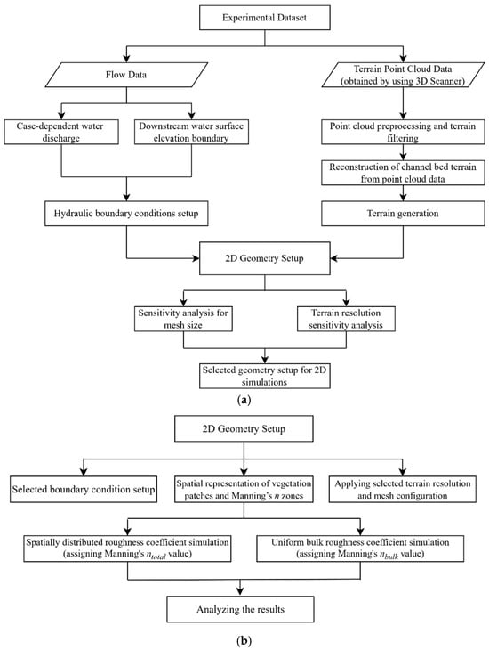
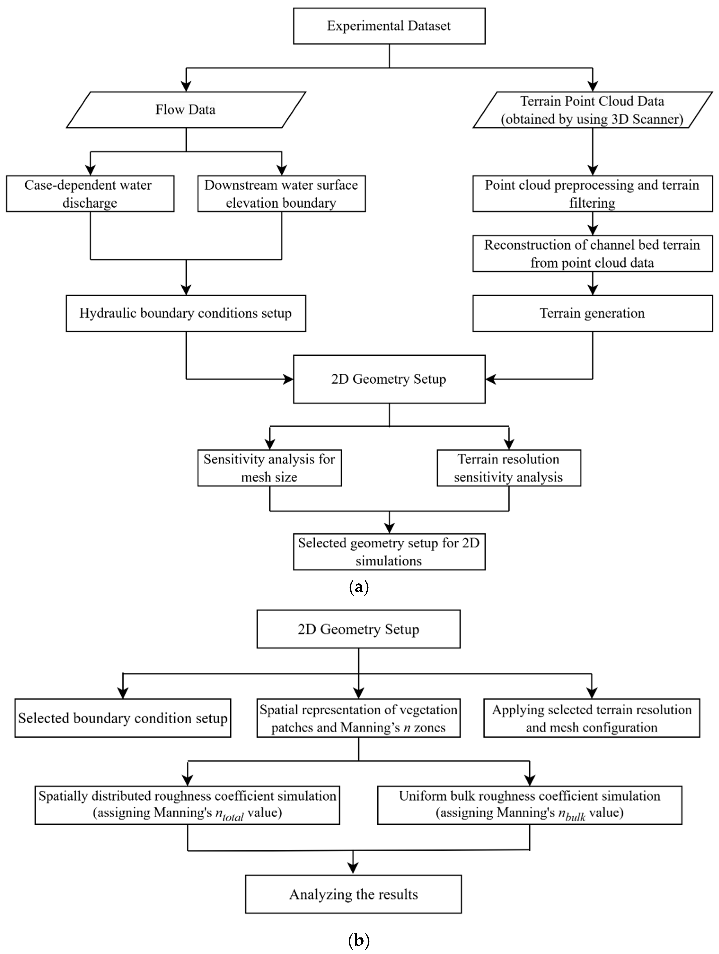
The terrain and computational mesh settings were determined after a preliminary assessment. A raster terrain resolution of 0.001 m was adopted to represent the channel bathymetry and vegetation patch boundaries in detail, and a computational mesh size of 0.25 m was selected to balance spatial resolution with numerical stability. In the preliminary assessment, coarser and finer meshes with sizes of 0.5 and 0.1 m, respectively, were also tested under identical boundary conditions. Between the two finest meshes (0.25 and 0.1 m), the simulated water surface levels differed by less than 1 mm in the single-patch cases and by up to approximately 10 mm in the grouped-dense cases. As the same mesh was used for every case and scenario, this residual sensitivity affects all roughness parameterizations in the same manner and does not alter their comparison. This band of mesh-induced differences is smaller than the 19–34 mm separation between the opposing distributed and bulk biases reported in Section 3.3, indicating that the direction-of-bias finding is unlikely to be an artifact of the spatial discretization. The selected settings produced stable and consistent results and were used in all simulations (Figure 3). These optimal values reflect the scale of the experimental flume used in this study, and an equivalent sensitivity assessment would be required to establish appropriate resolution and mesh settings for channels at a different scale. As terrain resolution and mesh design are known to influence 2D hydrodynamic predictions [28,29], this configuration was maintained consistently across all cases and scenarios to isolate the effects of roughness parameterization. Vegetation effects were incorporated through a land cover layer that spatially assigned values of Manning’s n rather than through the explicit representation of vegetation as drag. The two parameterizations were then evaluated under identical geometric and boundary conditions. Distributed scenarios A1–A3 applied n_total within the vegetated zones and n_bed elsewhere, with the patch boundaries digitized over the terrain, whereas bulk scenario B applied the uniform bulk coefficient n_bulk throughout the computational domain.

Figure 3. Two-dimensional modeling workflow for the partly vegetated channel: (a) initial geometry preparation, including terrain and mesh setup and sensitivity analysis; and (b) the hydrodynamic modeling procedure using the two resistance approaches.

3. Results and Analysis

3.1. Distributed Approach: Scenarios A1–A3

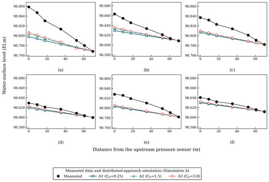
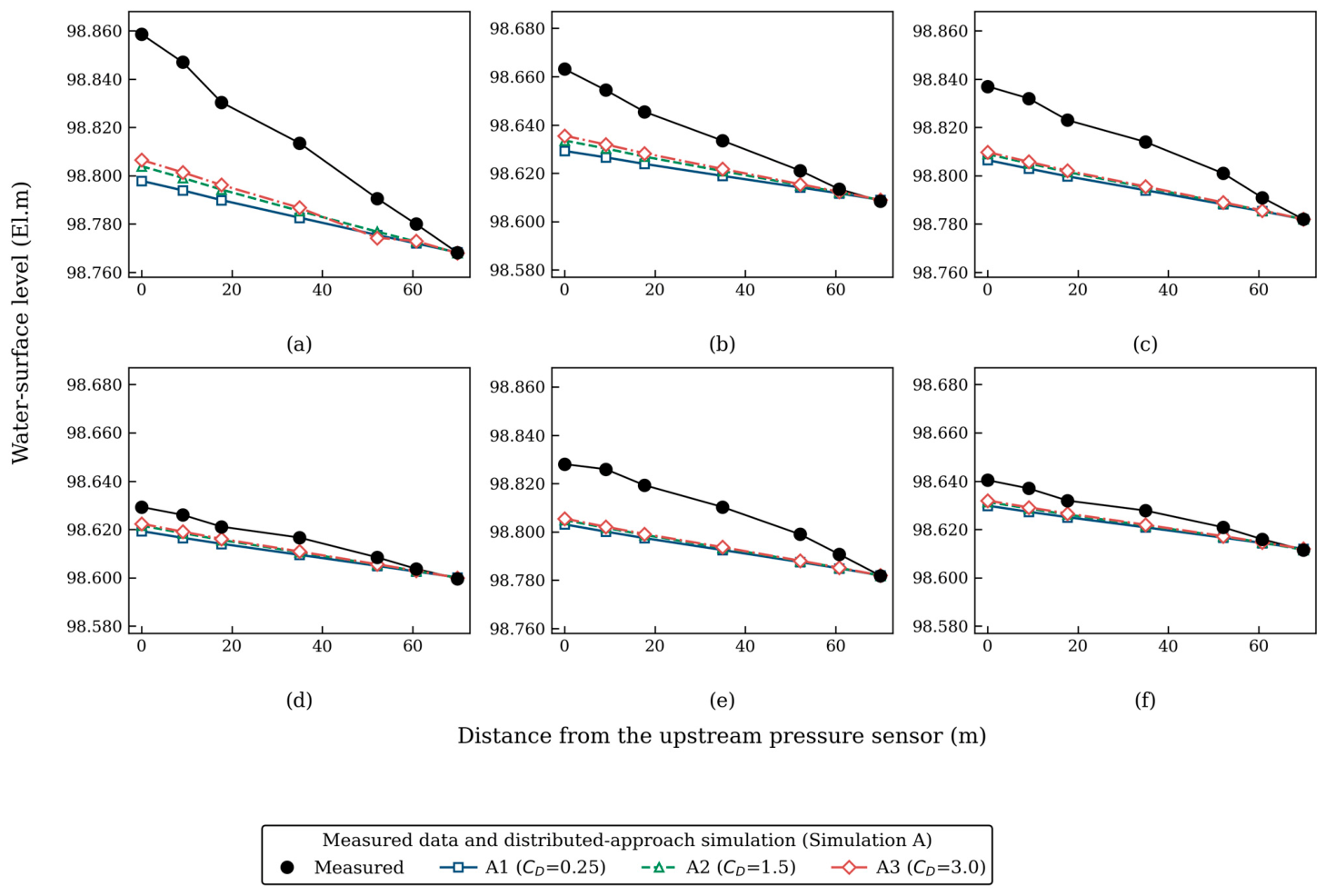
Across all six cases, the distributed approach (scenarios A1–A3) consistently underestimated the measured water surface levels (WSLs), and the errors reported in Table 3 were predominantly negative. Throughout this paper, the tabulated errors in Table 3 and Table 4 are rounded to 0.001 m, whereas the MAE values in Table 5 are computed from the unrounded output of the same final simulation set; therefore, mean values recomputed from the rounded table entries may differ from those in Table 5 by a few tenths of a millimeter. However, the sensitivity to the drag coefficient differed markedly among the patch configurations (Figure 4).

Table 5. Summary of model performance across all cases and approaches, expressed as the mean absolute error (MAE, mm) of simulated water surface levels at the validation cross-sections (D2–D14). Cell shading indicates the error magnitude. Simulation A used the spatially distributed approach based on the formulation of Baptist et al. [15], with C_D values of 0.25, 1.5, and 3.0 for scenarios A1, A2, and A3, respectively; Simulation B used the uniform bulk roughness coefficient approach.

Case	A1 (CD = 0.25)	A2 (CD = 1.5)	A3 (CD = 3.0)	B (Bulk)
GDH	29.5	26.6	26.0	8.4
GDL1-1	14.8	12.6	11.8	7.5
SDH	18.2	16.8	16.4	2.9
SDL	5.6	4.8	4.4	3.7
SSH	16.6	15.8	15.6	6.2
SSL	6.0	5.0	4.8	1.6

Figure 4. Longitudinal water surface profiles (El.m) obtained using the distributed approach (Simulation A) and the Baptist et al. [15] formulation under scenarios A1–A3 (C_D = 0.25, 1.5, and 3.0, respectively): (a) GDH; (b) GDL1-1; (c) SDH; (d) SDL; (e) SSH; and (f) SSL.

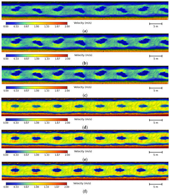
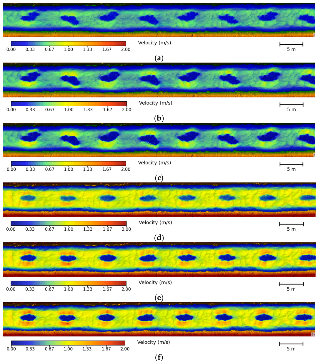
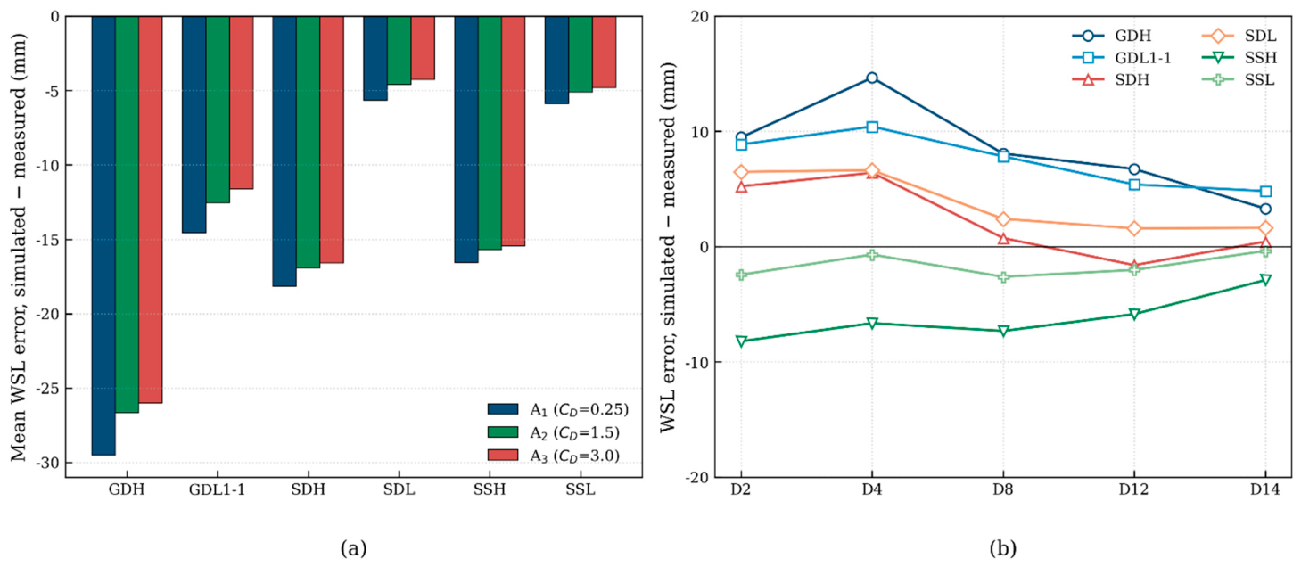
In the grouped-dense cases, increasing C_D from the value used in A1 to the value used in A3 progressively reduced the underestimation. For GDH, the mean absolute error across the validation sensors decreased from approximately 0.030 m in A1 to 0.026 m in A3, whereas for GDL1-1, the MAE decreased to a minimum of approximately 0.012 m (Table 5). However, none of the scenarios achieved close agreement with the measurements, and the larger errors under higher discharge conditions indicated that flow magnitude amplified the underestimation in the grouped configurations. The velocity fields showed that the low-velocity zones within the patches expanded from A1 to A3 (Figure 5), confirming that the formulation represented increased resistance within the patches as intended. As the diffusion wave solver derives velocities diagnostically from the water surface gradient and the assigned roughness, these velocity fields should be interpreted as indicating the spatial allocation of resistance rather than representing fully resolved patch-scale flow structures, such as wakes.

Figure 5. Representative velocity distribution maps for scenarios A1–A3 (C_D = 0.25, 1.5, and 3.0): (a–c) grouped case GDL1-1 and (d–f) the single-patch case SDL.

In contrast, all single-patch cases showed negligible changes across scenarios A1–A3. The mean errors remained at approximately −0.018 to −0.015 m for the high-flow cases (SDH and SSH) and between −0.006 and −0.004 m for the low-flow cases (SDL and SSL), with changes of no more than 0.001–0.002 m among scenarios (Table 5; Figure 6a). The spatial extent of the low-velocity zones around the isolated patches likewise remained essentially unchanged (Figure 5). Thus, the magnitude of underestimation in the single-patch configurations was influenced more by discharge than by the drag coefficient, and adjusting C_D alone did not meaningfully improve the hydraulic response. The sparse and dense single-patch cases produced comparable error patterns, indicating that density had little influence within the single-patch arrangement and suggesting that patch arrangement was a more influential factor. However, arrangement and density were partially confounded in the experimental design because the grouped layout was also the densest configuration, and no grouped-sparse case was available. Across all configurations, the low-flow cases produced consistently smaller errors than their high-flow counterparts (Figure 6a).

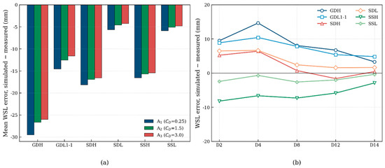
Figure 6. Analysis of water-surface-level errors: (a) mean water-surface-level error (simulated − measured), averaged over sensors D2, D4, D8, D12, and D14, for all cases under the distributed approach in scenarios A₁–A₃; and (b) longitudinal error distributions for all cases under the bulk approach.

3.2. Bulk Approach: Scenario B

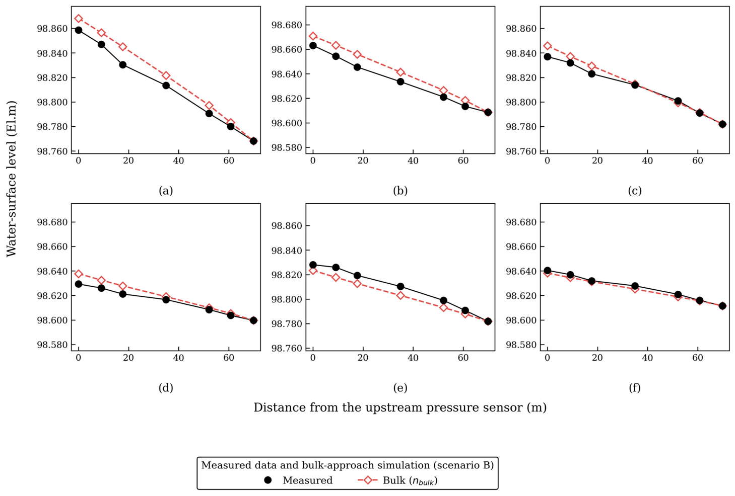
Applying a single coefficient throughout the domain produced overall closer WSL predictions, although performance remained clearly patch configuration dependent (Table 4; Figure 7).

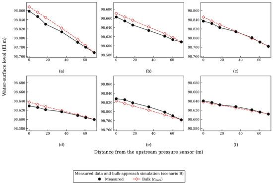
Figure 7. Longitudinal water surface profiles from the bulk approach (scenario B, n_bulk) compared with the measured data for all six cases: (a) GDH, (b) GDL1-1, (c) SDH, (d) SDL, (e) SSH, and (f) SSL.

In contrast to the distributed approach, the bulk approach consistently overpredicted WSLs in the grouped-dense cases. The errors reported in Table 4 were positive for GDH and GDL1-1, and the corresponding mean absolute errors (MAEs) were approximately 8.4 mm and 7.5 mm, respectively, with the higher-discharge case showing a greater deviation. Among the single-patch cases, the dense cases (SDH and SDL) showed slight overprediction that decreased downstream, with MAEs of approximately 2.9 mm and 3.7 mm, respectively. In contrast, the sparse cases (SSH and SSL) showed slight underestimation of the measurements, with MAEs of approximately 6.2 mm and 1.6 mm, respectively. SSL showed the closest agreement among all cases. The low-flow cases showed lower MAEs than their high-flow counterparts for the grouped-dense and single-sparse configurations, but not for the single-dense configuration, indicating that the bulk approach was most reliable when vegetation-induced resistance constituted a smaller proportion of the total resistance.

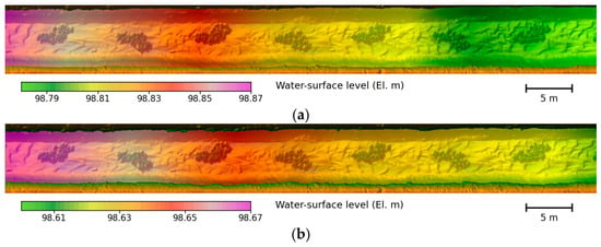
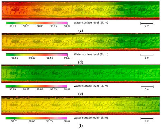
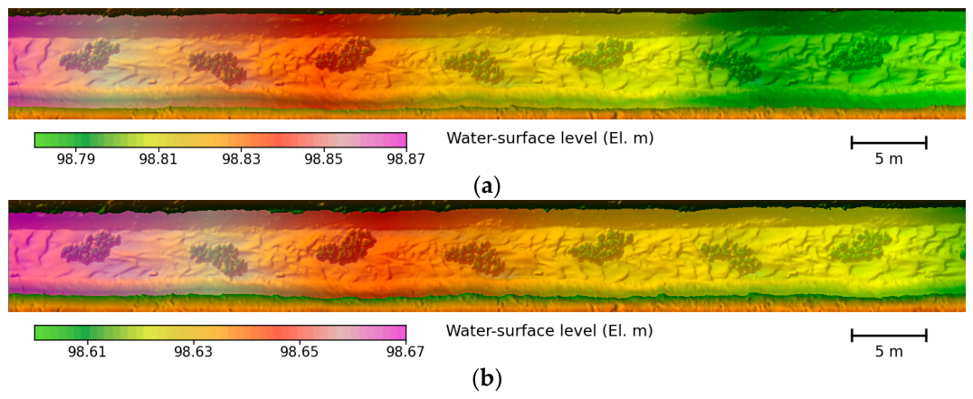
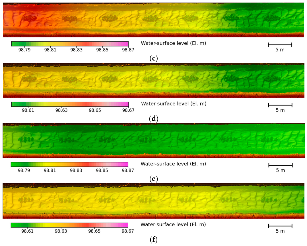
The plan-view water level maps obtained using n_bulk were laterally uniform and showed no distinct spatial variations at the patch locations (Figure 8). This result was consistent with the spatially uniform resistance assumption, which reproduced the reach-scale energy gradient but could not capture local flow contrasts. Thus, the performance of n_bulk varied systematically according to patch arrangement, vegetation density, and flow conditions rather than remaining consistent across cases.

Figure 8. Plan-view maps of water surface levels obtained using the bulk approach (scenario B, n_bulk) for all six cases: (a) GDH, (b) GDL1-1, (c) SDH, (d) SDL, (e) SSH, and (f) SSL.

3.3. Synthesis Across All Cases and Approaches

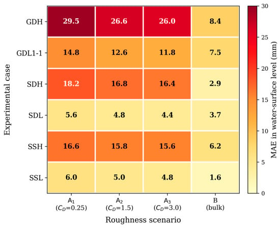
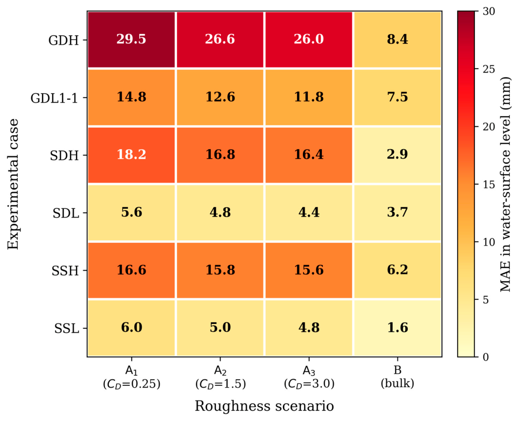
All six experimental cases (GDH, GDL1-1, SDH, SDL, SSH, and SSL) were simulated under all roughness scenarios. To provide a compact comparison of model performance, the MAE of the simulated WSLs at the validation cross-sections (D2–D14) is summarized for all cases and scenarios in Table 5 and shown as a heat map in Figure 9.

Figure 9. Heat map summary of the mean absolute error (MAE, mm) across all six cases and four roughness scenarios (A1–A3 distributed scenarios, and B bulk scenario) over D2–D14; corresponding values are presented in Table 5.

This synthesis clearly demonstrates the dependence of model performance on patch configuration. For the grouped-dense cases, bulk scenario B produced markedly lower errors than the distributed scenarios A1–A3, with MAEs of 8.4 mm for GDH and 7.5 mm for GDL1-1. For GDH, the distributed-scenario errors ranged from 26.0 to 29.5 mm, and increasing C_D reduced these errors only modestly. For the single-patch cases, the errors were generally smaller, ranging from 1.6 to 6.2 mm for the bulk approach and from 4.4 to 18.2 mm for the distributed approach, and showed little sensitivity to C_D. The lowest errors overall were obtained using the bulk approach for the single-patch cases: 1.6 mm for SSL, 2.9 mm for SDH, and 3.7 mm for SDL. The highest error occurred in the grouped high-flow case under the distributed approach, with an MAE of approximately 29.5 mm in GDH.

Across the complete matrix, scenario A3 consistently yielded the lowest MAE among the distributed scenarios for all six cases, although its improvement over A2 was small. The bulk coefficient approach was clearly preferable for the grouped patches and also produced lower MAEs in all single-patch cases. Notably, the two approaches produced errors in opposite directions in the grouped cases: the distributed approach underpredicted WSLs, whereas the bulk approach overpredicted them. This result is consistent with the classical finding that subdivided or divided-channel and lumped or single-channel conveyance treatments can bias predictions in opposite directions [19]. This pattern, which is shown by the signed errors in Table 3 and Table 4 and in Figure 6, is the central empirical finding of this study and provides the basis for the configuration-specific guidance discussed below. Two complementary checks further support this result. First, because the water level errors carry a single sign in nearly every case–scenario combination (Table 3 and Table 4), the absolute mean bias equals the MAE for those combinations in which all errors share the same sign, and the corresponding RMSE values exceed the MAE by less than 5 mm; therefore, the scenario ranking by MAE within each experimental case is preserved when the RMSE is used. Second, recomputing every statistic without the boundary-adjacent sensor D14 (i.e., over D2–D12) changes the MAE values by no more than 5.5 mm, does not alter any ranking or bias direction, and slightly widens the separation between the distributed and bulk biases in the grouped cases.

4. Discussion

4.1. Roughness Coefficient Response to Vegetation Patches in 2D Modeling

Both approaches showed configuration-dependent performance that differed substantially between the grouped and single-patch arrangements. Under the distributed approach, the Baptist et al. [15] formulation underestimated WSLs in all cases. In the grouped configurations, increasing C_D from A1 to A3 reduced the underestimation but did not fully eliminate it. Bypass flow along the channel margins remained elevated regardless of C_D, indicating that the formulation could not fully capture how a grouped array collectively blocked and redirected the flow. The reference value used here (A2, C_D = 1.5) was consistent with that used in the 1D analysis of Ryu et al. [21] for the same willow vegetation. However, the incomplete improvement suggests a structural rather than a purely calibration-related limitation. The form of the response supports this interpretation: for GDH, the improvement in MAE fell from 2.9 mm (A1→A2) to 0.6 mm (A2→A3) even though the drag coefficient doubled, i.e., from approximately 2.3 mm to 0.4 mm per unit of C_D. This deceleration reflects the asymptotic behavior of Equation (5): as C_D increases, in-patch velocities approach zero, the drag force C_Du² saturates, and the patch tends toward its solid-obstruction limit; therefore, the water level response shows diminishing sensitivity to CD while remaining below the measurements over the tested range. Even a linear extrapolation of the last observed rate would require C_D values near 70 to close the remaining ≈26 mm underestimation—one to two orders of magnitude beyond the range of 1–3 established for foliated willows—which confirms that the residual error is structural rather than parametric. Part of the residual underestimation may also reflect the diffusion wave approximation itself, which cannot explicitly resolve the inertial component of patch-induced resistance. Separating the contribution of the momentum approximation from that of the roughness formulation would require repeating the simulations using the full shallow-water solver; such a comparison is identified as a priority for future work. The Baptist et al. [15] formulation was developed for uniformly distributed cylindrical vegetation, whereas grouped patches can generate greater blockage and collective flow redirection, as demonstrated by Bae et al. [10].

For isolated patches, the approach was essentially insensitive to C_D across scenarios A1–A3. As isolated patches generate less blockage, flow tends to bypass them rather than being forced through a continuous array. Adjusting C_D therefore alters only the resistance within the patches, rather than the dominant bypass mechanism, making the underestimation primarily structural. Formulations that explicitly account for patch-scale blockage and lateral redistribution, such as that proposed by Bae et al. [10], may be more appropriate for isolated configurations, although their implementation within the Manning’s roughness framework in HEC-RAS 2D is beyond the scope of this study.

The bulk approach overpredicted WSLs in the grouped cases. Conceptually, n_bulk represents the reach-averaged resistance across the combined vegetated and non-vegetated zones, consistent with the manner in which it is derived. In a 1D setting, the results of Ryu et al. [21] closely matched the measurements. However, applying the same value uniformly to every 2D cell assigns vegetation-level resistance to otherwise lower-resistance non-vegetated zones, thereby overestimating the total resistance. This effect is particularly evident in the grouped-dense cases, in which vegetation accounts for a larger proportion of the reach-scale resistance. This behavior is the depth-averaged manifestation of the well-known tendency of lumped single-channel conveyance methods to misrepresent resistance when strong lateral heterogeneity is present [19]. The laterally uniform velocity fields indicate that the bulk approach captures the reach-scale energy gradient but cannot resolve local flow structure around discrete patches. It performed better in the single-patch configurations, and the very low error for SSL most likely reflects the relatively small resistance contribution of the sparse patches rather than an accurate representation of the local flow structure.

4.2. What the Two-Dimensional Framework Adds to One-Dimensional Analysis

As the same willow patch experiments were previously analyzed using a 1D model that compared bulk and composite roughness treatments [21], it is important to clarify what the present depth-averaged analysis adds and why the two approaches differ fundamentally. In a 1D framework, each cross-section is assigned a single section-averaged resistance. Distributed and bulk treatments can therefore differ only in the resistance value assigned to each section; the spatial arrangement of vegetation across the channel width cannot be represented. Once the section-averaged resistance is calibrated, the model can reproduce the measured longitudinal water surface profile. Ryu et al. [21] reported that the performance of the 1D roughness treatments depended on the vegetation configuration and flow conditions, with drag-coefficient adjustment improving the composite-method results for dense vegetation. However, these 1D results do not address the question most relevant to spatially explicit modeling: how resistance should be distributed across the width of a partly vegetated channel and whether the appropriate distribution depends on vegetation arrangement.

The 2D analysis yielded a result that a 1D model cannot produce. When resistance is resolved cell by cell, the distributed and bulk treatments differ not only in their coefficient values but also in the spatial structure of the resistance field. The two treatments produced oppositely directed errors for grouped patches: the distributed treatment underpredicted water levels by up to approximately 30 mm, whereas the bulk treatment overpredicted them by approximately 8 mm. This opposing bias is not merely a calibration artifact but rather a structural consequence of how each treatment allocates resistance across the vegetated and non-vegetated portions of the cross-section. It has no equivalent in a 1D scheme, in which lateral resistance allocation does not exist. The finding that patch arrangement, rather than vegetation density, affects which spatial allocation is reliable is therefore specific to the depth-averaged framework and could not have emerged from a section-averaged analysis. Thus, the present study does not simply extend the 1D comparison to two dimensions. Instead, it identifies a configuration-dependent direction of bias that becomes visible only when resistance is spatially distributed and directly informs resistance parameterization in 2D models of partly vegetated reaches.

A corollary of this finding is that the close agreement previously reported for the 1D model should not be interpreted as evidence that the choice of roughness representation is similarly unimportant in 2D. In contrast, simulations of a reach that is well represented by a calibrated section-averaged coefficient can be systematically biased in a 2D model depending on whether resistance is lumped or distributed, and the direction of this bias depends on the patch configuration. This distinction is particularly important because 2D models are increasingly used precisely in situations where 1D averaging is considered inadequate for resolving lateral flow redistribution around vegetation [5,24]. The present results show that moving to a 2D framework shifts the modeling challenge from the calibration of a single coefficient to the selection of an appropriate spatial allocation of resistance.

4.3. Practical Considerations for Roughness Coefficient Selection

These results provide a basis for selecting roughness parameterizations for the 2D modeling of partly vegetated channels, with the spatial arrangement of patches playing a key role. They also contribute to the broader effort to standardize the representation of vegetation and nature-based interventions in HEC-RAS, where the absence of agreed parameter selection methods has been identified as a barrier to consistent practice [4]. Under the distributed approach, drag coefficients greater than the commonly assumed value of 1.5 in scenario A2 may be more appropriate for densely foliated, multi-branched willow vegetation in grouped configurations. This interpretation is consistent with Bae et al. [10], who reported that effective drag increases with canopy density and blockage. Nevertheless, the formula could not fully represent the collective resistance of a grouped array, thereby limiting its applicability to this configuration. For isolated patches, formulations that explicitly account for patch-scale blockage and bypass flow are likely to be more suitable.

Although n_bulk produced more accurate overall predictions, its uniform application across a 2D domain is problematic because it assigns excessive resistance to non-vegetated zones. A spatially differentiated representation of resistance between vegetated and non-vegetated areas would be more physically appropriate for grouped configurations. The reliability of n_bulk also depends on its derivation from measured hydraulic data. Such data are seldom available in field applications, where the coefficient must instead be estimated from vegetation properties or indirect measurements. Its reliability under field conditions therefore requires further evaluation. Conditions comparable to those examined here occur in intermittently vegetated, sand-bed streams, in which emergent willow patches colonize a limited fraction of the active channel width. The most direct field analogue is the Naesungcheon Stream (Nakdong River basin, Republic of Korea), whose surveyed willow patch geometries were used as templates for the experimental layouts (Section 2.1); other vegetated sand-bed reaches for which patch-scale field measurements have been reported [13] represent similar settings. The present findings are therefore most directly applicable to such reaches.

This study had several limitations. The comparison between the two approaches is inherently asymmetric. The bulk coefficient was back-calculated from the measured hydraulic data obtained in the same experiments, so its low errors represent an upper bound on the performance of a spatially uniform coefficient rather than an independent prediction, whereas the distributed approach was applied predictively. A stricter test would require the cross-application of bulk coefficients across different flow conditions or their estimation from vegetation properties alone. In addition, the diffusion wave approximation omits inertial and advective momentum terms, so the reported errors combine the effects of the roughness parameterization with those of the momentum approximation. Repeating the analysis using the full shallow-water equations would help to distinguish these two effects. Some differences in mean absolute error among scenarios are also on the same order as the water level measurement uncertainty, so fine distinctions among the best-performing scenarios should be interpreted with caution.

Several additional limitations relate to the available data and the generalizability of the results. As the grouped layout was also the densest and no grouped-sparse configuration was tested, the effects of arrangement and density could not be fully separated, and the conclusion that arrangement is the dominant factor should be regarded as provisional. Validation also relied primarily on water surface levels because in-patch velocity measurements were unavailable in the reference dataset. This reduced the discriminatory power of the evaluation because both approaches could reproduce the reach-scale energy gradient despite producing different local flow structures. Direct velocity measurements would provide a more rigorous evaluation and are recommended for future studies. Velocity and wake measurements reported for comparable willow patches at the same experimental facility [13] could support such an evaluation, provided that a momentum-conserving hydrodynamic solver is employed. Model performance was also summarized primarily using the MAE, and complementary metrics could further strengthen the comparison where complete measured records are available. Finally, the results were obtained under controlled flume conditions involving simplified, uniformly spaced patch arrangements, fixed geometries, and rigid artificial vegetation. Natural vegetated channels contain irregular patch distributions, variable geometries, movable beds, and flexible vegetation that can reconfigure under flow [13]. In this respect, sediment transport, bed deformation, and bedform development were deliberately not simulated, even though the experimental bed consisted of movable sand. This choice is consistent with the validation target: the model terrain was reconstructed from 3D scans of the actual experimental bed, so the geometry—including the bedforms that developed during the runs—was represented in the 0.001 m terrain, and the bed roughness coefficient, derived from baseline runs over the same bed, implicitly accounts for both grain and form resistance. The measured water surface levels used for validation therefore correspond to this quasi-steady bed state. Coupling morphodynamics would have allowed the bed, and hence the resistance, to evolve during each simulation, thereby confounding the attribution of water level differences to the roughness parameterization that this study was designed to isolate. The configuration-dependent limitations identified here may therefore be more pronounced under field conditions, and the current formulations may require additional parameters, such as measures of patch-scale blockage, to remain reliable in practice.

5. Conclusions

This study evaluated Manning’s roughness parameterization in HEC-RAS 2D simulations of partly vegetated channels using reach-scale experimental data for grouped and isolated patch configurations reported by Ji et al. [26]. A terrain resolution of 0.001 m and a mesh size of 0.25 m were used consistently across all cases, with the terrain dataset corresponding to each vegetation layout so that differences in model performance could be attributed to roughness parameterization rather than differences in spatial discretization.

The distributed approach (scenarios A1–A3), based on the momentum-based resistance formulation of Baptist et al. [15], consistently underestimated measured water surface levels. In grouped patch configurations, it showed only a partial response to changes in the drag coefficient, with mean absolute errors (MAEs) of approximately 26–30 mm under high-flow conditions (Table 5). In isolated patch configurations, the results showed negligible sensitivity across the tested range of C_D = 0.25–3.0. This finding indicates that the error in the isolated cases was primarily structural rather than parametric because the formulation could not represent the bypass-dominated resistance mechanism. The bulk approach (scenario B) reproduced water levels more closely overall but also exhibited configuration-dependent performance. As its coefficient was back-calculated from measurements obtained in the same experiments, its performance served as an observationally anchored benchmark rather than an independent prediction. It overpredicted water levels in the grouped-dense patch configurations, with MAEs of approximately 7.5–8.4 mm, while producing generally smaller errors for isolated patches. However, it generated laterally uniform flow fields in all cases, reproducing the reach-scale energy gradient while failing to resolve local flow structures around individual patches.

Neither approach performed consistently across all configurations and model performance varied according to patch arrangement, vegetation density, and flow conditions. The synthesis of all six cases under all scenarios (Table 5) demonstrated this pattern clearly. The bulk coefficient minimized the error for grouped patches, with MAEs of approximately 7.5–8.4 mm, compared with 11.8–29.5 mm for the distributed approach. For isolated patches, the errors were generally smaller, and the bulk benchmark produced the lower MAE in all four isolated-patch cases, although its MAE advantage over A3, the best-performing distributed scenario, varied substantially with density and flow condition, from 0.7 mm (SDL) to 13.5 mm (SDH); the magnitude of the difference between the two approaches thus remained configuration-dependent. Importantly, the two approaches produced errors in opposite directions for grouped patches, demonstrating that the choice between distributed and bulk representations depends not only on coefficient calibration but also on how resistance is spatially allocated in relation to vegetation arrangement.

This opposing bias is specific to the spatially resolved 2D framework and has no counterpart in the section-averaged 1D analysis of the same reach, where resistance is represented by a single value at each cross-section [21]. The principal contribution of this study is the identification of this configuration-dependent bias. The main practical implication is that resistance parameterization in 2D models of partly vegetated channels should explicitly account for vegetation patch arrangement rather than assume that a single approach is applicable to all layouts.

These findings were obtained under controlled flume conditions with fixed geometry, fully emergent rigid vegetation, the diffusion wave approximation, and a case matrix in which patch arrangement and density were partially confounded. Further investigation is therefore required before the findings can be reliably generalized to field conditions involving variable cross-sections, movable beds, flexible vegetation, and partially submerged canopies.

References

- Hubble, T.C.T.; Docker, B.B.; Rutherfurd, I.D. The role of riparian trees in maintaining riverbank stability: A review of Australian experience and practice. Ecol. Eng. 2010, 36, 292–304. [Google Scholar] [CrossRef] [Scilit]
- Rowiński, P.M.; Västilä, K.; Aberle, J.; Järvelä, J.; Kalinowska, M.B. How vegetation can aid in coping with river management challenges: A brief review. Ecohydrol. Hydrobiol. 2018, 18, 345–354. [Google Scholar] [CrossRef] [Scilit]
- Nepf, H.M. Hydrodynamics of vegetated channels. J. Hydraul. Res. 2012, 50, 262–279. [Google Scholar] [CrossRef] [Scilit]
- Sabeti, R.; Kjeldsen, T.R.; Chambers, M.; Moftakhari, H.; Partida, L.; Stamataki, I.; Simmonds, S.; Lee, R.; Hankin, B.; Hoskings, M.; et al. Modelling nature-based solutions in HEC-RAS. Water Resour. Manag. 2026, 40, 89. [Google Scholar] [CrossRef] [Scilit]
- El Baida, M.; Chourak, M.; Boushaba, F. Flood mitigation and water resource preservation: Hydrodynamic and SWMM simulations of nature-based solutions under climate change. Water Resour. Manag. 2025, 39, 1149–1176, Correction in Water Resour. Manag. 2025, 39, 7199–7199. [Google Scholar] [CrossRef] [Scilit]
- Zong, L.; Nepf, H. Flow and deposition in and around a finite patch of vegetation. Geomorphology 2010, 116, 363–372. [Google Scholar] [CrossRef] [Scilit]
- Ghisalberti, M.; Nepf, H.M. Mixing layers and coherent structures in vegetated aquatic flows. J. Geophys. Res. 2002, 107, 3011. [Google Scholar] [CrossRef] [Scilit]
- Chen, Z.; Jiang, C.; Nepf, H. Flow adjustment at the leading edge of a submerged aquatic canopy. Water Resour. Res. 2013, 49, 5537–5551. [Google Scholar] [CrossRef] [Scilit]
- Zong, L.; Nepf, H. Spatial distribution of deposition within a patch of vegetation. Water Resour. Res. 2011, 47, W03516. [Google Scholar] [CrossRef] [Scilit]
- Bae, I.; Ji, U.; Järvelä, J.; Västilä, K. Blockage effect of emergent riparian vegetation patches on river flow. J. Hydrol. 2024, 635, 131197. [Google Scholar] [CrossRef] [Scilit]
- Chow, V.T. Open-Channel Hydraulics; McGraw-Hill: New York, NY, USA, 1959. [Google Scholar]
- Arcement, G.J.; Schneider, V.R. Guide for Selecting Manning’s Roughness Coefficients for Natural Channels and Flood Plains; U S Geological Survey Water-Supply Paper; US Geological Survey: Washington, DC, USA, 1989; Volume 2339.
- Caroppi, G.; Västilä, K.; Järvelä, J.; Lee, C.; Ji, U.; Kim, H.S.; Kim, S. Flow and wake characteristics associated with riparian vegetation patches: Results from field-scale experiments. Hydrol. Process. 2022, 36, e14506. [Google Scholar] [CrossRef] [Scilit]
- Järvelä, J. Determination of flow resistance caused by non-submerged woody vegetation. Int. J. River Basin Manag. 2004, 2, 61–70. [Google Scholar] [CrossRef] [Scilit]
- Baptist, M.J.; Babovic, V.; Rodríguez Uthurburu, J.; Keijzer, M.; Uittenbogaard, R.E.; Mynett, A.; Verwey, A. On inducing equations for vegetation resistance. J. Hydraul. Res. 2007, 45, 435–450. [Google Scholar] [CrossRef] [Scilit]
- Luhar, M.; Nepf, H.M. From the blade scale to the reach scale: A characterization of aquatic vegetative drag. Adv. Water Resour. 2013, 51, 305–316. [Google Scholar] [CrossRef] [Scilit]
- Wang, J.; Zhang, Z. Evaluating riparian vegetation roughness computation methods integrated within HEC-RAS. J. Hydraul. Eng. 2019, 145, 04019020. [Google Scholar] [CrossRef] [Scilit]
- Song, S.; Schmalz, B.; Xu, Y.P.; Fohrer, N. Seasonality of roughness–the indicator of annual river flow resistance condition in a lowland catchment. Water Resour. Manag. 2017, 31, 3299–3312. [Google Scholar] [CrossRef] [Scilit]
- Costabile, P.; Macchione, F.; Natale, L. Analysis of one-dimensional modelling for flood routing in compound channels. Water Resour. Manag. 2012, 26, 1065–1087. [Google Scholar] [CrossRef] [Scilit]
- Martín-Vide, J.P.; Moreta, P.J.M.; López-Querol, S. Improved 1-D modelling in compound meandering channels with vegetated floodplains. J. Hydraul. Res. 2008, 46, 265–276. [Google Scholar] [CrossRef] [Scilit]
- Ryu, J.; Bae, I.; Haque, L.F.S.; Jang, E.K.; Ji, U. Assessing water surface profile simulations with bulk flow resistance and composite roughness methods in partially vegetated channels. KSCE J. Civ. Eng. 2026, 30, 100456. [Google Scholar] [CrossRef] [Scilit]
- Yang, J.Q.; Kerger, F.; Nepf, H.M. Estimation of the bed shear stress in vegetated and bare channels with smooth beds. Water Resour. Res. 2015, 51, 3647–3663. [Google Scholar] [CrossRef] [Scilit]
- Kim, H.S.; Kimura, I.; Park, M. Numerical simulation of flow and suspended sediment deposition within and around a circular patch of vegetation on a rigid bed. Water Resour. Res. 2018, 54, 7231–7251. [Google Scholar] [CrossRef] [Scilit]
- Vojtek, M.; Vojteková, J. Fluvial flood inundation modeling: A comparative assessment of 1D and 2D hydraulic approach using MIKE+. Water Resour. Manag. 2026, 40, 24. [Google Scholar] [CrossRef] [Scilit]
- Jang, E.K.; Ahn, M.; Ji, U. Numerical modeling of vegetated flow by considering physical vegetation characteristics. In Proceedings of the 22nd IAHR-APD Congress, Sapporo, Japan, 14–17 September 2020. [Google Scholar]
- Ji, U.; Järvelä, J.; Västilä, K.; Bae, I. Experimentation and modeling of reach-scale vegetative flow resistance due to willow patches. J. Hydraul. Eng. 2023, 149, 04023018. [Google Scholar] [CrossRef] [Scilit]
- US Army Corps of Engineers. HEC-RAS River Analysis System, Hydraulic Reference Manual; Version 6.5; Hydrologic Engineering Center: Davis, CA, USA, 2024.
- Prior, E.M.; Michaelson, N.; Czuba, J.A.; Pingel, T.J.; Thomas, V.A.; Hession, W.C. Lidar DEM and computational mesh grid resolutions modify roughness in 2D hydrodynamic models. Water Resour. Res. 2024, 60, e2024WR037165. [Google Scholar] [CrossRef] [Scilit]
- El-Haddad, B.A.; Youssef, A.M.; Karimi, Z.; Pourghasemi, H.R. Flood inundation mapping using HEC-RAS 2D modeling and examining the impact of changes in the model-meshing pixel scale on the final output. Water Resour. Manag. 2025, 39, 5807–5826. [Google Scholar] [CrossRef] [Scilit]
Disclaimer/Publisher’s Note: The statements, opinions and data contained in all publications are solely those of the individual author(s) and contributor(s) and not of MDPI and/or the editor(s). MDPI and/or the editor(s) disclaim responsibility for any injury to people or property resulting from any ideas, methods, instructions or products referred to in the content. |
© 2026 by the authors. Licensee MDPI, Basel, Switzerland. This article is an open access article distributed under the terms and conditions of the Creative Commons Attribution (CC BY) license.