A Data-Limited Function-Weighted Method for Network-Level Congestion Assessment in Heterogeneous Urban Road Networks

Abstract

Network-level congestion assessment requires segment states to be aggregated across roads that differ in length, observed flow, capacity, and functional role. In data-limited settings, however, traffic agencies may only have road class, segment length, traffic flow, capacity, and average speed, and the effect of the aggregation rule is rarely made explicit. This study formulates a segment-to-network congestion assessment problem for such settings. Road segments are classified with road-class-specific speed thresholds under three definitions—severe-only, moderate-or-worse, and mild-or-worse—and six benchmark rules are compared under identical segment classifications. A class-function-weighted ratio is then proposed to combine within-class congested mileage with each road class’s share of observed hourly flow–length exposure. The method is evaluated on 31 segments in a 39.615 km urban road network using a single audited data table. Under the severe-only definition, the six benchmark ratios range from 7.01% to 12.38%, whereas the proposed ratio is 9.98%. The proposed ratio is 32.89% for moderate-or-worse congestion and 94.92% for mild-or-worse congestion. Joint 5% and 10% perturbations in both directions of the cutoff defining each outcome produce ranges of 7.63–9.98%, 28.19–42.71%, and 91.17–98.14%, respectively. These results show that network diagnosis depends materially on both the congestion definition and aggregation rule. The proposed method is more interpretable for decisions where road-class function and auditable aggregation are important, while the numerical findings remain specific to the retained case data.

1. Introduction

Network-level congestion assessment converts many local traffic states into a compact description of how an urban road system is operating. Such assessments support traffic monitoring, operational prioritization, and the allocation of limited management resources [1,2,3]. Congestion also has broader economic and urban-scale consequences, which makes a transparent diagnosis relevant to transport policy and sustainable mobility planning [4,5,6]. The task is not simply to label individual road segments. It must also determine how evidence from segments with different lengths, flows, capacities, and functional roles should contribute to a network-wide diagnosis.

A broad range of indicators has been used to identify traffic states, including speed, travel time, delay, density, volume-to-capacity ratio, and composite congestion indices [7,8,9]. At the network scale, macroscopic fundamental diagrams, traffic performance indices (TPIs), spatial clustering, and propagation models provide powerful descriptions when sufficiently detailed observations are available [10,11,12,13]. In many routine surveys and planning studies, however, raw trajectories, complete detector time series, and intersection queue records are unavailable. The retained data may contain only road class, segment length, aggregated flow, capacity, and average speed for a limited observation period.

This data limitation changes the central methodological question. Once each segment has been classified, a network ratio can be calculated by counting segments, summing congested length, or assigning weights based on flow, the flow–length product, capacity, or road priority. These rules answer different operational questions. A count-based ratio describes how widespread congestion is across mapped links, whereas a length-based ratio describes its spatial extent. Flow and flow–length-product weighting emphasize traffic exposure, capacity-km weighting emphasizes supplied infrastructure, and priority weighting emphasizes the road hierarchy. In a heterogeneous network, the resulting values need not agree, even when every rule uses exactly the same segment observations.

A second source of variation is the congestion definition itself. A severe-only definition isolates the most critical segments; moderate-or-worse identifies stronger operational impairment; and mild-or-worse captures broad departure from near-free-flow conditions. Comparing results across definitions is therefore necessary to distinguish a genuinely stable network diagnosis from one that is produced by a particular threshold convention. Yet existing congestion studies more often focus on indicator construction or state classification than on the combined effect of congestion definition and segment-to-network aggregation [14,15,16].

This study addresses that gap as a data-limited aggregation problem. Using a 31-segment urban road network containing expressways, arterial roads, secondary roads, and branch roads, we hold all segment classifications fixed while comparing six benchmark aggregation rules. We then propose a class-function-weighted ratio, denoted by $R_{FW}$, which first calculates congested-length coverage within each road class and then weights the class ratios by their shares of observed hourly flow–length exposure. This two-stage construction separates within-class spatial coverage from between-class functional exposure and remains computable from the retained aggregated attributes.

The methodological contributions are threefold:

• A controlled comparison evaluates six segment-to-network aggregation rules—count, length, flow, link-level flow–length exposure, capacity-km, and road-priority weighting—under identical segment states and congestion definitions.
• A two-stage function-weighted interpretation is proposed: $R_{FW}$ preserves congested-length coverage within each road class and applies functional exposure only between classes, making the calculation more interpretable for decisions where road-class function and auditable aggregation are important.
• Robustness and boundary behavior are evaluated under data-limited conditions through outcome-specific cutoff perturbations, one-class-at-a-time tests, alternative road-priority weights, and a public-ready reproducibility package generated from the same 31-segment table.

The remainder of this paper is organized as follows. Section 2 reviews congestion indicators, network aggregation, and interpretable assessment under limited data. Section 3 defines the common segment classification and the seven aggregation rules. Section 4 describes the case network and retained observations. Section 5 reports the data audit, road-segment classifications, aggregation comparison, and sensitivity analyses. Section 6 discusses methodological and managerial implications and study limitations. Section 7 concludes the paper.

2. Literature Review

2.1. Congestion Indicators and Traffic State Classification

Traffic congestion can be represented through variables associated with mobility, demand, supply, or user delay. Speed and travel-time indicators are widely used because they are directly interpretable and can be compared with road-specific operating standards [2,7]. Density, flow, saturation, and volume-to-capacity ratios connect observed conditions to traffic-flow theory and road capacity, while composite indices combine several dimensions into a single state label [1,3,8]. TPI-based methods further map measured conditions to ordered congestion levels for operational reporting [9,14].

No single indicator removes the need for a classification convention. A speed of 20 km/h, for example, has different operational meanings on an expressway and a branch road. Road-class-specific thresholds are therefore commonly used in standards and practical assessment systems [17,18]. Thresholds improve interpretability, but they also create boundary effects: small changes in either an observed speed or a threshold may change the discrete state assigned to a segment. A credible network analysis should consequently report both the classification rule and the sensitivity of the final aggregate to that rule.

2.2. Network-Level Congestion Aggregation

Network-level methods differ in both the traffic phenomenon represented and the data required. Macroscopic fundamental diagram approaches relate network accumulation to production and can reveal network-wide performance regimes [10,11,19]. Spatial partitioning and dynamic clustering methods represent heterogeneity and congestion propagation across subnetworks [12,20,21]. GIS, clustering, and graph-based methods can identify congestion zones or spatiotemporal extents when detailed spatial observations are available [15,16,22].

For operational summaries based on segment records, aggregation is often unavoidable. Counting congested links is simple but sensitive to how the network is segmented. Summing congested mileage removes this segmentation effect but treats every kilometre equally. Weighting by flow, flow–length exposure, capacity, or road hierarchy changes the interpretation from spatial prevalence to observed traffic exposure, supplied capacity, or functional priority. TPI systems provide an interpretable reporting scale [14,17], but the network value supplied to such a scale still depends on how segment states have been aggregated. The aggregation rule is therefore part of the diagnosis rather than a neutral implementation detail.

2.3. Data-Limited and Interpretable Traffic Assessment

Data-rich approaches can exploit trajectories, continuous detector observations, graph structures, or detailed spatiotemporal fields to recognize and trace congestion [13,16,22]. Earlier monitoring and hierarchical evaluation studies also show the practical value of organizing observable traffic states across spatial units [23,24]. Their information requirements may nevertheless exceed those of periodic field surveys, planning inventories, or legacy monitoring systems. Under constrained observations, simpler variables such as road class, length, flow, capacity, and average speed remain valuable because they are auditable and can be linked directly to established traffic-engineering concepts [1,25].

Interpretability is especially important in this setting. Traffic managers must know whether a reported ratio represents the number of affected segments, congested distance, traffic exposure, infrastructure supply, or functional road importance. An aggregation method should therefore make its weighting logic visible and should be reproducible from the retained records. It should also distinguish method uncertainty—variation across aggregation rules—from threshold uncertainty—variation caused by congestion definitions or classification boundaries.

2.4. Research Gap

Previous studies provide mature tools for segment classification, macroscopic traffic description, congestion-zone detection, and TPI reporting. Less attention has been given to a controlled comparison in which multiple segment-to-network aggregation rules use identical segment classifications from the same limited dataset. The unresolved issue is not only which weight to apply, but also how to separate spatial coverage inside a functional class from the relative exposure carried by different classes. This gap is practically relevant because heterogeneous road networks contain road classes with different mobility and access functions, while data-limited studies cannot infer unobserved intersection delay, queues, or trajectory dynamics.

Accordingly, this study does not claim a complete point–line–area identification framework. It focuses on the narrower and verifiable problem of aggregating classified road segments into a network-level assessment. The methodological response consists of a controlled six-rule benchmark comparison, a two-stage function-weighted interpretation, and robustness and boundary analyses under explicit data limitations. All rules use the same audited inputs, classifications, and binary definitions so that differences in the resulting diagnosis can be traced to the aggregation rule or to a stated threshold perturbation.

3. Methodology

3.1. Problem Setting and Assessment Pipeline

Consider a network of n road segments divided into G functional road classes. For segment j, the retained attributes are road class $g\left(j\right)$, length $L_j$, observed traffic flow $q_j$, capacity $C_j$, and average speed $v_j$. These are aggregated observations for one study period; raw vehicle trajectories, time-resolved detector series, intersection delay, and queue length are not assumed to be available. The product $q_j{L}_j$, expressed in pcu·km/h, is defined as the segment’s hourly VKT-equivalent exposure.

The assessment has three steps. First, $v_j$ is compared with the speed thresholds for class $g\left(j\right)$ to assign a segment traffic state. Second, that state is converted into a binary congestion indicator under each of three congestion definitions. Third, the same binary indicators are aggregated with alternative weighting rules. Holding the classification inputs fixed allows differences among network ratios to be attributed to the aggregation rule rather than to mixed datasets or inconsistent segment labels.

3.2. Road-Segment State and Congestion Definitions

The five traffic states used in this study are uncongested, slightly uncongested, mild congestion, moderate congestion, and severe congestion. Table 1 gives the road-class-specific speed intervals applied uniformly to all 31 segments. Their road-class-specific grading structure is consistent with the operational use of speed thresholds in GA/T 115–2020 and DB11/T 785–2011 [17,18]. Because neither cited document is claimed to prescribe every numerical interval in Table 1 for all Chinese networks, the exact cutoffs are treated as retained local classification parameters rather than nationally universal thresholds.

Table 1. Retained local speed thresholds for segment traffic-state classification.

Class	Uncongested	Slight	Mild	Moderate	Severe
Expressway (km/h)	>65	$(50,65]$	$(35,50]$	$(20,35]$	≤20
Arterial road (km/h)	>45	$(35,45]$	$(25,35]$	$(15,25]$	≤15
Secondary road (km/h)	>35	$(25,35]$	$(15,25]$	$(10,15]$	≤10
Branch road (km/h)	>30	$(20,30]$	$(10,20]$	$(5,10]$	≤5

For congestion definition d, the segment indicator is

$$I_j^{\left(d\right)}=\left\{\begin{array}{cc}1,\hfill & \mathrm{if}\mathrm{road}\mathrm{segment}j\mathrm{satisfies}\mathrm{congestion}\mathrm{definition}d,\hfill \\ 0,\hfill & \mathrm{otherwise}.\hfill \end{array}\right.$$

(1)

The three definitions are (i) severe-only, which includes only severe congestion; (ii) moderate-or-worse, which includes moderate and severe congestion; and (iii) mild-or-worse, which includes mild, moderate, and severe congestion. The superscript $\left(d\right)$ is suppressed in the following equations for readability; every ratio is recalculated separately for all three definitions.

3.3. Benchmark Segment-to-Network Aggregation Rules

The count-based ratio gives every mapped segment equal weight:

$$R_N={\displaystyle \frac{1}{n}}{\displaystyle \sum _{j=1}^n}{I}_j.$$

(2)

It measures the share of segment records classified as congested but is affected by the segmentation scheme.

The length-based ratio measures the share of network mileage classified as congested:

$$R_L={\displaystyle \frac{{\sum }_{j=1}^n{L}_j{I}_j}{{\sum }_{j=1}^n{L}_j}}.$$

(3)

The flow-weighted ratio emphasizes segments carrying larger observed hourly flows:

$$R_Q={\displaystyle \frac{{\sum }_{j=1}^n{q}_j{I}_j}{{\sum }_{j=1}^n{q}_j}}.$$

(4)

The link-level VKT-equivalent exposure ratio uses the product of segment flow and length:

$$R_{VKT}={\displaystyle \frac{{\sum }_{j=1}^n{q}_j{L}_j{I}_j}{{\sum }_{j=1}^n{q}_j{L}_j}}.$$

(5)

It represents the share of total observed VKT-equivalent exposure associated with segments satisfying the selected congestion definition. Here and throughout the manuscript, $q_j{L}_j$ is an observed hourly throughput/exposure rate with units pcu·km/h. It is not latent demand, user delay, or time-integrated VKT.

The capacity-km-weighted ratio weights each segment by the capacity supplied over its length:

$$R_C={\displaystyle \frac{{\sum }_{j=1}^n{C}_j{L}_j{I}_j}{{\sum }_{j=1}^n{C}_j{L}_j}}.$$

(6)

Finally, the road-priority-weighted ratio applies an ordinal priority factor $p_{g\left(j\right)}$ to the length of each segment:

$$R_P={\displaystyle \frac{{\sum }_{j=1}^n{p}_{g\left(j\right)}{L}_j{I}_j}{{\sum }_{j=1}^n{p}_{g\left(j\right)}{L}_j}}.$$

(7)

For the comparison, $p_g$ is set to 4, 3, 2, and 1 for expressways, arterial roads, secondary roads, and branch roads, respectively. This simple monotonic hierarchy represents decreasing mobility priority and makes the comparator reproducible; it is not estimated from external data. Alternative schemes of 8, 4, 2, 1 and 1, 1, 1, 1 are tested separately. These choices affect only the road-priority benchmark $R_P$, not $R_{FW}$.

3.4. Proposed Class-Function-Weighted Ratio

The proposed ratio separates within-class spatial coverage from between-class functional exposure. For road class g with segment set ${\mathrm{\Omega }}_g$, the length-based class congestion ratio is

$$R_g={\displaystyle \frac{{\sum }_{j\in {\mathrm{\Omega }}_g}{L}_j{I}_j}{{\sum }_{j\in {\mathrm{\Omega }}_g}{L}_j}}.$$

(8)

The functional weight of class g is its share of total VKT-equivalent exposure:

$$w_g={\displaystyle \frac{{\sum }_{j\in {\mathrm{\Omega }}_g}{q}_j{L}_j}{{\sum }_{j=1}^n{q}_j{L}_j}}.$$

(9)

The proposed class-function-weighted ratio is then

$$R_{FW}={\displaystyle \sum _{g=1}^G}{w}_g{R}_g.$$

(10)

The weights satisfy ${\sum }_{g=1}^G{w}_g=1$. An equivalent form follows by defining the class-average exposure per kilometer as

$${\overline{e}}_g={\displaystyle \frac{{\sum }_{j\in {\mathrm{\Omega }}_g}{q}_j{L}_j}{{\sum }_{j\in {\mathrm{\Omega }}_g}{L}_j}}.$$

(11)

Because its numerator is in pcu·km/h and its denominator is in km, ${\overline{e}}_g$ has units pcu/h and represents the class-average observed hourly exposure assigned per kilometer. Substituting Equations (8) and (9) into Equation (10) gives

$$R_{FW}={\displaystyle \frac{{\sum }_{g=1}^G{\overline{e}}_g{\sum }_{j\in {\mathrm{\Omega }}_g}{L}_j{I}_j}{{\sum }_{j=1}^n{q}_j{L}_j}}.$$

(12)

This form shows that congested length within class g is effectively weighted by the class-average exposure per kilometer, ${\overline{e}}_g$, rather than by each segment’s own flow. Thus, $R_{FW}$ separates within-class spatial coverage from between-class functional exposure. By contrast, $R_{VKT}$ weights every segment directly by $q_j{L}_j$, so a high-flow segment can dominate the result within its class. The distinction concerns interpretation and decision fit; the present case has no external reference measure for comparing accuracy.

3.5. Sensitivity and Consistency Protocol

Four checks are applied under the same segment records. First, all seven aggregation rules are recalculated under the severe-only, moderate-or-worse, and mild-or-worse definitions. Second, the original joint severe-threshold test multiplies the severe cutoff of every road class by $1+\delta$, where $\delta \in \{-0.10,-0.05,0,0.05,0.10\}$. Third, the cutoff defining each binary outcome is perturbed jointly and then one road class at a time: the severe cutoff for severe-only, the mild/moderate boundary for moderate-or-worse, and the slightly-uncongested/mild boundary for mild-or-worse. Fourth, the road-priority benchmark is recalculated under the baseline and two alternative priority schemes. A boundary-segment audit identifies the observations responsible for discrete changes.

All segment labels, products $q_j{L}_j$, class weights, and network ratios are generated from the same retained road-segment table. The consistency protocol checks that segment lengths sum to the reported network length, that class VKT-equivalent exposure values sum to the network total, that class weights sum to one, and that each ratio can be reproduced from the corresponding numerator and denominator. No intersection-level quantity or unobserved traffic variable is imputed. The machine-readable segment table, calculation script, README, and generated tables are included in the reproducibility package described in the Data Availability Statement.

4. Case Study and Data

4.1. Study Area

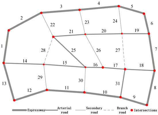
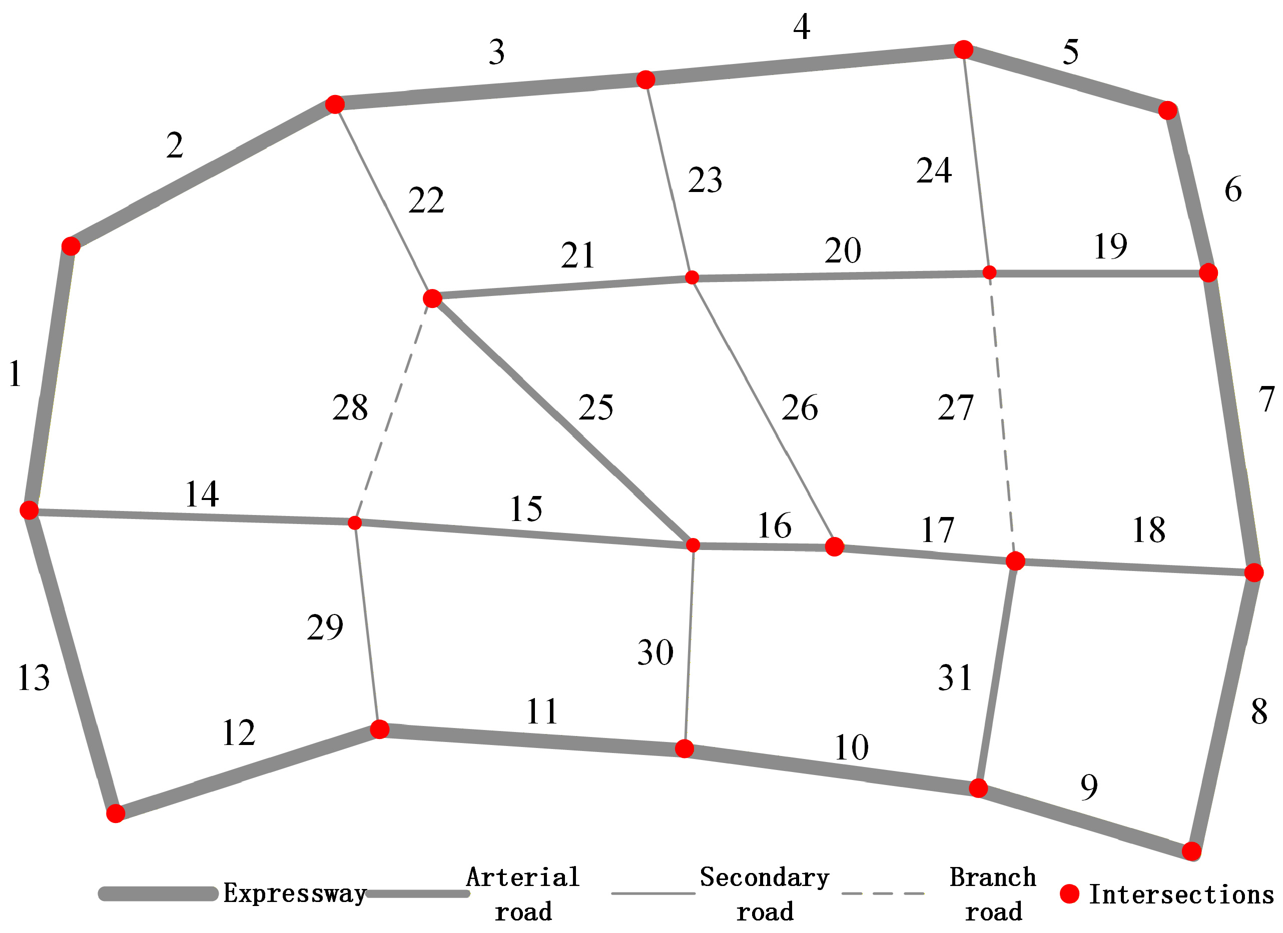
A regional road network in a new district of Nanjing, China, was selected to examine how aggregation rules behave in a heterogeneous network. The network contains 31 road segments covering expressways, arterial roads, secondary roads, and branch roads. Minor roads without regular motor-vehicle observations were not included. The topology and segment identifiers are shown in Figure 1.

Figure 1. Topology and segment identifiers of the selected urban road network.

The four road classes have different mobility and access functions, nominal capacities, and shares of total network length. Their composition is summarized in Table 2. The capacity values are used only for the capacity-km benchmark in Equation (6).

Table 2. Composition and class-level capacity of the selected network.

Class	Segment IDs	Count	Length (km)	Capacity (pcu/h)
Expressway	1–13	13	17.248	1670
Arterial road	14–21, 25, 31	10	11.588	1260
Secondary road	22–24, 26, 29, 30	6	7.703	880
Branch road	27, 28	2	3.076	720
Total	1–31	31	39.615	–

4.2. Data Source and Retained Segment Attributes

The project records identify the source as a one-week traffic survey conducted in September 2024 during weekday evening peak periods from 17:30 to 19:30, excluding weekends. The retained validated records contain road class, segment length, aggregated traffic flow, average speed, and a class-specific capacity value associated with each segment. Traffic flow is expressed in passenger-car units per hour (pcu/h). These values are analyzed only as evening-peak observations from the retained survey week.

The project archive does not preserve the survey technology or sensor source, the exact number of surveyed weekdays or valid observation intervals, whether links were recorded directionally, how observations within 17:30–19:30 were averaged, or how missing values and outliers were handled. It also does not document whether the capacity field is per lane, per direction, or per whole segment, or the source used to assign the four class-specific capacity values. Accordingly, only the validated aggregated segment records are reported; the raw observations are unavailable, and no missing survey detail is reconstructed or imputed. The empirical input should therefore be interpreted as a retained and audited case dataset for demonstrating the aggregation method, rather than as a fully documented traffic-survey dataset from which the original observation protocol can be reconstructed.

Table 3 is the single segment-level input used for all calculations in this manuscript. The final column is the traffic state derived by applying Table 1; it is shown alongside the inputs to make the classification auditable. The product $q_j{L}_j$ is calculated from these retained fields as an observed hourly throughput/exposure rate in pcu·km/h, not as latent demand, user delay, or time-integrated VKT. No result from a previously aggregated network table was carried forward.

Table 3. Audited road-segment inputs and derived baseline traffic states.

ID	Class	Length (m)	Flow (pcu/h)	Speed (km/h)	Capacity (pcu/h)	State
1	Expressway	1489	1480	42.287	1670	Mild congestion
2	Expressway	1517	1467	39.951	1670	Mild congestion
3	Expressway	1263	1373	39.057	1670	Mild congestion
4	Expressway	1367	1435	39.171	1670	Mild congestion
5	Expressway	931	1280	37.462	1670	Mild congestion
6	Expressway	962	1279	38.823	1670	Mild congestion
7	Expressway	1502	750	39.243	1670	Mild congestion
8	Expressway	1650	946	35.804	1670	Mild congestion
9	Expressway	1046	1212	40.425	1670	Mild congestion
10	Expressway	1232	1167	40.674	1670	Mild congestion
11	Expressway	1323	1012	40.192	1670	Mild congestion
12	Expressway	1166	1102	43.735	1670	Mild congestion
13	Expressway	1800	1397	40.872	1670	Mild congestion
14	Arterial road	1388	1152	20.678	1260	Moderate congestion
15	Arterial road	1429	1059	17.671	1260	Moderate congestion
16	Arterial road	625	569	32.875	1260	Mild congestion
17	Arterial road	731	841	40.477	1260	Slightly uncongested
18	Arterial road	975	969	20.864	1260	Moderate congestion
19	Arterial road	939	1189	19.612	1260	Moderate congestion
20	Arterial road	1261	937	35.142	1260	Slightly uncongested
21	Arterial road	1082	1029	18.542	1260	Moderate congestion
22	Secondary road	1220	675	20.992	880	Mild congestion
23	Secondary road	1126	823	14.654	880	Moderate congestion
24	Secondary road	1298	592	22.528	880	Mild congestion
25	Arterial road	1829	995	12.514	1260	Severe congestion
26	Secondary road	1709	774	14.383	880	Moderate congestion
27	Branch road	1718	681	4.181	720	Severe congestion
28	Branch road	1358	713	4.952	720	Severe congestion
29	Secondary road	1194	581	16.439	880	Mild congestion
30	Secondary road	1156	527	18.193	880	Mild congestion
31	Arterial road	1329	1232	19.847	1260	Moderate congestion

The dataset supports segment classification and network aggregation but not intersection-level validation. In particular, no raw trajectories, signal timing, intersection delay, or queue observations are available. The empirical scope is therefore restricted to the segment-to-network problem defined in Section 3.

5. Results

5.1. Data Consistency Audit

Before calculating congestion ratios, all lengths, flows, speeds, capacities, VKT-equivalent exposure values, capacity-km terms, road-priority terms, class weights, and binary congestion indicators were regenerated from the single segment table, Table 3. Segment lengths sum to 39.615 km and VKT-equivalent exposures $q_j{L}_j$ sum to 40,256.850 pcu·km/h. The class-level audit is reported in Table 4.

Table 4. Data consistency audit for network length, VKT-equivalent exposure, and class weights.

Class	Length (km)	Exposure (pcu·km/h)	${\mathit{w}}_{\mathit{g}}$ (%)
Expressway	17.248	21,078.285	52.36
Arterial road	11.588	11,896.047	29.55
Secondary road	7.703	5144.306	12.78
Branch road	3.076	2138.212	5.31
Total	39.615	40,256.850	100.00

As additional denominator checks, total observed segment flow is 31,238 pcu/h, total capacity-km is 52,398.400 pcu·km/h, and the ordinal road-priority denominator is 122.238 priority-km. Recalculation from the audited inputs gives a severe-only $R_{FW}$ of 9.98%, and all revised results use this audited calculation chain.

5.2. Segment States and Congestion Mileage Distribution

The segment states in Table 3 follow the intervals in Table 1. Three boundary classifications warrant explicit confirmation. Segment 20 is an arterial road travelling at 35.142 km/h and is therefore slightly uncongested, not mildly congested. Segments 22 and 29 are secondary roads travelling at 20.992 km/h and 16.439 km/h, respectively, and both are mildly congested.

The resulting mileage distribution is shown in Table 5. Mild congestion covers the largest share of the network (57.41%), followed by moderate congestion (25.18%) and severe congestion (12.38%). No segment is classified as uncongested, while 5.03% of network mileage is slightly uncongested.

Table 5. Overall network mileage distribution by baseline traffic state.

State	Mileage (km)	Share (%)
Uncongested	0.000	0.00
Slightly uncongested	1.992	5.03
Mild congestion	22.741	57.41
Moderate congestion	9.977	25.18
Severe congestion	4.905	12.38
Total	39.615	100.00

Road-class results further show the network’s heterogeneity (Table 6). All expressway mileage is mildly congested. Arterial roads span slightly uncongested through severe states, secondary roads are split between mild and moderate congestion, and both branch-road segments are severely congested. These class differences motivate an aggregation rule that does not treat all road mileage as functionally identical.

Table 6. Mileage distribution of baseline traffic states within each road class.

Class	Slight (%)	Mild (%)	Moderate (%)	Severe (%)
Expressway	0.00	100.00	0.00	0.00
Arterial road	17.19	5.39	61.63	15.78
Secondary road	0.00	63.20	36.80	0.00
Branch road	0.00	0.00	0.00	100.00

5.3. Comparison of Six Benchmark Aggregation Rules

Table 7 reports the six benchmark ratios under the three congestion definitions. For compact table labels, Moderate+ denotes moderate-or-worse congestion and Mild+ denotes mild-or-worse congestion. Under severe-only congestion, the estimates range from 7.01% for road-priority weighting to 12.38% for length-based aggregation. The range shifts to 29.17–37.57% for moderate-or-worse congestion. Under mild-or-worse congestion, all estimates exceed 93%, because all expressway and secondary-road mileage and most arterial mileage satisfy that broader definition.

Table 7. Comparison of six benchmark segment-to-network aggregation rules (%).

Definition	Count	Length	Flow	VKT-eq.	Capacity-km	Priority
Severe-only	9.68	12.38	7.65	9.83	8.62	7.01
Moderate+	35.48	37.57	33.98	35.10	30.56	29.17
Mild+	93.55	94.97	94.31	95.54	95.21	95.11

These differences are not calculation noise. Each rule uses a distinct denominator and therefore represents a different aspect of network operation. The comparison also shows that no aggregation rule can be interpreted independently of the congestion definition: changing from severe-only to moderate-or-worse produces a larger shift than changing among the six rules within either definition.

5.4. Class-Function-Weighted Assessment

Table 8 shows the class-specific length ratios $R_g$ and the resulting $R_{FW}$. With the severe-only definition, expressways and secondary roads contribute zero congested mileage, arterial roads have a class ratio of 15.78%, and branch roads have a class ratio of 100.00%. Combining these ratios with the audited VKT-equivalent exposure shares gives $R_{FW}=9.98\%$.

Table 8. Class-specific congestion ratios and proposed class-function-weighted result (%).

Definition	Expressway	Arterial	Secondary	Branch	${\mathit{R}}_{\mathit{FW}}$
Severe-only	0.00	15.78	0.00	100.00	9.98
Moderate+	0.00	77.42	36.80	100.00	32.89
Mild+	100.00	82.81	100.00	100.00	94.92

The proposed result is 32.89% for moderate-or-worse and 94.92% for mild-or-worse. For all three definitions, $R_{FW}$ falls within the range of the six benchmark estimates, while its two-stage weighting retains an explicit interpretation: $R_g$ measures congested spatial coverage inside a road class and $w_g$ represents that class’s share of VKT-equivalent exposure.

5.5. Threshold Sensitivity and Boundary Segments

The severe-congestion thresholds were perturbed jointly by $\pm 5\%$ and $\pm 10\%$. As shown in Table 9, decreasing the thresholds reduces $R_{FW}$ from 9.98% to 7.63%, whereas increasing them by up to 10% leaves the result unchanged. The decrease occurs because Segment 28 moves out of the severe category when the branch-road severe threshold is reduced below its observed speed of 4.952 km/h.

Table 9. Sensitivity of severe-only $R_{FW}$ to class-specific severe-speed thresholds.

Scenario	Joint Adjustment	${\mathit{R}}_{\mathit{FW}}$ (%)
Scenario 1	$-10\%$	7.63
Scenario 2	$-5\%$	7.63
Baseline	Original thresholds	9.98
Scenario 3	$+5\%$	9.98
Scenario 4	$+10\%$	9.98

The multi-level classification contains additional segments close to state boundaries (Table 10). Segment 20 lies 0.142 km/h above the arterial mild/slightly-uncongested boundary; Segment 28 lies 0.048 km/h below the branch severe boundary; Segment 8 lies 0.804 km/h above the expressway moderate/mild boundary; and Segment 23 lies 0.346 km/h below the secondary mild/moderate boundary. Only Segment 28 changes in the severe-threshold experiment, but the other cases identify where calibration of the full five-state threshold system could alter broader congestion definitions.

Table 10. Road segments nearest to road-class-specific speed boundaries; speed quantities are in km/h.

ID	Class	Speed	Boundary	Gap	State
20	Arterial road	35.142	35	0.142	Slightly uncongested
28	Branch road	4.952	5	0.048	Severe congestion
8	Expressway	35.804	35	0.804	Mild congestion
23	Secondary road	14.654	15	0.346	Moderate congestion

Table 9 supports only the severe-only threshold claim because it perturbs only the severe cutoffs. Table 11 extends the joint test to the cutoff defining each binary outcome. Moderate+ is most responsive because several expressway and secondary-road speeds lie near the mild/moderate boundaries; Mild+ changes only when the wider perturbations cross Segments 16, 20, or 24.

Table 11. Joint sensitivity of $R_{FW}$ to each outcome-defining cutoff (%).

Adjustment	Severe-Only	Moderate+	Mild+
$-10\%$	7.63	28.19	91.17
$-5\%$	7.63	28.19	94.92
Baseline	9.98	32.89	94.92
$+5\%$	9.98	37.90	98.14
$+10\%$	9.98	42.71	98.14

The one-class-at-a-time results in Table 12 isolate the sources of these changes. The severe-only result changes only when the branch-road cutoff reclassifies Segment 28. Positive expressway perturbations drive the Moderate+ increase through Segments 8 and 5, whereas negative secondary-road perturbations drive its decrease through Segments 23 and 26; Segment 29 enters under the $+10\%$ secondary-road test. For Mild+, the responsive boundaries are arterial (Segments 16 and 20) and secondary (Segment 24). Thus, sensitivity depends on boundary concentration and the exposure weight of the affected class, not simply on the total number of segments.

Table 12. One-class-at-a-time cutoff sensitivity of $R_{FW}$ (%). Baseline values are 9.98, 32.89, and 94.92.

Class	Adjustment	Severe-Only	Moderate+	Mild+
Expressway	$-10\%$	9.98	32.89	94.92
Expressway	$-5\%$	9.98	32.89	94.92
Expressway	$+5\%$	9.98	37.90	94.92
Expressway	$+10\%$	9.98	40.73	94.92
Arterial	$-10\%$	9.98	32.89	93.33
Arterial	$-5\%$	9.98	32.89	94.92
Arterial	$+5\%$	9.98	32.89	98.14
Arterial	$+10\%$	9.98	32.89	98.14
Secondary	$-10\%$	9.98	28.19	92.77
Secondary	$-5\%$	9.98	28.19	94.92
Secondary	$+5\%$	9.98	32.89	94.92
Secondary	$+10\%$	9.98	34.87	94.92
Branch	$-10\%$	7.63	32.89	94.92
Branch	$-5\%$	7.63	32.89	94.92
Branch	$+5\%$	9.98	32.89	94.92
Branch	$+10\%$	9.98	32.89	94.92

Table 13 tests the road-priority benchmark under the baseline monotonic hierarchy, a steeper hierarchy, and equal weights. The steeper scheme lowers the severe-only and Moderate+ priority ratios because it increases the relative contribution of expressways, where no segment meets those definitions. Equal weights reduce $R_P$ to the length ratio. The numerical priority benchmark therefore depends on its chosen hierarchy, but the qualitative comparison remains unchanged: weighting assumptions materially affect network diagnosis, and none of these schemes changes $R_{FW}$.

Table 13. Sensitivity of the road-priority benchmark $R_P$ to alternative weights (%).

Scheme	Weights (E/A/S/B)	Severe-Only	Moderate+	Mild+
Baseline monotonic	4/3/2/1	7.01	29.17	95.11
Steeper hierarchy	8/4/2/1	5.12	22.00	96.07
Equal weights	1/1/1/1	12.38	37.57	94.97

6. Discussion

6.1. Why Aggregation Rules Matter

The empirical comparison demonstrates that a network congestion ratio is not a direct property of the segment data alone. It is the product of a congestion definition and an aggregation rule. Under the severe-only definition, the same three severely congested segments yield values from 7.01% to 12.38%. Count weighting is sensitive to how links are divided; length weighting represents spatial coverage; flow and VKT-equivalent exposure weighting represent different forms of observed traffic exposure; and capacity and priority weighting emphasize supplied or intended network function. Reporting a ratio without its numerator and denominator therefore obscures the operational meaning of the diagnosis.

The congestion definition has an even larger effect in this case. Severe-only ratios describe a small set of critical links, whereas mild-or-worse ratios describe broad non-free-flow exposure and exceed 93% under every rule. These are not conflicting findings. They answer different questions about traffic state. The expanded cutoff tests also show that the robustness claim must be outcome-specific: the severe-only result changes only at the branch boundary, whereas Moderate+ and Mild+ respond to different class boundaries. This distinction is consistent with traffic-flow theory, in which local state transitions and network-wide performance are related but not interchangeable [10,26,27].

6.2. Why Function-Weighted Assessment Fits Heterogeneous Networks

The proposed $R_{FW}$ is designed for networks in which road classes have distinct functions. Its class weight gives the expressway, which carries 52.36% of VKT-equivalent exposure, more network influence than branch roads, which carry 5.31%. At the same time, the within-class term remains a length ratio, so one high-flow link does not solely determine the state of an entire road class. The resulting two-stage interpretation is useful when managers need to distinguish the spatial coverage of congestion within a class from the class’s contribution to network movement.

This design is not an accuracy claim. $R_{VKT}$ directly weights every segment by its own $q_j{L}_j$, so a high-flow segment can dominate within its class. $R_{FW}$ first calculates the within-class length ratio $R_g$ and then weights road classes by the exposure share $w_g$. A count ratio remains appropriate when the question concerns the proportion of mapped assets, and $R_{VKT}$ remains appropriate when direct segment-level exposure is the primary outcome. $R_{FW}$ is more interpretable for decisions where road-class function and auditable aggregation are important.

6.3. Relation to Existing Network-Level Approaches

TPI-based analyses provide ordered and interpretable reporting scales that are useful for routine communication and pattern summaries [14,17]. Their reported network state nevertheless depends on the quantity supplied to the scale, whereas the present study makes the preceding segment-to-network aggregation rule the object of analysis. MFD-based methods capture aggregate network regimes and production–accumulation relationships when richer dynamic observations and suitable network partitioning are available [10,11,20]. Spatial clustering, zone delineation, and congestion-propagation methods add information about where congestion concentrates and how it spreads across time and space [12,13,15,16,21].

The present method occupies a narrower data regime. It gains auditability and reproducibility because every classification, numerator, denominator, class weight, and perturbation can be reconstructed from one aggregated segment table. That gain is accompanied by clear losses: the retained data cannot describe temporal network regimes, queue accumulation, spillback, or propagation paths. The method should therefore complement rather than replace TPI, MFD, clustering, or propagation analysis when the observations required by those approaches are available.

6.4. Implications for Data-Limited Traffic Management

The method can be implemented with attributes commonly retained in traffic inventories and peak-period surveys. Managers can first inspect class-specific states, then report several benchmark ratios to reveal sensitivity to the chosen operational perspective, and finally use $R_{FW}$ when functional road hierarchy is central to the decision. Boundary-segment reporting is equally important because it directs attention to locations where a small calibration change can alter a discrete label.

For the case network, the results suggest different diagnostic priorities at different scales. Severe congestion is concentrated on two branch segments and one arterial segment, while mild-or-worse conditions extend across nearly the entire network. A severe-only ratio can therefore support critical-link screening, whereas the broader definitions can support monitoring of network-wide operating pressure. Such transparent diagnosis is a prerequisite for targeted mobility and congestion management, which may also help limit delay-related energy use and emissions [28,29,30,31].

6.5. Limitations

This study has five main limitations. First, it evaluates a single 31-segment network, so the numerical ordering of aggregation rules should not be generalized to other networks without additional cases. In a network with hundreds of segments, the influence of one boundary segment is expected to be diluted when road-class exposure shares are balanced and that segment represents a small share of its class mileage. Concentrated boundary segments, long segments, or affected segments in high-weight classes may still shift the aggregate. This scaling behavior should be tested empirically across multiple networks rather than assumed from the present case.

Second, the observations cover weekday evening peak periods during one survey week and cannot establish temporal stability. The hourly exposure shares $w_g$ may vary by time of day, day type, event conditions, or season. The reported weights must therefore be interpreted as evening-peak weights for the retained survey week, not as stable all-day network weights. Third, only validated aggregated segment records are available; the survey technology, interval-level observations, and raw trajectories are absent. Fourth, there is no intersection-level delay or queue dataset, so the analysis cannot validate intersection congestion or propagation mechanisms. Fifth, all discrete results depend on road-class speed thresholds, as demonstrated by Segment 28 and the other boundary segments.

Future work should evaluate the same aggregation protocol across multiple networks and time periods, calibrate thresholds with local historical distributions, and compare the data-limited ratios with trajectory-, detector-, and intersection-based measures when those observations are available. These extensions would test external validity without changing the present study’s bounded claim.

7. Conclusions

Methodologically, this study shows that a network congestion diagnosis is jointly determined by the congestion definition and the aggregation rule. Holding all 31 segment classifications fixed, the benchmark comparison and outcome-specific perturbations demonstrate that changes in either analytical choice can materially alter the reported network ratio.

The proposed $R_{FW}$ provides an auditable two-stage interpretation suited to road-function-based decisions: it measures congested-length coverage within each class and applies observed hourly exposure shares only between classes. This makes the method more interpretable for decisions where road-class function and auditable aggregation are important; the present study does not rank methods by accuracy.

For the 31-segment Nanjing case, $R_{FW}$ is 9.98%, 32.89%, and 94.92% under the severe-only, moderate-or-worse, and mild-or-worse definitions, respectively; the six severe-only benchmarks range from 7.01% to 12.38%. These numerical findings are specific to the retained evening-peak survey week and should not be generalized without additional networks and periods. Future multi-network studies should test scaling, temporal variation in $w_g$, and correspondence with dynamic detector-, trajectory-, queue-, or propagation-based measures.

References

- National Academies of Sciences, Engineering and Medicine. Highway Capacity Manual 7th Edition: A Guide for Multimodal Mobility Analysis; The National Academies Press: Washington, DC, USA, 2022. [Google Scholar] [CrossRef] [Scilit] [PubMed]
- Federal Highway Administration. Documentation and Definitions—Urban Congestion Reports. Available online: https://ops.fhwa.dot.gov/perf_measurement/ucr/documentation.htm (accessed on 8 May 2026).
- Gore, N.; Arkatkar, S.; Joshi, G.; Antoniou, C. Developing modified congestion index and congestion-based level of service. Transp. Policy 2023, 131, 97–119. [Google Scholar] [CrossRef] [Scilit]
- Parry, I.W.H.; Walls, M.; Harrington, W. Automobile externalities and policies. J. Econ. Lit. 2007, 45, 373–399. [Google Scholar] [CrossRef] [Scilit]
- Yang, S.; Ji, Y.; Zhang, D.; Fu, J. Equilibrium between road traffic congestion and low-carbon economy: A case study from Beijing, China. Sustainability 2019, 11, 219. [Google Scholar] [CrossRef] [Scilit]
- Rahman, M.M.; Najaf, P.; Fields, M.G.; Thill, J.-C. Traffic congestion and its urban scale factors: Empirical evidence from American urban areas. Int. J. Sustain. Transp. 2022, 16, 406–421. [Google Scholar] [CrossRef] [Scilit]
- He, F.; Yan, X.; Liu, Y.; Ma, L. A traffic congestion assessment method for urban road networks based on speed performance index. Procedia Eng. 2016, 137, 425–433. [Google Scholar] [CrossRef] [Scilit]
- Wang, W.-X.; Guo, R.-J.; Yu, J. Research on road traffic congestion index based on comprehensive parameters: Taking Dalian city as an example. Adv. Mech. Eng. 2018, 10, 1687814018781482. [Google Scholar] [CrossRef] [Scilit]
- Jiang, J.; Chen, Q.; Xue, J.; Wang, H.; Chen, Z. A novel method about the representation and discrimination of traffic state. Sensors 2020, 20, 5039. [Google Scholar] [CrossRef] [Scilit] [PubMed]
- Geroliminis, N.; Daganzo, C.F. Existence of urban-scale macroscopic fundamental diagrams: Some experimental findings. Transp. Res. Part B Methodol. 2008, 42, 759–770. [Google Scholar] [CrossRef] [Scilit]
- Daganzo, C.F.; Geroliminis, N. An analytical approximation for the macroscopic fundamental diagram of urban traffic. Transp. Res. Part B Methodol. 2008, 42, 771–781. [Google Scholar] [CrossRef] [Scilit]
- Saeedmanesh, M.; Geroliminis, N. Dynamic clustering and propagation of congestion in heterogeneously congested urban traffic networks. Transp. Res. Part B Methodol. 2017, 105, 193–211. [Google Scholar] [CrossRef] [Scilit]
- Saberi, M.; Hamedmoghadam, H.; Ashfaq, M.; Hosseini, S.A.; Gu, Z.; Shafiei, S.; Nair, D.J.; Dixit, V.; Gardner, L.; Waller, S.T.; et al. A simple contagion process describes spreading of traffic jams in urban networks. Nat. Commun. 2020, 11, 1616. [Google Scholar] [CrossRef] [Scilit] [PubMed]
- Zang, J.; Jiao, P.; Liu, S.; Zhang, X.; Song, G.; Yu, L. Identifying traffic congestion patterns of urban road network based on traffic performance index. Sustainability 2023, 15, 948. [Google Scholar] [CrossRef] [Scilit]
- Loo, B.P.Y.; Huang, Z. Delineating traffic congestion zones in cities: An effective approach based on GIS. J. Transp. Geogr. 2021, 94, 103108. [Google Scholar] [CrossRef] [Scilit]
- Shi, Y.; Wang, D.; Tang, J.; Deng, M.; Liu, H.; Liu, B. Detecting spatiotemporal extents of traffic congestion: A density-based moving object clustering approach. Int. J. Geogr. Inf. Sci. 2021, 35, 1449–1473. [Google Scholar] [CrossRef] [Scilit]
- DB11/T 785–2011; Urban Road Traffic Performance Index. Standards Press of China: Beijing, China, 2011.
- GA/T 115–2020; Evaluation Methods for Road Traffic Congestion Levels. Ministry of Public Security: Beijing, China, 2020.
- Daganzo, C.F. Urban gridlock: Macroscopic modeling and mitigation approaches. Transp. Res. Part B Methodol. 2007, 41, 49–62. [Google Scholar] [CrossRef] [Scilit]
- Ji, Y.; Geroliminis, N. On the spatial partitioning of urban transportation networks. Transp. Res. Part B Methodol. 2012, 46, 1639–1656. [Google Scholar] [CrossRef] [Scilit]
- Hamedmoghadam, H.; Zheng, N.; Li, D.; Vu, H.L. Percolation-based dynamic perimeter control for mitigating congestion propagation in urban road networks. Transp. Res. Part C Emerg. Technol. 2022, 145, 103922. [Google Scholar] [CrossRef] [Scilit]
- Han, X.; Shen, G.; Yang, X.; Kong, X. Congestion recognition for hybrid urban road systems via digraph convolutional network. Transp. Res. Part C Emerg. Technol. 2020, 121, 102877. [Google Scholar] [CrossRef] [Scilit]
- Hu, Q.; Liu, Y.; Guo, T. Spatiotemporal distribution pattern recognition model for urban traffic congestion situation monitoring. J. Transp. Syst. Eng. Inf. Technol. 2012, 12, 41–45. (In Chinese) [Google Scholar]
- Bai, H.; Wang, J.; Jiang, Y. Evaluation of highway network traffic operation state based on point, line and area. China J. Highw. Transp. 2018, 31, 197–204. (In Chinese) [Google Scholar]
- Federal Highway Administration. Traffic Congestion and Reliability: Trends and Advanced Strategies for Congestion Mitigation; FHWA-HOP-05-064; U.S. Department of Transportation: Washington, DC, USA, 2005.
- Lighthill, M.J.; Whitham, G.B. On kinematic waves II. A theory of traffic flow on long crowded roads. Proc. R. Soc. A Math. Phys. Eng. Sci. 1955, 229, 317–345. [Google Scholar] [CrossRef] [Scilit]
- Richards, P.I. Shock waves on the highway. Oper. Res. 1956, 4, 42–51. [Google Scholar] [CrossRef] [Scilit]
- Banister, D. The sustainable mobility paradigm. Transp. Policy 2008, 15, 73–80. [Google Scholar] [CrossRef] [Scilit]
- Barth, M.; Boriboonsomsin, K. Real-world carbon dioxide impacts of traffic congestion. Transp. Res. Rec. J. Transp. Res. Board 2008, 2058, 163–171. [Google Scholar] [CrossRef] [Scilit]
- Grote, M.; Williams, I.; Preston, J.; Kemp, S. Including congestion effects in urban road traffic CO2 emissions modelling: Do local government authorities have the right options? Transp. Res. Part D Transp. Environ. 2016, 43, 95–106. [Google Scholar] [CrossRef] [Scilit]
- Bharadwaj, S.; Ballare, S.; Rohit; Chandel, M.K. Impact of congestion on greenhouse gas emissions for road transport in Mumbai metropolitan region. Transp. Res. Procedia 2017, 25, 3538–3551. [Google Scholar] [CrossRef] [Scilit]
Disclaimer/Publisher’s Note: The statements, opinions and data contained in all publications are solely those of the individual author(s) and contributor(s) and not of MDPI and/or the editor(s). MDPI and/or the editor(s) disclaim responsibility for any injury to people or property resulting from any ideas, methods, instructions or products referred to in the content. |
© 2026 by the authors. Licensee MDPI, Basel, Switzerland. This article is an open access article distributed under the terms and conditions of the Creative Commons Attribution (CC BY) license.