Article

Evaluation of Anchor Axial Force Prediction Methods for Pile-Anchor Retaining Structures Based on Field Monitoring and FEM

1
College of Civil Engineering, Hainan University, Haikou 570228, China
2
Hainan Engineering Consulting and Design Group Co., Ltd., Haikou 570206, China
3
Hainan Design Institute Co., Ltd., Haikou 571924, China
*
Author to whom correspondence should be addressed.
Appl. Sci. 2026, 16(17), 8800; https://doi.org/10.3390/app16178800
Submission received: 10 May 2026 / Revised: 24 August 2026 / Accepted: 27 August 2026 / Published: 4 September 2026
(This article belongs to the Section Civil Engineering)

Abstract

Pile-anchor retaining systems represent a fundamental support technology for urban deep excavations, where accurate quantification of anchor axial force is essential to achieving both structural safety and economical design. Here, we systematically assessed the predictive performance of several established design approaches—namely the static equilibrium method, the equivalent beam method, the earth pressure envelope method, an empirical chart-based method, and the CPD method—against in-situ monitoring data acquired from a deep excavation project. Under the site-specific conditions, the chart-based method delivered the closest agreement with the measured anchor forces. We further implemented a finite element model to perform a parametric sensitivity analysis, elucidating the influence of anchor embedment depth, excavation depth, and groundwater table position on anchor axial force. The results revealed that increasing anchor embedment depth produced only a marginal variation in anchor force, indicating weak sensitivity. In contrast, deepening the excavation produced a pronounced escalation in anchor force and significantly modulated pile bending moments. Elevating the depth to the groundwater table (i.e., lowering the water level) caused the anchor force to decline monotonically, with the rate of decrease progressively attenuating at greater depths, thereby demonstrating a moderate dependency on groundwater conditions.

1. Introduction

Pile-anchor systems constitute the predominant retention strategy for medium to deep excavations. In these configurations, retaining piles provide flexural rigidity while prestressed anchor cables absorb lateral earth pressures, collectively delivering high load-bearing capacity, stringent deformation control, and construction efficiency—attributes that have driven their widespread deployment across diverse excavation projects. Early international contributions laid the mechanistic groundwork: Rowe analyzed the structural behavior of anchored sheet-pile walls, developed internal force models, and delineated the distribution of the anchor tension and pile bending moment [1]; Sowers et al. consolidated design philosophies for anchored structures and formulated the load-transfer mechanism along the anchor bond length [2]; O’Rourke and Jones, through sustained field monitoring, resolved the influence of excavation sequence and tendon tensioning on the force and deformation response of the retaining system, providing a valuable observational benchmark [3].
With respect to practical calculation methods, numerous procedures have been advanced internationally, progressively refining the theoretical design apparatus. Peck introduced the earth pressure envelope method, enabling rapid estimation of lateral earth loads [4]; Hagerty and Nofal devised a chart-based procedure that simplifies parameter selection [5]; LaCroix and Atmatzidis synthesized design approaches for anchored retaining walls and issued selection guidance tailored to distinct engineering scenarios [6]; Das et al. systematically catalogued various computational methods for pile-anchor systems in their textbook, clarifying the domain of applicability for each [7]. These approaches are complemented by normative documents—most notably the FHWA anchored system guidelines [8], Eurocode 7 [9], and China’s Technical Specification for Retaining and Protection of Building Foundation Excavations [10]—which collectively codify the design of pile-anchor retaining structures. Beyond these codified methods, alternative analytical frameworks have also been developed internationally. For instance, Bouassida and Porbaha employed the kinematic approach of yield design theory combined with three-dimensional scaled model tests to investigate the ultimate bearing capacity of soft clays reinforced by a group of deep mixing columns, deriving closed-form upper and lower bound solutions for the bearing capacity factor [11].
Utilizing China’s complex geological settings, domestic researchers have generated a substantial body of original work. Li quantified the conditions under which separate versus combined earth-and-water pressure calculations should be adopted, thereby supporting the subsequent analysis of earth pressures [12]. Zheng’s group, through model tests and field measurements, revealed the progressive collapse mechanisms triggered by local anchor failure and proposed corresponding early-warning indicators and reinforcement strategies [13]. Cheng et al. experimentally simulated the sequential collapse of a pile-anchor-supported excavation, establishing the patterns of moment redistribution within the retaining piles and the abrupt shifts in anchor axial force [14]. For specialized conditions, Hao et al. conducted in-situ experiments on composite micro-pile–anchor–strut systems and optimized their design parameters in miscellaneous fill strata [15]. Wang et al. examined the dynamic response and seismic damage evolution of pile-anchor retaining structures under earthquake loading, proposing seismic optimization measures [16], and Ding et al. further investigated the seismic resilience of such systems [17]. For structures subjected to uplift loading, Kumar et al. conducted field tests on single and group granular anchor pile systems, demonstrating the influence of length-to-diameter ratio and pile spacing on pullout capacity, which provides a useful reference for understanding the load-transfer mechanisms in anchored retaining systems [18].
Substantial headway has also been made in refining computational methods. Yang, Zhang, and co-workers proposed an incremental approach that explicitly incorporates the progressive excavation sequence, closely reproducing actual construction stages [19]. Zhou et al. advanced an improved incremental-iterative method that integrates nonlinear soil parameters to enhance predictive accuracy and streamline the computational workflow, and validated its rationality through MATLAB 2018B implementation and PLAXIS finite-element simulations [20]. Complementing these analytical and numerical approaches, Rashid et al. employed a discontinuity layout optimization (DLO) method coupled with a homogenization technique to develop preliminary design charts for deep mixing reinforced soils, systematically examining the influence of improvement area ratio, cohesion ratio, and reinforcement depth on bearing capacity [21]. Furthermore, practice-oriented research has calibrated pile-anchor design and construction procedures for typical regional projects in Qingdao and other areas [22]. Despite these advances, the applicability of the available methods varies considerably, and the mechanical behavior and deformation control under atypical loading or geometric conditions still demand deeper investigation.
Against this backdrop, the present study selects a representative suite of calculation methods, subjects them to an initial screening through a theoretical benchmark comparison, and then rigorously evaluates their performance against field monitoring data acquired from a deep excavation project in Hainan. A finite-element–based parametric sensitivity analysis is subsequently performed. The primary objective is to assess the practical applicability of each method under the specific geological and construction conditions of this project, and to provide preliminary guidance for anchor axial force prediction in comparable sandy soil settings.

2. Anchor Axial Force Prediction Methods

2.1. Static Equilibrium Method

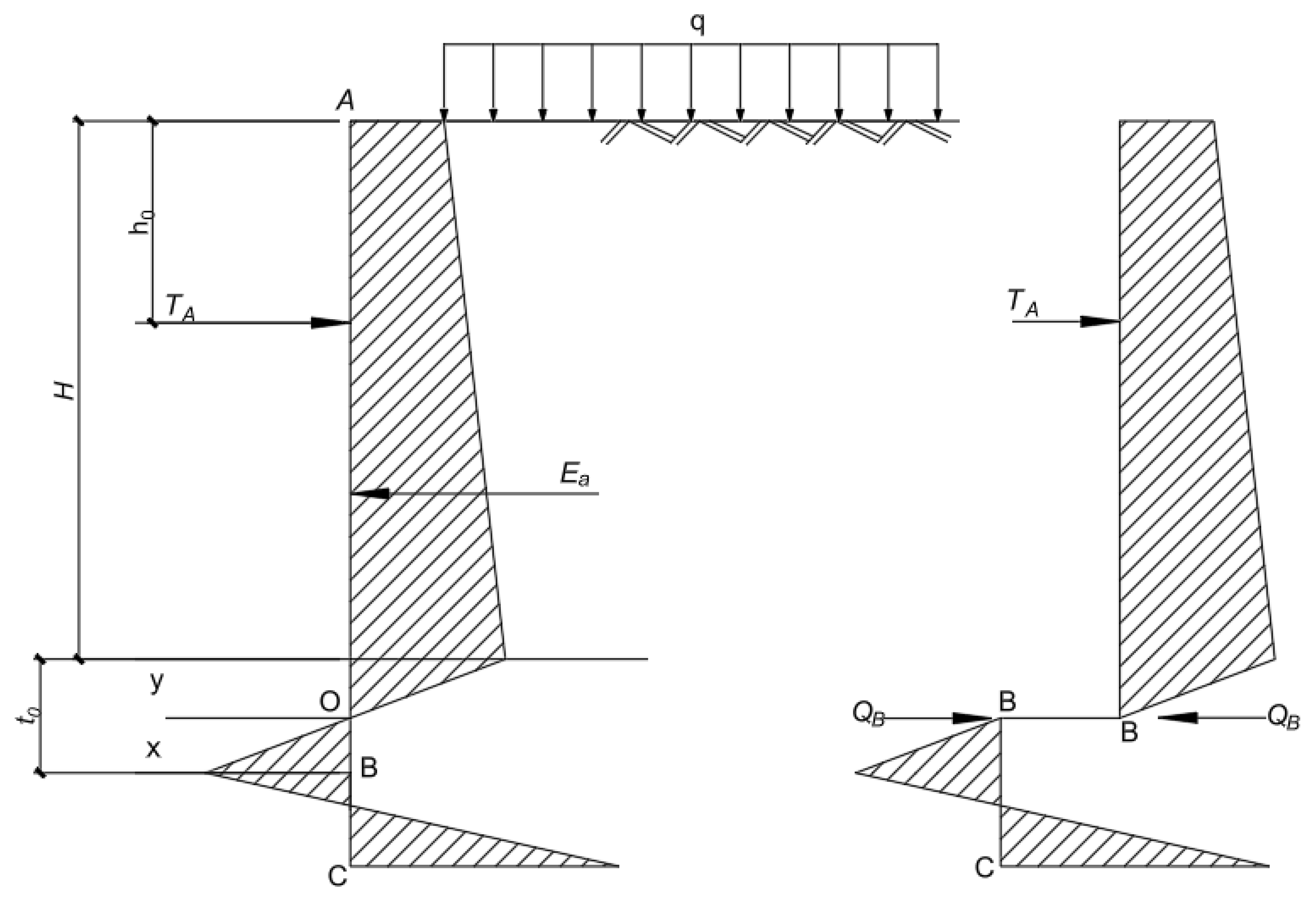
The static equilibrium method is founded in limit equilibrium theory, establishing force equilibrium of the retaining structure to resolve the distribution of internal forces and earth pressures. This approach is codified in China’s Technical Specification for Retaining and Protection of Building Foundation Excavations (JGJ 120-2012) and remains one of the most widely deployed design procedures in current practice. Internationally, the method shares conceptual foundations with the limit state design framework embedded in Eurocode, insofar as both derive from soil limit states; they diverge, however, in the adopted safety factors and the architecture of the partial factor system. Computationally, the pile is idealized as a statically determinate, simply supported beam with a single overhang: the pile tip is treated as a simple support, the single anchor level as a vertical restraint, and the entire retaining pile thus reduces to a simply supported cantilever model. The solution procedure is straightforward—the anchor horizontal force and the required embedment depth are taken as the primary unknowns, and two equilibrium equations, one for horizontal force balance and one for global moment equilibrium, are formulated. Solving this system directly delivers the unknowns, after which the internal force distribution along the pile is recovered using elementary structural mechanics. In this formulation, the earth resistance acting on the excavation side is conventionally evaluated by the classical method, with the underlying principle schematically depicted in Figure 1.

2.2. Equivalent Beam Method

The equivalent beam method idealizes the retaining pile as a beam on an elastic foundation and captures soil restraint by introducing a subgrade reaction coefficient. Conceptually, this method constitutes an engineering adaptation of the classical beam-on-elastic-foundation theory. Internationally, analogous elastic foundation analyses—most notably those founded on the Winkler model—are routinely employed in the United States, Japan, and elsewhere. Relative to the Chinese equivalent beam method, these international variants typically place greater emphasis on the rational selection and nonlinear calibration of soil stiffness parameters. The entire retaining pile is modeled as a statically indeterminate cantilever beam that incorporates a lateral support. For a single-anchor wall with an elastically restrained base, the position of zero net earth pressure lies in close proximity to the point of zero bending moment; accordingly, the pile can be notionally severed at the point of zero net earth pressure and analyzed as two interconnected statically determinate beams in Figure 2.

2.3. Force Polygon Graphical Method

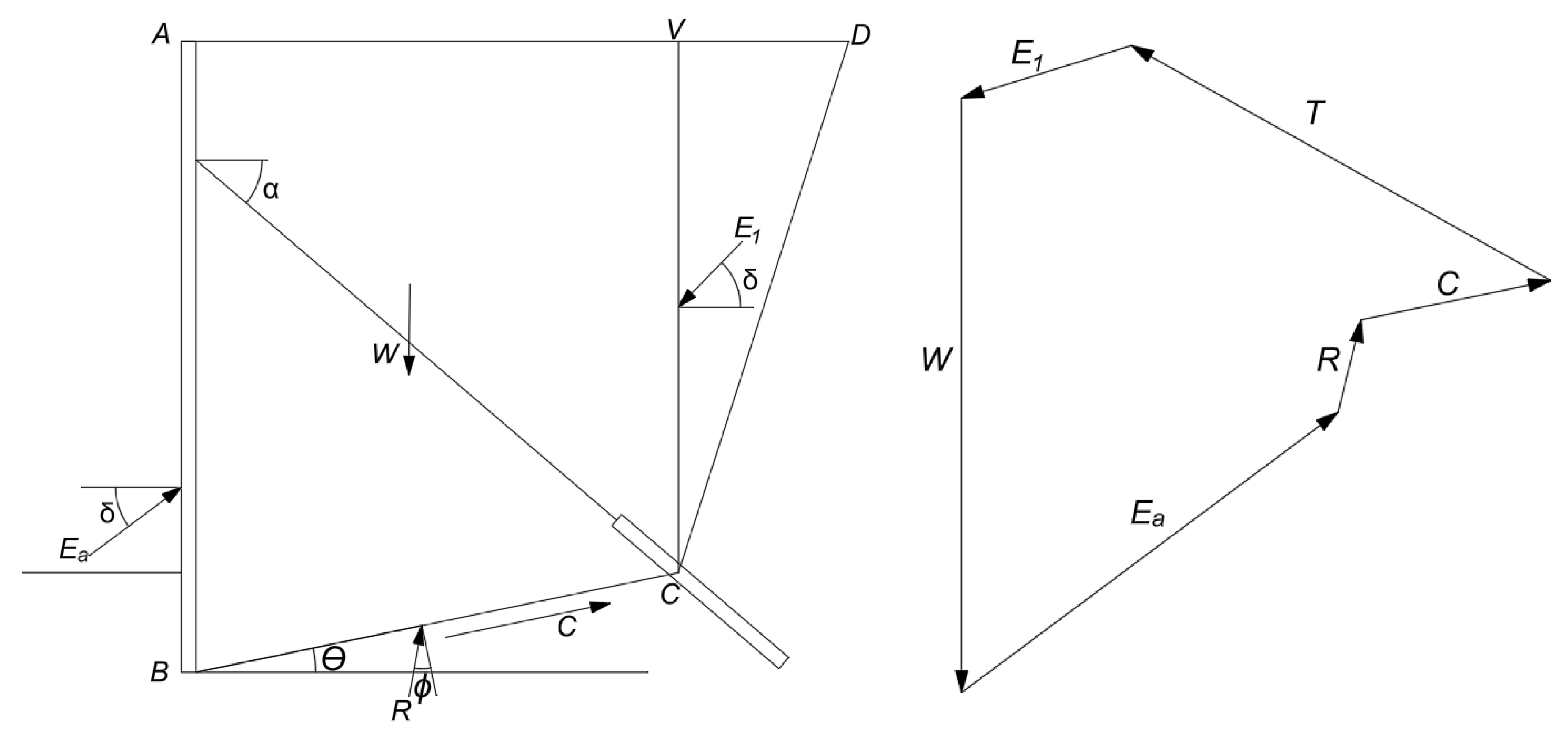
A planar wedge comprising the pile, anchor, and surrounding soil is isolated from the ground as a free body, and the tensile force carried by the anchor is determined from the equilibrium of this wedge using a force polygon construction. The principle is illustrated in Figure 3: a straight line BC is drawn connecting the centroid C of the anchor bond zone to an assumed virtual pivot B at the base of the retaining pile; this line BC is taken to represent the deep-seated sliding surface. A vertical line CV is then extended upward from point C. The resulting wedge ABCV is subjected to its self-weight W and to additional force components—schematically denoted F, C, etc.—and, when the wedge attains a state of limit equilibrium, the maximum anchor tension T is obtained directly from the closure of the force polygon. This construction explicitly incorporates anchor design parameters such as the incidence angle, free length, and total anchor length. In engineering practice, the graphical method serves primarily as a stability-verification tool; because the present study focuses on calculation methods intended for theoretical design, this approach is not further elaborated here.

2.4. Earth Pressure Envelope Method

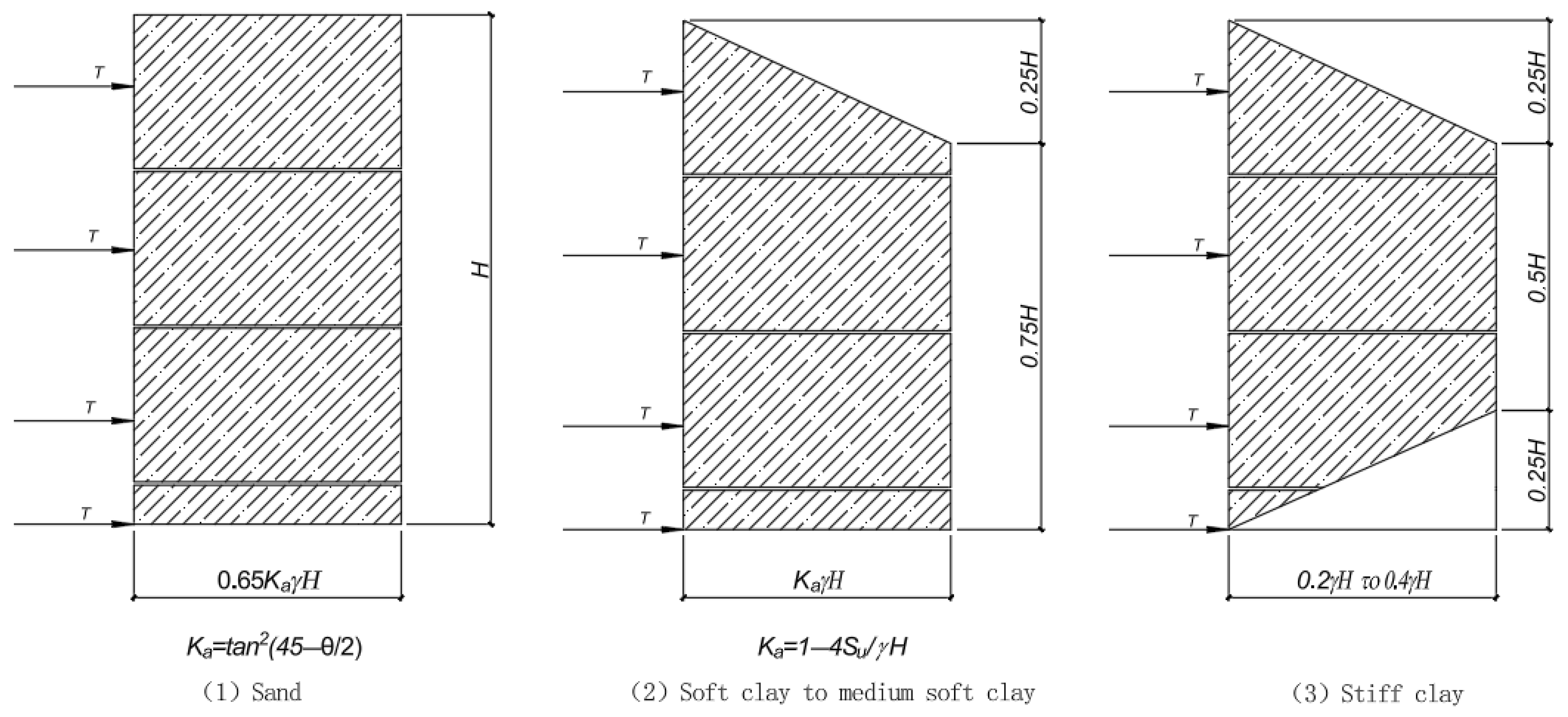
The earth pressure envelope method was originally introduced by Terzaghi and Peck (1967, 1969) [4,23], who back-calculated apparent pressure distributions from field measurements of strut loads in internally braced excavations. It constitutes a semi-empirical design procedure that permits anchor loads and wall bending moments to be estimated through comparatively straightforward manual computation. The published envelopes represent pressure distributions inferred from field-measured strut loads in Table 1.
For sand, Terzaghi and Peck’s charts yield a total lateral earth load of 0.65 Kaγ H2, which can be expressed as an apparent earth pressure coefficient multiplied by γ H2. For walls retained by a single anchor level or by two or more anchor levels, the recommended apparent earth pressure envelope adopts a trapezoidal configuration; in sand, a rectangular distribution is prescribed, with the total lateral load taken as 1.3 times the Rankine active earth pressure—a choice that represents a deliberate, empirically founded conservatism. As illustrated in Figure 4, for an excavation supported by multiple rows of anchors, the total lateral load employed to determine the maximum apparent earth pressure is taken as the horizontal component of the load derived from limit equilibrium analysis.
The method is computationally straightforward and consequently enjoys widespread adoption in engineering practice. Owing to its reliance on empirical idealizations, however, the fidelity of the predictions can deteriorate under complex geological conditions or in non-routine construction scenarios.

2.5. Chart-Based Method

Hagerty and Nofal (1992) [5] introduced a rapid estimation procedure for anchor forces in sands, derived from a systematic dimensionless parameter analysis anchored in a substantial database of empirical observations and statistical correlations. The method delivers earth pressure distributions and structural internal forces through a series of pre-computed charts, substantially streamlining the design workflow. Its computational simplicity renders it particularly valuable during preliminary design stages. Conceptually, the approach shares a conceptual origin with the excavation deformation envelopes pioneered by Peck, which extract generalized deformation patterns from extensive field measurements and have exerted considerable influence on international practice. By normalizing key parameters—anchor elevation, excavation depth, groundwater table position, and surcharge—the chart-based method establishes relationships between a generalized anchor force and a suite of correction factors, thereby avoiding the need for iterative computation.
Input parameters: excavation depth Z d , anchor elevation Z a , depth to groundwater table Z w , internal friction angle φ , average unit weight γ a , and surcharge pressure Q .
γ a = γ m Z d Z w + γ s u b Z w Z d
where γ m = unit weight above the water table, and γ s u b = effective unit weight below the water table.
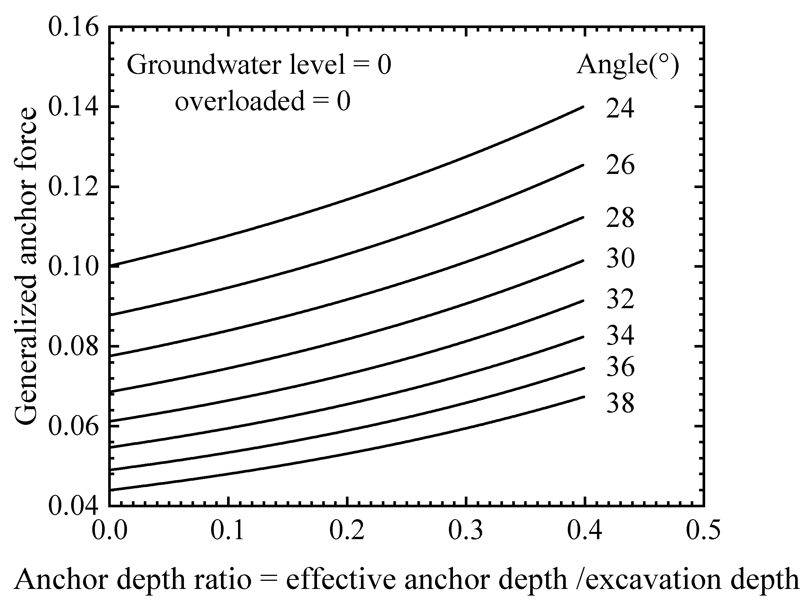
The generalized anchor force G A p (valid for Q   =   0 ,   Z w   =   0 ) is read from charts using Z a / Z d and φ (Figure 5).
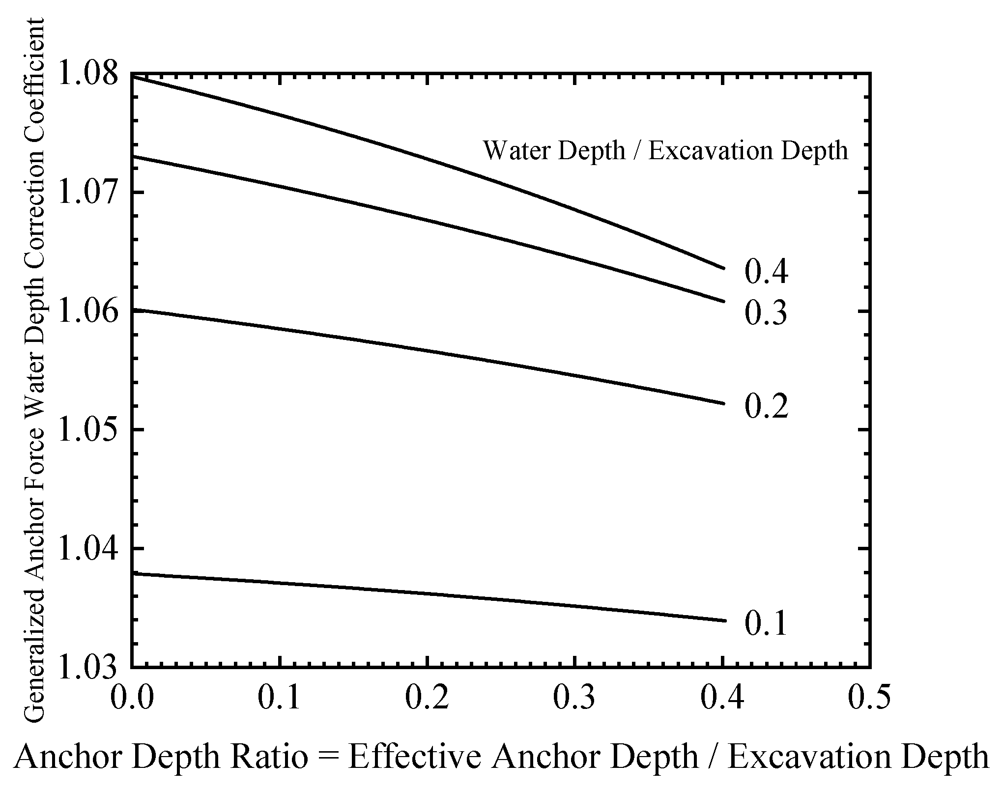
A water-level correction factor C A Z w is obtained from Figure 6, entered with Z a / Z d and Z w / Z d .
A surcharge correction factor C A p Q is interpolated from Table 2 based on φ and Z a / Z d .
The corrected generalized anchor force is computed as:
corrected G A P   =   G A P   1 + C A p Q   Q C A Z w
and the actual anchor force follows directly:
A p   =   corrected G A p   γ a   Z d 2
While the chart-based method offers considerable computational efficiency and reasonable accuracy for sandy strata, its extension to other soil types or to complex, non-idealized conditions necessitates further verification and calibration.

2.6. Computed Pressure Diagram (CPD) Method

The Computed Pressure Diagram method refines conventional earth pressure theory by modifying the idealized pressure distribution to better capture the variation in lateral earth pressures under diverse construction conditions, thereby yielding predictions that more closely reflect observed field behavior. This strategy aligns with an evolving international research trend that leverages field monitoring data to iteratively calibrate earth pressure models, progressively enhancing predictive fidelity through empirical feedback. In constructing the analytical framework, the method exploits effective stress principles in sand: the inherently nonlinear distributions of active and passive earth pressure are idealized as equivalent rectangular blocks. Two correction factors are introduced—an earth pressure modification factor C, which reconciles discrepancies between the theoretical and actual pressure distributions, and a passive-to-active pressure ratio R, which simplifies the evaluation of passive resistance. These idealizations transform the complex integration of pressure diagrams into rudimentary algebraic manipulation of rectangular areas. Applying horizontal force equilibrium and moment equilibrium then yields a closed-form relationship linking the anchor horizontal force to the sheet-pile embedment depth.
The average net active earth pressure σ a behind the wall needs to be corrected using the empirical coefficient C, and the formula is
σ a = C K a γ a v L
where γ a v = average effective unit weight (weighted for layered profiles), L = excavation depth, and C = empirical correction coefficient. The values are adjusted according to the compaction of the sand, with detailed figures shown in Table 3.
The net passive pressure in front of the wall is related to active pressure through the pressure ratio R :
σ p = R σ a
with R ranging from 0.3–0.5 (loose), 0.55–0.65 (medium), or 0.60–0.75 (dense).
Horizontal force equilibrium requires that the anchor force F (per unit length) balances the net resultant:
F = σ a L R D
Moment equilibrium about the anchor point yields the embedment depth D :
D 2 + 2 D L 1 l 1 L L 2 R 1 2 l 1 L = 0
where l 1 = anchor height above the pit bottom. The method’s simplicity comes at the cost of approximating complex pressure distributions, and the empirical coefficients introduce subjectivity that can affect accuracy.

2.7. Theoretical Design Calculation: Comparative Benchmarking

To rigorously evaluate the theoretical accuracy and mutual divergence of the candidate methods on a common footing, this chapter constructs a standardized computational model deliberately stripped of site-specific complexities, thereby focusing the analysis squarely on the theoretical core of each approach.

2.7.1. Computational Model

Model parameters are adapted from the worked example presented by Das and Sivakugan in Principles of Foundation Engineering, 9th edition [7], Section 18.12. The critical parameters are as follows: excavation depth set to 5.0 m; groundwater table located at 2.0 m depth, with the simplifying assumption that the water level inside and outside the excavation is identical; anchor design depth 1.0 m below the top of the excavation; surcharge at the ground surface taken as 0 kPa; soil moist unit weight 15.9 kN/m3; saturated unit weight 19.33 kN/m3; and internal friction angle 32°. The average unit weight was computed via the standard formula, converting the moist and effective unit weights into an equivalent uniform value to streamline and preserve the accuracy of lateral earth pressure calculations; for the present example, the average unit weight was determined as 13.6 kN/m3.
We implemented each theoretical method as an independent computational function on a programming platform. All methods received an identical set of model parameters and directly output the design anchor axial force.

2.7.2. Computational Results and Comparative Analysis

The theoretical results produced by the various methods are summarized in Table 4. The data reveal pronounced discrepancies, with the predicted anchor forces spanning a broad range.
A preliminary inspection reveals that the equivalent beam method, the CPD method, and the chart-based method yield relatively tightly clustered values, indicating a degree of internal consistency in their theoretical treatment of sand loading. The static equilibrium method returns a result appreciably higher than these three; its simplifying assumption that neglects pile–soil interaction constitutes the principal source of this overestimation. The earth pressure envelope method produces a value far exceeding all others, vividly illustrating its built-in empiricism-driven conservatism—the design load is deliberately inflated to envelop a wide spectrum of uncertainties.
This theoretical benchmark comparison serves to preliminarily isolate a subset of methods—the chart-based method, the equivalent beam method, and the CPD method—that generate reasonably plausible results. The true fidelity of these candidates under real field conditions, however, must be substantiated through subsequent validation against an instrumented excavation case.

2.8. Field Case Comparative Analysis

2.8.1. Computational Model of the Pile-Anchor Retaining Structure

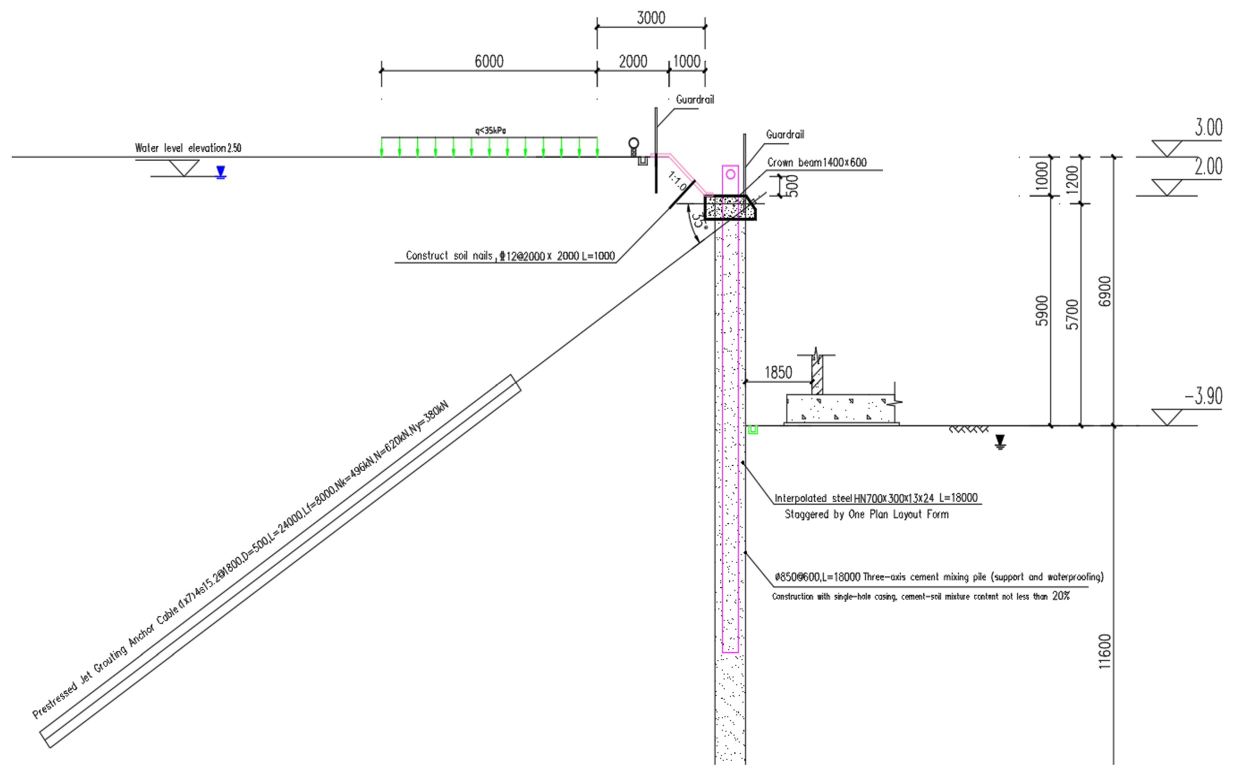
The north cross-section of a deep excavation executed for a construction project in Hainan was selected for detailed analysis. On this side, the earth retention employed a rigid soil-cement mixed wall reinforced with embedded steel sections (SMW pile wall), which, in conjunction with a single level of prestressed anchor cables, constituted an anchored retaining system. The computational model was configured to faithfully incorporate the in-situ conditions. The excavation depth was 6.9 m, and the design groundwater table was set at an elevation of 2.5 m. A 6-m-wide strip surcharge, not exceeding 35 kPa, was present at a distance of 3 m from the excavation edge. To streamline the analysis, the 1-m-high berm above the pile top (graded at 1:1) and any additional surcharge acting on the berm were consolidated into an equivalent uniform surcharge of 30 kPa. The embedded steel member comprised a hot-rolled H-beam of grade Q235 with a nominal section HN700×300×13×24. The anchor system consisted of a single row of four 15.2 mm seven-wire strands (1 × 7) installed at an incidence angle of 35°; the total anchor length was 24 m with a free length of 8 m, arranged at a horizontal spacing of 1.8 m and a vertical spacing of 1.2 m. The recommended design parameters for the ground layers are summarized in Table 5, and the cross-sectional profile of the retaining system is depicted in Figure 7.
Stratigraphically, sand layers dominate the excavation profile. Guided by the site investigation and laboratory test results, the physical and mechanical parameters of the sand strata were adopted for computation. These parameters were input into the custom-programmed calculation routines; the anchor axial forces yielded by the equivalent beam method, the computed pressure diagram (CPD) method, and the chart-based method are compiled in Table 6.
The results in Table 6 reveal pronounced divergence among the three theoretical predictions: the equivalent beam method yields 266.4 kN, the chart-based method 200.2 kN, and the CPD method 239.6 kN. The chart-based method gives the lowest estimate, whereas the equivalent beam method gives the highest—a difference of 66.2 kN, corresponding to a relative spread of approximately 33.1%. For a single engineering object, such widely scattered estimates, stemming purely from the choice of design theory, confront practitioners with a non-trivial dilemma.
From a mechanistic standpoint, the equivalent beam method produces an upper-bound prediction largely because it idealizes the pile tip as a fixed support and severs the pile at the point of zero net earth pressure to reduce it to a statically determinate beam; this simplification overestimates the degree of structural restraint and consequently drives the anchor force toward a conservative extreme. The CPD method collapses the intricate pressure distribution into a rectangular envelope and introduces empirical coefficients C and R for adjustment; its result falls between those of the equivalent beam and chart-based methods, yet the selection of empirical coefficients retains a measure of subjectivity, and variations in their prescribed values can perturb the outcome. The chart-based method, through systematic parameter normalization and multi-variate correction, explicitly accommodates the coupled influence of anchor position, excavation depth, groundwater level, surcharge, and the internal friction angle—affording, in principle, a more complete parametric framework.
Critically, theoretical divergence does not inherently validate or invalidate any individual method; the decisive question is which prediction most closely reproduces the observed field response. Resolving this question mandates rigorous validation against in-situ monitoring data to establish the accuracy and practical applicability of each theoretical approach.

2.8.2. On-Site Engineering Monitoring Results

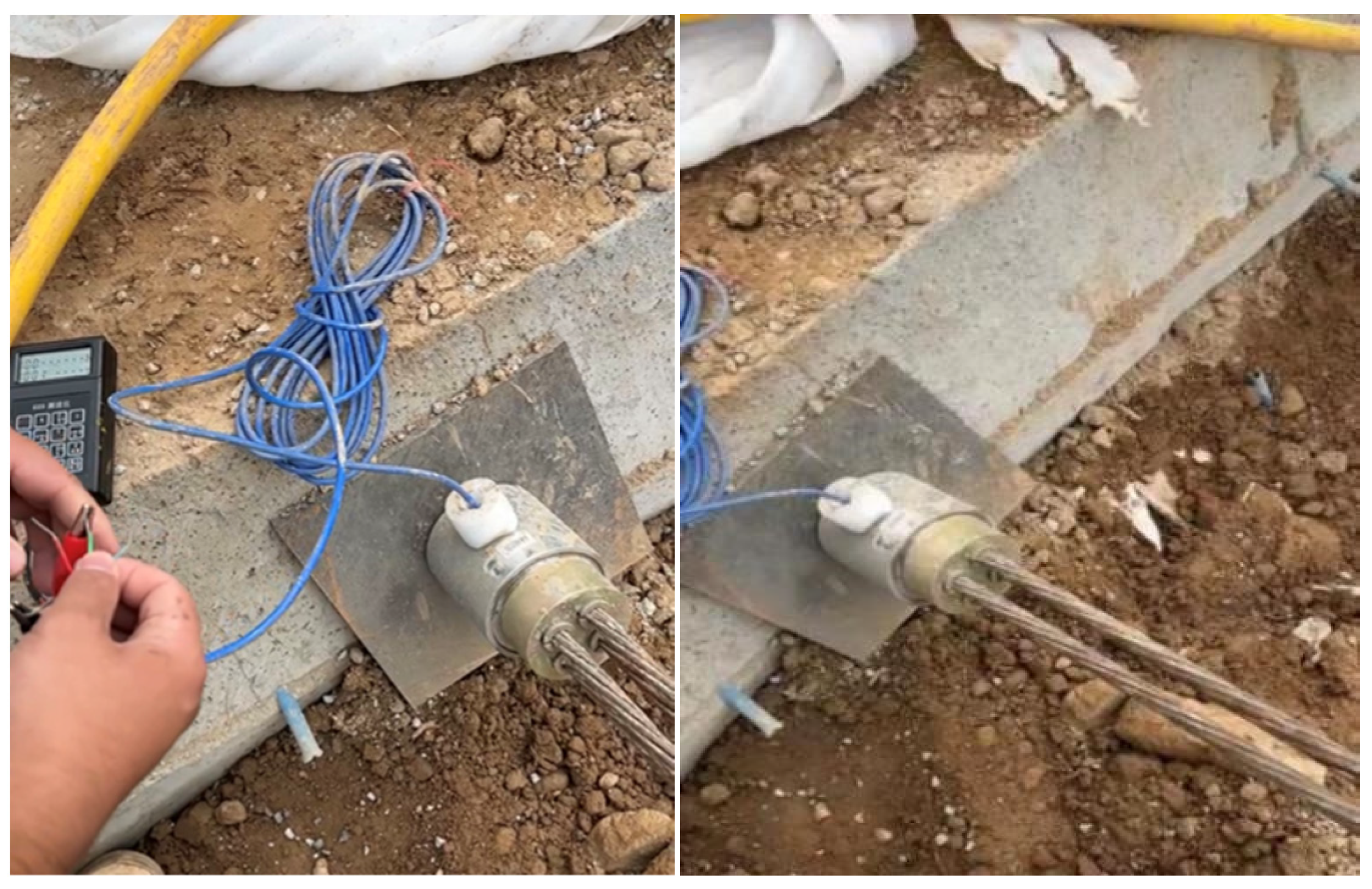
In the present project, vibrating-wire anchor load cells were installed on representative anchors and monitored continuously from post-tensioning lock-off through excavation backfilling in Figure 8.
The readout cables were routed to a monitoring station at the excavation crest, where they were systematically labeled, secured, and shielded to prevent construction-related damage that could compromise data integrity. Readings were acquired with a high-precision frequency readout unit offering an accuracy of 0.5% full scale and a resolution of 0.2% full scale, satisfying the rigors of engineering monitoring. Initial frequencies were logged immediately before and after prestressing, and the resulting axial forces were subsequently calibrated against the tensioning jack calibration certificate to eliminate systematic bias. Throughout the measurement campaign, the acquisition timing and temperature were stringently controlled to minimize environmentally induced perturbations. Each load cell was interposed between the anchor head and the bearing plate; the resonant frequency of its internal tensioned steel wire shifts in response to the applied tensile force and is captured by a frequency readout device (model 609A), from which the anchor axial force is derived. Prior to and following lock-off, baseline readings were recorded, and all instruments were safeguarded for the duration of construction. These load cells constitute the most direct empirical evidence for validating the design theories of pile-anchor retaining systems.
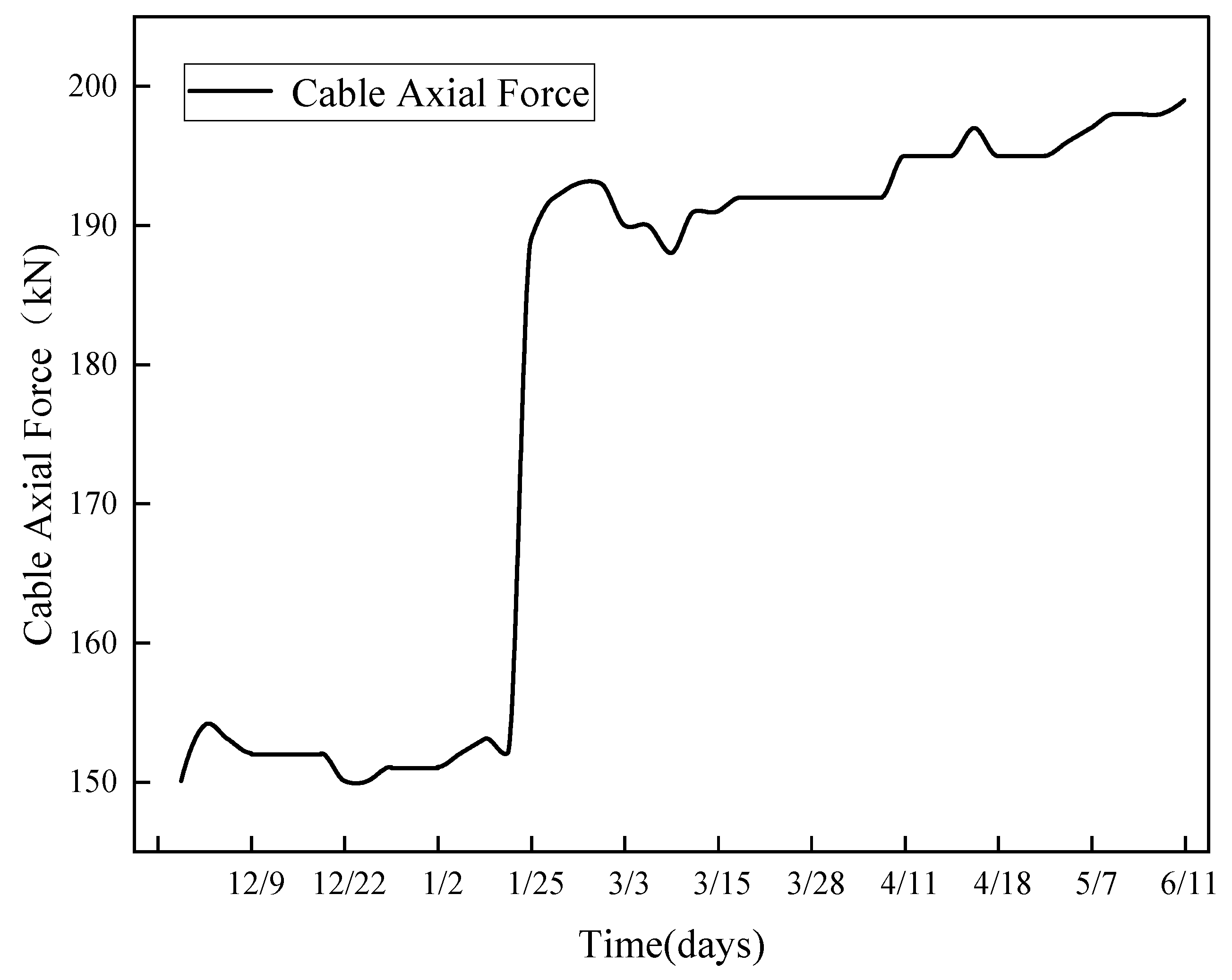
Figure 9 delineates the characteristic evolution of anchor axial force throughout the construction sequence. Upon tensioning to the design lock-off load, a modest prestress loss manifests within a short period, a response attributable to material relaxation and soil creep and recognized as routine. As the excavation proceeds downward in successive lifts, the axial force exhibits a pronounced stepwise escalation. Each discrete increment marks the removal of soil beneath the anchor level, the concomitant release of lateral earth pressure, and its subsequent transfer to the anchor; the measured curve thus graphically captures the intrinsic “excavation-while-supporting” load-carrying mechanism of the retaining system. Once the excavation reaches the design formation level and the base slab is cast, excavation-induced deformations stabilize, the anchor axial force ceases to rise appreciably, and it subsequently settles into a narrow, stationary fluctuation band.
After rigorous data screening and reduction, the long-term average monitoring value of 199 kN, acquired under steady-state excavation conditions, was adopted as the field-derived benchmark for the anchor service load. This value, having been purged of transient construction-induced perturbations and measurement noise, faithfully represents the force sustained by the retaining structure at the serviceability limit state and provides an objective, defensible basis for theoretical validation.

2.8.3. Comparison of Calculated Values and Field-Measured Data

The theoretical predictions of the three selected methods are benchmarked against the anchor axial force of 199 kN derived from field monitoring; the quantitative assessment is summarized in Table 7, which articulates the accuracy and practical suitability of each approach.
The results presented in Table 7 reveal the following:
The chart-based method yields a value of 200.2 kN, deviating from the measured benchmark by only +0.6%—the highest fidelity achieved among the three candidates. This outcome indicates the favourable performance of the chart-based method in the sandy strata encountered in Hainan. Central to its performance is a systematic normalization of anchor elevation, excavation depth, groundwater table position, and surcharge, augmented by empirical corrections; the combined deployment of the three core parameters—the generalized anchor force, the surcharge correction factor, and the water-level correction factor—effectively reduces model uncertainty and enables a more faithful reproduction of the complex pile–anchor–soil interaction mechanisms that prevail in sand.
The equivalent beam method returns a predicted force of 266.4 kN, corresponding to an overestimation of +33.9% and reflecting a distinctly conservative bias. The source of this overprediction lies largely in its foundational assumption that the point of contraflexure coincides with the point of zero bending moment—an idealization that loses precision in the heterogeneous, nonlinear ground conditions of the field. Moreover, the method does not adequately capture the nonlinear deformation response of the soil, driving the anchor force estimate toward an upper bound.
The CPD method gives an intermediate value of 239.6 kN, with a +20.4% deviation. By collapsing the intrinsically nonlinear earth pressure distribution into a rectangular envelope, the method achieves computational simplicity at the expense of introducing appreciable model error. Additionally, the empirical coefficients and the passive-to-active pressure ratio embedded in the CPD framework carry a measure of subjectivity; the choice of values for sands of differing relative densities can noticeably perturb the final result.
A comprehensive comparison establishes the following accuracy ranking: chart-based method (+0.6%) > CPD method (+20.4%) > equivalent beam method (+33.9%). The high precision attained by the chart-based method clearly attests to its applicability and reliability in the sandy strata of Hainan and provides a robust theoretical basis for the design of pile-anchor composite retaining systems in this region.

3. Finite Element Numerical Simulation

To further investigate the mechanical response of the pile-anchor retaining structure under varying design parameters and to establish a reliable computational platform for subsequent parametric sensitivity analysis, a two-dimensional plane-strain finite element model was developed using the geotechnical finite element software PLAXIS 2D 2024. This chapter presents a comprehensive description of the model development, parameter selection, construction stage simulation procedures, and validation against field monitoring data.

3.1. Model Development

3.1.1. Geometry and Boundary Conditions

A two-dimensional plane-strain finite element model of the pile-anchor composite retaining system was constructed. The model domain was set to 100 m in length and 50 m in height, with the origin located at the intersection of the slope crest and the wall top (x-axis positive to the right, y-axis positive downward). These dimensions were determined in accordance with Saint-Venant’s principle to ensure that boundary effects on the computational results in the zone of interest are negligibly small.
Boundary conditions were applied as follows: Bottom boundary: Fully fixed in both horizontal and vertical directions (ux = uy = 0). Left and right lateral boundaries: Roller supports with horizontal displacement restrained and vertical displacement permitted (ux = 0, uy ≠ 0), simulating the far-field conditions of a semi-infinite soil mass.
Ground surface: Free boundary, allowing both vertical and horizontal displacements.
These boundary conditions are consistent with standard practices in deep excavation modelling. Preliminary trial calculations confirmed that, with the adopted model dimensions, the boundaries have negligible influence on the stress and displacement fields near the retaining structures.

3.1.2. Element Type and Mesh Generation

Fifteen-node triangular elements were selected for the global mesh. This element type provides significantly higher-fidelity stress fields for problems involving complex geometries and stress concentrations (e.g., stress redistribution due to excavation, pile-soil interaction, and anchor bond zones), albeit at a commensurately greater computational expense. The analysis employs a displacement-based formulation with 15-node interpolation shape functions and 12th-order Gaussian integration.
Mesh sensitivity analysis was conducted to balance computational accuracy and efficiency. Three mesh densities were tested in Table 8.
The results indicate that the medium and fine meshes differ by only 0.7%, which is well within acceptable engineering tolerances. Considering both accuracy and computational efficiency, the medium-dense mesh scheme (14,200 nodes and 6800 fifteen-node triangular elements) was adopted for formal calculations.
Local mesh refinement was applied in the following regions: near the excavation face (horizontal range: x = −5 m to +5 m, depth range: ground surface to 10 m below the excavation bottom); surrounding the retaining wall (SMW pile wall) and within 2 m on both sides; around the anchor bond zones; near the slope crest and toe.
Element sizes transition gradually from 0.3 m in the refined zones to 5.0 m in the far-field regions.

3.1.3. Constitutive Model

The Mohr–Coulomb elastic-perfectly plastic model was adopted as the constitutive model for the soil. The yield function is expressed as:
τ = c + σ n t a n ϕ
where τ is the shear strength, c is the cohesion, σn is the normal stress, and ϕ is the internal friction angle. An associated flow rule was employed, with the plastic potential function consistent with the yield function.
The Mohr–Coulomb model was selected for the following reasons: (1) its parameters have clear physical meanings and can be directly obtained from conventional laboratory tests (direct shear tests, triaxial tests, etc.), facilitating engineering application; (2) extensive studies have demonstrated that, for internal force analysis of retaining structures, the Mohr–Coulomb model yields predictions that are in close agreement with field monitoring data, satisfying engineering accuracy requirements; (3) compared with more sophisticated constitutive models (e.g., hardening soil models or small-strain stiffness models), the Mohr–Coulomb model offers significantly higher computational efficiency, which is particularly advantageous for iterative parametric sensitivity analyses.
Limitation acknowledgement: The Mohr–Coulomb model, as an elastic-perfectly plastic model, does not capture the stress-dependent stiffness or the small-strain stiffness decay characteristics of soils. In deep excavation problems dominated by unloading, this model tends to overestimate surface settlements behind the wall, while its predictions of wall lateral displacements remain generally acceptable. Since the primary focus of this study is the internal force analysis of the retaining structure—particularly anchor axial forces—rather than detailed predictions of ground surface settlements, the Mohr–Coulomb model provides a reasonable balance between accuracy and computational efficiency for the present purposes. It is noteworthy that alternative modeling approaches have been successfully applied to related geotechnical problems. Jellali et al. developed a homogenization method within the yield design theory framework to estimate the bearing capacity of soft soils reinforced by a group of columns, deriving macroscopic strength criteria and their upper/lower bound estimates. This approach offers a complementary theoretical perspective for analyzing soil–structure interaction problems in deep excavation contexts [24].

3.1.4. Groundwater Modelling

The groundwater table at the site is located at a depth of 2.5 m (i.e., Z w = 2.5 m). A steady-state pore pressure distribution was adopted. Negative pore pressures (suction) were assigned above the water table, while hydrostatic pore pressures were applied below the water table according to:
u = γ w ( y y w )
where y is the depth at the calculation point, y w is the groundwater table depth, and γ w = 10 kN / m 3 is the unit weight of water.
Simplification: For the short-term excavation simulation, the groundwater flow was assumed to have reached a steady state; transient pore pressure dissipation and hydro-mechanical coupling effects were not considered. The effective stress principle was applied for soil below the water table, with the effective unit weight γ = γ s a t γ w used in mechanical calculations. Dewatering inside the excavation (to a final depth of 7.4 m) was simulated by adjusting the pore pressure boundary conditions in the excavation zone at the corresponding construction stage.

3.1.5. Initial Stress Generation

The initial in-situ stress field was generated using the K 0 procedure (gravity loading method). After model construction, gravitational loading was applied in conjunction with the lateral earth pressure coefficient K 0 to generate the initial horizontal stress field. The K 0 values were determined as follows:
Sandy soil layers: Jaky’s formula K 0 = 1 s i n ϕ , where ϕ is the effective internal friction angle.
Cohesive layer (muddy silty clay): K 0 = 0.6 , based on the overconsolidation ratio (OCR ≈ 1.0–1.2, normally consolidated) and local engineering experience.
The generated initial stress field must satisfy static equilibrium under self-weight. After equilibrium, the maximum unbalanced displacement was approximately 3.2 × 10 5 m, and the maximum unbalanced force ratio was less than 1.0 × 10 3 , meeting the computational requirements.
All nodal displacements were then reset to zero to establish the initial condition for subsequent excavation simulations, ensuring that all subsequent displacement outputs represent incremental displacements caused by construction activities.

3.1.6. Convergence Criteria

The numerical analysis employed a Newton–Raphson iterative solution scheme in Table 9. Convergence was assessed using a combination of displacement and energy criteria.
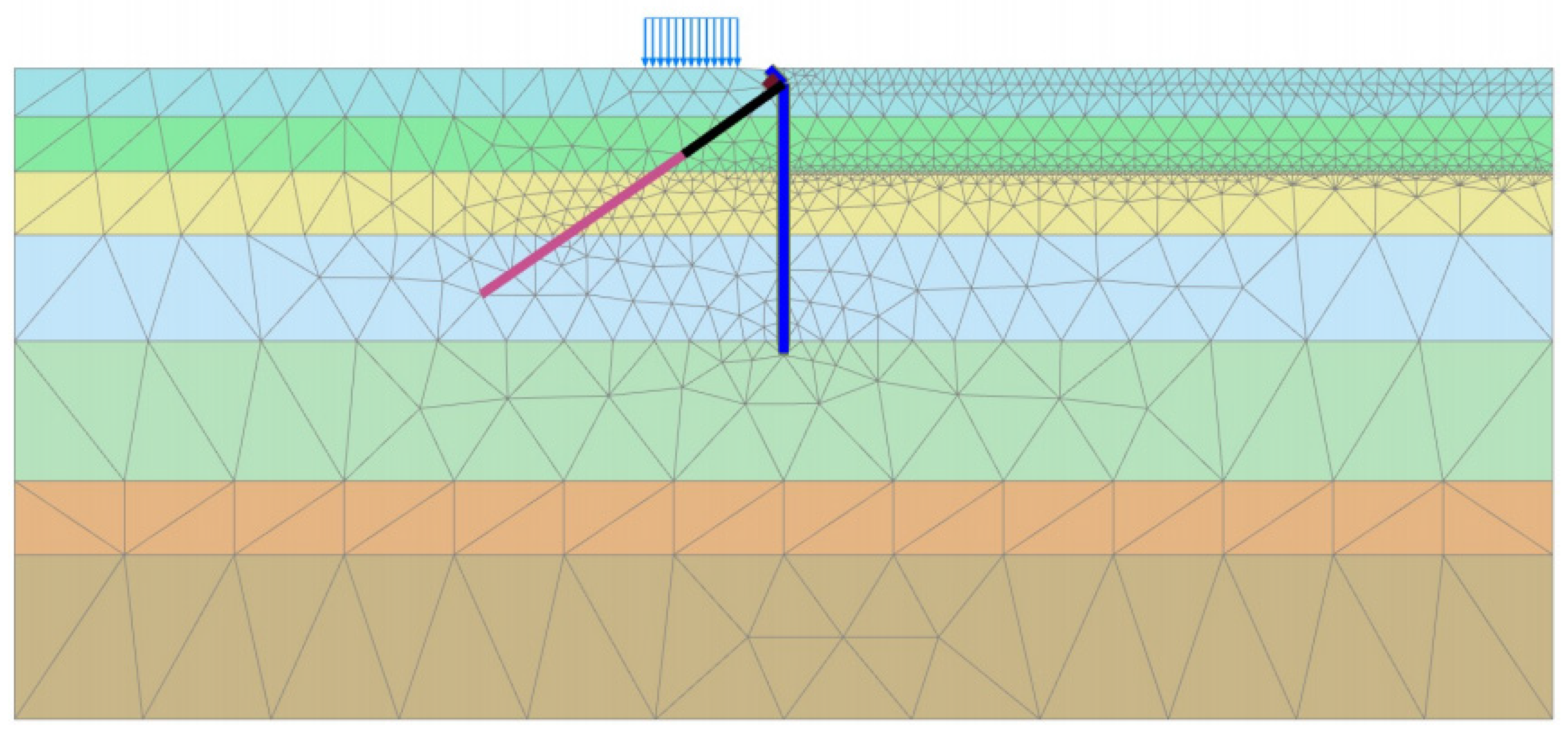
The maximum number of iterations per increment was set to 40. When convergence was not achieved within 30 iterations, adaptive sub-stepping was automatically activated, subdividing the current calculation step into smaller sub-steps, each subject to the same convergence criteria. Convergence histories were monitored in real time to ensure that each step satisfied the criteria before proceeding to the next construction stage. The connection diagram of foundation pit support model is shown in Figure 10.

3.2. Model Parameters

All input parameters were sourced directly from the design documents and the site investigation report; their faithful translation into computational equivalents is the key factor of simulation realism.

3.2.1. Soil Layer Parameters

Soil material parameters were adopted straight from the recommended values tabulated in Table 5. The elastic modulus E was derived from the compression modulus E s using the empirical relationship E = 2 ~ 5 E s , assigning the upper end of the range to sandy soils and the lower end to cohesive soils. Poisson’s ratio ν was selected according to soil-type-specific empiricism (e.g., 0.25–0.35 for sands, 0.30–0.40 for clays) in Table 10. All parameters were then tabulated and input into the material database.

3.2.2. Retaining Structure Parameters

1. The SMW pile wall consists of H-beams inserted into triaxial cement-soil columns. To simplify the numerical representation and adopt a conservative approach, only the contribution of the H-steel sections to the wall stiffness was explicitly accounted for; the cement-soil was assumed to provide primarily the hydraulic cut-off function and a nominal degree of soil improvement, without contributing to structural stiffness.
Equivalence principle: The discretely arranged H-beams were homogenized into a continuous, uniform elastic plate (plate element). The equivalence requires that the equivalent plate, when subjected to identical axial forces and bending moments, produces exactly the same deformation response as the original composite wall.
Calculation procedure:
Step 1: Steel section properties
Grade Q235 hot-rolled H-beams (model HN700×300×13×24) were used, with the following sectional properties as summarized in Table 11.
Step 2: Number of beams per unit width
The design center-to-center spacing of the H-beams is s = 0.9 m. Thus, the number of beams per meter width is:
n = 1 s = 1 0.9 1.111   beams / m
Step 3: Equivalent axial stiffness ( E A ) e q per meter width
( E A ) e q = n × E s t e e l × A s = 1.111 × ( 2.06 × 10 8 ) × ( 231.5 × 10 4 ) 5.29 × 10 6   kN / m
Step 4: Equivalent flexural stiffness ( E I ) e q per meter width
( E I ) e q = n × E s t e e l × I s = 1.111 × ( 2.06 × 10 8 ) × ( 197000 × 10 8 ) 4.50 × 10 5   kN · m 2 / m
Step 5: Equivalent thickness d
The equivalent thickness is a derived quantity, used primarily for visualization and self-weight calculation:
d = 12 × ( E I ) e q ( E A ) e q = 12 × 4.50 × 10 5 5.29 × 10 6 1.01   m
2. The anchor system was modelled using a combination of node-to-node anchor elements and embedded pile elements to represent the tensile behaviour of the free length and the bond-slip behaviour of the grouted zone, respectively.
① Free length (node-to-node anchor element)
The anchor consists of four strands of Φ15.2 mm seven-wire steel strands (nominal cross-sectional area A s t r a n d = 140 mm2 each). The total cross-sectional area is:
A f = 4 × 140 = 560   mm 2 = 5.60 × 10 4   m 2
The elastic modulus of the steel strand is E f = 1.95 × 10 8 kPa.
The axial stiffness of the free length is:
( E A ) f r e e = E f × A f = 1.95 × 10 8 × 5.60 × 10 4 1.092 × 10 5   kN
This value is directly assigned as the axial stiffness of the node-to-node anchor element. The anchor spacing is 1.8 m horizontally; in the plane-strain model, this was converted to a per-meter-width basis: 1.092 × 10 5 / 1.8 6.07 × 10 4 kN/m/m.
The anchor inclination angle is 20°, and the prestressing force is applied at Stage 3 with a lock-off load of 320 kN (80% of the design tensile load of 480 kN).
② Bond length (embedded pile element)
The bond length is a composite of the grout body and surrounding soil, simulated using embedded pile elements to capture the soil–grout interface interaction. The bearing capacity is governed by the ultimate skin friction at the interface.
Ultimate skin friction calculation:
Based on the site investigation report, the bond length passes through the following layers:
The thickness-weighted average ultimate bond strength is:
q s k , a v g = 4.0 × 120 + 6.0 × 30 4.0 + 6.0 = 84   kPa
The grout body diameter is d b o n d = 0.15 m (from design documents). The ultimate skin friction per unit length is:
f m a x = q s k , a v g × ( π × d b o n d ) = 84 × ( 3.1416 × 0.15 ) 39.6   kN / m
The detailed parameters of the anchor bond length are presented in Table 12.
This value is assigned as the ultimate interface shear strength of the embedded pile element. Within the elastic range, the axial stiffness of the grout body itself is set to a high value ( E b o n d = 1.0 × 10 7 kPa) to focus the analysis on the soil–grout interface load transfer.
The choice of embedded pile elements for modelling the bond length is justified by the following considerations. First, this element type effectively captures the axial skin friction transfer along the grout–soil interface, which is the primary load-transfer mechanism governing anchor axial capacity—the key output of interest in this study. Second, although embedded pile elements may introduce some degree of artificial local pinning in two-dimensional plane-strain analyses, this effect has limited influence on the present results because: (i) the focus is on the global axial force response of the anchor rather than local stress distributions around the bond zone; (ii) the embedded pile formulation in PLAXIS 2D 2024 has been extensively validated in geotechnical practice for anchor and pile simulations; and (iii) alternative approaches—such as geogrid elements or solid elements with modified properties—either cannot adequately represent the bond-slip mechanism (geogrid) or would substantially increase computational cost without commensurate improvement in axial force predictions (solid elements). Based on these considerations, the embedded pile element represents a reasonable compromise between computational efficiency and acceptable accuracy for the present purposes.
3. Interface elements were established between the SMW pile wall (plate elements) and the surrounding soil. Interface strength properties were defined using a reduction factor R i n t e r :
Interface cohesion: c i n t e r f a c e = R i n t e r × c s o i l
Interface friction angle: ϕ i n t e r f a c e = R i n t e r × ϕ s o i l
4. Based on local engineering experience, R i n t e r = 0.7 was adopted to reasonably simulate the potential relative slip between the wall and the soil. The normal and shear stiffnesses of the interface were set to ten times the stiffness of the adjacent soil to minimize spurious deformation while maintaining numerical stability. The parameters of all structural components are summarized in Table 13.

3.3. Simulation of Construction Stages

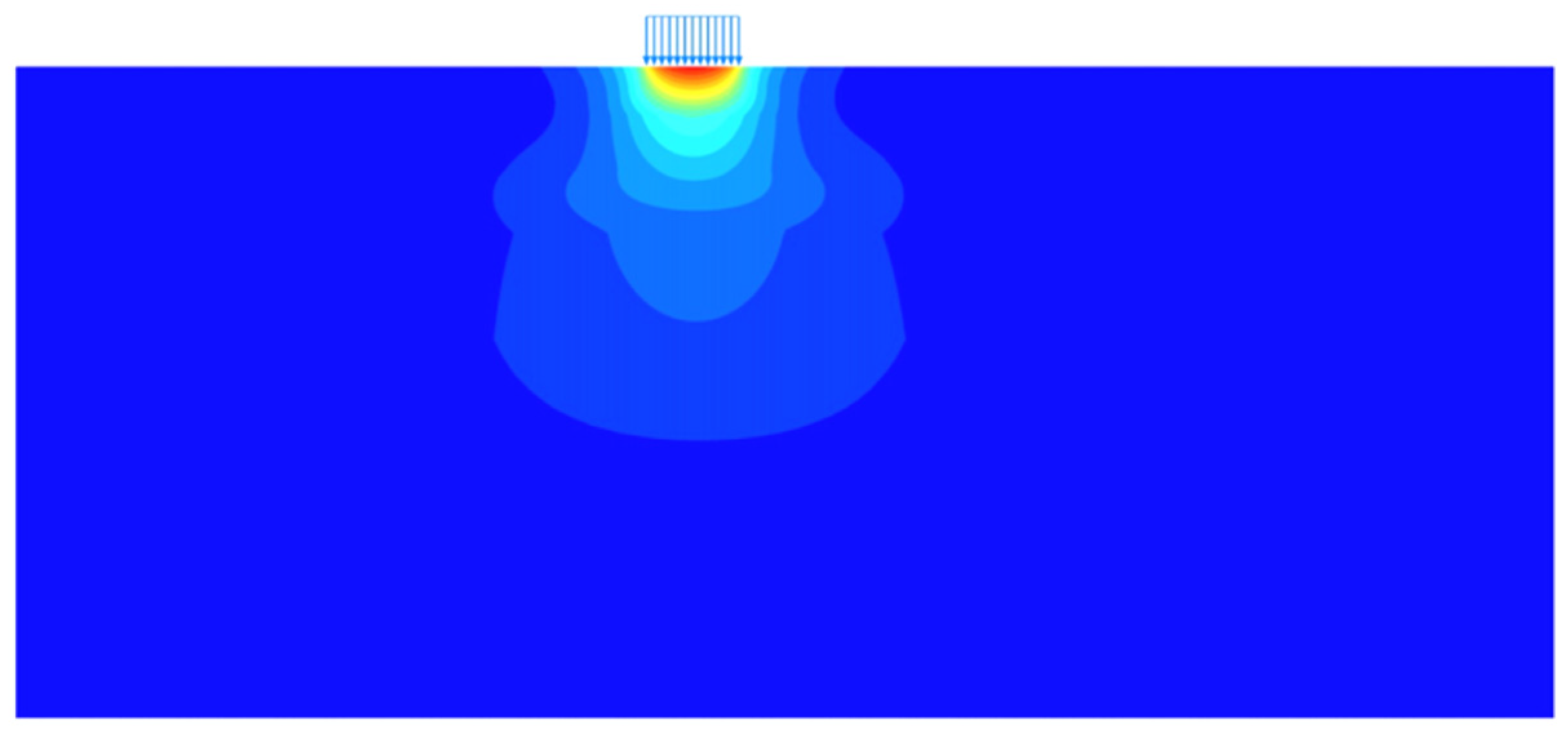
The numerical simulation of the construction process was carried out in strict accordance with the actual construction sequence, which was divided into four steps. Step 1: The upper structural loads were applied and the soil–cement wall (constructed using the pre-installed pile method) was embedded, so as to simulate the initial in situ stress state of the soil and the installation process of the retaining piles. The model configuration at the initial stage is shown in Figure 11.
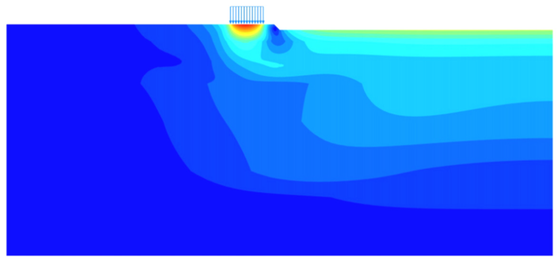
Step 2: The excavation was sloped at a ratio of 1:1 down to 1.0 m below the ground surface, and a shotcrete facing was applied, representing the slope excavation and the initial support installation. The slope excavation stage is illustrated in Figure 12.
Step 3: The excavation advanced to a depth of 1.7 m, at which level a capping beam and one row of anchor cables were installed at the designated positions, simulating the intermediate excavation stage and the corresponding support construction. The excavation and support installation at this stage are shown in Figure 13.
Step 4: The excavation proceeded to the final bottom depth of 6.9 m, while the groundwater level inside the pit was lowered to 7.4 m, modelling the final stage of excavation combined with dewatering. The final excavation stage is depicted in Figure 14.
For each construction step, the simulation incorporated key factors such as soil stress relaxation, changes in support structural forces, and groundwater seepage, thereby ensuring that the numerical model realistically captured the actual field behaviour.

3.4. Analysis of Computational Results

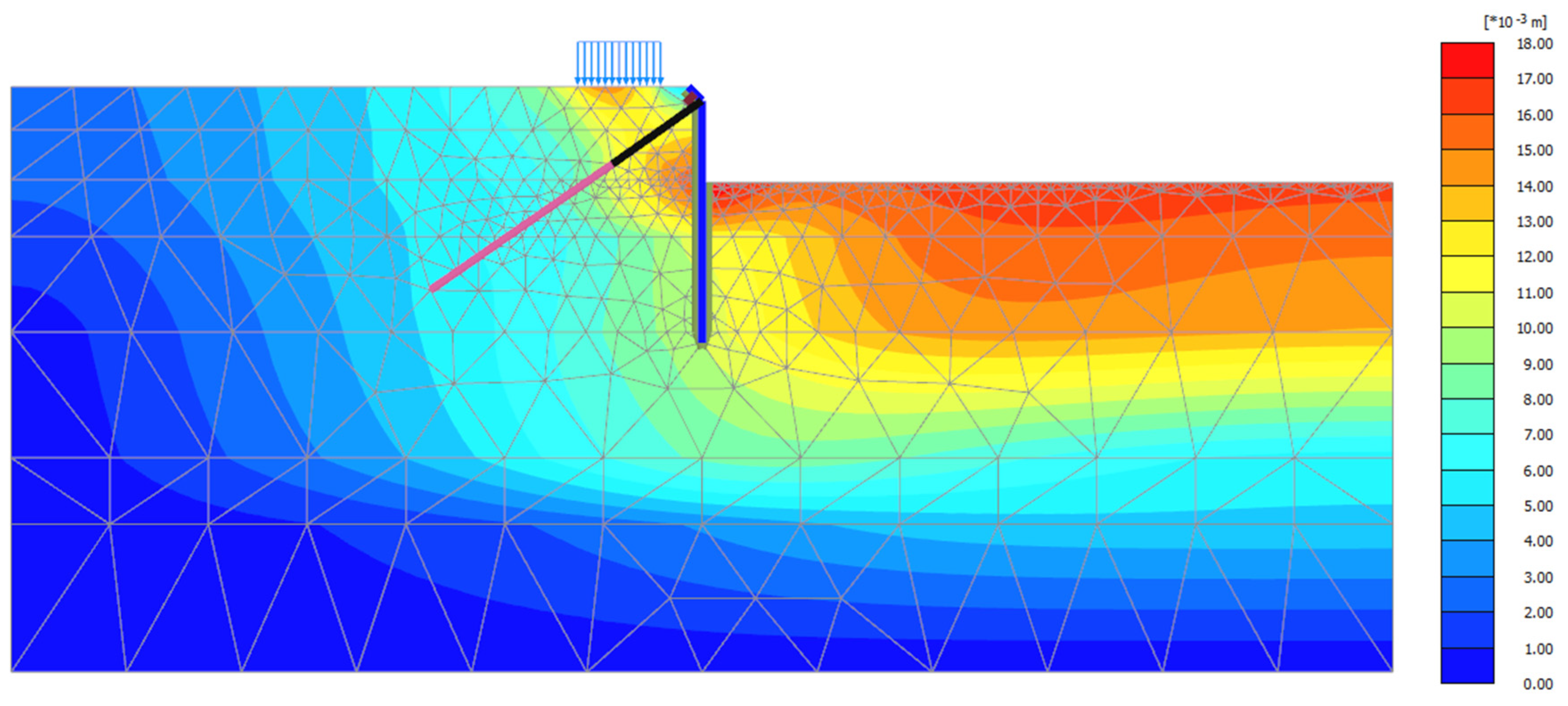
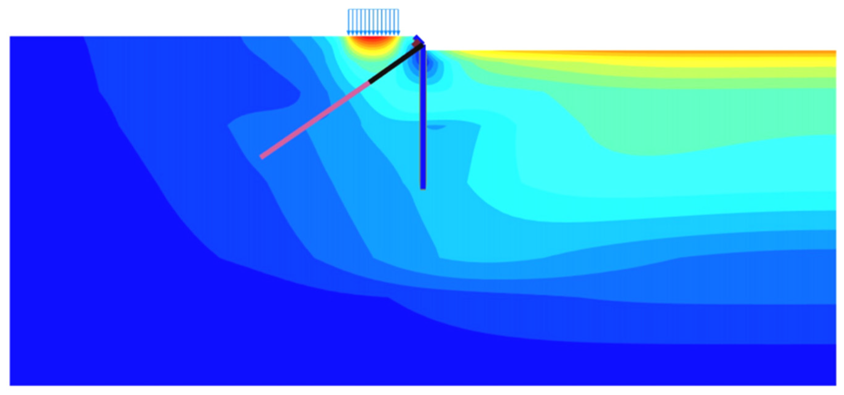
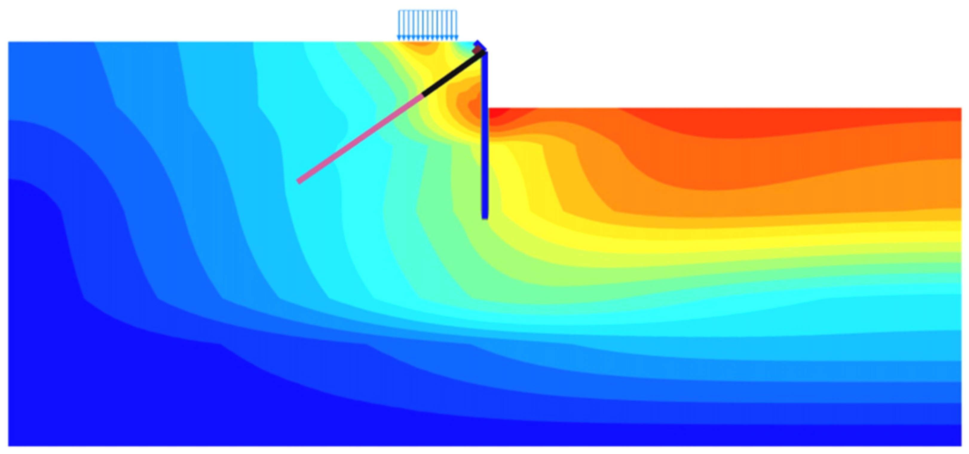
Execution of the finite element model yielded a discretized mesh containing 14,200 nodes. The maximum total displacement recorded across the excavation domain was 17.95 mm, with a maximum horizontal component of 15.95 mm and a maximum vertical component of 16.42 mm. The displacement cloud diagram of the foundation pit support structure is presented in Figure 15. The displacement field exhibited a pattern in which the retaining wall deflected consistently toward the excavation interior throughout the construction sequence, and the deformation magnitude initially increased with depth before attenuating—behavior entirely consonant with the empirically established deformation characteristics of braced excavation support systems.
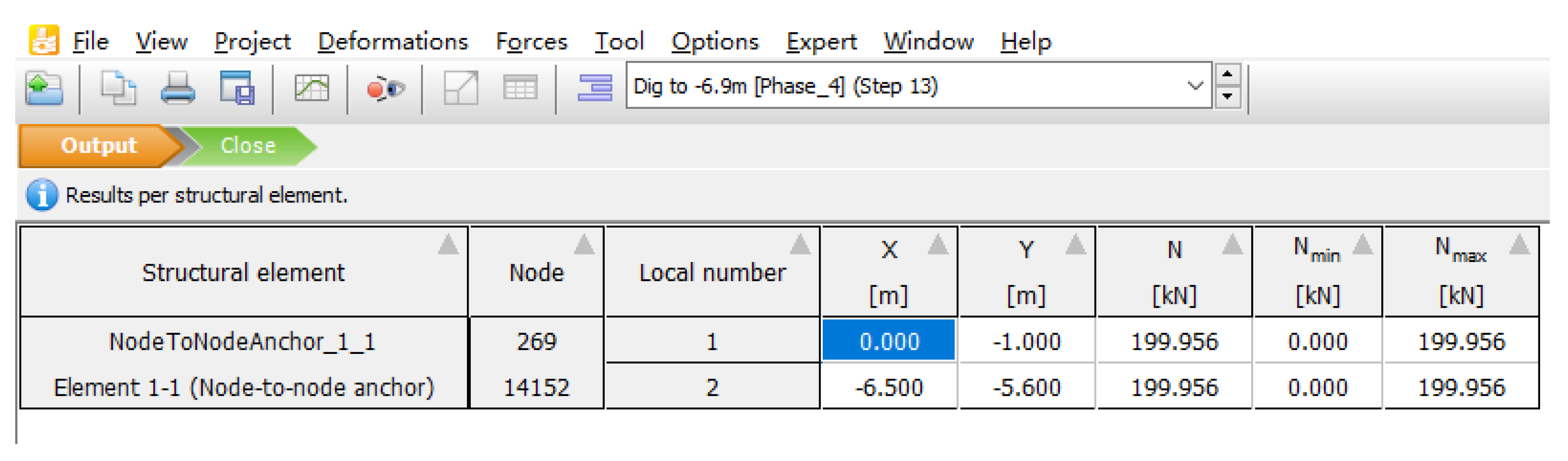
Inspection of the anchor axial forces extracted from the node-to-node anchor elements revealed that at Stage 3, immediately following anchor installation, the predicted force was 150 kN; at Stage 4, when the excavation reached the final formation level, the force rose to 199.227 kN. The axial force calculation results of the node-to-node anchor are shown in Figure 16. This predicted value departs only trivially from the field-monitored stabilized anchor force of 199 kN—well within the tolerance band accepted for engineering purposes—and thus corroborates the fidelity of the finite element model in reproducing the load-carrying behavior of the prestressed anchor.

4. Parametric Sensitivity Analysis

To further elucidate the response of anchor axial force to perturbations in key design parameters and to delineate the degree to which each parameter governs the structural demand on the retaining system, a finite-element-based parametric sensitivity study was undertaken, focusing on three primary factors: anchor embedment depth, excavation depth, and depth to the groundwater table. By varying one parameter at a time while holding all other variables constant, the evolution of anchor axial force was systematically examined across a spectrum of parameter values, thereby permitting identification of the dominant controlling factors. The resulting insights provide a reference framework for the rational selection of anchor design parameters and for the optimized design of deep excavation support systems.

4.1. Influence of Anchor Embedment Depth

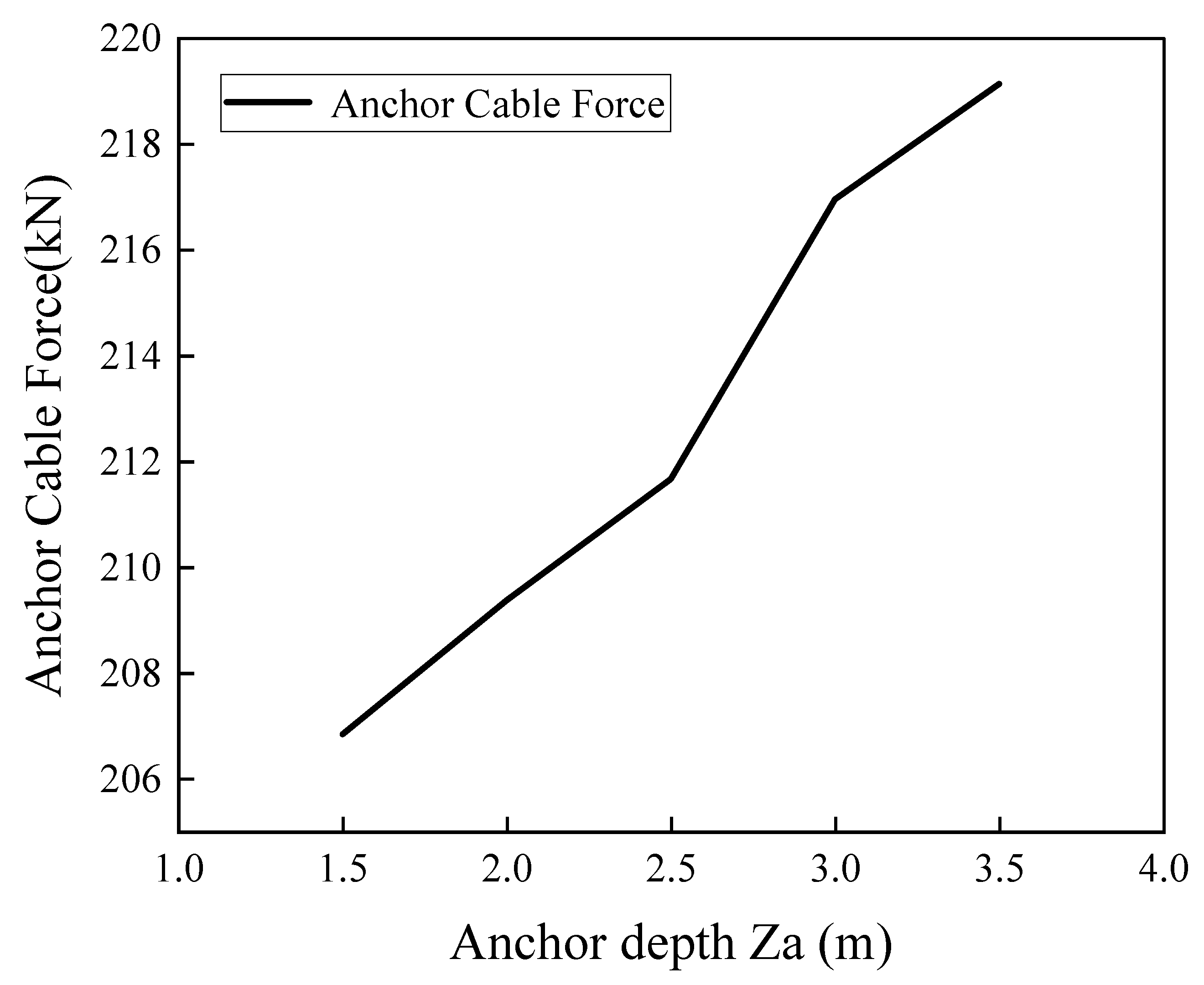
Anchor embedment depth constitutes a readily controllable design parameter whose placement directly governs the magnitude of anchor force and the overall stability of the retaining structure. To resolve the sensitivity of anchor axial force to this parameter, the excavation depth Z d was fixed at 6.9 m, the groundwater table depth Z w at 2.5 m, and the anchor depth Z a was varied through 1.5, 2.0, 2.5, 3.0, and 4.0 m. The results of these simulations are presented in Figure 17.
The analysis demonstrates that anchor axial force exhibits a modest, monotonic increasing trend with greater embedment depth; however, the overall variation is small in magnitude, indicating that while anchor embedment depth exerts a discernible influence, its effect remains comparatively weak. Under the conditions examined, changes in embedment depth had a limited impact on anchor force and did not induce significant fluctuations. Consequently, anchor embedment depth is not the dominant parameter governing anchor axial force variation; its selection should be made with due consideration of the global force and deformation characteristics of the retaining system.

4.2. Influence of Excavation Depth

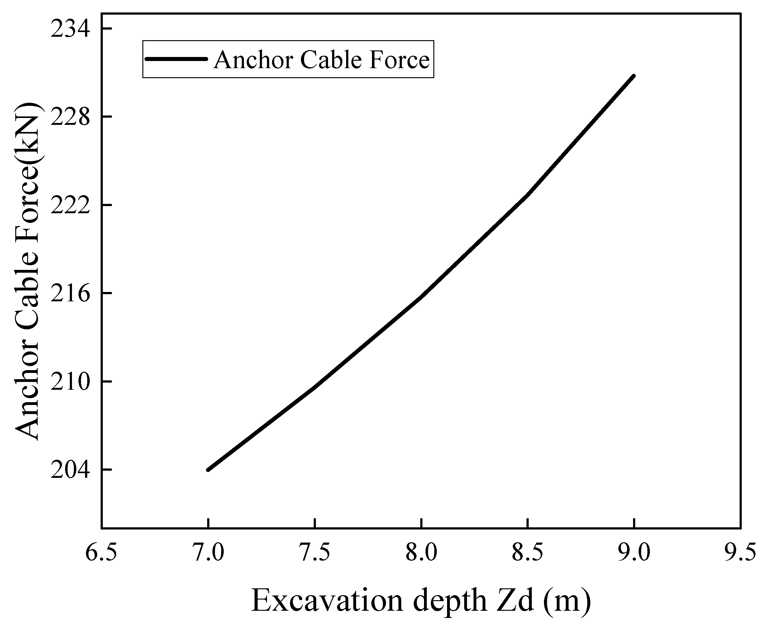
Excavation depth constitutes the cardinal design parameter in deep excavation engineering, and its variation directly modulates both the force demand and the deformation pattern of the retaining structure. To resolve the sensitivity of anchor axial force to this parameter, the anchor depth Z a was held constant at 1.2 m and the groundwater table depth Z w at 2.5 m, while the excavation depth Z d was progressively increased through 7.0, 7.5, 8.0, 8.5, and 9.0 m. The resulting numerical predictions are displayed in Figure 18.
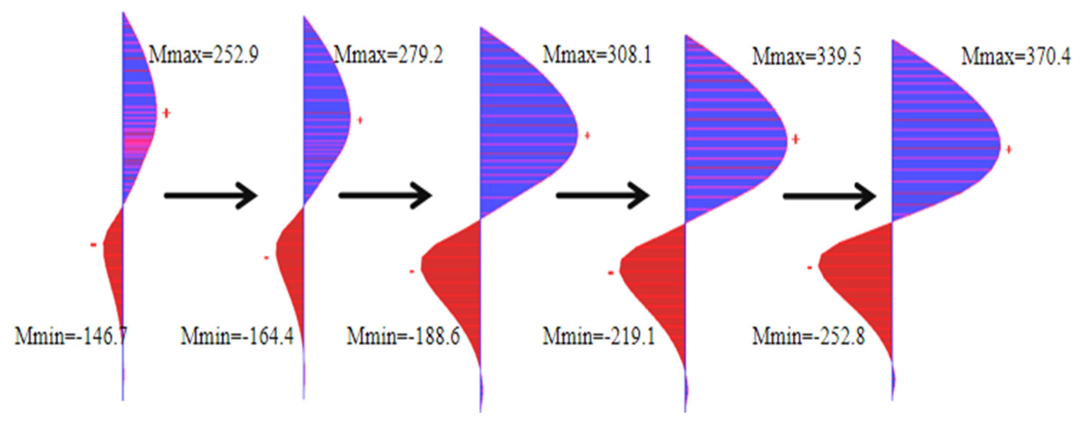
The results demonstrate that anchor axial force escalates continuously and markedly with increasing excavation depth, revealing a pronounced sensitivity. Further interrogation of the bending moment profile along the retaining pile (Figure 19) reveals that the maximum positive bending moment surged by 46.5% and the maximum negative bending moment by 72.3% across the examined depth range. These findings indicate that deepening the excavation not only amplifies the tensile demand on individual anchors but also profoundly reconfigures the internal force distribution within the retaining system. Once the excavation depth exceeds 8.0 m, a single row of anchors proves insufficient to effectively restrain both pile bending moments and lateral displacements; at this juncture, a second—or even multiple—anchor rows should be introduced, commensurate with the moment demand increment and deformation control requirements, to establish a tiered support system that safeguards structural integrity and the stability of the surrounding environment. It is thus evident that excavation depth ranks among the primary determinants of anchor axial force. Consequently, both the excavation depth and the anchor support parameters must be holistically assessed and judiciously selected, with rigorous attention to the integrated structural response and deformation control criteria.
It should be noted that the suggested threshold of 8.0 m for considering multiple anchor rows is primarily based on structural bending moment analysis. In practical engineering design, the final decision must also account for construction feasibility and economic constraints. The introduction of additional anchor rows directly increases material costs (steel strands, anchor heads, grout materials, and fittings), extends construction schedules due to sequential tensioning and testing of multiple rows, and may be constrained by limited working space within the excavation or by the presence of adjacent underground utilities and structures. Therefore, the 8.0 m depth threshold should be regarded as a structural reference guideline rather than an absolute design rule; the final support scheme should be determined through comprehensive consideration of structural safety, construction practicality, and cost-effectiveness under specific site conditions.

4.3. Influence of Groundwater Level Variation

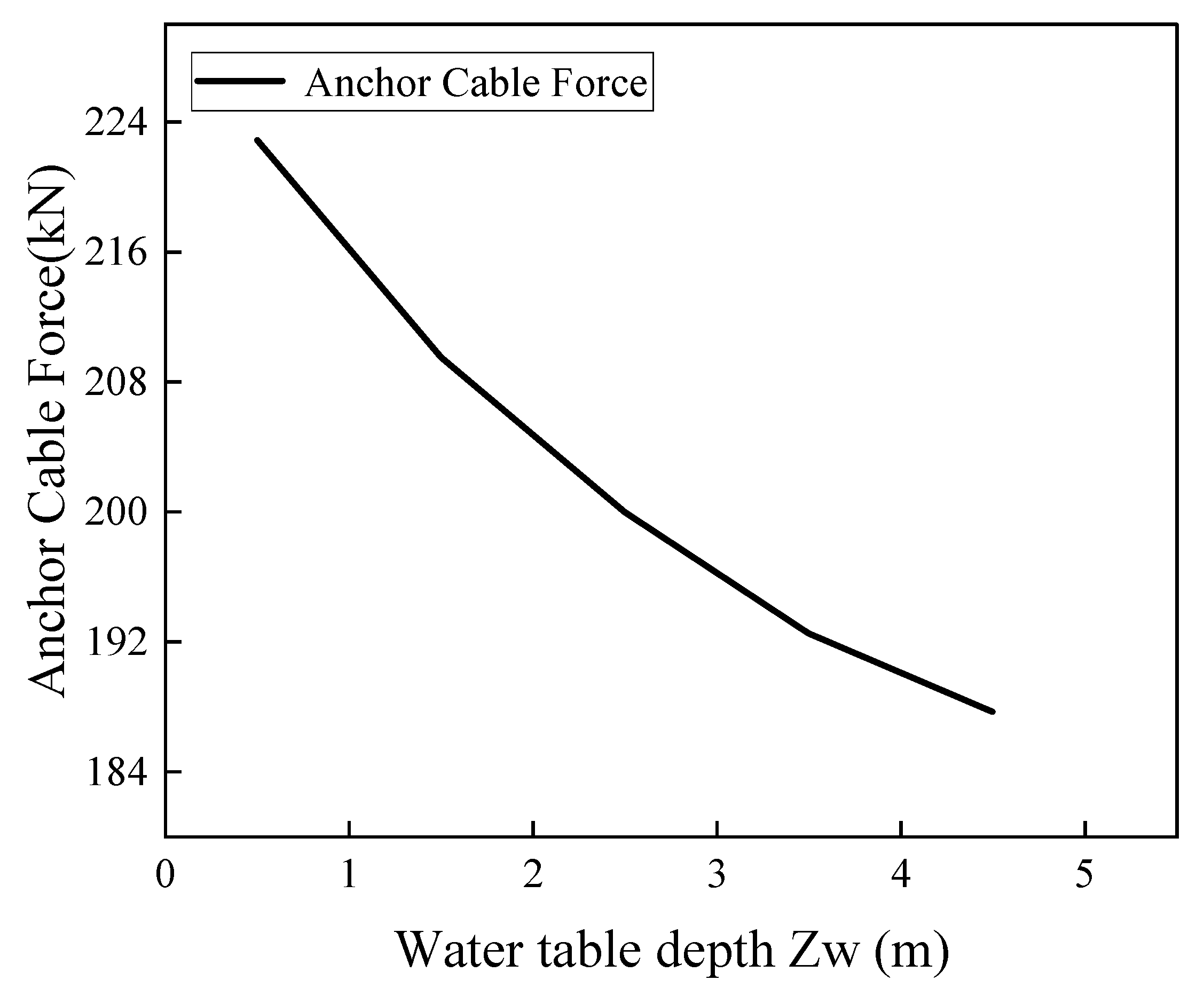
The groundwater table is a decisive environmental factor for excavations in sandy terrain; fluctuations in the water level alter not only the bulk unit weight of the soil but also the effective stress regime and, consequently, the structural demand on the retaining system. To resolve the sensitivity of anchor axial force to this parameter, the excavation depth Z d was fixed at 6.9 m and the anchor depth Z a at 1.2 m, while the depth to the groundwater table Z w was sequentially varied through 3.0, 3.5, 4.0, 4.5, and 5.0 m. The resulting numerical predictions are presented in Figure 20.

5. Conclusions

Based on the theoretical intercomparison, field validation against instrumented monitoring, and finite-element parametric analysis of five anchor axial force prediction methods—the static equilibrium method, the equivalent beam method, the earth pressure envelope method, the chart-based method, and the computed pressure diagram (CPD) method—the following principal conclusions can be drawn within the scope of the specific sandy soil conditions and single excavation case examined in this study:
(1) The various methods yield anchor force predictions that diverge substantially under identical site conditions. In the theoretical benchmark model, the static equilibrium method and the earth pressure envelope method both generated pronounced overestimates—attributable, respectively, to the neglect of pile–soil interaction and to an inherent empirical conservatism—whereas the equivalent beam method, the CPD method, and the chart-based method produced a relatively tight cluster of values, reflecting a shared theoretical rationale for estimating lateral loads in sand.
(2) Benchmarking against field anchor load cell measurements indicates that, for the specific sandy strata encountered in this Hainan excavation, the chart-based method attains the highest accuracy among the methods tested. Its systematic parameter normalization and multi-variate correction framework appears to capture the pile–anchor–soil interaction in sandy strata with greater fidelity.
(3) The finite-element model reproduces the field monitoring data with close agreement, substantiating its reliability for this case. The parametric sensitivity analysis reveals the following: changes in anchor embedment depth exert a weak influence and do not constitute a controlling factor; increasing excavation depth markedly amplifies anchor axial force and profoundly elevates pile bending moments, suggesting that the introduction of multiple anchor rows may be necessary once the excavation exceeds 8.0 m under similar conditions; and a progressively deepening groundwater table drives a monotonic decline in anchor force, implying that regions with a persistently high water table may demand enhanced anchor load-bearing capacity in design.
(4) For analogous pile-anchor retaining structures in comparable sandy soil settings, the chart-based method is suggested as a primary design tool for anchor force estimation, supplemented by finite-element verification of critical construction stages to balance computational efficiency with engineering safety. Design parameters that exhibit strong sensitivity—particularly excavation depth and groundwater level—should be rigorously evaluated, and the support scheme should be judiciously optimized to reflect their influence on structural demand.
Limitations and future work: The findings of this study are derived from a single excavation case in sandy ground conditions in Hainan. The applicability of the chart-based method and the sensitivity trends observed herein to clayey soils, layered deposits, soft ground, different groundwater regimes, or multi-anchor retaining systems has not yet been verified. Future research should incorporate additional field case histories across diverse geological settings, employ more advanced constitutive soil models (e.g., hardening soil or small-strain stiffness models) in finite element analyses, and extend the parametric sensitivity study to include parameters such as anchor inclination, wall stiffness, and anchor spacing.

Author Contributions

Conceptualization, J.H. and M.Z.; methodology, M.Z. and J.L.; software, J.L.; validation, J.L., M.Z. and Z.C.; formal analysis, J.L. and Z.C.; investigation, J.L. and Z.C.; resources, J.H., M.Z. and Z.C.; data curation, J.L. and Z.C.; writing—original draft preparation, J.L.; writing—review and editing, J.H. and M.Z.; visualization, J.L.; supervision, J.H.; project administration, J.H. and M.Z.; funding acquisition, J.H. All authors have read and agreed to the published version of the manuscript.

Funding

This research received no external funding.

Institutional Review Board Statement

Not applicable.

Informed Consent Statement

Not applicable.

Data Availability Statement

The data presented in this study are available on request from the corresponding author. The data are not publicly available due to privacy restrictions.

Acknowledgments

We thank the engineers and technical staff involved in the monitoring work of the Hainan Consulting Design Industrial Base Project for their support in data collection.

Conflicts of Interest

Author Mingsheng Zou was employed by the company Hainan Engineering Consulting and Design Group Co., Ltd. Author Zhangfeng Chen was employed by the company Hainan Design Institute Co., Ltd. The remaining authors declare that the re-search was con-ducted in the absence of any commercial or financial relationships that could be construed as a potential conflict of interest.

Abbreviations

AbbreviationFull Name
CPDComputational Pressure Diagram
SMWSoil Mixing Wall
FEMFinite Element Method

References

  1. Rowe, P.W.; Stroyer; Browzin; Tschebotarioff. Anchored sheet-pile walls. Proc. Inst. Civ. Eng. 1952, 1, 27–70. [Google Scholar] [CrossRef] [Scilit]
  2. Sowers, G.F.; Sowers, G.B. Soil anchors and anchored systems. In Foundation Engineering Handbook, 2nd ed.; Fang, H.Y., Ed.; Springer: New York, NY, USA, 1991; pp. 625–660. [Google Scholar]
  3. O‘Rourke, T.D.; Jones, C.J.F.P. Long-term performance of an anchored sheet-pile wall in stiff clay. J. Geotech. Eng. 1990, 116, 1080–1100. [Google Scholar]
  4. Peck, R.B. Deep excavations and tunneling in soft ground. In Proceedings of the 7th International Conference on Soil Mechanics and Foundation Engineering, Mexico City, Mexico, 1969; State-of-the-Art Report. pp. 225–290. Available online: https://www.issmge.org/uploads/publications/1/38/1969_04_0004.pdf (accessed on 10 May 2026).
  5. Hagerty, D.J.; Nofal, M.M. Design aids: Anchored bulkheads in sand. Can. Geotech. J. 1992, 29, 789–795. [Google Scholar] [CrossRef] [Scilit]
  6. LaCroix, Y.; Atmatzidis, D.K. Design methods for anchored retaining walls. In Proceedings of the 12th International Conference on Soil Mechanics and Foundation Engineering, Rio de Janeiro; Balkema Publishers: Rotterdam, The Netherlands, 1989; pp. 1153–1156. [Google Scholar]
  7. Das, B.M.; Sivakugan, N. Principles of Foundation Engineering, 9th ed.; Cengage Learning: Boston, MA, USA, 2019. [Google Scholar]
  8. FHWA-IF-99-015; Ground Anchors and Anchored Systems. Federal Highway Administration: Washington, DC, USA, 1999.
  9. EN 1997-1:2004; Eurocode 7: Geotechnical Design—Part 1: General Rules. CEN: Brussels, Belgium, 2004.
  10. JGJ 120-2012; Technical Specification for Retaining and Protection of Building Foundation Excavations. China Architecture & Building Press: Beijing, China, 2012.
  11. Bouassida, M.; Porbaha, A. Ultimate bearing capacity of soft clays reinforced by a group of columns—Application to a deep mixing technique. Soils Found. 2004, 44, 91–101. [Google Scholar] [CrossRef] [Scilit] [PubMed]
  12. Li, G.X. Estimating the water and earth pressures on the supporting structure around a foundation pit separately and together. Chin. J. Geotech. Eng. 2000, 22, 348–352. [Google Scholar]
  13. Zheng, G.; Wang, R.Z.; Cheng, X.S.; Lei, Y.W.; Li, X.Y.; Zhou, Q. Mechanism and control of progressive collapse caused by failure of local anchors in multiple-level anchored pile excavation. Chin. J. Geotech. Eng. 2023, 45, 468–477. [Google Scholar] [CrossRef]
  14. Cheng, X.S.; Zhang, R.Z.; Zheng, G.; Wang, R.; Zhang, Y.; Tu, J.; Ma, Y. Experimental study on progressive collapse of tied-back retaining system of excavations induced by partial over-excavation or surcharge loading. Chin. J. Geotech. Eng. 2024, 46, 2078–2088. [Google Scholar] [CrossRef]
  15. Yan, N.; Hao, Z.M.; Bai, X.Y.; Zhang, L.; Sun, L.N.; Zhang, Q.J. In-situ test on force characteristics of miniature pile-anchor-support combination support system for deep foundation pits in miscellaneous soil strata. J. Cent. South Univ. 2024, 55, 755–773. [Google Scholar]
  16. Wang, Z.; Shi, Z.M.; Hou, Z.L.; Zhao, F.; Zhang, Q. Seismic dynamic response and damage mechanism analysis of slope reinforced by pile-anchor structures. Earth Sci. 2025, 50, 3929–3942. [Google Scholar] [CrossRef] [Scilit]
  17. Ding, X.M.; Liu, X.C.; Wang, C.Y.; Ren, J.; Liu, S. Seismic response characteristics of ECC pile-energy dissipation anchor ductile retaining structure. J. Civ. Environ. Eng. 2025, 47, 76–88. [Google Scholar] [CrossRef]
  18. Kumar, P.; Kumar, M.; Chandaluri, V.K.; Sawant, V.A. Uplift capacity of single and group of granular anchor pile system. J. Civ. Eng. Sci. Technol. 2018, 9, 34–40. [Google Scholar] [CrossRef] [Scilit][Green Version]
  19. Zhang, Y.C.; Yang, G.H.; Zhong, Z.H.; Jiang, Y.; Qiao, Y.; Fang, D.; Hu, H.; Liu, P. Discussion on some key problems in soft soil foundation pit design and application analysis of design examples. Chin. J. Rock Mech. Eng. 2012, 31, 2334–2343. [Google Scholar]
  20. Zhou, Y.; Hu, Y.L. Calculation for displacement and internal force of pile anchor retaining structure based on improved increment method. J. Eng. Geol. 2021, 29, 229–236. [Google Scholar] [CrossRef]
  21. Rashid, A.S.; Black, J.A.; Kueh, A.B.H.; Mohamad, H.; Noor, N.M. Bearing capacity charts of soft soil reinforced by deep mixing. Proc. Inst. Civ. Eng.-Ground Improv. 2017, 170, 12–25. [Google Scholar] [CrossRef] [Scilit]
  22. Zheng, H.D. Application Research on Pile-Anchor Retaining Structure for Foundation Pit in Qingdao Soil-Rock Combination Strata. Master’s Thesis, Southwest Jiaotong University, Chengdu, China, 2020. [Google Scholar]
  23. Terzaghi, K.; Peck, R.B. Soil Mechanics in Engineering Practice, 2nd ed.; John Wiley & Sons: Hoboken, NJ, USA, 1967. [Google Scholar]
  24. Jellali, B.; Bouassida, M.; DE Buhan, P. A homogenization method for estimating the bearing capacity of soils reinforced by columns. Int. J. Numer. Anal. Methods Geomech. 2005, 29, 989–1004. [Google Scholar] [CrossRef] [Scilit]
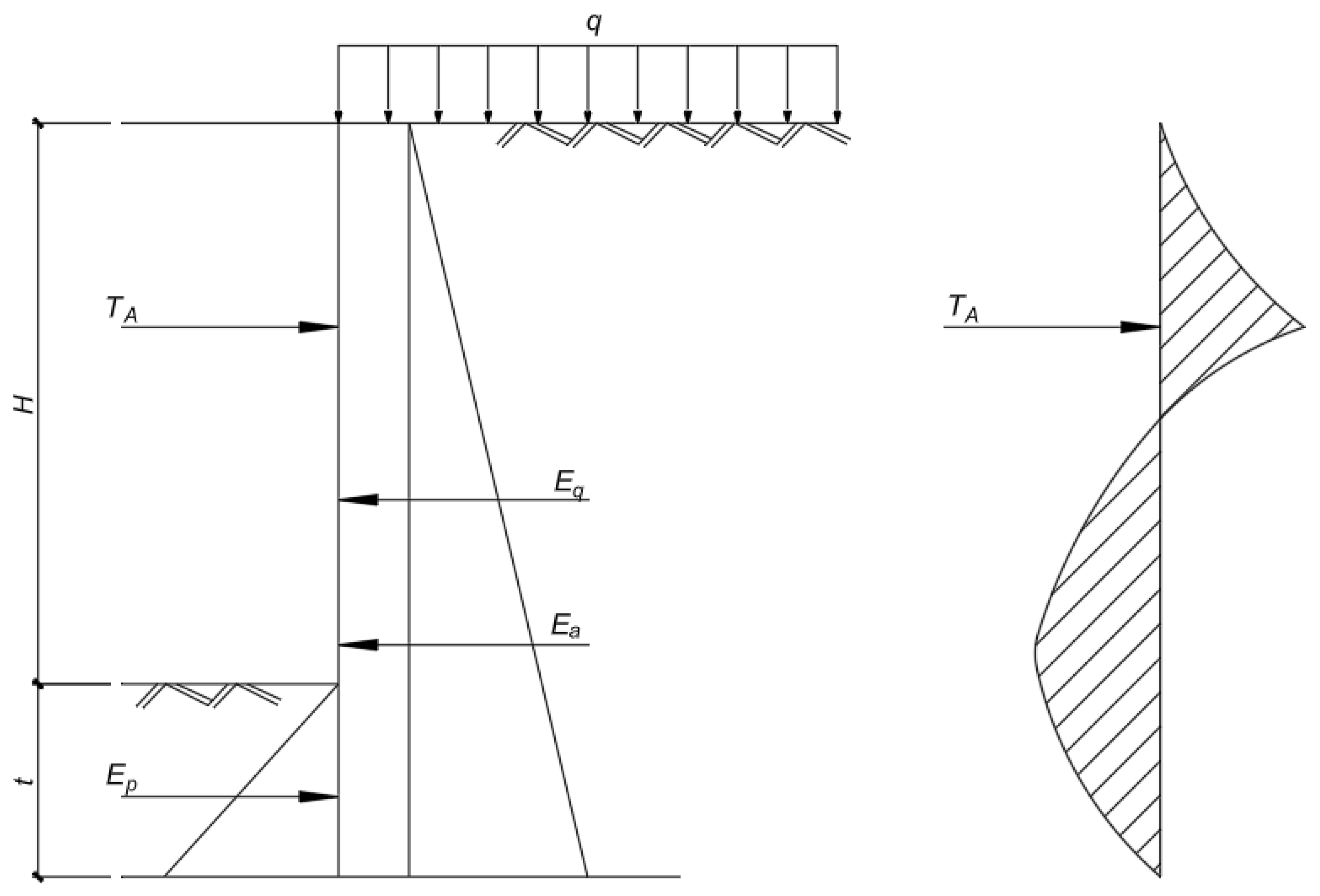
Figure 1. Static equilibrium method.
Applsci 16 08800 g001
Figure 2. Equivalent beam method.
Applsci 16 08800 g002
Figure 3. Force polygon graphical method.
Applsci 16 08800 g003
Figure 4. Schematic diagram of support section for apparent earth pressure envelope method.
Applsci 16 08800 g004
Figure 5. Chart of generalized anchor force vs. anchor depth ratio.
Applsci 16 08800 g005
Figure 6. Chart of water level correction factor vs. anchor depth ratio.
Applsci 16 08800 g006
Figure 7. Support section view of north 3-3 section.
Applsci 16 08800 g007
Figure 8. On-site installation of anchor cable load cell.
Applsci 16 08800 g008
Figure 9. Variation diagram of north side anchor cable axial force.
Applsci 16 08800 g009
Figure 10. Connection diagram of foundation pit support model.
Applsci 16 08800 g010
Figure 11. Connection diagram of initial stage for foundation pit support simulation.
Applsci 16 08800 g011
Figure 12. Connection diagram of slope excavation for foundation pit support simulation.
Applsci 16 08800 g012
Figure 13. Connection diagram of excavation and support construction.
Applsci 16 08800 g013
Figure 14. Excavation to pit bottom.
Applsci 16 08800 g014
Figure 15. Displacement cloud diagram of foundation pit support structure.
Applsci 16 08800 g015
Figure 16. Axial force calculation result diagram of node-to-node anchor.
Applsci 16 08800 g016
Figure 17. Relationship curve of anchor force vs. anchor action depth.
Applsci 16 08800 g017
Figure 18. Relationship curve of anchor force vs. foundation pit depth.
Applsci 16 08800 g018
Figure 19. Variation in pile body bending moment from 7.0 to 9.0 with foundation pit depth.
Applsci 16 08800 g019
Figure 20. Relationship curve of anchor force vs. groundwater level depth.
Applsci 16 08800 g020
Table 1. Apparent earth pressure diagrams by stratum type.
Stratum TypeEarth Pressure DiagramExpressionTotal Earth Pressure
SandRectangular distribution p AEP = 0.65 K a γ H 1.3   ×   Rankine active pressure
Soft–medium clayTrapezoidal distribution p AEP =   K a γ H K a 1.75 × active earth pressure
Stiff clayTrapezoidal distribution p AEP = 0.2 γ H     0.4 γ H Condition: γ H / s u   <   4
Table 2. Correction factors for surcharge anchor force.
φ (°) Z w / Z d Z a / Z d = 0.0 Z a / Z d = 0.1 Z a / Z d = 0.2 Z a / Z d = 0.3 Z a / Z d = 0.4
260.00.9500.9420.9320.9210.909
300.00.9620.9540.9460.9370.926
360.00.9760.9700.9640.9570.949
260.10.8360.8280.8200.8100.799
300.10.8430.8360.8290.8200.811
360.10.8510.8460.8400.8340.827
260.20.7600.7530.7450.7360.726
300.20.7650.7050.7520.7450.736
360.20.7710.7530.7610.7550.749
260.30.7080.7010.6940.6850.676
300.30.7120.7060.7000.6930.685
360.30.7180.7130.7080.7030.697
260.40.6700.6640.6570.6490.640
300.40.6750.6690.6630.6560.649
360.40.6800.6760.6720.6660.660
Table 3. Empirical coefficient table.
Sandy Soil TypeExperience Coefficient C Pressure Ratio R (Passive/Active)Applicable Conditions
Loose sand0.8~0.850.3~0.5Relative density D r   <   35 % , Standard Penetration Test Blow Count N   <   15
Medium-density sandpaper0.7~0.750.55~0.65 35 %     D r     65 % , 15     N     30
Dense sand0.55~0.650.60~0.75 D r   >   65 % , N   >   30
Table 4. Comparison of theoretical calculation results.
Anchor Design Calculation MethodAnchor Axial Force (kN)
Static equilibrium method33.92
Equivalent beam method29.85
Earth pressure envelope method49.47
Chart-based method27.03
Computed Pressure Diagram (CPD) method28.11
Table 5. Physical and mechanical parameters of soil layers.
Layer No.Soil DescriptionUnit Weight γ
(kN/m3)
Cohesion c (kPa)Friction Angle φ (°)Compression Modulus Es
(MPa)
Ultimate Anchor Bond Strength qsk (kPa)
Miscellaneous fill18.0 *10 *12 */20 (primary)/35 (secondary)
Medium sand18.5 *5 *25 *8 *50 (primary)/70 (secondary)
Muddy silty clay17.912.8 (CU)2.9 (CU)2.7330 (primary)/40 (secondary)
Medium sand19.0 *5 *30 *15 *120 (primary)/150 (secondary)
Coarse sand19.5 *5 *35 *18 *150 (primary)/180 (secondary)
Note: Asterisked values are empirically derived.
Table 6. Relative error compared with the field-measured value of 199 kN.
Calculation MethodAxial Force (kN)Relative Error (%)
Equivalent beam method266.4+33.9
Chart-based method200.2+0.6
CPD method239.6+20.4
Table 7. Comparison of calculated values by various theoretical methods and the measured value.
Calculation MethodCalculated Value (kN)Measured Value (kN)Absolute Deviation (kN)Relative Error (%)
Chart-based method200.2199+1.2+0.6
Equivalent beam method266.4199+67.4+33.9
CPD method239.6199+40.6+20.4
Table 8. Mesh sensitivity analysis results.
Mesh SchemeNumber of ElementsNumber of NodesMax. Horizontal Displacement (mm)Deviation from Fine Mesh
Coarse~5200~10,80016.47+6.5%
Medium~9800~19,60015.57+0.7%
Fine~14,200~28,40015.46
Table 9. Convergence criteria adopted in the numerical analysis.
CriterionToleranceDescription
Displacement (absolute tolerance) 1.0 × 10 5 mMaximum displacement increment
Energy 1.0 × 10 3 JDifference between internal and external work
Table 10. Physical and mechanical parameters of soil layers (for numerical simulation).
Layer No.Soil DescriptionUnit Weight γ (kN/m3)Cohesion c (kPa)Friction Angle φ (°)Compression Modulus Es (MPa)Elastic Modulus E (kPa)Poisson’s Ratio ν
Miscellaneous fill18.01012/1.0 × 104 *0.30
Medium sand18.552583.2 × 1040.30
Muddy silty clay17.912.82.92.738.2 × 1030.35
Medium sand19.0530156.0 × 1040.30
Coarse sand19.5535187.2 × 1040.30
Note: * For miscellaneous fill, the elastic modulus was assigned an empirical value owing to the absence of compression-modulus test data. For all other layers, the elastic modulus was converted from the compression modulus using E = 4Es for sandy soils and E = 3Es for cohesive soils. These conversion factors are widely adopted empirical approximations in geotechnical engineering; prior investigations and engineering practice confirm that they adequately represent the deformation characteristics of the ground.
Table 11. Section properties of H-beam (HN700×300×13×24).
ParameterSymbolValueUnit
Cross-sectional area (per beam) A s 231.5cm2
Moment of inertia (strong axis) I s 197,000cm4
Elastic modulus E s t e e l 2.06 × 10 8 kPa
Table 12. Detailed parameters of anchor bond length.
ParameterSymbolValueUnitBasis/Calculation
Grout body diameter d b o n d 0.15mDesign documents
Thickness in ② medium sand h s a n d 4.0mSite investigation
Thickness in ③ muddy silty clay h c l a y 6.0mSite investigation
Ultimate bond strength (② sand) q s k , s a n d 120kPaSite investigation
Ultimate bond strength (③ clay) q s k , c l a y 30kPaSite investigation
Weighted avg. ultimate bond strength q s k , a v g 84kPaThickness-weighted average
Ultimate skin friction per unit length f m a x 39.6kN/m f m a x = q s k , a v g × π × d b o n d
Table 13. Parameters of support structural elements.
Structural ComponentMaterial/TypeAxial Stiffness E A (kN/m)Flexural Stiffness E I (kN·m2/m)Eq. Thickness d (m)Remarks
SMW pile wallHN700×300 steel equivalent 5.29 × 10 6 4.50 × 10 5 1.01Beam spacing 0.9 m
Anchor (free length)4 × Φ15.2 strands 1.092 × 10 5 (per anchor)Node-to-node anchor, 20° inclination
Anchor (bond length)Grout + interfaceEmbedded pile, f m a x = 39.6 kN/m
Disclaimer/Publisher’s Note: The statements, opinions and data contained in all publications are solely those of the individual author(s) and contributor(s) and not of MDPI and/or the editor(s). MDPI and/or the editor(s) disclaim responsibility for any injury to people or property resulting from any ideas, methods, instructions or products referred to in the content.