


Abstract
Deep learning intrusion detectors for IoT networks are mostly evaluated on clean-data accuracy alone, leaving their behavior under perturbation unknown. This paper treats robustness as a tunable design parameter rather than an uncontrolled byproduct. The mechanism itself is not novel, since training with additive input noise penalizes the norm of the input gradient. What is new is its quantified use as an operational control, where one training-time parameter sets a measurable robustness radius. On ToN-IoT and Edge-IIoTset, we evaluate a lightweight CNN-BiLSTM-Attention detector of about 200 K parameters with mutual-information feature selection. Under test-time Gaussian noise and projected gradient descent on modifiable continuous features, clean-data accuracy does not guarantee stability after deployment. A strong random forest, a high-accuracy deep model and a parameter-matched transformer all collapse under small perturbations, so the fragility belongs to the detection task rather than to any model family. Noise-aware training establishes a controllable radius matched to the expected deployment perturbation, retaining about 88 percent accuracy where baselines collapse. It costs clean-data attack recall, which a validation-calibrated threshold restores without reducing robustness, and gradient-free attacks confirm the robustness is genuine. Robustness should therefore be reported alongside accuracy and efficiency as a standard axis for IoT intrusion detection.
1. Introduction
In late 2016, the Mirai botnet compromised hundreds of thousands of poorly secured IoT devices such as cameras and home routers, and used them to launch some of the largest distributed denial-of-service attacks recorded at the time [1]. Mirai was not isolated. Its source code was released publicly, many variants followed, and IoT devices remain both a favored target and a launch point for large-scale attacks [2,3]. With connected devices rising toward tens of billions and attack volumes climbing sharply [4,5], and with such devices typically resource-constrained and infrequently patched, IoT security has become a central concern. Network intrusion detection systems (NIDS) are a primary line of defense, and building detectors that are both accurate and practical is an active problem [2].
Deep learning has driven strong progress in intrusion detection [6], with convolutional, recurrent models such as LSTM, and hybrid models frequently reporting accuracies above 99% on public benchmarks [2,7]. This apparent success can mislead for three reasons that current work addresses only in part. First, most studies report clean-data accuracy alone, yet public datasets are often imbalanced and can contain leakage-prone fields, so a model can score high overall while failing on the minority attack classes that matter operationally. Second, many high-accuracy models are large, conflicting with the constrained gateways on which detection must run. Third, robustness to input perturbation is rarely examined, even though real measurements are noisy and an adversary may deliberately perturb traffic features.
Work published since 2025 has begun to narrow this third gap, with standardized adversarial protocols that test detectors across a range of budgets rather than at one value [8], defenses for resource-constrained models that combine adversarial transfer learning with input smoothing [9], and certified robustness through randomized smoothing adapted to network-traffic feature spaces [10]. What none of it yet provides is a way for an operator to fix the strength of a defense before training rather than discover it afterward, and supplying that control is the purpose of this paper.
This paper reframes IoT intrusion detection around a property that clean-data accuracy cannot capture, namely robustness to input perturbation. Our position is that robustness should be treated not as a fixed, rarely tested attribute of a fielded detector but as a first-class design objective an operator can measure, control, and deliberately set. We make this concrete on ToN-IoT [11] and Edge-IIoTset [5] in binary and multiclass settings, supporting each claim with a mechanistic analysis rather than accuracy numbers alone.
This work makes three contributions.
- Clean-data accuracy does not indicate deployment robustness, and the fragility is a property of the task, not a model family.Under perturbations restricted to modifiable continuous features, as small as 0.5 percent of the range of each feature, both a high-accuracy deep detector and a carefully tuned random forest fail. The random forest collapses consistently to about 0.53 on Edge-IIoTset, below the 0.728 majority-class baseline and worse than a classifier that always predicts the normal class. The deep model is more robust on average but highly unreliable, with accuracy under a fixed perturbation varying by more than thirty points across seeds. A parameter-matched transformer encoder, which shares no structural component with either, fails in the same way. Susceptibility of tree ensembles to constrained adversarial perturbation has been reported before [12]. What has not been done, to our knowledge, is to place a tree ensemble and a deep detector under one identical protocol and to explain their joint failure at the level of where the forest places its split thresholds relative to the attack budget, which Section 4.6.1 does. That explanation rules out an architecture-specific cause and locates the fragility in the sparse, easily perturbed nature of the discriminative features.
- The training-noise level acts as an explicit, tunable robustness radius. Noise-aware training is not itself a contribution of this paper: its equivalence to input-gradient regularization is classical [13], and Gaussian augmentation and randomized smoothing are established techniques [14,15]. What has not, to our knowledge, been made explicit for IoT intrusion detection is the treatment of this mechanism as a measurable control whose output an operator can read before committing to a configuration. A model trained at noise level sigma retains its clean accuracy up to a test-time perturbation of at least sigma, and empirically of at least 1.5× sigma, so sigma becomes a design parameter matched to the expected deployment perturbation. A first-order analysis connects this to a reduction in the input-gradient norm by more than four orders of magnitude against a decision margin that changes by a factor of two, which places the gain in a flattened loss surface rather than in a displaced boundary.
- We quantify the cost of robustness and show it is controllable. Noise-aware training lowers clean-data attack recall at the default threshold, but calibrating the threshold on validation data recovers recall to the standard model’s level while preserving robustness. The choice between a standard and a noise-aware detector thus becomes an explicit, threat-model-dependent deployment decision rather than an unconditional recommendation.
Together, these results argue that robustness belongs alongside accuracy and efficiency as a standard axis for evaluating intrusion detectors. The detector used to establish them is deliberately lightweight, combining mutual-information feature selection with a compact convolution, bidirectional-recurrence, and attention network of about 200 K parameters that runs at roughly 0.08 ms per sample. The same model is therefore both deployable on constrained gateways and the subject of the robustness analysis. We are explicit that the architecture is the vehicle for the study rather than its contribution. Each component adds only a small amount to clean accuracy, and the value lies in the analysis.
2. Related Work
2.1. Deep Learning for Network Intrusion Detection
Early detectors used classical classifiers such as decision trees, SVMs, and random forests over hand-engineered flow features [2,16], and tree ensembles remain strong baselines on tabular traffic data. Deep learning has since become dominant. Convolutional networks exploit local feature or byte correlations [7], recurrent models such as LSTM and GRU capture sequential structure [17], and hybrid convolutional–recurrent architectures combine the two and often outperform either alone [18,19,20,21,22]. Attention and transformer-style models weight the most informative features or time steps [23,24], and several recent detectors combine convolution, bidirectional recurrence, and attention in one pipeline [25]. Our architecture belongs to this hybrid, attention-augmented family. The contribution is not the architecture but its combination with feature selection and, above all, the robustness analysis of Section 4.
2.2. Lightweight and Efficient Detection for the Edge
Because IoT detection often runs on constrained hardware, a growing body of work targets lightweight models through compact architectures [26], separable convolutions, pruning, quantization, and knowledge distillation, typically reporting reductions in parameters, memory, or latency while preserving accuracy. Compact transformer detectors, including quantized encoder models evaluated on Edge-IIoTset itself, now reach competitive accuracy at a footprint suitable for gateway hardware [27], which is why Section Comparison with a Parameter-Matched Transformer compares against a parameter-matched transformer rather than treating the architecture question as settled. Our model is deliberately compact and fast, and we show that feature selection lowers inference latency without materially affecting accuracy. In contrast with most of that literature, we treat robustness as an objective of equal standing with efficiency.
2.3. Feature Selection for Intrusion Detection
Public datasets often contain dozens of features, some redundant, noisy, or leakage-prone, among them identifiers, timestamps, and per-packet quasi-random fields. Filter methods such as mutual information and chi-squared [28], wrapper methods, and embedded tree-based importance are widely used to reduce dimensionality and improve generalization [29]. We use mutual-information selection to quantify how few features are needed rather than to clean the feature set, since the high-cardinality quasi-random fields are removed earlier by the column-level diagnostic of Section 3.3. Performance saturates at a small subset while inference cost continues to grow with the feature count.
2.4. Robustness and Adversarial Machine Learning in Intrusion Detection
Neural networks can be fooled by small, carefully crafted perturbations [30], and projected gradient descent (PGD) is a standard first-order attack and the basis of adversarial training [31], which improves robustness but carries costs including reduced clean accuracy and less stable optimization [32,33]. Several studies adapt such attacks and defenses to intrusion detection, showing that gradient-based perturbations reliably evade deep detectors [34,35], with robust schemes proposed in response [12,36]. A domain-specific constraint is that not every feature can be modified freely: protocol fields, checksums, discrete flags, and identifiers cannot be altered arbitrarily while keeping traffic valid, so credible evaluations restrict perturbations to plausibly modifiable features, typically the continuous ones [34]. Our study follows this principle, perturbing only continuous features with Gaussian noise and PGD. The accuracy–robustness tension is not unique to intrusion detection [37], and training with noise as a route to robustness is well established elsewhere, with the classical equivalence to input-gradient regularization [13] and its role in randomized smoothing [14,15] both taken up in Section 4.6.2. Two points distinguish our analysis. First, we show the fragility extends to a strong random forest, so it is not neural-network-specific. Second, we characterize noise-aware training as a tunable defense, compare it directly against adversarial training (Section 4.6.3), and quantify its cost rather than reporting robustness in isolation.
Three lines of recent work bear directly on this study. The first concerns evaluation methodology. A systematic adversarial assessment of a hybrid convolutional, recurrent, and attention detector constrains perturbations to respect protocol semantics and reports robustness across a range of budgets rather than at one fixed value [8]. That study also finds PGD adversarial training close to cost-free in clean accuracy, which Section 4.6.3 does not reproduce. The two findings are compatible once the scope is noted, since their evaluation stays inside the trained budget whereas ours probes beyond it and also tests Gaussian noise, a regime in which a defense specialized to worst-case gradient directions has no advantage. The second line concerns constrained hardware. A framework combining adversarial transfer learning with differential privacy and data smoothing hardens lightweight tree-based detectors and attributes the gain to reduced sensitivity of the input representation [9], a diagnosis that agrees with ours. What differs is what the operator sees, since their smoothing is fixed in the pipeline whereas the training-noise level studied here is a parameter the operator sets and whose consequence Section 4.6.6 states in advance.
The third line concerns certification and is closest to the claim made here. Randomized smoothing has been adapted to the heterogeneous feature spaces of network traffic, yielding per-record certified radii together with a dimension-level account of which features are certifiable [10]. Certification is a stronger statement than anything offered in this paper and should be preferred wherever its cost is acceptable. Two properties keep it complementary. A certified radius is measured after training, so it reports what was obtained rather than letting an operator specify what is required, and a smoothed classifier draws many noisy samples at inference, whereas the noise layer used here is removed before deployment. The two therefore compose. The training-noise level sets the radius a deployment requires, and certification, where affordable, verifies that the radius was obtained.
2.5. Research Gaps and Positioning
The literature leaves three gaps that map onto our three contributions. First, detectors are overwhelmingly compared on clean-data accuracy, so their behavior under perturbation is unknown. The few studies that evaluate robustness treat it as a fixed property to measure rather than a quantity to control. We show the training-noise level is a tunable robustness radius set to match the deployment threat model (Section 4.6.2 and Section 4.6.6). Second, robustness and efficiency are usually pursued separately. We address both in one lightweight model, and further show that the selected-feature-set size trades off against robustness differently for standard and noise-aware models (Section Feature-Selection Size and Robustness). Third, when robustness is reported, its cost is rarely quantified. We quantify it as a clean-accuracy and attack-recall trade-off and show it is controllable through the decision threshold (Section 4.6.2 and Section 4.6.6). Cutting across all three, the fragility of accurate detectors extends beyond neural networks to a strong random forest, establishing it as a property of the detection task. Table 1 summarizes our position relative to representative prior work.
Table 1.
Positioning of this work relative to representative prior work on learning-based network intrusion detection. NIDS, network intrusion detection system. MCC, Matthews correlation coefficient.
3. Materials and Methods
3.1. Datasets
We evaluate on two recent, widely used IoT datasets, ToN-IoT [11] and Edge-IIoTset [5], each in binary and multiclass settings. ToN-IoT contains network and telemetry data from a realistic IoT/IIoT testbed [38], and we use its network-flow records in full. Such testbeds have become a standard basis for evaluating learning-based detectors [39]. Edge-IIoTset contains traffic from a testbed with more than ten device types. Because the full dataset is large, we draw a stratified 200,000-record sample preserving class proportions. The binary task separates normal from attack traffic, and the multiclass task distinguishes individual attack types plus normal traffic (Table 2). For both datasets, we use a stratified 64/16/20 train/validation/test split, with a fixed seed for reproducibility.
Table 2.
Class composition of the two datasets, given as the number of records and the share of each class in the test partition. The stratified 64/16/20 split preserves these proportions across the training, validation, and test partitions. The binary task groups Normal against all attack classes (Attack). Per-dataset totals and majority-class baselines are stated in the text.
The subsample is drawn with the scikit-learn train_test_split routine, using the label as the stratification key, with shuffling enabled and the random seed fixed at 42. The binary experiments stratify on the binary label and the multiclass experiments on the attack type. We verified this claim empirically rather than assuming it. Under binary stratification, the largest absolute deviation of any class share between the full 2,219,201 records and the 200,000-record sample is 0.0001 percentage points, and a chi-squared goodness-of-fit test against the full-data proportions returns a p value of 0.999 on one degree of freedom. Under multiclass stratification, the largest deviation is 0.0003 percentage points, on the Port_Scanning class, with a chi-squared p value of 1.000 on fourteen degrees of freedom. The two rarest classes survive the draw in proportion, Fingerprinting passing from 1001 records to 90 and MITM from 1214 to 109. Binary stratification alone still holds every multiclass share to within 0.076 percentage points, so the two experimental settings see samples of the same fine-grained composition.
The stratified split preserves the class proportions, so the shares in Table 2 apply to the training, validation, and test partitions alike. The imbalance is substantial: the Normal:Attack ratio is about 1:3.2 on ToN-IoT and about 2.7:1 on Edge-IIoTset in the binary task, while in the multiclass task the largest single class accounts for 23.7% of ToN-IoT and 72.8% of Edge-IIoTset. We therefore report results against the majority-class baseline, defined as the accuracy of a trivial classifier that always predicts the most frequent class. This baseline is 0.763 (binary) and 0.237 (multiclass) on ToN-IoT, and 0.728 (binary and multiclass) on Edge-IIoTset. A detector whose accuracy under perturbation falls below this baseline is worse than a model that ignores its input entirely.
3.2. Data Cleaning and Removal of Identifier Fields
Placeholder missing-value tokens are unified to a common marker and entirely empty columns removed. Fields that identify a host or session, such as IP addresses, timestamps, and address-resolution fields, are removed because they leak identity rather than describe behavior. Remaining missing values are filled with the column median, and all features are min-max scaled to [0, 1]. The scaler is fit on the training split only and applied to validation and test, so no test-set statistics leak into training. As a result, a small fraction of test values may fall slightly outside [0, 1], and these are clipped during the perturbation step (Section 3.7). The same train-only discipline applies to the mutual-information selector (Section 3.4).
3.3. Diagnostic-Driven Feature Engineering
A column-level diagnostic measures, per field, the fraction of unique and of missing values on a 100,000-record sample. Two fields stand out: the per-packet TCP checksum at a unique-value fraction of 0.466 and the raw acknowledgment number at 0.433, which is an order of magnitude above the ephemeral port numbers at 0.062 and several orders above any genuinely behavioral field. They behave like per-packet identifiers that induce overfitting, so they are removed together with the port numbers and the raw hexadecimal payload fields. Sharing a name with a removed field is not itself a reason for removal. The ICMP checksum, for instance, takes a single value across the entire diagnostic sample, so it is an indicator rather than an identifier, which is why it is retained and why it appears among the attack indicator fields of Section 4.6.8. In contrast, several encoded HTTP, DNS, and UDP protocol fields are zero for benign traffic but non-zero under specific attacks. These are genuinely discriminative and retained. Column types are resolved by testing numeric convertibility, so a numeric field containing a non-numeric placeholder is still treated as numeric, and only genuinely categorical fields are label-encoded. For each feature, we record whether it is continuous. This continuous-feature mask later restricts robustness perturbations to features that can plausibly change in real traffic.
3.4. Feature Selection
We apply filter-based mutual-information selection (scikit-learn SelectKBest with the mutual-information score). Mutual information measures the dependence between a feature and the label, is classifier-independent, and captures nonlinear relationships. Features are ranked by mutual information with the label on the training set and the top K retained. The main experiments use all available features. The effect of K is studied in Section 4.5. The main experiments retain all 49 features, so mutual-information selection is inactive there and enters only in the size study of Section 4.5. The name of the model refers to the selection stage being part of the pipeline, not to a reduced feature set being used in the headline results.
3.5. Model Architecture
Three families were candidates for the detector, and the choice among them was driven by the analysis this paper performs rather than by clean accuracy. Tree ensembles are the strongest classical option on tabular flow features and are kept as a baseline in Section 4.3, but they are not differentiable, so they support neither noise-aware training nor the gradient-based diagnosis on which the robustness analysis depends. Graph-based detectors suit lateral-movement campaigns, yet building the graph would reintroduce the address and identity fields that Section 3.2 removes as leakage-prone, and its construction cost falls outside the edge budget targeted here. Transformer encoders are differentiable and would support the same analysis, so Section Comparison with a Parameter-Matched Transformer reports a parameter-matched compact transformer trained under an identical protocol. Convolution followed by bidirectional recurrence was preferred because, on inputs of this length, it reaches higher accuracy at a lower parameter count and roughly half the arithmetic cost.
The model combines convolution, bidirectional recurrence, and self-attention in a compact network (Figure 1). Selected features are treated as a one-dimensional single-channel sequence. Two convolutional blocks (64 and 128 filters, kernel size three, same padding), each followed by batch normalization and ReLU, extract local interactions among neighboring features. Max-pooling with a factor of two and dropout then reduce the sequence length and provide regularization. A bidirectional LSTM with 64 units per direction models dependencies across the feature sequence in both directions. A four-head self-attention layer (key dimension 32) re-weights the sequence toward the most informative positions and is combined with its input through a residual connection and layer normalization. Global average pooling yields a fixed-length representation, which passes through a 64-unit dense layer with dropout and a softmax output sized to the number of classes. The model contains about 199,000 parameters.
Figure 1.
Architecture of the proposed MI–CNN–BiLSTM–Attention model. Mutual-information-selected features are treated as a one-dimensional single-channel sequence. The feature sequence passes through two Conv1D layers with 64 and 128 filters, respectively, each followed by batch normalization and ReLU activation. A single MaxPool1D layer and dropout are applied after the second convolutional layer. The resulting sequence is processed by a bidirectional LSTM with 64 units per direction, followed by four-head self-attention, residual addition, and layer normalization. Global average pooling, a 64-unit dense layer, dropout, and a C-class softmax layer form the classification head. The dashed Gaussian-noise layer is active only during training in the noise-aware variants and is disabled during inference. F denotes the number of selected input features, and C denotes the number of output classes.
3.6. Training Setup
The main experiments use categorical cross-entropy, with a focal-loss option [40,41] for strongly imbalanced settings. Optimization uses Adam (learning rate 0.001, batch size 256) for up to sixty epochs, with early stopping on validation loss (patience fifteen, best-weights restoration) and learning-rate reduction on plateau. A fixed seed is used throughout. Class weighting is not used in the main runs, as it lowered aggregate metrics in preliminary experiments. All experiments ran on a single machine with an Intel Core i7-14700HX CPU (Intel Corporation, Santa Clara, CA, USA).
3.7. Robustness Evaluation and Noise-Aware Training
Robustness is evaluated by perturbing only continuous features, using the mask from preprocessing, since altering categorical or protocol fields would produce invalid or non-functional traffic. Two perturbation types are used. Gaussian noise adds zero-mean noise of increasing standard deviation, with perturbed values clipped to the valid range. Accuracy is measured on a random test subset and averaged over repeated draws. A PGD attack applies seven iterative steps: at each step the input moves a small distance along the sign of the loss gradient, the accumulated perturbation is clipped to an epsilon-ball around the original input, and the result is clipped to the valid range, with the gradient masked so only continuous features are perturbed. Because all features are scaled to [0, 1], a budget epsilon corresponds to a change of at most epsilon per feature, so the budgets used here, 0.005 to 0.05, represent changes of only 0.5 to 5 percent of the range of each feature.
These perturbations act in feature space, and the distinction matters for how the results should be read. Restricting them to modifiable continuous features and bounding them in an L-infinity ball is a proxy for realizability. It does not by itself guarantee that a perturbed record corresponds to valid, functional traffic, which additionally depends on inter-field correlations, count integrality, and protocol semantics. We therefore describe the perturbations as feature-space constrained rather than physically constrained, and interpret the results as robustness to bounded, measurement-scale changes in the features an adversary could plausibly alter. The mask is defined at the level of representation rather than semantics. A field is marked continuous when it is numerically valued after preprocessing, which excludes the label-encoded categorical fields but retains protocol flags that are numerically coded. Section 4.6.7 repeats the evaluation with a mask built on semantic grounds and shows that the conclusion is unchanged.
A further caveat concerns units rather than realizability. A budget of epsilon in the min-max scaled space corresponds to a change of at most epsilon times the observed range of each feature, so for a byte count whose observed range spans several orders of magnitude it amounts to a substantial absolute change near the top of the range and to less than one unit near the bottom. We report budgets in scaled units because the perturbation is applied in the space in which the model operates, and Section 4.6.7 tests directly whether the inter-field correlations mentioned above alter the conclusion.
Noise-aware training inserts a Gaussian noise layer of standard deviation sigma immediately after the input during training only. It is disabled at inference, so it changes what the model learns without changing how it is evaluated. Adding noise forces the model to rely on features that remain informative under perturbation rather than on sparse features a small perturbation can flip. We train variants with sigma = 0.05 and 0.1. The standard model corresponds to sigma = 0.
3.8. Random Forest Baseline and Its Hyperparameter Selection
The random forest serves as a strong baseline, so its configuration was selected rather than assumed. Hyperparameters were chosen by randomized search over 60 candidates, scored by the Matthews correlation coefficient on the fixed validation split so that no test record could influence the choice. The space covered the number of trees at 100, 200, 300, and 500; the maximum depth at unlimited, 10, 20, 30, and 50; the minimum samples required to split a node at 2, 5, 10, and 20; the minimum samples per leaf at 1, 2, 4, and 8; and the features considered per split at the square root of the feature count, its base-two logarithm, 0.3 and 0.5. The seed was fixed at 42, and the search took under two minutes.
The selected configuration uses 500 trees at a maximum depth of 30 with 0.3 of the features per split, reaching a validation coefficient of 0.8135. On the test set, it records an accuracy of 0.9279, a macro-F1 of 0.9001, and a Matthews coefficient of 0.8176, matching the default 100-tree configuration to four decimal places. The ten best candidates share that validation score, while configurations capped at depth 10 fall to about 0.79, so the space was wide enough to separate good settings from poor ones, and the forest is simply insensitive to its remaining hyperparameters once the depth is unrestricted. We therefore keep the 100-tree configuration throughout, and the baseline should be read as a well-tuned forest rather than a default one.
4. Results and Discussion
Three experimental protocols appear in this paper, and the reported values differ slightly between them. The first approach involves a single run on the full test set using a fixed random seed. The second approach reports the mean and sample standard deviation across multiple training random seeds. Specifically, the baseline, ablation, and trade-off experiments use five seeds, while the robustness radius experiments use three seeds. The third approach consists of a single run on a robust subset containing 5000-record, while the measurements for the “expectation-over-transformation” attack were performed on a subset of 2000-record, as the computational cost of this attack is significantly higher than that of the other attacks.
4.1. Overall Detection Performance
Table 3 reports detection performance across both datasets and tasks (Figure S1). Binary detection is strong on both, with near-perfect scores on ToN-IoT and high scores on Edge-IIoTset across accuracy, macro-F1, and MCC. Multiclass is more demanding: it remains strong on ToN-IoT, but on Edge-IIoTset overall accuracy stays high while macro-F1 falls well below it. This gap reflects Edge-IIoTset’s strong class imbalance, in which several attack types have very few samples and are absorbed by dominant classes. We therefore report MCC [42] and macro-averaged precision, recall, and F1 alongside accuracy throughout, since accuracy alone overstates performance under imbalance. Unless noted, each result is a single fixed-seed run. The baseline comparison (Section 4.3) and robustness results (Section 4.6) additionally report the mean and sample standard deviation over multiple seeds.
Table 3.
Overall detection performance of the proposed model on both datasets and both tasks. Macro-Prec., Macro-Rec., and Macro-F1 denote macro-averaged precision, recall, and F1. MCC denotes the Matthews correlation coefficient. Values are from a single fixed-seed run on the full test set.
Figure 2 makes the effect of imbalance concrete. On ToN-IoT, the model detects most classes well, with only a rare class such as password guessing falling to a low F1. On Edge-IIoTset, the frequent classes, including the several DoS variants and normal traffic, are detected almost perfectly, while rare classes such as XSS, uploading, and password attacks are largely missed. The ceiling on multiclass performance is thus set by data scarcity for particular attack types rather than by model capacity, which further motivates imbalance-aware metrics. Confusion matrices for all four experiments are in the Supplementary Material.
Figure 2.
Per-class F1 in the multiclass setting, for ToN-IoT (left) and Edge-IIoTset (right). Bars are sorted by score. Bar shading redundantly encodes the same F1 value as the bar length, with darker shading denoting a higher F1. Frequent classes such as the DoS variants and normal traffic are detected almost perfectly, while several rare attack types receive a low score, showing that data scarcity, not model capacity, limits multiclass performance.
4.2. Model Complexity and Efficiency
Table 4 reports the deployment footprint of the proposed detector and of every architecture compared against it. Floating-point counts depend on how the profiling tool resolves fused kernels, and the profiler used here does not resolve the recurrent cells, so the recurrent contribution is computed analytically as twice the product of the number of directions, the sequence length, four gates, the number of units, and the sum of input channels and units, then added to the profiled remainder. Latency is reported under two protocols rather than one because they differ by more than an order of magnitude, and the difference decides which figure applies to a given deployment. Parameter count and single-precision size need no such qualification and are the two figures that transfer directly to other hardware. Batched latency was re-measured with the profiling harness and differs from the values reported in Section 4.5 by a few percent.
Table 4.
Complexity and deployment footprint. Every measurement was taken on one Intel Core i7-14700HX with no accelerator under TensorFlow 2.21. Floating-point operations are the profiled total plus the analytically computed recurrent contribution, because the profiler does not resolve the fused recurrent kernels. Single-record latency is the median time to classify one record with the inference graph compiled ahead of time. Batched latency is the total time to classify a batch of 256 records divided by the batch size. Values reported by other studies are not tabulated here, for the reasons given in the text.
Latency itself is reported under two protocols that differ by more than an order of magnitude. Single-record latency is the time to classify one record with the inference graph compiled ahead of time, which is what a gateway scoring each flow on arrival experiences. Batched latency divides the time for a batch of 256 records by the batch size, which is what a collector accumulating records experiences. For the full-feature model, the two are 1.33 and 0.084 milliseconds, or about 750 and 11,900 records per second. All timings were taken on one Intel Core i7-14700HX with no accelerator under TensorFlow 2.21, and the batched figure is the one reported in Section 4.5.
Within those limits, the detector is competitive on every transferable axis. It holds 199,234 parameters, occupies 0.76 megabytes, and needs about 10.5 million operations per record at 49 features, of which the recurrent stage accounts for 4.7 million. The count falls to 4.5 million at 20 features and 2.3 million at 10, because every stage scales with the sequence length while the parameter count does not. Peak activation memory is 0.024 megabytes at batch size one, so the whole working set including weights stays under one megabyte. The noise-aware variant is identical to the standard model in parameter count, model size, operation count, and activation memory, because its noise layer is removed at inference. Its measured latency differs by three to eleven percent, which is run-to-run variation on a shared processor rather than a difference in computation, since the two graphs are the same after the noise layer is dropped. Robustness therefore costs nothing at deployment. Its entire price is paid at training time and in clean-data recall, and both are quantified in Section 4.6.2. That division matters when the alternative is considered. Adversarial training runs an inner attack loop at every optimization step, costs roughly an order of magnitude more to train, and buys a narrower robust range, as Section 4.6.3 shows.
4.3. Comparison with Baseline Methods
Table 5 compares the model with five baselines under identical preprocessing, feature selection, data splits, and (for deep baselines) training budget (Figure S2). Every value is the mean over five seeds with sample standard deviation. The baselines are a pure 1D CNN, a pure bidirectional recurrent network, a convolutional–recurrent hybrid without attention, a parameter-matched compact transformer, and a random forest. The proposed model outperforms all four deep baselines on every metric. A well-tuned random forest is a strong competitor and slightly exceeds our model on clean data, with accuracy of 0.928 against 0.923 and MCC of 0.818 against 0.804. On tabular network-flow features, tree ensembles remain highly competitive, yet this small clean-data advantage does not translate into reliability after deployment. As Section 4.6 shows, the random forest is no more robust than our model once inputs are perturbed, so clean-data accuracy is an incomplete measure of which model to trust in the field.
Table 5.
Comparison with baseline methods on Edge-IIoTset (binary). MCC denotes the Matthews correlation coefficient. Parameter counts are given for the neural models. For the random forest, the ensemble size is reported, since tree models have no directly comparable parameter count. All values are the mean and sample standard deviation over five seeds. The compact transformer is a parameter-matched encoder baseline described in Section Comparison with a Parameter-Matched Transformer, with a model dimension of 112, two pre-norm blocks and four attention heads, trained under the same protocol, splits and seeds as every other row.
Comparison with a Parameter-Matched Transformer
Because attention-based detectors are the most visible alternative to convolutional–recurrent hybrids, we trained a compact transformer encoder to the same parameter budget. It embeds each feature into a model dimension of 112, adds a trainable position embedding, applies two pre-norm blocks of four-head self-attention with a feed-forward width of 192, and reads out through global average pooling and the same classification head, giving 201,842 parameters against 199,234. Preprocessing, feature selection, splits, optimizer, training budget, and the five seeds match every other row of Table 5.
On clean data, the transformer is slightly but consistently weaker, at accuracy 0.9193, macro-F1 0.8871 and a Matthews coefficient of 0.7949 against 0.9227, 0.8924 and 0.8038. Paired tests across the five seed-matched runs give differences of 0.34 accuracy points with a 95 percent confidence interval from 0.05 to 0.63 and a p value of 0.031, of 0.89 points on the Matthews coefficient at a p value of 0.026, and of 0.52 points on macro-F1 at a p value of 0.038. The gap is small but resolvable, unlike the attention effect of Section 4.4, and it runs against the transformer despite its larger parameter count. Even the hybrid without attention, using a third fewer parameters, exceeds it by 0.22 accuracy points, although that difference is not resolvable at a p value of 0.253.
The efficiency comparison is less ambiguous. Self-attention over 49 positions costs about 20.4 million operations per record against 10.5 million for the proposed model, and batched latency follows at 0.149 against 0.084 milliseconds on the same machine. The quadratic term of self-attention is not the difficulty at this length. The cost comes from projecting every position into a model dimension of 112 in both blocks, whereas the proposed model pools the sequence to 24 positions before its recurrent and attention stages run, so contracting the sequence early is the cheaper route to this accuracy.
The more consequential result concerns robustness. Under standard training, the transformer fails exactly as the other architectures do. Accuracy under noise of standard deviation 0.1 falls to 0.7332, which is 18.6 points below its clean value and only 0.5 points above the 0.728 majority-class baseline, so the model has largely collapsed onto the dominant class. Under a PGD budget of 0.02 it averages 0.469 and ranges from 0.341 to 0.625 across seeds, reproducing the unreliability documented in Section 4.6.1. Training the same encoder at sigma equal to 0.1 removes the failure, holding 0.8738 under noise and 0.8755 under attack over three seeds with standard deviations of 0.002 and 0.001, for paired gains of 13.8 points at a p value of 0.007 and 41.7 points at a p value of 0.009, against a clean-accuracy cost of 3.72 points. These paired differences are computed within the three seeds common to both arms and are therefore not equal to the difference of the five-seed and three-seed means quoted above. Three seeds suffice for this arm because it is a replication and its across-seed spread is very small.
Two conclusions follow. Architecturally, a convolutional–recurrent hybrid is the better choice at this input length and parameter budget on both accuracy and cost. Substantively, and this is what matters for the paper, the fragility of Section 4.6.1 and its removal by noise-aware training reproduce on a model that shares no component with the proposed one beyond the classification head. A pure attention encoder and a convolutional–recurrent hybrid collapse under the same perturbations, are rescued by the same intervention, and converge to almost the same robust accuracy, 0.874 against 0.878. Taken with the failure of the random forest in Section 4.6.1, this places the fragility in the detection task rather than in any family of models.
4.4. Ablation Study
We evaluate four variants on Edge-IIoTset (binary): BiLSTM only, CNN only, the convolutional–recurrent hybrid, and the full model with attention, with corresponding rows in Table 5 and mean ± sample SD over five seeds (Figure S3). The recurrent-only model is weakest (accuracy 0.900) and by far the most variable across seeds (SD 0.011 in accuracy, 0.032 in MCC), since treating the features as a single sequence offers limited local structure. The convolutional model is stronger and much more stable (0.914), the hybrid reaches 0.921, and the full model reaches 0.923.
Adding attention changes accuracy by 0.12 points on average across the five seeds, with a paired standard deviation of 0.27 points. Rather than rest the claim on overlapping error bars, we test it. A paired t-test on the seed-matched runs gives t equal to 1.00 on four degrees of freedom, a p value of 0.375 and a 95 percent confidence interval from minus 0.21 to plus 0.45 accuracy points, and the corresponding tests on the Matthews coefficient and macro-F1 give p values of 0.372 and 0.377 with intervals that also contain zero. The attention module therefore produces no effect this experiment can resolve. The phrasing is deliberate, because five seeds give a paired test limited power and the signed-rank test cannot fall below 0.0625 at this sample size, so what is defensible is that any effect of attention is smaller than the run-to-run variability of training. The same protocol resolves the random forest advantage of 0.51 accuracy points easily, returning t equal to 10.19 at a p value of 0.0005 with an interval from plus 0.37 to plus 0.65, which is what licenses the negative conclusion about attention rather than a mere absence of evidence.
Convolution and recurrence together account for essentially all of the clean-data performance, while attention adds capacity without a measurable accuracy benefit. Whether any component instead contributes robustness is the question Section Component Contribution to Robustness addresses.
Component Contribution to Robustness
Section 4.4 shows that no component produces a reliable clean-accuracy gain. Whether any produces a robustness gain instead is the question here, so we repeated the ablation under perturbation. Each of the four variants was trained under both regimes across the same five seeds and evaluated under Gaussian noise with a standard deviation of 0.1 and under PGD at a budget of 0.02. Table 6 reports the mean and sample standard deviation over the seeds, together with the clean-accuracy cost of noise-aware training as a paired difference within each variant and seed.
Table 6.
Component ablation under perturbation on Edge-IIoTset (binary), mean and sample standard deviation over five seeds. Accuracy under noise is measured at a test-time Gaussian standard deviation of 0.1 and accuracy under attack at a PGD budget of 0.02, both on the 5000-record robustness subset. Clean-accuracy cost is the paired difference in clean accuracy between the noise-aware and the standard run of the same variant on the same seed, in percentage points. All values in this table come from a dedicated set of training runs performed for the robustness ablation.
Under standard training, no variant is robust, and none is reliably more robust than another. Accuracy under noise spans 17.9 points, from 0.540 for the full model to 0.719 for the hybrid, and accuracy under attack spans 35.5 points, from 0.310 to 0.665, while the across-seed standard deviations reach 0.19 and 0.32, so the ordering carries no information. A paired test confirms this. Attention changes accuracy under noise by minus 17.9 points with an interval from minus 42.7 to plus 6.9 at a p value of 0.115, and accuracy under attack by minus 27.3 points with an interval from minus 65.5 to plus 10.9 at a p value of 0.118, so it buys neither clean accuracy nor robustness. The clearest evidence is the instability of the direction itself. The paired effect on clean accuracy is plus 0.12 points in the runs behind Table 5 and minus 0.13 points in the independent runs behind Table 6, with both intervals containing zero. The second value is computed from those runs but is not tabulated, since Table 6 reports only the robustness columns and the paired cost.
Under noise-aware training, the picture inverts. The three variants containing a recurrent stage land within 0.1 points of one another in every column, the convolution-only variant sits about 1.3 points below them, and the spread across architectures falls from 17.9 to 1.4 points under noise and from 35.5 to 1.3 points under attack. The across-seed standard deviation falls to about 0.004 everywhere, so averaged over the four architectures the spread is 25 times smaller under noise and 48 times smaller under attack. Paired improvements range from plus 15.8 to plus 33.8 points under noise and from plus 21.3 to plus 56.8 points under attack, against a clean-accuracy cost that stays between 3.4 and 4.5 points whichever components are present, and all twelve comparisons remain significant at the five percent level after Holm correction. The training regime therefore dominates the architecture by more than an order of magnitude on the robustness axis, and both its benefit and its cost belong to the training procedure rather than to the network. Table 7 collects the paired comparisons used throughout this paper.
Table 7.
Paired comparisons across seed-matched training runs on Edge-IIoTset (binary). Differences are in percentage points. Confidence intervals are two-sided at 95 percent from a paired t-test with four degrees of freedom, except for the two transformer noise-aware rows, which are paired over three seeds and therefore have wider intervals. Cohen’s dz is the standardized paired effect size. The first four rows come from the runs behind Table 5 and the next five from the independent runs behind Table 6, which is why the same comparison appears with opposite sign on clean accuracy. Every comparison with a p value below 0.05 survives Holm correction across the number of tests performed.
4.5. Effect of Feature-Selection Size
We vary the number of mutual-information-selected features from 10 to 49 (all features) on Edge-IIoTset (binary). Table 8 reports the results (Figure S4). Performance rises steeply to about 20 features and then saturates: with only 10 features the model already reaches 92.1% accuracy, 0.3 points below the full-feature model, and beyond 20 features differences fall within training variability. Mutual-information selection thus identifies a compact, highly informative subset, with most remaining features redundant for binary detection. The parameter count stays at 199,234 regardless of how many features are selected, so the benefit of selection appears entirely in per-record computation and in preprocessing. Table 4 quantifies the reduction as a fall from 10.5 to 2.3 million floating-point operations between 49 and 10 features, and the latency in Table 8 follows from 0.083 to 0.044 milliseconds per record. A smaller, faster feature set can thus be used at almost no cost in detection quality.
Table 8.
Effect of the number of mutual-information-selected features on Edge-IIoTset (binary). Inference time is measured per sample. Values are from a single fixed-seed run on the full test set.
Feature-Selection Size and Robustness
The feature count has little effect on clean accuracy but a pronounced effect on robustness that depends on the training method. We repeat the robustness evaluation for 10, 20, and 49 features under standard and noise-aware training on the same test subset as Section 4.6, reporting accuracy under PGD at a representative budget of 0.02 (Table 9, Figure S5).
Table 9.
Robustness under a PGD attack at a budget of 0.02 for models trained with different numbers of selected features (K), on Edge-IIoTset (binary). Values are accuracy on the robustness evaluation subset. sigma denotes the standard deviation of the noise added during training.
For the standard model, robustness decreases sharply as the feature set grows. Accuracy under attack falls from 0.56 (10 features) to 0.55 (20) to 0.20 (49), with the same trend at other budgets. Since clean accuracy is essentially unchanged, the features beyond the compact high-information subset do not contribute robustness. Instead, they enlarge the attack surface with more of the sparse, easily perturbed cues identified in Section 4.6.1. For a standard model, a smaller, higher-information feature set is therefore not only cheaper but more robust. For the noise-aware model, robustness is high and almost flat across all three sizes (0.83 at 10 features to 0.87 at 49), so noise-aware training largely decouples robustness from feature count, and an operator can use the full set for its slightly higher clean accuracy without losing robustness.
These results refine the efficiency argument of Section 4.5. For a standard model, reducing the feature count improves both efficiency and robustness at almost no clean-accuracy cost. For a noise-aware model, the feature count mainly trades a small amount of clean accuracy while robustness stays high. In both cases, the full-feature standard model is the least robust configuration despite its high clean accuracy, reinforcing the paper’s central finding at the level of feature selection.
4.6. Robustness and the Accuracy–Robustness Trade-Off
Section 4.1, Section 4.2, Section 4.3, Section 4.4 and Section 4.5 evaluate models on clean test data. This section examines robustness. We diagnose the fragility of accurate models under perturbation, show how noise-aware training removes it and at what cost, compare against adversarial training, replicate on ToN-IoT and in the multiclass setting, rule out gradient masking with gradient-free attacks, characterize the tunable robustness radius and the recovery of attack recall, test whether perturbation models that respect the empirical correlation structure alter the conclusion and whether a semantically defined perturbation mask changes it, examine adaptive attacks and direct field manipulation, and set out the procedure by which an operator selects the training-noise level. Unless stated otherwise, perturbations affect only continuous features and Edge-IIoTset (binary) is the primary case. To separate training-seed from evaluation variability, the trade-off results (Table 10, Figure 3) are the mean and sample standard deviation over five seeds, the adversarial-training comparison (Table 11) is a representative single run, and the radius results (Table 12) are the mean and sample standard deviation over three seeds. Figures tracing accuracy across budgets likewise show a representative single run.
Table 10.
Accuracy–robustness trade-off on Edge-IIoTset (binary), mean and sample standard deviation over five seeds. Clean Acc. is clean-data accuracy. Attack Recall and Attack Prec. are the recall and precision of the attack class on clean data. The last three columns give accuracy under test-time Gaussian noise of the stated standard deviation, applied to continuous features. sigma denotes the standard deviation of the noise added during training. The random forest is non-differentiable, so it does not appear in the PGD panel of Figure 3. For reference, the majority-class baseline, which always predicts the majority Normal class, is 0.728 on this dataset, so a model whose accuracy under noise falls below 0.728 is worse than that trivial classifier. Unstructured Gaussian noise is the weakest perturbation considered in this paper and already drives the forest to 0.53, below the majority-class baseline, so a search-based attack could only lower it further.
Figure 3.
Accuracy–robustness trade-off on Edge-IIoTset (binary), mean and sample standard deviation over five seeds. (Left), accuracy under test-time Gaussian noise for the standard model, two noise-aware models (sigma = 0.05 and 0.1), and a random forest, with error bars of one standard deviation across seeds. (Right), accuracy under a PGD attack at a budget of 0.02. The random forest is non-differentiable, so this attack is not applicable. The noise-aware models stay high with small error bars, the random forest collapses consistently to about 0.53, and the standard model is not only lower on average but highly variable.
Table 11.
Comparison of noise-aware training with adversarial training on Edge-IIoTset (binary), a representative single run. The adversarially trained model uses a training-time PGD budget of 0.03 with seven inner steps. Acc. @ noise gives accuracy under test-time Gaussian noise. PGD gives accuracy under a PGD attack at the stated budget.
Table 12.
Robustness radius as a function of the training-noise level sigma, on Edge-IIoTset (binary), on the 5000-sample robustness subset, mean and sample standard deviation over three seeds. r(sigma) is the largest test-time Gaussian-noise level at which accuracy stays within five points of the clean value. The asterisk marks a lower bound set by the extent of the tested noise grid (0 to 0.3).
4.6.1. Fragility of Accurate Models Under Perturbation
High clean accuracy does not imply robustness. Table 10 and Figure 3 report the accuracy–robustness trade-off over five seeds. Both accurate models lose most of their accuracy under a small perturbation, but differently. The random forest collapses consistently, from 0.928 clean to about 0.53 under Gaussian noise (SD below 0.02 across seeds), below the 0.728 majority-class baseline, so under perturbation it is worse than a trivial classifier that always predicts the normal class. The standard deep model is more robust on average but far less reliable, because its accuracy under noise of 0.1 averages 0.64 yet ranges from 0.39 to 0.73 across seeds, and under a PGD budget of 0.02 averages 0.29 yet ranges from 0.07 to 0.69. In its most fragile runs, the collapse is severe: Figure 4 shows a representative run where accuracy falls from 0.924 clean to 0.06 under PGD at a budget of only 0.01, a change of just 1 percent of each feature’s range, and stays far below its clean value at every larger budget. That a strong random forest fails the same way locates the cause in the detection task rather than a model family, consistent with prior reports that tree ensembles are susceptible to constrained adversarial perturbation [12].
Figure 4.
Accuracy under a PGD attack applied to continuous features, for the standard model and the noise-aware model trained at sigma = 0.1, on Edge-IIoTset (binary), a representative single run. The horizontal axis is the perturbation budget epsilon. The standard model collapses, dropping to about 0.06 at a budget of 0.01, while the noise-aware model stays near 0.87 across all tested budgets.
The shared cause lies in the nature of the discriminative features. Many attack indicators here are sparse fields, zero for benign traffic and non-zero under attack. For the deep model, a decision boundary on such a feature is highly sensitive to a small perturbation that makes a zero-valued cue appear active, producing many false positives. The random forest fails for the same reason. Its trees split on the same sparse indicators, and a hard threshold is crossed as soon as a small perturbation makes a zero-valued field slightly positive, flipping many predictions at once. A model that depends on these sparse cues therefore achieves high clean accuracy but has almost no margin against perturbation, whether neural network or tree ensemble.
We make the argument about the forest quantitative. Of the 49 continuous features, 45 hold a single value on most records and turn non-zero only under particular attacks. Across the ensemble, they carry 51.3 percent of the impurity importance and 40.2 percent of the permutation importance, so roughly half the forest’s discriminative power sits on features that are almost constant. More directly, the ensemble places 3136 splits on them at a median threshold of 0.0179, and 1646 of those splits, or 52.5 percent, fall below the attack budget of 0.02. A perturbation inside the budget therefore crosses more than half the thresholds the forest has learned on these features, and because the thresholds recur across trees, one perturbation flips many trees at once, which accounts both for the abruptness of the collapse and for its reproducibility across seeds.
The effect concentrates where the forest relies most. Among the sparse features with the largest permutation importance, tcp.len carries 1204 splits at a median threshold of 0.0036 with 82.4 percent below budget, udp.stream 172 splits at 0.0002 with 86.6 percent, http.content_length 134 splits at 0.0003 with 82.1 percent, and udp.port 102 splits at 0.0006 with 92.2 percent. The protocol flags behave in the opposite way, since arp.opcode and the four TCP connection flags carry 143, 144, 98, 82, and 66 splits at median thresholds at or above 0.5 and none of them is reachable within the budget. Figure 5 shows the two populations separating on either side of the budget, which identifies the near-zero indicators rather than the flags as the carrier of the fragility.
Figure 5.
Mechanism of the random forest’s collapse on Edge-IIoTset (binary). (Left), the fifteen features receiving the highest permutation importance, with the impurity-based importance shown alongside, each labeled “continuous” or “sparse near-binary”, and with the median split threshold printed next to every sparse feature. Each feature is labeled as either ‘continuous’ or ‘sparse near-binary’, and the median segmentation threshold is indicated next to each sparse feature. Sparse indicators hold 51 percent of the impurity importance and 40 percent of the permutation importance across the full feature set. (Right), one point for each sparse indicator feature, positioned by its median split threshold and the number of splits it receives across the ensemble, with color and marker size giving the fraction of that feature’s splits falling below the attack budget. The dashed line marks the budget of 0.02 and the shaded region marks the thresholds a perturbation within the budget can cross. Of the 3136 splits placed on sparse indicators, 1646 lie inside that region.
The two model families fail on the same class of features but not on the same individual features. The Spearman correlation between the deep model’s input-gradient saliency and the forest’s permutation importance is minus 0.05, and minus 0.004 against impurity importance, so the rankings are unrelated. That is informative rather than contradictory, and it sharpens the claim. The fragility is not caused by one field both classifiers happen to trust but by a property shared across a large group of fields, namely that their discriminative information lies within a band of the range narrower than the perturbation budget. Any classifier that extracts that information inherits the vulnerability, whichever members of the group it uses.
Section 4.6.8 tests the same mechanism on the deep model directly and shows that writing a single indicator field lifts its false-positive rate on normal traffic from 0.1 percent to 72.7 percent. That section also reports a negative control in which the same sparse fields, ranked by input-gradient saliency instead of by their association with the label, leave the false-positive rate at zero. Saliency in a model that treats features as a one-dimensional sequence therefore reflects position within the sequence as much as reliance on the field, which is a caution for saliency-based interpretation in this domain and the reason the analysis above is anchored in the data. The same collapse appears once more in a parameter-matched transformer encoder, which loses 18.6 accuracy points under noise of standard deviation 0.1, and varies by 28 points under attack across five seeds, before noise-aware training restores it to within 0.4 points of the proposed model’s robust accuracy, as Section Comparison with a Parameter-Matched Transformer reports.
The contrast is one of reliability as much as average performance. Across seeds, the noise-aware models vary by at most 0.03 in accuracy under noise and the random forest by under 0.02, whereas the standard model varies by up to 0.15 under Gaussian noise and 0.23 under PGD, so whether a given trained instance is robust is close to chance. This is consistent with the mechanism above, because a standard model’s robustness depends on which sparse cues a particular run happens to weight. This spread is a property of training, not evaluation. Resampling the 5000-example robustness subset five times without retraining changes accuracy by at most 0.008. A standard model that happens to be robust therefore cannot be distinguished from a fragile one at training time, which is an operational liability in itself. Noise-aware training removes exactly this uncertainty.
4.6.2. Noise-Aware Training and the Quantified Trade-Off
Noise-aware training removes this fragility. By adding Gaussian noise during training, the model is forced to discount the sparse, easily perturbed cues and rely on features that remain informative under perturbation. Averaged over five seeds (Table 10, Figure 3), the noise-aware models retain about 0.87 accuracy across a wide range of test-time Gaussian noise, against about 0.53 for the random forest and about 0.64 (with large seed-to-seed variance) for the standard model. The same benefit extends to adversarial perturbation: under PGD, the noise-aware model stays near 0.875 across budgets while the standard model collapses (Figure 4). Over five seeds, its accuracy under a budget of 0.02 is 0.879 ± 0.004 against 0.291 ± 0.233 for the standard model. Noise-aware training thus improves robustness to both random and gradient-based perturbations, even though only random noise is used in training.
The training-noise level behaves as a tunable robustness radius. A model trained at sigma keeps its clean accuracy up to a test-time perturbation of at least sigma, after which it declines. Across our range, the radius is about 1.5–2.1× sigma, quantified on Edge-IIoTset. The model trained at 0.05 retains 0.856 at test noise 0.1 and 0.704 at 0.2. The model trained at 0.1 remains at 0.841 even at 0.2. Because the two variants incur almost the same clean-accuracy cost, sigma can be chosen to match the expected deployment perturbation without an additional accuracy penalty. Figure S6 shows the same trade-off as a heat map.
The gain has a clear mechanistic explanation. Figure 6 compares the input-gradient saliency of the standard and noise-aware models, defined as the mean absolute gradient of the predicted-class probability with respect to each feature. For the standard model, saliency is large and uneven, dominated by one continuous feature and many sparse, near-binary attack indicators, consistent with the fragility of Section 4.6.1, since a large input gradient means a small perturbation produces a large output change. Noise-aware training reduces the saliency of essentially every feature, lowering the mean absolute gradient of the predicted-class probability with respect to the input by roughly three orders of magnitude, from 15.8 to 0.008. This quantity and the median L1 norm of the logit-margin gradient reported in Figure 7 measure the same phenomenon at different levels: the first taken on the predicted-class probability and averaged over features and the second on the logit margin and summed over features, and both fall by three to four orders of magnitude under noise-aware training. Adding input noise during training therefore acts as gradient regularization, which is equivalent to a penalty on the input-gradient norm [13], and flattens the decision surface so that no small perturbation, random or adversarial, moves the output far. This mechanism is well established and underlies the interpretation of adversarial examples as test error under noise [14] and randomized-smoothing certificates [15]. We use it not as a novel defense but as a controllable one. It also connects to explainable intrusion detection, where methods such as SHAP identify the features driving decisions [43,44], surveyed in recent work on explainable AI for cybersecurity [45].
Figure 6.
Input-gradient saliency of the standard and noise-aware models on Edge-IIoTset (binary), for the twelve highest-saliency features in the standard model, on a logarithmic scale. Saliency is the mean absolute gradient of the predicted-class probability with respect to each feature. Features are labeled continuous (cont.) or sparse near-binary (sparse). Noise-aware training lowers the mean saliency across all features by about three orders of magnitude, from 15.8 to 0.008, which flattens the decision surface and explains the robustness gain.
Figure 7.
Mechanism of the tunable radius on Edge-IIoTset (binary), measured on the 5000-record robustness subset. (Left), the median L1 norm of the input gradient of the logit margin on a logarithmic left axis and the median decision margin on a linear right axis, both as functions of the training-noise level. The gradient falls by more than four orders of magnitude while the margin falls by a factor of two and then plateaus. (Right), the first-order predicted radius, defined as the median ratio of margin to gradient norm, together with the measured robustness radius and the reference line at which the radius equals the training-noise level, all on a logarithmic axis. The shaded band is the interquartile range of the first-order prediction across records. The two radii differ in absolute scale because the first-order expansion is local and the logit margin is inflated by softmax saturation, so the comparison establishes that they rise together rather than that they coincide.
A first-order expansion makes this quantitative. For a record whose logit margin is m, an L-infinity perturbation of size epsilon can change that margin by at most epsilon multiplied by the L1 norm of its input gradient, so the perturbation at which the prediction can first flip is approximately m divided by that norm. Evaluating both quantities on the 5000-record robustness subset for sigma from 0 to 0.20 gives Figure 7. For the standard model, the median margin is 3.85, and the median gradient L1 norm is 1.51 times ten to the fourth, which predicts a radius of 0.0014. The smallest budget used anywhere in this paper, 0.005, exceeds that radius by a factor of 3.6 and the representative budget of 0.02 by a factor of 14.6, which is why the standard model does not survive even the mildest perturbation tested and why its collapse is abrupt.
Across the same range, the median gradient L1 norm falls from 1.51 times ten to the fourth to 0.86, a factor near seventeen thousand, while the median margin falls only from 3.85 to 1.89 and is flat above sigma equal to 0.05. The gain therefore comes from flattening the loss surface around the data rather than from displacing the decision boundary, which is the quantitative form of the gradient-regularization mechanism identified above. The predicted radius rises from 0.0014 to 2.20 and the measured radius from 0.0027 to 0.30. The two do not coincide, because the logit margin is inflated by softmax saturation and a first-order expansion holds only locally, and what the comparison establishes is that both rise together across the tested range, so the tunable radius of Section 4.6.6 has an identified cause.
Robustness has a measurable cost. As Table 10 shows, noise-aware training reduces clean-traffic attack recall from 0.72 (standard) to 0.64 (sigma = 0.05) and 0.57 (sigma = 0.1), so between 36 and 43 percent of attacks go undetected on clean data at the default threshold. This cost grows modestly with sigma but is not intrinsic: it is a property of the default 0.5 threshold and is recovered in Section 4.6.6. The mechanism is the one that causes fragility. A model taught to distrust sparse attack cues becomes more conservative and leans toward the benign class. The noise-aware models retain very high attack precision (about 0.98), so an alarm is almost always correct. The practical consequence is a threat-model-dependent choice: a trusted, low-noise environment can use the standard model for higher clean accuracy and recall, while a noisy or adversarial environment can use the noise-aware model for stability under perturbation. Calibrating the threshold on validation data recovers recall to the standard model’s level while preserving robustness (Section 4.6.6).
4.6.3. Comparison with Adversarial Training
Since adversarial training is the standard defense against gradient-based attacks [31], we ask whether noise-aware training is genuinely good or merely cheap. We trained a Madry-style PGD adversarially trained model of identical architecture (training-time budget 0.03, seven inner steps) and compared it against the standard and noise-aware models on the same grid (Table 11 and Figure 8, a representative single run).
Figure 8.
Robustness of the standard, adversarially trained (PGD, epsilon = 0.03), and noise-aware (sigma = 0.1) models on Edge-IIoTset (binary). (Left), accuracy under test-time Gaussian noise. (Right), accuracy under PGD. Adversarial training matches noise-aware training under PGD within its trained budget but collapses beyond it (at 0.05) and is markedly weaker under Gaussian noise, whereas noise-aware training remains robust to both across the tested range.
Noise-aware training compares favorably on three counts. First, robustness beyond the trained budget. Adversarial training matches the noise-aware model under PGD within its trained budget (0.883 at 0.02, 0.913 at 0.03) but collapses to 0.280 once the budget exceeds its training value (0.05), where the noise-aware model holds 0.874. Adversarial training thus buys robustness up to a fixed radius but does not generalize beyond it. Second, robustness to random noise. Specialized to worst-case gradient-shaped perturbations, adversarial training is markedly weaker under Gaussian noise, retaining 0.725 and 0.730 at noise 0.1 and 0.2 against 0.872 and 0.832 for the noise-aware model. Third, cost. Adversarial training carries an inner attack loop at every step and is roughly an order of magnitude more expensive to train, at comparable clean accuracy (0.883 vs. 0.875).
We report this as a scoped comparison rather than a claim of general superiority. The adversarially trained model here is a single standard Madry-style configuration trained on adversarial examples alone at a fixed budget and evaluated on one run, and a more elaborate scheme that mixes clean and adversarial examples, uses a TRADES-style objective, or trains over a range of budgets could recover clean accuracy or widen its robust range. A recent evaluation of a hybrid detector reports exactly that outcome, finding PGD adversarial training to be close to cost-free within its trained budget [8], which is consistent with the pattern observed here once the budget is not exceeded. Within these bounds, the pattern is clear. Against a standard adversarial-training baseline at a fixed budget, noise-aware training provides broader, budget-agnostic robustness to both random and gradient-based perturbations at a fraction of the training cost, making it the more favorable point on the cost–robustness frontier for resource-constrained IoT deployment. The two are complementary, and combining them is a natural extension (Section 5).
4.6.4. Replication on ToN-IoT and Extension to the Multiclass Setting
We test the generality of the analysis along two axes: a second dataset and the multiclass task.
Repeating the procedure on ToN-IoT (binary), the pattern replicates (Figure 9). The standard model reaches 99.4% clean accuracy but loses more than half under a PGD budget of 0.02 (accuracy 0.49), dropping to 0.25 at 0.05, and falls to 0.73 under Gaussian noise of 0.2. The noise-aware model stays at or above 0.91 under every PGD budget and every noise level, at a clean-accuracy cost of about six points (0.994 to 0.934). The standard model is more resilient here than on Edge-IIoTset at the smallest budgets, consistent with ToN-IoT binary being an easier task, but the qualitative conclusion is unchanged: high clean accuracy again fails to guarantee robustness, and noise-aware training again closes the gap.
Figure 9.
Replication of the robustness analysis on ToN-IoT (binary). (Left), accuracy under a PGD attack as a function of the budget epsilon. (Right), accuracy under test-time Gaussian noise as a function of the noise standard deviation sigma. In both panels, the standard model degrades under perturbation, while the noise-aware model (sigma = 0.1) stays high, reproducing the pattern observed on Edge-IIoTset.
The pattern also holds in the multiclass setting, where the detector must identify the specific attack type and macro-F1 is more informative because it is not dominated by the majority class. We evaluate standard and noise-aware models on both datasets, reporting accuracy and macro-F1 under Gaussian noise and PGD on the 5000-example robustness subset, so clean values differ slightly from Table 3 (Figure 10 and Figure S7). On Edge-IIoTset, the standard model’s clean macro-F1 of 0.61 collapses to about 0.06 under noise 0.1 and under a PGD budget of 0.02, while its accuracy stays near 0.71, essentially the 0.728 majority-class baseline, because the model has effectively collapsed to predicting the dominant normal class. This is a stark illustration of why accuracy alone is misleading. The noise-aware model retains a macro-F1 near 0.29 and accuracy near 0.86 across the same perturbations. On ToN-IoT, the standard model’s clean accuracy 0.82 and macro-F1 0.73 fall to 0.39 and 0.30 under noise 0.1, whereas the noise-aware model holds accuracy near 0.57 and macro-F1 near 0.51. The cost of noise-aware training is larger in the multiclass setting, most visibly as a lower clean macro-F1 on Edge-IIoTset (0.30 against 0.61) and lower clean accuracy on ToN-IoT (0.59 against 0.82). This reflects the same conservatism that lowers binary attack recall. The qualitative conclusion is unchanged on both axes: the standard model’s clean performance does not survive perturbation, while noise-aware training preserves a stable, if lower, level. The accuracy–robustness trade-off and its control through the training-noise level are therefore properties of the detection task, not artifacts of a single dataset or the binary setting.
Figure 10.
Multiclass robustness on Edge-IIoTset, on the 5000-example robustness subset. Accuracy (solid) and macro-F1 (dashed) for the standard and noise-aware (sigma = 0.1) models under test-time Gaussian noise (left) and PGD (right). The standard model’s macro-F1 collapses under a small perturbation while its accuracy is propped up by the dominant classes. The noise-aware model retains a stable, lower macro-F1.
The higher multiclass cost is partially recoverable at no cost to robustness. A per-class decision bias calibrated on the validation set to maximize macro-F1, a post hoc logit adjustment held fixed and then evaluated on the test set, raises the noise-aware model’s clean macro-F1, on the full test set, from 0.53 to 0.61 on ToN-IoT, which closes about 40 percent of the gap to the standard model, and from 0.29 to 0.33 on Edge-IIoTset. Figure 11 and Figure S8 are drawn on the 5000-record robustness subset, so the values there are about one point higher. The recovery holds under Gaussian noise and introduces no adversarial fragility: under PGD both the default and calibrated decision rules remain robust (Figure 11 and Figure S8). It is only partial, because a post hoc adjustment cannot restore classes the noise-aware model has learned to ignore. On Edge-IIoTset, several rare attack types are missed outright, capping the achievable macro-F1, so a residual multiclass cost remains, and reducing it through class-balanced or recall-oriented noise-aware training is a natural next step. This refines rather than overturns the binary result: the clean-performance cost of noise-aware training is controllable in both settings, fully recoverable in the binary case (Section 4.6.6) and partially recoverable in the multiclass case. In both cases, robustness is preserved.
Figure 11.
Recovery of multiclass macro-F1 on Edge-IIoTset for the noise-aware model (sigma = 0.1), on the 5000-example robustness subset. Macro-F1 under test-time Gaussian noise (left) and PGD (right), under the default argmax decision and under a per-class decision bias calibrated on the validation set. The dotted line marks the standard model’s clean macro-F1. Calibration raises macro-F1 across the noise range without introducing adversarial fragility, but the gain is capped by rare attack classes the noise-aware model has learned to ignore.
4.6.5. Gradient-Free Attacks Rule out Gradient Masking
A defense that sharply reduces input-gradient magnitude can appear robust to gradient-based attacks without being robust in fact. This failure mode is known as gradient masking, or obfuscated gradients [46]. Two of its signatures are present here: the noise-aware model’s accuracy under PGD is almost insensitive to the budget (Figure 4 and Figure 9), and its input-gradient saliency is about three orders of magnitude smaller than the standard model’s (Figure 9). We therefore verify the robustness is genuine. Because the Gaussian-noise layer is active only in training and disabled at inference, the evaluated model is deterministic. This is not a randomized defense, so expectation-over-transformation does not apply to the deployed model, and the appropriate diagnostics are stronger white-box attacks together with gradient-free black-box attacks.
We evaluate the standard and noise-aware models on Edge-IIoTset (binary) under five attacks (Figure 12). These are the seven-step PGD of the main text, a stronger variant with fifty steps and ten random restarts, a transfer attack whose adversarial examples are crafted on the undefended standard model (which has large, usable gradients) and evaluated on the noise-aware model, and two gradient-free black-box attacks, SPSA and a random-search Square-style attack. At a representative budget of 0.02, the noise-aware model retains 0.875 under every attack, including 0.874 under both gradient-free attacks, essentially identical to the gradient-based attacks, and the transfer attack likewise leaves it at 0.875. The standard model collapses under all five to a worst-case accuracy of 0.028.
Figure 12.
White-box, transfer, and gradient-free attacks on the standard and noise-aware models (Edge-IIoTset, binary) at a perturbation budget of 0.02. For the noise-aware model, the gradient-free black-box attacks (SPSA and random search) achieve accuracy essentially identical to white-box PGD, and a transfer attack from the undefended standard model also fails, which rules out gradient masking. The standard model collapses under every attack.
As a sanity check, at a large budget of 0.30, the same attacks, including the gradient-free ones, drive the noise-aware model down to between 0.12 and 0.14, well below every trivial baseline (majority-class 0.728, all-attack 0.272, chance 0.5), and drive the standard model to zero. This has two implications. First, the attacks are effective and correctly implemented, so the noise-aware model’s stability at small budgets is not merely a failure to attack. Second, the robustness is a bounded radius rather than invulnerability. The model resists small perturbations and yields to large ones, exactly as the tunable-radius account predicts. That the gradient-free attacks are no more successful than the gradient-based ones rules out gradient masking and indicates that noise-aware training genuinely flattens the decision surface in a neighborhood of the data.
One scope limitation remains. Our threat model is bounded, measurement-scale perturbation of the modifiable features, including both benign sensor noise and an adversary restricted to small feature-space changes, rather than an unconstrained worst-case attacker. For that model, the combination of a stronger white-box attack, a transfer attack from an undefended model with usable gradients, two gradient-free black-box attacks, and the large-budget sanity check is the appropriate level of scrutiny, and all agree the robustness is genuine. A fully adaptive adversary that co-designs its attack against the noise-aware training procedure could be stronger, and characterizing robustness against such an adversary, together with defenses that combine noise-aware and adversarial training, is future work.
4.6.6. Tunable Robustness Radius and Recovery of Attack Recall
Two follow-up analyses make the section’s central claims quantitative. The first is that the training-noise level is a genuine control on the robustness radius. The second is that the reduced attack recall at the default threshold is a controllable operating point rather than an intrinsic limitation. Both use Edge-IIoTset (binary) on the same 5000-sample robustness subset, over three seeds.
We first characterize the robustness radius as a function of the training-noise level. We trained noise-aware models at sigma in {0.02, 0.05, 0.10, 0.15, 0.20} and measured accuracy under a fine grid of test-time Gaussian noise on the continuous features (Figure 13). Each model retains its clean accuracy up to a test-noise level close to its own sigma and then declines, so the point of collapse moves right as sigma grows, while the standard model collapses immediately. Defining the robustness radius r(sigma) as the largest test-noise level at which accuracy stays within five points of the clean value, the radius increases monotonically with sigma and lies at or above sigma throughout (Table 12, Figure S9 shows the same relationship for a single run): averaged over three seeds, r is 0.034, 0.107, 0.209, 0.259, and 0.296 for sigma = 0.02, 0.05, 0.10, 0.15, and 0.20, corresponding to roughly 1.5 to 2.1 times sigma. The training-noise level is therefore a monotone dial for the robustness radius, and setting sigma to the expected deployment perturbation is a safe, in fact conservative, choice. Clean accuracy is almost flat for sigma ≥ 0.05 (0.894 to 0.877), so a larger radius comes at almost no clean-accuracy cost. The radius for sigma = 0.20 is a lower bound, since accuracy had not yet dropped by five points at the largest tested noise level.
Figure 13.
Accuracy under test-time Gaussian noise applied to continuous features, for models trained at increasing noise levels sigma, on Edge-IIoTset (binary). Each noise-aware model retains its clean accuracy up to a test-noise level close to its own sigma and then declines, so the point of collapse moves right as sigma increases, while the standard model (sigma = 0) collapses immediately.
The same relationship holds on ToN-IoT (Figure S10): training at sigma in {0.02, 0.05, 0.10, 0.15, 0.20} again produces a radius that meets or exceeds sigma, with r(sigma)/sigma between about 1.5 and 3.0 and the radius saturating at the top of the tested grid for larger sigma. The dial is therefore not specific to Edge-IIoTset, strengthening the claim that the training-noise level is a genuine, dataset-independent control on the robustness radius.
Next, we show the reduced attack recall at the default threshold is recoverable. The values in this paragraph come from a single run on the same 5000-record subset, so they differ slightly from the five-seed means of Table 10. The lower recall of Section 4.6.2 is a property of the default 0.5 threshold, not an intrinsic limit. Because the noise-aware model keeps very high attack precision, the threshold on attack probability can be lowered to trade precision for recall (Figure 14). Selecting on the validation set the highest threshold attaining an attack recall of at least 0.72 yields a threshold of 0.32. Applied to the test set, it raises attack recall from 0.58 to 0.75, matching and slightly exceeding the standard model, at attack precision 0.72 and F1 0.74, with overall accuracy moving from 0.882 to 0.855. Because the threshold is chosen on validation and evaluated on test, with almost identical recall on the two splits, the operating point is not tuned to the test set. Crucially, this point preserves robustness: accuracy under Gaussian noise, and PGD stays near 0.85 across the tested range, only marginally below the default threshold curve and far above the standard model’s collapse (Figure 15). The recall cost of noise-aware training is therefore recoverable, and an operator can set the threshold to balance precision and recall for a given deployment while retaining robustness.
Figure 14.
Effect of the decision threshold on the attack class for the noise-aware model (sigma = 0.1) on Edge-IIoTset (binary). (Left), attack precision, recall, and F1 as functions of the threshold on the test set. The threshold 0.32 is selected on the validation set to attain an attack recall of at least 0.72. (Right), the corresponding precision-recall trade-off, with the default threshold of 0.5 and the selected threshold marked. Here denotes the decision threshold selected on the validation set. The asterisk is part of that symbol and does not indicate statistical significance.
Figure 15.
Robustness of the noise-aware model (sigma = 0.1) at the default threshold of 0.5 and at the validation-selected threshold of 0.32, on Edge-IIoTset (binary). (Left), accuracy under test-time Gaussian noise. (Right), accuracy under PGD. Recovering attack recall by lowering the threshold leaves robustness essentially unchanged. Here denotes the decision threshold selected on the validation set. The asterisk is part of that symbol and does not indicate statistical significance.
4.6.7. Perturbation Models That Respect the Correlation Structure
An L-infinity ball perturbing every continuous feature independently grants the attacker one degree of freedom per feature, which a real attacker does not have, because several traffic descriptors move together. We therefore measured the correlation structure of the 49 continuous features and re-ran the attack under two constrained models. The mean absolute Pearson correlation across all pairs is 0.036, with 2.0 percent of pairs above 0.5 and 1.5 percent above 0.7, so the independence assumption is already close to satisfied on this feature set. Hierarchical grouping on the correlation distance collapses the 49 features into 36 groups, 9 of them with more than one member, and the grouped attacker chooses 36 values and applies each to every member of its group. A stricter model confines the perturbation to the 9 principal directions carrying 95 percent of the variance of the continuous block, which is the strongest correlation constraint these data support.
Table 13 reports the outcome at a budget of 0.02. The standard model falls from 0.9244 on clean data to 0.0732 under independent perturbation to 0.1180 under grouping and to 0.6466 under the principal subspace, while the noise-aware model records 0.8752, 0.8752 and 0.8754 and is unaffected by the choice. Two conclusions bound the reading of Section 4.6.1 from opposite sides. Grouping removes almost none of the attacker’s power, as the weak average correlation predicts, so the earlier collapse is not an artifact of the independence assumption. The principal subspace does weaken the attacker substantially, yet the standard model still loses 27.8 accuracy points and ends below the 0.728 majority-class baseline, so even an adversary restricted to nine coordinated directions drives an accurate detector below a classifier that ignores its input. We therefore read the independent result as an upper bound on attacker capability and the subspace result as a conservative lower bound, and the claim rests on failure under both.
Table 13.
Accuracy at a PGD budget of 0.02 under three perturbation models on Edge-IIoTset (binary), measured on the 5000-record robustness subset. The independent model perturbs each of the 49 continuous features separately. The grouped model collapses correlated features into 36 groups and applies one value to every member of a group. The subspace model confines the perturbation to the 9 principal directions carrying 95 percent of the variance of the continuous block. Degrees of freedom give the number of independent values the attacker chooses. The majority-class baseline on this dataset is 0.728.
A third model tightens the mask itself rather than the geometry of the perturbation. The mask used elsewhere in this paper is defined at the level of representation, so a field is perturbable when it is numerically valued after preprocessing. That criterion retains protocol flags that happen to be numerically coded, such as the ARP opcode and the four TCP connection flags. We therefore rebuilt the mask semantically, admitting only the fifteen fields an attacker can vary continuously without invalidating the record, and excluding the thirty-four flag, opcode, method, version, protocol-name, and checksum fields. The standard model still falls from 0.9244 to 0.5588 at a budget of 0.02 and to 0.6537 under Gaussian noise of 0.2, so every value remains below the 0.728 majority-class baseline. The strongest attack under this mask is not the largest budget but the smallest, since accuracy at a budget of 0.005 is 0.3262 and rises with the budget thereafter, which is the expected behavior of a fixed-step first-order attack confined to fifteen directions rather than a sign that the model becomes robust. The noise-aware model records 0.8752 under the same attack and is unaffected by the change in mask. Restricting the attacker to semantically modifiable fields therefore weakens the attack but does not change the conclusion, and the type-level mask used in the main experiments is a scope caveat rather than a confound.
4.6.8. Adaptive Attacks and Direct Feature Manipulation
Section 4.6.8 examines two further attacks to test the assumptions not yet covered in Section 4.6.5; the results are shown in Table 14.
Table 14.
Adaptive attack and direct feature manipulation on Edge-IIoTset (binary). The upper block reports accuracy under gradient-based attacks at a budget of 0.02 on a 2000-record subset. The lower block reports direct manipulation of attack indicator fields on a 5000-record subset, with the false-positive rate measured on the 3648 normal records and the attack recall on the 1352 attack records. Indicator fields are ranked on the training split by the difference between the fraction of attack records and the fraction of normal records on which the field is non-zero. The final row is a negative control in which the same fields are ranked instead by the input-gradient saliency of the standard model.
The first attack removes the assumption that the adversary does not know how the defense was built. Since noise-aware training injects Gaussian noise of standard deviation 0.1, an adversary treating the defense as randomized would attack the expectation of the loss over that distribution. Expectation-over-transformation PGD, averaging the input gradient over twenty draws at the training noise level before every step, leaves the noise-aware model at 0.886 accuracy against a clean value of 0.887 on the same 2000 records, so the additional knowledge changes nothing measurable. On the standard model, the same attack is weaker than plain PGD rather than stronger, leaving accuracy at 0.216 against 0.088. That is the expected outcome against a deterministic target, because the deployed model has no inference-time randomness to average over, and the averaging only blurs a gradient that was already usable. The result is a property of the attack and not evidence that either model is robust.
The second attack drops the norm bound and manipulates fields directly. Among the 45 sparse near-binary features, we identify those behaving as attack indicators, defined by the difference between the fraction of attack records and the fraction of normal records on which the field is non-zero, computed on the training split alone so that no test information enters the attack design. Six exceed a difference of 0.05, led by icmp.seq_le at 0.21, udp.stream at 0.20, and icmp.checksum at 0.19. The attacker either writes into those fields the value they typically take under attack, which is a value the field is observed to hold rather than an arbitrary extreme, or suppresses them to zero, the first manufacturing false alarms and the second concealing attacks. Both are unconstrained in norm and therefore lie outside the threat model of Section 3.7.
Both directions damage the standard model and largely spare the noise-aware one. Writing a single indicator field lifts the standard model’s false-positive rate on normal traffic from 0.1 to 72.7 percent and writing three lifts it to 76.2 percent, while the noise-aware model moves from 0.5 to 5.5 and then to 11.8 percent. Suppressing three indicator fields on attack records drops the standard model’s attack recall from 0.723 to 0.365 while the noise-aware model holds 0.554 unchanged. The standard detector’s higher clean-data recall therefore does not survive an adversary who suppresses three fields, after which the noise-aware detector reports about half as many attacks. In the quantity an operator acts on, the trade-off of Section 4.6.2 does not merely narrow under manipulation; it reverses. One value in Table 14 runs against the trend. Suppressing five fields raises the noise-aware model’s attack recall from 0.554 to 0.613, whereas suppressing three leaves it unchanged. Setting a field to zero moves a record toward the region the model associates with normal traffic on that field but away from it on others, and for a model that weights many fields weakly, the net displacement is not monotone in the number of fields suppressed. We report the value rather than smooth it, and note that it does not affect the comparison, since the standard model loses half its recall under the same manipulation.
The choice of which fields to manipulate decides the outcome, and we report the control that establishes this. Ranking the same sparse fields by the input-gradient saliency of the standard model instead of by their association with the label selects a different set, headed by MQTT fields that are almost constant in this dataset and that receive close to zero importance in the forest. Writing five of those fields leaves the standard model’s false-positive rate at zero, as the final row of Table 14 shows, so the manipulation succeeds only when the fields are chosen from the data rather than from the model. The bound on the norm-bounded evaluation follows. An attacker able to write arbitrary values into three protocol fields is stronger than the attacker of Section 3.7, and the conclusion is not that the detector is broken but that field-level integrity is a separate control a norm bound does not supply.
4.6.9. Choosing the Training-Noise Level for a Deployment
An operator must fix one value of sigma before deployment. Section 4.6.6 establishes that the measured radius meets or exceeds sigma on both datasets and that clean accuracy is nearly flat above sigma equal to 0.05, so what remains is how to estimate the perturbation sigma should match. The following measurement answers it without any assumption about an adversary. Record the same continuous features on a quiet segment of the target network over a period long enough to cover its normal operating range, apply the training scaler, remove slow drift with a moving median, and take the standard deviation of the residual. That quantity is directly comparable to sigma because both are defined on the min-max scaled features, and it can be recomputed on live traffic at negligible cost.
Three regimes follow. A physically secured segment whose only perturbation is measurement jitter is served by sigma between 0.02 and 0.05, where clean accuracy on the robustness subset is 0.905 and 0.894 against 0.924 for the standard model. A production gateway with lossy links, retransmission and heterogeneous sensors is served by sigma equal to 0.1, the configuration used throughout this paper, which still holds 0.841 accuracy at a test-time perturbation of 0.2. A segment exposed to an adversary able to shape traffic is served by sigma of 0.15 or above, where the radius exceeds every budget tested here by about 0.1 points of clean accuracy relative to sigma equal to 0.1. In all three cases, the recall given up at the default threshold should be recovered with the validation-calibrated threshold of Section 4.6.6, which restores recall to the standard model’s level for about 2.7 points of overall accuracy and leaves the robustness curve essentially unchanged.
The procedure fails in one identifiable way. Should the deployment perturbation later rise above the chosen sigma, the radius no longer covers it, and the detector must be retrained. So an operator unable to rule that out should either choose sigma above the current estimate, which Table 12 shows costs little, or monitor the residual defined above and treat a sustained rise beyond sigma as a retraining trigger.
4.7. Summary of Findings
The results support four conclusions. First, a compact convolution–recurrence–attention model with mutual-information feature selection achieves competitive detection on two IoT datasets at an edge-suitable footprint. A five-seed paired comparison shows that adding attention yields no reliable clean-accuracy gain over a convolutional–recurrent baseline, while a parameter-matched transformer trained under the same protocol is slightly but measurably weaker at roughly twice the arithmetic cost. Second, clean-data accuracy is a misleading indicator of trustworthiness. A high-accuracy deep model and a strong random forest both fail under small perturbations, and gradient-free attacks confirm the noise-aware model’s robustness is genuine rather than masked gradients. Third, noise-aware training provides an explicit, tunable mechanism for robustness, at a quantifiable clean-data recall cost that must be weighed against the deployment threat model. Fourth, at a methodological level, robustness should be reported as a standard axis of intrusion-detection evaluation, on equal footing with accuracy and efficiency, so that measured progress reflects deployable reliability rather than clean-data accuracy alone.
5. Conclusions
The steady rise of benchmark accuracy in intrusion detection makes it easy to overlook a basic question: whether accuracy alone is a sufficient measure of deployment readiness. For the Internet of Things, our answer is that it is not.
We proposed a lightweight detector combining mutual-information feature selection with a convolution, bidirectional-recurrence, and attention architecture of about 200 K parameters, suitable for edge deployment. The more consequential result is a tension that accuracy hides. A high-accuracy deep model and a strong random forest baseline both collapse under small perturbations restricted to modifiable continuous features, so high clean accuracy does not imply robustness. Because the same fragility appears in a strong non-neural baseline, it is a property of the detection task rather than any single model family.
The practical value lies in how this fragility can be controlled. Noise-aware training turns robustness into an adjustable design parameter. The training-noise level sets a robustness radius that an operator selects to match the expected deployment perturbation. Section 4.6.9 translates this into three concrete operating points, from a physically secured segment to one exposed to an adversary able to shape traffic, together with the measurement an operator performs to choose among them. Robustness thus becomes a dial set for a threat model rather than a fixed, often untested property of a fielded detector.
Four limitations constrain these conclusions. The evidence rests on two testbed datasets in which attacks are encoded partly in fields that are sparse by construction, so the mechanism identified here may be less pronounced on traffic whose discriminative signal sits in continuous volumetric features. The threat model is bounded, measurement-scale perturbation of the modifiable features, verified in Section 4.6.5 against stronger white-box, transfer, and gradient-free attacks, and Section 4.6.8 shows where that bound ends, since an adversary able to write arbitrary values into three protocol fields lies outside it and defeats the standard detector, which places field-level integrity beyond what any norm-bounded defense supplies. The radius is fixed at training time, so a deployment whose perturbation drifts above the chosen sigma loses its coverage and must be retrained. Finally, the cost of noise-aware training is larger in the multiclass setting and only partly recovered by calibration, because a model that has learned to discount sparse cues ignores several rare attack classes altogether and no post hoc adjustment can restore a class it no longer separates.
These findings carry a broader message. As long as intrusion detectors are compared only on clean accuracy, the field will keep rewarding models that are fragile precisely where detection matters most. We recommend treating robustness as a first-class evaluation criterion. Concretely, widely used benchmarks such as UNSW-NB15 [47] and CIC-IDS2017 [48] could define a standard perturbed evaluation subset consisting of a fixed set of noise levels and adversarial budgets applied only to modifiable features, so that robustness is reported and compared consistently across papers, alongside the accuracy, reproducibility, and efficiency reviewers already scrutinize.
The natural trajectory is from static toward adaptive defense. Noise-aware training fixes a single robustness radius at training time, yet real deployments face perturbations that shift over time, from benign measurement noise to deliberate evasion to distribution drift. A near-term step is to combine noise-aware training with adversarial training (Section 4.6.3 indicates they are complementary) and with recall-oriented or class-balanced objectives, so one model withstands both random and worst-case perturbations without sacrificing attack recall. Tightening the validation-calibrated threshold recovery (Section 4.6.6) into a joint optimization of recall and worst-case robustness against an adaptive adversary is a natural next step. Combining the empirical control developed here with the per-record certified radii of recent certification work for network traffic [10] would let an operator both specify a radius before training and verify it afterward. The longer-term goal is a detector that adjusts its own robustness radius online, for example, by re-estimating the current perturbation level from live traffic and recalibrating in response. Such a detector would move IoT intrusion detection beyond accuracy on static benchmarks toward a defense that continually earns trust under real-world conditions.
Supplementary Materials
The following supporting information can be downloaded at https://www.mdpi.com/article/10.3390/app16178595/s1, Figure S1: Overall detection performance across the two datasets and both tasks. Figure S2: Comparison of the proposed model with four baselines on Edge-IIoTset in the binary task, in accuracy, macro-F1 and the Matthews correlation coefficient. Figure S3: Component ablation on clean data for Edge-IIoTset in the binary task, from a recurrent-only model to the full model with attention. Figure S4: Effect of the number of mutual-information-selected features on Edge-IIoTset in the binary task. Figure S5: Accuracy under a PGD attack at a budget of 0.02 as a function of the number of mutual-information-selected features, for the standard model and the noise-aware model trained at sigma equal to 0.1, on Edge-IIoTset in the binary task. Figure S6: Heat-map view of the accuracy–robustness trade-off on Edge-IIoTset in the binary task. Figure S7: Multiclass robustness on ToN-IoT, measured on the 5000-record robustness subset. Figure S8: Recovery of multiclass macro-F1 on ToN-IoT for the noise-aware model trained at sigma equal to 0.1, measured on the 5000-record robustness subset. Figure S9: Robustness radius r(sigma) as a function of the training-noise level on Edge-IIoTset in the binary task, with the reference line at which the radius equals the training-noise level. Figure S10: Robustness radius r(sigma) as a function of the training-noise level on ToN-IoT in the binary task, with the same reference line. Figure S11: Confusion matrix for ToN-IoT in the binary task. Figure S12: Confusion matrix for ToN-IoT in the multiclass task. Figure S13: Confusion matrix for Edge-IIoTset in the binary task. Figure S14: Confusion matrix for Edge-IIoTset in the multiclass task.
Author Contributions
Conceptualization, X.D. and Z.Y.; methodology, X.D.; software, X.D.; validation, X.D. and Z.Y.; formal analysis, X.D.; investigation, X.D.; resources, Z.Y.; data curation, X.D.; writing—original draft preparation, X.D.; writing—review and editing, X.D. and Z.Y.; visualization, X.D.; supervision, Z.Y.; project administration, Z.Y.; funding acquisition, Z.Y. All authors have read and agreed to the published version of the manuscript.
Funding
This research received no external funding.
Institutional Review Board Statement
Not applicable.
Informed Consent Statement
Not applicable.
Data Availability Statement
No new data were created in this study. The analysis uses two publicly available datasets. The ToN-IoT dataset is available from the University of New South Wales at https://research.unsw.edu.au/projects/toniot-datasets (accessed on 24 August 2026), see Reference [11]. The Edge-IIoTset dataset is available through IEEE DataPort at https://doi.org/10.21227/mbc1-1h68; see Reference [5]. All preprocessing, training, attack, calibration, and analysis code is publicly available at https://github.com/Dxz-Linda/robustness-tunable-iot-ids (accessed on 24 August 2026). The repository contains the random seeds, the attack budgets, the hyperparameter search spaces, the threshold-calibration procedure, the result files behind every table, and the scripts that regenerate every figure and every table reported in this paper. It will be archived under a permanent digital object identifier on publication.
Conflicts of Interest
The authors declare no conflicts of interest.
References
- Antonakakis, M.; April, T.; Bailey, M.; Bernhard, M.; Bursztein, E.; Cochran, J.; Durumeric, Z.; Halderman, J.A.; Invernizzi, L.; Kallitsis, M.; et al. Understanding the Mirai Botnet. In Proceedings of the 26th USENIX Security Symposium, Vancouver, BC, Canada, 16–18 August 2017; pp. 1093–1110. [Google Scholar]
- Ahmad, Z.; Shahid Khan, A.; Cheah, W.S.; Abdullah, J.; Ahmad, F. Network intrusion detection system: A systematic study of machine learning and deep learning approaches. Trans. Emerg. Telecommun. Technol. 2021, 32, e4150. [Google Scholar] [CrossRef] [Scilit]
- Chaabouni, N.; Mosbah, M.; Zemmari, A.; Sauvignac, C.; Faruki, P. Network Intrusion Detection for IoT Security Based on Learning Techniques. IEEE Commun. Surv. Tutor. 2019, 21, 2671–2701. [Google Scholar] [CrossRef] [Scilit]
- Zarpelao, B.B.; Miani, R.S.; Kawakani, C.T.; Alvarenga, S.C. A survey of intrusion detection in Internet of Things. J. Netw. Comput. Appl. 2017, 84, 25–37. [Google Scholar] [CrossRef] [Scilit]
- Ferrag, M.A.; Friha, O.; Hamouda, D.; Maglaras, L.; Janicke, H. Edge-IIoTset: A New Comprehensive Realistic Cyber Security Dataset of IoT and IIoT Applications for Centralized and Federated Learning. IEEE Access 2022, 10, 40281–40306. [Google Scholar] [CrossRef] [Scilit]
- LeCun, Y.; Bengio, Y.; Hinton, G. Deep learning. Nature 2015, 521, 436–444. [Google Scholar] [CrossRef] [Scilit] [PubMed]
- Vinayakumar, R.; Alazab, M.; Soman, K.P.; Poornachandran, P.; Al-Nemrat, A.; Venkatraman, S. Deep Learning Approach for Intelligent Intrusion Detection System. IEEE Access 2019, 7, 41525–41550. [Google Scholar] [CrossRef] [Scilit]
- González-Ramos, J.A.; Abril, E.J.; Fernández, P.; Prieto, J.; Chamoso, P. Adversarial robustness evaluation of hybrid CNN-LSTM-transformer NIDS on evolving threats. J. Inf. Secur. Appl. 2026, 100, 104467. [Google Scholar] [CrossRef] [Scilit]
- Han, W.; Lee, S. PPATF: A Privacy-Preserving Adversarial Training Framework to Enhance the Robustness of Lightweight Intrusion Detection Models. IEEE Access 2025, 13, 199227–199246. [Google Scholar] [CrossRef] [Scilit]
- Huang, M.; Lin, Y.; Chen, X.; Bertino, E. Dimensional Robustness Certification for Deep Neural Networks in Network Intrusion Detection Systems. ACM Trans. Priv. Secur. 2025, 28, 40. [Google Scholar] [CrossRef] [Scilit]
- Alsaedi, A.; Moustafa, N.; Tari, Z.; Mahmood, A.; Anwar, A. TON_IoT Telemetry Dataset: A New Generation Dataset of IoT and IIoT for Data-Driven Intrusion Detection Systems. IEEE Access 2020, 8, 165130–165150. [Google Scholar] [CrossRef] [Scilit]
- Vitorino, J.; Praça, I.; Maia, E. Towards adversarial realism and robust learning for IoT intrusion detection and classification. Ann. Telecommun. 2023, 78, 401–412. [Google Scholar] [CrossRef] [Scilit]
- Bishop, C.M. Training with Noise is Equivalent to Tikhonov Regularization. Neural Comput. 1995, 7, 108–116. [Google Scholar] [CrossRef] [Scilit]
- Ford, N.; Gilmer, J.; Carlini, N.; Cubuk, D. Adversarial Examples Are a Natural Consequence of Test Error in Noise. In Proceedings of the 36th International Conference on Machine Learning (ICML), Long Beach, CA, USA, 9–15 June 2019; pp. 2280–2289. [Google Scholar]
- Cohen, J.M.; Rosenfeld, E.; Kolter, J.Z. Certified Adversarial Robustness via Randomized Smoothing. In Proceedings of the 36th International Conference on Machine Learning (ICML), Long Beach, CA, USA, 9–15 June 2019; pp. 1310–1320. [Google Scholar]
- Breiman, L. Random Forests. Mach. Learn. 2001, 45, 5–32. [Google Scholar] [CrossRef] [Scilit]
- Hochreiter, S.; Schmidhuber, J. Long Short-Term Memory. Neural Comput. 1997, 9, 1735–1780. [Google Scholar] [CrossRef] [Scilit] [PubMed]
- Sinha, J.; Manollas, M. Efficient Deep CNN-BiLSTM Model for Network Intrusion Detection. In Proceedings of the 2020 3rd International Conference on Artificial Intelligence and Pattern Recognition, Xiamen, China, 26–28 June 2020; pp. 223–231. [Google Scholar]
- Altunay, H.C.; Albayrak, Z. A hybrid CNN+LSTM-based intrusion detection system for industrial IoT networks. Eng. Sci. Technol. Int. J. 2023, 38, 101322. [Google Scholar] [CrossRef] [Scilit]
- Gao, J. Network Intrusion Detection Method Combining CNN and BiLSTM in Cloud Computing Environment. Comput. Intell. Neurosci. 2022, 2022, 7272479. [Google Scholar] [CrossRef] [Scilit] [PubMed]
- Hassan, M.M.; Gumaei, A.; Alsanad, A.; Alrubaian, M.; Fortino, G. A hybrid deep learning model for efficient intrusion detection in big data environment. Inf. Sci. 2020, 513, 386–396. [Google Scholar] [CrossRef] [Scilit]
- Zhang, J.; Ling, Y.; Fu, X.; Yang, X.; Xiong, G.; Zhang, R. Model of the intrusion detection system based on the integration of spatial-temporal features. Comput. Secur. 2020, 89, 101681. [Google Scholar] [CrossRef] [Scilit]
- Vaswani, A.; Shazeer, N.; Parmar, N.; Uszkoreit, J.; Jones, L.; Gomez, A.N.; Kaiser, L.; Polosukhin, I. Attention Is All You Need. In Proceedings of the Advances in Neural Information Processing Systems 30, Long Beach, CA, USA, 4–9 December 2017; pp. 5998–6008. [Google Scholar]
- Ren, K.; Yuan, S.; Zhang, C.; Shi, Y.; Huang, Z. CANET: A hierarchical CNN-attention model for network intrusion detection. Comput. Commun. 2023, 205, 170–181. [Google Scholar] [CrossRef] [Scilit]
- Xiang, R.; Li, S.; Pan, J. A Novel IoT Intrusion Detection Model Using 2dCNN-BiLSTM. Radioengineering 2024, 33, 236–245. [Google Scholar] [CrossRef] [Scilit]
- Jouhari, M.; Guizani, M. Lightweight CNN-BiLSTM based Intrusion Detection Systems for Resource-Constrained IoT Devices. IEEE Access 2024, 12, 53099–53111. [Google Scholar]
- Ferrag, M.A.; Ndhlovu, M.; Tihanyi, N.; Cordeiro, L.C.; Debbah, M.; Lestable, T.; Thandi, N.S. Revolutionizing Cyber Threat Detection With Large Language Models: A Privacy-Preserving BERT-Based Lightweight Model for IoT/IIoT Devices. IEEE Access 2024, 12, 23733–23750. [Google Scholar] [CrossRef] [Scilit]
- Jouhari, M.; Benaddi, H.; Ibrahimi, K. Efficient Intrusion Detection: Combining χ2 Feature Selection with CNN-BiLSTM on the UNSW-NB15 Dataset. In Proceedings of the 2024 11th International Conference on Wireless Networks and Mobile Communications (WINCOM), Leeds, UK, 23–25 July 2024; IEEE: New York, NY, USA, 2024; pp. 1–6. [Google Scholar]
- Shafiq, M.; Tian, Z.; Bashir, A.K.; Du, X.; Guizani, M. CorrAUC: A Malicious Bot-IoT Traffic Detection Method in IoT Network Using Machine-Learning Techniques. IEEE Internet Things J. 2021, 8, 3242–3254. [Google Scholar] [CrossRef] [Scilit]
- Goodfellow, I.J.; Shlens, J.; Szegedy, C. Explaining and Harnessing Adversarial Examples. In Proceedings of the 3rd International Conference on Learning Representations (ICLR), San Diego, CA, USA, 7–9 May 2015. [Google Scholar]
- Madry, A.; Makelov, A.; Schmidt, L.; Tsipras, D.; Vladu, A. Towards Deep Learning Models Resistant to Adversarial Attacks. In Proceedings of the 6th International Conference on Learning Representations (ICLR), Vancouver, BC, Canada, 30 April–3 May 2018. [Google Scholar]
- Tramèr, F.; Kurakin, A.; Papernot, N.; Goodfellow, I.; Boneh, D.; McDaniel, P. Ensemble Adversarial Training: Attacks and Defenses. In Proceedings of the 6th International Conference on Learning Representations (ICLR), Vancouver, BC, Canada, 30 April–3 May 2018. [Google Scholar]
- Andriushchenko, M.; Flammarion, N. Understanding and Improving Fast Adversarial Training. In Proceedings of the Advances in Neural Information Processing Systems 33; NeurIPS: San Diego, CA, USA, 2020; pp. 16048–16059. [Google Scholar]
- Alhajjar, E.; Maxwell, P.; Bastian, N. Adversarial machine learning in Network Intrusion Detection Systems. Expert Syst. Appl. 2021, 186, 115782. [Google Scholar] [CrossRef] [Scilit]
- Ibitoye, O.; Shafiq, O.; Matrawy, A. Analyzing Adversarial Attacks against Deep Learning for Intrusion Detection in IoT Networks. In Proceedings of the IEEE Global Communications Conference (GLOBECOM), Waikoloa, HI, USA, 9–13 December 2019; pp. 1–6. [Google Scholar]
- Fu, X.; Zhou, N.; Jiao, L.; Li, H.; Zhang, J. The robust deep learning-based schemes for intrusion detection in Internet of Things environments. Ann. Telecommun. 2021, 76, 273–285. [Google Scholar] [CrossRef] [Scilit]
- Tsipras, D.; Santurkar, S.; Engstrom, L.; Turner, A.; Madry, A. Robustness May Be at Odds with Accuracy. In Proceedings of the 7th International Conference on Learning Representations (ICLR), New Orleans, LA, USA, 6–9 May 2019. [Google Scholar]
- Moustafa, N. A new distributed architecture for evaluating AI-based security systems at the edge: Network TON_IoT datasets. Sustain. Cities Soc. 2021, 72, 102994. [Google Scholar] [CrossRef] [Scilit]
- Zolanvari, M.; Teixeira, M.A.; Gupta, L.; Khan, K.M.; Jain, R. Machine Learning-Based Network Vulnerability Analysis of Industrial Internet of Things. IEEE Internet Things J. 2019, 6, 6822–6834. [Google Scholar] [CrossRef] [Scilit]
- Lin, T.-Y.; Goyal, P.; Girshick, R.; He, K.; Dollar, P. Focal Loss for Dense Object Detection. In Proceedings of the IEEE International Conference on Computer Vision (ICCV), Venice, Italy, 22–29 October 2017; pp. 2980–2988. [Google Scholar]
- Kunang, Y.N.; Nurmaini, S.; Stiawan, D.; Suprapto, B.Y. Deep learning with focal loss approach for attacks classification. Telkomnika 2021, 19, 1407–1418. [Google Scholar] [CrossRef] [Scilit]
- Chicco, D.; Jurman, G. The advantages of the Matthews correlation coefficient (MCC) over F1 score and accuracy in binary classification evaluation. BMC Genom. 2020, 21, 6. [Google Scholar] [CrossRef] [Scilit] [PubMed]
- Chen, X.; Liu, M.; Wang, Z.; Wang, Y. Explainable Deep Learning-Based Feature Selection and Intrusion Detection Method on the Internet of Things. Sensors 2024, 24, 5223. [Google Scholar] [CrossRef] [Scilit] [PubMed]
- Grabowski, A.; Xu, S. Explainable Machine Learning for Network Intrusion Detection. J. Cybersecur. Educ. Res. Pract. 2024, 2025, 25. [Google Scholar] [CrossRef] [Scilit]
- Pawlicki, M.; Pawlicka, A.; Kozik, R.; Choraś, M. Advanced insights through systematic analysis: Mapping future research directions and opportunities for xAI in deep learning and cybersecurity. Neurocomputing 2024, 590, 127759. [Google Scholar] [CrossRef] [Scilit]
- Athalye, A.; Carlini, N.; Wagner, D. Obfuscated Gradients Give a False Sense of Security: Circumventing Defenses to Adversarial Examples. In Proceedings of the 35th International Conference on Machine Learning (ICML), Stockholm, Sweden, 10–15 July 2018; pp. 274–283. [Google Scholar]
- Moustafa, N.; Slay, J. UNSW-NB15: A Comprehensive Data Set for Network Intrusion Detection Systems. In Proceedings of the Military Communications and Information Systems Conference (MilCIS), Canberra, Australia, 10–12 November 2015; pp. 1–6. [Google Scholar]
- Sharafaldin, I.; Lashkari, A.H.; Ghorbani, A.A. Toward Generating a New Intrusion Detection Dataset and Intrusion Traffic Characterization. In Proceedings of the 4th International Conference on Information Systems Security and Privacy (ICISSP), Funchal, Portugal, 22–24 January 2018; pp. 108–116. [Google Scholar]
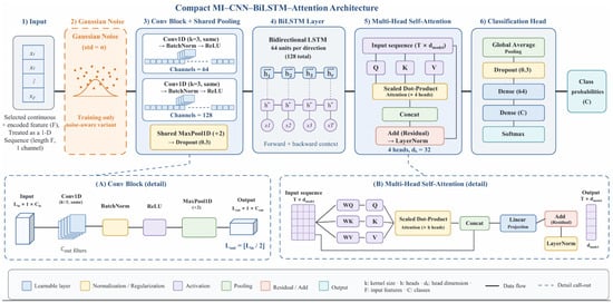
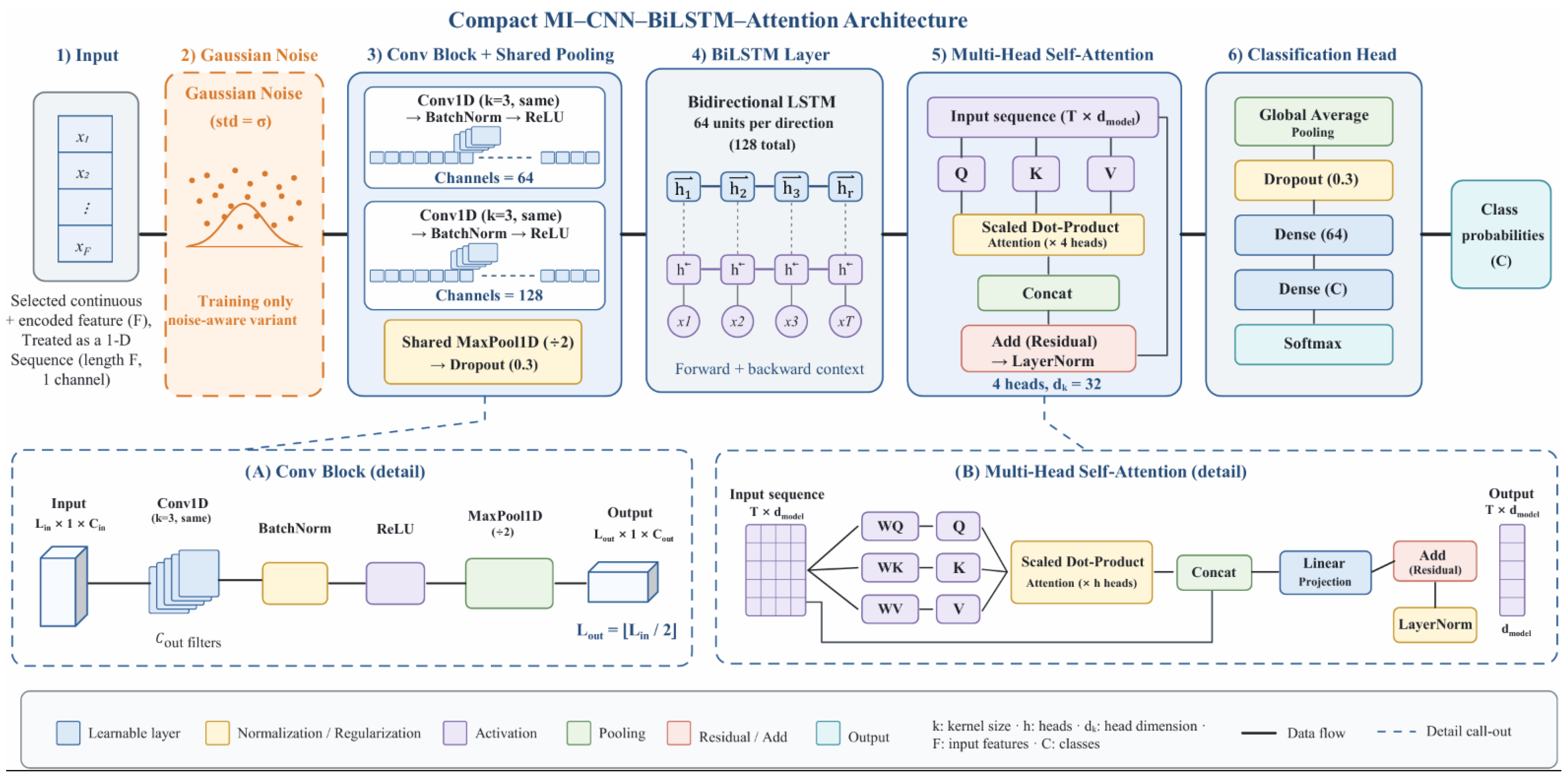
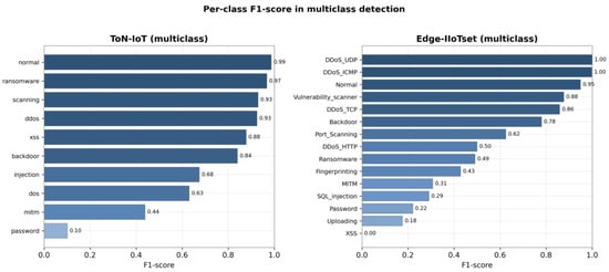
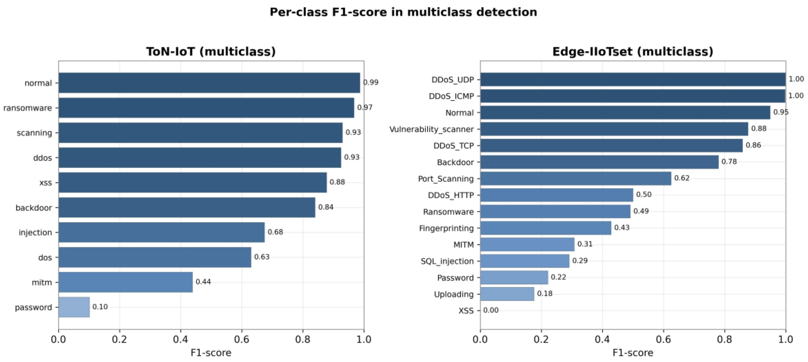
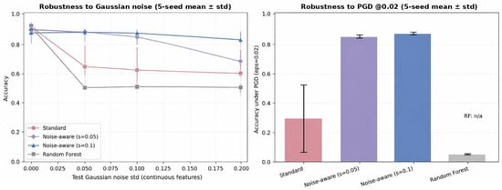
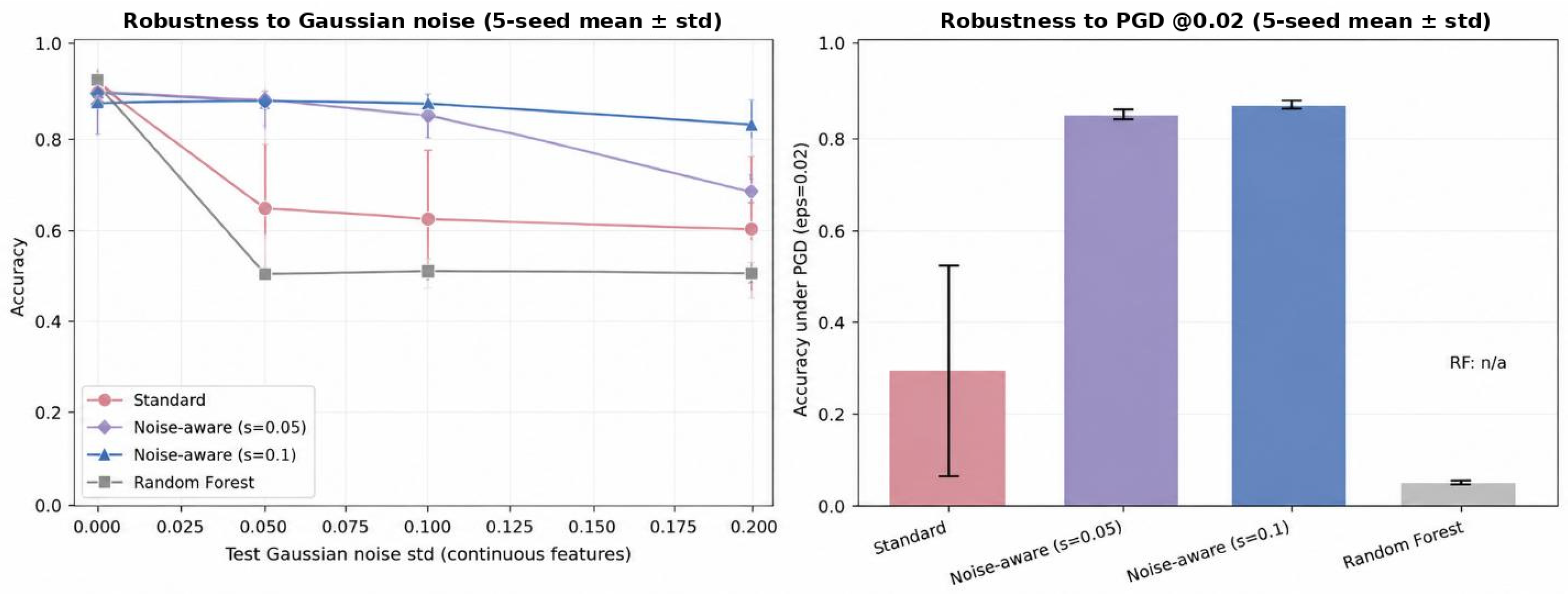
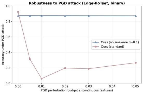
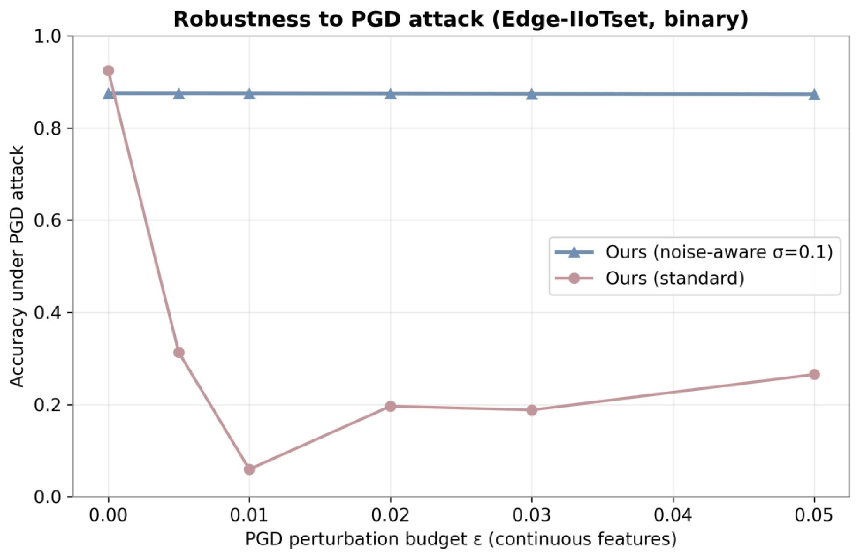
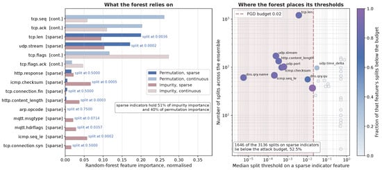
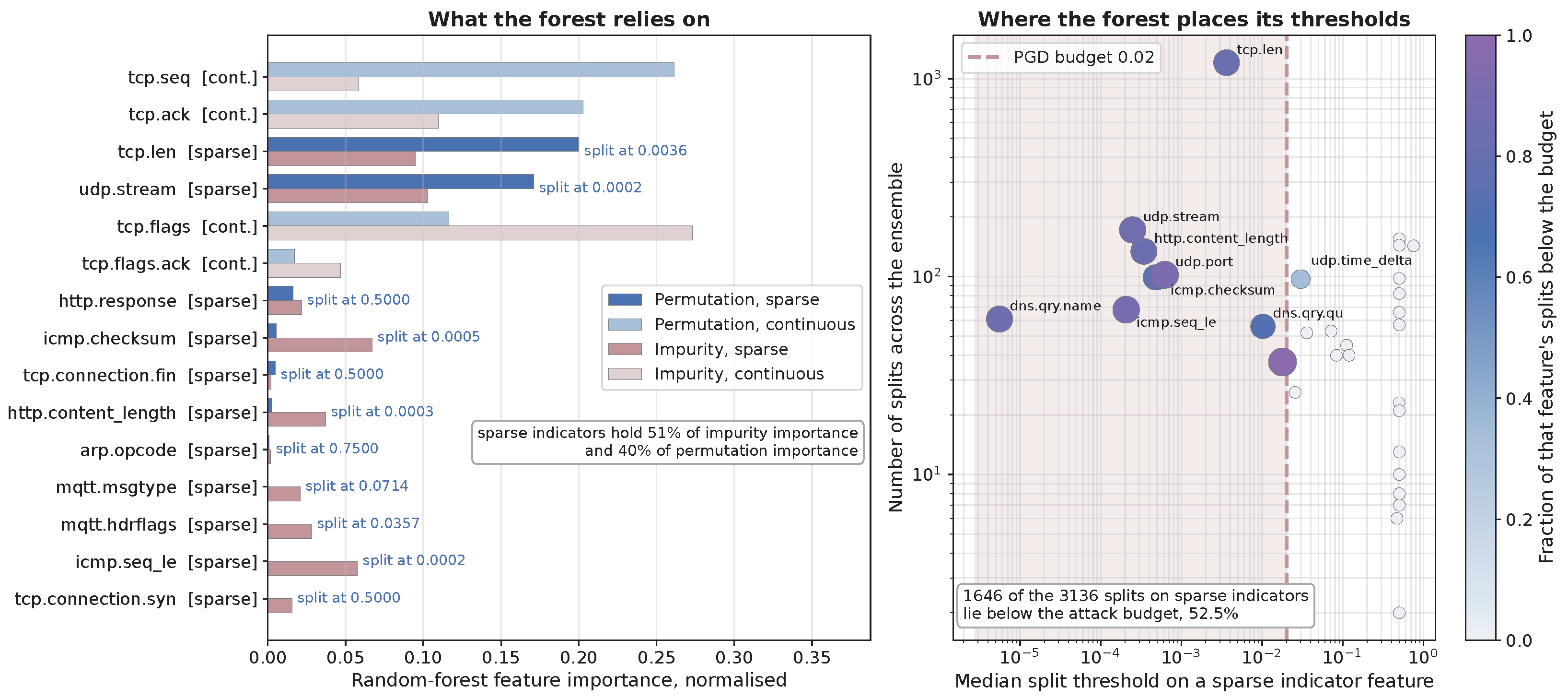
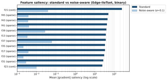
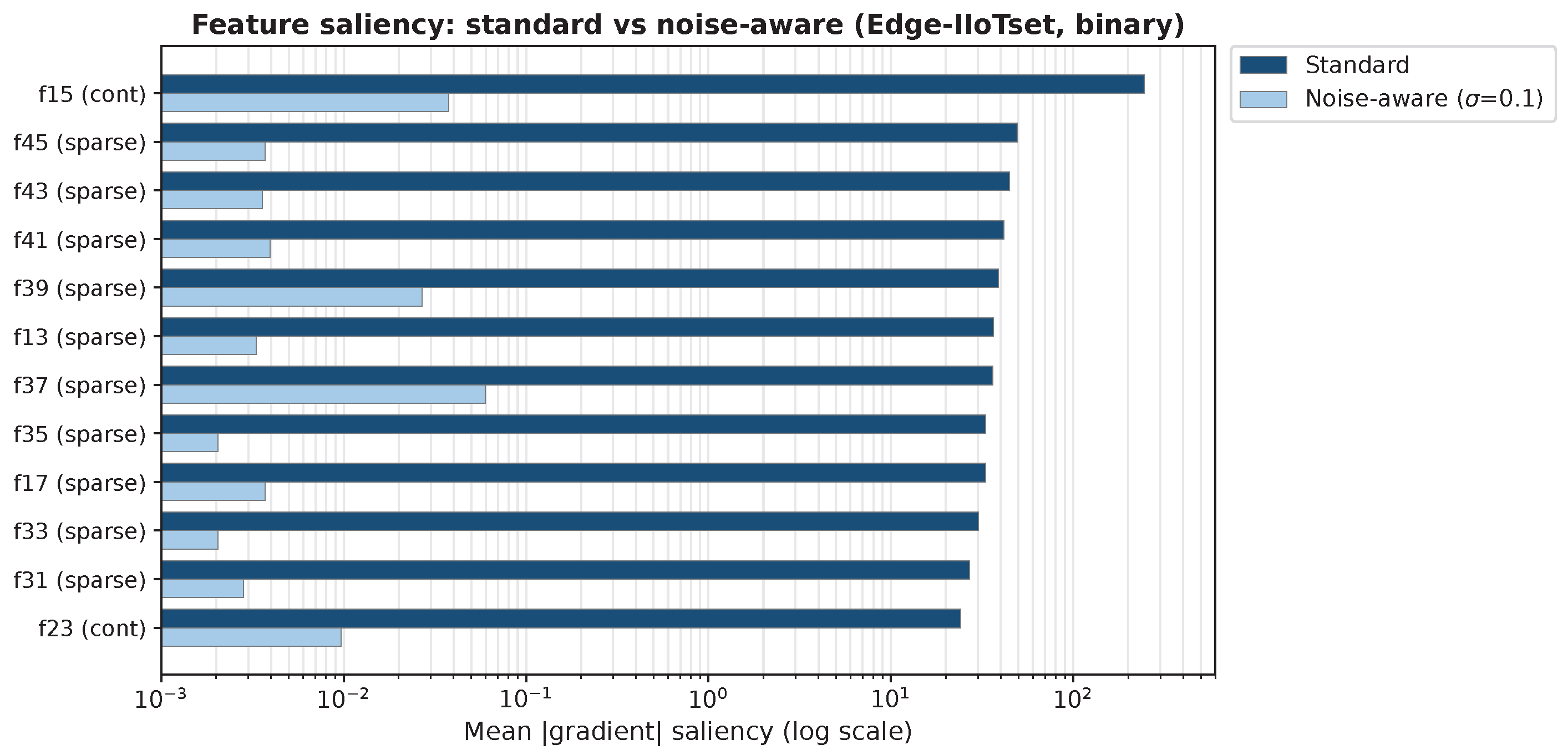
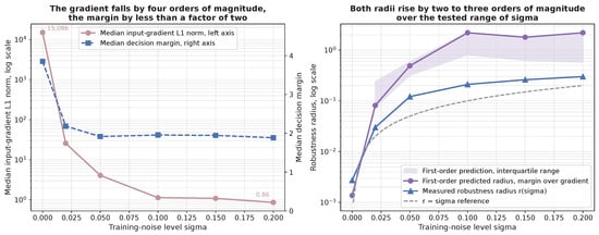
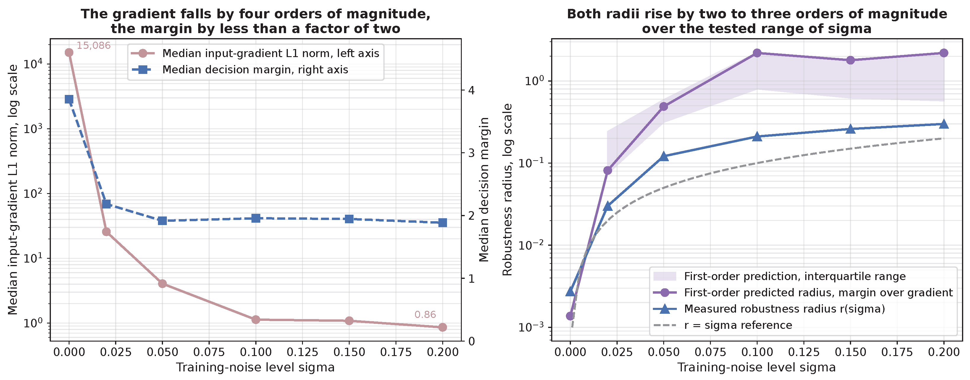
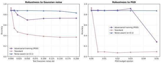
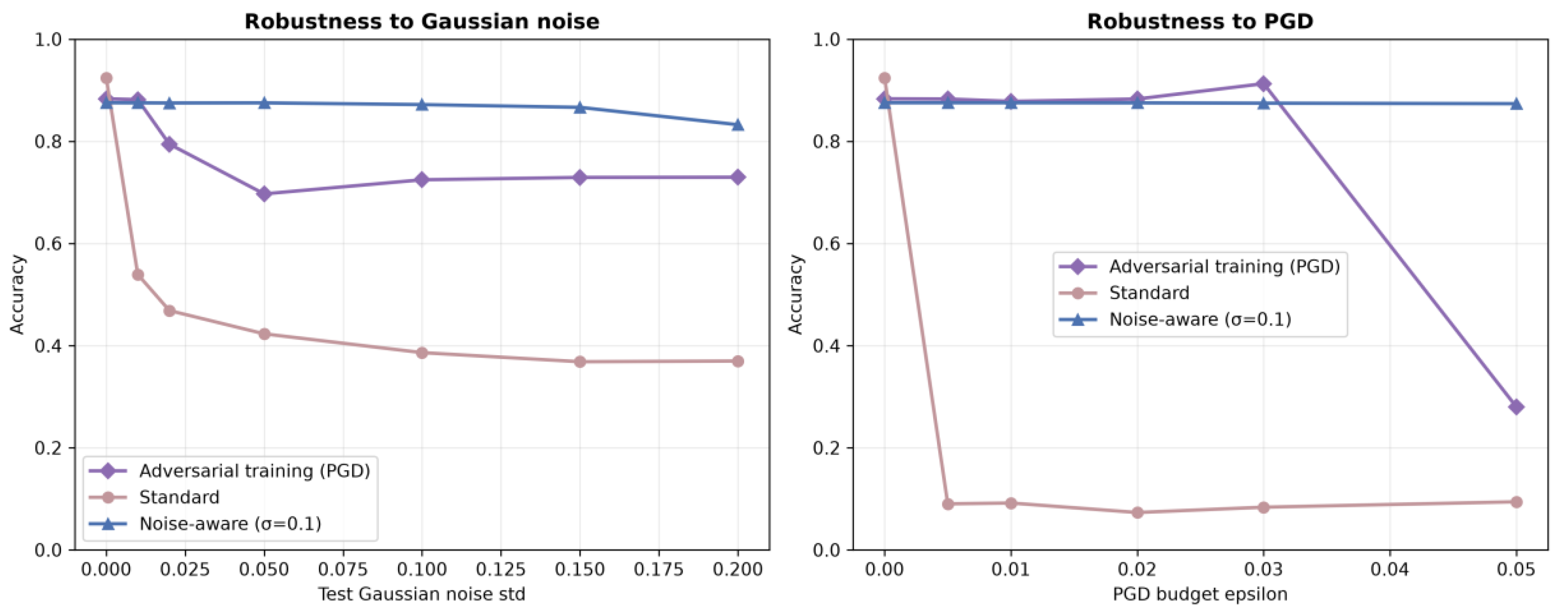
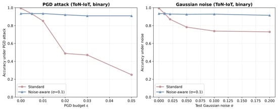
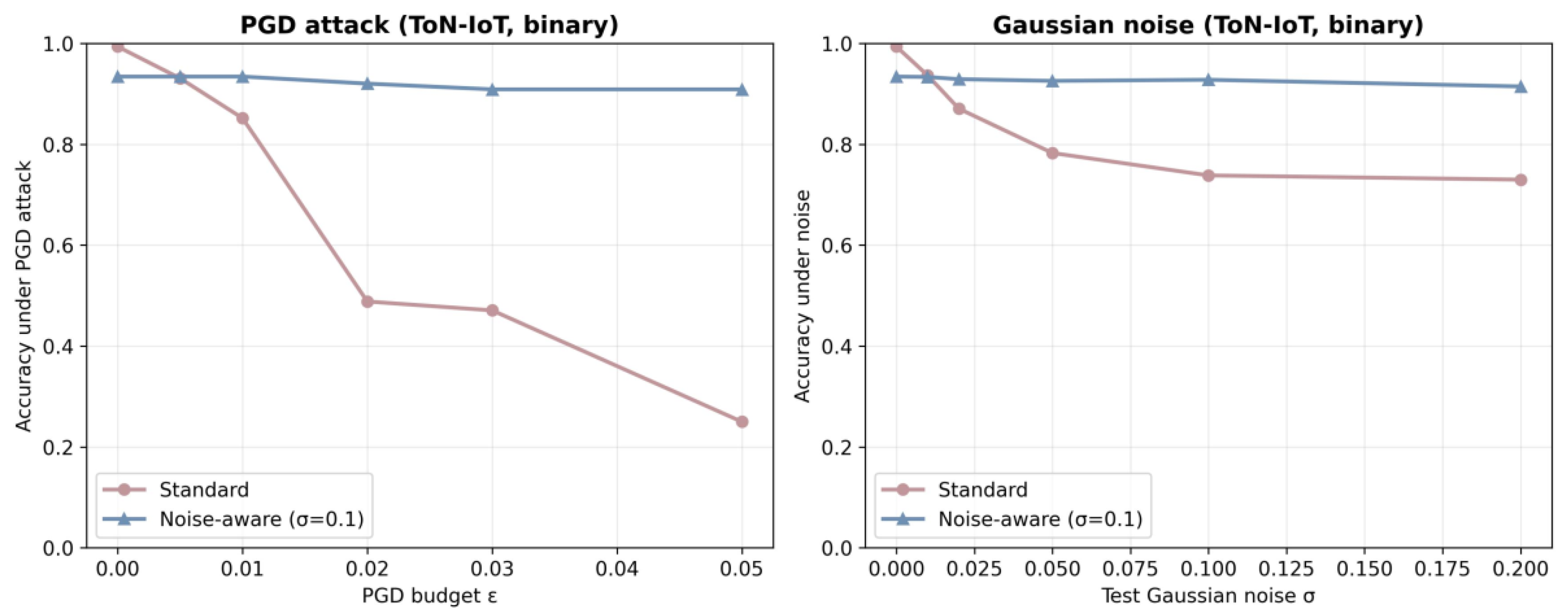
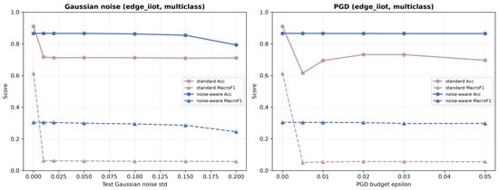
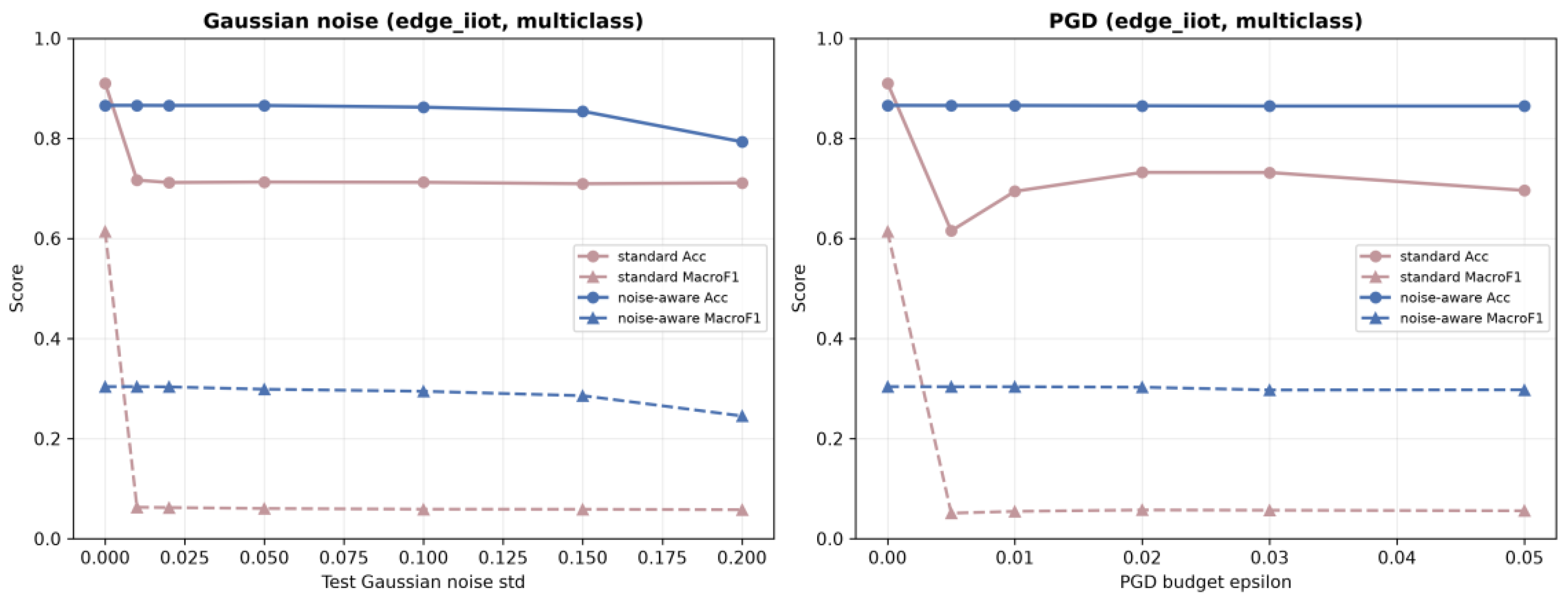
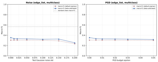
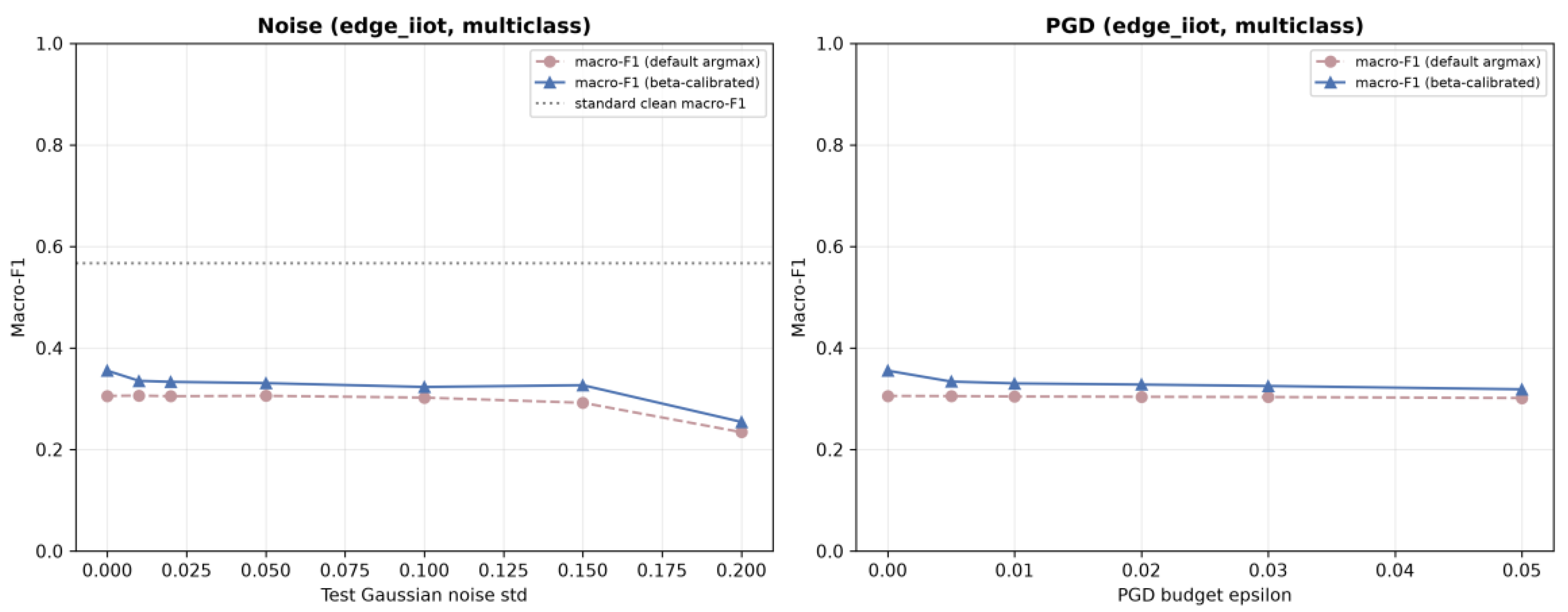
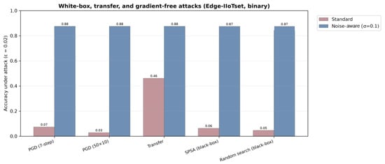
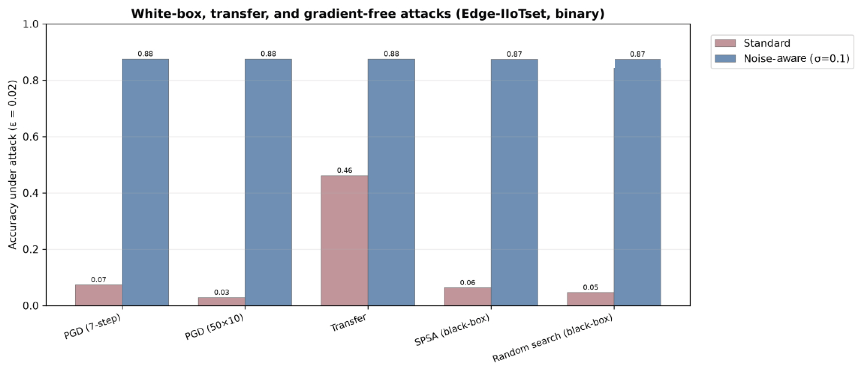
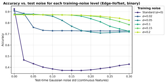
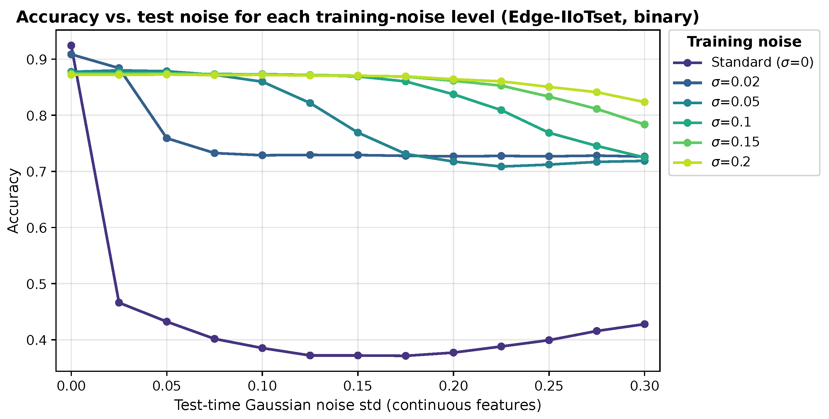
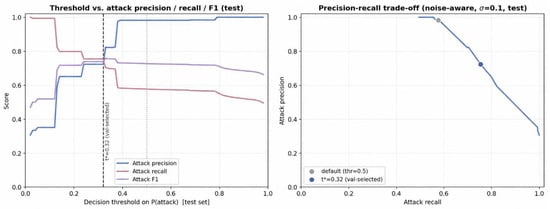
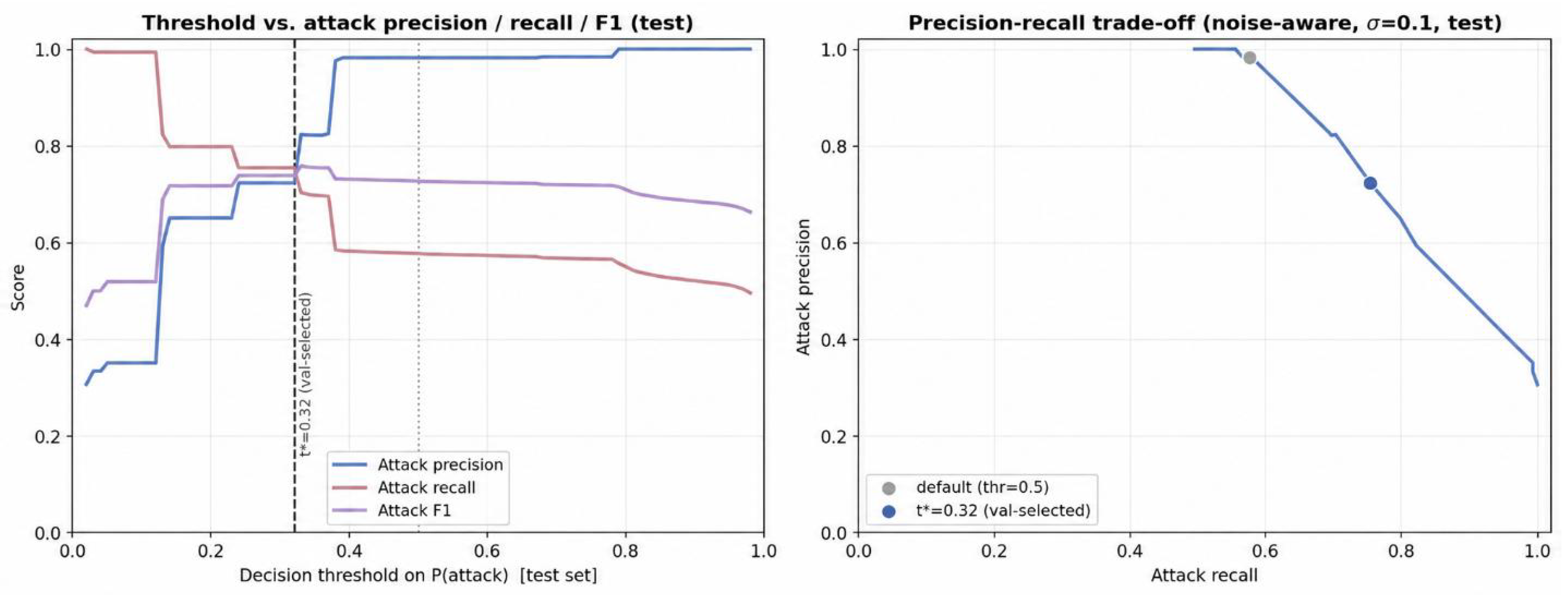
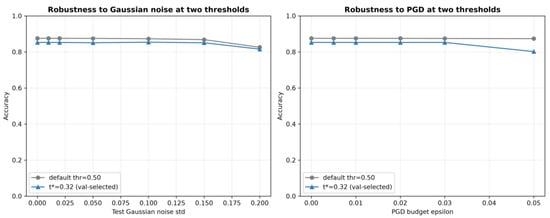
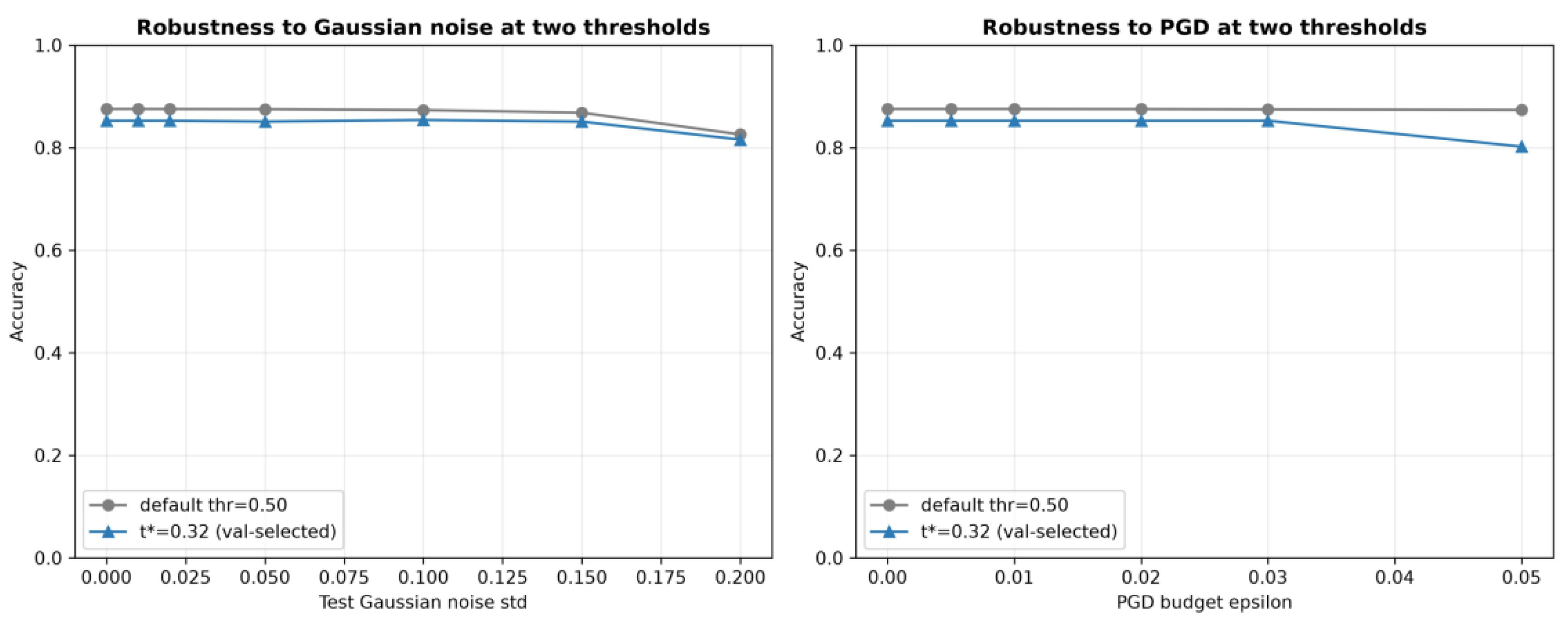

Disclaimer/Publisher’s Note: The statements, opinions and data contained in all publications are solely those of the individual author(s) and contributor(s) and not of MDPI and/or the editor(s). MDPI and/or the editor(s) disclaim responsibility for any injury to people or property resulting from any ideas, methods, instructions or products referred to in the content. |
© 2026 by the authors. Licensee MDPI, Basel, Switzerland. This article is an open access article distributed under the terms and conditions of the Creative Commons Attribution (CC BY) license.