


Featured Application
This study proposes a flexible framework for effectively bridging spatial coverage gaps in hyperspectral classification maps using multispectral imagery. This framework consists of a base classification component supporting diverse classifiers, alongside an optional cascade classification module and a lightweight reclassification module for spatial refinement. The results of evaluating mineral and general land use/land cover (LULC) classification demonstrate the practical utility and robustness of this framework.
Abstract
Hyperspectral (HS) sensors offer high spectral discrimination but generally limited spatial coverage, whereas multispectral (MS) sensors provide broad coverage with lower spectral detail. HS-MS complementary mapping aims to reduce coverage gaps in HS sensors by training classifiers within HS-MS overlap regions and applying them to surrounding MS-only areas. However, comprehensive comparisons across classifiers remain scarce in this complementary mapping setting. Furthermore, lightweight pixel-wise classifiers often produce spatially inconsistent predictions, whereas spatial–spectral deep learning models demand substantial computational resources. In this study, we propose a flexible HS-MS complementary mapping framework by systematically evaluating 13 classifiers across mineral and land-use/land-cover (LULC) mapping tasks and introducing class-adaptive uncertainty revocation (CAUR), a lightweight, classifier-independent post-processing module. Performance was evaluated via spatial holdout cross-validation within the HS-MS overlap area. When computational resources are sufficient, 3D convolutional neural networks (3D-CNN) achieve the highest accuracy. Conversely, lightweight models such as random forest (RF) and k-nearest neighbors (kNN) provide computationally efficient and robust baselines. Applying CAUR consistently improves spatial consistency and overall classification accuracy without model retraining, with the largest improvements observed for coarser-resolution HS reference data. These findings provide practical design guidelines for constructing efficient HS-MS complementary mapping pipelines tailored to application demands and sensor characteristics.
Keywords:
classification; machine learning; mineral mapping; land use and land cover; AVIRIS; HISUI; EMIT; ASTER 1. Introduction
Remote sensing is widely used for applications such as mineral exploration and land-use/land-cover (LULC) classification [1,2,3,4,5,6,7,8]. Multispectral (MS) sensors provide broad spatial coverage but have limited spectral resolution, making it difficult to distinguish spectrally similar materials [1,9,10]. Hyperspectral (HS) sensors overcome this limitation by capturing hundreds of contiguous spectral bands [11,12,13,14]. Although the number of operational HS sensors has increased in recent years [15,16,17,18,19,20,21,22,23,24,25,26], their narrower swath widths and lower observation frequency still limit spatial coverage [14]. For example, the Japanese spaceborne HS sensor HISUI (which completed its operational mission on the International Space Station in 2023) had a narrow 20 km swath width, and cloud cover further reduced the number of usable observations [18,19,20,21,22,23].
A practical way to exploit the complementary characteristics of HS and MS data is HS–MS map complementation. In this technique, classification models are trained in areas where HS and MS images overlap and are subsequently applied to surrounding regions covered only by MS imagery, thereby extending HS-derived classification maps over much larger areas. Early approaches relied on physical spectral matching between HS and MS data [26,27,28,29,30,31,32,33]. More recently, machine-learning-based approaches have become the primary alternative [34]. Ni et al. [34] proposed a support vector machine (SVM)-based framework for crop mapping, whereas Tsubomatsu and Tonooka [35] introduced a random forest (RF)-based cascade framework (hereinafter referred to as the TT method) for mineral mapping, drawing on hierarchical expert systems [36].
Alongside these direct HS-MS complementary mapping efforts, the broader field of multi-source remote sensing fusion has advanced substantially. State-space models such as MSFMamba [37] enable multi-scale feature fusion from heterogeneous sensors with linear computational complexity; multi-scale interactive fusion networks (MIFNet [38]) demonstrate effective cross-modal representation learning for HS and synthetic aperture radar (SAR) classification; and cross-scale self-supervised frameworks such as Cross-Scale MAE [39] provide scale-robust representations. However, general multi-source fusion methods typically assume concurrent multi-sensor coverage across the entire study area, whereas HS-MS complementary mapping is subject to specific constraints: training is strictly confined to overlapping regions, and the model must generalize across spatially disjoint MS areas. The first challenge therefore concerns the lack of comprehensive evaluations. Existing studies on HS-MS complementary mapping [26,27,28,29,30,31,32,33,34] have evaluated only isolated classifier types (typically RF or SVM) under varying conditions, leaving it unclear which classifiers are best suited to these constraints and how classifier properties interact with post-classification refinement.
A second challenge concerns the spatial consistency of the resulting classification maps. Because most existing methods assign labels to each pixel independently, prediction errors frequently appear as isolated misclassified pixels and fragmented class boundaries, commonly referred to as salt-and-pepper noise [40]. Spatial–spectral deep learning architectures such as 3D-CNNs and U-Nets can, in principle, reduce these artifacts by incorporating neighborhood information during training. In HS-MS complementary mapping, however, training samples are inherently confined to the relatively small overlap region between HS and MS observations. Under this constraint, patch-based architectures require more spatially distributed training data than is typically available and are therefore prone to overfitting [41]. A practical alternative is a lightweight post-classification refinement step that operates on the probability outputs of any existing pixel-wise classifier without modifying its training process.
For such a refinement to be effective, it must account for a structural characteristic of classification uncertainty in remote sensing data. Prediction uncertainty, commonly quantified using the Shannon entropy of the posterior class-probability distribution, varies systematically among classes rather than merely between correct and incorrect predictions. Classes with well-defined spectral signatures produce consistently low-entropy outputs, whereas classes affected by spectral overlap or mixed-pixel effects yield systematically high-entropy, ambiguous predictions [42,43,44]. Global filtering approaches, such as conventional majority filtering [45,46] or uniform entropy thresholds [47,48], make it difficult to balance these class-dependent differences. Majority filtering unconditionally overwrites isolated pixels, risking the loss of valid fine structures, while uniform entropy thresholds systematically discard information from spectrally ambiguous or rare classes. Class-specific adaptive thresholds are therefore essential to calibrate uncertainty evaluation to the intrinsic spectral separability of each class. This class-adaptive principle builds upon the design philosophy of the TT method [34] and extends it to general multi-class mapping tasks.
Motivated by these observations, we propose a flexible, classifier-independent HS-MS complementary mapping framework. Unlike the TT method [34], which relies on a fixed RF classifier, mineral-specific features, and a mandatory cascade structure, the proposed framework decouples base classification from spatial post-processing and treats the cascade as an optional module. As the post-classification component, we introduce class-adaptive uncertainty revocation (CAUR). Unlike existing post-processing approaches [42], CAUR integrates probability diffusion, class-specific uncertainty detection, and spatial-isolation evaluation. Specifically, it selectively revokes predictions that are both highly uncertain and spatially isolated, and subsequently reconstructs them using reliable neighborhood labels, improving spatial consistency without base classifier retraining.
The contributions of this study are threefold. First, we propose a flexible framework for HS–MS complementary mapping that generalizes the TT method across diverse classifiers and mapping tasks. Second, we present the first systematic benchmark of 13 machine-learning classifiers under identical spatial holdout conditions, providing empirical design guidelines across sensor types and application domains. Third, we introduce CAUR as a lightweight post-processing module and characterize the contribution of each internal mechanism through a comprehensive ablation analysis.
The remainder of this paper is organized as follows. Section 2 describes the study sites, datasets, baseline classifiers, the proposed CAUR framework, and the experimental design. Section 3 presents the experimental results. Section 4 discusses the findings in relation to sensor characteristics, classifier properties, and framework mechanisms. Finally, Section 5 concludes the study.
2. Materials and Methods
2.1. Study Sites and Data
2.1.1. Study Sites
Two study sites were used: the Cuprite mining district (Nevada, USA) and the Mito City surrounding area (Ibaraki, Japan), each covering approximately 150 km2. Cuprite is characterized by extensive hydrothermal alteration and has been widely used for hyperspectral mineral mapping studies [9,49,50]. In contrast, the Mito site contains a mixture of urban areas, agricultural land, forests, and water bodies, providing diverse land-cover conditions for LULC classification [51]. For both sites, the analysis area was defined as the region jointly covered by all hyper- and multispectral datasets used in this study. Figure 1 shows the study locations.
Figure 1.
Study sites used in this research. For each site, the left panel shows the regional overview and the right panel shows a close-up view of the analysis area displayed as an ASTER false-color composite (R: band 2, G: (band 1 × 3 + band 3)/4, B: band 1), with latitude/longitude graticules and a north arrow. (a) Cuprite mining district, Nevada, USA. (b) Mito City (surrounding area), Ibaraki Prefecture, Japan.
2.1.2. Sensors
Three HS sensors (AVIRIS, HISUI, and EMIT) and one MS sensor (ASTER) were evaluated. Their main specifications are summarized in Table 1.
Table 1.
Basic specifications of AVIRIS [15,52], HISUI [21], EMIT [23], and ASTER [7,8].
The three HS sensors employed in this study (AVIRIS, HISUI, and EMIT) all cover the visible-to-shortwave infrared (VSWIR) spectral range. In contrast, the MS sensor ASTER acquires multispectral data across the visible and near-infrared (VNIR), shortwave infrared (SWIR), and thermal infrared (TIR) regions. AVIRIS [15,52] and EMIT [23] were developed by the National Aeronautics and Space Administration (NASA), United States whereas HISUI [21] and ASTER [7,8] were developed by Japan’s Ministry of Economy, Trade and Industry (METI). These sensors differ in spectral and spatial resolution, providing diverse data characteristics suitable for evaluating HS-MS complementary mapping across varying sensor configurations.
2.1.3. Datasets and Preprocessing
The datasets used in this study are summarized in Table 2, which provides detailed acquisition dates, processing levels, and product IDs.
Table 2.
Detailed information for the datasets used in this study.
For the Cuprite site, AVIRIS, HISUI, EMIT, and ASTER datasets were used. The ASTER scene was acquired in August 2006, approximately one month before the AVIRIS observation, and retains all SWIR bands. For the HISUI-ASTER and EMIT-ASTER combinations at Cuprite, the temporal differences span 15 and 18 years, respectively. Acquisition months were September for AVIRIS, April for HISUI, June for EMIT, and August for ASTER. Although Cuprite is an arid, sparsely vegetated environment where hydrothermally altered mineral distributions remain highly stable over decadal timescales [9,49,50,53], transient vegetation may exhibit minor seasonal variation. However, its influence on rock-dominated mineral signatures is expected to be minimal. Because the ASTER SWIR subsystem ceased operation in 2008, only the ASTER VNIR and TIR bands were utilized for the HISUI-ASTER and EMIT-ASTER pairings [7,8].
For the Mito site, HISUI and EMIT were paired with ASTER. All three sensor acquisitions were timed to mid-winter (HISUI: January 2022, EMIT: January 2025, ASTER: December 2021) to minimize seasonal differences in vegetation phenology and solar illumination. The HISUI-ASTER pair has a temporal gap of approximately one month, while the EMIT-ASTER pair spans approximately three years. Regarding the ASTER band configuration, SWIR bands were excluded because a previous study [51] demonstrated that cross-temporal reflectance drift in the SWIR region degrades classification accuracy at the Mito site, and relatively few LULC classes at this site rely strongly on SWIR spectral features. Therefore, only contemporary ASTER VNIR and TIR data were used for all Mito experiments. The longer temporal interval of the EMIT-ASTER pair may introduce a limited risk of localized land-cover change, such as construction or agricultural conversion, which is recognized as a study limitation (Section 4.4).
Sensor spatial resolution varies across the evaluated platforms. The coarser resolution of EMIT (60 m) compared to AVIRIS (4–20 m) and HISUI (20–31 m) inherently increases the fraction of spectrally mixed pixels along class boundaries and for spatial features smaller than the 60 m ground resolution cell, thereby reducing spectral separability. The implications of this resolution difference for classification variance are discussed in Section 4.1.
All datasets were geometrically corrected and co-registered. Pre-geometrically corrected products (ASTER L1T and HISUI L1G) were used, and visual landmark inspection confirmed residual misregistration within one pixel. Atmospheric correction for ASTER L1T radiance data was conducted using the fast line-of-sight atmospheric analysis of spectral hypercubes (FLAASH) module in ENVI 6.3 (NV5 Geospatial, Inc., Superior, CO, USA) [54] to obtain surface reflectance. In contrast, EMIT L2A data were acquired directly as atmospherically corrected surface reflectance. Spatial atmospheric conditions were assumed to be uniform across each scene [34].
For all datasets, hyperspectral bands overlapping major atmospheric water vapor absorption regions (~1.4 um and ~1.9 um) were removed prior to analysis. Cloud and shadow areas were identified and masked using visual screening and EMIT L2A quality control flags.
For model training and evaluation, HS and MS data were aligned to a common spatial grid using nearest-neighbor interpolation. AVIRIS–ASTER and HISUI–ASTER pairs were resampled to the 15 m ASTER VNIR grid, whereas EMIT–ASTER pairs were resampled to the 60 m EMIT grid.
2.1.4. Reference Data Preparation
Reference maps were derived from HS imagery within the HS–MS overlap regions. These maps served both as training labels for MS-based classification and as ground reference for evaluating the extended classification maps.
Reference maps were produced using either the Hourglass workflow implemented in ENVI [55,56,57,58] or the Tetracorder expert system of the United States Geological Survey (USGS) [36,58,59]. Hourglass was applied to both the Cuprite and Mito datasets, whereas Tetracorder was applied only to the Cuprite datasets because it is specifically designed for mineral identification. The resulting HS-derived reference datasets are summarized in Table 3. Hereafter, each reference dataset is identified by the combination of the HS sensor and reference-map generation method (e.g., AVIRIS–Hourglass, HISUI–Hourglass, and EMIT–Tetracorder).
Table 3.
Summary of the HS-derived reference datasets used in this study.
It should be noted that the Hourglass and Tetracorder outputs represent HS-sensor-derived reference maps rather than independently validated ground truth obtained through systematic field surveys. The reliability of the Cuprite mineral reference maps is substantiated by their quantitative spectral correlation (spectral fit score > 0.85–0.90 against USGS library endmembers) and spatial consistency with published USGS geological alteration maps [9,49,50,53]. Specifically, major mineral zones (including alunite, kaolinite, buddingtonite, and calcite) are coherently delineated across the Hourglass and Tetracorder outputs and are geographically consistent with the USGS reference. The Mito LULC reference maps were validated across representative land-cover zones using high-resolution orthophotography and sampling verification [60], confirming high labeling fidelity for major classes. Nonetheless, the uncertainties inherent in the algorithms used to generate the reference maps cannot be fully eliminated for either site, and their potential influence on baseline accuracy evaluations is recognized as an inherent study limitation (Section 4.4).
2.2. Classification Methods
2.2.1. Baseline Classifiers
A total of 13 representative machine-learning classifiers were evaluated to investigate the influence of classifiers themselves on HS–MS map complementation. The evaluated methods included Gaussian Naive Bayes (GNB) [61], k-nearest neighbors (kNN) [62], logistic regression (LR) [63], multi-layer perceptron (MLP) [64], linear support vector classification (SVC) optimized via stochastic gradient descent [65], 1D convolutional neural network (1D-CNN) [66], TabNet [67], 3D convolutional neural network (3D-CNN) [68], and U-Net [69]. To examine tree-based methods, RF [70] and three related variants were additionally evaluated: one-versus-rest RF (OvR-RF) [71], edge-preserving filter RF (EPF-RF) [72], and XGBoost [73]. The 13 classifiers selected cover a broad range of machine-learning approaches commonly used for remote sensing image classification.
All classifiers were trained on the HS-derived reference maps described in Section 2.1.4 and subsequently applied to MS data to generate the complemented classification maps. Hyperparameter settings and evaluation procedures are described in Section 2.3.
2.2.2. Proposed CAUR Framework
CAUR is a post-processing framework applied after any supervised classifier has generated class probabilities and predicted labels, designed to improve pixel-wise classification maps by correcting unreliable predictions. Because CAUR operates only on these outputs, it can be combined with a wide variety of classifiers without modifying their internal learning algorithms. Unlike spatial–spectral classifiers that incorporate neighborhood information during training, CAUR refines classification results as a post-processing step. Specifically, it selectively revises pixels that are both highly uncertain and spatially isolated while preserving reliable predictions. This strategy reduces salt-and-pepper noise without unnecessarily smoothing class boundaries.
The CAUR procedure consists of four stages: (1) class-adaptive entropy-threshold optimization, (2) uncertainty detection, (3) uncertainty-guided label revocation and neighborhood agreement evaluation, and (4) iterative neighborhood reconstruction. Hyperparameters for both the base classifiers and CAUR were optimized using Optuna [74], which employs Bayesian optimization for efficient hyperparameter search, thereby ensuring objective and data-driven parameter selection. A schematic overview of the complete CAUR workflow is presented in Figure 2.
Figure 2.
Flowchart of the CAUR framework, illustrating the parallel pathways for out-of-bag (OOB)/cross-fitted ensemble classifiers and boundary-pixel proxy estimation for non-OOB models, followed by uncertainty detection, neighborhood agreement evaluation, and iterative spatial reconstruction.
- (1)
- Probability Diffusion and Class-Adaptive Entropy-Threshold Optimization
Shannon entropy is widely applied to quantify prediction uncertainty from posterior probability distributions because it measures the ambiguity among competing class assignments [44,75,76]. Before entropy calculation, a probability diffusion step incorporates the local spatial context into the raw class probabilities. Specifically, the probability map for each class is smoothed by blending the original probability with the average probability across the entire 3 × 3 local window in a 7:3 ratio.
The 7:3 blend ratio and 3 × 3 window size were determined through a preliminary grid search on the tuning area (Section 2.3.1), in which blend ratios of {5:5, 6:4, 7:3, 8:2} and window sizes of {3 × 3, 5 × 5} were evaluated. The 7:3 ratio with a 3 × 3 window achieved the highest Macro-F1 by balancing local noise suppression and fine boundary preservation. These parameters were fixed throughout all subsequent experiments and were excluded from the hyperparameter optimization performed by Optuna.
The Shannon entropy for pixel is calculated as defined in Equation (1):
where denotes the entropy of pixel , is the number of classes, is the predicted posterior probability that pixel belongs to class , and is a small constant introduced to prevent numerical instability when evaluating the logarithm of zero.
For classifiers supporting out-of-bag (OOB) estimation (specifically RF, OvR-RF, and EPF-RF), entropy thresholds are optimized independently for each class using OOB predictions [77,78]. Candidate thresholds are sampled from the class-specific entropy distribution on the training data. For each candidate’s threshold, training pixels exceeding the threshold are temporarily marked as Unknown and excluded from the Macro-F1 calculation. The threshold yielding the highest Macro-F1 score under this procedure is selected as the optimal entropy threshold for class . Note that the iterative neighborhood reconstruction step is not performed during threshold optimization; it runs only in the post-processing phase. Threshold selection therefore reflects the direct effect of uncertainty filtering alone before spatial reconstruction is applied.
For classifiers lacking OOB estimation (specifically XGBoost, GNB, kNN, LR, SVC, MLP, 1D-CNN, TabNet, 3D-CNN, and U-Net), class-specific entropy thresholds are estimated using training-set predictions restricted to boundary pixels. Boundary pixels are defined as training pixels that have at least four spatial neighbors belonging to different classes in the reference map. Because boundary pixels exhibit greater spectral mixing and higher error rates, class-specific F1-scores computed on these pixels serve as a proxy for boundary reliability. The revocation rate for class c is set to , ensuring that classes with lower boundary reliability receive higher revocation proportions. Within each class, pixels are revoked in descending order of entropy until the target revocation rate is reached. For XGBoost specifically, cross-fitted probability estimates obtained through k-fold cross-validation on the training data are used in place of boundary-pixel proxies, under the same Macro-F1 maximization procedure as for OOB-capable classifiers.
The hyperparameters optimized via Optuna are the per-class entropy thresholds for OOB and cross-fitted classifiers, the maximum number of reconstruction iterations, and the minimum neighborhood agreement threshold .
- (2)
- Uncertainty Detection
A pixel is regarded as uncertain when its entropy exceeds the threshold assigned to its predicted class. This uncertainty state is defined as expressed in Equation (2):
where denotes the predicted class label of pixel .
- (3)
- Neighborhood Agreement Evaluation and Label Revocation
Pixel-wise classification frequently produces isolated misclassified pixels (salt-and-pepper noise) in remote sensing imagery [40]. Neighborhood agreement was therefore used together with prediction uncertainty to identify unreliable pixels. For pixel , the neighborhood agreement is calculated as expressed in Equation (3):
where denotes the neighborhood surrounding pixel (excluding the center pixel itself), is the number of neighboring pixels, and is the indicator function, taking the value 1 when and 0 otherwise.
Pixels are marked for revision only when both high uncertainty and low neighborhood agreement are observed. This revision condition is formulated as expressed in Equation (4):
where is the minimum neighborhood-agreement threshold.
The uncertainty indicator is computed once from the original class-probability distribution and remains fixed throughout the iterative reconstruction. In contrast, the neighborhood agreement is updated at each iteration according to the current label configuration. Pixels satisfying Equation (4) are temporarily assigned an “Unknown” label, as expressed in Equation (5):
- (4)
- Iterative Neighborhood Reconstruction
Pixels labeled as “Unknown” are iteratively reconstructed using the most frequent class among neighboring valid pixels. The updated label is calculated as expressed in Equation (6):
This reconstruction process is repeated until either all “Unknown” pixels are assigned a class label or the predefined maximum number of iterations (a hyperparameter optimized via Optuna) is reached.
In rare cases where a pixel remains unresolved after the reconstruction process, the original classifier prediction is restored. This final fallback assignment is calculated as expressed in Equation (7):
where denotes the original class-probability distribution before refinement.
2.2.3. Configurations for Ablation Study
To evaluate both the overall effectiveness of the proposed framework and the contribution of each processing stage, eight comparison configurations were prepared. The complete framework (CAUR_FULL) served as the reference configuration.
- (1)
- Baseline and Existing Methods
These configurations compare the proposed framework with the original classifier and representative post-processing methods:
- RAW_BASELINE: RF classification without post-processing.
- MAJORITY_FILTER: A conventional 3 × 3 majority filter applied directly to the hard-label classification map.
- CASCADE_ONLY: A simplified version of the original TT framework in which the mineral-specific Band Math feature expansion was removed while retaining the cascade classification structure. This configuration was evaluated only for the Cuprite datasets because the cascade framework is specific to mineral mapping.
- TT_ORIGINAL: The original TT framework proposed in our previous study [34]. This comparison was limited to the Cuprite datasets because TT_ORIGINAL relies on mineral-specific Band Math features that are unavailable for LULC classification.
- (2)
- Ablation Configuration
Each ablation configuration removes one processing stage while keeping all remaining components unchanged:
- NO_RECONSTRUCTION: Uncertain pixels are revoked as in the complete framework, but neighborhood reconstruction is skipped. Pixels remaining as “Unknown” are restored to their original classifier labels at the end of the procedure.
- NO_DIFFUSION: Probability diffusion is disabled, and entropy is computed directly from the original class-probability distribution.
- NO_SPATIAL: Spatial-consistency evaluation is disabled. Pixels are revoked solely according to their entropy without considering neighborhood agreement.
- GLOBAL_THRESHOLD: Class-adaptive entropy thresholds are replaced with a single global threshold optimized across all classes.
All configurations were evaluated using RF as the base classifier, with a supplementary experiment using kNN, as reported in Appendix D. Hyperparameters were fixed to the values determined during the optimization procedure described in Section 2.3.2.
2.3. Evaluation Setup and Metrics
2.3.1. Evaluation Design
Hyperparameter optimization was conducted on a geographically independent tuning area of approximately 50 km2 located north of the Cuprite evaluation site. This area was evaluated using the AVIRIS–Hourglass reference map due to its high spatial resolution and abundant labeled samples. The optimized hyperparameters were subsequently applied without modification to all evaluation datasets, including the Mito site. Applying the same hyperparameters to all evaluation datasets—including the geographically and spectrally distinct Mito site—allows us to assess whether the framework generalizes robustly across different environments without tuning to site-specific conditions. Note that the evaluation regions at Cuprite and Mito were excluded from hyperparameter tuning.
To evaluate model generalizability across geographically separated sub-regions, classification performance was assessed via spatial holdout cross-validation within the HS–MS overlap area. Training samples were extracted using stratified sampling [2] to ensure that minority classes were adequately represented in each fold. Direct empirical validation in regions beyond the HS coverage requires ground reference data for those regions; because such data were unavailable in this study, validation outside the overlap regions was not conducted. Nonetheless, multispectral feature statistics (mean and variance across ASTER bands) showed a relative difference of less than 5% between the overlap regions and the surrounding MS-only areas. While this indicates a high degree of spectral consistency across the scene, this constraint should be considered when interpreting the evaluation results.
The final classification performance was evaluated using spatial holdout cross-validation to account for spatial autocorrelation. In each fold, two rectangular test regions (each approximately 1 km × 1 km) were designated such that all target classes were represented within the combined test area. A two-pixel buffer surrounding each test region was excluded from both training and testing sets to prevent spatial information leakage. Four independent spatial holdout splits were evaluated for each dataset, and performance is reported as the mean across folds.
Dataset-specific adjustments were applied to ensure fair comparisons across sensors. For Cuprite mineral mapping, classes containing fewer than 1000 labeled pixels within any test region were excluded from evaluation because certain classes identifiable in AVIRIS and HISUI reference maps could not be reliably extracted from EMIT reference maps owing to its coarser spatial resolution and lower signal-to-noise ratio. This exclusion ensured that all Cuprite sensor combinations were evaluated on the same subset of mineral categories. For Mito LULC mapping, spectrally ambiguous categories affected by mixed-pixel transitions were merged into semantically coherent parent classes prior to training and evaluation.
2.3.2. Implementation and Hyperparameter Optimization
All classifiers were implemented in Python using scikit-learn (v1.3.0) [79], XGBoost (v1.7.0) [73], and PyTorch (v1.10.0) (for 1D-CNN, TabNet, 3D-CNN, and U-Net).
Input features were standardized to zero mean and unit variance using StandardScaler from scikit-learn. Scaling parameters were fitted exclusively on the training folds and applied to the corresponding test splits without leakage. To mitigate class imbalance during training, ‘class_weight = ‘balanced’’ was applied to all scikit-learn classifiers [79]. For XGBoost, the ‘scale_pos_weight’ parameter was adjusted accordingly [73]. For PyTorch-based neural networks (1D-CNN, TabNet, 3D-CNN, and U-Net), inverse class-frequency weights were incorporated directly into the cross-entropy loss function [80].
Hyperparameters for baseline classifiers and the CAUR module were determined using Bayesian optimization in Optuna [74], with 20 trials allocated per model. Pilot experiments confirmed that 20 trials were sufficient for the Macro-F1 objective to achieve convergence. Detailed network architectures, implementation libraries, and Optuna hyperparameter search spaces for all 13 baseline classifiers and the CAUR module are summarized in Table A1 (Appendix A).
Computational efficiency was evaluated by recording model fitting time and inference prediction time separately. For CAUR, the recorded inference time encompasses probability diffusion, entropy computation, adaptive thresholding, spatial-isolation filtering, iterative reconstruction, and fallback recovery. All experiments were executed on a workstation equipped with an Intel Core i9-9900K CPU, 32 GB RAM, and an NVIDIA GeForce RTX 3080 GPU.
2.3.3. Evaluation Metrics
Classification performance was evaluated using macro-averaged F1-score (Macro-F1), overall accuracy (OA), and the Matthews correlation coefficient (MCC). Macro-F1 assigns equal weight to each class regardless of pixel frequency, making it appropriate for the class-imbalanced datasets common in remote sensing. Following the exclusion of classes absent from a given test fold, Macro-F1 was computed as the unweighted mean of per-class F1-scores; macro-averaged precision and recall were computed analogously. OA reports the proportion of correctly classified pixels, and MCC provides a balanced summary that accounts for all elements of the confusion matrix and is robust under class imbalance. Per-class F1-scores were additionally reported for detailed examination of class-level behavior. Cohen’s Kappa coefficient was included as a supplementary metric to facilitate comparison with previous studies. All performance values are presented as the mean ± standard deviation across the spatial cross-validation folds.
For the ablation study, RF was selected as the representative baseline classifier due to its consistent stability across mapping tasks. All ablation variants described in Section 2.2.3 were evaluated under identical spatial holdout splits and fixed hyperparameters. Performance differences were calculated as the score of CAUR_FULL minus that of the comparison configuration. Statistical significance was evaluated using the Wilcoxon signed-rank test [81], with each dataset-fold combination treated as a sampling unit. Because spatial folds originating from the same scene possess residual spatial correlations and pairwise comparisons were conducted without family-wise error rate corrections [81], these statistical tests are interpreted as indicative of performance trends rather than strict probabilistic bounds.
3. Results
3.1. Comprehensive Evaluation of Classifiers for HS–MS Complementary Mapping
3.1.1. Cuprite, Mineral Classification Mapping
The classification results for the five Cuprite reference datasets are summarized in Figure 3 (see Table 3 for the definitions of the datasets). Representative mineral-classification maps for the HISUI–Hourglass dataset are shown in Figure 4.
Figure 3.
Classification performance of baseline classifiers and their CAUR-refined counterparts across the five Cuprite reference datasets. Cell values indicate the mean ± standard deviation across spatial holdout folds. Both blocks use a red–blue color scale (red: higher/improvement, blue: lower/decrease) with different reference points: (a) Left block shows baseline performance relative to the RF baseline. (b) Right block shows performance changes after CAUR application relative to each corresponding baseline. The color scale for (b) is the same across all datasets.
Figure 4.
Representative mineral-classification maps generated from the HISUI–Hourglass reference dataset. Results for RF, kNN, and 3D-CNN are shown for both baseline and CAUR-refined classifications alongside the HS-derived reference map. White rectangles labeled “A” and “B” indicate the two spatial-holdout test regions used for evaluation (A: northern sub-region, B: southern sub-region). The bottom row displays magnified views of these two test regions, arranged from left to right (regions A and B, respectively).
The baseline classification performance varied widely among the classifiers. GNB and 1D-CNN consistently produced the lowest OA, Kappa, and MCC. In contrast, 3D-CNN and U-Net generally achieved the highest accuracies. Specifically, U-Net performed best on the AVIRIS–Hourglass and EMIT–Tetracorder datasets.
Other classifiers, including tree-based methods (XGBoost, EPF-RF, OvR-RF), kNN, TabNet, SVC, LR, and MLP, performed stably and competitively. For the AVIRIS–Tetracorder and EMIT–Hourglass datasets, these classifiers closely approached the accuracies of 3D-CNN and U-Net. Among the tree-based classifiers, the highest-performing method varied by dataset.
Across all methods, the AVIRIS–Tetracorder dataset yielded the lowest scores in OA, Macro-F1, Kappa, and MCC. The classification stability also varied by sensor type. Standard deviations were generally larger for the EMIT-derived datasets than for the AVIRIS and HISUI datasets. As discussed in Section 4, this larger variance is thought to be due to the coarser spatial resolution of EMIT (60 m), which reduced the number of available pixels within each 1 km × 1 km test region.
Applying CAUR generally improved OA, Kappa, and MCC across most classifiers, whereas improvements in Macro-F1 were more variable. CAUR produced the largest OA gains for RF, kNN, LR, and EPF-RF on the EMIT–Hourglass and AVIRIS–Tetracorder datasets. On the EMIT–Hourglass dataset, CAUR improved the accuracy for all classifiers. On the EMIT–Tetracorder dataset, accuracy improved for all classifiers except U-Net and LR. kNN showed performance gains from CAUR on all datasets except AVIRIS–Tetracorder.
Visual inspection of the classification maps (Figure 4) supports these results. The baseline maps from pixel-based classifiers such as RF and kNN showed severe salt-and-pepper noise in the test regions. CAUR effectively reduced this noise, producing continuous patches; 3D-CNN baseline maps exhibited substantially less noise, but CAUR still provided additional spatial smoothing. Occasionally, CAUR also smoothed regions where the HS-derived reference map itself contained fragmented label boundaries.
To examine class-level behavior, the per-class F1-scores for the Cuprite HISUI–Hourglass reference dataset across representative models (RF, kNN, and 3D-CNN, alongside their CAUR counterparts) are detailed in Table A2 (Appendix B). As indicated in Table A2, highly separable minerals such as alunite and nontronite consistently maintain high F1-scores across all classifiers, whereas rare minerals such as buddingtonite exhibit low scores owing to limited pixel counts.
3.1.2. Mito, Land Use and Land Cover Classification Mapping
The LULC classification performance was evaluated using the HISUI–Hourglass and EMIT–Hourglass datasets for Mito (Figure 5). Representative maps are shown in Figure 6.
Figure 5.
Classification performance of baseline classifiers and their CAUR-refined counterparts for the two Mito reference datasets (HISUI–Hourglass and EMIT–Hourglass). Cell values indicate the mean ± standard deviation across spatial holdout folds. Both blocks use a red–blue color scale (red: higher/improvement, blue: lower/decrease) with different reference points: (a) Left block shows baseline performance relative to the RF baseline. (b) Right block shows performance changes after CAUR application relative to each corresponding baseline. The color scale for (b) is the same across all datasets.
Figure 6.
Representative land-use/land-cover classification maps generated from the HISUI–Hourglass reference dataset at the Mito site. The layout and visual conventions, including the labeled test regions (“A” and “B”) and their magnified views, are identical to those of Figure 4.
The baseline performance varied widely. 1D-CNN, U-Net, and GNB failed to classify the LULC categories effectively, producing the lowest scores. 3D-CNN achieved the highest baseline performance. The remaining competitive classifiers produced broadly comparable results with minimal variation.
The effect of CAUR differed by dataset. As observed in Cuprite, OA, Kappa, and MCC improved more consistently than Macro-F1. On the HISUI–Hourglass dataset, accuracy improved only for kNN. Other classifiers showed slightly lower accuracies. However, kNN’s baseline accuracy was approximately 12 percentage points lower than that of other competitive classifiers, and CAUR did not fully close this gap. On the EMIT–Hourglass dataset, CAUR increased OA for all classifiers. kNN again showed the largest improvement, gaining approximately 8 percentage points in OA and approaching the performance of other lightweight classifiers.
The corresponding class-level statistics for the Mito HISUI–Hourglass dataset are reported in Table A3 (Appendix B). These results indicate that the high baseline OA of RF (99.7%) and 3D-CNN (100.0%) is predominantly driven by spatially dominant categories (e.g., Tree, Fields, and Roads), while minority classes (e.g., Water and PV1) suffer from severe class imbalance. CAUR post-processing selectively revokes isolated ambiguous predictions, reducing noise while reflecting the inherent spectral mixing in the complex urban–agricultural mosaic of the Mito site. Representative classification maps for Mito (Figure 6) display trends consistent with these quantitative findings. Specifically, CAUR reduced isolated pixel noise and produced more spatially continuous maps, with the most pronounced visual refinement observed for kNN.
3.2. Component Analysis of CAUR
For the framework comparison and component analysis, the base classifier was fixed to RF. To ensure rigorous statistical evaluation, the number of spatial holdout folds was increased to 10, whereas a 4-fold configuration was used in the previous comprehensive comparisons (Section 3.1.1 and Section 3.1.2) due to the computational cost of evaluating numerous classifiers. Figure 7 summarizes these results. To clearly distinguish the complete proposed method from its ablated versions, we denote the full CAUR algorithm as CAUR_FULL. All conditions are expressed as the performance difference relative to CAUR_FULL (CAUR_FULL minus the comparison condition). Positive values indicate that CAUR_FULL achieved a higher accuracy than the comparison condition.
Figure 7.
Performance drops relative to CAUR_FULL (CAUR_FULL minus comparison condition) for OA (left panel) and Macro-F1 (right panel). Positive values indicate that CAUR_FULL outperforms the comparison condition. Error bars represent ± one standard deviation across datasets. Group 1 (upper): external comparisons including RAW_BASELINE, MAJORITY_FILTER, CASCADE_ONLY, and TT_ORIGINAL. Group 2 (lower): component ablation conditions. All differences are statistically significant at p < 0.01.
Averaged across all datasets and spatial holdout folds, CAUR_FULL outperformed all comparison conditions for both OA and Macro-F1. Moreover, the mean performance differences between CAUR_FULL and each comparison configuration were statistically significant at p < 0.01 for all pairwise comparisons.
In Group 1 (external comparisons), MAJORITY_FILTER outperformed RAW_BASELINE. This confirms that simple spatial smoothing improves accuracy over raw predictions. Conversely, CASCADE_ONLY performed worse than RAW_BASELINE for both metrics. TT_ORIGINAL achieved the highest absolute accuracy in some Cuprite folds, but its performance decreased when applied to the LULC datasets.
In Group 2 (component ablation), removing the neighborhood reconstruction step (NO_RECONSTRUCTION) caused the largest performance drop, indicating that this component is the most critical contributor to CAUR’s effectiveness. Among the remaining ablation conditions, the contribution of each component can be ranked by the magnitude of the accuracy loss when it is removed. For OA, the components ranked in decreasing order of contribution were neighborhood reconstruction, global-to-class-adaptive thresholding (GLOBAL_THRESHOLD), spatial-consistency evaluation (NO_SPATIAL), and probability diffusion (NO_DIFFUSION). For Macro-F1, the ranking was as follows: neighborhood reconstruction, global-to-class-adaptive thresholding, probability diffusion, and spatial-consistency evaluation. These results reveal that the reconstruction and adaptive thresholding mechanisms are essential for both overall accuracy and class-balanced performance, whereas the relative importance of diffusion and spatial filtering differs between the two metrics.
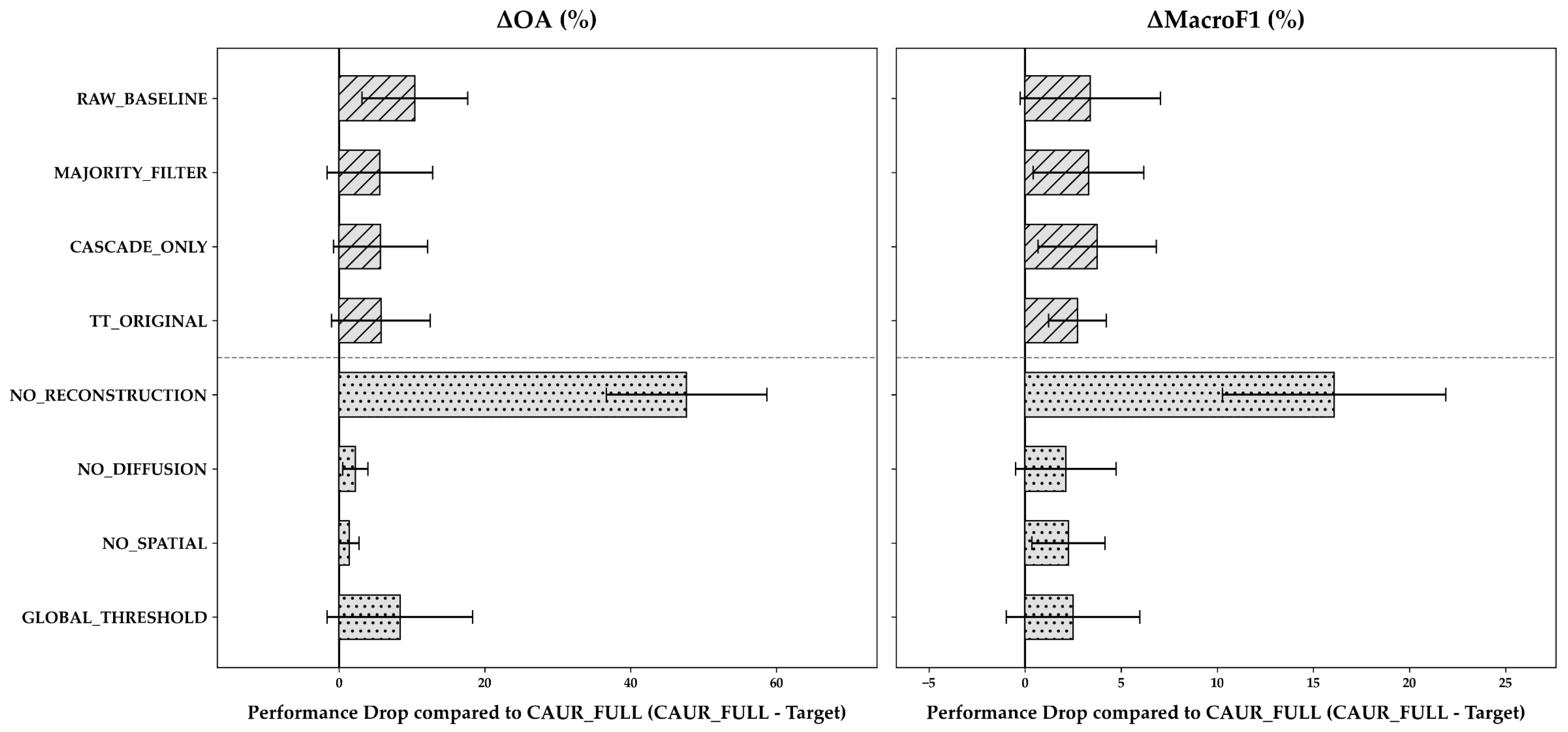
To verify the generality of these component contributions beyond tree-based ensembles, a supplementary 3-fold ablation control experiment was conducted using kNN across all seven datasets (Appendix D, Figure A2). The kNN results showed consistent behavioral trends. NO_RECONSTRUCTION caused the largest performance degradation (OA drop of +47.67%, p = 0.016, and Macro-F1 drop of +16.10%, p = 0.016), and GLOBAL_THRESHOLD led to substantial Macro-F1 degradation. Notably, the performance gap between CAUR_FULL and CASCADE_ONLY was smaller for kNN than for RF, while the net accuracy improvement from CAUR was more pronounced for kNN. These findings confirm that the internal mechanisms of CAUR operate effectively across diverse classifier types.
4. Discussion
4.1. Performance Dependencies on Dataset Constraints
Consistent with previous studies [81,82], the classifier’s performance in HS–MS complementary mapping largely depended on dataset characteristics. However, the strict confinement of training samples to the narrow HS–MS overlap region introduces unique challenges not captured by general comparisons. Therefore, the suitability of classification algorithms should be interpreted in the context of these strict spatial constraints.
Under such constraints, performance outcomes among the deep spatial–spectral architectures differed markedly between 3D-CNN and U-Net. 3D-CNN achieved the highest baseline performance across most datasets, consistent with its ability to extract localized spectral–spatial features from small three-dimensional patches. U-Net, in contrast, approached chance-level accuracy on the LULC datasets. One possible explanation is that encoder–decoder architectures like U-Net benefit substantially from spatially diverse training samples. Under the spatial confinement of the overlap region, the available training patches might not provide sufficient class-boundary diversity, limiting generalization [41]. These results suggest that patch-based architectures tend to be more effective when the spatial receptive field utilized by the model aligns well with the limited spatial extent of the HS–MS overlap region.
Conversely, lightweight pixel-wise classifiers, particularly RF variants [70,71,72,73], TabNet, and kNN, exhibited robust and stable performance across both tasks. This stability is consistent with the robustness of ensemble learning and distance-based classification under limited training conditions [83]. These observations suggest that lightweight pixel-wise classifiers provide a practical foundation for HS-MS complementary mapping. The primary remaining weakness of these classifiers (spatial inconsistency) can be effectively addressed through lightweight post-processing such as CAUR.
4.2. Design Implications of the Proposed Framework
The external comparison illustrates the structural trade-offs among different framework configurations (Figure 7). In the Cuprite dataset, TT_ORIGINAL achieved the highest OA. This higher accuracy is likely attributable to mineral-specific Band Math features [34]. In tree-based ensemble models, incorporating informative domain-specific features expands the feature space and facilitates forming more effective decision boundaries between classes [83].
In contrast, CASCADE_ONLY applies the cascade structure without these domain-specific features. While it improved Macro-F1, this configuration decreased OA compared to the baseline. These results indicate that while the cascade structure effectively isolates minority classes, it carries an inherent risk of propagating initial classification errors into subsequent classification stages. Conversely, TT_ORIGINAL is thought to mitigate such degradation because domain-specific features maintain a high initial classification accuracy.
Furthermore, the cascade structure’s efficacy depends on the base classifier. In the kNN control experiment (Appendix D, Figure A2), the performance gap between CAUR_FULL and CASCADE_ONLY was smaller than with RF. The most likely reason for this is that kNN relies on local distance relationships, so sequential class masking is likely to improve classification accuracy by excluding competing nearest neighbors from other classes. In contrast, RF resolves class boundaries natively through decision tree ensembles and therefore gains less additional benefit from external masking. This result indicates that cascade-style class masking can operate relatively effectively for kNN, though the extent of this effect may vary across datasets.
Ultimately, no single framework configuration is universally optimal. The preferred approach depends on the availability of domain-specific features and application requirements. When domain-specific features are available, incorporating them within a cascade framework appears most effective, as observed in the Cuprite experiments. When such features are unavailable, lightweight pixel-wise classifiers (such as RF or kNN) combined with CAUR provide a practical alternative with low computational cost and no classifier retraining. This conclusion is further supported by the consistent overall accuracy improvements observed across the Cuprite datasets (Section 4.3).
4.3. Mechanisms of CAUR: Balancing Spatial Coherence and Class Discrimination
The ablation analysis (Figure 7, Group 2) clarifies why CAUR behaves differently from a simple spatial majority filter. The first key mechanism is the class-adaptive threshold. Replacing it with a single global threshold (GLOBAL_THRESHOLD) reduced Macro-F1 while leaving OA largely unchanged. Because prediction uncertainty varies structurally among classes owing to differences in spectral separability [44], a single global threshold treats these distributions uniformly. Consequently, it risks over-revoking predictions in ambiguous classes while insufficiently revoking uncertain predictions in others. Class-adaptive thresholds address this mismatch, which accounts for mitigating the Macro-F1 degradation observed when evaluated against a global threshold.
The second mechanism is the spatial-isolation criterion. On average, removing this criterion (NO_SPATIAL) reduced performance relative to CAUR_FULL. However, at the individual fold level, NO_SPATIAL occasionally yielded a higher Macro-F1 score than CAUR_FULL because it unconditionally reconstructs all uncertain regions regardless of neighborhood agreement. Such unconditional smoothing risks overwriting genuinely correct isolated predictions. Therefore, we retain the spatial-isolation criterion to prevent over-smoothing and to protect valid class boundaries from being mistakenly overwritten.
The statistical analyses of the Cuprite datasets (Figure 8) further elucidate how the magnitude of CAUR’s effect varies across classifiers. In terms of overall accuracy, CAUR consistently improved performance across all 11 evaluated classifiers, yielding statistically significant gains for kNN, SVC, LR, MLP, GNB, and XGBoost. However, its effect on the Macro-F1 score was more variable. For instance, RF showed a significant improvement (+1.56%, p = 0.014), whereas XGBoost experienced a slight decrease (−0.91%, p = 0.030). These results highlight a clear trade-off: neighborhood reconstruction effectively removes pixel noise and improves overall accuracy, but it can also blur small or narrow patches of minority classes.
Figure 8.
Changes in overall accuracy (ΔOA) and macro-averaged F1-score (ΔMacro-F1) after applying CAUR relative to each baseline classifier across the five Cuprite reference datasets (AVIRIS–Hourglass, AVIRIS–Tetracorder, HISUI–Hourglass, EMIT–Hourglass, and EMIT–Tetracorder). Positive values indicate improvement over the baseline. The error bars represent the standard deviation of all datasets. Statistical significance from the Wilcoxon signed-rank test is indicated by asterisks (* p < 0.05, ** p < 0.01, *** p < 0.001).
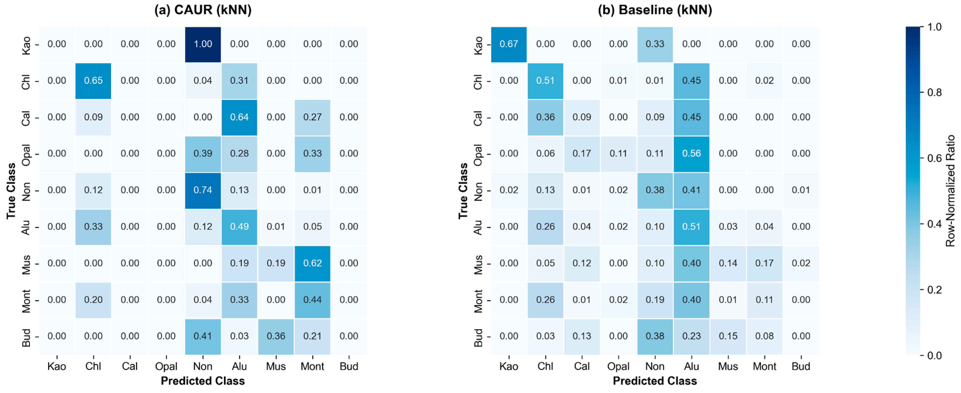
This trade-off is clearly demonstrated in the confusion matrix comparison for kNN on the Cuprite HISUI–Hourglass dataset (Figure A1, Appendix C). Applying CAUR markedly improved classification accuracy for spectrally confused minerals such as kaolinite, calcite, and opal, which were largely misclassified in the raw baseline. Conversely, montmorillonite precision decreased because its small, fragmented patches were merged into neighboring dominant classes during neighborhood reconstruction. Buddingtonite remained largely undetected under both configurations due to its limited pixel abundance across the test regions. Accordingly, CAUR should be regarded as a flexible post-classification module whose effectiveness and optimal pairing depend on both the underlying classifier and specific application requirements.
4.4. Practical Implications and Limitations
Sensor spatial resolution strongly influenced the practical effectiveness of the proposed framework. The accuracy improvements produced by CAUR were most pronounced on EMIT-derived datasets. Coarser spatial resolutions (such as EMIT’s 60 m) inherently increase the proportion of mixed pixels, which lowers classifier prediction confidence and generates scattered, high-entropy errors. CAUR mitigates this resolution-induced uncertainty by selectively identifying isolated ambiguous pixels and reconstructing them using confident spatial context. Although experimental factors such as class count varied between sensors, baseline accuracies remained comparable across AVIRIS, HISUI, and EMIT. This comparability suggests that the substantial improvements observed on EMIT are largely attributable to CAUR’s capability to effectively mitigate mixed-pixel artifacts in coarser-resolution imagery.
Methodological and statistical limitations also warrant consideration. First, deep neural networks were trained using single random seeds owing to computational constraints. Because repeated experiments across multiple random seeds and alternative data-partition settings [84,85] were not conducted, the reported performance may reflect stochastic variability associated with initialization and optimization. Second, the Wilcoxon signed-rank tests treated dataset-fold combinations as sampling units without family-wise error rate corrections [81], meaning statistical results should be viewed as indicative of performance trends rather than strict probabilistic bounds. Third, the component ablation analysis was verified across RF and kNN baselines. Whether the same component ranking holds for computationally intensive spatial–spectral deep neural networks (such as 3D-CNN and U-Net) cannot be assumed without further examination. Finally, the spatial reconstruction stage employs a fixed 3 × 3 neighborhood window, which risks over-smoothing fine linear structures in high-resolution data. Systematic evaluation of resolution-dependent performance degradation remains a topic for future research.
Several limitations regarding data characteristics and evaluation scope should also be highlighted. First, reference maps were generated using automated hyperspectral algorithms (Hourglass and Tetracorder) without independent field ground truth. Unquantified labeling errors in these reference products may affect baseline accuracy evaluations. Second, acquisition date discrepancies between HS and MS sensors (spanning 15 to 18 years for post-2008 Cuprite pairings and approximately 3 years for the Mito EMIT-ASTER pair) may have introduced spectral uncertainties that could not be independently isolated. Third, since evaluation was conducted via spatial holdout cross-validation within the HS–MS overlap area, while multispectral feature consistency across the scene was quantitatively confirmed (Section 2.3.1), direct empirical validation of inference in expansive MS areas outside the HS swath was precluded by the absence of reference labels and remains an inherent limitation of this study.
5. Conclusions
This study presents a flexible framework for HS-MS complementary mapping, addressing the lack of systematic classifier benchmarks and the trade-off between spatial consistency and computational efficiency. Through comprehensive evaluations of 13 classifiers across mineral and LULC mapping tasks, we demonstrated that classifier suitability is fundamentally governed by computational resources and training data constraints. When sufficient computational capacity is available, 3D-CNN achieves superior accuracy by learning joint spatial–spectral representations. Under computational constraints, lightweight classifiers such as RF and kNN provide robust, highly efficient baselines that serve as practical backbones for large-scale mapping.
To overcome the spatial fragmentation inherent in pixel-wise classifiers, we introduced CAUR as a lightweight, classifier-independent post-processing module. CAUR improves spatial coherence and classification accuracy without requiring model retraining and shows its greatest utility on coarser-resolution datasets where mixed-pixel uncertainty is prevalent. Component ablation confirmed that combining class-adaptive entropy thresholds with local spatial-isolation filtering is essential for balancing overall accuracy with minority-class preservation. In addition, comparative analysis showed that cascade structures provide tangible benefits only when paired with domain-specific diagnostic features. This finding indicates that cascade processing should be treated as an optional, domain-dependent module rather than a mandatory component.
Synthesizing these findings, this work provides practical design guidelines (Figure 9) for selecting optimal HS–MS mapping pipelines according to application goals, sensor resolutions, and computational budgets. Future research will explore adaptive neighborhood reconstruction techniques that dynamically preserve fine linear structures, extend the framework to multi-temporal HS–MS series to enforce temporal consistency, and integrate class-adaptive thresholding with semi-supervised learning to accommodate weak or noisy reference labels.
Figure 9.
Practical design guidelines for selecting appropriate classification pipelines in HS–MS complementary mapping. The optimal framework configuration is determined based on computational resources, the availability of domain-specific features, and the importance of preserving fine-scale spatial structures in high-resolution data.
Author Contributions
Conceptualization, H.T. (Hideyuki Tonooka); methodology, H.T. (Hideki Tsubomatsu) and H.T. (Hideyuki Tonooka); software, H.T. (Hideki Tsubomatsu); validation, H.T. (Hideki Tsubomatsu); formal analysis, H.T. (Hideki Tsubomatsu); investigation, H.T. (Hideki Tsubomatsu); resources, H.T. (Hideki Tsubomatsu) and H.T. (Hideyuki Tonooka); data curation, H.T. (Hideki Tsubomatsu); writing—original draft preparation, H.T. (Hideki Tsubomatsu); writing—review and editing, S.Y. and H.T. (Hideyuki Tonooka); visualization, H.T. (Hideki Tsubomatsu); supervision, S.Y. and H.T. (Hideyuki Tonooka); project administration, H.T. (Hideyuki Tonooka); funding acquisition, H.T. (Hideki Tsubomatsu) and H.T. (Hideyuki Tonooka). All authors have read and agreed to the published version of the manuscript.
Funding
This work was conducted with support from the Japan Science and Technology Agency (JST) SPRING Program (Grant Number JPMJSP2161).
Data Availability Statement
The code used in this study is available on GitHub (https://github.com/tsubomax/CAUR, v1.0 (accessed on 26 August 2026)); see the README.md for details. Tetracorder is also available on GitHub (https://github.com/PSI-edu/spectroscopy-tetracorder (accessed on 26 August 2026)). AVIRIS data are publicly available from the NASA AVIRIS Data Portal (https://aviris.jpl.nasa.gov/dataportal/ (accessed on 26 August 2026)). ASTER and EMIT data are available from the NASA EARTHDATA Portal (https://search.earthdata.nasa.gov/ (accessed on 26 August 2026)). HISUI data can be obtained through the Tellus platform (https://www.tellusxdp.com/ (accessed on 26 August 2026)).
Acknowledgments
The authors gratefully acknowledge Roger Clark of the U.S. Geological Survey for his assistance in the implementation of Tetracorder.
Conflicts of Interest
The authors declare no conflicts of interest. The funders had no role in the design of the study; in the collection, analyses, or interpretation of data; in the writing of the manuscript; or in the decision to publish the results.
Abbreviations
The following abbreviations are the primary ones used in this manuscript:
| CAUR | Class-adaptive uncertainty revocation |
| EPF | Edge-preserving filter |
| GNB | Gaussian naive Bayes |
| HS | Hyperspectral |
| LR | Logistic regression |
| LULC | Land use and land cover |
| MLP | Multi-layer perceptron |
| MS | Multispectral |
| OOB | Out-of-bag |
| OvR | One-vs-rest |
| RF | Random forest |
| SVC | Support vector machine |
| TT | Tsubomatsu–Tonooka |
Appendix A
Table A1 provides the implementation frameworks, network architectures, and Optuna Bayesian optimization search spaces for all 13 baseline classifiers and the CAUR module evaluated in this study.
Table A1.
Details of the implementation and Optuna hyperparameter search spaces for the evaluated classifiers and the CAUR module.
Appendix B
Table A2 and Table A3 present the classwise F1-scores (mean ± standard deviation across four spatial holdout folds, expressed as percentages) for the Cuprite HISUI–Hourglass (mineral mapping) and Mito HISUI–Hourglass (LULC mapping) datasets, respectively. Six representative configurations are shown: RF, CAUR(RF), kNN, CAUR(kNN), 3D-CNN, and CAUR(3D-CNN).
Table A2.
Classwise F1-scores (mean ± std, %) for the Cuprite HISUI–Hourglass dataset (9 mineral classes).
Table A3.
Classwise F1-scores (mean ± std, %) for the Mito HISUI–Hourglass dataset (12 LULC classes).
Appendix C
Figure A1 presents the normalized confusion matrices for the Cuprite HISUI–Hourglass dataset under kNN classification, comparing the CAUR-enhanced predictions (a) with the raw baseline predictions (b). This comparison highlights the resolution of severe salt-and-pepper noise for classes such as kaolinite, calcite, and opal, alongside the spatial merging of montmorillonite patches.
Figure A1.
Normalized confusion matrices for the Cuprite HISUI–Hourglass dataset under kNN classification: (a) CAUR (kNN); (b) baseline (kNN). Color bar indicates the normalized classification proportion [0.0, 1.0].
Appendix D
To verify the generality of CAUR’s component contributions across classifiers, an ablation control experiment was conducted using kNN as the base classifier across all seven datasets (Figure A2). Consistent with the results from the random forest (Section 3.2, Figure 7), neighborhood reconstruction and class-adaptive thresholding remain the primary drivers of performance improvements, confirming consistent functional synergy for distance-based classifiers.
Figure A2.
Framework comparison and component ablation using kNN as the base classifier across the seven reference datasets (3-fold cross-validation). Layout and conventions are identical to those in Figure 7.
References
- Schowengerdt, R.A. Remote Sensing: Models and Methods for Image Processing, 3rd ed.; Academic Press: Burlington, MA, USA, 2007. [Google Scholar]
- Foody, G.M. Status of Land Cover Classification Accuracy Assessment. Remote Sens. Environ. 2002, 80, 185–201. [Google Scholar] [CrossRef] [Scilit]
- Wulder, M.A.; Loveland, T.R.; Roy, D.P.; Crawford, C.J.; Masek, J.G.; Woodcock, C.E.; Allen, R.G.; Anderson, M.C.; Belward, A.S.; Cohen, W.B.; et al. Current Status of Landsat Program, Science, and Applications. Remote Sens. Environ. 2019, 225, 127–147. [Google Scholar] [CrossRef] [Scilit]
- Shaw, G.A.; Burke, H.K. Spectral Imaging for Remote Sensing. Linc. Lab. J. 2003, 14, 3–28. [Google Scholar]
- Li, P.; Jiang, L.; Feng, Z. Cross-Comparison of Vegetation Indices Derived from Landsat-7 Enhanced Thematic Mapper Plus (ETM+) and Landsat-8 Operational Land Imager (OLI) Sensors. Remote Sens. 2014, 6, 310–329. [Google Scholar] [CrossRef] [Scilit]
- Samadzadegan, F.; Toosi, A.; Dadrass Javan, F. A Critical Review on Multi-Sensor and Multi-Platform Remote Sensing Data Fusion Approaches: Current Status and Prospects. Int. J. Remote Sens. 2025, 46, 1327–1402. [Google Scholar] [CrossRef] [Scilit]
- Abrams, M.; Hook, S.; Ramachandran, B. ASTER User Handbook Version 2; NASA Goddard Space Flight Center: Greenbelt, MD, USA, 2002. [Google Scholar]
- Abrams, M.; Yamaguchi, Y. Twenty Years of ASTER Contributions to Lithologic Mapping and Mineral Exploration. Remote Sens. 2019, 11, 1394. [Google Scholar] [CrossRef] [Scilit]
- Rowan, L.C.; Hook, S.J.; Abrams, M.J.; Mars, J.C. Mapping Hydrothermally Altered Rocks at Cuprite, Nevada, Using the Advanced Spaceborne Thermal Emission and Reflection Radiometer (ASTER), a New Satellite-Imaging System. Econ. Geol. 2003, 98, 1019–1027. [Google Scholar] [CrossRef]
- Clark, R.N. Spectroscopy of Rocks and Minerals, and Principles of Spectroscopy. In Manual of Remote Sensing: Remote Sensing for the Earth Sciences; Rencz, A.N., Ed.; John Wiley & Sons: New York, NY, USA, 1999; Volume 3, pp. 3–58. [Google Scholar]
- Sabins, F.F. Remote Sensing for Mineral Exploration. Ore Geol. Rev. 1999, 14, 157–183. [Google Scholar] [CrossRef] [Scilit]
- Cudahy, T. Mineral Mapping for Exploration: An Australian Journey of Evolving Spectral Sensing Technologies and Industry Collaboration. Geosciences 2016, 6, 52. [Google Scholar] [CrossRef] [Scilit]
- Govender, M.; Chetty, K.; Bulcock, H. A Review of Hyperspectral Remote Sensing and Its Application in Vegetation and Water Resource Studies. Water SA 2007, 33, 145–151. [Google Scholar] [CrossRef] [Scilit]
- van der Meer, F.D.; van der Werff, H.M.A.; van Ruitenbeek, F.J.A.; Hecker, C.A.; Bakker, W.H.; Noomen, M.F.; van der Meijde, M.; Carranza, E.J.M.; de Smeth, J.B.; Woldai, T. Multi- and Hyperspectral Geologic Remote Sensing: A Review. Int. J. Appl. Earth Obs. Geoinf. 2012, 14, 112–128. [Google Scholar] [CrossRef] [Scilit]
- Green, R.O.; Eastwood, M.L.; Sarture, C.M.; Chrien, T.G.; Aronsson, M.; Chippendale, B.J.; Faust, J.A.; Pavri, B.E.; Chovit, C.J.; Solis, M.; et al. Imaging Spectroscopy and the Airborne Visible/Infrared Imaging Spectrometer (AVIRIS). Remote Sens. Environ. 1998, 65, 227–248. [Google Scholar] [CrossRef] [Scilit]
- Schaepman, M.E.; Jehle, M.; Hueni, A.; D’Odorico, P.; Damm, A.; Weyermann, J.; Schneider, F.D.; Laurent, V.; Popp, C.; Seidel, F.C.; et al. Advanced Radiometry Measurements and Earth Science Applications with the Airborne Prism Experiment (APEX). Remote Sens. Environ. 2015, 158, 207–219. [Google Scholar] [CrossRef] [Scilit]
- Guanter, L.; Kaufmann, H.; Segl, K.; Foerster, S.; Rogass, C.; Chabrillat, S.; Kuester, T.; Hollstein, A.; Rossner, G.; Chlebek, C.; et al. The EnMAP Spaceborne Imaging Spectroscopy Mission for Earth Observation. Remote Sens. 2015, 7, 8830–8857. [Google Scholar] [CrossRef] [Scilit]
- Pignatti, S.; Palombo, A.; Pascucci, S.; Romano, F.; Santini, F.; Simoniello, T.; Amato, U.; Cuomo, V.; Acito, N.; Diani, M.; et al. The PRISMA Hyperspectral Mission: Science Activities and Opportunities for Agriculture and Land Monitoring. In Proceedings of the 2013 IEEE International Geoscience and Remote Sensing Symposium (IGARSS 2013), Melbourne, VIC, Australia, 21–26 July 2013; IEEE: Piscataway, NJ, USA, 2013; pp. 4558–4561. [Google Scholar] [CrossRef] [Scilit]
- Matsunaga, T.; Iwasaki, A.; Tsuchida, S.; Iwao, K.; Tanii, J.; Kashimura, O.; Nakamura, R.; Yamamoto, H.; Kato, S.; Obata, K.; et al. Current Status of the Hyperspectral Imager Suite (HISUI). In Proceedings of the 2017 IEEE International Geoscience and Remote Sensing Symposium (IGARSS 2017), Fort Worth, TX, USA, 23–28 July 2017; pp. 443–446. [Google Scholar] [CrossRef] [Scilit]
- Tanii, J.; Kashimura, O.; Ito, Y.; Iwasaki, A. Flight Model Performances of HISUI Hyperspectral Sensor Onboard ISS (International Space Station). In Proceedings of SPIE 10000, Sensors, Systems, and Next-Generation Satellites XX, Edinburgh, UK, 26–29 September 2016; SPIE: Bellingham, WA, USA, 2016; p. 100000A. [Google Scholar] [CrossRef] [Scilit]
- Iwasaki, A.; Tanii, J.; Kashimura, O.; Ito, Y. Prelaunch Status of Hyperspectral Imager Suite (HISUI). In Proceedings of the 2019 IEEE International Geoscience and Remote Sensing Symposium (IGARSS 2019), Yokohama, Japan, 28 July–2 August 2019; IEEE: Piscataway, NJ, USA, 2019; pp. 9070–9072. [Google Scholar] [CrossRef] [Scilit]
- Mizuochi, H.; Tsuchida, S.; Yamamoto, S.; Urai, M.; Matsuoka, M.; Ikeda, A.; Iwao, K. First Cross- and Inter-Band Calibrations of the Hyperspectral Imager Suite Using Off-Nadir Quasi-Simultaneous Overpass Counterparts. IEEE Trans. Geosci. Remote Sens. 2024, 62, 5527517. [Google Scholar] [CrossRef] [Scilit]
- Green, R.O.; Mahowald, N.; Ung, C.; Thompson, D.R.; Bator, L.; Bennet, M.; Bernas, M.; Blackway, N.; Bradley, C.; Cha, J.; et al. The Earth Surface Mineral Dust Source Investigation: An Earth Science Imaging Spectroscopy Mission. In Proceedings of the 2020 IEEE Aerospace Conference, Big Sky, MT, USA, 7–14 March 2020; IEEE: Piscataway, NJ, USA, 2020; pp. 1–15. [Google Scholar] [CrossRef] [Scilit]
- Thompson, D.R.; Green, R.O.; Bradley, C.; Brodrick, P.G.; Mahowald, N.; Ben Dor, E.; Bennett, M.; Bernas, M.; Carmon, N.; Chadwick, K.D.; et al. On-Orbit Calibration and Performance of the EMIT Imaging Spectrometer. Remote Sens. Environ. 2024, 303, 113986. [Google Scholar] [CrossRef] [Scilit]
- Cawse-Nicholson, K.; Townsend, P.A.; Schimel, D.; Assiri, A.M.; Blake, P.L.; Buongiorno, M.F.; Campbell, P.K.E.; Carmon, N.; Casey, K.A.; Correa-Pabón, R.E.; et al. NASA’s Surface Biology and Geology Designated Observable: A Perspective on Surface Imaging Algorithms. Remote Sens. Environ. 2021, 257, 112349. [Google Scholar] [CrossRef] [Scilit]
- Rast, M.; Nieke, J.; Adams, J.; Isola, C.; Gascon, F. Copernicus Hyperspectral Imaging Mission for the Environment (CHIME). In Proceedings of the 2021 IEEE International Geoscience and Remote Sensing Symposium (IGARSS 2021), Brussels, Belgium, 11–16 July 2021; IEEE: Piscataway, NJ, USA, 2021; pp. 108–111. [Google Scholar] [CrossRef] [Scilit]
- Kruse, F.A.; Perry, S.L. Improving Multispectral Mineral Mapping Using Constrained Spectral Unmixing with AVIRIS-Derived Endmembers. In Proceedings of the Eleventh JPL Airborne Earth Science Workshop, Pasadena, CA, USA, 4–8 March 2002; Jet Propulsion Laboratory: Pasadena, CA, USA, 2002; pp. 217–226. [Google Scholar]
- Kruse, F.A.; Perry, S.L. Regional Mineral Mapping by Extending Hyperspectral Signatures Using Multispectral Data. In Proceedings of the 2007 IEEE Aerospace Conference, Big Sky, MT, USA, 3–10 March 2007; IEEE: Piscataway, NJ, USA, 2007; pp. 1–14. [Google Scholar] [CrossRef] [Scilit]
- Chander, G.; Markham, B.L.; Helder, D.L. Summary of Current Radiometric Calibration Coefficients for Landsat MSS, TM, ETM+, and EO-1 ALI Sensors. Remote Sens. Environ. 2009, 113, 893–903. [Google Scholar] [CrossRef] [Scilit]
- Adler-Golden, S.M.; Matthew, M.W.; Bernstein, L.S.; Levine, R.Y.; Berk, A.; Richtsmeier, S.C.; Acharya, P.K.; Anderson, G.P.; Felde, G.W.; Gardner, J.A.; et al. Atmospheric Correction for Short-Wave Spectral Imagery Based on MODTRAN4. In Proceedings of SPIE 3753, Imaging Spectrometry V, Denver, CO, USA, 18–23 July 1999; Descour, M.R., Shen, S.S., Eds.; SPIE: Bellingham, WA, USA, 1999; pp. 61–69. [Google Scholar] [CrossRef] [Scilit]
- Hirai, A.; Tonooka, H. Mineral discrimination by combination of multispectral image and surrounding hyperspectral image. J. Appl. Remote Sens. 2019, 13, 024517. [Google Scholar] [CrossRef] [Scilit]
- Townshend, J.R.G.; Justice, C.O.; Gurney, C.; McManus, J. The Impact of Misregistration on Change Detection. IEEE Trans. Geosci. Remote Sens. 1992, 30, 1054–1060. [Google Scholar] [CrossRef] [Scilit]
- Nakayama, K.; Tonooka, H. Improvement of a Mineral Discrimination Method Using Multispectral Image and Surrounding Hyperspectral Image. J. Appl. Remote Sens. 2021, 15, 044501. [Google Scholar] [CrossRef] [Scilit]
- Ni, L.; Zhang, B.; Gao, L.; Li, S.; Wu, Y. Optimising the Use of Hyperspectral and Multispectral Data for Regional Crop Classification. In Proceedings of SPIE 8745, Signal Processing, Sensor Fusion, and Target Recognition XXII, Baltimore, MD, USA, 29 April–3 May 2013; SPIE: Bellingham, WA, USA, 2013; p. 87451V. [Google Scholar] [CrossRef] [Scilit]
- Tsubomatsu, H.; Tonooka, H. Region Expansion of a Hyperspectral-Based Mineral Map Using Random Forest Classification with Multispectral Data. Minerals 2023, 13, 754. [Google Scholar] [CrossRef] [Scilit]
- Clark, R.N.; Swayze, G.A.; Livo, K.E.; Kokaly, R.F.; Sutley, S.J.; Dalton, J.B.; McDougal, R.R.; Gent, C.A. Imaging Spectroscopy: Earth and Planetary Remote Sensing with the USGS Tetracorder and Expert Systems. J. Geophys. Res. 2003, 108, 5131. [Google Scholar] [CrossRef] [Scilit]
- Gao, F.; Jin, X.; Zhou, X.; Dong, J.; Du, Q. MSFMamba: Multiscale Feature Fusion State Space Model for Multisource Remote Sensing Image Classification. IEEE Trans. Geosci. Remote Sens. 2025, 63, 5504116. [Google Scholar] [CrossRef] [Scilit]
- Wang, J.; Li, W.; Gao, Y.; Zhang, M.; Tao, R.; Du, Q. Hyperspectral and SAR Image Classification via Multiscale Interactive Fusion Network. IEEE Trans. Neural Netw. Learn. Syst. 2023, 34, 10823–10837. [Google Scholar] [CrossRef] [Scilit] [PubMed]
- Tang, M.; Cozma, A.; Georgiou, K.; Qi, H. Cross-Scale MAE: A Tale of Multiscale Exploitation in Remote Sensing. In Advances in Neural Information Processing Systems 36 (NeurIPS 2023); Oh, A., Naumann, T., Globerson, A., Saenko, K., Hardt, M., Levine, S., Eds.; Curran Associates, Inc.: Red Hook, NY, USA, 2023; pp. 20054–20066. [Google Scholar]
- Hirayama, H.; Sharma, R.C.; Tomita, M.; Hara, K. Evaluating Multiple Classifier System for the Reduction of Salt-and-Pepper Noise in the Classification of Very-High-Resolution Satellite Images. Int. J. Remote Sens. 2019, 40, 2542–2557. [Google Scholar] [CrossRef] [Scilit]
- Wambugu, N.; Chen, S.; Yang, M.; Wang, S. Hyperspectral Image Classification on Insufficient-Sample and Feature Learning Using Deep Neural Networks: A Review. Int. J. Appl. Earth Obs. Geoinf. 2021, 105, 102603. [Google Scholar] [CrossRef] [Scilit]
- Huang, X.; Lu, Q.; Zhang, L.; Plaza, A. New Postprocessing Methods for Remote Sensing Image Classification: A Systematic Study. IEEE Trans. Geosci. Remote Sens. 2014, 52, 7140–7159. [Google Scholar] [CrossRef] [Scilit]
- Wang, L.; Shi, C.; Diao, C.; Ji, W.; Yin, D. A Survey of Methods Incorporating Spatial Information in Image Classification and Spectral Unmixing. Int. J. Remote Sens. 2016, 37, 3870–3910. [Google Scholar] [CrossRef] [Scilit]
- Lu, Y.; Sun, P.; Linghu, L.; Zhang, M. Uncertainty Evaluation Approach Based on Shannon Entropy for Upscaled Land Use/Cover Maps. J. Land Use Sci. 2022, 17, 648–657. [Google Scholar] [CrossRef] [Scilit]
- Kim, K.E. Adaptive Majority Filtering for Contextual Classification of Remote Sensing Data. Int. J. Remote Sens. 1996, 17, 1083–1087. [Google Scholar] [CrossRef] [Scilit]
- Rivai, F.A.; Tjahjono, B.; Munibah, K. Majority Filter for Enhancing Pixel-Based Random Forest Land Cover Classification in Sukajaya District, Bogor Regency. Geogr. Environ. Sustain. 2025, 18, 171–182. [Google Scholar] [CrossRef] [Scilit]
- Dehghan, H.; Ghassemian, H. Measurement of Uncertainty by the Entropy: Application to the Classification of MSS Data. Int. J. Remote Sens. 2006, 27, 4005–4014. [Google Scholar] [CrossRef] [Scilit]
- Zhang, Q.; Zhang, P.; Hu, X. Novel Classification Uncertainty Measurement Model Integrating Spatial Information for Remote Sensing Image. ISPRS Ann. Photogramm. Remote Sens. Spat. Inf. Sci. 2020, V-3-2020, 723–730. [Google Scholar] [CrossRef] [Scilit]
- Kruse, F.A.; Kierein-Young, K.S.; Boardman, J.W. Mineral Mapping at Cuprite, Nevada with a 63-Channel Imaging Spectrometer. Photogramm. Eng. Remote Sens. 1990, 56, 83–92. [Google Scholar]
- Clark, R.N.; King, T.V.V.; Klejwa, M.; Swayze, G.A.; Vergo, N. High Spectral Resolution Reflectance Spectroscopy of Minerals. J. Geophys. Res. Solid Earth 1990, 95, 12653–12680. [Google Scholar] [CrossRef] [Scilit]
- Tsubomatsu, H.; Yamamoto, S.; Tonooka, H. Gap Filling in HISUI Hyperspectral Classification Maps Through Integration with ASTER Multispectral Data in Ibaraki Prefecture, Japan. In Proceedings of the International Symposium on Remote Sensing (ISRS) 2025, Incheon, Republic of Korea, 14–16 May 2025. [Google Scholar]
- NASA Jet Propulsion Laboratory. AVIRIS Data Portal. Available online: https://aviris.jpl.nasa.gov/dataportal/ (accessed on 17 August 2026).
- Johnson, K.E.; Koperski, K. VNIR-SWIR Superspectral Mineral Mapping: An Example from Cuprite, Nevada. Photogramm. Eng. Remote Sens. 2020, 86, 695–700. [Google Scholar] [CrossRef] [Scilit]
- Matthew, M.W.; Adler-Golden, S.M.; Berk, A.; Felde, G.W.; Anderson, G.P.; Gorodetzky, D.; Paswaters, S.; Shippert, M.; Hoke, M.L. Status of Atmospheric Correction Using a MODTRAN4-Based Algorithm. In Proceedings of SPIE 4049, Algorithms for Multispectral, Hyperspectral, and Ultraspectral Imagery VI, Orlando, FL, USA, 24–28 April 2000; Shen, S.S., Descour, M.R., Eds.; SPIE: Bellingham, WA, USA, 2000; pp. 199–207. [Google Scholar] [CrossRef] [Scilit]
- Green, A.A.; Berman, M.; Switzer, P.; Craig, M.D. A Transformation for Ordering Multispectral Data in Terms of Image Quality with Implications for Noise Removal. IEEE Trans. Geosci. Remote Sens. 1988, 26, 65–74. [Google Scholar] [CrossRef] [Scilit]
- Boardman, J.W.; Kruse, F.A.; Green, R.O. Mapping Target Signatures via Partial Unmixing of AVIRIS Data. In Summaries of the Fifth Annual JPL Airborne Earth Science Workshop, Pasadena, CA, USA, 23–26 January 1995; Green, R.O., Ed.; JPL Publication 95-1; Jet Propulsion Laboratory: Pasadena, CA, USA, 1995; Volume 1, pp. 23–26. [Google Scholar]
- Boardman, J.W.; Kruse, F.A. Analysis of Imaging Spectrometer Data Using N-Dimensional Geometry and a Mixture-Tuned Matched Filtering Approach. IEEE Trans. Geosci. Remote Sens. 2011, 49, 4138–4152. [Google Scholar] [CrossRef] [Scilit]
- Yuhas, R.H.; Goetz, A.F.H.; Boardman, J.W. Discrimination among Semi-Arid Landscape Endmembers Using the Spectral Angle Mapper (SAM) Algorithm. In Summaries of the Third Annual JPL Airborne Geoscience Workshop, Pasadena, CA, USA, 1–5 June 1992; Green, R.O., Ed.; JPL Publication 92-14; Jet Propulsion Laboratory: Pasadena, CA, USA, 1992; Volume 1, pp. 148–150. [Google Scholar]
- Clark, R.N.; Swayze, G.A.; Livo, K.E.; Brodrick, P.G.; Dobrea, E.N.; Vijayarangan, S.; Green, R.O.; Wettergreen, D.; Candela, A.; Hendrix, A.; et al. The EMIT and TREX teams. Imaging Spectroscopy: Earth and Planetary Remote Sensing with the PSI Tetracorder and Expert Systems from Rovers to EMIT and Beyond. Planet. Sci. J. 2024, 5, 276. [Google Scholar] [CrossRef] [Scilit]
- Google LLC. Google Maps. Available online: https://www.google.com/maps (accessed on 17 August 2026).
- John, G.H.; Langley, P. Estimating Continuous Distributions in Bayesian Classifiers. In Proceedings of the Eleventh Conference on Uncertainty in Artificial Intelligence (UAI ‘95), Montreal, QC, Canada, 18–20 August 1995; Besnard, P., Hanks, S., Eds.; Morgan Kaufmann Publishers Inc.: San Francisco, CA, USA, 1995; pp. 338–345. [Google Scholar]
- Cover, T.; Hart, P. Nearest Neighbor Pattern Classification. IEEE Trans. Inf. Theory 1967, 13, 21–27. [Google Scholar] [CrossRef] [Scilit]
- Das, P.; Pandey, A.C. Land Use/Land Cover Classification Using Logistic Regression Based on Optimal Training Dataset Generated from Ground Truth. J. Indian Soc. Remote Sens. 2019, 47, 1835–1843. [Google Scholar] [CrossRef] [Scilit]
- Rumelhart, D.E.; Hinton, G.E.; Williams, R.J. Learning Representations by Back-Propagating Errors. Nature 1986, 323, 533–536. [Google Scholar] [CrossRef] [Scilit]
- Cortes, C.; Vapnik, V. Support-Vector Networks. Mach. Learn. 1995, 20, 273–297. [Google Scholar] [CrossRef] [Scilit]
- Hu, W.; Huang, Y.; Wei, L.; Zhang, Z.; Li, H. Deep Convolutional Neural Networks for Hyperspectral Image Classification. J. Sens. 2015, 2015, 258619. [Google Scholar] [CrossRef] [Scilit]
- Arik, S.Ö.; Pfister, T. TabNet: Attentive Interpretable Tabular Learning. In Proceedings of the AAAI Conference on Artificial Intelligence, Virtual Event, 2–9 February 2021; AAAI Press: Palo Alto, CA, USA, 2021; Volume 35, pp. 6679–6687. [Google Scholar] [CrossRef] [Scilit]
- Yang, X.; Zhang, X.; Ye, Y.; Lau, R.Y.K.; Lu, S.; Li, X.; Huang, X. Synergistic 2D/3D Convolutional Neural Network for Hyperspectral Image Classification. Remote Sens. 2020, 12, 2033. [Google Scholar] [CrossRef] [Scilit]
- Ronneberger, O.; Fischer, P.; Brox, T. U-Net: Convolutional Networks for Biomedical Image Segmentation. In Proceedings of the International Conference on Medical Image Computing and Computer-Assisted Intervention (MICCAI 2015), Munich, Germany, 5–9 October 2015; Navab, N., Hornegger, J., Wells, W.M., Frangi, A.F., Eds.; Springer: Cham, Switzerland, 2015; pp. 234–241. [Google Scholar] [CrossRef] [Scilit]
- Breiman, L. Random Forests. Mach. Learn. 2001, 45, 5–32. [Google Scholar] [CrossRef] [Scilit]
- Allwein, E.L.; Schapire, R.E.; Singer, Y. Reducing Multiclass to Binary: A Unifying Approach for Margin Classifiers. J. Mach. Learn. Res. 2000, 1, 113–141. [Google Scholar]
- Xia, J.; Dalla Mura, M.; Chanussot, J.; Du, P.; He, X. Spectral–Spatial Classification of Hyperspectral Images Using ICA and Edge-Preserving Filter via an Ensemble Strategy. IEEE Trans. Geosci. Remote Sens. 2016, 54, 4971–4982. [Google Scholar] [CrossRef] [Scilit]
- Chen, T.; Guestrin, C. XGBoost: A Scalable Tree Boosting System. In Proceedings of the 22nd ACM SIGKDD International Conference on Knowledge Discovery and Data Mining (KDD ‘16), San Francisco, CA, USA, 13–17 August 2016; Association for Computing Machinery: New York, NY, USA, 2016; pp. 785–794. [Google Scholar] [CrossRef] [Scilit]
- Akiba, T.; Sano, S.; Yanase, T.; Ohta, T.; Koyama, M. Optuna: A Next-Generation Hyperparameter Optimization Framework. In Proceedings of the 25th ACM SIGKDD International Conference on Knowledge Discovery & Data Mining (KDD ‘19), Anchorage, AK, USA, 4–8 August 2019; Association for Computing Machinery: New York, NY, USA, 2019; pp. 2623–2631. [Google Scholar] [CrossRef] [Scilit]
- Kuhn, S.; Cracknell, M.J.; Reading, A.M. Lithological Mapping Using Random Forests Applied to Geophysical and Remote Sensing Data: A Demonstration Study from the Eastern Goldfields of Australia. Geophysics 2018, 83, B183–B193. [Google Scholar] [CrossRef] [Scilit]
- Shadman Roodposhti, M.; Aryal, J.; Lucieer, A.; Bryan, B.A. Uncertainty Assessment of Hyperspectral Image Classification: Deep Learning vs. Random Forest. Entropy 2019, 21, 78. [Google Scholar] [CrossRef] [Scilit] [PubMed]
- Stefanski, J.; Mack, B.; Waske, B. Optimization of Object-Based Image Analysis with Random Forests for Land Cover Mapping. IEEE J. Sel. Top. Appl. Earth Obs. Remote Sens. 2013, 6, 2492–2504. [Google Scholar] [CrossRef] [Scilit]
- Cánovas-García, F.; Alonso-Sarría, F.; Gomariz-Castillo, F.; Oñate-Valdivieso, F. Modification of the Random Forest Algorithm to Avoid Statistical Dependence Problems When Classifying Remote Sensing Imagery. Comput. Geosci. 2017, 103, 1–11. [Google Scholar] [CrossRef] [Scilit]
- Pedregosa, F.; Varoquaux, G.; Gramfort, A.; Michel, V.; Thirion, B.; Grisel, O.; Blondel, M.; Prettenhofer, P.; Weiss, R.; Dubourg, V.; et al. Scikit-Learn: Machine Learning in Python. J. Mach. Learn. Res. 2011, 12, 2825–2830. [Google Scholar]
- Cui, Y.; Jia, M.; Lin, T.-Y.; Song, Y.; Belongie, S. Class-Balanced Loss Based on Effective Number of Samples. In Proceedings of the IEEE/CVF Conference on Computer Vision and Pattern Recognition (CVPR 2019), Long Beach, CA, USA, 15–20 June 2019; IEEE: Piscataway, NJ, USA, 2019; pp. 9260–9269. [Google Scholar] [CrossRef] [Scilit]
- Demšar, J. Statistical Comparisons of Classifiers over Multiple Data Sets. J. Mach. Learn. Res. 2006, 7, 1–30. [Google Scholar]
- McElfresh, D.; Khandagale, S.; Valverde, J.; Prasad, V.C.; Ramakrishnan, G.; Goldblum, M.; White, C. When Do Neural Nets Outperform Boosted Trees on Tabular Data? In Advances in Neural Information Processing Systems 36 (NeurIPS 2023); Oh, A., Naumann, T., Globerson, A., Saenko, K., Hardt, M., Levine, S., Eds.; Curran Associates, Inc.: Red Hook, NY, USA, 2023; pp. 76336–76369. [Google Scholar]
- Belgiu, M.; Drăguţ, L. Random Forest in Remote Sensing: A Review of Applications and Future Directions. ISPRS J. Photogramm. Remote Sens. 2016, 114, 24–31. [Google Scholar] [CrossRef] [Scilit]
- Wang, S. Temporal–Contextual Self-Supervised Time-Series Learning for Automated Fault Detection and Diagnosis of Air Handling Units in Buildings. Build. Environ. 2026, 292, 114300. [Google Scholar] [CrossRef] [Scilit]
- Wang, S. Class-Aware Temporal and Contextual Contrastive Framework for Semi-Supervised Automated Fault Detection and Diagnosis in Air Handling Units. Energy Build. 2026, 358, 117233. [Google Scholar] [CrossRef] [Scilit]
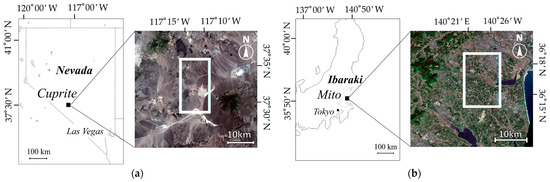
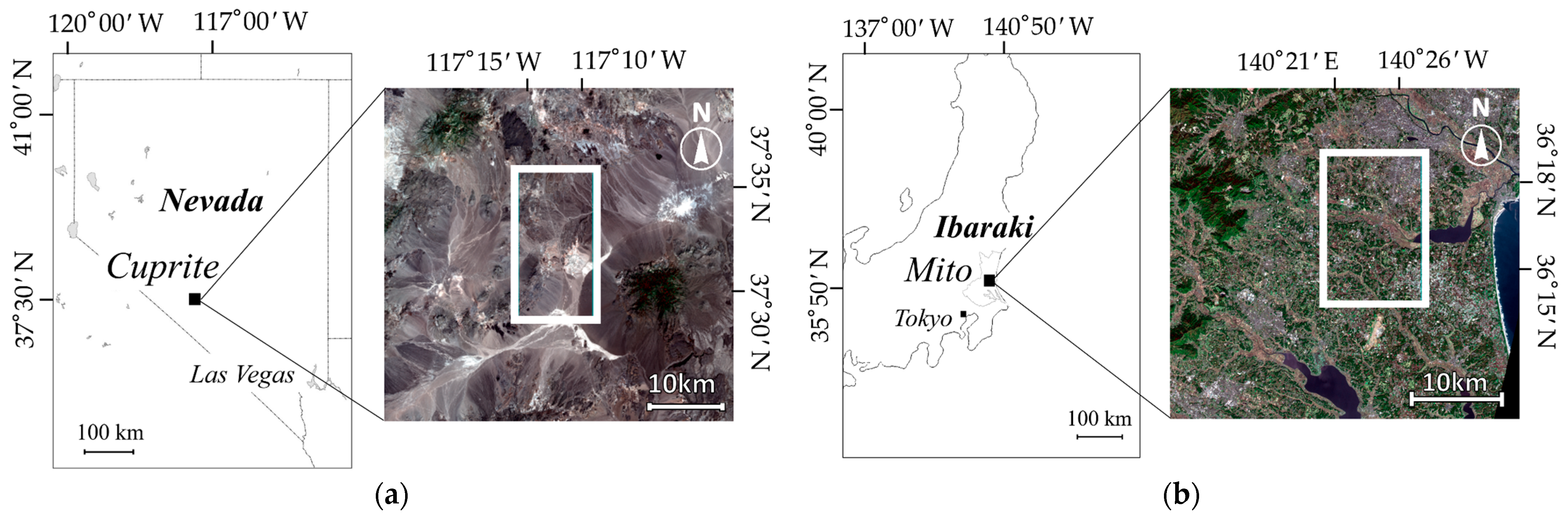
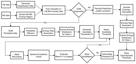
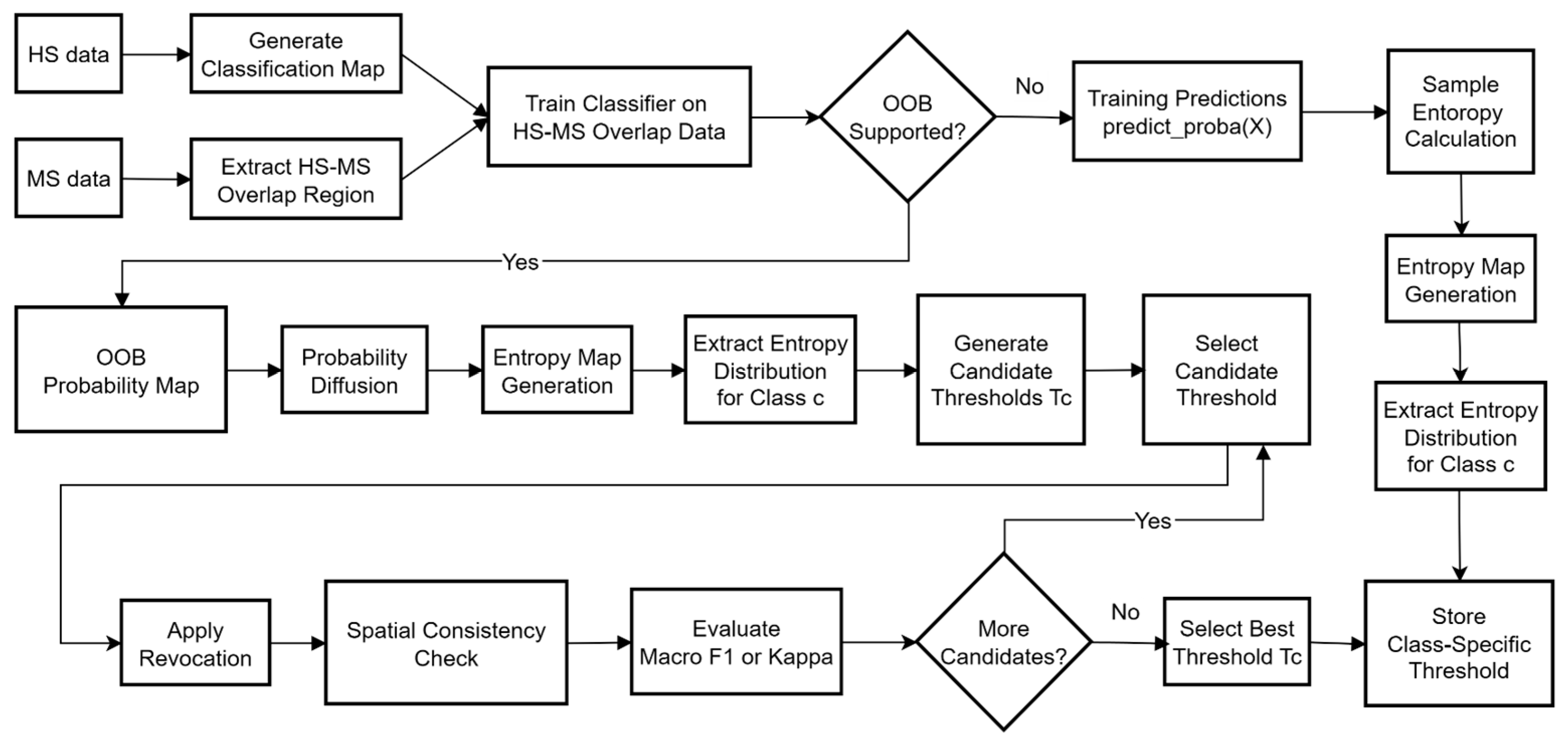
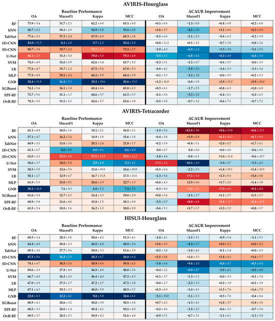
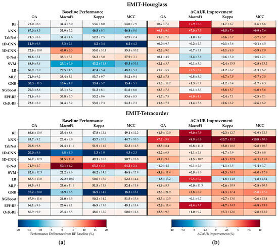
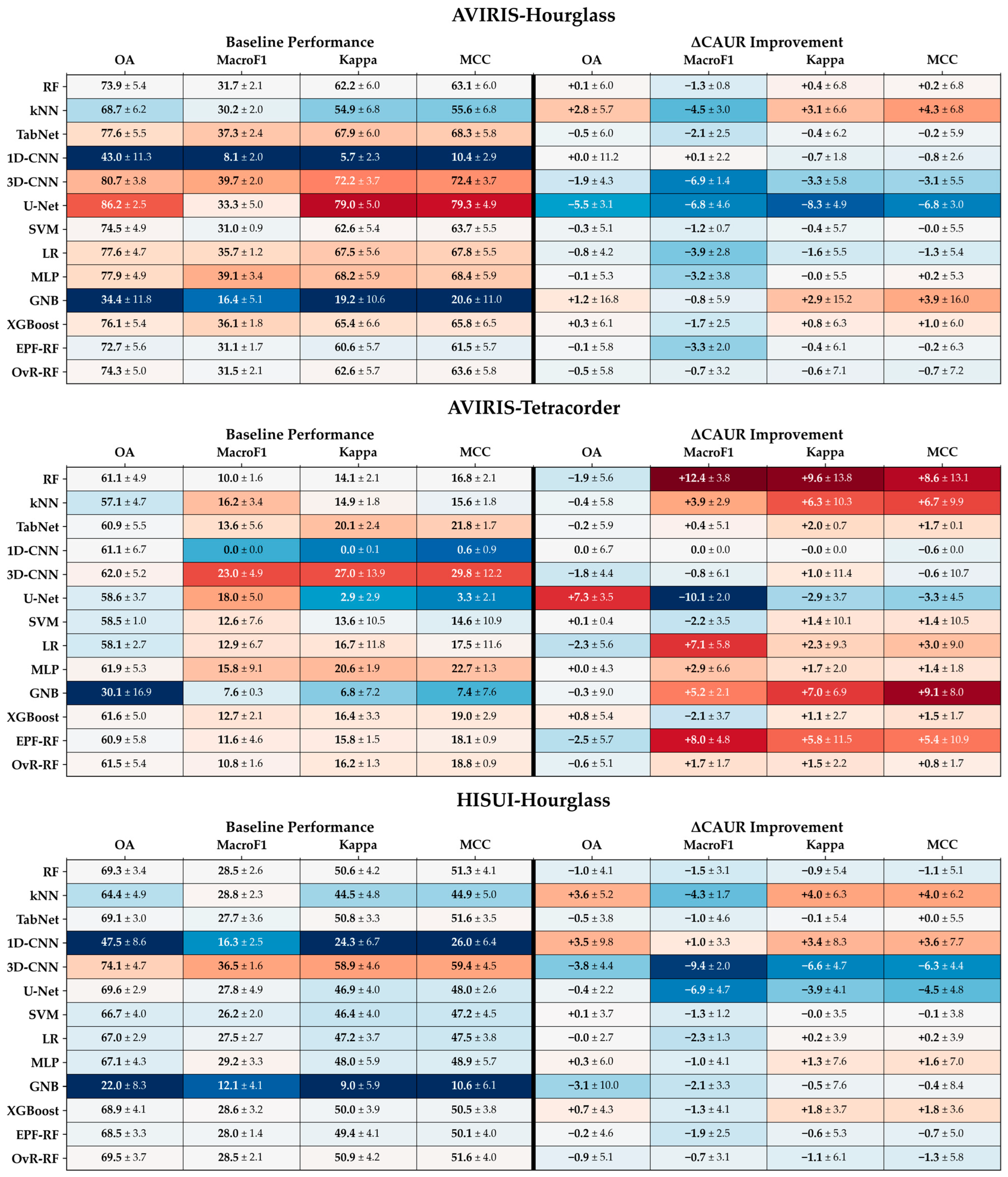
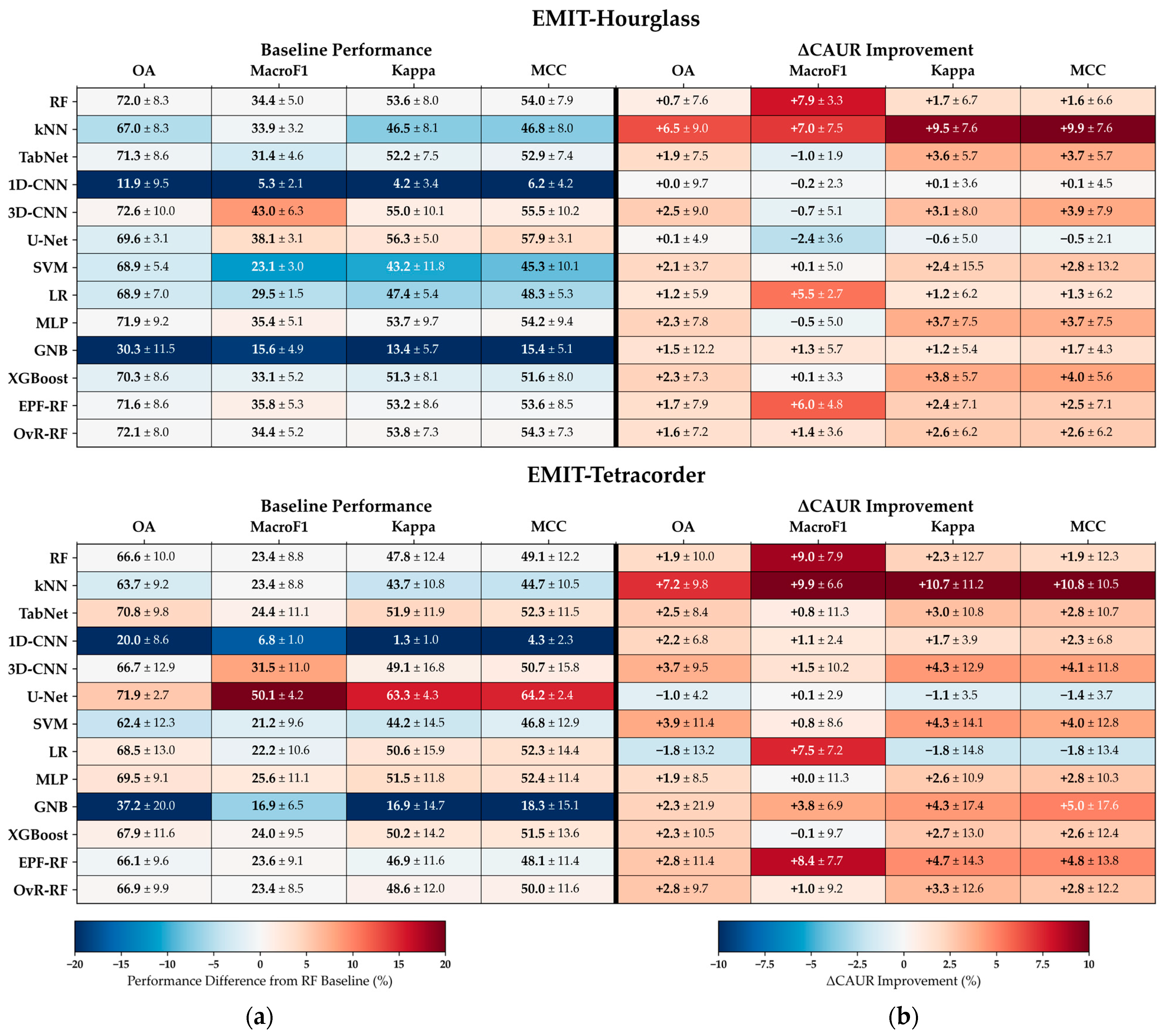
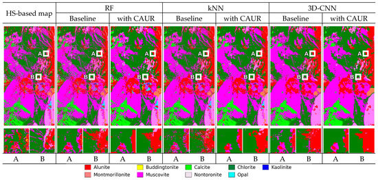
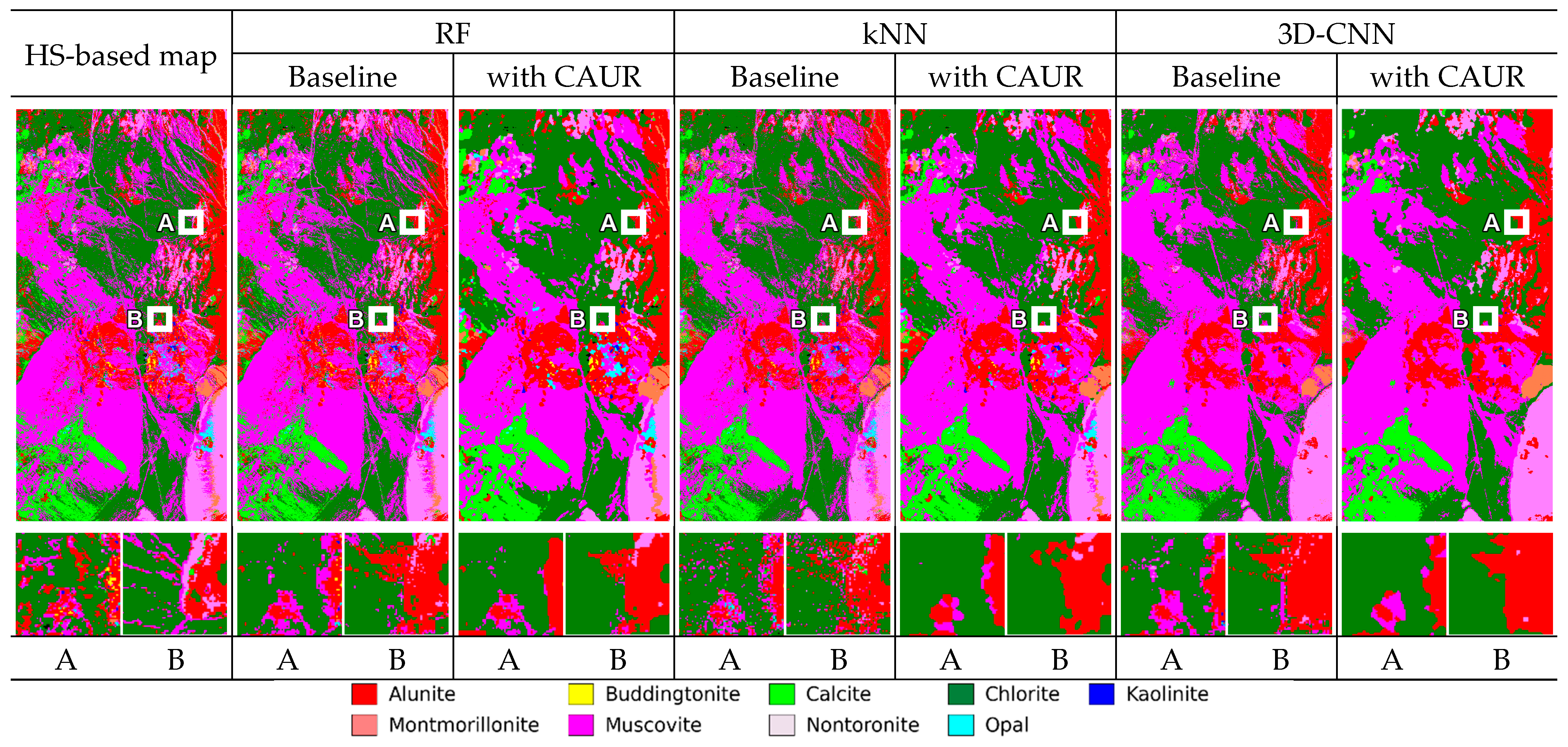
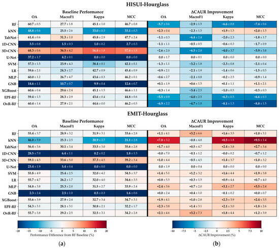
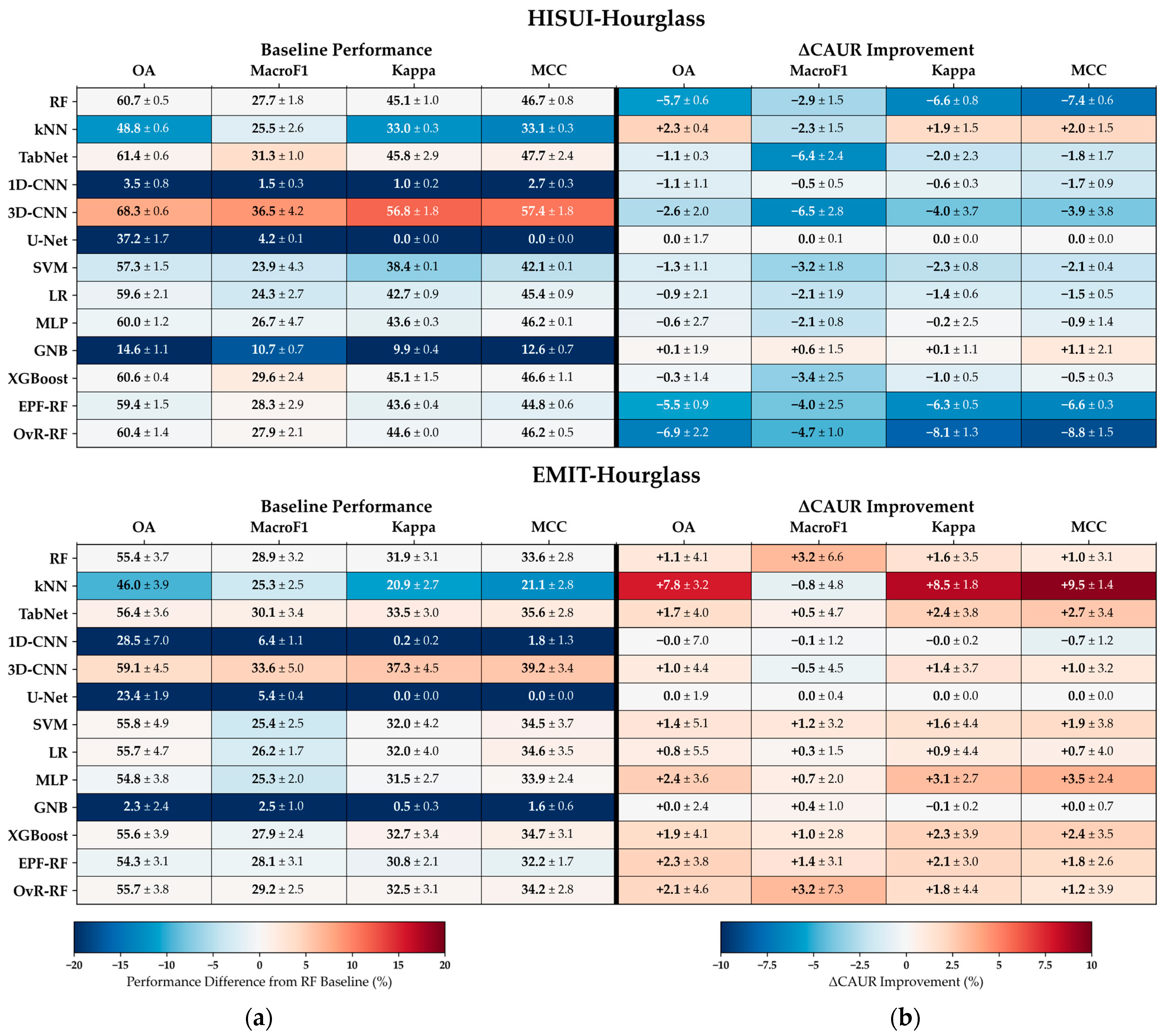
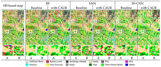
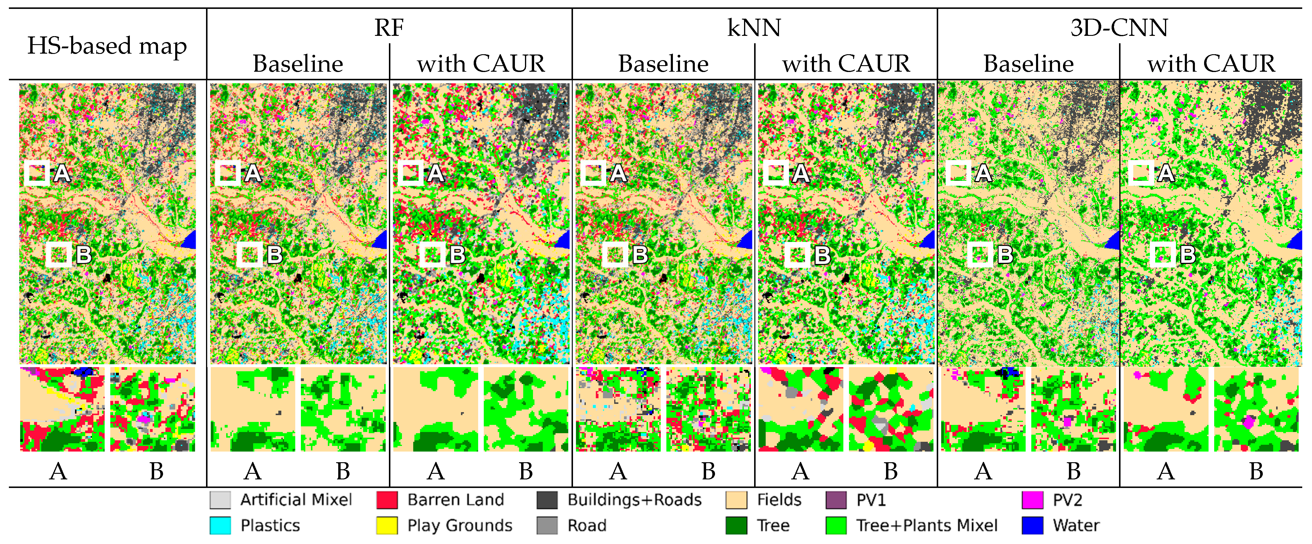
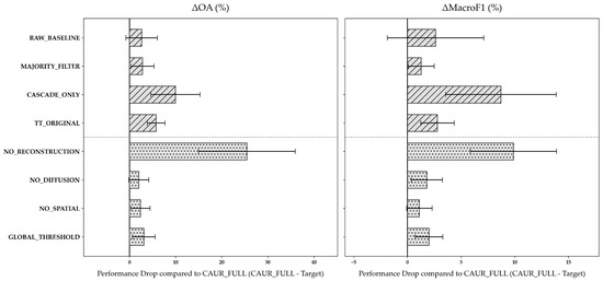
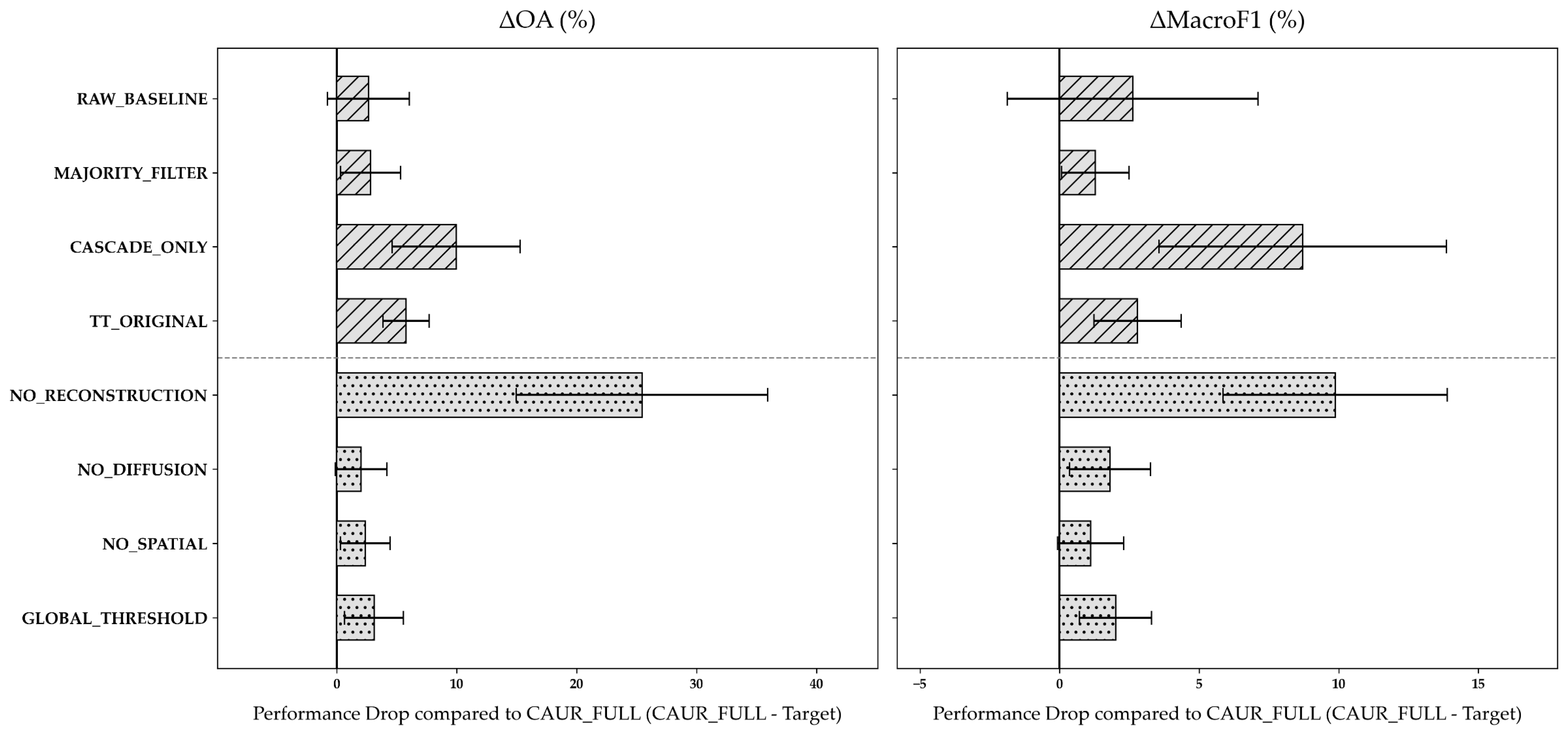
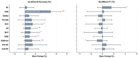
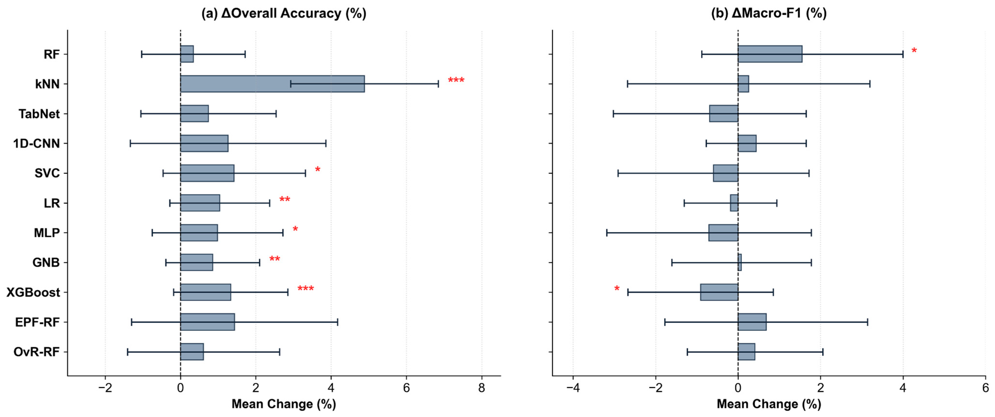
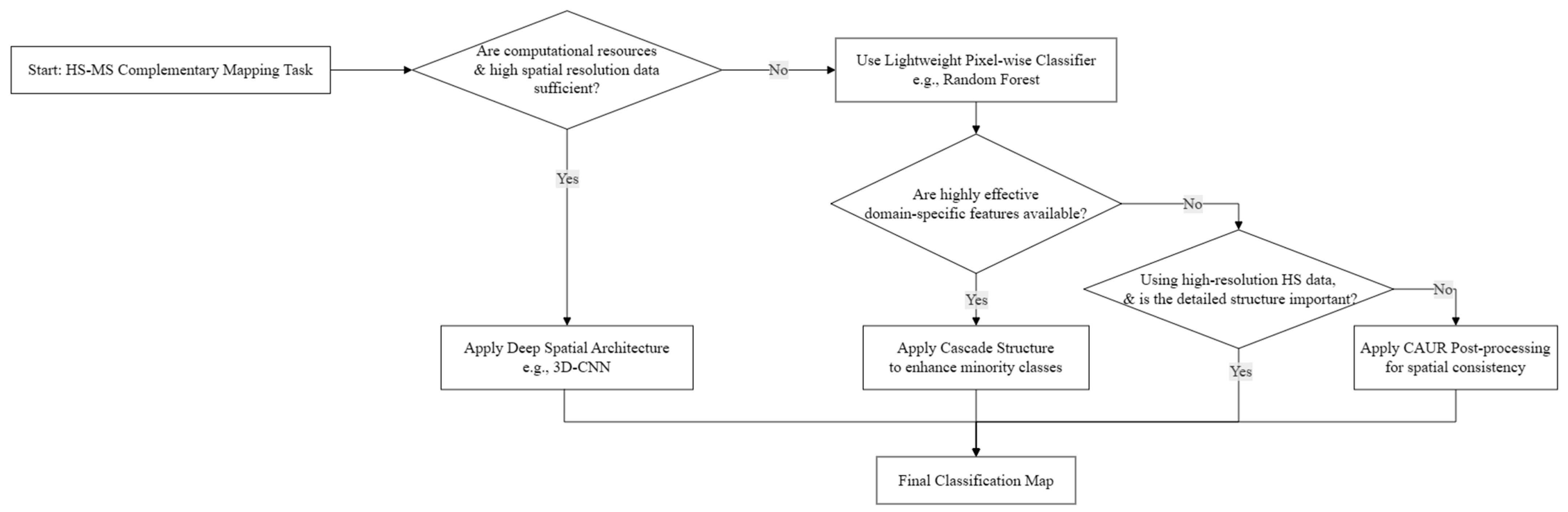

Disclaimer/Publisher’s Note: The statements, opinions and data contained in all publications are solely those of the individual author(s) and contributor(s) and not of MDPI and/or the editor(s). MDPI and/or the editor(s) disclaim responsibility for any injury to people or property resulting from any ideas, methods, instructions or products referred to in the content. |
© 2026 by the authors. Licensee MDPI, Basel, Switzerland. This article is an open access article distributed under the terms and conditions of the Creative Commons Attribution (CC BY) license.