


Abstract
Transformer layers can develop distinct attention routing patterns during training, but how architectural access to structural information shapes this organization remains unclear. Existing structure-aware methods make this difficult to determine by modifying several components. To investigate this question, we compare two Transformers matched in field ID inputs, embeddings, learned components, backbone, parameter count, and optimization but differing in attention computation. Both use field embeddings; Structure-Aware Attention Bias (SAAB) additionally transforms the supplied field IDs into a fixed pairwise same-field attention bias. We first train both models on the DBpedia dataset with masked structure modeling (MSM), which requires the recovery of hidden field labels from the context. Both models exceed 99.9% validation accuracy, yet they organize attention differently. Across 64 paired validation examples from the seed-1001 model pair, SAAB changes the mean same-field attention mass (SFM) by −0.085 at Layer 2 and +0.048 at Layer 3 (95% confidence intervals: [−0.092,−0.078] and [+0.042,+0.055]). We call this pattern competitive displacement. Across eight initializations, two show relatively strong displacement; the others show weaker or different responses. For seed 1001, displacement varies non-monotonically with the bias strength. Related changes persist with depth in two selected seeds and appear differently on PubMed. These results show that SAAB redistributes layer-wise attention routing under tested conditions.
1. Introduction
Transformer layers develop different representation and attention routing patterns during training. This organization is not built into the design, which means that the layers begin without predefined routing patterns and their distinct patterns develop during training [1,2,3,4,5]. Previous studies have shown that even minor architectural modifications can alter how information is distributed across the network’s layers [6]. However, it remains unclear how specific architectural choices independently contribute to these shifts when other architectural and training factors are controlled. Recently, several studies have investigated how training dynamics, such as the training time, influence the emergence of different internal representations during training [7,8]. While these studies offer valuable insights into representation dynamics, they attribute such shifts to training-related factors, such as the training time. It remains unclear whether a controlled change in how existing structural information is made accessible to attention, without changing the training procedure, can trigger a comparable shift in layer-wise attention routing. The closest approaches incorporate structural relations into their attention mechanisms [9,10,11], but these approaches commonly also change the input representations, learned components, or attention operations. Consequently, any observed changes in attention routing may result from several changes rather than from any one intervention. In this work, we investigate whether an additional fixed pairwise structural pathway in attention can change layer-wise routing. To examine this intervention, we conduct a controlled study in which the field ID inputs, learned components, Transformer backbone, model capacity, downstream task, and optimization process are held constant, while SAAB additionally supplies a fixed pairwise same-field relation to the attention logits. This experimental design tests the combined effects of the additional pathway, pairwise relation, and attention-level access without attributing the result to the injection location alone.
Structural deep learning methods make information accessible through several learning paradigms. Supervised task-specific systems organize features for labeled prediction while incorporating structure through segmentation, graph interaction, or constrained attention, as illustrated by TableStructureFormer and Doc2GraphFormer [12,13]. Self-supervised and mixed-objective models instead learn structural representations through masking or reconstruction objectives, including LayoutLMv3, UDOP, and DocLLM [14,15,16]. Unsupervised and domain-adaptive methods can organize unlabeled target-domain features through cross-domain alignment and graph interaction [17]. Structural prior and graph-driven methods make relations directly available through typed graph neighborhoods or attention constraints [9,10,11]. These paradigms differ in how information interacts, whether the structure is learned or supplied, and whether features are organized for prediction, reconstruction, domain alignment, or relational processing. This comparison motivates the examination of structural information from the perspective of architectural accessibility.
Our key idea is to use structured data to create a controlled additional pathway in the network. To this end, we propose Structure-Aware Attention Bias (SAAB) and compare it with a conventional Transformer baseline. Both models use the supplied field IDs through the same field embedding pathway. SAAB additionally converts these IDs into an explicit pairwise same-field relation and adds the resulting fixed, nontrainable bias to the attention logits in every layer. It therefore introduces neither a new field label source nor additional trainable parameters, although it changes the attention computation. The baseline and SAAB share the same Transformer backbone, embeddings, learned components, prediction head, and trainable parameter count, but differ in attention computation. Their comparison provides a controlled evaluation of the tested fixed pairwise attention pathway and its effects on layer-wise attention routing. As illustrated in Figure 1, the baseline can represent field relationships through the field information already present in its hidden representations, whereas SAAB makes an explicit same-field relation directly accessible in attention.
Figure 1.
Baseline and SAAB architectures. (A) The variants share the same input representation, embeddings, Transformer backbone, and MSM prediction head. (B) They differ in self-attention computation: the baseline uses standard self-attention, whereas SAAB additionally adds the nontrainable pairwise bias to the attention logits.
We train both models using masked structure modeling (MSM), a self-supervised task derived from masked language modeling (MLM) [18]. In MSM, a subset of field tags is masked while all textual content remains visible; the model recovers the missing tags from token content and the remaining visible structural context. Consequently, MSM provides a controlled task in which the field structure is directly relevant to prediction. Our experiments are primarily conducted on the DBpedia dataset [19,20], a large-scale collection of Wikipedia articles in which each instance consists of two field tags, including a short title and a longer body description. We intentionally use only two field tags to construct a controlled and simplified setting where every attention interaction can be clearly identified as occurring either within the same field or across different fields, enabling an unambiguous analysis of the measured results. To examine the routing response in a different domain and a more complex field structure, we conduct additional experiments on the PubMed 200k RCT dataset [21], where each instance contains three distinct fields. Across these experiments, we find that the additional fixed pairwise pathway can influence how within-field and cross-field attention are distributed across Transformer layers. Although the two models achieve comparable task performance in terms of accuracy and loss, they develop different layer-wise routing organizations. In the two relatively strong displacement cases, one layer shifts toward more cross-field routing, while another shifts toward more within-field routing relative to the baseline. We term this phenomenon competitive displacement and study it in detail in this work. Beyond this specific pattern, the study identifies the direct attention-level accessibility of the fixed pairwise field relation as an architectural factor that can change routing organization without changing task performance. For explainable AI, this controlled comparison helps to show that comparable predictive performance can coexist with different measured attention routing organizations. The main contributions of this paper are as follows:
- We show that adding a fixed pairwise field relation directly to attention can reshape layer-wise attention routing, even when the models receive matched field ID inputs, have the same trainable parameter count, and achieve comparable task performance.
- We introduce SAAB, which reuses the supplied field IDs through an additional fixed pairwise pathway in attention, enabling a controlled comparison in which the tested pathway differs while the shared components and training protocol remain fixed.
- Using controlled experiments and MSM loss gradient analysis, we characterize a routing reorganization pattern called competitive displacement and report its associated changes in layer-wise routing and gradient strength.
- Through a systematic evaluation across five tested bias strengths and eight random initializations, we show that competitive displacement varies non-monotonically with the bias strength at seed 1001 and that relatively strong displacement occurs in two of the eight initializations.
- We evaluate the effect in deeper Transformer models and on a second dataset, showing that routing reorganization persists in two selected deeper-model runs and takes a distinct form on PubMed, while the affected layers vary with the model depth, initialization, and dataset.
The remainder of this paper is organized as follows. Section 2 reviews supervised, self-supervised, unsupervised, and structural prior approaches together with analytical work on layer-wise attention routing and training dynamics. Section 3 describes our proposed SAAB model, the baseline model, and the MSM task. Section 4 gives the datasets and training details. Section 5 presents the experimental results in three parts: the observed layer-wise reorganization and its development during training, controlled experiments that identify the conditions under which it occurs, and an evaluation of its variation across random initializations, its conditional persistence across network depths, and its appearance in a second dataset. Section 6 discusses the implications of our findings and their limitations, while Section 7 summarizes the main contributions and concludes the paper.
The reference implementation, experimental configurations, and analysis scripts are publicly available at https://github.com/mira-bau/layer-routing (accessed on 28 July 2026).
2. Related Work
Understanding how structural information shapes attention routing requires consideration of both how the structure is learned and how it becomes architecturally available within a model. With respect to learning paradigms, prior work spans supervised task-specific methods, self-supervised or mixed-objective pretraining, and unsupervised or domain-adaptive learning. From an architectural perspective, we categorize prior work into structural prior and graph-driven methods, which incorporate relational information through input representations, graph construction, or attention mechanisms. These approaches differ in how information interacts, how the structure is modeled, and how learned features are organized. We first review these four areas and then turn to Mixture of Experts routing and complementary studies of layer-wise organization and training dynamics.
2.1. Supervised Task-Specific Structural Modeling
Supervised models for document, table, and structured data tasks encode rows, columns, page positions, field identities, or graph relations while optimizing labeled prediction objectives. Existing approaches incorporate this information through dedicated input embeddings, constrained attention, or graph interaction [10,11,22,23,24]. TableStructureFormer, for example, combines supervised row–column segmentation with masked attention, while Doc2GraphFormer combines graph message passing with global self-attention for document understanding [12,13]. Transformer models for structured and tabular data also learn embeddings for field identity, temporal information, or other structural attributes [25,26,27,28]. These methods organize structural features for downstream prediction through different combinations of structural inputs, task heads, attention constraints, and message passing components.
2.2. Self-Supervised and Mixed-Objective Structural Pretraining
Unlike supervised task-specific systems, self-supervised and mixed-objective document models learn structural representations through masking or reconstruction, sometimes together with labeled tasks. LayoutLMv3 jointly masks text and image content, UDOP combines self-supervised reconstruction with supervised objectives, LayoutMask predicts masked tokens and two-dimensional positions, and DocLLM uses segment infilling with disentangled text and spatial attention [14,15,16,29]. These methods organize features around reconstruction or pretraining objectives. MSM follows this general paradigm by learning to recover masked field labels from the context.
2.3. Unsupervised and Domain-Adaptive Structural Learning
Whereas self-supervised pretraining organizes features through masking or reconstruction objectives, unsupervised and domain-adaptive methods organize target-domain features without target labels, often by combining cross-domain alignment objectives with graph-based interaction. Graph Harmony combines nuclear-norm Wasserstein alignment with a variational graph autoencoder to address shifts in structural patterns across domains [30]. Wang et al. construct multi-domain prototypes and use graph interaction to align category-level representations for unsupervised rotating machinery fault diagnosis [17]. Both approaches use structural interaction to organize features across source and target domains. They illustrate how structure can support domain-invariant feature organization—a different use of structure compared to the architectural accessibility question considered here.
2.4. Explicit Structural Priors and Attention Modification
Across these learning paradigms, a separate architectural question concerns how structural relations are made available through attention design, input encoding, or graph construction. Transformer approaches incorporate structural information for graph, relational, tabular, and web data through typed or relation-aware attention, learned attention biases, attention masks, input positional encodings, and structural encoders [9,10,11,31,32,33,34,35]. Other work characterizes relational inductive biases in attention mechanisms [36]. Some approaches use fixed graph-derived attention patterns [37], explicitly separate relational from object-level features [38], or analyze how relational inductive biases vary across learning settings [39]. Graph neural networks instead encode relational priors through message passing over explicit edges and can represent richer, domain-defined topologies [40]. These methods supply structure through explicit edges, fixed attention patterns, learned structural biases, or relation-aware representations. Attention regularization and sparse attention methods impose different constraints. Scheduled DropHead stochastically removes entire attention heads during training [41]. Selective self-attention uses query-dependent temperature scaling to control attention concentration, whereas native sparse attention changes attention support for efficient long-context processing [42,43]. SAAB provides a contrasting constraint: it preserves all attention heads and dense token-to-token attention while adding a fixed structural relation to the attention scores. Taken together, these methods constrain attention at different levels, including head availability, attention concentration, attention support, and pairwise structural scoring. They can therefore influence within-layer attention organization through different mechanisms.
2.5. Mixture of Experts Routing
Beyond attention and graph constraints, Mixture of Experts models provide another form of computational organization. They use learned dynamic routers to assign tokens to distinct parameterized experts, with router design affecting expert utilization, load balance, and specialization [44,45]. By contrast, SAAB changes attention routing within Transformer layers rather than routing tokens among parameterized experts. MoE expert specialization and layer-wise attention routing are therefore related organizational concepts but not interchangeable mechanisms.
2.6. Layer-Wise Organization and Training Dynamics
Whereas MoE models organize computation across explicitly parameterized experts, a complementary body of literature examines how representations and attention patterns become distributed across depth within a Transformer. Early studies of BERT used lightweight classifiers on internal representations to show that grammatical and semantic information is distributed differently across layers [1,2]. Individual attention heads have also been associated with grammatical dependencies or coreference relations [3]. These studies establish that representations and attention patterns vary across depth, while changes to pretraining objectives or model architecture can alter this distribution [6]. Related work examines component-level organization and its emergence during training [46,47,48]. Causal intervention and mechanistic interpretability work further traces the contributions of components and circuits [4,49,50]. Induction heads, for example, can emerge through a relatively sharp transition during training [5]. More broadly, grokking and theoretical studies show that learning dynamics can change abruptly as the training conditions, data scale, or initialization vary [7,8,51,52]. Together, this literature shows that component-level organization can emerge over training and vary with the training conditions and data scale. Optimization dynamics provide one possible explanation for differences across depth because the loss signal can be distributed unevenly across layers [53]. Repeated training can also produce different internal solutions across initializations despite comparable task performance [54,55,56,57]. Together, these findings connect depth-wise organization with optimization dynamics and initialization variability.
Taken together, prior methods demonstrate that structural information can shape representations and attention, but they often change the inputs, objectives, trainable components, or relational mechanisms together. This leaves it unclear how attention organization responds when structural accessibility changes under otherwise matched conditions. To address this gap, we use a controlled baseline–SAAB comparison, defined in the following section.
3. Proposed Models and Methodology
We examine how adding a fixed pairwise structural pathway to attention influences layer-wise attention routing by comparing SAAB with a conventional Transformer baseline. The two variants receive the same token and field ID inputs and share the same embeddings, encoder dimensions, Transformer backbone, prediction head, learned components, and trainable parameter count. They differ in attention computation: SAAB retains the field embedding pathway and additionally converts the field ID tensor supplied to the model into a nontrainable pairwise relation in the attention logits. This controlled comparison evaluates how the additional attention-level pathway affects layer-wise routing under the reported controls. In the remainder of this section, we first describe the shared Transformer architecture and then present the baseline and SAAB models, and we finally introduce the masked structure modeling task used for evaluation.
3.1. Shared Components and Parameterization
As illustrated in Figure 1, the baseline and SAAB models share the same Transformer backbone, embeddings, learned components, prediction head, and trainable parameter count, but differ in attention computation. The shared encoder takes structured input data and converts them into a single ordered sequence of tokens, where each token is associated with a field ID indicating the field from which it originates. At position i, is the token ID and is the field ID supplied to the model; during MSM, is the field ID after masking. The implemented embedding computation is
Consequently, the field ID is embedded in the hidden representation from the first layer in both models. The resulting sequence is then processed by a pre-layer-normalized Transformer encoder with four layers, a model width , six attention heads, a feedforward network with 3072 hidden units in each layer, a dropout rate of 0.2, and layer normalization with . The feedforward sublayers use GELU activations, and the encoder uses residual connections and a final layer normalization. A shared linear token-level head maps the final hidden states to field ID logits. The baseline and SAAB therefore have matched parameterization but different attention computations. An equal trainable parameter count does not imply equal runtime or memory costs; these quantities are evaluated separately in the computational overhead analysis.
3.2. Baseline Model
The shared Transformer architecture shown in Figure 1 serves as the baseline model. Field embeddings influence the hidden states and therefore the queries and keys, but no fixed same-field indicator is added directly to the attention logits. The attention computation follows the standard formulation introduced in [58], where the softmax operation converts the pairwise attention scores into normalized weights that are nonnegative and sum to one. Both variants apply the ordinary key padding mask before the softmax. The baseline can learn field-level relations through the field information already present in its hidden representations.
3.3. SAAB: Structure-Aware Attention Bias
As illustrated in Figure 1, the proposed SAAB model uses the same shared Transformer encoder as the baseline model. However, unlike the baseline, SAAB introduces an additional information pathway. In addition to incorporating field IDs into the input embeddings, SAAB adds to the scaled attention scores:
Here, is the per-head key dimension.
For an input sequence of length n, SAAB constructs from the field ID tensor g supplied to the model:
where i and j index token positions and equals one when its condition is true and zero otherwise. Equal supplied field IDs receive an additive bias of , whereas unequal IDs receive zero. Because the bias is applied before the softmax, multiplies a pair’s unnormalized attention weight by e, holding the learned attention logits fixed; it does not add 1 to the final attention probability. During MSM, g is the already masked field ID tensor. Thus, two selected positions match through the shared [FIELD_MASK] ID, while an original target identity never enters the indicator relation. The ordinary key padding mask remains active independently, so padded keys do not contribute to attention. The matrix is broadcast across all heads and, in the main SAAB model, is added in every encoder layer.
The structural bias depends only on the supplied field IDs and remains independent of token content. This additional pathway introduces no additional trainable parameters. The bias is input-dependent but nontrainable: its construction rule and are fixed in the main comparisons, while the dedicated bias strength ablation varies explicitly. The matrix is recomputed from each input’s field ID tensor, and the same masked tensor supplies both the field embeddings and . Keeping this rule fixed preserves the shared learned components and trainable parameter count while changing the explicit pairwise relation available to attention. The paired comparison therefore tests the routing response to this combined intervention; it does not isolate a causal effect of the injection location alone.
3.4. Masked Structure Modeling (MSM)
MSM is a self-supervised task in which the model reconstructs masked field labels from the context. It is inspired by masked language modeling [18], but, instead of predicting masked tokens, it focuses on predicting structural tags. The text tokens remain unchanged, so prediction can use the token content together with the unmasked structural context.
Masking is performed across each micro-batch and separately for every field ID represented at non-padding positions. Let be the eligible positions and the positions carrying field ID f. For every nonempty , the seeded generator samples without replacement positions. Thus, each represented field contributes approximately 15% of its eligible positions, with at least one selected position. Padding is excluded, and the masking routine applies no additional field ID filtering.
Before the forward pass, the selected entries of F are copied only into the prediction-target tensor and are then replaced with the shared [FIELD_MASK] ID to form . The token sequence X is unchanged. Both variants receive and use for their field embeddings; SAAB also constructs from . The original field IDs are never passed to either model at the selected positions.
Keeping the input text visible is essential to the design of MSM. In conventional downstream tasks, such as document classification, models may achieve high performance by exploiting semantic content without necessarily learning to organize attention according to the document structure. Consequently, task performance alone provides limited insight into whether structural routing has emerged. MSM instead supplies a common field label recovery objective and known field boundaries for comparing the paired models’ attention routing. Because the field identity remains recoverable from the token content and unmasked structural context, MSM does not assign successful prediction to a single route, and a particular SFM value is neither necessary nor sufficient for solving the task. Both variants receive the same tokens, masked field ID tensor, targets, and training procedure; the comparison tests whether SAAB’s additional fixed pairwise pathway changes the measured routing organization while the models solve the same task. Figure 2 illustrates the MSM design, and Algorithm 1 details the training procedure.
| Algorithm 1: Masked Structure Modeling for Baseline and SAAB |
Input: token IDs X, original field IDs F, attention mask A, variant , masking rate , accumulation count R, shared [FIELD_MASK] ID m, and seeded masking generator G. Optional control (SAAB-shuffled): shuffled bias flag c and shuffle seed s. Output: trained parameters and optional gradient summaries. for each optimizer step t do Set the scheduled learning rate and clear accumulated gradients. for micro-batch do ; . for each field f represented in E do ; set . Sample , , without replacement using G; set . end for Y ← IGNORE_INDEX and ; set and . if then set . else set . If c is enabled, permute only among positions where using s; retain unpermuted for the embeddings. Set with and add B in every encoder layer. end if Forward only and obtain token-level logits Z. ; backpropagate . end for If gradient diagnostics are enabled, record each layer’s joint Q/K/V weight gradient norm after accumulation and before clipping. Clip the global gradient norm, apply the AdamW update, and advance to the next optimizer step. end for |
Figure 2.
Design of masked structure modeling (MSM) task. Selected field IDs are replaced with the shared [FIELD_MASK] ID before the forward pass, while the token text remains unchanged. Both variants embed the masked IDs, and SAAB also derives its fixed pairwise bias from them. Original field IDs are used only as prediction targets.
4. Experimental Setup
This section presents the experimental setup used throughout the study. We describe the datasets, training configuration, and implementation details, followed by the evaluation protocol and the measurements used to compare the baseline and SAAB models.
4.1. Datasets and Evaluation
Our primary experiments based on MSM are conducted on the DBpedia dataset [19] using the simplified two-field setting, where each document consists of a short title and a longer content description. We intentionally restrict the input to two field IDs to create a controlled setting in which every attention interaction can be clearly classified as occurring either within the same field or across different fields, enabling a clear interpretation of the resulting measurements. Each document is converted into a single sequence of tokens, with every token assigned a field ID indicating its source field. The original DBpedia training split contains 560,000 examples. We divide it into 490,000 training examples and 70,000 validation examples using a deterministic random split with seed 42. The benchmark’s original test split is excluded from training, validation, and checkpoint selection and is used only for the confirmatory analysis reported in Section 5.10. The models are trained for 500 optimization steps. Unless otherwise specified, the detailed routing and bias strength analyses use seed 1001. The gradient analysis uses seed 1001 as the main case and is repeated for seed 99, which also shows relatively strong displacement, and seed 42, which does not. Training loss curves are reported as the average over three independent runs with random seeds 42, 123, 1001, while a more comprehensive evaluation across eight random initialization seeds is presented in Section 5.4.
To track the development of routing behavior during training, we record model checkpoints at optimization steps 1, 10, 50, 100, 200, 300, and 500. At each checkpoint, we evaluate attention patterns using the first 32 examples from the validation split. We repeat the analysis using the first 64 validation examples to confirm that the observed patterns are not sensitive to the number of examples used. The maximum absolute difference between the corresponding layer-wise SFM values is less than 0.005, which is small relative to the strong L2 decreases of 0.085 and 0.469 observed at seeds 1001 and 99. We analyze the final routing behavior at step 500 because both models reach comparable loss and accuracy levels at this point. The routing differences are therefore observed despite the comparable final task performance; the trajectory analyses below examine how their development coincides with the measured optimization signal.
To examine routing effects in a different domain and a more complex field structure, we replicate our analysis on PubMed 200k RCT [21], a biomedical abstract dataset derived from randomized controlled trial reports. In this experiment, we use the provided training and development splits and retain only abstracts containing all three structural fields (i.e., methods, results, and conclusions), resulting in 177,533 training records and 2336 validation records, with mean sequence lengths after tokenization and the configured 512-token cap of 293.400 tokens in training and 295.100 tokens in validation. Each retained record is linearized in the fixed order of methods, results, and conclusions, and the MSM task is extended from binary field prediction to a three-field prediction problem. Models are trained for 1500 optimization steps using three random seeds 42, 123, 1001, and the primary routing comparison uses the first 64 validation examples at a 256-token evaluation cap; Section 5.11 reports the corresponding 512-token reevaluation.
4.2. Training Protocol
Both models are trained under identical experimental settings. Within every reported seed pair, both variants start from the same initial parameter tensors and use the same prepared-example order, batching, MSM mask generator state, and optimization configuration. Retained run artifacts confirm matching sample-row and sample-batch hashes and identical trainable parameter counts within each pair. The variant setting determines whether the fixed SAAB attention bias path is active. This pairing controls the within-seed comparison but does not imply bitwise-identical execution across different software or hardware environments. The implementations use PyTorch 2.11.0 with CUDA 12.8, and tokenization is performed using the Hugging Face tokenizers library (version 0.22.2). The Transformer, SAAB, MSM, training, and evaluation implementations use custom PyTorch code; Hugging Face Transformers is not used. The recorded run environments additionally use Python 3.12.13, NumPy 2.0.2, pandas 2.2.2, PyYAML 6.0.3, and scikit-learn 1.6.1. We optimize the models with AdamW using a learning rate of , weight decay of , and momentum parameters . Gradients are clipped to a maximum global norm of 1.0. Training uses a micro-batch size of 64 with gradient accumulation over eight steps, giving an effective batch size of 512 examples. The MSM loss is divided by eight before each backward pass. When joint Q/K/V gradient norms are analyzed, they are measured after all eight gradients have accumulated and immediately before global clipping. The learning rate is linearly warmed up during the first 50 optimization steps and subsequently decayed using a cosine schedule to 10% of its peak value. Input sequences are truncated to 256 tokens for the DBpedia dataset and 512 tokens for PubMed. Training and evaluation use the standard float32 tensor path without automatic mixed precision or gradient scaling. No explicit TF32 override was applied, and both variants within each pair used the same numerical configuration. Python, NumPy, PyTorch, CUDA, data loader, and MSM masking generators are explicitly seeded. Each run used one NVIDIA A100-SXM4 GPU, (NVIDIA Corporation, Santa Clara, CA, USA) with 40 GB of VRAM, provided through Google Colab.
4.3. Metrics and Analyses
The primary objective of this study is to characterize layer-wise attention routing rather than to optimize task performance. Task accuracy and loss are therefore treated as secondary measures. Comparable values indicate that the observed routing differences are not accompanied by a gross failure in predictive performance, but they do not eliminate possible differences in training dynamics. To quantify layer-wise attention routing, we introduce the same-field mass (SFM) metric. Inside each layer, each valid named-field query allocates attention to tokens in the same field and to tokens in other fields. The SFM summarizes this allocation; it does not measure a layer’s complete computational function.
The SFM is defined within each example as the mean, across heads and valid named-field query positions, of the attention probability assigned to valid named-field keys with the same field ID; the resulting values are then averaged equally across examples. Positions are valid only when they are non-padding and belong to a named analysis field; attention to other keys is not reassigned before the same-field mass is summed. An SFM value of 1.0 indicates that a layer attends exclusively within fields. In addition to the SFM, we report the attention entropy to characterize the concentration of attention distributions, indicating whether a layer distributes attention broadly across tokens or concentrates it on a smaller subset. Entropy is computed with the natural logarithm and reported in nats. It is averaged within each example over heads and the same valid query positions and then equally across examples. It uses the model’s unmodified attention distribution and is not renormalized to the named-field keys. When we describe a layer as the cross-field layer, or say that it shifts toward cross-field routing, we mean its routing pattern relative to the other layers. In the standard four-layer DBpedia comparison, we use competitive displacement to describe the relatively strong paired reorganization in which SAAB decreases the L2 SFM and increases the L3 SFM relative to the corresponding baseline layers, enlarging the L3−L2 SFM gap. Because the effect magnitudes vary across initializations, Section 5.4 reports the seed-wise layer changes directly. “Competitive” names the observed redistribution; it does not assert literal optimization competition between layers.
The raw SFM has an example-specific neutral level because fields can contain different numbers of valid tokens. For example e, let be the number of valid tokens in field f, and let . We define the same-field opportunity and opportunity-adjusted SFM as
Equivalently, counts the available ordered same-field query–key pairs among the valid named-field pairs, making the same-field mass expected under uniform attention. For both raw and adjusted analyses, a valid position must be non-padding and carry one of the named analysis field IDs (title/content for DBpedia; methods/results/conclusions for PubMed). Padding, special or unknown field IDs, and the MSM mask field ID are not included in or . The adjusted SFM is zero at this neutral reference, one when attention is exclusively within fields, and negative when attention allocates more mass across fields than the neutral opportunity. It is undefined when only one named field is visible; such examples are retained in the raw SFM analyses but counted and excluded from the adjusted summaries.
To examine how the optimization signal is distributed across layers, we record the gradients of the actual MSM cross-entropy loss on the masked training batches at every optimization step. After accumulating gradients over eight micro-batches and before global gradient clipping, we calculate the joint L2 norm of the Q, K, and V projection weight gradients in each attention layer. We then compare L3 and L2 using the ratio of their norms. A ratio above 1.0 indicates a larger loss gradient magnitude at L3, while a ratio below 1.0 indicates a larger magnitude at L2. Because individual training batches introduce variation, we summarize this ratio using a trailing mean over up to 10 optimization steps and report it at selected checkpoints. This measure describes the relative gradient strength; it does not provide the gradient direction, show whether the SFM will increase or decrease, or represent the parameter update magnitude produced by AdamW. To summarize differences in layer-wise routing with a single quantitative measure, we define the profile distance as the Euclidean distance between the layer-wise SFM vectors of the two models . This metric quantifies the overall difference in routing organization across the Transformer encoder.
5. Experiments and Results
We first establish the principal routing difference between the baseline and SAAB models and trace its emergence alongside the measured loss gradient signal (Section 5.1, Section 5.2 and Section 5.3). We then characterize its variation across initializations and probe the roles of the bias strength, layer placement, and alignment with field structure (Section 5.4, Section 5.5, Section 5.6 and Section 5.7). Finally, we examine deeper DBpedia models and PubMed, quantify paired uncertainty and field opportunities, confirm the principal pattern on untouched test records, assess sequence length effects, and report the computational overhead (Section 5.8, Section 5.9, Section 5.10, Section 5.11 and Section 5.12).
5.1. Effects of the Fixed Pairwise Structural Path on Layer-Wise Attention Routing
To determine whether the fixed pairwise structural path is associated with different layer-wise routing, we compare the baseline and SAAB models at optimization step 500, when both models have reached comparable performance on the DBpedia dataset: validation accuracy of 0.9997 and training loss of 0.0021. Table 1 reports the results based on the selected evaluation metrics of the SFM and attention entropy (defined in Section 4.3) for the four layers spanning the first layer (L0) to the last layer (L3).
Table 1.
Task performance and layer-wise routing at optimization step 500 for seed 1001. SFM and attention entropy are computed over 64 held-out validation examples. Bold values indicate the highest SFM within each model.
Table 1 shows that the two models develop different routing patterns across their layers, with the clearest change occurring at L2 and L3. Compared with the baseline, SAAB decreases the SFM by 0.084 at L2 and increases it by 0.050 at L3, moving the highest SFM from L2 to L3. Across all four layers, the increases and decreases balance each other, leaving the average SFM nearly unchanged (0.859 in the baseline and 0.861 in SAAB) and showing that SAAB redistributes within-field routing across layers rather than increasing it uniformly. Paired confidence intervals, effect sizes, and Holm-adjusted permutation test p-values for these layer-wise changes are reported in Table 2. We refer to this shift from L2 to L3 as competitive displacement because L3 becomes the strongest within-field layer while L2 moves in the opposite direction by attending more to tokens in the other field. At L2, cross-field attention nearly doubles, from 9.6% in the baseline to 18.0% in SAAB, while most of its attention still remains within fields, meaning that its routing role changes relative to the baseline without completely reversing. The change at L2 is also reflected in its attention entropy, which decreases from 3.80 in the baseline to 3.55 in SAAB—the lowest value reported in Table 1. This decrease shows that L2’s attention becomes more concentrated overall, even as a larger share is dispersed across fields.
Table 2.
Paired per-example DBpedia SFM changes for the fixed seed-1001 model pair on the same 64 held-out validation examples. is SAAB minus baseline, CI is the paired-bootstrap 95% confidence interval, is the paired Cohen’s effect size, and is the Holm-adjusted paired permutation test p-value.
To quantify uncertainty across records for this fixed model pair, we reproduced the DBpedia comparison on the same 64 held-out validation examples and calculated the paired per-example difference—SAAB minus baseline. The reproduced mean SFM values were within 0.004 of those in Table 1. For each layer, we estimated a 95% confidence interval via paired bootstrap resampling and applied a two-sided paired sign-flip permutation test, with Holm correction across the four layers. Table 2 reports the results.
The confidence intervals exclude zero at all four layers, supporting increases at L0 and L3 and decreases at L1 and L2 for this fixed model pair. These tests quantify the variability across validation examples conditional on the fixed seed-1001 pair; they do not measure variability across independent training initializations, which is examined separately in Section 5.4. Each interval uses 10,000 paired-bootstrap resamples, and each two-sided sign-flip test uses 20,000 draws. With the plus-one permutation correction, the minimum attainable raw p-value is ; the corresponding Holm-adjusted value across the four layers is .
Figure 3 shows which field-to-field interactions contribute to the redistribution between L2 and L3. In each matrix, rows show where attention originates and columns show where it is directed. Thus, the bottom-left cell represents attention from content tokens to title tokens, while the top-left cell represents attention from title tokens to other title tokens. Compared with the baseline model, SAAB increases content-to-title attention at L2 by more than three times, from 4.7% to 14.9%. This means that more attention from content tokens crosses into the title field, contributing to the lower SFM at this layer. At L3, the change is toward stronger within-field routing, with title-to-title attention increasing by 16.5 percentage points, from 49.3% in the baseline to 65.8% in SAAB. Together, these field-level changes show that SAAB shifts the attention routing of L2 and L3 in opposite directions rather than increasing within-field attention uniformly across layers.
Figure 3.
Field-to-field attention at L2 and L3 for the baseline and SAAB models at step 500 for seed 1001. Attention values are computed over 64 held-out validation examples. Rows indicate source fields, and columns indicate attended fields.
Figure 4 complements the field-level averages with one word-level example from the untouched DBpedia test split. Without inspecting model outputs, we selected the lowest-index record satisfying the predeclared length and field coverage criteria within the deterministic 2,336-record sample. Its title is Aerostar, and its content is Aerostar S.A. is an aeronautical manufacturing company based in Bacău Romania. Attention is averaged over all six heads. To obtain readable words, BPE query-piece rows are averaged, and attention to the key pieces of each word is summed. Title start and content start denote the special tokens inserted before the respective fields. In Figure 4, T and C distinguish the title and content occurrences of Aerostar, and the horizontal and vertical lines separate title tokens from content tokens.
Figure 4.
Word-level attention at L2 and L3 for the baseline and SAAB models on one DBpedia test record at step 500 for seed 1001. Rows indicate query words or field-start tokens, columns indicate attended words or field-start tokens, and all panels use the same attention weight scale.
The four maps show that SAAB reorganizes this record differently across depth rather than uniformly increasing same-field attention. At L2, SAAB produces a stronger vertical band at the title occurrence of Aerostar: most content words redirect more attention toward the title field. For example, attention from manufacturing to the title occurrence increases from to , and attention from company increases from to . The change is selective rather than uniform; attention from content start to the same title word decreases from to . At L3, the organization shifts toward clearer field separation. The title occurrence’s attention to itself increases from to , while attention from content start to this title word decreases from to , and most content queries reduce their total attention to title keys. Thus, this record illustrates one way in which greater content-to-title routing at L2 and stronger title-field consolidation at L3 can produce opposing aggregate SFM directions. Because it represents one record and one fixed model pair, the figure is a qualitative illustration rather than inferential or across-seed evidence.
5.2. Tracing Layer-Wise Routing Differences in SAAB and Baseline
To examine how routing patterns develop during training, we track the SFM across all four layers at selected checkpoints for the baseline and SAAB models trained with seed 1001. Since competitive displacement in this four-layer model occurs between L2 and L3, we use their trajectories to determine when the pattern emerges. Figure 5 traces the SFM across all four layers for seed 1001.
Figure 5.
Same-field mass (SFM) per layer across training for seed 1001. Each marker is the mean SFM over 32 fixed held-out validation examples; lines connect recorded checkpoints without smoothing. The L3−L2 separation is temporary in the baseline and persists in SAAB.
At the first recorded checkpoint, step 1, the SFM is nearly uniform across the layers within each model, with values of around 0.83 in the baseline and 0.90 in SAAB. SAAB begins at a higher level because the fixed bias favors same-field attention from the start of training, but no individual layer stands out in either model. By step 50, the mean training loss has fallen sharply in both models, while their layer-wise routing profiles remain nearly flat, showing that the early reduction in loss occurs before a clear difference develops between L2 and L3. The difference becomes visible between steps 100 and 200. In the baseline, L3 overtakes L2 at step 200, but this change is temporary because L2 again has the highest SFM at step 500. In SAAB, L3 continues to increase while L2 decreases, producing an L3−L2 gap of 0.109 at step 200 and 0.129 at step 500. The same temporary rise for L3 therefore appears in the baseline, but SAAB develops a much larger and persistent separation between the two layers. The competitive displacement pattern therefore develops after the early reduction in loss rather than being present at the first checkpoints.
5.3. Layer-Wise Gradient Differences Accompanying Routing Reorganization
Table 1 shows that the clearest competitive displacement pattern occurs between L2 and L3, even though SAAB applies the same fixed bias to both layers. Because uniform bias placement does not by itself explain the unequal measured response, we examine whether the routing separation is accompanied by a difference in the MSM loss gradient magnitude received by the two layers during training. Figure 6 reports this comparison for seed 1001 using the ratio of the L3 gradient norm to the L2 gradient norm at selected checkpoints. A ratio above 1 indicates a larger gradient at L3, whereas a ratio below 1 indicates a larger gradient at L2. Each point represents a trailing mean over up to 10 training steps.
Figure 6.
L3-to-L2 MSM loss gradient norm ratio for seed 1001 (log scale). Points show trailing means over up to 10 steps at selected checkpoints.
At the early checkpoints, the two models have almost identical gradient ratios, with 10-step means of 1.027 in the baseline and 1.028 in SAAB at step 50. After step 50, the ratios move in opposite directions: by step 100, the baseline ratio rises to 1.374, while the SAAB ratio falls to 0.312, and, by step 200, the corresponding values are 2.841 and 0.161. This means that the baseline develops a larger MSM loss gradient magnitude at L3, whereas SAAB develops a larger magnitude at L2. The individual SAAB norms show the size of this difference: averaged over steps 191–200, the L2 gradient norm is 0.00544 and the L3 norm is 0.00086, making the L2 gradient approximately 6.3 times larger.
The timing of this gradient separation is important because the ratios have already diverged by step 100, while the SAAB L3−L2 SFM gap remains only 0.025, compared with 0.001 at step 50 and 0.109 at step 200. The relative gradient strengths therefore begin to separate before the L2–L3 routing separation becomes large, and they remain different as the routing patterns diverge. However, gradient norms measure only magnitude and not direction, so these measurements show how the gradient and routing differences develop over time but do not prove that the larger L2 gradient causes the SFM to decrease.
5.4. Effects of Initialization on Competitive Displacement
The preceding analyses focus on seed 1001, where competitive displacement is clearly observed. To examine whether the same pattern develops under different initializations, we train the baseline and SAAB models with eight seeds, , while keeping , and we measure the SFM at step 500. Table 3 reports the observed layer changes directly.
Table 3.
Layer-wise routing changes across eight seeds at step 500. SFM is computed over 64 held-out validation examples for each seed. Changes are calculated as SAAB minus baseline using the unrounded SFM values.
Seeds 99 and 1001 show relatively strong competitive displacement: SAAB lowers the L2 SFM by 0.469 and 0.084, respectively, while raising the L3 SFM by 0.036 and 0.050. Seeds 256 and 2024 have the same change directions, but their L2 decreases are near-zero ( and ); seed 123 instead combines an L3 increase of 0.039 with an L2 increase of 0.013. These three runs therefore show L3-dominant changes while L2 remains close to its baseline value. In seeds 0, 7, and 42, SAAB does not increase the L3-over-L2 gap, and, at seeds 7 and 42, the ordering of these two layers is reversed. Thus, the relatively strong paired pattern appears in two of the eight runs, three show L3-dominant changes, and three do not produce a larger L3-over-L2 gap. Since all training settings remained unchanged across seeds, the observed variation shows that the matched training protocol can produce different layer-wise attention routing organizations across initializations.
To examine whether this variation was associated with measurable properties of the initial state, we conducted an exploratory analysis using the recorded seeds and experiment specification. Five candidate scalar summaries, namely the title–content field embedding distance, the mask-to-named-field-centroid distance, and the L3/L2 ratios of the joint Q/K/V, attention output, and feedforward weight norms, showed no consistent monotonic relationship with the final displacement score, defined as ; the largest absolute descriptive Spearman correlation was . A one-update MSM probe likewise gave weak associations for the SAAB-minus-baseline changes in the L3/L2 Q/K/V gradient ratio () and AdamW update ratio (). In contrast, the initial change in MSM loss produced by activating the SAAB pathway showed a moderate positive rank association with the final displacement. This dropout-disabled comparison used 256 fixed validation records in four non-overlapping blocks and five deterministic MSM masks. The mean initial SAAB-minus-baseline loss change ranged from to across seeds and had with final displacement; the same was obtained under each mask and after excluding the first 64 records used for the final SFM comparison. Across individual block–mask conditions, ranged from to , and the leave-one-seed-out values ranged from to . These descriptive results suggest that later routing reorganization may be related to the initialization’s higher-dimensional functional sensitivity to the added pathway rather than to a simple layer-scale imbalance. Because the analysis uses the same eight final training outcomes and the loss changes are small, it identifies a candidate association and not a causal mechanism or a validated predictor for new initializations.
Among the two relatively strong displacement cases, seed 99 shows the larger change and therefore provides a clearer view of whether the reduction at L2 is shared across its attention heads. SAAB reduces the L2 SFM from 0.822 to 0.353, i.e., a decrease of 0.469 or 57%. This decrease is more than five times the decrease of 0.084 observed at seed 1001 and places L2 below L0, which has an SFM of 0.629. The reduction is visible across most attention heads: five of the six heads in L2 have an SFM of 0.40 or lower, while only head 4 maintains strong within-field routing with an SFM of 0.933. The low layer-level SFM therefore reflects the low SFM across most heads, rather than the behavior of a single unusual head. At the same time, the L3 SFM increases from 0.891 to 0.927, while L2 content tokens direct 69% of their attention to title tokens. Despite this stronger internal reorganization, both models reach validation accuracy of 0.9994 and training loss of 0.0019.
The seed-1001 analysis shows that the routing separation between L2 and L3 develops alongside a change in their relative gradient strength, while the eight-seed results show that the routing outcome depends on initialization. This raises the question of whether relatively strong displacement is accompanied by the same gradient ordering across different seeds. We repeat the gradient measurement for seed 99, the other relatively strong displacement case, and seed 42, which does not show displacement. Figure 7 compares the L3-to-L2 gradient norm ratios for these three seeds. For the 10-step window ending at step 200, the two relatively strong displacement seeds show a large difference between the baseline and SAAB ratios, but in opposite directions. At seed 1001, the ratio is 2.841 in the baseline and 0.161 in SAAB, meaning that the larger gradient is at L3 in the baseline but at L2 in SAAB. At seed 99, the ratios are 0.150 and 51.981, respectively, giving the reverse ordering: the larger gradient is at L2 in the baseline but at L3 in SAAB. Seed 42 shows a different pattern with similar ratios of 0.590 in the baseline and 0.538 in SAAB. Both ratios are below 1, indicating that L2 receives the larger gradient in both models. This comparison shows that relatively strong competitive displacement is not tied to one fixed ordering of gradient strength. Seeds 99 and 1001 develop the same type of routing reorganization even though the relative gradients at L2 and L3 are ordered in opposite directions. In these three examined runs, the two relatively strong displacement cases coincide with a larger separation between the baseline and SAAB gradient patterns than in the non-displacement case, while the direction of this separation differs between the two positive cases.
Figure 7.
L3-to-L2 MSM loss gradient norm ratios across three seeds (log scale). Points show trailing means over up to 10 steps at selected checkpoints; the dashed line indicates equal gradient strength.
5.5. Effects of Bias Strength on Competitive Displacement
To examine how competitive displacement varies with the bias strength, we evaluate seed 1001 at . All training settings are fixed, and each condition is evaluated at step 500 on the same 32 held-out examples. We also evaluate an explicit baseline under the same protocol. An earlier diagnostic reconstruction did not restore each checkpoint’s saved value of and instead evaluated the sweep checkpoints with the default value of 1.0. This affected the diagnostic evaluation, not checkpoint training. We therefore reran the analysis after reading and verifying the checkpoint-specific weight before every evaluation.
The corrected null condition provides an internal check: SAAB with matches the explicit baseline to numerical precision. Across every reported layer and checkpoint, the maximum absolute SFM difference is . Figure 8 shows the corrected L3−L2 gap, and Table 4 reports the complete step-500 routing profiles.
Figure 8.
L3−L2 SFM gap across the tested bias weights at step 500 for seed 1001. SFM is computed over the same 32 held-out validation examples; the dotted line is the explicit baseline, and the dashed line marks a zero gap.
Table 4.
Per-layer SFM at step 500 for the explicit baseline and the seed-1001 bias strength sweep. Values are computed over the same 32 held-out examples; bold indicates the highest SFM in each row.
The corrected profiles show that the bias strength affects routing before competitive displacement appears. At and , several layer values differ from the baseline, but L2 remains the routing peak and the L3−L2 gap stays near zero ( and , respectively). At , L2 decreases to 0.820 while L3 increases to 0.949, producing the largest tested gap, . At , the SFM increases broadly across the layers, and the gap decreases to . Thus, the seed-1001 response is non-monotonic: among the tested weights, competitive displacement is largest at and becomes much smaller at .
This discrete five-point sweep does not establish a continuous threshold or a formal phase transition. It characterizes one initialization; Section 5.4 separately evaluates the initialization dependence at the standard weight . The sweep concerns attention routing only, while the gradient analyses use .
5.6. Routing Peak in Competitive Displacement
The standard SAAB setup cannot show why L3 develops the highest SFM because L3 is affected by the bias in two ways. First, the bias is added directly to L3’s own attention scores. Second, L3 receives the outputs of L0–L2, where the bias has already been applied. L3 may therefore become the strongest within-field layer because of its own bias or because of changes passed forward from the earlier layers. To separate these possibilities, we train three variants with seed 1001 and evaluate them at step 500. SAAB-all includes both effects by applying the bias to every layer. SAAB-L3only isolates the direct effect by applying the bias only to L3, whereas SAAB-notL3 tests the effects of the earlier layers by applying the bias to L0–L2 but not to L3. Table 5 reports the resulting layer-wise routing profiles.
Table 5.
Per-layer SFM under different bias placements at step 500 for seed 1001. SFM is computed over 32 held-out validation examples. Bold values show the routing peak.
The SAAB-notL3 results show that L3 can become the strongest within-field layer without receiving direct bias. At step 1, L3 has an SFM of 0.826, which is lower than the values of 0.895–0.896 at L0–L2. However, L3 overtakes these layers by step 200 and reaches an SFM of 0.919 at step 500. Because only L0–L2 receive the bias in this variant, the rise for L3 shows that the bias can influence its routing through the outputs of earlier layers without being added directly to L3’s attention scores. The variants also show that L0 and L2 respond differently to bias placement. When only L3 receives the bias, L2 remains close to its baseline value (0.892 compared with 0.904), while L0 falls to 0.704. When the bias is applied to L0–L2 or to all layers, L2 decreases to 0.830 and 0.820, respectively, whereas L0 increases to 0.843 and 0.814. Applying the bias at earlier layers is therefore accompanied by stronger within-field routing at L0 and a larger reduction at L2, while L3 remains the routing peak in all three SAAB variants. The three variants show that the effect of the bias is not limited to the layers where it is applied. Bias at L0–L2 can change L3 routing enough for it to become the routing peak, while different placements produce different responses at L0 and L2. Competitive displacement therefore cannot be explained solely as a direct local effect of the bias at L3.
5.7. Effects of Bias Alignment with Field Structure
SAAB constructs its attention bias from the field ID tensor supplied to the model after MSM masking. The observed routing reorganization may therefore depend on whether the positive bias values are aligned with the field relationships at the corresponding token positions. Alternatively, the change may result simply from adding the same number and magnitude of fixed positive values to the attention logits, regardless of their structural alignment. To distinguish these possibilities, we created the SAAB-shuffled control.
In SAAB-shuffled, the masked field IDs used only for bias construction are deterministically permuted within each example over valid, non-padding positions. This preserves the exact multiset of valid-position field IDs. It therefore also preserves the number and magnitude of positively biased valid-token pairs while disrupting their alignment with token positions. MSM masking is performed first, after which the resulting masked field IDs are permuted for bias construction. The field embeddings continue to receive the unpermuted masked IDs, and the original field IDs remain prediction targets only. Thus, only the IDs used to construct the bias are shuffled. The backbone, embeddings, learned components, trainable parameter count, training protocol, and token and field embedding inputs remain fixed. We evaluate this control at step 500 for seeds 99 and 1001, the two relatively strong displacement cases identified in Section 5.4.
At both selected seeds, SAAB-shuffled remains close to the baseline, whereas standard SAAB produces a substantially larger change, as shown in Figure 9.
Figure 9.
Per-layer SFM for baseline, SAAB, and the valid-token-only SAAB-shuffled control at step 500 for seeds 99 and 1001. SFM is computed over 32 held-out validation examples for each seed.
At seed 99, the L2 SFM decreases from 0.826 in the baseline to 0.353 in SAAB but remains at 0.828 in SAAB-shuffled. At seed 1001, SAAB-shuffled has L2 and L3 SFM values of 0.916 and 0.907, respectively. This retains the near-equal L2–L3 profile of the baseline rather than the L3 peak of standard SAAB. For both selected seeds, all three arms achieve validation accuracy above 99.9%. The baseline-like SAAB-shuffled profiles therefore do not coincide with a material loss in validation accuracy.
The profile distances support the same result. The baseline-to-SAAB distances are 0.530 at seed 99 and 0.119 at seed 1001, whereas the corresponding baseline-to-SAAB-shuffled distances are 0.021 and 0.012. For these two selected relatively strong displacement seeds, preserving the bias magnitude and positive valid-token pair count is insufficient to reproduce competitive displacement when alignment with the supplied field structure is disrupted. This supports correct structural alignment as contributing to the larger routing change under the tested conditions. The control does not separately identify the effects of the additional attention pathway, pairwise transformation, and injection location.
5.8. Routing Reorganization in Deeper Models
The experiments so far have used a four-layer model, leaving it unclear whether the same routing reorganization appears in deeper architectures. We train the baseline and SAAB models with 6, 8, and 12 layers using seeds 99 and 1001, deliberately selected because they show relatively strong displacement in the four-layer model. This experiment therefore asks whether an observed displacement persists and changes location as the depth increases; it is not designed to estimate the prevalence of displacement across arbitrary deeper-model initializations. The models are trained for 750, 1000, and 1500 steps, respectively, while all other experimental settings remain fixed. Table 6 compares the last-layer SFM across the tested model depths.
Table 6.
Last-layer SFM across model depths for seeds 1001 and 99. SFM is computed over 32 held-out validation examples. BL denotes baseline, and SB denotes SAAB.
For seed 1001, the last-layer SFM is higher in SAAB than in the baseline at every depth, meaning that SAAB makes the final layer more within-field. Seed 99 follows the same pattern at four, six, and eight layers. At 12 layers, however, its last-layer SFM decreases from 0.855 in the baseline to 0.795 in SAAB, meaning that the final layer becomes more cross-field. Examining only the last layer cannot show whether the routing reorganization has disappeared or has changed which layers are involved. To distinguish between these possibilities, Table 7 reports the complete profiles of the 12-layer models.
Table 7.
Per-layer SFM in the 12-layer models at step 1500 for seeds 1001 and 99. SFM is computed over 32 held-out validation examples. BL denotes baseline, and SB denotes SAAB.
The complete 12-layer profiles show that SAAB reorganizes routing in both seeds even though the final-layer changes have opposite directions. At seed 1001, the baseline has a low SFM of 0.693 at L11, while SAAB raises it to 0.945, leaving the lowest SFM in an earlier layer, L2, at 0.680. At seed 99, the baseline places its strongest cross-field routing at L1, where the SFM is 0.525. SAAB raises the SFM of L1 to 0.819, while L3 and L4 become the layers with the lowest values, at 0.719 and 0.723, respectively. The final-layer SFM also decreases from 0.855 to 0.795. These results show that SAAB does not have one fixed effect on the final layer. Instead, it changes which layers carry more cross-field routing in each model.
The affected layer is also not stable as the model depth changes. At seed 1001, the SFM decreases at L2 in the four-layer model, from 0.904 to 0.820, whereas the main reduction appears at L5 in the eight-layer model, from 0.937 to 0.797. At seed 99, the eight-layer model shows reductions at L3, from 0.893 to 0.720, and L6, from 0.936 to 0.789. Together with the 12-layer results, these changes show that routing reorganization occurs in the tested deeper models but is not tied to a fixed layer index.
Across all tested depths and both selected seeds, the baseline and SAAB models achieve comparable task performance but develop different layer-wise routing profiles. These results show that routing reorganization can persist beyond the four-layer model when it is already present in the corresponding four-layer runs. The additional fixed pairwise pathway changes the measured routing profile across layers, while the model depth and initialization affect where the largest changes appear.
5.9. Routing Reorganization on a Three-Field Dataset
The DBpedia dataset experiments used two fields—title and content—so we also examine whether routing reorganization appears when the model must distinguish among more fields. We train the baseline and SAAB models on PubMed 200k RCT [21], representing each abstract with three fields: METHODS, RESULTS, and CONCLUSIONS. The experiment uses seeds . Across the three seeds, both models achieve similar validation accuracy. Table 8 compares the layer-wise SFM changes on the PubMed and DBpedia datasets for seed 1001, which shows an L2 reduction in both datasets.
Table 8.
Per-layer SFM for seed 1001 on the DBpedia and PubMed datasets. SFM is computed over 64 held-out validation examples from each dataset; the PubMed comparison uses the primary 256-token evaluation cap. is SAAB minus baseline.
The PubMed values in Table 8 use the 256-token evaluation cap of the primary comparison, whereas the PubMed models were trained with a configured maximum of 512 tokens. We therefore reevaluate the same examples at 512 tokens as a sensitivity analysis, reported in Section 5.11. This sensitivity analysis tests the evaluation length choice and does not replace the primary 256-token comparison.
At seed 1001, SAAB also reorganizes routing on PubMed, although the changes across layers differ from those observed on DBpedia. The SFM of L2 decreases by 0.054 on PubMed, compared with a decrease of 0.084 on DBpedia, showing that the L2 reduction remains present but is smaller. On PubMed, the largest increases occur at the early layers, with changes of at L0 and at L1, while L3 remains unchanged. In comparison, DBpedia shows a smaller increase of at L0, a slight decrease of at L1, and an increase of at L3. The added fixed pairwise pathway therefore changes layer-wise attention routing in both datasets, but the affected layers and effect sizes differ.
We applied the same paired procedure to the fixed seed-1001 PubMed model pair on the same 64 held-out validation examples. The reproduced mean SFM values were within 0.004 of those in Table 8. Table 9 reports the resulting confidence intervals, effect sizes, and Holm-adjusted permutation test p-values.
Table 9.
Paired per-example PubMed SFM changes for the fixed seed-1001 model pair on the same 64 held-out validation examples. is SAAB minus baseline, CI is the paired-bootstrap 95% confidence interval, is the paired Cohen’s effect size, and is the Holm-adjusted paired permutation test p-value.
The positive changes at L0 and L1 and the negative change at L2 are supported for this fixed model pair, whereas L3 shows no detectable mean change. As in the DBpedia analysis, these estimates quantify variability across validation examples and not across independent training initializations.
5.10. Field Opportunity Adjustment and Untouched Test Confirmation
Because the raw SFM depends on the number of same-field and cross-field key positions available in each example, we repeated the paired analysis using the opportunity adjustment in Equation (5). Table 10 reports the resulting changes. The adjustment preserves the principal directions in both datasets: DBpedia decreases at L1 and L2 and increases at L0 and L3, while PubMed increases at L0 and L1, decreases at L2, and changes little at L3 in the primary 256-token analysis. For DBpedia, the adjusted L2 and L3 changes are (95% CI ) and (). All four adjusted DBpedia intervals exclude zero. For PubMed, at 256 tokens, the adjusted L3 change is (); at 512 tokens, it is (). The adjusted PubMed intervals exclude zero at L0–L2 under both evaluation caps, but not at L3 in the primary 256-token analysis. Nineteen of the 2,336 PubMed records expose only one named field at 256 tokens, although none occurs among the primary 64 examples; no record is excluded at 512 tokens.
Table 10.
Opportunity-adjusted paired SFM changes for the fixed seed-1001 model pairs. is the uniform-attention same-field opportunity, and is adjusted SAAB minus adjusted baseline.
We also performed a confirmatory evaluation on the original DBpedia benchmark test split, which remained untouched during training, validation, and checkpoint selection. Before inspecting the test outputs, we fixed a deterministic reservoir sample of 2336 records from the 70,000-record split using seed 1001. We then applied the existing tokenizer and the exact retained seed-1001 baseline and SAAB checkpoints, without retraining or model selection; the retained analysis manifest records the source-data and checkpoint SHA-256 hashes. The raw test-set SFM changes at L0–L3 are , , , and , respectively. The L2 and L3 confidence intervals are and , closely matching the validation changes of and . Opportunity adjustment likewise preserves the test-set pattern: the adjusted L2 and L3 changes are () and (), with no excluded test records. This confirms that the routing differences generalize to unseen records for the fixed seed-1001 model pair; it does not add evidence across independent training initializations.
5.11. Input Length and Routing Differences
Because the PubMed abstracts are substantially longer than the DBpedia records, the sequence length is a plausible contributor to their different routing profiles. Table 11 summarizes the prepared validation splits. PubMed has a mean tokenized length of 295.130, compared with 69.310 for DBpedia, and its interquartile range of 235–345 lies well above DBpedia’s range of 44–93. Pre-truncation lengths were not retained in the prepared artifacts, so the proportion observed at the configured maximum is reported as a saturation rate rather than an exact truncation rate.
Table 11.
Tokenized length distributions of the prepared validation splits. Lengths are in tokens; IQR denotes the interquartile range, and P90 and P95 denote the 90th and 95th percentiles. Max. n (%) reports the number and percentage of records observed at the configured maximum length.
The primary PubMed routing diagnostic used a 256-token evaluation cap, whereas the PubMed models were trained with a configured maximum of 512. We therefore repeated the analysis on the same examples at 512 tokens. The mean layer-wise SFM changes remain positive at L0 and L1 and negative at L2, with values of , , and , respectively; L3 shows a smaller positive change of . Thus, the main PubMed routing pattern is not an artifact of evaluating only the first 256 tokens.
We next associate the tokenized length with the per-example SFM change on a deterministic sample of 2336 validation examples per dataset, using DBpedia’s configured 256-token maximum and PubMed’s configured 512-token maximum. The PubMed correlations use the configured 512-token artifact and not the primary 256-token diagnostic output. As shown in Panel A of Table 12, the length is associated with the routing response in every layer, although the direction and magnitude differ across layers and datasets; all associations remain supported after Holm correction across the four layers within each dataset (). To assess whether the length alone accounts for the cross-dataset difference, we then standardize both datasets to identical weights at every exactly shared token length. This comparison is limited to 31 observed lengths from 83 to 223 tokens, with an overlap target mass of 42 examples per dataset. Panel B reports the standardized effects.
Table 12.
Association between sequence length and paired SFM change, followed by exact-length standardization. Correlations are Spearman’s with bootstrap 95% CIs. Standardized is the mean SAAB-minus-baseline SFM change under identical exact-length weights; the final column is PubMed minus DBpedia with a stratified-bootstrap 95% CI.
The sequence length is therefore materially associated with routing heterogeneity, but it does not fully account for the difference between the datasets within their observed shared-length region. In particular, the standardized L1 effect remains negative for DBpedia and positive for PubMed, while PubMed also retains a substantially larger positive L0 effect. The standardized contrasts are stable when lengths are grouped into 2-, 5-, or 10-token bands. However, the limited overlap between the two length distributions prevents this comparison from establishing a causal dataset effect or from generalizing to the longer PubMed examples that have no DBpedia counterparts.
5.12. Computational Overhead
To determine whether the fixed structural pathway introduces a meaningful computational cost, we benchmark the matched four-layer baseline and SAAB models at sequence lengths 64, 128, and 256. For these benchmark measurements, automatic mixed precision and TF32 are disabled. Measurements use a batch size of 4 on an NVIDIA A100-SXM4-40GB GPU in float32. Latency is measured with synchronized CUDA events after warm-up. We use five timed blocks, with 20 iterations per block for inference and five iterations per block for a complete training step; each training step includes gradient clearing, the forward pass and cross-entropy calculation, backpropagation, and the AdamW update. Here, forward GFLOPs denotes the PyTorch profiler estimate, in billions of floating-point operations, for one batch-4 forward pass at the indicated sequence length. Table 13 reports the matched static costs and absolute baseline/SAAB measurements. Block-level measurements are retained with the reproducibility artifacts.
Table 13.
Computational cost of SAAB relative to the matched baseline under the reported batch-4 A100 setting. Panel A reports static costs. Panel B reports absolute measurements followed by a separate row for each sequence length, where in the unit shown by each column. Positive latency and memory differences indicate overhead; negative throughput differences indicate reduced throughput.
Both models contain exactly 51,598,085 trainable parameters. The largest profiler-supported forward computation difference is only 0.007 GFLOPs. The fixed pathway additionally requires pairwise equality, multiplication, and broadcast addition operations that scale quadratically with the sequence length; these element-wise operations are not all included in the profiler estimate. Across the tested lengths, SAAB adds only 0.058–0.154 ms of inference latency and 0.120–0.414 ms of complete training-step latency. The largest memory differences are 10.400 MB during inference and 1.000 MB during training. The comparatively large relative values occur for inference at length 64, where the measured differences are 0.154 ms and 10.400 MB. Thus, SAAB adds no trainable parameters and remains computationally efficient under the tested conditions, with only a small absolute runtime and memory overhead. These hardware-specific measurements should not be extrapolated beyond the tested precision, batch size, and sequence lengths.
6. Discussion
The results show that adding a fixed pairwise field relation to attention can change how within-field and cross-field attention are distributed across layers, even when the models receive the same masked field ID tensor, have the same number of trainable parameters, and achieve comparable task performance. This difference is clearest in the four-layer runs that show relatively strong competitive displacement. Relative to the baseline, SAAB strengthens within-field routing at L3, while L2 shifts toward more cross-field routing. Since the same fixed bias is applied to every layer, these opposite changes cannot be explained by a uniform increase in SFM. Instead, they show that the routing response to the additional fixed pathway differs across depths. For the fixed seed-1001 model pair, the paired confidence intervals, reproduction on 2336 untouched DBpedia test records, and opportunity adjustment all preserve the L2 decrease and L3 increase. The training trajectories show that competitive displacement develops after the early reduction in loss rather than being present at the first checkpoints. The gradient analysis examines how this later routing separation develops alongside the optimization signal. In the two relatively strong displacement runs, the baseline and SAAB develop different relative gradient patterns across L2 and L3, but the ordering of these layers is reversed between seeds 99 and 1001. The non-displacement run at seed 42 does not show this model-dependent ordering at step 200. Across these three examined runs, the relatively strong displacement cases coincide with larger baseline–SAAB gradient pattern differences than in the non-displacement case, although no single gradient ordering explains the effect.
The layer restriction experiment shows that L3 can become the routing peak without receiving the bias directly; direct bias at L3 is therefore not required for the downstream routing change. In contrast, the valid-token-only SAAB-shuffled control preserves the bias weight and positive valid-token pair count but disrupts systematic alignment with the field relationships encoded by the supplied tensor, and its routing profile remains close to the baseline. Together, these controls support sensitivity to correct field alignment in the two selected seeds while showing that the layer with the stronger routing change need not receive the bias locally; they do not establish that alignment is universally necessary or provide complete causal decomposition of the intervention. Meeting these conditions does not make competitive displacement inevitable. The bias strength and multi-seed experiments show that the response also depends on initialization. For seed 1001, the response is non-monotonic across the tested weights; it does not establish a continuous threshold or formal phase transition. Among the eight seeds, two show relatively strong displacement, three show L3-dominant changes while L2 remains close to its baseline value, and the remaining three do not produce a larger L3-over-L2 gap. These different routing outcomes under the matched training procedure are consistent with initialization-dependent, underspecified solutions [57]; they do not establish dynamical basins or a predictor of the outcome. The exploratory initial-state analysis found no consistent relationship with simple parameter scale or field embedding distance summaries, but it found a moderate descriptive association between the initialization’s immediate MSM loss response to the SAAB pathway and later displacement. This points to a higher-dimensional functional sensitivity as a candidate explanation, while remaining insufficient to predict outcomes for new initializations.
The variation across initializations is part of a broader pattern, as the affected layers also change with the model depth and dataset. In the conditional deeper-model analysis, the largest SFM reductions appear at different layers across the two selected seeds; this shows persistence with a changed affected layer index in these cases, not prevalence across deeper-model initializations. At seed 1001, SAAB also reduces the L2 SFM on the three-field PubMed dataset, but the reduction is smaller than on DBpedia. On PubMed, the largest SFM increases occur at L0 and L1, while L3 remains unchanged in the primary 256-token comparison. Reevaluation at 512 tokens preserves the L0/L1 increases and L2 decrease, indicating that the principal PubMed pattern is not specific to the shorter evaluation cap. The sequence length is nevertheless associated with the routing change. Exact-length standardization retains cross-dataset differences within the limited shared range, so the length remains materially associated with routing heterogeneity but does not fully account for the observed dataset difference in this overlap. Across the tested settings, the additional fixed pairwise pathway repeatedly reorganizes layer-wise routing, although the affected layer and direction vary with the initialization, depth, and dataset. The controlled MSM setting is important to this interpretation because the field labels define the structure that is relevant to prediction and provide known boundaries for measuring within-field and cross-field routing. Within this setting, the ability of the additional fixed pairwise pathway to reorganize routing supports the view of attention-level accessibility as an inductive bias. SAAB makes the pairwise relation derived from the field ID tensor supplied to the model directly available in the attention scores without adding trainable parameters, and this change affects the measured routing profile across layers. This complements prior evidence that the depth-wise localization of information varies across Transformer variants [6] by identifying the additional fixed attention pathway as the controlled architectural difference.
SAAB is particularly well suited to the setting examined in this study. DBpedia and PubMed are represented as serialized text records with known field IDs, and the relevant structural relation is whether tokens belong to the same field. SAAB derives this relation directly from the field ID tensor already supplied to the Transformer and makes it accessible in attention while preserving the shared backbone, learned components, global token-to-token attention, and trainable parameter count. This design allows us to study the effect of the additional structural pathway without introducing a separate graph representation or message-passing architecture. A graph model would require defining nodes and edges and changing the computational backbone, making it less suitable for the controlled architectural comparison pursued here. Graph neural networks are more naturally suited to applications in which the input has an explicit sparse, typed, irregular, hierarchical, or multi-hop topology that must be modeled directly through message passing [40]. In comparison, SAAB’s fixed same-field relation is less expressive for such graph structures, and its dense attention retains quadratic token-pair computation. The two approaches therefore serve different structural settings. Because no graph-model baseline was evaluated, we do not claim that SAAB has better predictive performance or computational efficiency than GNNs.
These observations also have implications for model design and explainable AI. Our findings suggest that interpretations of layer behavior should account for how information becomes accessible within the computation graph. Consequently, layer-level explanations should be interpreted in the context of architectural information accessibility, since models with the same learned components but different attention computations can develop different patterns of layer-wise attention routing while achieving comparable task performance. When structural information is incorporated into a Transformer, its attention-level pathway should be treated as a deliberate design choice and evaluated for its effect on internal routing. Task performance alone cannot reveal how attention is distributed within and across fields at each layer, so researchers should examine layer-wise routing alongside accuracy and loss when comparing such designs. This analysis can show whether models organize the same structural information differently and identify which layers change. For a reliable interpretation, the bias should be checked against the task-relevant structure, and the analysis should be repeated across multiple initializations because the affected layers can vary. The overhead benchmark further shows that this pathway adds no trainable parameters and remains computationally efficient under the reported conditions, with only a small absolute latency and memory overhead (Section 5.12).
The main limitation concerns the mechanistic interpretation of the routing changes. The SFM measures attention allocation within and across represented fields; it does not establish a layer’s complete computational or semantic function. The paired tests measure variability across validation examples for fixed seed-1001 model pairs and should not be interpreted as variability across independently trained models. The eight-seed analysis addresses initialization variability, but the number of initializations remains limited. The exact-length comparison covers only 31 shared lengths from 83 to 223 tokens and cannot establish a causal dataset effect or represent longer PubMed records without DBpedia counterparts. The overhead measurements are specific to the reported A100, float32, batch size, and sequence length settings. Likewise, the untouched-test analysis evaluates new records for the same seed-1001 model pair and therefore does not constitute an additional training initialization. The gradient analysis covers three four-layer DBpedia runs selected to represent both displacement and non-displacement outcomes, and it measures the gradient magnitude rather than direction or the parameter updates produced by AdamW. It therefore shows that changes in relative gradient strength accompany routing reorganization, but it cannot establish that a particular gradient pattern directly causes a layer’s SFM to increase or decrease. The results support a connection between optimization and routing without identifying the complete causal mechanism. The present study evaluates the SAAB intervention as a whole and does not independently isolate the effects of the additional attention pathway, pairwise relational representation, and injection location. The conclusions should therefore not be interpreted as establishing a location-only causal effect.
Future work can examine the optimization mechanism more directly by considering the gradient direction and the parameter updates produced by AdamW. It can also test whether the exploratory initial loss sensitivity identified here predicts routing outcomes in a substantially larger, independently trained set of initializations and determine which higher-dimensional parameter relationships produce this sensitivity. A broader architectural study could compare explicitly defined mechanisms for making pairwise structure accessible at the embedding and attention levels to determine which aspects of the intervention drive the observed routing changes. The structural setting could be expanded to include more fields, nested fields, and graph-shaped relationships. Extending the analysis to pretrained models would require a similarly controlled comparison, in which paired models start from the same checkpoint and are trained under the same conditions but differ in whether the visible structural relation is supplied through the fixed attention pathway. This would test whether the additional pathway can reorganize the layer-wise attention routing established during pretraining while preserving the central comparison of this study.
7. Conclusions
This study demonstrates that adding a fixed pairwise field relation directly to Transformer attention can reorganize how within-field and cross-field attention are distributed across layers. The baseline and SAAB models receive the same masked field ID tensor and share the same Transformer backbone, embeddings, learned components, prediction head, and trainable parameter count but differ in attention computation, because SAAB adds the fixed relation directly to its attention scores. For the fixed seed-1001 DBpedia model pair, both models achieved 0.9997 validation accuracy, and SAAB changed the mean SFM by at L2 and at L3 across 64 paired validation examples. On 2336 previously unused test records, the corresponding changes were and . Across the eight tested initializations, two showed relatively strong competitive displacement, three showed L3-dominant changes while L2 remained close to its baseline value, and the remaining three did not produce a larger L3-over-L2 gap. The L3−L2 routing separation appears only after training has progressed, and it varies non-monotonically across the tested bias weights. Changes in the MSM gradients develop alongside the routing differences, but no single gradient ordering explains the effect across the examined runs. The bias placement experiment shows that a downstream layer can become the strongest within-field layer without receiving the bias locally, while the valid-token-only SAAB-shuffled control supports a contribution from correct field alignment in the two selected seeds without providing complete causal decomposition. The selected deeper-model experiments show that an existing routing pattern can persist while moving to different layers, rather than establishing its prevalence across deeper-model initializations. The PubMed experiment likewise shows a routing response in a three-field dataset, with the affected layers and effect sizes differing from those in DBpedia. Models can solve the same task equally well while developing different patterns of layer-wise attention routing. For the design and interpretation of structured Transformers, the additional fixed pairwise attention pathway should therefore be treated as part of the model’s inductive bias rather than as a neutral implementation detail. These findings concern attention allocation within and across represented fields, rather than a layer’s complete computational or semantic function.
Author Contributions
Conceptualization, A.B., A.S. and F.K.; methodology, A.B., A.S. and F.K.; software, A.B.; validation, A.B., A.S. and F.K.; formal analysis, A.B.; investigation, A.B.; resources, A.B.; data curation, A.B.; writing—original draft preparation, A.B., A.S. and F.K.; writing—review and editing, A.B., A.S. and F.K.; visualization, A.B., A.S. and F.K.; supervision, A.S. and F.K.; project administration, A.S. and F.K. All authors have read and agreed to the published version of the manuscript.
Funding
This research received no external funding.
Institutional Review Board Statement
Not applicable.
Informed Consent Statement
Not applicable.
Data Availability Statement
Prepared DBpedia training and validation inputs were generated from the public fancyzhx/dbpedia_14 mirror at https://huggingface.co/datasets/fancyzhx/dbpedia_14 (accessed on 26 July 2026) [19]. The untouched DBpedia test confirmation used the original authors’ dbpedia_csv/test.csv distribution; the analysis manifest records source file and checkpoint hashes. The PubMed 200k RCT dataset is publicly available at https://github.com/Franck-Dernoncourt/pubmed-rct (accessed on 26 July 2026) [21]. The processed inputs can be reproduced from these public datasets using the preprocessing scripts provided with the implementation. The reference implementation, experiment specification, configurations, and analysis scripts are publicly available at https://github.com/mira-bau/layer-routing (accessed on 28 July 2026); the reported results were generated from this implementation.
Acknowledgments
During the preparation of this manuscript, the authors used GPT-5.6 Sol (OpenAI) for language editing, including grammar and clarity. The authors have reviewed and edited all AI-assisted content and take full responsibility for the final manuscript.
Conflicts of Interest
The authors declare no conflicts of interest.
Abbreviations
The following abbreviations are used in this manuscript:
| CI | Confidence Interval |
| MSM | Masked Structure Modeling |
| RCT | Randomized Controlled Trial |
| SAAB | Structure-Aware Attention Bias |
| SFM | Same-Field Mass |
References
- Tenney, I.; Das, D.; Pavlick, E. BERT Rediscovers the Classical NLP Pipeline. In Proceedings of the 57th Annual Meeting of the Association for Computational Linguistics (ACL), Florence, Italy, 28 July–2 August 2019; pp. 4593–4601. [Google Scholar] [CrossRef] [Scilit]
- Jawahar, G.; Sagot, B.; Seddah, D. What Does BERT Learn about the Structure of Language? In Proceedings of the 57th Annual Meeting of the Association for Computational Linguistics (ACL), Florence, Italy, 28 July–2 August 2019; pp. 3651–3657. [Google Scholar] [CrossRef] [Scilit]
- Clark, K.; Khandelwal, U.; Levy, O.; Manning, C.D. What Does BERT Look At? An Analysis of BERT’s Attention. In Proceedings of the 2019 ACL Workshop BlackboxNLP: Analyzing and Interpreting Neural Networks for NLP, Florence, Italy, 1 August 2019; pp. 276–286. [Google Scholar] [CrossRef] [Scilit]
- Elhage, N.; Nanda, N.; Olsson, C.; Henighan, T.; Joseph, N.; Mann, B.; Askell, A.; Bai, Y.; Chen, A.; Conerly, T.; et al. A Mathematical Framework for Transformer Circuits. Transformer Circuits Thread, 2021. Available online: https://transformer-circuits.pub/2021/framework/index.html (accessed on 4 July 2026).
- Olsson, C.; Elhage, N.; Nanda, N.; Joseph, N.; DasSarma, N.; Henighan, T.; Mann, B.; Askell, A.; Bai, Y.; Chen, A.; et al. In-Context Learning and Induction Heads. arXiv 2022, arXiv:2209.11895. [Google Scholar] [CrossRef] [Scilit]
- Fayyaz, M.; Aghazadeh, E.; Modarressi, A.; Mohebbi, H.; Pilehvar, M.T. Not All Models Localize Linguistic Knowledge in the Same Place: A Layer-Wise Probing on BERToids’ Representations. In Proceedings of the Fourth BlackboxNLP Workshop on Analyzing and Interpreting Neural Networks for NLP, Punta Cana, Dominican Republic, 11 November 2021; pp. 375–388. [Google Scholar] [CrossRef] [Scilit]
- Power, A.; Burda, Y.; Edwards, H.; Babuschkin, I.; Misra, V. Grokking: Generalization Beyond Overfitting on Small Algorithmic Datasets. arXiv 2022, arXiv:2201.02177. [Google Scholar] [CrossRef] [Scilit]
- Nanda, N.; Chan, L.; Lieberum, T.; Smith, J.; Steinhardt, J. Progress Measures for Grokking via Mechanistic Interpretability. In Proceedings of the Eleventh International Conference on Learning Representations (ICLR), Kigali, Rwanda, 1–5 May 2023. [Google Scholar]
- Hu, Z.; Dong, Y.; Wang, K.; Sun, Y. Heterogeneous Graph Transformer. In Proceedings of the Web Conference 2020 (WWW ’20), Taipei, Taiwan, 20–24 April 2020; pp. 2704–2710. [Google Scholar] [CrossRef] [Scilit]
- Yang, J.; Gupta, A.; Upadhyay, S.; He, L.; Goel, R.; Paul, S. TableFormer: Robust Transformer Modeling for Table-Text Encoding. In Proceedings of the 60th Annual Meeting of the Association for Computational Linguistics (ACL), Dublin, Ireland, 22–27 May 2022; pp. 528–537. [Google Scholar] [CrossRef] [Scilit]
- Wang, Q.; Fang, Y.; Ravula, A.; Feng, F.; Quan, X.; Liu, D. WebFormer: The Web-Page Transformer for Structure Information Extraction. In Proceedings of the Web Conference 2022 (WWW ’22), Lyon, France, 25–29 April 2022; pp. 3124–3133. [Google Scholar] [CrossRef] [Scilit]
- Yu, C.; Li, W.; Zhu, Z.; Li, W.; Du, J.; Zhang, S. TableStructureFormer: An Improved Masked-Attention Mask Transformer Model with Long-Distance Feature Aggregation and Deep Detail Supervision for Table Structure Recognition. Complex Intell. Syst. 2025, 11, 343. [Google Scholar] [CrossRef] [Scilit]
- Mazumder, S.; Biswas, S.; Pal, A.; Das, A.; Pal, U.; Lladós, J. Doc2GraphFormer: Bridging Structured Graph Learning with Transformer Attention for Efficient Document Understanding. In Document Analysis and Recognition—ICDAR 2025; Springer: Cham, Switzerland, 2025; pp. 506–522. [Google Scholar] [CrossRef] [Scilit]
- Huang, Y.; Lv, T.; Cui, L.; Lu, Y.; Wei, F. LayoutLMv3: Pre-training for Document AI with Unified Text and Image Masking. In Proceedings of the 30th ACM International Conference on Multimedia (MM ’22), Lisbon, Portugal, 10–14 October 2022; pp. 4083–4091. [Google Scholar] [CrossRef] [Scilit]
- Tang, Z.; Yang, Z.; Wang, G.; Fang, Y.; Liu, Y.; Zhu, C.; Zeng, M.; Zhang, C.; Bansal, M. Unifying Vision, Text, and Layout for Universal Document Processing. In Proceedings of the IEEE/CVF Conference on Computer Vision and Pattern Recognition (CVPR), Vancouver, BC, Canada, 18–22 June 2023; pp. 19254–19264. [Google Scholar] [CrossRef] [Scilit]
- Wang, D.; Raman, N.; Sibue, M.; Ma, Z.; Babkin, P.; Kaur, S.; Pei, Y.; Nourbakhsh, A.; Liu, X. DocLLM: A Layout-Aware Generative Language Model for Multimodal Document Understanding. In Proceedings of the 62nd Annual Meeting of the Association for Computational Linguistics (ACL), Bangkok, Thailand, 11–16 August 2024; pp. 8529–8548. [Google Scholar] [CrossRef] [Scilit]
- Wang, X.; Jiang, H.; Dong, Y.; Mu, M. Spatial-Channel Collaborative Multi-Scale Graph Interaction Deep Transfer Learning for Unsupervised Rotating Machinery Fault Diagnosis. Eng. Appl. Artif. Intell. 2026, 176, 114691. [Google Scholar] [CrossRef] [Scilit]
- Devlin, J.; Chang, M.-W.; Lee, K.; Toutanova, K. BERT: Pre-training of Deep Bidirectional Transformers for Language Understanding. In Proceedings of the 2019 Conference of the North American Chapter of the Association for Computational Linguistics: Human Language Technologies (NAACL-HLT), Minneapolis, MN, USA, 2–7 June 2019; pp. 4171–4186. [Google Scholar] [CrossRef] [Scilit]
- Zhang, X.; Zhao, J.; LeCun, Y. Character-Level Convolutional Networks for Text Classification. In Advances in Neural Information Processing Systems 28; Cortes, C., Lawrence, N.D., Lee, D.D., Sugiyama, M., Garnett, R., Eds.; Curran Associates, Inc.: Red Hook, NY, USA, 2015; pp. 649–657. [Google Scholar]
- Lehmann, J.; Isele, R.; Jakob, M.; Jentzsch, A.; Kontokostas, D.; Mendes, P.N.; Hellmann, S.; Morsey, M.; van Kleef, P.; Auer, S.; et al. DBpedia—A Large-Scale, Multilingual Knowledge Base Extracted from Wikipedia. Semant. Web 2015, 6, 167–195. [Google Scholar] [CrossRef] [Scilit]
- Dernoncourt, F.; Lee, J.Y. PubMed 200k RCT: A Dataset for Sequential Sentence Classification in Medical Abstracts. In Proceedings of the Eighth International Joint Conference on Natural Language Processing (IJCNLP, Volume 2: Short Papers), Taipei, Taiwan, 27 November–1 December 2017; Asian Federation of Natural Language Processing: Taipei, Taiwan, 2017; pp. 308–313. Available online: https://aclanthology.org/I17-2052/ (accessed on 26 July 2026).
- Herzig, J.; Nowak, P.K.; Müller, T.; Piccinno, F.; Eisenschlos, J.M. TAPAS: Weakly Supervised Table Parsing via Pre-training. In Proceedings of the 58th Annual Meeting of the Association for Computational Linguistics (ACL), Online, 5–10 July 2020; pp. 4320–4333. [Google Scholar] [CrossRef] [Scilit]
- Xu, Y.; Li, M.; Cui, L.; Huang, S.; Wei, F.; Zhou, M. LayoutLM: Pre-training of Text and Layout for Document Image Understanding. In Proceedings of the 26th ACM SIGKDD International Conference on Knowledge Discovery & Data Mining (KDD ’20), Virtual Event, 23–27 August 2020; pp. 1192–1200. [Google Scholar] [CrossRef] [Scilit]
- Peng, Q.; Pan, Y.; Wang, W.; Luo, B.; Zhang, Z.; Huang, Z.; Cao, Y.; Yin, W.; Chen, Y.; Zhang, Y.; et al. ERNIE-Layout: Layout Knowledge Enhanced Pre-training for Visually-rich Document Understanding. In Proceedings of the 2022 Conference on Empirical Methods in Natural Language Processing—Findings of the Association for Computational Linguistics: EMNLP 2022, Abu Dhabi, UAE, 7–11 December 2022; pp. 3744–3756. [Google Scholar] [CrossRef] [Scilit]
- Wang, Z.; Sun, J. TransTab: Learning Transferable Tabular Transformers Across Tables. In Proceedings of the 36th Neural Information Processing Systems Conference—Advances in Neural Information Processing Systems 35 (NeurIPS), New Orleans, LA, USA, 28 November–9 December 2022; pp. 2902–2915. [Google Scholar] [CrossRef] [Scilit]
- Zhang, D.; Wang, L.; Dai, X.; Jain, S.; Wang, J.; Fan, Y.; Yeh, C.-C.M.; Zheng, Y.; Zhuang, Z.; Zhang, W. FATA-Trans: Field And Time-Aware Transformer for Sequential Tabular Data. In Proceedings of the 32nd ACM International Conference on Information and Knowledge Management (CIKM ’23), Birmingham, UK, 21–25 October 2023; pp. 3247–3256. [Google Scholar] [CrossRef] [Scilit]
- Tipirneni, S.S. Adapting Transformers for Structured Data Domains. Ph.D. Thesis, Virginia Tech, Blacksburg, VA, USA, 2025. [Google Scholar]
- Badaro, G.; Saeed, M.; Papotti, P. Transformers for Tabular Data Representation: A Survey of Models and Applications. Trans. Assoc. Comput. Linguist. 2023, 11, 227–249. [Google Scholar] [CrossRef] [Scilit]
- Tu, Y.; Guo, Y.; Chen, H.; Tang, J. LayoutMask: Enhance Text-Layout Interaction in Multi-modal Pre-training for Document Understanding. In Proceedings of the 61st Annual Meeting of the Association for Computational Linguistics (ACL), Toronto, Canada, 9–14 July 2023; pp. 15200–15212. [Google Scholar] [CrossRef] [Scilit]
- Wu, M.; Rostami, M. Graph Harmony: Denoising and Nuclear-Norm Wasserstein Adaptation for Enhanced Domain Transfer in Graph-Structured Data. Trans. Mach. Learn. Res. 2024. Available online: https://openreview.net/forum?id=CSv7GgKHb6 (accessed on 28 July 2026).
- Kreuzer, D.; Beaini, D.; Hamilton, W.L.; Létourneau, V.; Tossou, P. Rethinking Graph Transformers with Spectral Attention. In Proceedings of the 35th Neural Information Processing Systems Conference—Advances in Neural Information Processing Systems 34 (NeurIPS), Online, 6–14 December 2021; pp. 21618–21629. [Google Scholar]
- Mao, Q.; Liu, Z.; Liu, C.; Sun, J. HINormer: Representation Learning on Heterogeneous Information Networks with Graph Transformer. In Proceedings of the ACM Web Conference 2023 (WWW ’23), Austin, TX, USA, 30 April–4 May 2023; pp. 599–610. [Google Scholar] [CrossRef] [Scilit]
- Eisenschlos, J.M.; Gor, M.; Müller, T.; Cohen, W.W. MATE: Multi-view Attention for Table Transformer Efficiency. In Proceedings of the 2021 Conference on Empirical Methods in Natural Language Processing (EMNLP), Online and Punta Cana, Dominican Republic, 7–11 November 2021; pp. 7606–7619. [Google Scholar] [CrossRef] [Scilit]
- Ranjan, R.; Hudovernik, V.; Znidar, M.; Kanatsoulis, C.; Upendra, R.; Mohammadi, M.; Meyer, J.; Palczewski, T.; Guestrin, C.; Leskovec, J. Relational Transformer: Toward Zero-Shot Foundation Models for Relational Data. In Proceedings of the Fourteenth International Conference on Learning Representations (ICLR), Rio de Janeiro, Brazil, 23–27 April 2026; Available online: https://openreview.net/forum?id=rpPtgMC5s9 (accessed on 28 July 2026).
- Lee, J.; Lee, K.; Kim, C.; Yang, E. Structure-Aware Set Transformers: Temporal and Variable-Type Attention Biases for Asynchronous Clinical Time Series. arXiv 2026, arXiv:2603.06605. [Google Scholar] [CrossRef] [Scilit]
- Mijangos, V.; Gutiérrez-Vásques, X.; Arriola, V.E.; Rodríguez-Domínguez, U.; Cervantes, A.; Almanzara, J.L. Relational Inductive Biases on Attention Mechanisms. arXiv 2025, arXiv:2507.04117. [Google Scholar] [CrossRef] [Scilit]
- Zhang, L.; Cosmo, L.; Minello, G.; Torsello, A.; Rossi, L. GraFix: A Graph Transformer with Fixed Attention Based on the WL Kernel. In Proceedings of the 27th International Conference on Pattern Recognition (ICPR), Kolkata, India, 1–5 December 2024; pp. 435–450. [Google Scholar] [CrossRef] [Scilit]
- Altabaa, A.; Webb, T.; Cohen, J.D.; Lafferty, J. Abstractors and Relational Cross-Attention: An Inductive Bias for Explicit Relational Reasoning in Transformers. In Proceedings of the Twelfth International Conference on Learning Representations (ICLR), Vienna, Austria, 7–11 May 2024. [Google Scholar]
- Geerts, J.; Liu, A.; Chan, S.; Clopath, C.; Stachenfeld, K. Relational Reasoning and Inductive Bias in Transformers and Large Language Models. arXiv 2025, arXiv:2506.04289. [Google Scholar] [CrossRef] [Scilit]
- Battaglia, P.W.; Hamrick, J.B.; Bapst, V.; Sanchez-Gonzalez, A.; Zambaldi, V.; Malinowski, M.; Tacchetti, A.; Raposo, D.; Santoro, A.; Faulkner, R.; et al. Relational Inductive Biases, Deep Learning, and Graph Networks. arXiv 2018, arXiv:1806.01261. [Google Scholar] [CrossRef] [Scilit]
- Zhou, W.; Ge, T.; Wei, F.; Zhou, M.; Xu, K. Scheduled DropHead: A Regularization Method for Transformer Models. In Proceedings of the Conference on Empirical Methods in Natural Language Processing (2020)—Findings of the Association for Computational Linguistics: EMNLP 2020, Online, 16–20 November 2020; pp. 1971–1980. [Google Scholar] [CrossRef] [Scilit]
- Zhang, X.; Chang, X.; Li, M.; Roy-Chowdhury, A.; Chen, J.; Oymak, S. Selective Attention: Enhancing Transformer through Principled Context Control. In Proceedings of the 38th Neural Information Processing Systems Conference—Advances in Neural Information Processing Systems 37 (NeurIPS), Vancouver, BC, Canada, 10–15 December 2024; pp. 11061–11086. [Google Scholar] [CrossRef] [Scilit]
- Yuan, J.; Gao, H.; Dai, D.; Luo, J.; Zhao, L.; Zhang, Z.; Xie, Z.; Wei, Y.; Wang, L.; Xiao, Z.; et al. Native Sparse Attention: Hardware-Aligned and Natively Trainable Sparse Attention. In Proceedings of the 63rd Annual Meeting of the Association for Computational Linguistics (ACL), Vienna, Austria, 27 July–1 August 2025; pp. 23078–23097. [Google Scholar] [CrossRef] [Scilit]
- Zhou, Y.; Lei, T.; Liu, H.; Du, N.; Huang, Y.; Zhao, V.; Dai, A.M.; Chen, Z.; Le, Q.V.; Laudon, J. Mixture-of-Experts with Expert Choice Routing. In Proceedings of the 36th Neural Information Processing Systems Conference—Advances in Neural Information Processing Systems 35 (NeurIPS), New Orleans, LA, USA, 28 November–9 December 2022; pp. 7103–7114. [Google Scholar] [CrossRef] [Scilit]
- Dai, D.; Deng, C.; Zhao, C.; Xu, R.X.; Gao, H.; Chen, D.; Li, J.; Zeng, W.; Yu, X.; Wu, Y.; et al. DeepSeekMoE: Towards Ultimate Expert Specialization in Mixture-of-Experts Language Models. In Proceedings of the 62nd Annual Meeting of the Association for Computational Linguistics (ACL), Bangkok, Thailand, 11–16 August 2024; pp. 1280–1297. [Google Scholar] [CrossRef] [Scilit]
- Li, C.; Wang, S.; Zhang, Y.; Zhang, J.; Zong, C. Interpreting and Exploiting Functional Specialization in Multi-Head Attention under Multi-Task Learning. In Proceedings of the 2023 Conference on Empirical Methods in Natural Language Processing (EMNLP), Singapore, 6–10 December 2023; pp. 16460–16476. [Google Scholar] [CrossRef] [Scilit]
- Wang, G.; Hoogland, J.; van Wingerden, S.; Furman, Z.; Murfet, D. Differentiation and Specialization of Attention Heads via the Refined Local Learning Coefficient. In Proceedings of the Thirteenth International Conference on Learning Representations (ICLR), Singapore, 24–28 April 2025; Available online: https://openreview.net/forum?id=SUc1UOWndp (accessed on 28 July 2026).
- Muşat, T. Mechanism and Emergence of Stacked Attention Heads in Multi-Layer Transformers. In Proceedings of the Thirteenth International Conference on Learning Representations (ICLR), Singapore, 24–28 April 2025; Available online: https://openreview.net/forum?id=rUC7tHecSQ (accessed on 28 July 2026).
- Nam, A.; Conklin, H.; Yang, Y.; Griffiths, T.; Cohen, J.D.; Leslie, S.J. Causal Head Gating: A Framework for Interpreting Roles of Attention Heads in Transformers. In Proceedings of the 37th Neural Information Processing Systems Conference—Advances in Neural Information Processing Systems 38 (NeurIPS), San Diego, CA, USA, 2–7 December 2025; pp. 115609–115631. [Google Scholar] [CrossRef] [Scilit]
- Somvanshi, S.; Islam, M.M.; Rafe, A.; Tusti, A.G.; Chakraborty, A.; Baitullah, A.; Chowdhury, T.I.; Alnawmasi, N.; Dutta, A.; Das, S. Bridging the Black Box: A Survey on Mechanistic Interpretability in AI. ACM Comput. Surv. 2026, 58, 1–35. [Google Scholar] [CrossRef] [Scilit]
- Cowsik, A.; Nebabu, T.; Qi, X.; Ganguli, S. Geometric Dynamics of Signal Propagation Predict Trainability of Transformers. Phys. Rev. E 2025, 112, 055301. [Google Scholar] [CrossRef] [Scilit] [PubMed]
- Montanari, A.; Wang, Z. Phase Transitions for Feature Learning in Neural Networks. arXiv 2026, arXiv:2602.01434. [Google Scholar] [CrossRef] [Scilit]
- Xiong, R.; Yang, Y.; He, D.; Zheng, K.; Zheng, S.; Xing, C.; Zhang, H.; Lan, Y.; Wang, L.; Liu, T.-Y. On Layer Normalization in the Transformer Architecture. In Proceedings of the 37th International Conference on Machine Learning (ICML), Virtual, 13–18 July 2020; Volume 119, pp. 10524–10533. [Google Scholar]
- Zhong, Z.; Liu, Z.; Tegmark, M.; Andreas, J. The Clock and the Pizza: Two Stories in Mechanistic Explanation of Neural Networks. In Proceedings of the 35th Neural Information Processing Systems Conference—Advances in Neural Information Processing Systems 36 (NeurIPS), New Orleans, LA, USA, 10–16 December 2023. [Google Scholar] [CrossRef] [Scilit]
- Chughtai, B.; Chan, L.; Nanda, N. A Toy Model of Universality: Reverse Engineering How Networks Learn Group Operations. In Proceedings of the 40th International Conference on Machine Learning (ICML), Honolulu, HI, USA, 23–29 July 2023; Volume 202, pp. 6243–6267. [Google Scholar]
- McCoy, R.T.; Min, J.; Linzen, T. BERTs of a Feather Do Not Generalize Together: Large Variability in Generalization Across Models with Similar Test Set Performance. In Proceedings of the Third BlackboxNLP Workshop on Analyzing and Interpreting Neural Networks for NLP, Online, 20 November 2020; pp. 217–227. [Google Scholar] [CrossRef] [Scilit]
- D’Amour, A.; Heller, K.; Moldovan, D.; Adlam, B.; Alipanahi, B.; Beutel, A.; Chen, C.; Deaton, J.; Eisenstein, J.; Hoffman, M.D.; et al. Underspecification Presents Challenges for Credibility in Modern Machine Learning. J. Mach. Learn. Res. 2022, 23, 1–61. [Google Scholar]
- Vaswani, A.; Shazeer, N.; Parmar, N.; Uszkoreit, J.; Jones, L.; Gomez, A.N.; Kaiser, L.; Polosukhin, I. Attention Is All You Need. In Proceedings of the 29th Neural Information Processing Systems Conference—Advances in Neural Information Processing Systems 30 (NeurIPS), Long Beach, CA, USA, 4–9 December 2017; pp. 5998–6008. [Google Scholar]
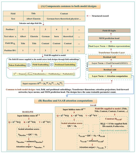
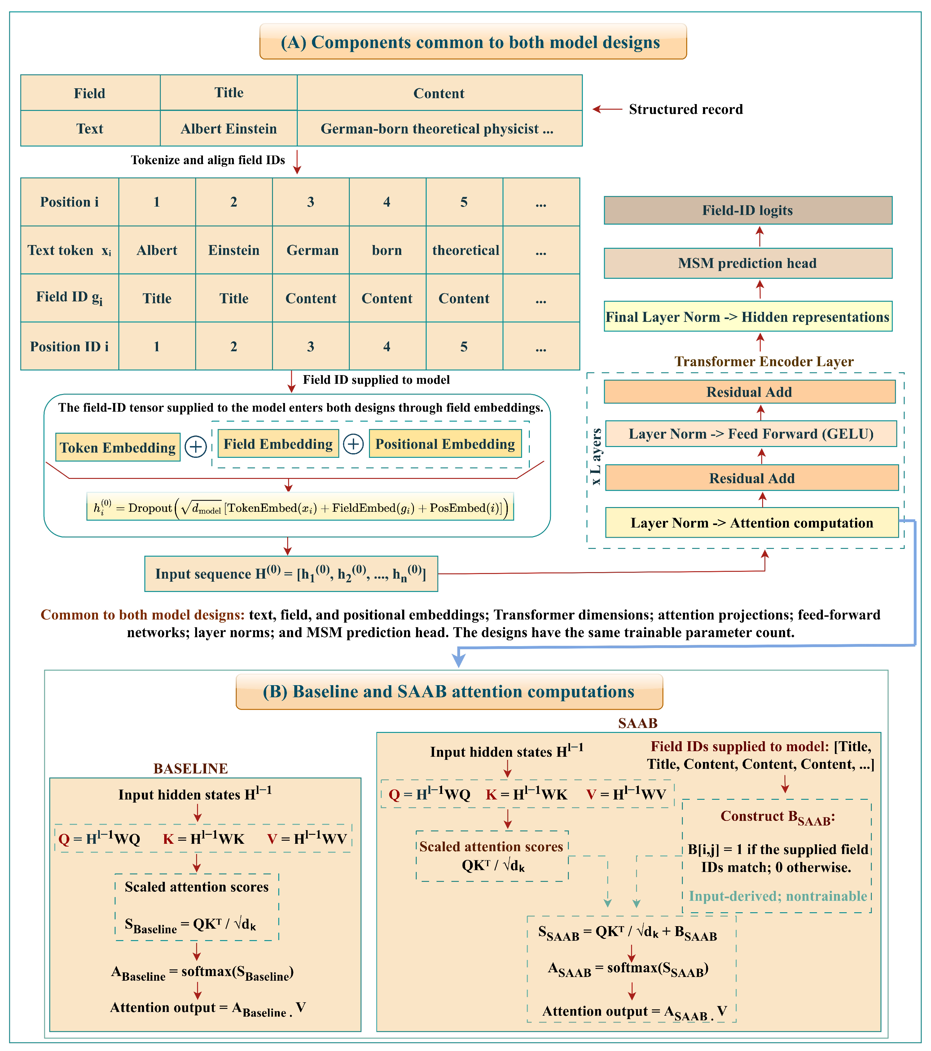
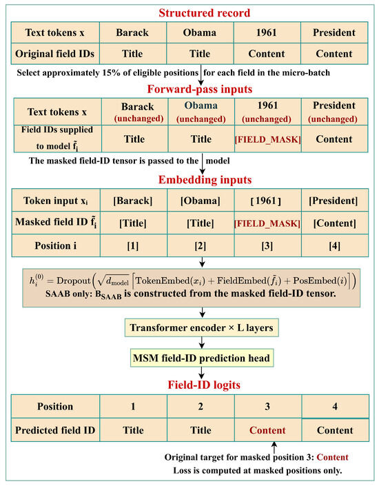
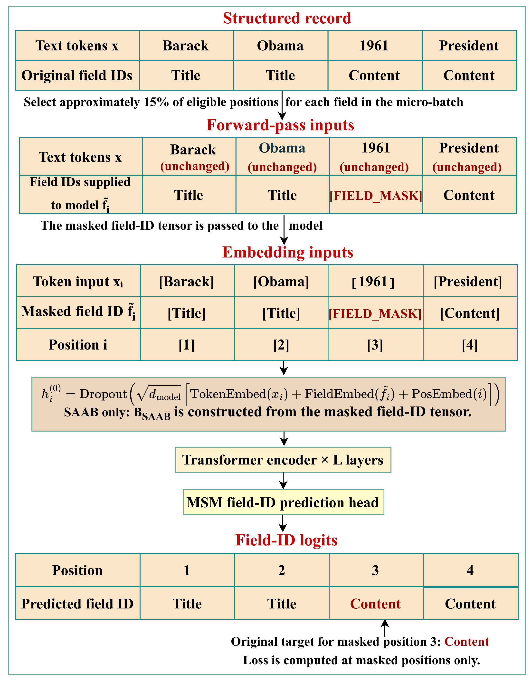
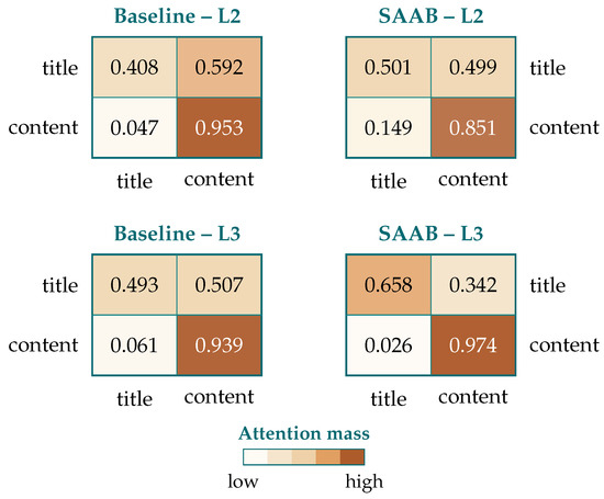
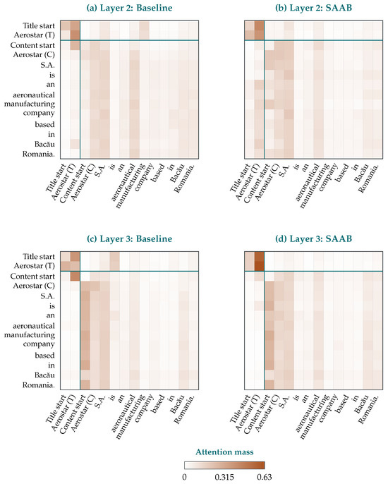
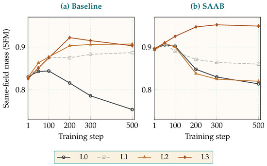
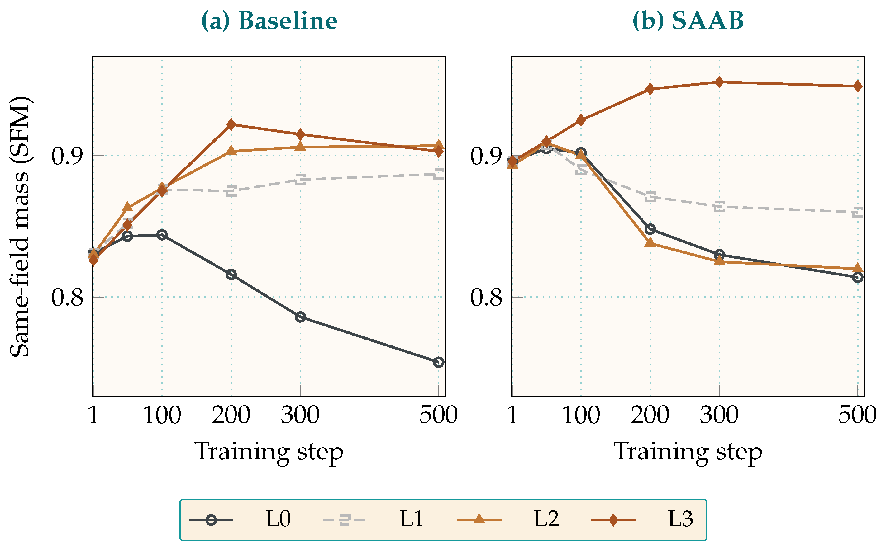
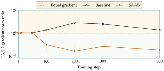
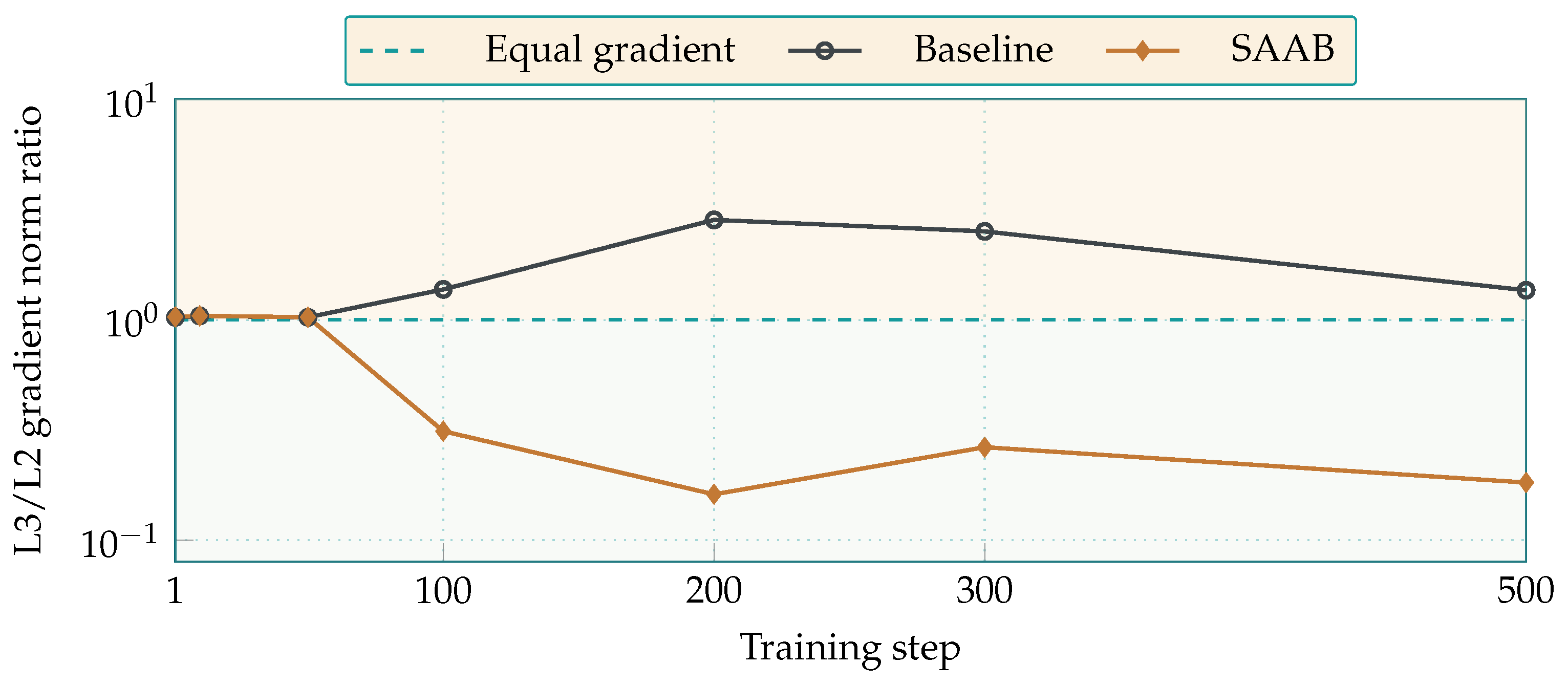
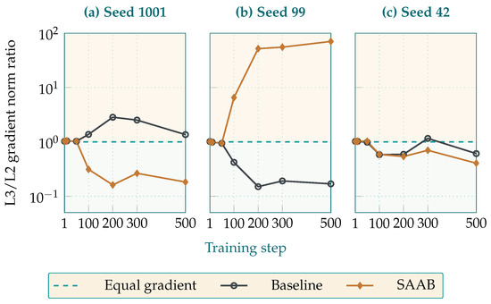
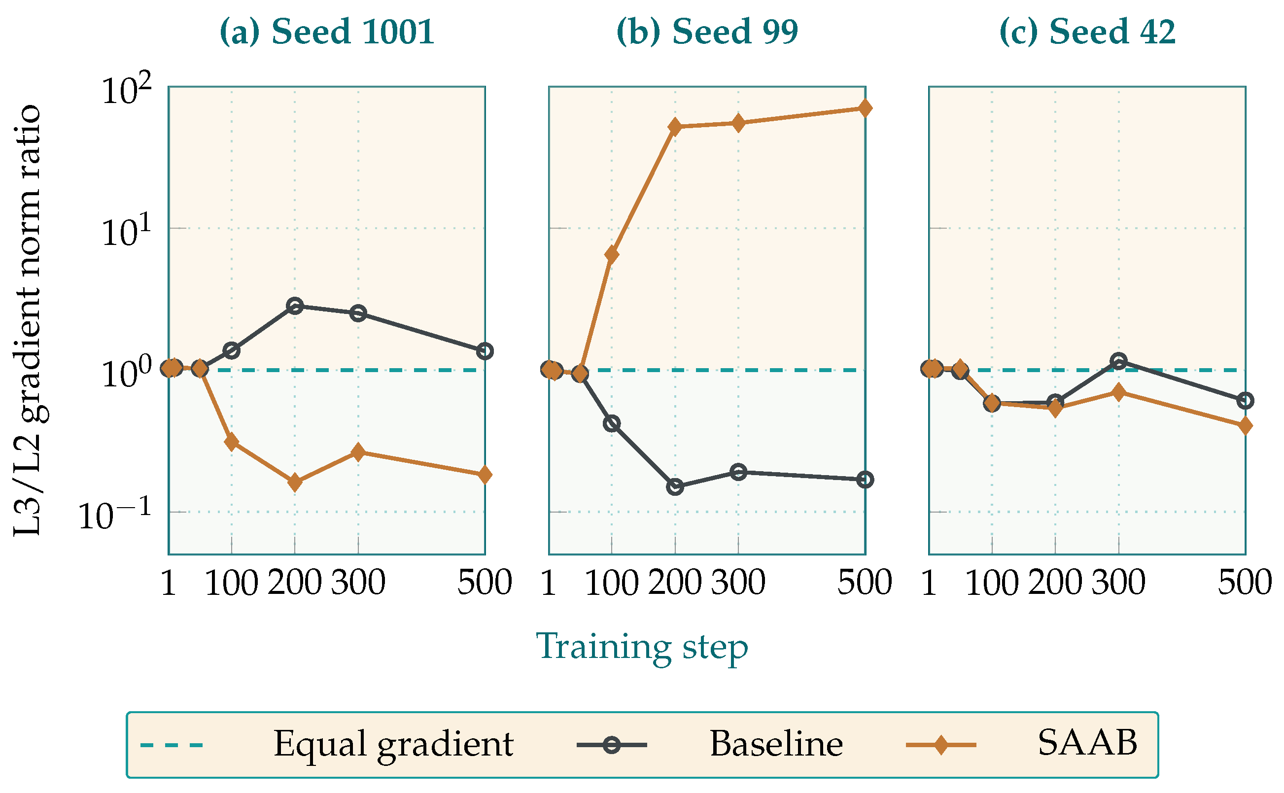
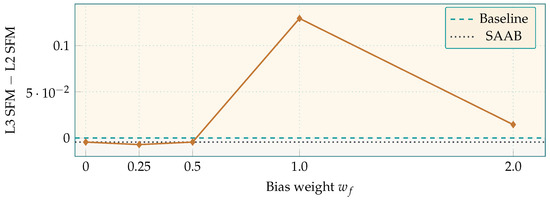
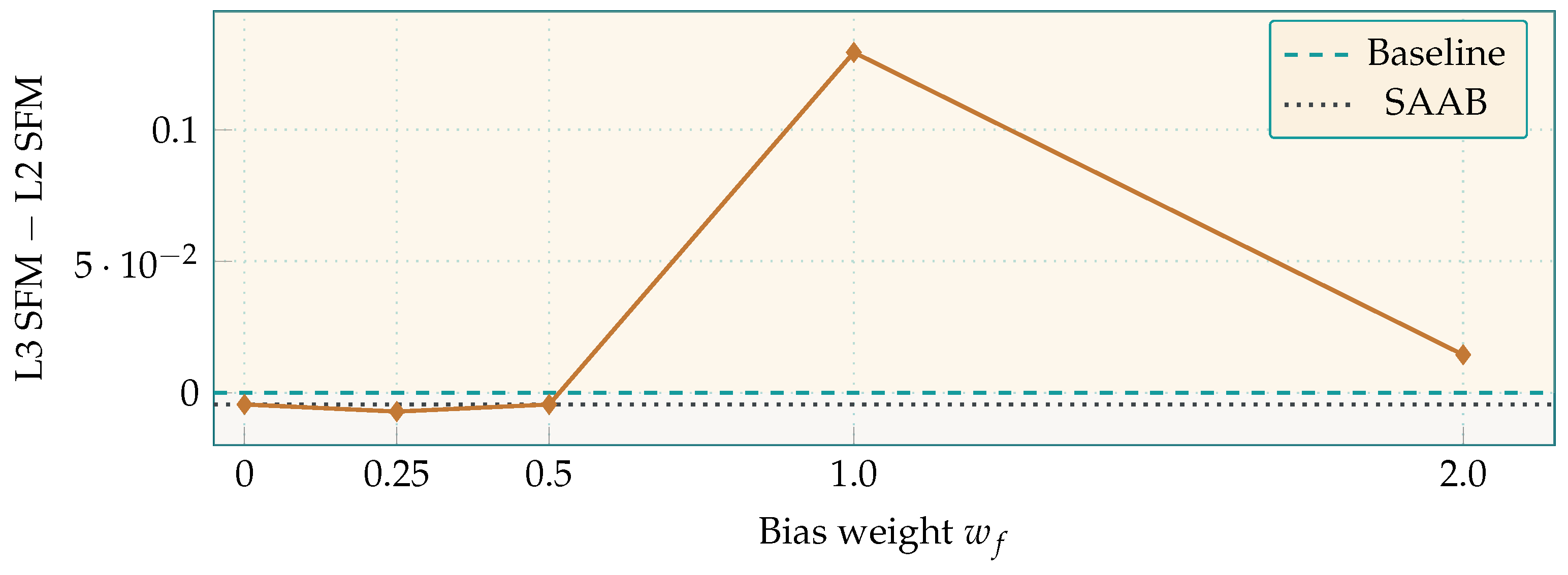
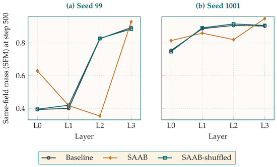

Disclaimer/Publisher’s Note: The statements, opinions and data contained in all publications are solely those of the individual author(s) and contributor(s) and not of MDPI and/or the editor(s). MDPI and/or the editor(s) disclaim responsibility for any injury to people or property resulting from any ideas, methods, instructions or products referred to in the content. |
© 2026 by the authors. Licensee MDPI, Basel, Switzerland. This article is an open access article distributed under the terms and conditions of the Creative Commons Attribution (CC BY) license.