


Featured Application
This study presents a CFD–sparse regression framework for the controlled numerical reconstruction of radon release locations and strengths in underground uranium-mine roadways. The framework provides methodological insights into source identification and future sensor-layout assessment in confined underground spaces.
Abstract
Source identification in confined underground ventilation systems is essential for hazardous-gas monitoring, and uranium-mine radon provides a representative case in which release locations and strengths must be inferred from limited concentration measurements. This presents an underdetermined, ill-posed inverse problem whose solvability under different sparse-regression strategies and roadway configurations remains poorly understood. In this study, a computational fluid dynamics (CFD) forward model is coupled with sparse regression. The ventilation flow field and radon advection–diffusion process are solved in OpenFOAM to construct a source–sensor contribution matrix, and source recovery is formulated as a sparse linear inverse problem. Four methods—LASSO, LASSO with non-negative least-squares (NNLS) refitting, Elastic Net, and Elastic Net with NNLS refitting—are compared, and the contribution matrix is characterized by its mutual coherence, condition number, and singular-value spectrum. Numerical tests were conducted for single- and multiple-source scenarios in single-main and main–branch roadway models. The results indicate that inversion performance depends on the spatial information and local identifiability provided by the sensor configuration rather than on sensor number alone. LASSO and Elastic Net exhibited varying degrees of source-strength shrinkage or dispersion, whereas NNLS refitting reduced these effects when the first-stage support contained the dominant source candidates. In the prescribed three-source case, denser sensor coverage improved dominant-source localization and reduced the post hoc condition number of the prescribed-source submatrix, although the full-matrix condition number increased. This finding indicates improved local identifiability for the tested source combination rather than a general sensor-count effect. Because the synthetic observations and the inversion operator were derived from the same CFD response matrix, the results represent a controlled model-consistent proof of concept rather than an estimate of field-level performance.
1. Introduction
Ventilation systems in confined underground spaces, such as mine roadways and tunnels, are core facilities for ensuring worker safety, and one of their primary functions is to dilute and remove hazardous gases generated or released during operations. The targeted design and optimized operation of ventilation systems depend on accurate knowledge of hazardous-gas release sources; however, in elongated, enclosed, and geometrically complex underground roadways, gas sources are often distributed across multiple locations and are difficult to detect directly. Rapidly inferring the locations and strengths of gas sources from limited monitoring data is therefore a common engineering challenge in gas monitoring for underground spaces [1].
Radon (222Rn) in uranium-mine roadways is a representative example of this problem. Radon and its progeny constitute the dominant natural radiation source for underground uranium-mine workers and have been classified by the International Agency for Research on Cancer as Group 1 carcinogens; long-term inhalation can significantly increase the risk of lung cancer [2,3]. In uranium-bearing underground mines, radon can be released from multiple locations, such as fractures in the surrounding rock, goafs, and ore piles, and its spatial distribution is sparse and difficult to detect directly. Although forced ventilation is the most effective measure for controlling underground radon concentrations [4,5], its targeted design depends on accurate identification of radon release locations and strengths [6,7]. The uranium-mine radon problem is therefore used as a representative case for developing a general source-inversion framework for confined underground ventilation systems.
After entering a roadway, radon is mainly transported by advection–diffusion within the ventilation airflow, and its concentration distribution is jointly determined by the roadway geometry and the ventilation flow field. Computational fluid dynamics (CFD) can resolve turbulent flow and passive scalar transport in complex geometries and has become an effective tool for studying gas migration and ventilation optimization in underground roadways. In the context of mine ventilation, CFD has been used to evaluate the dilution effect of auxiliary ventilation on hazardous gases in roadways and the resulting worker exposure dose [8]. Regarding radon migration in roadways, recent studies have used CFD to simulate radon exhalation and migration in roadways and surrounding rock. Chen et al. simulated radon exhalation from the surrounding rock of single and double roadways and analyzed the effects of ventilation mode and air pressure [9]. Yu et al. optimized partition-induced roadway ventilation to reduce radon concentration [10]. Lan et al. investigated flow-field zoning and radon concentration distribution in a single development roadway [11]. Ye et al. examined radon migration in surrounding rock under thermo–hydro–mechanical coupling [12]. Other studies have also simulated flow fields and radon concentration distributions in large-scale roadways during drivage [13]. These studies indicate that CFD can accurately characterize radon concentration fields in roadways and provide a basis for radon monitoring and control. However, the above studies mainly focused on the forward prediction of radon distributions from known sources, rather than inverse source reconstruction from limited concentration observations.
Inferring unknown source terms from limited concentration observations, namely source term estimation (STE), is essentially an underdetermined and ill-posed inverse problem, in which the possible source-term combinations far exceed the range constrained by observations and the solution is sensitive to noise [1]. Its solution usually relies on a forward model that describes the source–sensor relationship, and the optimal source term is determined by comparing predicted and measured concentrations [14]. Existing methods can be broadly divided into three categories: iterative optimization methods, such as Tikhonov regularization, genetic algorithms, and particle swarm optimization, which solve source parameters by minimizing a cost function [15,16]; Bayesian or probabilistic methods, which provide estimates in the form of probability distributions and quantify uncertainty but require high computational cost [17]; and machine-learning methods, such as neural networks, which have also been introduced into source term estimation in recent years [18]. When source terms are spatially sparse, compressed sensing and sparse regularization theory can be used to stably reconstruct source terms from observations far fewer than the number of unknowns [19,20]. Among these methods, the least absolute shrinkage and selection operator (LASSO) is a classical approach [21], while Elastic Net further introduces an L2 penalty to address selection instability among correlated variables [22]. With regard to radioactive source inversion, Shi et al. proposed a sparse inversion framework based on a contribution matrix and LASSO to reconstruct the distribution of radioactive sources inside a reactor building from limited dose-rate observations, and they conducted studies on spectral utilization and uncertainty analysis [23,24,25]. The idea of sparse inversion for source localization has also been applied in sensor-array signal processing [26]. Compared with fully Bayesian methods or population-based optimization methods, sparse regression transforms source-term reconstruction into a constrained linear inverse problem, offering high computational efficiency, easy repeatability, and direct use of sparse source priors. These characteristics make sparse regression a suitable choice for repeated source inversion in engineering monitoring systems. However, most contribution-matrix-based sparse inversions have been developed for radiation transport or signal localization, where the contribution matrix is determined by radiation transport or array propagation relationships. By contrast, airborne radon transport is governed by ventilation-driven advection–diffusion, and its source–sensor response relationship is jointly determined by the roadway flow field and geometry, making it fundamentally different from the above problems.
Taken together, existing studies on radon source inversion in uranium-mine roadways still have three main limitations. First, as discussed above, studies that construct a source–sensor contribution matrix based on CFD-resolved ventilation flow fields and apply it to sparse inversion of airborne radon remain limited. Second, most studies adopt a single inversion method, and systematic comparisons of the applicability and failure mechanisms of different regularization and debiasing strategies under complex roadway conditions are still lacking. Third, complex geometries such as roadway branches and junctions can significantly alter the flow field, causing different candidate sources to produce highly similar responses at the sensors, yet the influence of contribution-matrix identifiability on inversion performance has rarely been quantitatively analyzed.
To address these gaps, this study develops a CFD-informed sparse regression framework for radon source inversion in underground roadways. The ventilation flow field and radon advection–diffusion process are solved using OpenFOAM, with the standard k–ε turbulence model used to represent fully developed turbulent ventilation flow [27]. Turbulent diffusion of the passive scalar is described using an effective diffusivity that incorporates the turbulent Schmidt number [28,29]. Based on unit-source forward simulations, a CFD-derived source–sensor response matrix is constructed and then used for non-negative sparse inversion.
The remainder of this paper is organized as follows. Section 2 describes the CFD-based forward model, the construction of the source–sensor contribution matrix, the sparse inversion methods, the evaluation metrics, the numerical case design, and the CFD solver validation using the Wala benchmark case. Section 3 presents and discusses the radon source inversion results, including the identifiability of the contribution matrix, single-source and multi-source inversion performance, and the influence of sensor numbers and roadway configuration. Section 4 summarizes the main conclusions and discusses the implications for sensor deployment and ventilation-based radiation protection in uranium-mine roadways.
2. Materials and Methods
2.1. CFD-Based Forward Model for Radon Diffusion
CFD can be used to resolve the ventilation flow field and the radon advection–diffusion transport process in complex roadways. In this study, a forward model for radon diffusion is developed based on the OpenFOAM platform, and the computational procedure includes geometric modeling, mesh generation, boundary-condition specification, flow-field solution, radon-concentration transport solution, and concentration extraction at sensor locations. The unit-source response results obtained from the forward simulations are used for the subsequent construction of the contribution matrix. The overall workflow of the proposed CFD–sparse regression framework is illustrated in Figure 1. During uranium-mine ventilation, because multicomponent airflow mixing occurs in the flow field, each component must satisfy the species mass conservation law. For component i, its mass conservation equation can be expressed as follows:
Figure 1.
Flowchart of radon source inversion and reconstruction based on radon concentration monitoring data.
In Equation (1), Yi is the mass fraction of component i; Ji is the diffusion flux of component i; Ri is the net production rate of this component consumed or generated by chemical reactions per unit volume per unit time within the system; and Si denotes the net production rate of this component generated by other mechanisms, such as heterogeneous reactions and phase changes, as well as other mass source terms.
During airflow transport, fluid motion can be classified into turbulent and laminar regimes, which can be distinguished using the Reynolds number. The ventilation flow regime in a roadway can therefore be determined by the Reynolds number. When estimated using the mean air velocity at the inlet and the characteristic length of the roadway, the Reynolds number of the flow in the roadway falls within the turbulent range; therefore, the Reynolds-averaged method is adopted in this study to describe the ventilation flow field. Turbulence is an unsteady, rotational, and irregular motion of fluids and is highly complex because it varies in both time and space, causing changes in physical parameters such as temperature, velocity, and pressure; therefore, additional turbulence equations are introduced.
In the numerical simulations, the k-ε model describes turbulent viscosity by solving the turbulent kinetic energy k and its dissipation rate ε, and it is characterized by computational stability, good convergence, and mature engineering applicability, making it suitable for roadway ventilation simulations under fully developed turbulent-flow conditions [11]. The governing equations of the k-ε model include the turbulent kinetic energy k equation and the turbulence dissipation rate ε equation, which can be expressed as follows:
In the equations, k is the turbulent kinetic energy; ε is the turbulent kinetic energy dissipation rate; is the turbulent viscosity; and Gk is the production term of turbulent kinetic energy generated by the mean velocity gradient. The model constants are set as Cε1 = 1.45, Cε2 = 1.92, = 1.0, and = 1.3.
The conditions for a unique solution, including physical properties, boundary conditions, and geometric conditions, are important inputs for CFD forward simulations. Considering that this study focuses on constructing the radon source–sensor response relationship and performing source-term inversion, rather than analyzing thermal buoyancy effects induced by temperature and humidity variations, the numerical simulations assume a constant roadway temperature, constant air density, and incompressible airflow. Radon is treated as a passive scalar transported by the ventilation flow field and undergoes advection, diffusion, and decay with the airflow. In the present numerical cases, radon release is represented by prescribed interior source terms. Wall-surface flux is not independently evaluated and is therefore treated as a limitation of the current source representation. Furthermore, a passive scalar transport equation is introduced within the OpenFOAM framework, and the Reynolds-averaged Navier–Stokes (RANS) method together with the standard k−ε turbulence model is used to solve the time-averaged flow field and turbulent diffusion process. The transport equation for radon activity concentration can be expressed as follows:
where C is the radon activity concentration, SC is the source term, and λ = ln(2)/T1/2 is the radioactive-decay constant. Although decay is included in the general transport equation, it was neglected in the present steady-state simulations. For 222Rn, the 140 s ventilation traversal time gives , corresponding to a decay fraction of only 0.029%; its effect on the calculated source–sensor responses is therefore negligible. Thus, radioactive decay is retained in the governing formulation but has a negligible influence on the unit-source response matrix over the simulated roadway traversal time. The effective diffusion coefficient Deff, contributed jointly by molecular diffusion and turbulent diffusion, is defined as follows:
where Dm is the molecular diffusion coefficient of radon; is the turbulent kinematic viscosity; and is the turbulent Schmidt number. For the roadway radon simulations used to construct the contribution matrices, the turbulent Schmidt number was set to . This value lies within the commonly reported range of 0.3–1.2 for turbulent pollutant-dispersion simulations [12,13]. A value of was used separately in the Wala benchmark case, as described in Section 2.5.
2.2. Radon Source Inversion and Estimation Method
2.2.1. Construction Method for the Radon Source–Sensor Response Contribution Matrix
Based on the model established in Section 2.1, the quantitative relationship between radon release sources in uranium-mine roadways and the readings of radon concentration monitoring sensors can be constructed. It is assumed that there are n potential radon release locations in the mining area, such as fracture zones, goaf boundaries, or exposed ore surfaces, all of which may release radon into the ventilation airflow. Owing to the accessibility constraints of underground hazardous areas and the limitations of monitoring deployment conditions, only m monitoring sensors are usually installed in practical engineering applications to measure radon concentrations in roadways.
The radon source-term vector is defined as follows:
where the element xi represents the radon release rate at the i-th potential radon source location. The radon concentration measured at the j-th sensor is denoted as yj, and the corresponding monitoring vector can be expressed as follows:
The relationship between the radon source-term vector x and the monitoring vector y can be described by the contribution matrix A, as shown in Equation (8):
In these equations, denotes the actual radon release rate at the -th candidate source location, and denotes the concentration response at the -th sensor. Under a fixed ventilation flow field and with concentration-independent transport properties, the passive-scalar transport equation is linear with respect to the source term. Therefore, if is the sensor response generated by a reference release rate at candidate source , the corresponding contribution-matrix column is , and the response to an arbitrary source rate is . The total sensor response is consequently obtained by linear superposition:
This scaling relationship remains valid even when the actual source strengths differ by several orders of magnitude, provided that the ventilation field, turbulent diffusivity, boundary conditions and reaction parameters are not altered by the source magnitude. This contribution coefficient can be calculated based on the ventilation flow field and radon diffusion model described in Section 2.1, and the construction schematic is shown in Figure 2.
Figure 2.
Schematic of the radon source–sensor response contribution matrix.
2.2.2. Multi-Method Sparse Inversion Model
It is usually difficult to deploy a large number of sensors in practical engineering applications, and to reduce the cost of radon pollution monitoring and source-term identification in uranium-mine roadways, monitoring data are mainly obtained from a limited number of fixed detection points. When the potential radon source region is finely discretized into a large number of grid nodes, the dimension n of the source-strength vector to be estimated is often significantly larger than the number m of sensor observations. Therefore, the source-term–measurement response relationship shown in Equation (8) is transformed into an underdetermined system of equations, and the contribution matrix A does not satisfy the condition for direct inversion, making it difficult to obtain a unique and stable source-strength vector using conventional linear solution methods. For such ill-posed inverse problems, constrained inversion methods need to be introduced to estimate the unknown radon source-strength distribution from limited monitoring data.
In actual uranium-mine roadways, radon release is usually not uniformly distributed throughout the roadway space but is concentrated in a few localized regions with relatively strong release capacity, such as active fractures, goaf boundaries, or broken ore piles. These regions can continuously release radon into the ventilation airflow, resulting in only a small number of nonzero elements in the true source-strength vector. Therefore, even when the potential radon source region is finely discretized, the source-strength vector still exhibits clear sparsity. Based on this feature, this study constructed four non-negative sparse inversion methods, namely LASSO, Post-LASSO NNLS, Elastic Net, and Post-Elastic Net NNLS, and compared them under the same contribution matrix, observation vector, and evaluation metrics. Because the radon release rate should not be negative in physical terms, non-negativity constraints were imposed on the source-strength vector in all four methods, namely x ≥ 0. Before inversion, the contribution matrix and observation vector were normalized to reduce the influence of dimensional differences and response-amplitude differences among different sensors on the solution results. The selection of regularization parameters and screening thresholds did not use information on the true source locations or true source strengths, and the true-source information has been used only for subsequent evaluation of inversion performance.
The numerical experiments were designed as controlled model-consistent benchmarks for comparing the sparse inversion strategies and examining contribution-matrix identifiability. The synthetic observation vectors were generated from the same CFD-derived response matrix used in the inversion, without explicitly introducing measurement noise, discrepancies in structural modeling, or off-grid source mismatch. Accordingly, the numerical cases are intended to evaluate algorithmic feasibility and comparative behavior under idealized conditions rather than to estimate field-level reconstruction accuracy.
- (1)
- LASSO Sparse Inversion Method
The least absolute shrinkage and selection operator (LASSO), as a basic sparse inversion method, is suitable for sparse ill-posed inverse problems. Its core idea is to introduce an L1-norm regularization term into the least-squares residual term, thereby shrinking the coefficients of irrelevant or weakly contributing candidate sources to zero and achieving source-term selection. The optimization model of LASSO can be written as follows:
where is the LASSO loss function; represents the sum of squared residuals between the model-predicted concentrations and the sensor-observed concentrations; is the L1-norm of the source-strength vector; and is the regularization parameter used to balance the concentration fitting error and source-strength sparsity. A larger enhances sparsity but may lead to underestimation of the true source strength. A smaller helps reduce the concentration reconstruction residual but may introduce more weak spurious sources. In this study, the optimal was determined through candidate regularization-parameter search and cross-validation, and the parameter-selection process was based only on the concentration reconstruction error without using information on the true source locations or source strengths. After the solution was obtained, weak source-strength components were screened using a threshold, nonzero source grids were extracted, and the locations and release strengths of the main radon sources were determined.
- (2)
- Post-LASSO NNLS Refitting Method
While the L1-regularization term in LASSO enhances sparsity, it also shrinks the nonzero source strengths, which may result in underestimated source-strength magnitudes. Therefore, this study further adopted the Post-LASSO NNLS method for post-refitting. This method first obtains an initial sparse solution using LASSO and then extracts the nonzero support set selected by LASSO according to a weak-signal threshold:
where denotes the support used for NNLS refitting. The weak-signal threshold was defined relative to the largest coefficient in the first-stage solution as . This relative definition does not use the true source locations or strengths and avoids applying a fixed absolute source-strength cutoff across cases with different release magnitudes. The threshold controls support construction for NNLS refitting and is distinct from the post-processing threshold used only to calculate discrete detection metrics.
where denotes the submatrix of the contribution matrix composed of the columns corresponding to the support set , and denotes the source-strength vector on this support set. Post-LASSO NNLS uses LASSO as the first-stage source-location screening tool and NNLS as the second-stage source-strength refitting tool. Compared with direct LASSO, this method can reduce the source-strength shrinkage bias caused by the regularization term while preserving the sparsity of the support set, thereby improving quantitative source-strength estimation. It should be noted that the effectiveness of Post-LASSO NNLS depends on the quality of the first-stage support set. If the true source is not selected into the support set by LASSO, the second-stage NNLS cannot independently correct the missing source-location problem.
- (3)
- Elastic Net Sparse Inversion Method
In addition to LASSO, this study also uses Elastic Net as a comparative method. In uranium-mine roadways, adjacent candidate source points may produce highly similar concentration responses at the sensors, especially near branch junctions, downstream regions, or areas with insufficient sensor coverage, where strong correlations may exist among different columns of the contribution matrix. In this case, LASSO tends to select only a few source points from a group of correlated candidate sources, and the resulting support selection may be sensitive to the regularization parameter or observational perturbations. Elastic Net introduces both L1- and L2-regularization terms, thereby retaining sparse selection capability while improving estimation stability under correlated-candidate-source conditions through the L2 term. Its optimization model can be written as follows:
where is the Elastic Net loss function, is the overall regularization-strength parameter, and is the mixing regularization parameter satisfying . When , Elastic Net degenerates into LASSO. When , the model contains both an L1 sparsity term and an L2 stabilization term. The L1 term is used to shrink irrelevant source terms and enhance the sparsity of the source-strength vector, whereas the L2 term is used to alleviate support-selection instability under highly correlated candidate-source conditions. For the radon source inversion problem, Elastic Net can be used to analyze the applicability of mixed regularization under correlated-candidate-source conditions in complex roadways. However, it should be noted that Elastic Net may simultaneously retain multiple adjacent or response-similar candidate sources, appearing as source-strength dispersion or an increase in weak spurious sources in point-source localization problems. Therefore, this study uses Elastic Net as an important comparative method for LASSO to compare the effects of different regularization strategies on source-location identification and quantitative source-strength estimation.
- (4)
- Post-Elastic Net NNLS Refitting Method
To further reduce the influence of Elastic Net regularization on source-strength magnitude, this study develops the Post-Elastic Net NNLS method. This method first obtains the initial source-strength vector using Elastic Net and then extracts the nonzero support set according to a weak-signal threshold:
For Post-Elastic Net NNLS, the refit support was defined using the same relative threshold as in Equation (12), ensuring that the comparison between the two refitting procedures was not driven by different support-screening rules. Subsequently, non-negative least-squares refitting was performed on the support set selected via Elastic Net:
The purpose of Post-Elastic Net NNLS is to retain the ability of Elastic Net to screen correlated candidate sources while using NNLS to redistribute non-negative source strengths within the fixed support set, thereby reducing the source-strength shrinkage bias caused by mixed regularization. Compared with Post-LASSO NNLS, the first-stage support set of Post-Elastic Net NNLS may be broader and is more likely to include the true source or its neighboring candidate sources in regions with highly correlated responses. However, if the support set is excessively broad, the source strength may also be dispersed among multiple adjacent candidate sources, thereby increasing the risk of spurious sources. Therefore, this method is suitable for examining the applicability of a correlated-source screening and non-negative source-strength refitting strategy under complex contribution-matrix conditions.
In summary, LASSO is mainly used for sparse source-location screening, while Post-LASSO NNLS is used to correct source-strength shrinkage bias within the LASSO support set. Elastic Net is used to analyze the stability of mixed regularization under highly correlated candidate-source conditions, whereas Post-Elastic Net NNLS performs non-negative source-strength refitting on the Elastic Net support set. By uniformly comparing the four methods, this study separately evaluates the effects of sparse regularization, correlated-candidate-source treatment, and post-refitting mechanisms on radon source localization and quantitative source-strength estimation in uranium-mine roadways.
2.3. Inversion Performance Evaluation Metrics
To quantitatively evaluate the reconstruction performance of the four methods for determining radon sources, both source-location identification and source-strength estimation need to be considered. Because the source-strength vector is highly sparse, the calculation of the evaluation metrics is based on matching between the inverted sources and the true sources. For support-based evaluation, the evaluation threshold was defined as A candidate source was classified as detected when . For the reported on-grid benchmark cases, the prescribed sources were members of the same candidate-source dictionary used for inversion. Therefore, support recovery was evaluated by exact candidate-node agreement. A detected node was counted as a true positive only when its candidate-node index was identical to that of a prescribed source. No nearest-neighbor matching was allowed; equivalently, the matching radius was set to rm = 0 m.
Let N denote the number of prescribed true sources, M the number of detected source nodes, and TP, FP, and FN the numbers of true-positive, false-positive, and false-negative detections, respectively. Thus, M/N denotes the detected-to-true source-count ratio, and values greater than one indicate support over-selection.
Reconstruction quality was evaluated using complementary source-vector, observation-space, and support-recovery metrics. The source-vector metrics included the relative L2 error,
the reconstruction score, , the normalized mean absolute error,
and the spurious-source ratio,
where denotes the set of prescribed true-source nodes. Observation-space agreement was assessed using the relative residual and FAC2, defined as the fraction of sensor predictions lying within a factor of two of the corresponding observations.
Support recovery was assessed using precision, recall, and F1:
The off-grid interpolation tests were treated separately as dictionary-mismatch tests and were not interpreted as exact-node validation. These metrics were interpreted jointly because a low source-vector error does not necessarily imply correct support recovery.
2.4. Numerical Case Design
2.4.1. Geometric Model of a Single Main Roadway
The physical roadway had a cross-section of 4.0 m × 2.2 m and a length of 70 m [30]. To enable repeated unit-source simulations for constructing the contribution matrix, the computational domain was represented by a 4.0 m × 70 m reduced-order horizontal plan-view model, in which the roadway height was not explicitly resolved. The physical roadway geometry and its reduced-order horizontal plan-view representation are illustrated in Figure 3. This simplification was introduced to investigate comparative in-plane source–sensor responses under prescribed steady mechanical ventilation, rather than to reproduce the complete three-dimensional concentration field. It therefore does not assume that the concentration is vertically uniform and does not resolve roof–floor boundary layers, vertical concentration gradients, or fully three-dimensional recirculation near roadway junctions. Accordingly, the inversion results are interpreted as model-consistent proof-of-concept results for the prescribed plan-view configurations. The inlet mean velocity was set to 0.5 m s−1, and the remaining boundary conditions and physical properties were consistent with Section 2.1.
Figure 3.
Geometric model and two-dimensional simplification of the uranium-mine roadway.
The radon source was represented as a point source to characterize a localized release region, and the source location and release strength were specified using the finite-volume options module in OpenFOAM. A reference release rate of was assigned to each candidate source location, to construct a unified unit-source response matrix. This value is a calibration unit rather than an assumption that all field sources emit at . Once the unit-source response matrix was constructed, the recovered coefficient directly scaled the response to the actual source release rate at location . The linear scaling is justified because radon is treated as a passive scalar and the present model uses a prescribed steady ventilation field, concentration-independent diffusivity and linear source and decay terms. Under these assumptions, variations in ore grade, fracture density, or moisture content are represented through the spatially varying coefficients , rather than by changing the contribution-matrix construction. If a source is sufficiently strong to modify the airflow field, turbulence closure, thermal buoyancy, deposition, detector response, or other transport properties, the fixed-matrix linear model would no longer be sufficient and source-strength-dependent forward simulations would be required.
The potential radon source region was uniformly discretized at intervals of 2 m × 2 m, yielding 35 × 2 candidate source points. The detection points were arranged uniformly using a 4 × 7 = 28 layout. To analyze the influence of the source location relative to the ventilation direction with regard to the inversion results, single-point sources were placed in the upstream, midstream, and downstream regions of the single main roadway, with source locations of (1.5, 0.5), (27.5, 2.5), and (66.5, 0.5), respectively, and the source strength was set to 1 Bq s−1 in all cases.
The 2 m × 2 m discretization was used to define the candidate-source dictionary and does not imply that a physical point release must occur exactly at a grid node. To assess the effect of an off-grid point source, supplementary basis-mismatch tests were conducted for source positions located between two adjacent candidate nodes. The off-grid observation vector was constructed by linear interpolation of the neighboring unit-source response columns, , where = 0.25, 0.50, or 0.75. The same inversion dictionary containing only the original grid-node columns was then used for reconstruction.
This analysis represents an interpolation-based off-grid sensitivity test rather than an independent CFD forward simulation at off-grid source coordinates. It therefore evaluates the effect of source-dictionary mismatch under the assumption of linear response, but it does not constitute a full validation of sub-grid CFD transport.
2.4.2. Geometric Model of the Roadway with Branches
To further investigate the influence of roadway geometry on radon dispersion and source inversion, a main–branch roadway model was constructed based on the single-main-roadway configuration. The main roadway had a length of 70 m and a width of 4 m, while branch roadways with a length of 30 m were added on both sides of the main roadway. The same reduced-order horizontal plan-view formulation and scope limitations described in Section 2.4.1 were adopted for the main–branch roadway model. The model was used to examine how idealized in-plane airflow redistribution and concentration-response differences induced by the branch geometry affected radon source localization and source-strength inversion. The geometric model is shown in Figure 4.
Figure 4.
Geometric model of uranium mine roadway with branch instance.
To visually demonstrate the influence of the branched roadway structure on radon transport paths, a representative point-source case was selected for forward simulation, and the concentration-field distribution in the main–branch roadway after point-source release was obtained, as shown in Figure 5. It was observed that, under ventilation, radon was mainly transported downstream along the main roadway, and a distinct diffusion plume formed downstream of the source point. When the airflow passed through the main–branch junction, the branch structure altered the local flow field and concentration transport paths, causing part of the pollutant to diffuse into the branch-roadway regions and producing concentration-gradient variations near the junction. This phenomenon indicates that the presence of branch roadways makes the response relationship between source points and detectors more complex, and different potential source points may produce similar concentration responses at some detectors, thereby increasing the uncertainty of subsequent source-term inversion.
Figure 5.
Radon concentration field of point-source dispersion in the branched-roadway model.
2.4.3. Case-Selection Strategy and Statistical Scope
Fifteen inversion cases were selected a priori as mechanism-based benchmarks rather than as a random sample of underground mine conditions. The case set covered upstream, midstream, and downstream source locations, the main–branch junction, branch-roadway and outlet regions, as well as single-, two- and three-source configurations under different sensor layouts. This design was intended to isolate the effects of ventilation direction, roadway geometry, source multiplicity, and sensor coverage. Therefore, the results are interpreted as conditional comparisons of representative mechanisms and are not used to estimate population-level performance across all uranium-mine layouts.
Statistical robustness was assessed separately using repeated perturbation experiments. For each nonzero noise level, 50 independent Monte Carlo realizations were generated, and the median, interquartile range, mean, and standard deviation of the reconstruction metrics were calculated. In addition, 50 random 52-sensor subsets were used to evaluate the sensitivity of source recovery to sensor placement.
2.5. Validation of the Airflow–Passive-Scalar Solution Procedure Using the Wala Benchmark Case
To assess the ability of the present OpenFOAM implementation to reproduce confined-roadway airflow and passive-scalar transport, the full-scale mine-face ventilation benchmark experiment reported by Wala et al. [31] was selected as a reference case. The experiment was conducted in the NIOSH ventilation test gallery, with a roadway height of 2.2 m and a total width of 5.0 m. In the benchmark configuration, the effective ventilation region was formed by a stopping wall located 1.0 m from the right rib, and a blowing brattice curtain was installed 0.6 m from the left rib. The setback distance from the end of the curtain to the working face was 10.7 m, and the airflow rate behind the curtain was 2.8 m3/s. Methane was released near the working face and was represented in the present OpenFOAM model as a uniformly distributed multi-orifice surface source with a total release rate of 0.016 m3/s, following the CFD-equivalent treatment in the benchmark study. Methane concentrations were extracted at 36 sampling locations arranged in a 4 × 9 grid on a plane 1.0 m above the floor. The CFD-equivalent benchmark geometry and the corresponding sampling layout are shown in Figure 6.
Figure 6.
(a) Schematic of the CFD-equivalent ventilation and methane release geometry for the Wala benchmark mine working-face case; (b) layout of 36 sampling locations for the Wala benchmark case (4 × 9 grid, z = 1.0 m sampling plane).
In the present validation case, methane was treated as a passive scalar transported by the computed airflow field. Therefore, this benchmark comparison was designed to assess whether the solver can reproduce the dominant advection–diffusion pattern and concentration level in a confined mine-face ventilation flow, rather than to exactly reproduce all experimental details associated with methane release and buoyancy. The numerical model was established in OpenFOAM using a three-dimensional incompressible RANS formulation coupled with a passive scalar transport equation. The Spalart–Allmaras turbulence model was used, and the turbulent Schmidt number was set to 0.5. The SA model was adopted in the Wala benchmark to enable direct comparison with the SA-based results reported by Wala et al. [31]. Accordingly, this benchmark evaluates the OpenFOAM airflow–passive-scalar solution procedure under the benchmark configuration; it does not directly validate the Standard k−ε closure or the simplified two-dimensional radon response matrices used in the subsequent inversion cases. The turbulence closure for the roadway simulations was selected separately through the sensitivity comparison presented in Section 2.8. A velocity inlet condition was applied at the air inlet, a pressure outlet condition was imposed at the outlet, and no-slip conditions were used for the remaining walls. It should be noted that methane was introduced as an equivalent surface source perpendicular to the working face in the numerical model, whereas the experiment introduced methane through pipe holes near the face. This difference in source representation may have led to local discrepancies, particularly in regions with strong recirculation or flow separation.
The relevance of the Wala benchmark to the radon simulations is therefore limited to the shared airflow–scalar transport operator; both methane and radon are transported by advection and turbulent diffusion in the prescribed ventilation field. The benchmark provides evidence that the OpenFOAM implementation can reproduce the dominant confined-ventilation transport pattern and concentration level for a passive scalar, but it does not constitute a radon-specific validation of radioactive decay, radon exhalation physics, or source-boundary conditions. The radon-specific assumptions are justified separately by the passive-scalar approximation, the prescribed interior point-source representation, and the small decay fraction over the simulated traversal time.
To quantitatively evaluate solver performance, methane concentrations at the 36 sampling locations on the plane 1.0 m above the floor were compared with the digitized experimental data, the Fluent–Spalart–Allmaras results reported by Wala et al. [31], and the present OpenFOAM predictions obtained using the Spalart–Allmaras and standard k−ε turbulence closures. As shown in Figure 7, both OpenFOAM calculations reproduce the overall concentration level and the characteristic zigzag variation across the sampling locations. The OpenFOAM–Spalart–Allmaras prediction follows the overall experimental trend closely, while the OpenFOAM–standard k−ε calculation reproduces the main transport pattern with a somewhat different concentration amplitude at several locations.
Figure 7.
Comparison of digitized methane measurements, Fluent–Spalart–Allmaras results, and OpenFOAM predictions using the Spalart–Allmaras and standard k−ε closures at 36 sampling locations in the Wala mine-face benchmark.
Quantitative agreement between the simulated and experimental methane concentrations at the n = 36 sampling locations was assessed using fractional bias (FB), normalized mean square error (NMSE), factor-of-two accuracy (FAC2) and root mean square error (RMSE). Let and denote the observed and predicted methane concentrations at sampling location i, respectively, and let and denote their corresponding arithmetic means. The benchmark metrics were defined as follows:
where I(⋅) is the indicator function. Under the adopted FB convention, a positive value indicates overall underprediction, whereas a negative value indicates overall overprediction. FB, NMSE, and FAC2 are dimensionless, whereas RMSE is reported in methane-concentration percentage points.
The resulting statistical indicators are summarized in Table 1. The OpenFOAM–SA calculation yielded FB, NMSE, FAC2, and RMSE values of 0.182, 0.171, 0.861, and 0.168 percentage points, respectively. The corresponding Fluent–SA values were 0.246, 0.218, 0.889 and 0.184 percentage points. The auxiliary standard k–ε calculation produced FB = −0.136, NMSE = 0.178, FAC2 = 0.833, and RMSE = 0.201 percentage points. Thus, all three simulations satisfied the adopted acceptance criteria for FB, NMSE, and FAC2. However, these statistics assess agreement for the Wala methane benchmark and should not be interpreted as a complete validation of the radon-specific inverse operator.
Table 1.
Statistical comparison of methane concentrations at 36 sampling locations between CFD simulations and benchmark experiments.
The statistical indicators are listed in Table 1. The fractional bias (FB), normalized mean square error (NMSE), and factor-of-two accuracy (FAC2) between the present simulation and the experiment all fall within or close to the acceptable ranges recommended by Chang and Hanna [32]. The OpenFOAM–Spalart–Allmaras results give FB = 0.182, NMSE = 0.171, FAC2 = 0.861 and RMSE = 0.168. The Fluent–Spalart–Allmaras results reported by Wala et al. [31] give FB = 0.246, NMSE = 0.218, FAC2 = 0.889, and RMSE = 0.184. The additional OpenFOAM–standard k−ε calculation gives FB = −0.136, NMSE = 0.178, FAC2 = 0.833, and RMSE = 0.201. All three numerical results satisfy the stated FB, NMSE, and FAC2 acceptance criteria. Under the adopted FB convention, FB > 0 indicates overall underprediction, whereas the negative FB of the standard k−ε calculation indicates slight overall overprediction.
Local discrepancies remain at several sampling locations, particularly near the brattice-curtain end and the recirculation-sensitive region. These differences may arise from the steady-state approximation, the CFD-equivalent surface-source representation, and the difference between the orientation of the simulated methane source and the pipe-based injection used in the experiment. The comparison therefore supports reproduction of the dominant airflow-driven passive-scalar transport pattern, while not implying pointwise equivalence at all sampling locations.
The additional standard k−ε calculation was performed as a post hoc turbulence-closure sensitivity check using the same Wala benchmark geometry, sampling locations, and passive-scalar boundary conditions. It was not used to construct the radon contribution matrices and should therefore be interpreted as an auxiliary consistency check rather than as an independent validation of the two-dimensional radon inversion operator. The benchmark provides confidence in the general OpenFOAM implementation of coupled airflow and passive-scalar transport, but it does not directly validate radon-specific radioactive decay, radon exhalation, wall-source boundary conditions, or the reduced two-dimensional roadway representation. These remain model assumptions under the prescribed steady ventilation conditions.
2.6. Mesh Generation and Grid Sensitivity Analysis
Before conducting the forward simulations, a grid sensitivity analysis was first performed using the single-main-roadway geometry as an example. Three sets of grids with different refinement levels were established, as listed in Table 2.
Table 2.
Three grid division schemes.
The mesh study was expanded from a qualitative comparison in the main roadway to a quantitative medium–fine sensor-response-vector sensitivity analysis at five representative locations: upstream, midstream, downstream, the main–branch junction, and the remote branch. For the four observable locations, the relative response-vector difference ranged from 7.04% to 15.41%, while the response-pattern correlation remained between 0.9904 and approximately 1.0000. The junction case showed moderate sensitivity ( = 10.63%; = 6.85%; r = 0.9904). The remote-branch response was below the observability threshold; therefore, relative amplitude errors are not reported because their near-zero reference magnitude would make them uninterpretable. Its normalized response pattern was retained only for qualitative comparison and the case was excluded from amplitude-convergence claims. Accordingly, these results are reported as finite-size-source sensor-response grid sensitivity rather than strict asymptotic grid independence.
Table 2 is retained to document the coarse, medium, and fine mesh configurations. The new sensitivity table reports the resulting sensor-response changes and extends the assessment beyond the main roadway. The medium mesh was retained for the contribution-matrix calculations because it captured the dominant response pattern at substantially lower computational cost than the fine reference mesh, while the residual amplitude sensitivity is reported explicitly. Here, , is the relative difference in the maximum sensor response, and shape error is computed after optimal amplitude alignment. Table 3 summarizes the medium-to-fine sensitivity metrics for the five representative source locations. The corresponding concentration fields obtained using the three mesh levels are compared in Figure 8.
Table 3.
Medium-to-fine sensor-response-vector sensitivity for finite-size source regions.
Figure 8.
Sensitivity analysis of single-main roadway point source diffusion forward calculation grid.
2.7. Inversion, Hyperparameter Selection, and NNLS Refitting
Before inversion, each contribution-matrix column was normalized to unit L2 norm to reduce scale differences among candidate-source responses. The estimated coefficients were subsequently back-transformed to physical source strengths in . All inversion stages imposed only the physical non-negativity constraint, ; no nodewise upper bound or total-source upper bound was imposed. Elastic Net used a globally fixed mixing ratio of , where is equivalent to the parameter often denoted by in software implementations.
For LASSO and Elastic Net, 80 logarithmically spaced values of between and 1 were evaluated using three-fold spatial cross-validation. Sensors were spatially grouped and assigned to the folds in round-robin order. Within each fold, was recalculated using only the training data, and the value yielding the minimum mean validation relative-L2 error was selected. The complete parameter settings are summarized in Table 4.
Table 4.
Inversion settings and reproducibility controls.
After the first-stage LASSO or Elastic Net fitting, the support used for NNLS refitting was defined by . Coefficients below this threshold were excluded from the refit support, whereas coefficients outside the selected support were fixed to zero during NNLS refitting. Standard non-negative least-squares refitting was then performed on the selected support without an L1, L2, nodewise-bound, or total-source-bound penalty. The same relative support-screening rule was used for Post-LASSO NNLS and Post-Elastic Net NNLS.
For the noise experiments, the selected absolute was fixed across all repetitions, and every compared method received the same noisy observation within each repetition. The evaluation threshold was fixed at and was used only to determine detected sources for precision, recall, and F1; it did not modify the continuous reconstructed source vector. Ground-truth source information was excluded from screening, parameter selection, support construction, and refitting and was used only for post hoc evaluation. This fixed-threshold noise analysis evaluates perturbation stability at the selected threshold and does not imply that threshold sensitivity is absent.
2.8. Turbulence Model and Computational Parameter Settings
To assess the sensitivity of the roadway-scale radon transport results to the turbulence closure, streamwise concentration distributions obtained using the Spalart–Allmaras, k−ω shear stress transport (SST), realizable k−ε, and standard k−ε models are compared in Figure 9. The SA model predicts consistently higher concentration levels over most of the roadway, particularly in the near-source and intermediate regions, whereas the three two-equation RANS models exhibit more comparable downstream decay trends. Differences among the models are most pronounced near the source and decrease in the downstream region. Because no independent radon concentration measurements are available for this idealized roadway case, Figure 9 is interpreted as a qualitative turbulence-model sensitivity assessment rather than as a quantitative validation or accuracy ranking. The standard k−ε model was selected for the repeated unit-source simulations because of its numerical stability, computational efficiency, and engineering applicability to fully developed ventilation flows. This selection represents a practical modeling choice and does not imply that the standard k−ε model is universally more accurate than the other closures.
Figure 9.
Comparison of radon concentration distributions along the ventilation direction under different turbulence models.
2.9. Forward-Simulation Convergence and Determination of Pseudo-Time
To ensure the stability of the unit-source response results, this study conducted pseudo-time convergence analysis for the forward simulation of point-source diffusion in the roadway with branches. Six representative detection points near the outlet and in the branch-roadway region were selected, and their concentration variations with pseudo-time were recorded, as shown in Figure 10. The concentrations at each detection point changed rapidly in the initial stage and then gradually approached stable values. When the pseudo-time reached approximately 2100 s, the concentration curves essentially entered a quasi-steady state, corresponding to approximately 10,500 iteration steps. Therefore, a pseudo-time of 2100 s was used as the computational termination time for subsequent unit-source forward simulations and contribution-matrix construction.
Figure 10.
Pseudo-time convergence of point-source transport in the main–branch-roadway model.
2.10. Sensor Deployment and Contribution Matrix Schemes
Inversion analysis requires the prior construction of a source–measurement-point contribution matrix. In this study, a unit-source point-by-point forward simulation method was adopted, in which each candidate location was successively assigned as a unit radon source while the source strengths at the remaining candidate locations were set to zero, and the concentration response of that source point at each detector was obtained through CFD forward calculation to form the contribution matrix.
Sensor deployment was determined based on the ventilation flow direction, roadway geometry, and the demand for effective observational information in source-term inversion. Existing studies on pollutant source-term estimation have shown that the number of sensors, their spatial distribution, and their relative positions with respect to the pollution plume affect the estimation results of radon source location and release strength [33]. Therefore, in the single main roadway, sensors were arranged uniformly both along the ventilation direction and in the transverse direction. In the roadway with branches, detection points were arranged in the main roadway, inside the branches, near the junctions, and close to the outlets to capture airflow splitting, local retention, and concentration-response attenuation. The 52-detector scheme was used to represent limited monitoring conditions, whereas the 104-detector scheme was used to analyze the influence of denser deployment in key regions on complex multi-source inversion. In the single main roadway, 70 or 280 candidate source points were set, with 28 or 56 detection points adopted, respectively. In the roadway with branches, 115 candidate source points were set, with 52 or 104 detection points adopted. By comparing contribution matrices of different sizes, the effects of candidate-source discretization and detector number on inversion performance were analyzed.
Overall, the numbers of candidate source points and detection points jointly determine the size of the contribution matrix. A larger contribution matrix can provide richer source–measurement-point response information, which is conducive to improving the ability of LASSO inversion to identify radon source locations and source strengths, but it also increases the number of forward simulations and the computational cost. Therefore, this study constructed contribution matrices of different sizes to analyze the effects of candidate-source discretization and detection-point numbers on radon source inversion performance. The contribution matrix schemes are shown in Table 5.
Table 5.
Contribution matrix.
To separate the effects of sensor numbers from spatial coverage, an additional sensor-layout ablation was performed for the prescribed three-source main–branch-roadway case. Four layouts were compared: the original 52-sensor layout, a retrospective key-region 52-sensor layout, 50 random 52-sensor subsets sampled from the complete 104-location pool, and the full 104-sensor layout. All layouts used the same 115 candidate source locations and the same source configuration. The key-region layout was constructed retrospectively to enrich locations with informative responses for the prescribed source combination and was therefore used only as a diagnostic upper-bound layout rather than as a deployable prospective design. For each layout, the condition number of the prescribed-source submatrix, effective sensor coverage, source-reconstruction error, and support-recovery metrics were recorded.
The prescribed-source submatrix condition number was calculated as follows:
where denotes the prescribed source subset. Because is known only in the synthetic benchmark, was interpreted as a post hoc diagnostic rather than a directly deployable sensor-layout criterion. For random layouts, the median and interquartile range over 50 independent subsets were reported.
To distinguish numerical conditioning from physical observability, the response sensitivity of candidate source j was quantified by the L2 norm of its contribution-matrix column, , and by the normalized sensitivity . Candidate sources with below a prescribed observability threshold were classified as weakly observable. Accordingly, the effective source range was defined from the spatial extent of the observable candidate set, rather than inferred from the condition number. The 10−5 relative-column-norm cutoff used in the Elastic Net analysis was treated as an algorithmic weak-column screening threshold and was not interpreted as a universal sensor detection limit.
3. Radon Source Inversion Results and Analysis
3.1. Identifiability Analysis of the CFD-Derived Contribution Matrix
Before comparing different inversion methods, this study first analyzed the identifiability of the source–sensor contribution matrix constructed using CFD. Each column of the contribution matrix represents the concentration response generated at all detectors by the unit release of a specific candidate radon source. If the response columns corresponding to different candidate sources are highly similar, the inversion model may still exhibit source-location confusion, spurious-source activation, or unstable source-strength allocation, even when detector concentrations are reconstructed well. Therefore, mutual coherence μ, effective rank, the condition number of the full matrix are used to characterize its global structure. The condition number of the prescribed-source submatrix is additionally reported as a post hoc diagnostic for interpreting the inversion behavior of the synthetic multi-source cases. Because the actual source locations are unknown in practical monitoring, this submatrix metric is not directly available for prospective field sensor-layout design. The global and prescribed-source diagnostics exhibited opposite responses to sensor enrichment. For the original 52-sensor layout, the condition number of the prescribed three-source submatrix was 7.59 × 10³. This value decreased to 32.08 for the retrospective key-region 52-sensor layout and to 32.00 for the full 104-sensor layout, corresponding to an approximately 237-fold reduction relative to the original 52-sensor configuration. In contrast, the full-matrix condition number increased from approximately 2.74 × 10⁵ to 4.24 × 10⁹ when the original 52-sensor layout was expanded to the full 104-location layout. This opposite trend indicates that additional sensors improved the observability of the prescribed source directions without removing weak-response or highly correlated directions elsewhere in the complete candidate dictionary. Therefore, the reduction in should be interpreted as improved local identifiability for the tested source combination, whereas the increase in the full-matrix condition number indicates that source ambiguity may remain substantial when the active source subset is unknown.
Figure 11 presents the singular-value spectra of the column-normalized detectable dictionaries. For configurations with the same roadway geometry and candidate-source discretization, increasing the number of sensor locations increased the effective rank from 11.86 to 15.50 between Configurations 2 and 3 and from 21.36 to 26.86 between Configurations 4 and 5. However, the corresponding full-matrix condition numbers increased from 1.22 × 10³ to 3.99 × 10³ and from 2.74 × 10⁵ to 4.24 × 10⁹, respectively. Therefore, denser sensor coverage provides additional response information but does not necessarily improve the global conditioning of the complete candidate-source matrix.
Figure 11.
Singular-value spectra of the normalized source–sensor matrices under different configurations.
For the prescribed synthetic source combinations, the two-source submatrix condition numbers were 1.31 and 1.10 for Configurations 2 and 3, respectively. For the prescribed three-source case, the submatrix condition number decreased from 7588.35 under Configuration 4 to 32.00 under Configuration 5, indicating improved local separability of these three specific source-response columns. However, this submatrix is constructed using source locations known from the synthetic test and is available only as a retrospective diagnostic. This result therefore does not imply that increasing sensor numbers will improve every possible source combination. The near-unit mutual coherence and the full-matrix condition number of 4.24 × 10⁹ characterize numerical ill-conditioning and should not be interpreted as a physical radon detection distance. In the 104-sensor configuration, the detectable source-column norms ranged from 5.11 × 10⁻³ to 2.53 × 10³, indicating a large response-scale variation among candidate sources. Therefore, the effective source range is branch-specific and depends on the selected observability threshold, sensor sensitivity, and measurement noise; no single detection range expressed in meters can be inferred from alone. The corresponding identifiability metrics for the five configurations are summarized in Table 6.
Table 6.
Identifiability metrics of the contribution matrix under five different configurations.
Global matrix descriptors do not fully represent spatially varying source identifiability. Therefore, a local response-similarity analysis was performed using a 6 m source-neighborhood around each candidate source. The local coherence was calculated from the maximum normalized inner product between the response column of a candidate source and those of neighboring candidate sources within this neighborhood. Source-column norms were used to characterize local response strength, while the condition number of the prescribed-source submatrix, , was retained as a post hoc diagnostic for the conditioning of the tested source combination.
Two complementary association tests were conducted. Local coherence was compared with the spurious-source ratio because it represents support dispersion caused by locally similar candidate responses. The condition number of the prescribed-source submatrix was compared with relative source-strength error because it characterizes coefficient sensitivity after the source support has been selected.
Across the 15 established test cases, local response similarity showed a method-dependent association with source-support errors. For the first-stage sparse solutions, local coherence was positively associated with the spurious-source ratio for LASSO and Elastic Net. The association was weaker for Post-LASSO NNLS but remained nominally positive for Post-Elastic Net NNLS. Regarding source-strength accuracy, the condition number of the prescribed-source submatrix showed a strong association with for Post-LASSO NNLS, whereas the corresponding associations were not statistically significant for LASSO, Elastic Net, or Post-Elastic Net NNLS. The associations between local coherence and support dispersion are summarized in Table 7.
Table 7.
Local coherence and support dispersion.
The associations between true-support conditioning and source-strength error are summarized in Table 8.
Table 8.
True-support conditioning and source-strength error.
This association was particularly relevant near the main–branch junction, where flow separation, recirculation, and branch exchange generated locally similar response fingerprints. We therefore interpreted the junction and remote-branch cases jointly using local coherence , source-column norms, and the prescribed-source submatrix condition number , rather than the full-matrix condition number alone.
3.2. Single-Point Source Inversion in a Single Main Roadway
To examine the ability of different inversion methods to identify a single radon source in a simple roadway structure, a single-point source inversion case was first established in the single-main-roadway model. In this case, the contribution matrix constructed from the forward simulation of the single main roadway was used as the basis for inversion. Numerical simulation was used to obtain the radon concentration responses of an unknown point source at 28 detection points in the roadway, and the algorithms were then applied to invert the location and strength of the point source.
In the airflow field of the single main roadway, single point sources were arranged in the upstream, midstream, and downstream regions along the ventilation direction, with the source locations and strengths set to ((1.5, 0.5), 1), ((27.5, 2.5), 1), and ((66.5, 0.5), 1), respectively. The inversion calculation uses contribution matrix No. 2, which corresponds to 280 candidate source points and 28 detection points. Figure 12 presents the single-point source inversion results under different source-location conditions.
Figure 12.
Reconstructed source-strength distributions for single-source cases in the single-main-roadway model: (a) upstream source; (b) midstream source; and (c) downstream source.
Figure 12 presents the source-strength distributions obtained by different inversion methods for the single-point source cases in the single main roadway. Overall, when the true source was located in the upstream or midstream region, the inversion peaks obtained by all methods were mainly concentrated near the true source grid, indicating that contribution-matrix-based sparse inversion can effectively identify the radon source location under single-source conditions with sufficient response information. Both LASSO and Elastic Net were able to determine the main peak location; however, because the regularization terms imposed shrinkage on the coefficients, the inverted source strengths were lower than the true values in some cases. After NNLS post-refitting, the peak values obtained by Post-LASSO NNLS and Post-Elastic Net NNLS were closer to the true source strength, indicating that refitting can reduce the source-strength bias caused by sparse regularization within a fixed support set.
These results show that the invertibility of a point source in a single main roadway is closely related to its location in the ventilation flow field. When the source was located in the upstream or midstream region, a relatively large number of detectors remained downstream of the source, providing sufficient concentration-response information; therefore, all methods formed a distinct main peak near the true source point, and the recovery of both source location and source strength was relatively stable. In contrast, when the source was close to the downstream outlet, the normalized source-column response decreased and fewer sensors received a response above the effective observability threshold, the source contribution to the observation vector weakened, and the response differences among adjacent candidate sources decreased, leading to reduced local identifiability.
Under this weak-identifiability condition, purely regularized methods such as LASSO and Elastic Net are more likely to produce source-strength dispersion or local spurious peaks, whereas Post-LASSO NNLS and Post-Elastic Net NNLS can, to some extent, reduce source-strength shrinkage and improve source-strength concentration by refitting on the fixed candidate support. This result is consistent with the preceding global and local identifiability analyses, which indicate that inversion difficulties in weakly observable regions are associated with both local response similarity and the conditioning of the relevant source subset.
The off-grid point-source test further indicates that a source located between adjacent candidate nodes may be represented by multiple neighboring grid-node coefficients rather than by a single active node. For the observable mid-roadway case, the recovered location error remained small for LASSO and Elastic Net across the tested interpolation weights, although both methods retained multiple neighboring coefficients and their support-based F1 scores remained limited. Post-LASSO NNLS gave substantially smaller errors when the first-stage support contained both neighboring candidates; however, the near-zero errors in some cases should be interpreted cautiously because the off-grid observations were constructed from the same adjacent response columns used in the inversion dictionary. Thus, the test demonstrates consistency with linear interpolation of the point-source response rather than independent validation of arbitrary sub-grid source locations. In practical applications, repeated activation of adjacent candidate nodes should not by itself be interpreted as a distributed source; local grid refinement or interpolated response columns can be used to improve point-source localization while retaining the point-source model.
3.3. Single-Point Source Inversion in a Main–Branch Roadway
To further analyze the influence of complex roadway structures on single-point source inversion performance, six representative single-point source cases were established in the main–branch roadway geometric model. The point-source locations and strengths were set to ((20, 2), 10), ((35, 2.5), 20), ((35, 3), 7), ((35, 4), 4), ((68, −1), 4), and ((68, −2), 7), respectively. These point sources covered typical locations, including the main roadway, branch roadways, the main–branch junction, and regions near the outlet, and were used to evaluate the applicability of the four inversion methods under complex flow-field and geometric conditions. The inversion calculation uses contribution matrix No. 4, which corresponds to 115 candidate source points and 52 detection points.
Figure 13 presents the inverted source-strength distributions for six representative single-point source cases in the main–branch roadway. Compared with the single main roadway, the main–branch roadway involved more complex source locations, airflow splitting, and relative detector arrangements, resulting in more pronounced differences among the inversion results for point sources at different locations. For point sources located in the main roadway or in regions with sufficient detection responses, most methods formed a main peak near the true source grid, indicating that the contribution-matrix-based inversion model maintained good localization capability for single-source identification in complex roadways. Compared with LASSO and Elastic Net, Post-LASSO NNLS and Post-Elastic Net NNLS reduced source-strength bias in some cases, bringing the dominant-peak amplitudes closer to the prescribed source strengths. This result indicates that refitting can alleviate regularization-induced shrinkage.
Figure 13.
Inverted source-strength distributions for single-source cases in the main–branch roadway model: (a) upstream source at (20, 2); (b) midstream source at (35, 2.5); (c) source near the branch junction at (35, 3); (d) source near the downstream region at (35, 4); (e) downstream source at (68, −1); and (f) source at the branch end at (68, −28).
When the source point moved to a branch roadway, the junction region, or an area near the outlet, the inversion quality deteriorated markedly, and the degradation patterns differed among the methods. Among them, Elastic Net exhibited the most prominent bias; in cases near the junction region, its inversion results showed high spurious peaks at several non-true source grids, leading to significant overestimation of source strength. LASSO showed a lower degree of dispersion, but peak dispersion and location deviation still occurred in the branch-roadway and near-outlet cases. In contrast, the two debiasing methods that first determined the support set and then re-estimated the source strength were better able to concentrate the strength near the true source point.
These phenomena are related to the changes in radon transport induced by the main–branch roadway structure. At the main–branch junction, airflow splitting and local retention caused sources at different locations to produce similar concentration responses at the sensors, thereby reducing their distinguishability during inversion. For sources located deep in the branch roadway or near the outlet, most of the released radon is directly carried out of the roadway by the airflow, and only a limited number of detectors can effectively receive their responses, resulting in insufficient information for localization. Under these conditions, the L2 regularization in Elastic Net lacked the strong sparsity of LASSO and tended to distribute the strength of a single source among several nearby correlated locations, thereby aggravating the generation of spurious peaks in point-source cases. Methods with stronger sparsity or support-set refitting were comparatively less affected by this issue. Overall, in complex main–branch roadway structures, source-location identification remains relatively reliable, whereas quantitative inversion of source strength is more susceptible to the effects of flow-field structure and detector deployment.
Because all the cases discussed above prescribed point sources, additional neighboring coefficients were interpreted as algorithmic over-selection rather than as evidence of a physically distributed release. In particular, Elastic Net may activate several adjacent or response-similar candidate nodes because of local response correlation, even when the prescribed source contains only one active node. Therefore, the number of non-zero coefficients alone was not used to infer source morphology. A physically distributed-source interpretation would require additional regional diagnostics, such as cluster continuity, integrated source strength, and strength-weighted centroid stability, together with consistent results under threshold or measurement perturbations and independent geological or ventilation evidence. Such morphology-level validation is beyond the scope of the present point-source study. The weak branch-roadway cases were therefore interpreted as observability limitations rather than as evidence for or against a distributed source.
3.4. Multi-Point Source Inversion in a Single Main Roadway
In actual uranium-mine roadways, multiple radon release points usually coexist; therefore, it is necessary to further verify the capability of the proposed method to identify multiple sparse radon sources. In this study, two point sources were first arranged under the geometric conditions of a single main roadway, and the radon concentration responses at 28 detection points in the main roadway were used as inversion inputs together with contribution matrix No. 2, for multi-source inversion.
The locations and strengths of the multiple point sources were set to ((3, 3), 6) and ((43, 1), 10), respectively. To analyze the influence of iteration-error control on the inversion results, this study compares the multi-point source inversion results under different iteration-error tolerances.
Figure 14 presents the inversion results for the locations and strengths of the two point sources in the single main roadway. Overall, LASSO was not sensitive to the iteration error; under convergence tolerances ranging from 10−3 to 10−6, its inversion peaks consistently appeared at the two true source points, and the source strengths were close to the prescribed values. This indicates that the two-source problem in the main-roadway geometry has good separability, and the sparsity constraint imposed by L1 regularization is sufficient to accurately separate and locate the two sources. In contrast, Elastic Net was more sensitive to iteration accuracy; under relatively loose convergence conditions, it produced several diffuse secondary peaks near the true sources, and although the diffusion gradually weakened as the iteration-error tolerance became stricter, it was not completely eliminated. This difference arises because the L2 term in Elastic Net tends to distribute source strength among correlated candidate columns, and stricter convergence is therefore required to suppress this diffusion. The convergence-tolerance analysis revealed method-dependent behavior. Post-LASSO NNLS achieved accurate recovery only when the first-stage LASSO support adequately covered the two true sources, whereas Post-Elastic Net NNLS retained broad support across the tested tolerances. Therefore, NNLS refitting reduced amplitude shrinkage but could not correct inaccurate or excessively broad first-stage support. After non-negative re-estimation on the support set selected by LASSO, Post-LASSO NNLS produced main-peak strengths closer to the true values, indicating that the post-refitting step can reduce the underestimation of source strength caused by regularization while preserving the sparse localization results. Post-Elastic Net NNLS can redistribute the source strength to some extent, but its stability still depends on the quality of the support set identified in the first stage.
Figure 14.
Comparison of reconstructed source-strength distributions using different sparse inversion methods for multiple-source cases in the single-main-roadway model: (a) 10−3 iteration error; (b) 10−4 iteration error; (c) 10−5 iteration error; and (d) 10−6 iteration error.
Overall, the two-source case in the single main roadway verifies the ability of the established inversion framework to identify multiple sparse radon sources under simple geometric conditions, and it also demonstrates that the post-refitting strategy can improve the quantitative accuracy of source-strength estimation while preserving sparse localization results. Subsequent analyses further combine complex roadway structures, multi-source combinations, and changes in sensor configuration to evaluate the applicability and stability of different methods under complex working conditions.
3.5. Multi-Point Source Inversion in a Main–Branch Roadway
Under the complex geometric conditions of the main–branch roadway, a three-point source case was further established to examine the influence of complex roadway structures on inversion capability with regard to multiple radon sources. This case used contribution matrix No. 4, with a total of 52 detection points arranged in the main roadway and branch roadways. The locations and strengths of the multiple point sources were set to ((35, 2.5), 20), ((35, 5), 7), and ((68, −28), 7), respectively.
Figure 15 presents the inverted source-strength distributions for the three-point source case under the condition of 52 detection points in the main–branch roadway. Compared with the two-source case in the single-main roadway, the inversion difficulty of this case increased markedly. The three true sources were located in the main roadway, near the junction region, and in the downstream region of a branch roadway, respectively, with large differences in source strength, and the concentration responses of multiple sources were superimposed at the detectors. Under these conditions, LASSO formed a response peak near the first dominant source, but the source strength was clearly underestimated and accompanied by weak spurious peaks. Elastic Net tended to retain correlated candidate sources simultaneously, resulting in source-strength dispersion and local abnormal peaks in some regions, which indicates that correlation among candidate-source responses in complex roadways weakens the localization stability of mixed regularization.
Figure 15.
Reconstructed source-strength distributions for the prescribed three-source case in the main–branch-roadway model with 52 sensor locations.
In contrast, after non-negative refitting based on the support identified in the first stage, Post-LASSO NNLS and Post-Elastic Net NNLS improved the estimation of the dominant-peak amplitudes to some extent. Under the original 52-sensor layout, both refitting methods reduced the amplitude error but recovered only two of the three prescribed sources, with = 0.314. The weak distal-branch source remained unresolved, demonstrating that refitting could not compensate for inadequate source observability or missing first-stage support. This indicates that when the first-stage support set contains the true sources or their neighboring candidate sources, NNLS post-refitting helps reduce regularization-induced shrinkage and redistribute source strength. This result should also be interpreted in conjunction with the identifiability of the contribution matrix. The preceding analysis shows that the condition number of the true-source submatrix was high for the three-source case with 52 probes, indicating strong correlation among the response columns of the three sources and suggesting that quantitative source-strength estimation is easily affected by local matrix ill-conditioning.
Taken together, the three-source case in the main–branch roadway with 52 detection points reveals the limitations of finite sensor configurations in complex multi-source inversion. Pure sparse regularization is prone to source-strength underestimation or spurious-source dispersion, whereas the post-refitting strategy can improve quantitative source-strength estimation, although its effectiveness still depends on the quality of first-stage support selection and the local identifiability provided by the sensor configuration. This also provided a basis for the subsequent comparison of inversion performance under the 52- and 104-detection-point configurations.
3.6. Effect of Sensor Number and Spatial Coverage on Inversion Accuracy
To distinguish the effect of sensor number from that of spatial coverage, the prescribed three-source case was evaluated using four sensor configurations: the original 52-location layout, a retrospective key-region-enriched 52-location layout, 50 random 52-location subsets sampled from the complete 104-location pool, and the full 104-location layout. All configurations retained the same 115 candidate source locations, prescribed source configuration and inversion settings; only the selected sensor rows were varied. The corresponding response matrices contained 52 × 115 or 104 × 115 elements.
Figure 16 presents the inverted source-strength distributions for the prescribed three-source case in the main–branch roadway under the 104-sensor-location configuration. Both the 52- and 104-location configurations contained the same 115 candidate source locations, whereas sensor number and spatial coverage change simultaneously. Compared with the 52-location results shown in Figure 15, the reconstructed peaks under the 104-location configuration are generally more concentrated near the prescribed source locations, with improved recovery of the weak source in the distal branch roadway. This comparison indicates that the 104-location configuration provides additional source–sensor response information, although the respective effects of sensor numbers and spatial coverage cannot be determined from Figure 15 and Figure 16 alone.
Figure 16.
Reconstructed source-strength distributions for the prescribed three-source case in the main–branch-roadway model with 104 sensor locations.
From the perspective of the inversion methods, LASSO formed dominant peaks near the true-source locations, but the reconstructed strengths remained underestimated and were accompanied by several weak spurious peaks. Post-LASSO NNLS produced source strengths closer to the prescribed values when the first-stage LASSO support contained the true sources or their neighboring candidates, demonstrating the reduction of regularization-induced amplitude shrinkage through non-negative refitting. Elastic Net retained multiple adjacent or response-similar candidate sources in some regions, resulting in source-strength dispersion. Post-Elastic Net NNLS redistributed part of the dispersed strength and produced more pronounced peaks around the prescribed source locations, although its performance remained dependent on the support selected by Elastic Net.
Table 9 summarizes the sensor-number and spatial-coverage ablation for the prescribed three-source main–branch-roadway case. Under the original 52-sensor layout, both Post-LASSO NNLS and Post-Elastic Net NNLS recovered only two of the three prescribed sources, with = 0.314. In contrast, the retrospective key-region 52-sensor layout and the full 104-sensor layout enabled recovery of all three prescribed sources. The prescribed-source submatrix condition number decreased from 7.59 × 10³ for the original 52-sensor layout to 32.08 for the key-region 52-sensor layout and 32.00 for the full 104-sensor layout. Thus, the substantial improvement cannot be attributed to sensor numbers alone, because the key-region layout achieved a similar improvement without increasing the number of sensors.
Table 9.
Sensor-number and spatial-coverage ablation for the prescribed three-source case.
Across the 50 random 52-sensor subsets sampled from the complete 104-location pool, Post-LASSO NNLS achieved a median below 0.001, although its upper quartile reached 0.314. Post-Elastic Net NNLS yielded a median = 0.314, with an F1 interquartile range of 0.571–1.000. Elastic Net also retained broader support than LASSO across the tested layouts. These results indicate that spatial coverage can be as important as sensor numbers because it determines whether weak source responses are retained during support selection.
The distal-source response-column norm increased from 1.20 × 10⁻³ for the original 52-sensor layout to 0.341 for the full 104-sensor layout, whereas the column-normalized prescribed-support condition number changed only from 1.494 to 1.426. The improvement therefore appears to result primarily from enhanced physical observability of the distal source rather than from a substantial reduction in response-pattern collinearity. Because the key-region layout was selected retrospectively and the observations were model-consistent and noiseless, the near-zero refitting errors represent best-case numerical recovery and do not establish a universally optimal sensor layout or a universal distance-based detection range.
The random-layout experiment further quantified the variability associated with spatial placement. The median prescribed-source condition number was 37.08, with an interquartile range of 27.32–87.73. Thus, layouts with the same number of sensors can exhibit markedly different source-discrimination capability. Across these random layouts, log10κ(AS∗) was negatively associated with the LASSO F1 score. This association suggests that support recovery tends to deteriorate as the prescribed-source submatrix becomes more ill-conditioned, although it should not be interpreted as a universal causal relationship because the analysis used one fixed three-source configuration and 50 random subsets.
The key-region layout should therefore be interpreted as a retrospective diagnostic coverage-enrichment scenario rather than as a directly deployable sensor-placement strategy. In practical applications, the active source subset is unknown; sensor-layout design should consequently consider global dictionary diagnostics, local response coherence, source-column sensitivity, and multiple representative source configurations rather than sensor number alone.
3.7. Comprehensive Error Evaluation of Different Inversion Methods
To quantitatively compare the four inversion methods, Table 10 reports the relative source-vector error , spurious-source ratio Rspu, normalized mean absolute error NMAE, F1 score, and detected-to-true source-count ratio (M/N). The continuous metrics and NMAE quantify source-strength accuracy, whereas Rspu, F1, and M/N characterize support recovery, missed sources, and source over-selection.
Table 10.
Quantitative performance metrics for radon source inversion under different methods and test cases.
The reconstruction performance was strongly case-dependent. All four methods accurately reconstructed the upstream source, whereas the first-stage solutions retained additional candidates in several midstream and branch-roadway cases. Post-LASSO NNLS produced near-zero errors when the LASSO support contained the relevant true-source columns. In contrast, Post-Elastic Net NNLS did not consistently improve on Elastic Net. For example, in branch-roadway single-source case 3, increased from 0.526 to 0.724 after refitting, and broad supports remained in the two-source cases. Under the original 52-sensor three-source configuration, both refitting methods recovered two of the three sources with = 0.314, whereas under the full 104-sensor configuration, both recovered all three sources with < 0.001. These results show that NNLS refitting reduced regularization-induced amplitude bias only when the first-stage support contained the relevant source neighborhood.
The near-zero errors obtained in some refitting cases should be interpreted cautiously. The synthetic observation vectors and the inversion operator were constructed using the same CFD-derived contribution matrix, without independent model-form discrepancy or field-measurement uncertainty. Under this model-consistent setting, NNLS refitting can closely reproduce the observations when the selected support contains the true-source columns. Consequently, the near-zero errors represent best-case algorithmic performance and should not be interpreted as evidence of zero-error reconstruction under practical uranium-mine monitoring conditions.
Overall, LASSO generally produced sparser solutions but remained susceptible to shrinkage and local over-selection in weakly observable cases. Elastic Net more frequently retained correlated candidate sources and therefore produced broader supports. Post-LASSO NNLS provided the most consistent improvement when its first-stage support was adequate, whereas Post-Elastic Net NNLS remained sensitive to support dispersion. Measurement-noise sensitivity is examined in Section 3.8, while independent CFD-model discrepancy, boundary-condition uncertainty, and sensor loss remain subjects for future investigation.
3.8. Robustness Under Measurement Noise
Because the deterministic cases were selected to represent distinct transport and identifiability mechanisms, statistical robustness was evaluated through repeated perturbation experiments rather than by treating the 15 cases as independent random samples.
The effect of relative support screening was examined by scanning η from 10−5 to 5 × 10⁻² for three representative configurations: the multi-source main-roadway case and the three-source main–branch-roadway cases with 52 and 104 sensors. The threshold had little influence on the dominant reconstructed sources at low-to-moderate values, but it affected the number of weak neighboring coefficients and consequently influenced the support-based metrics, particularly, the spurious-source ratio and F1 score. At high threshold values, weak true-source or neighboring candidates could be removed from the refit support, resulting in larger changes in support recovery. Based on this sensitivity analysis, η = 10−3 was selected as an intermediate relative threshold that suppressed numerically weak coefficients while retaining the dominant-source support in the tested configurations.
Table 11 evaluates the robustness of the four inversion strategies under 1%, 3%, and 5% measurement noise. Fifty independent realizations were performed for every nonzero noise level, case, and method, whereas the noise-free condition was treated as a deterministic baseline. The median, interquartile range, mean, and standard deviation were used to characterize the distribution of reconstruction errors. Because the synthetic observations and inversion used the same response operator, this experiment is interpreted as an operator-consistent level-1 assessment of measurement-noise stability rather than as a validation against model-form discrepancy or field uncertainty.
Table 11.
(a). Reconstruction performance under 1% measurement noise. (b). Reconstruction performance under 3% measurement noise. (c). Reconstruction performance under 5% measurement noise.
Table 11 reports the median [Q1, Q3] obtained from 50 independent realizations at each nonzero noise level. Robustness remained strongly case dependent. At 5% noise, the upstream-source errors remained low, whereas the downstream Elastic Net and Post-Elastic Net NNLS solutions yielded = 1 and F1 = 0, indicating failure to recover the true support rather than coefficient divergence. In the branch-roadway case, LASSO produced a low source-vector error of 0.003 but an F1 score of only 0.113, showing that a small continuous reconstruction error does not necessarily imply accurate discrete support recovery.
For the two-source case, Post-LASSO NNLS reduced from 0.585 to 0.233 and Rspu from 0.435 to 0.141, whereas the Elastic Net family retained errors greater than one. Increasing coverage from 52 to 104 sensors reduced the median for all four methods, although F1 remained below unity. The noise experiments therefore demonstrate configuration-dependent sensitivity rather than universal superiority of any method.
Overall, NNLS refitting improved source amplitudes only when the first-stage support contained the relevant source neighborhood. Elastic Net regularization reduced some coefficient instability under noisy observations but did not guarantee correct source localization. The results therefore support a complementary interpretation of the metrics; , Rspu, and NMAE quantify reconstruction accuracy, whereas F1 diagnoses over-selection and missed sources. The discrete support metrics were calculated using the common evaluation threshold τeval specified in Section 2.7, while the continuous reconstruction metrics were unaffected by this post-processing threshold. Accordingly, these results demonstrate noise stability within the tested configurations but do not establish universal superiority under all multi-source mine conditions.
4. Conclusions
This study addresses the difficulty of directly identifying radon source locations and release strengths in uranium-mine roadways and develops a multi-method sparse inversion framework based on a CFD forward transport model and a source–sensor contribution matrix. Quantitative relationships between candidate radon sources and concentration responses at limited sensors were established through unit-source forward simulations, and four non-negative inversion methods, namely LASSO, Post-LASSO NNLS, Elastic Net, and Post-Elastic Net NNLS, were comparatively analyzed. Based on single-main-roadway and main–branch-roadway cases, the effects of source number, roadway structure, sensor deployment, and contribution-matrix identifiability on radon source inversion results were investigated. The main conclusions are as follows.
1. The CFD forward model and source–sensor contribution matrix incorporate the advection–diffusion response relationship of radon in the roadway ventilation field into the source inversion problem, thereby providing physical constraints for source localization and source-strength estimation under limited-sensor conditions. Compared with qualitative interpretation of concentration maps alone, the contribution-matrix framework formulates source reconstruction as a computable linear inverse problem and improves interpretability through sparse regularization and non-negativity constraints.
2. The four inversion methods exhibit distinct characteristics. LASSO selects sparse candidate-source supports but may underestimate source strength because of regularization-induced shrinkage and may retain weak spurious sources in poorly identifiable cases. Post-LASSO NNLS reduces shrinkage bias and improves quantitative source-strength estimation when the first-stage support contains the relevant source neighborhood. Elastic Net can retain correlated candidate-source information, but it may produce broadened support and dispersed source strength. Post-Elastic Net NNLS can redistribute source strength within the selected support, although its performance remains dependent on first-stage support quality. A broadened coefficient support should not, by itself, be interpreted as evidence of a physically distributed radon release. The noise experiments further showed that no method was uniformly superior across all source configurations; the benefit of NNLS refitting depended primarily on the quality of the first-stage support.
3. The single-main-roadway cases show that source identifiability depends strongly on the source–sensor arrangement relative to the ventilation direction. For upstream and midstream point sources, sufficient downstream sensor responses allow all methods to identify the dominant source region. In contrast, when a source is close to the downstream outlet, its normalized response-column magnitude decreases and fewer sensors receive an informative downstream response. The resulting weak local observability increases the likelihood of source-strength dispersion, spurious local peaks, and quantitative bias. This effect should be interpreted as a threshold-dependent loss of observable response rather than as a universal geometric detection distance.
4. Under the present two-dimensional horizontal plan-view assumptions, the main–branch-roadway cases show that branch geometry increases source-response similarity, thereby making the inverse problem more difficult. The sensor-layout ablation demonstrated that sensor count alone is not a sufficient design criterion. The prescribed-source submatrix condition number decreased from 7.59 × 10³ for the original 52-sensor layout to 32.08 for the retrospective key-region 52-sensor layout and 32.00 for the full 104-sensor layout, whereas the full-matrix condition number increased substantially for the 104-location configuration. Random 52-sensor layouts also exhibited a broad distribution of prescribed-source condition numbers and a significant negative association between log10κ(AS∗) and LASSO F1. These findings indicate that sensor deployment should jointly consider spatial coverage, local response coherence, source-column sensitivity, and representative source configurations. The observed improvement is therefore a configuration-specific retrospective result rather than evidence that increasing sensor numbers will universally improve source identification.
Taken together, the CFD-derived contribution-matrix and sparse-regression framework demonstrates the numerical feasibility of identifying dominant radon-source locations and estimating source strengths under the tested model-consistent conditions. The local-response analysis further indicates that global matrix descriptors alone are insufficient to characterize spatially varying source identifiability; local coherence, source-column sensitivity, and the conditioning of the relevant source subset provide complementary information, particularly near main–branch junctions.
The present conclusions remain subject to important limitations. The two-dimensional representation is intended for comparative analysis of ventilation-dominated in-plane source–sensor responses and does not resolve vertical concentration gradients, roof–floor boundary-layer effects, or fully three-dimensional recirculation at branch junctions. Synthetic measurement-noise stability was examined using Monte Carlo perturbations, and off-grid sensitivity was examined using interpolation-based tests; however, boundary-condition uncertainty, ventilation fluctuations, independent CFD model discrepancy, and field measurement uncertainty were not fully evaluated. In field applications, distinguishing algorithmic support dispersion from a physically distributed release would require a spatially contiguous and persistent source region, stability under reasonable threshold or measurement perturbations, and consistency with independent geological, emanation, or ventilation evidence.
Finally, the 15 deterministic cases and 50 random sensor layouts do not represent a statistically complete sample of all underground mine conditions. They provide controlled evidence for mechanism-specific behavior under the tested configurations. Quantitative transfer to practical mine roadways will require further validation using additional geometries, ventilation states, source morphologies, height-resolved three-dimensional simulations, and independently measured observations.
Author Contributions
Conceptualization, Y.W. and W.L.; methodology, Y.W.; software, Y.W.; validation, Y.W., J.J., C.W. and Z.Z.; formal analysis, Y.W. and J.J.; investigation, Y.W., J.J. and Z.L.; resources, W.L.; data curation, Y.W. and J.J.; writing—original draft preparation, Y.W.; writing—review and editing, C.W., Z.Z., Z.L., L.T. and W.L.; visualization, Y.W. and J.J.; supervision, W.L.; project administration, W.L.; funding acquisition, W.L. All authors have read and agreed to the published version of the manuscript.
Funding
This research was funded by the Doctoral Research Start-up Fund of the University of South China, grant number 5526QD022.
Institutional Review Board Statement
Not applicable.
Informed Consent Statement
Not applicable.
Data Availability Statement
The data generated and analyzed in this study, including the CFD case settings, CFD-derived source–sensor contribution matrices, synthetic observation vectors, and inversion result datasets, are available from the corresponding author upon reasonable request.
Acknowledgments
The authors acknowledge the support provided by the School of Resource Environment and Safety Engineering, University of South China. During manuscript preparation, the authors used ChatGPT (GPT-5.6-sol, OpenAI, San Francisco, CA, USA) for language editing. All generated text was reviewed and revised by the authors, who take full responsibility for the manuscript.
Conflicts of Interest
The authors declare no conflicts of interest.
Abbreviations
The following abbreviations are used in this manuscript:
| CFD | Computational fluid dynamics |
| FAC2 | Factor-of-two accuracy |
| FB | Fractional bias |
| LASSO | Least absolute shrinkage and selection operator |
| NMAE | Normalized mean absolute error |
| NMSE | Normalized mean square error |
| NNLS | Non-negative least squares |
| RANS | Reynolds-averaged Navier–Stokes |
| RMSE | Root mean square error |
| SA | Spalart–Allmaras |
| SST | Shear stress transport |
| STE | Source term estimation |
References
- Hutchinson, M.; Oh, H.; Chen, W.-H. A review of source term estimation methods for atmospheric dispersion events using static or mobile sensors. Inf. Fusion 2017, 36, 130–148. [Google Scholar] [CrossRef] [Scilit]
- Lubin, J.H.; Boice, J.D., Jr.; Edling, C.; Hornung, R.W.; Howe, G.R.; Kunz, E.; Kusiak, R.A.; Morrison, H.I.; Radford, E.P.; Samet, J.M.; et al. Lung cancer in radon-exposed miners and estimation of risk from indoor exposure. J. Natl. Cancer Inst. 1995, 87, 817–827. [Google Scholar] [CrossRef] [Scilit] [PubMed]
- United Nations Scientific Committee on the Effects of Atomic Radiation. Sources and Effects of Ionizing Radiation: UNSCEAR 2000 Report to the General Assembly, with Scientific Annexes; United Nations: New York, NY, USA, 2000. [Google Scholar]
- Sahu, P.; Panigrahi, D.C.; Mishra, D.P. A comprehensive review on sources of radon and factors affecting radon concentration in underground uranium mines. Environ. Earth Sci. 2016, 75, 617. [Google Scholar] [CrossRef] [Scilit]
- Zhou, Q.; Liu, S.; Xu, L.; Zhang, H.; Xiao, D.; Deng, J.; Pan, Z. Estimation of radon release rate for an underground uranium mine ventilation shaft in China and radon distribution characteristics. J. Environ. Radioact. 2019, 198, 18–26. [Google Scholar] [CrossRef] [Scilit] [PubMed]
- Sahu, P.; Mishra, D.P.; Panigrahi, D.C.; Jha, V.N.; Patnaik, R.L. Radon emanation from low-grade uranium ore. J. Environ. Radioact. 2013, 126, 104–114. [Google Scholar] [CrossRef] [Scilit] [PubMed]
- Huang, D.; Liu, Y.; Liu, Y.; Song, Y.; Hong, C.; Li, X. Identification of sources with abnormal radon exhalation rates based on radon concentrations in underground environments. Sci. Total Environ. 2022, 807, 150800. [Google Scholar] [CrossRef] [Scilit] [PubMed]
- Zhou, B.; Chang, P.; Xu, G. Computational fluid dynamic simulation of inhaled radon dilution by auxiliary ventilation in a stone-coal mine laneway and dosage assessment of miners. Processes 2019, 7, 515. [Google Scholar] [CrossRef] [Scilit]
- Chen, D.; Ye, Y.; Xia, M.; Shang, S.; Yan, Z.; Chung, L.K. Numerical simulations of radon exhalation from surrounding rocks of single and double underground roadways. J. Environ. Radioact. 2024, 273, 107388. [Google Scholar] [CrossRef] [Scilit] [PubMed]
- Yu, T.; Ye, Y.; Xia, M.; Liu, S.; Chen, D.; Yan, Z. Optimization of the operating parameters for radon reduction on brattice-induced cavern ventilation using CFD. J. Environ. Radioact. 2023, 265, 107223. [Google Scholar] [CrossRef] [Scilit] [PubMed]
- Lan, M.; Tang, Y.; Huang, H.; He, Y. Numerical simulation study of radon concentration distribution and influencing factors in a single-head roadway. J. Radioanal. Nucl. Chem. 2025, 334, 697–708. [Google Scholar] [CrossRef] [Scilit]
- Ye, Y.; Hong, Y.; Shang, S.; Yao, X. Numerical simulation study on radon migration in roadway surrounding rock under heat–moisture–force coupling. J. Environ. Radioact. 2025, 289, 107747. [Google Scholar] [CrossRef] [Scilit] [PubMed]
- Lv, P.; Wang, H.; Wang, X.; Zhu, K.; Li, Z.; Feng, S. Numerical simulation of flow field and radon concentration distribution in large-scale roadways during drivage. J. Contam. Hydrol. 2025, 273, 104602. [Google Scholar] [CrossRef] [Scilit] [PubMed]
- Gkirmpas, P.; Tsegas, G.; Ioannidis, G.; Vlachokostas, C.; Moussiopoulos, N. Identification of an unknown stationary emission source in urban geometry using Bayesian inference. Atmosphere 2024, 15, 871. [Google Scholar] [CrossRef] [Scilit]
- Ma, D.; Tan, W.; Zhang, Z.; Hu, J. Parameter identification for continuous point emission source based on Tikhonov regularization method coupled with particle swarm optimization algorithm. J. Hazard. Mater. 2017, 325, 239–250. [Google Scholar] [CrossRef] [Scilit] [PubMed]
- Efthimiou, G.C.; Kovalets, I.V.; Venetsanos, A.; Andronopoulos, S.; Argyropoulos, C.D.; Kakosimos, K. An optimized inverse modelling method for determining the location and strength of a point source releasing airborne material in an urban environment. Atmos. Environ. 2017, 170, 118–129. [Google Scholar] [CrossRef] [Scilit]
- Keats, A.; Yee, E.; Lien, F.-S. Bayesian inference for source determination with applications to a complex urban environment. Atmos. Environ. 2007, 41, 465–479. [Google Scholar] [CrossRef] [Scilit]
- Qiu, S.; Chen, B.; Wang, R.; Zhu, Z.; Wang, Y.; Qiu, X. Atmospheric dispersion prediction and source estimation of hazardous gas using artificial neural network, particle swarm optimization and expectation maximization. Atmos. Environ. 2018, 178, 158–163. [Google Scholar] [CrossRef] [Scilit]
- Candès, E.J.; Romberg, J.; Tao, T. Stable signal recovery from incomplete and inaccurate measurements. Commun. Pure Appl. Math. 2006, 59, 1207–1223. [Google Scholar] [CrossRef] [Scilit]
- Donoho, D.L.; Elad, M. Optimally sparse representation in general nonorthogonal dictionaries via ℓ1 minimization. Proc. Natl. Acad. Sci. USA 2003, 100, 2197–2202. [Google Scholar] [CrossRef] [Scilit] [PubMed]
- Tibshirani, R. Regression shrinkage and selection via the lasso. J. R. Stat. Soc. Ser. B Stat. Methodol. 1996, 58, 267–288. [Google Scholar] [CrossRef] [Scilit]
- Zou, H.; Hastie, T. Regularization and variable selection via the elastic net. J. R. Stat. Soc. Ser. B Stat. Methodol. 2005, 67, 301–320. [Google Scholar] [CrossRef] [Scilit]
- Shi, W.; Machida, M.; Yamada, S.; Yoshida, T.; Hasegawa, Y.; Okamoto, K. Inverse estimation scheme of radioactive source distributions inside building rooms based on monitoring air dose rates using LASSO: Theory and demonstration. Prog. Nucl. Energy 2023, 162, 104792. [Google Scholar] [CrossRef] [Scilit]
- Shi, W.; Machida, M.; Yamada, S.; Yoshida, T.; Hasegawa, Y.; Okamoto, K. LASSO reconstruction scheme for radioactive source distributions inside reactor building rooms with spectral information and multi-radionuclide contaminated situations. Ann. Nucl. Energy 2023, 184, 109686. [Google Scholar] [CrossRef] [Scilit]
- Shi, W.; Machida, M.; Yamada, S.; Okamoto, K. Uncertainty analysis of the inverse LASSO estimation scheme on radioactive source distributions inside reactor building rooms from air dose rate measurements. Prog. Nucl. Energy 2025, 184, 105710. [Google Scholar] [CrossRef] [Scilit]
- Malioutov, D.; Çetin, M.; Willsky, A.S. A sparse signal reconstruction perspective for source localization with sensor arrays. IEEE Trans. Signal Process. 2005, 53, 3010–3022. [Google Scholar] [CrossRef] [Scilit]
- Launder, B.E.; Spalding, D.B. The numerical computation of turbulent flows. Comput. Methods Appl. Mech. Eng. 1974, 3, 269–289. [Google Scholar] [CrossRef] [Scilit]
- Gualtieri, C. On the values for the turbulent Schmidt number in environmental flows. Fluids 2017, 2, 17. [Google Scholar] [CrossRef] [Scilit]
- Weerasuriya, A.U.; Longo, R.; Zhang, X.; Cotteleer, L.; Parente, A. Comprehensive evaluation of constant and variable turbulent Schmidt numbers for CFD simulation of near-field air pollutant dispersion. Build. Environ. 2025, 270, 112493. [Google Scholar] [CrossRef] [Scilit]
- Dai, J.; Shi, J. Reliability analysis of tunnel ventilation based on the mechanism of radon exhalation in uranium mines. Nucl. Tech. 2015, 38, 010206:1–010206:5. (In Chinese) [Google Scholar] [CrossRef]
- Wala, A.M.; Vytla, S.; Taylor, C.D.; Huang, G. Mine face ventilation: A comparison of CFD results against benchmark experiments for the CFD code validation. Min. Eng. 2007, 59, 49–55. [Google Scholar]
- Chang, J.C.; Hanna, S.R. Air quality model performance evaluation. Meteorol. Atmos. Phys. 2004, 87, 167–196. [Google Scholar] [CrossRef] [Scilit]
- Gkirmpas, P.; Barmpas, F.; Tsegas, G.; Efthimiou, G.; Tremper, P.; Riedel, T.; Vlachokostas, C.; Moussiopoulos, N. An evaluation of the sensitivity of a source term estimation methodology of sensor configuration in an urban-like environment. Atmosphere 2024, 15, 1512. [Google Scholar] [CrossRef] [Scilit]
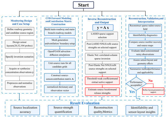
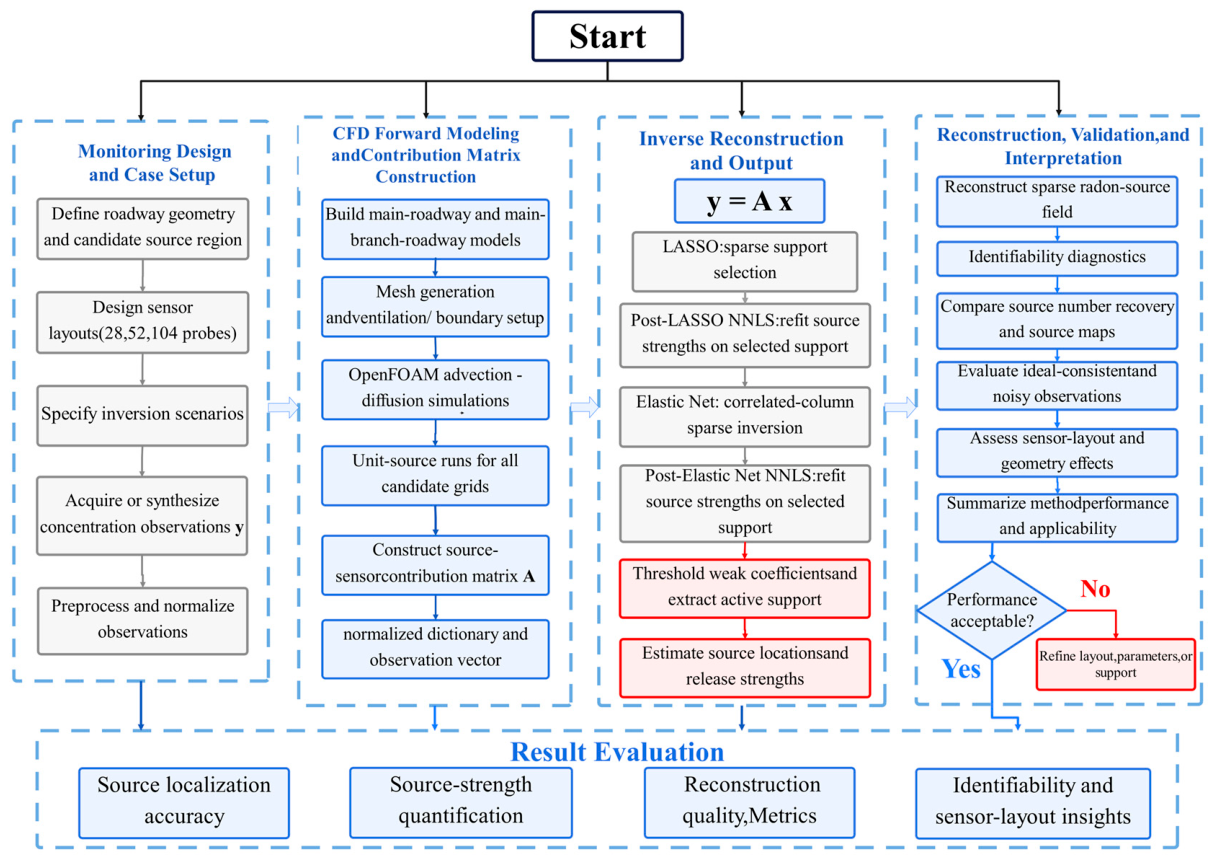
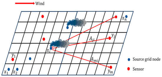
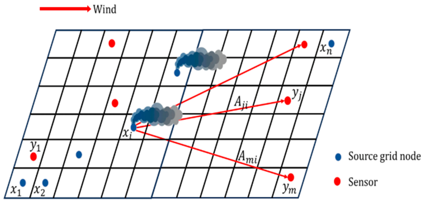
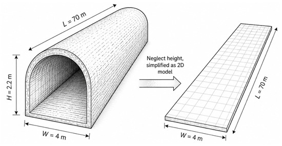
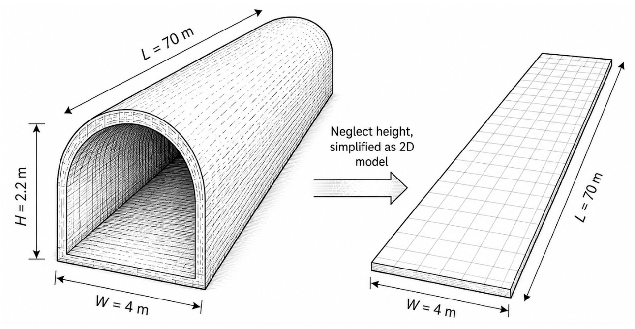
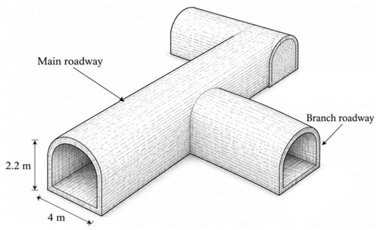
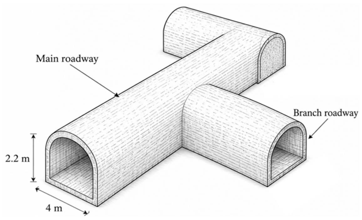
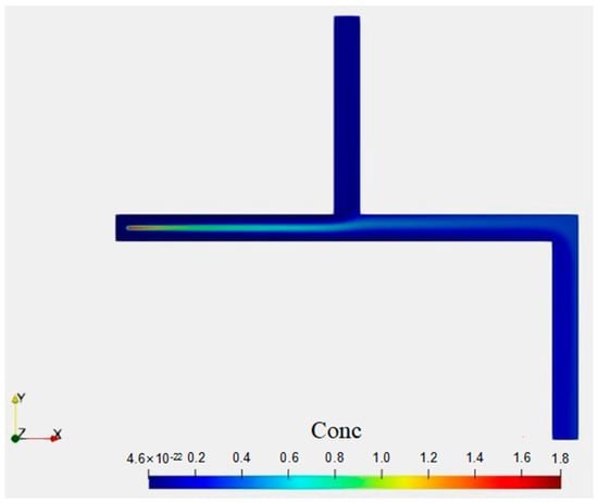
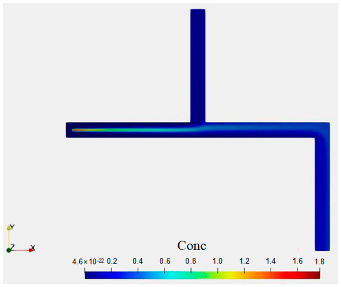
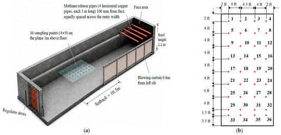
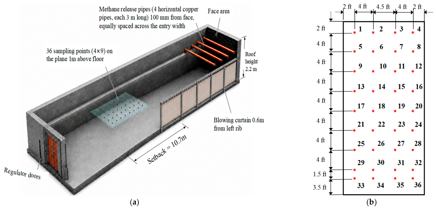
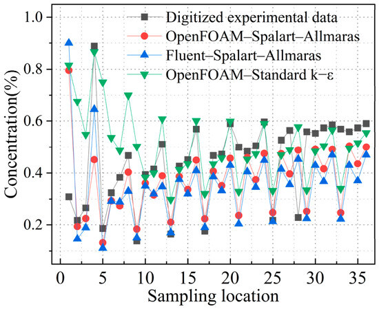
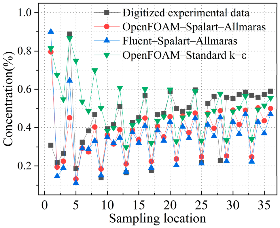
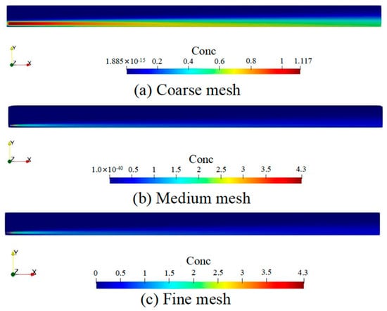
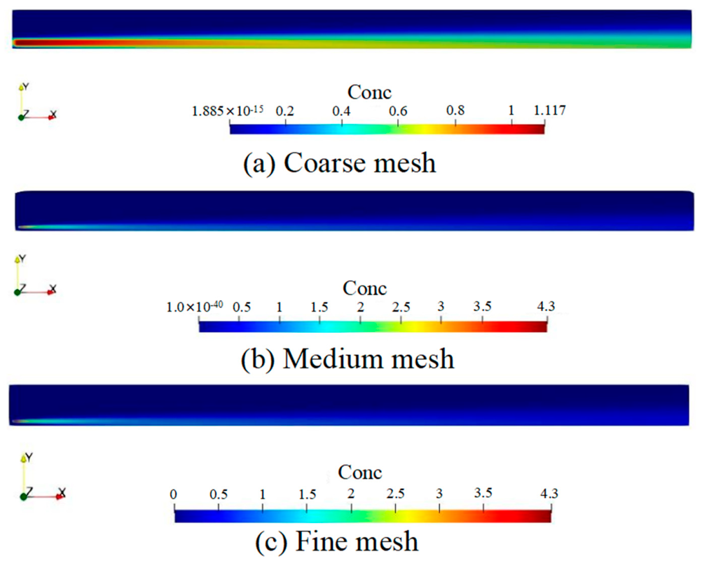
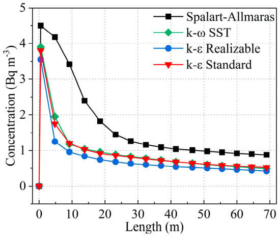
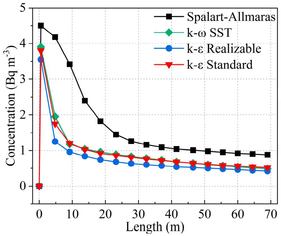
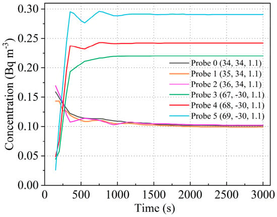
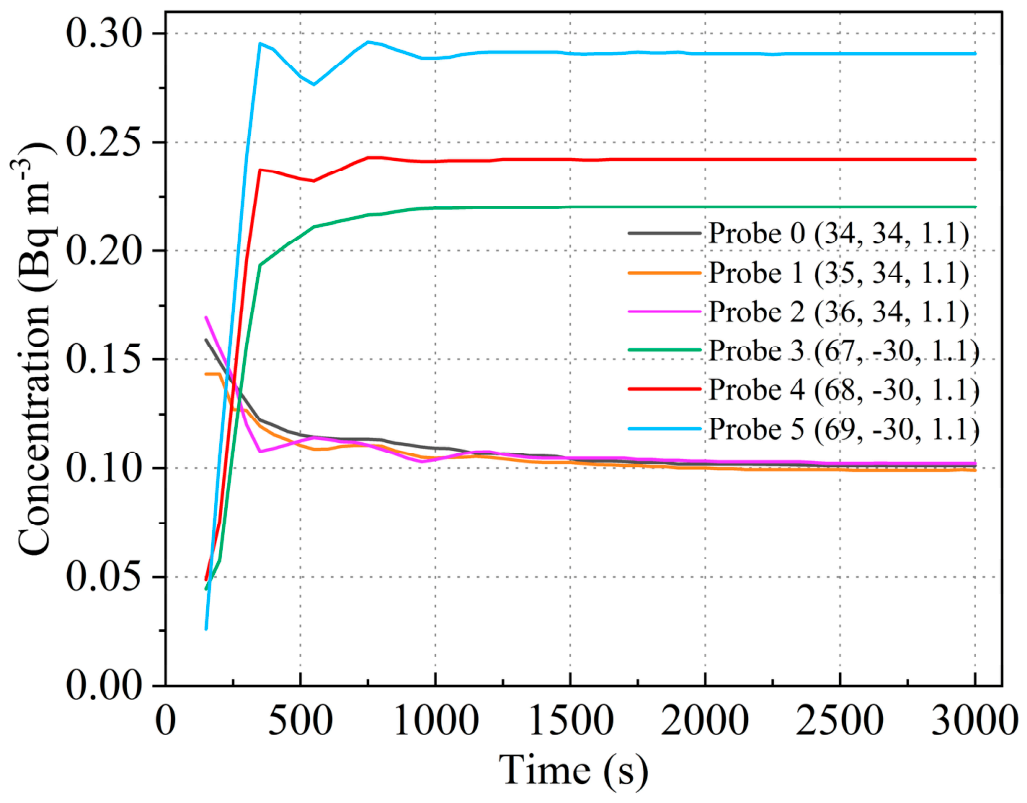
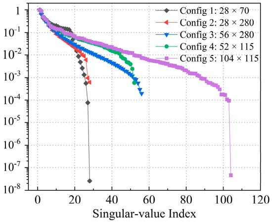
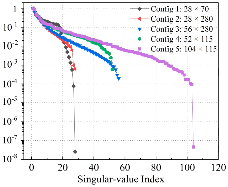
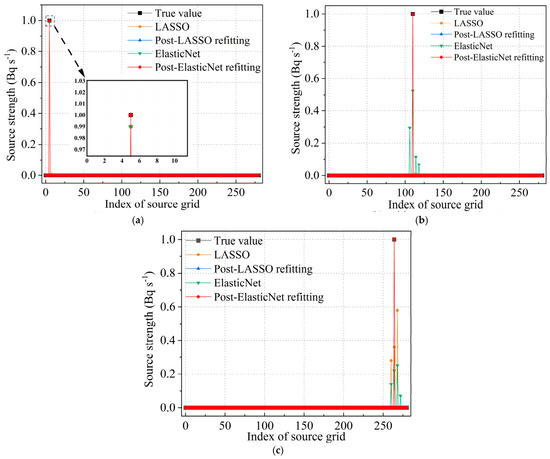
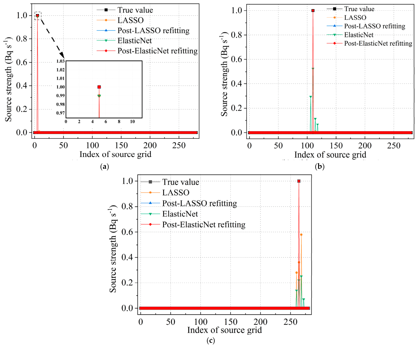
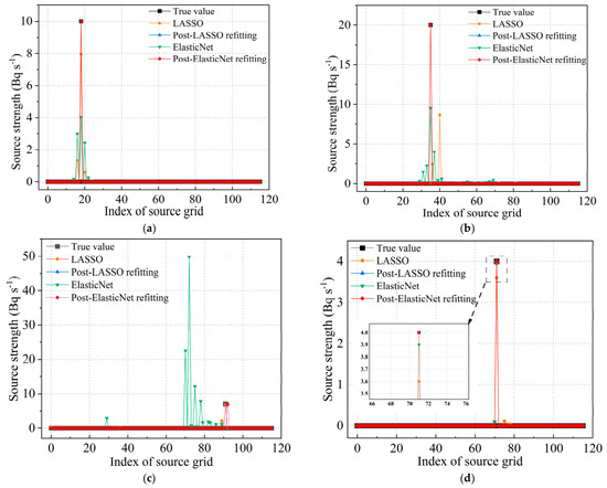
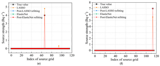
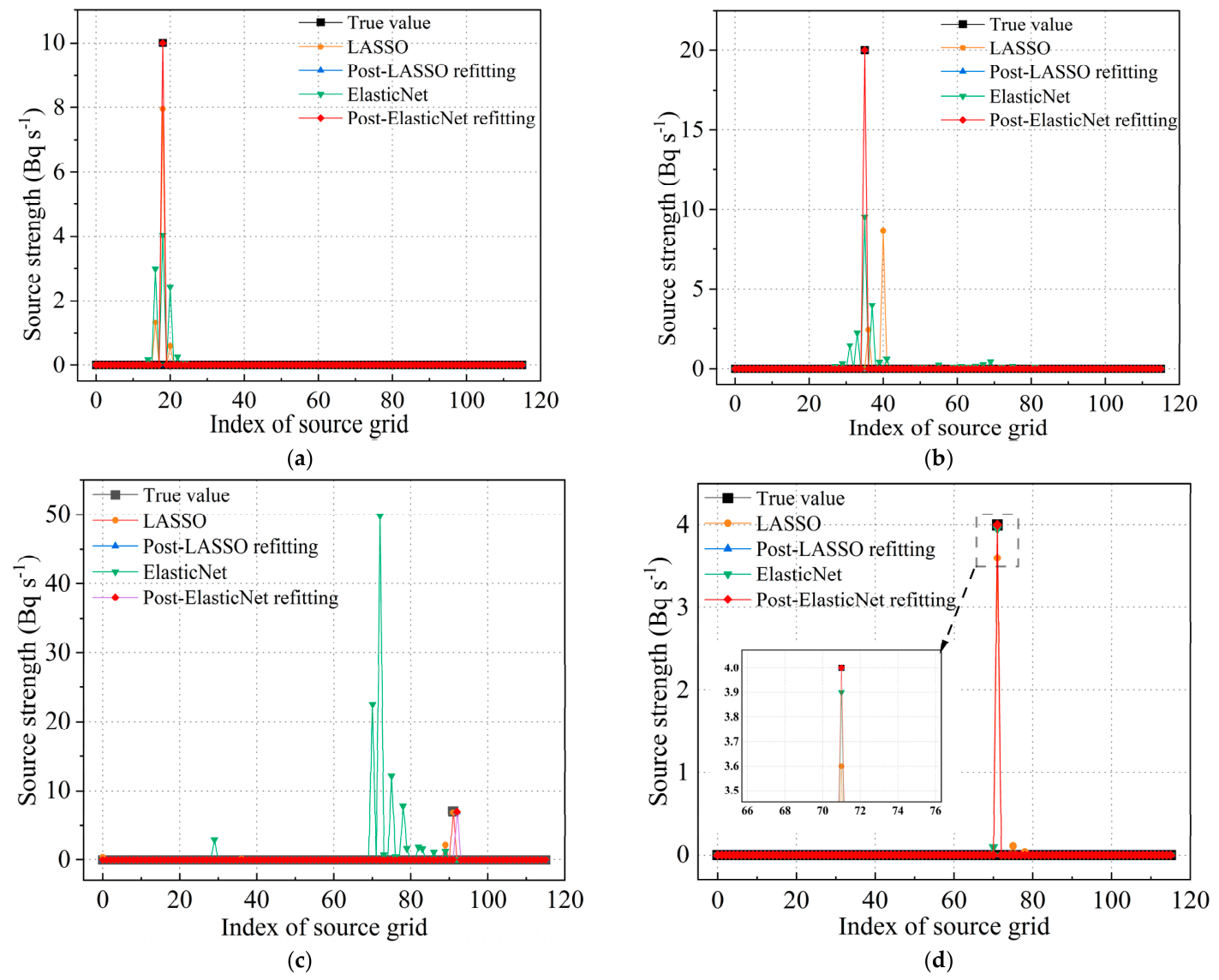
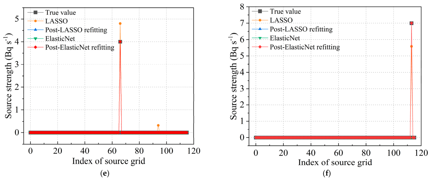
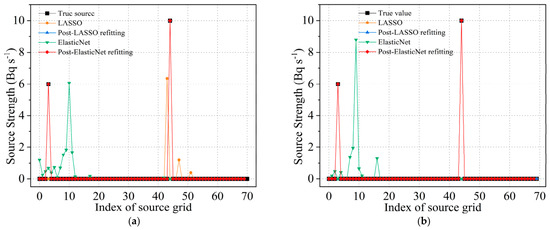
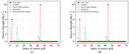
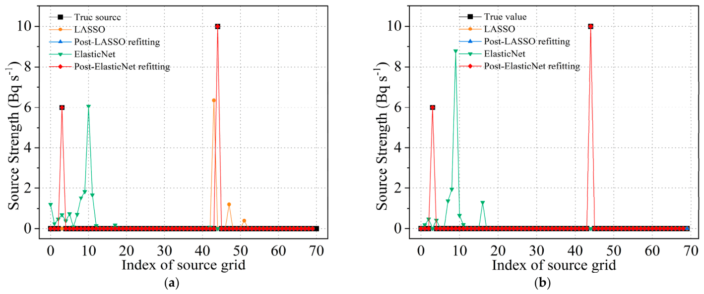
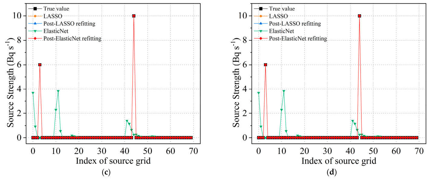
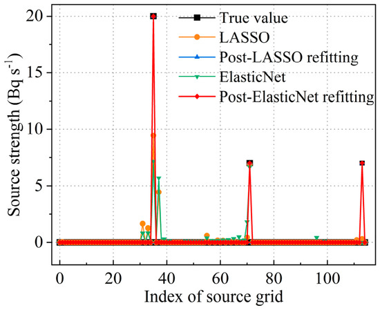
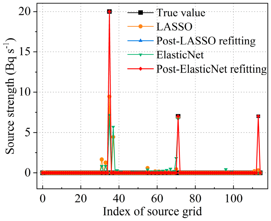
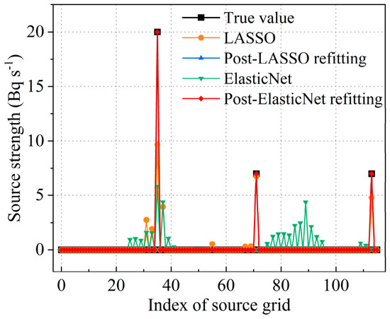
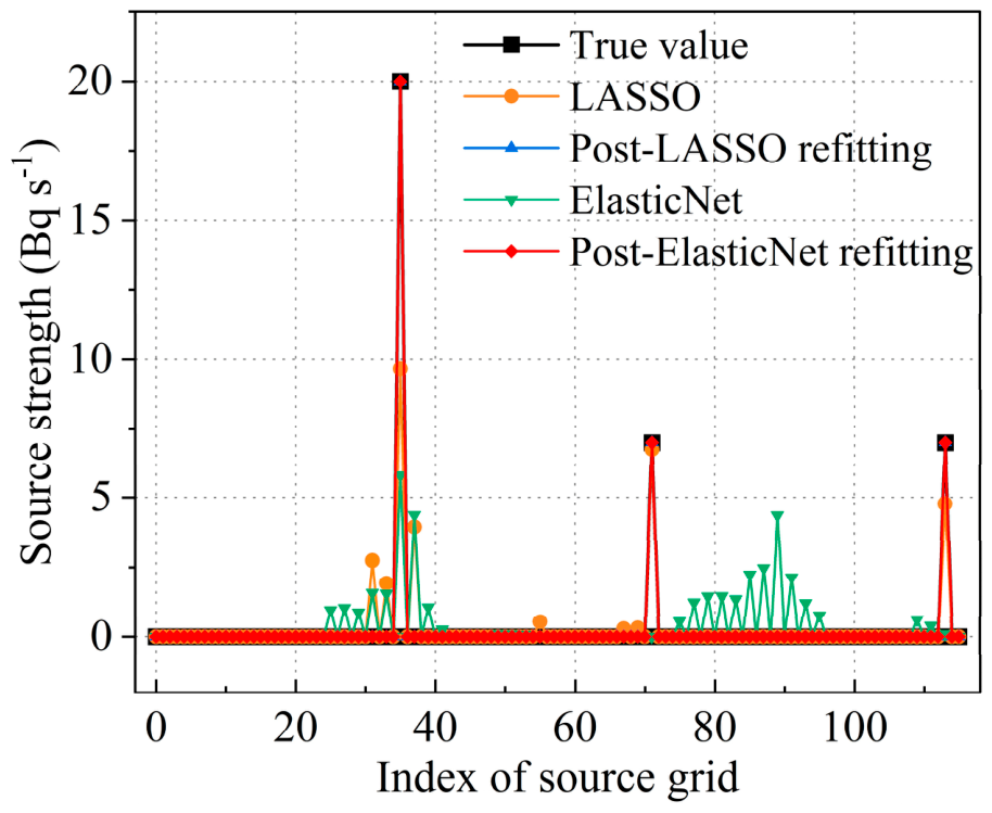

Disclaimer/Publisher’s Note: The statements, opinions and data contained in all publications are solely those of the individual author(s) and contributor(s) and not of MDPI and/or the editor(s). MDPI and/or the editor(s) disclaim responsibility for any injury to people or property resulting from any ideas, methods, instructions or products referred to in the content. |
© 2026 by the authors. Licensee MDPI, Basel, Switzerland. This article is an open access article distributed under the terms and conditions of the Creative Commons Attribution (CC BY) license.