


Abstract
Oilfield production forecasting serves as the decision-making basis for monthly production allocation and injection–production system optimization. Existing mainstream prediction methods face significant limitations: the Arps decline curve extrapolates historical production trends, yet its accuracy degrades rapidly following adjustments to injection–production regimes; machine learning methods such as XGBoost can leverage extensive dynamic data but rely heavily on manual feature engineering and offer limited decision interpretability. This paper proposes the FTT-Transformer prediction model, whose core innovation is the Feature-Time Tokenizer (FTT). The FTT projects every scalar pair (time step, feature) in a multivariate time series matrix into a token of uniform dimensionality, superimposing three types of positional information—time embedding, feature embedding, and global position encoding. On this foundation, a multi-head self-attention mechanism performs end-to-end, full-capacity learning of nonlinear interactions across both the temporal and feature dimensions. The model is lightweight, requiring only 35,361 parameters for 13 input features and is readily deployable. Validation was conducted using production data from two independent waterflooding oilfields. On Dataset 2 (60 wells, 2012–2026), the model achieved an R2 of 0.819, achieving performance on par with XGBoost (0.813; DM test p = 0.620, indicating no statistically significant difference) and substantially outperforming temporal Transformer baselines PatchTST (R2 = 0.683) and iTransformer (R2 = 0.786). On Dataset 1 (96 wells), it reached an R2 of 0.930, statistically indistinguishable from XGBoost’s 0.943 (DM test p = 0.611). Five-fold temporal cross-validation yielded a mean R2 of 0.840 ± 0.036, confirming the model’s stability. Ablation experiments revealed that global position encoding contributed most significantly, with its removal causing a 3.9 percentage point reduction in R2 on Dataset 2. Composite feature-importance analysis showed that monthly liquid production and water cut are identified by the model as the two most predictive features, contributing 31.93% and 30.17% of the total importance, respectively. Multi-step forecasting results demonstrated that the model retains an R2 of 0.640 for predictions two months ahead, spanning one complete decision cycle of monthly production reallocation. The proposed architecture is not domain-specific; by adapting the feature embeddings and time encoding, it could potentially be extended to diverse multivariate time series forecasting applications. However, cross-domain validation remains future work.
1. Introduction
Accurate crude oil production prediction is critical to oilfield development management. As noted by Kavuba et al. [1] and Hui et al. [2] in their comprehensive reviews, production forecasting exerts a direct influence on the decomposition of development indicators, adjustment of injection–production parameters, selection of well intervention candidates, and medium-to-long-term development planning. In waterflooding reservoirs, the principal factors affecting crude oil production include water-injection volume, reservoir pressure, water cut, and liquid production intensity. These dynamic parameters are numerous, strongly coupled, characterized by multiple time lags and inter-well interference, making it difficult for conventional methods to deliver dynamic predictions with both high accuracy and high timeliness.
1.1. Traditional Production Forecasting Methods and Their Limitations
Production forecasting methods in petroleum reservoir engineering can be broadly classified into two categories: empirical methods and numerical simulation methods. Empirical approaches, epitomized by the Arps decline curve analysis, fit exponential, hyperbolic, or harmonic decline trends to historical production data for extrapolative forecasting. Kongkiatpaiboon [3] introduced machine learning into decline curve analysis, enhancing the applicability of traditional methods; Rahman et al. [4] conducted a systematic analysis of pressure and production data using decline curves and type curves; and Pan et al. [5] further proposed a Mittag-Leffler function decline model tailored for multi-layered unconventional oil reservoirs. Collectively, these methods have evolved from empirical formulations into approaches with improved reservoir adaptability.
Empirical methods are conceptually simple and computationally convenient, and they remain widely used as rapid estimation tools in field operations. However, they are fundamentally a purely data-driven trend-fitting exercise that entirely neglects the influence of dynamic factors such as injection–production regime adjustments and reservoir heterogeneity. When production operations change—through measures such as injection stimulation, water shutoff, or well shut-in—the production decline behavior shifts, and the prediction error of empirical methods increases accordingly, rendering them incapable of guiding dynamic field adjustments.
Numerical simulation methods are grounded in porous flow theory and rely on fine-scale geological models with discrete numerical solution schemes to quantitatively characterize subsurface oil–water two-phase flow behavior. Zeedan et al. [6] provided a comprehensive comparative review of machine learning approaches in reservoir simulation; Alaidany et al. [7] proposed a machine learning-based optimization framework for gas injection and enhanced oil recovery. Commercial simulators such as ECLIPSE and CMG have been widely adopted in industry practice following their maturation. Numerical simulation offers a clear physical mechanism and can portray production variation patterns under different development scenarios. Nevertheless, its practical deployment entails significant barriers: (1) high modeling complexity—constructing a fine-scale numerical model for an oilfield requires starting from geological modeling, followed by history matching, a process that takes weeks to months; (2) substantial computational cost—a single simulation run typically requires several hours to days, failing to meet the rapid-decision demands of monthly production allocation or weekly injection adjustment in routine operations; and (3) insufficient data availability—many small-to-medium oilfields lack the comprehensive input data required for full-field high-fidelity simulation.
1.2. Advances and Bottlenecks of Machine Learning Methods
In recent years, machine learning techniques have opened new technical pathways for production forecasting. Jiang et al. [8] utilized a meta-learning-enhanced Random Forest ensemble for short-term oil well production prediction; Abed and Alshayeji [9] adopted a hybrid XGBoost-LSTM model and achieved favorable results on the Volve field dataset. These ensemble learning algorithms can effectively capture the nonlinear relationships inherent in tabular data and have outperformed traditional empirical methods in production forecasting tasks across several oilfield blocks.
Nevertheless, machine learning algorithms suffer from two principal shortcomings. First, they exhibit a strong dependency on feature engineering: intermediate transformed features such as injection–production ratio, water-cut variation rate, rolling statistics, and lagged terms must be manually extracted by reservoir engineers. The quality of these features directly determines prediction performance, and differences in feature design across engineers can lead to substantial variation in forecasting outcomes. Second, tree-based models represent features from different time steps as an unstructured set of input variables, lacking the capacity to explicitly learn the sequential dependencies and temporal dynamics across different time periods.
Recurrent neural networks (RNNs) and their variants have filled the gap in temporal sequence modeling. Ning et al. [10] compared the performance of ARIMA, LSTM, and Prophet for oilfield production time series forecasting; Zhang et al. [11] applied a CNN-BiLSTM architecture to production prediction for shale oil horizontal wells. Gated recurrent neural networks, in particular, can retain long- and short-term dependencies within sequences and have been widely applied to single-well production time series forecasting. However, RNNs present an unavoidable limitation in information aggregation: they compress the inputs of multiple variables into a single hidden state vector, bundling together the influences of different features across the temporal dimension. This precludes the separation of individual and interactive contributions of each feature to the prediction output, and long-sequence training is susceptible to gradient vanishing and information loss.
1.3. Development of Temporal Transformers and the Multivariate Adaptation Gap
Transformer architecture, with its capacity for global modeling through multi-head self-attention, achieved tremendous success in natural language processing before gradually being generalized to time series forecasting. Cornelio et al. [12] applied Transformers to behavior-centric production forecasting in unconventional reservoirs, demonstrating the potential of the self-attention mechanism in reservoir engineering; Lu et al. [13] presented a comprehensive survey of deep learning for time series forecasting, systematically reviewing the applicability of various architectures. The self-attention mechanism enables direct connections between any two positions in a sequence, simultaneously capturing long-range dependencies and local interactions. In principle, this permits the joint treatment of both “temporal evolution” and “feature coupling” in production forecasting.
However, applying the standard Transformer directly to multivariate time series forecasting is problematic. The standard Transformer is designed for one-dimensional token sequences, relying solely on token position encoding to distinguish the order of elements within the sequence. Multivariate time series, in contrast, possess a two-dimensional structure spanning the temporal and feature dimensions. For instance, “water cut at time t-1” and “tubing pressure at time t-1” represent two different physical quantities at the same time step, whereas “water cut at time t-1” and “water cut at time t-6” represent the same physical quantity at different time steps. These carry entirely distinct physical semantics. Flattening the two-dimensional matrix into a one-dimensional sequence as Transformer input conflates these two types of distances, preventing the model from distinguishing between inter-feature interactions and inter-temporal dependencies as fundamentally different patterns.
Existing temporal Transformer models have not fundamentally resolved this issue. Taleblou [14] compared the performance of deep learning architectures including Informer and Autoformer in time series forecasting; Liu et al. [15] combined CNN with iTransformer, incorporating geological and engineering constraints for production prediction in fracture-vuggy carbonate reservoirs; Zhou et al. [16] proposed DFG-PatchTST, a dynamic fusion gated patch Transformer for multicomponent time series forecasting. The above models were primarily designed from the perspective of long-sequence univariate or few-variate predictions. In multivariate settings, they adopt channel-wise concatenation of input features, implicitly treating all features as semantically equivalent. Information encoding the distinct identity of each dimension is neither explicitly represented nor differentiated by the model, making it difficult to fully exploit the heterogeneous relationships among different features in multivariate data.
Relationship to the Tabular FT-Transformer. It should be noted that the name “FT-Transformer” was previously used by Gorishniy et al. [17] to denote a Feature Tokenizer-based Transformer for tabular data classification. To avoid confusion, we rename our model to FTT-Transformer (Feature-Time Tokenizer Transformer). Despite the shared high-level concept of “feature tokenization,” the two models differ fundamentally: (1) input structure: the tabular FT-Transformer treats each sample as a set of k static features, producing k tokens for a permutation-invariant table; FTT-Transformer processes a two-dimensional (T × F) multivariate time series matrix, producing T × F tokens. (2) Positional encoding: the tabular FT-Transformer employs no positional encoding (tabular data is permutation-invariant); FTT-Transformer superimposes three categories of positional information—time embedding, feature embedding, and global position encoding—whose individual contributions are quantified in our ablation experiments (global position encoding alone contributes a 3.9 pp R2 improvement). (3) Temporal modeling: the tabular FT-Transformer models static feature interactions within a single row; FTT-Transformer simultaneously learns cross-time dependencies and cross-feature interactions, addressing the semantic confounding problem that arises when a 2D time series matrix is flattened into a 1D sequence. (4) Prediction head and interpretability: FTT-Transformer employs a dual-path information aggregation (CLS + global average pooling) and provides a three-tier progressive interpretability framework for reservoir diagnostics, absent in the tabular FT-Transformer.
Relationship to iTransformer. iTransformer (Liu et al., ICLR 2024) [18] inverts the conventional Transformer by treating each variate as a token and applying self-attention along the variate dimension, which is effective for long-sequence multivariate forecasting. Our FTT-Transformer differs in tokenization granularity: each token corresponds to a single (time, feature) scalar pair rather than an entire variate series. This fine-grained tokenization, with superimposed time, feature, and global position encodings, enables the model to simultaneously learn cross-time and cross-feature interactions within a unified attention space.
Relationship to the Temporal Fusion Transformer. The Temporal Fusion Transformer (TFT) (Lim et al., 2021) [19] targets interpretable multi-horizon forecasting using variable selection networks and separate LSTM-based local processing. FTT-Transformer differs in that it achieves end-to-end feature interaction learning through token-level self-attention without dedicated variable selection gates, which is advantageous when moderate feature sets (7–13) with dense pairwise interactions are involved—typical of oilfield production forecasting.
To further clarify the positioning of FTT-Transformer relative to existing architectures, a compact literature comparison is provided below.
| Model | Architecture | Temporal Handling | Feature Interaction | Positional Encoding | Interpretability | Primary Domain |
| FTT-Transformer (Ours) | Feature-Time Tokenizer + Pre-LN Transformer | Per-(t,f) scalar tokenization; full attention over flattened sequence | Simultaneous cross-time & cross-feature via unified attention | Time embedding + feature embedding + global position encoding | 3-tier (gradient/composite importance/token perturbation) | Multivariate short-sequence industrial forecasting |
| Informer | ProbSparse self-attention + distilling | Long-sequence efficiency via sparse attention; single-variate focus | Channel-wise concatenation; features treated as equivalent channels | Standard sinusoidal position encoding | None | Long-sequence univariate forecasting |
| Autoformer | Auto-correlation + series decomposition | Trend-seasonal decomposition; auto-correlation replaces self-attention | Channel-wise; no explicit feature identity encoding | Standard sinusoidal position encoding | None | Long-sequence univariate forecasting |
| PatchTST | Patch-based segmentation + vanilla Transformer | Patching along time axis; channel-independent | Separate per-channel processing; no cross-feature attention | Learnable position encoding per patch | None | Long-sequence univariate/single-channel forecasting |
| iTransformer | Inverted Transformer; variate-level attention | Each variate = one token; attention across variate dimension | Cross-variate via inverted attention; temporal info in feed-forward | Variate embedding + temporal projection in FFN | None | Long-sequence multivariate forecasting |
| TFT | LSTM encoder–decoder + variable selection + multi-head attention | LSTM-based local processing + static enrichment | Explicit variable selection network; separate static/time-varying paths | LSTM recurrent structure (no explicit position encoding) | Variable selection weights + attention pattern visualization | Interpretable multi-horizon forecasting |
| Tabular FT-Transformer | Feature Tokenizer + vanilla Transformer | No temporal dimension; each row is independent | Attention over all feature tokens | None (tabular data is permutation-invariant) | None | Tabular data classification/regression |
1.4. Research Content and Core Contributions
To address the problem of semantic confounding between the temporal and feature dimensions in multivariate time series forecasting, this paper proposes the FTT-Transformer prediction model, whose key novelty lies in the Feature-Time Tokenizer (FTT). For every scalar pair (time step, feature) in a two-dimensional time series matrix, the FTT independently projects the scalar value and superimposes learnable time embeddings and feature embeddings. A resulting token thus encodes not only the original scalar value but also its temporal identity and feature identity. The token sequence is then flattened, augmented with global position encoding, and fed into a Transformer encoder, where cross-time and cross-feature interactions are learned end-to-end within a unified framework.
To meet the industrial demand for model interpretability, this paper draws on the explainable AI feature-attribution frameworks developed by El Attar and El-Hajj [20] and proposes a three-tier progressive interpretability analysis: at Level 1, the gradient sensitivity of the model output with respect to the input is analyzed to infer the temporal memory of the model, from which the effective time window of reservoir water-injection response can be deduced; at Level 2, game-theoretic composite attribution is employed to quantify the contribution of each feature to the model output, identifying the dominant factors influencing production; at Level 3, a causal intervention analysis based on per-token zeroing perturbation is conducted to pinpoint critical influence patterns in the “time × feature” space. This three-tier interpretability framework enables the translation of model behavior into reservoir diagnostic insights, providing an objective basis for development adjustments.
The main contributions of this paper can be summarized as follows: (1) the Feature-Time Tokenizer (FTT) is proposed, which resolves the semantic confounding between temporal and feature dimensions during the flattening of multivariate time series through a tokenization approach combining scalar projection with dual-identity encoding; (2) three encoding schemes—time embedding, feature embedding, and global position encoding—are designed, and their independent contributions are quantified through ablation experiments, confirming that global position encoding plays a pivotal role for flattened sequences; (3) comprehensive multi-dimensional validation is performed on two independent oilfield datasets, employing five-fold temporal cross-validation and the Diebold–Mariano statistical test to demonstrate both the prediction accuracy and statistical robustness of the model; and (4) a three-tier progressive interpretability framework is established, extending the model’s utility from mere prediction to reservoir dynamic diagnosis, thereby providing a quantitative basis for field-level decision-making.
2. Materials and Methods
2.1. Problem Definition and Feature-Time Tokenizer
For the task of single-well monthly production forecasting, an input matrix is constructed from the past production dynamic features of the past (T) months, where denotes the observed value at time step (t) for feature (f). The prediction target is the crude oil production of the forthcoming month, constituting a typical multivariate time series single-step-ahead forecasting problem [19].
The loss function adopts the mean squared error computed in log-transformed space (Log-MSE) [21], as expressed in Equation (1):
where (B) denotes the batch size. The log1p transformation offers the following advantage: crude oil production across individual wells is generally asymmetrically distributed, with production volumes differing by several-fold or even tens of fold between wells. The log transformation compresses the numerical dynamic range, making the model equally sensitive to relative errors across wells of different production scales and preventing the training objective from being dominated by high-production wells. The model is trained in the log1p-transformed space; during inference, the output is back-transformed via the expm1 inverse mapping to the original production space before all evaluation metrics are computed, ensuring that MAE and RMSE possess additive physical meaning with appropriate physical dimensions.
The inherent two-dimensional structure of multivariate time series and the one-dimensional sequential input of the Transformer present a fundamental architectural contradiction [22]. Directly flattening the input matrix row-wise or column-wise destroys its two-dimensional structural information, conflating the meaning of “different features at the same time step” with “the same feature at different time steps.” Under such conditions, the self-attention mechanism cannot learn physically meaningful interaction patterns.
To address this, this paper proposes the Feature-Time Tokenizer (FTT), which independently projects each scalar value at every position of the input matrix and superimposes identity encodings, generating the corresponding token vector:
where is a shared linear projection matrix that maps the one-dimensional scalar value into a (d)-dimensional embedding space, achieving vectorized representation of numerical information; is a learnable time embedding table and encodes the temporal identity of “time step (t),” enabling the model to distinguish the sequential order of observations; is a learnable feature embedding table and encodes the semantic identity of “feature type (f),” enabling the model to differentiate the physical meaning of distinct quantities.
In this work, the feature embedding dimension is set to (d = 32). After the FTT transformation, the original scalar values are converted into tokens of dimension (d), each containing the original scalar value, its temporal position identity, and its feature type identity, thereby resolving the two-dimensional semantic confounding problem at the input level. All tokens are then flattened into a one-dimensional sequence in row-major order (time first, then feature), and a learnable (d)-dimensional CLS token [23] is prepended to the sequence, yielding the initial token sequence .
Time embedding and feature embedding alone provide each token with only an “absolute identity.” However, flattening disrupts the intrinsic two-dimensional topology of the tokens: adjacent tokens in the flattened sequence may correspond to different features or to values from different time steps, making them physically discontinuous in semantic terms. The self-attention mechanism itself inherently possesses a certain “positionality”; relying solely on absolute identity makes it difficult to construct a stable relative attention pattern.
Therefore, this paper further superimposes a learnable global position encoding onto the flattened token sequence, yielding the final input sequence to the encoder, as described in Equation (3):
The three encoding mechanisms have clearly delineated and non-redundant roles: the time embedding distinguishes the temporal identity of the same feature at different time points; the feature embedding distinguishes the feature identity of different features at the same time point; and the global position encoding captures the sequential order relationship within the flattened sequence, compensating for the ordering ambiguity caused by the loss of the discrete two-dimensional topological structure in the attention computation. The individual contribution of each of the three encoding components is quantified through ablation experiments.
The input matrix is processed via a Feature-Time Tokenizer, which projects each scalar into a token. Time embeddings and feature embeddings are element-wise summed with the tokens; after flattening, global positional encoding and a CLS token are appended to the sequence, which is then fed into a 3-layer Transformer encoder. The prediction head concatenates the CLS token output and globally average-pooled features, passes the fused representation through an MLP, and outputs predicted monthly production values subjected to log1p transformation.
2.2. Transformer Encoder and Prediction Head
The encoder adopts Pre-Layer Normalization (Pre-LN) Transformer architecture [24]. In the Pre-LN scheme, layer normalization is applied before each sublayer, which facilitates more stable gradient propagation and easier convergence during training, making it better suited than the Post-LN architecture for scenarios with relatively limited data samples such as the oilfield data considered here. The encoder consists of three stacked layers, each comprising a multi-head self-attention sublayer and a feed-forward network sublayer, with residual connections between them.
The multi-head self-attention is configured with four heads, with a key dimension of per head and a total embedding dimension of = 32. The self-attention computation is given by Equation (5):
where is the scaling factor, introduced to prevent the dot products from growing excessively large, which would drive the softmax function into a saturation regime and cause vanishing gradients. The overall architecture of the FTT-Transformer is illustrated in Figure 1.
Figure 1.
Overall architecture of FTT-Transformer.
The attention mask is set to a fully visible strategy (no causal masking). The design rationale is as follows: all encoder inputs are historical observations (injection data are lagged by one month; all feature observations have already occurred), so there is no risk of future information leakage. Production forecasting requires attention to both recent states and similar development patterns in the more distant past. A fully visible attention mechanism freely permits the model to establish temporal associations of arbitrary length, unconstrained by a unidirectional causal mask that would conversely suppress the model’s ability to match long-range patterns. The feed-forward network adopts a two-layer fully connected structure with hidden dimension expansion . GELU [25] serves as the activation function, and a Dropout layer [26] is interposed between layers for regularization to suppress overfitting.
The encoder depth is set to three layers because subsequent ablation experiments revealed that a single-layer encoder could already achieve performance very close to that of the three-layer configuration on the current data, indicating that the temporal dependency depth at the monthly production forecasting scale is modest. The choice to retain three layers is motivated by two considerations: deeper models may outperform shallow ones on larger datasets, and the additional computational cost of three layers is negligible for a model with only approximately 30K parameters.
The prediction head adopts a dual-path information aggregation structure, extracting sequence features from the encoder output from two complementary perspectives. CLS token branch: the output vector of the CLS token at the head of the sequence is taken. After multiple layers of self-attention encoding, the CLS token has aggregated global contextual information from the entire sequence in a learnable manner, emphasizing holistic pattern representation. Global average pooling branch: global average pooling is performed over all feature token outputs, yielding a pooled vector . The global average pooling branch assigns equal weight to all tokens, ensuring that the model incorporates all input features and mitigating potential information bias of the CLS token.
The two vectors are concatenated and passed through a three-layer MLP with progressively decreasing dimensionality, ultimately producing a scalar prediction value:
2.3. Training Protocol
The model is trained using the Adam optimizer [27] with an initial learning rate of 1 × 10⁻³ and a weight decay coefficient of 1 × 10⁻⁴ [28]. The learning rate is scheduled via a cosine annealing strategy [29], decaying from the initial value to 5 × 10⁻⁵ over the total number of scheduled steps covering the complete training duration.
The training batch size is set to 256, and the loss function adopts the log1p-transformed mean squared error defined in Section 2.1. Training employs an early stopping mechanism [30]: the log-space loss on the validation set is monitored, and training is terminated if no improvement is observed for 15 consecutive epochs, with a maximum of 40 training epochs. During inference, the model output undergoes expm1 inverse transformation to restore it to the original production space before computing all evaluation metrics.
To ensure the statistical reliability of the results, the main experiments are conducted using five independent random seeds (42, 123, 242, 999, and 2024), and both the mean and standard deviation of the evaluation metrics are reported. Ablation experiments are performed using two random seeds (42, 242), and the results are averaged. Data augmentation [31] and baseline model configuration details are described in Section 3.1 and Section 3.2, respectively.
The number of model parameters varies with the number of input features [30,31,32,33,34,35]: the 13-feature configuration (Dataset 1) contains a total of 35,361 parameters, and the 7-feature configuration (Dataset 2) contains 28,769 parameters.
FTT-Transformer hyperparameters were determined through the ablation experiments reported in Section 3.6, which systematically tested embedding dimension (16, 32), encoder depth (1, 3), and Dropout rate (0, 0.15, 0.3). The learning rate schedule (cosine annealing from 1 × 10⁻³ to 5 × 10⁻⁵) follows standard practice for Transformer training.
3. Results
3.1. Datasets and Preprocessing
The proposed model is evaluated on production data from two distinct waterflooding oilfields with different numbers of wells, feature sets, and time spans, enabling a macroscopic assessment of the model’s generalizability.
Dataset 1 (Oilfield A) encompasses 96 production wells with 13 production dynamic features: production days, monthly liquid production, water cut, tubing pressure, monthly water injection (lagged by 1 month), injection–production ratio (IPR), IPR (lagged by 2 months), IPR (lagged by 3 months), 3-month rolling mean of IPR, 5-month rolling mean of IPR, 3-month rolling standard deviation of IPR, 5-month rolling standard deviation of IPR, and production month-over-month change. Samples are constructed via a sliding window of (T = 6) months, predicting production at month 7, yielding a total of 3465 valid samples.
Dataset 2 (Oilfield B) comprises 60 production wells with seven basic dynamic features: monthly liquid production, water cut, tubing pressure, monthly water injection (lagged by 1 month), IPR, production month-over-month change, and water-cut variation. The raw data consist of 244,261 daily production records, which are aggregated to monthly time series spanning from January 2012 to March 2026, with data collection ending on 31 March 2026, covering the entire development history from initial production through the water-cut escalation phase. After sliding-window processing, 6838 valid samples are obtained.
Both datasets undergo identical preprocessing pipelines, designed in strict accordance with the principle of preventing information leakage in time series forecasting. Temporal granularity aggregation: daily production data are aggregated to monthly resolution. Cumulative quantities such as oil production and water injection are computed as end-of-month totals; state variables such as pressure and water cut are taken as end-of-month values, yielding monthly time series. Injection smoothing and lagging: water injection volumes are smoothed by a 3-month moving average to mitigate the noise introduced by single-month operational fluctuations. Simultaneously, water injection is lagged by 1 month to reflect the characteristic ~1-month delay of injection response in waterflooding reservoirs. Target transformation: the target variable (monthly oil production) is log1p-transformed to compress its numerical dynamic range. Values exceeding the 95th percentile are capped to prevent sporadic high-production months from distorting model training; Normalization: Z-score standardization (StandardScaler) is applied. The mean and standard deviation are computed exclusively from the training set and subsequently applied to the validation and test sets, preventing future information leakage. Temporal partitioning: the data are strictly split chronologically into training (70%), validation (15%), and test (15%) sets. The timestamps of the validation and test sets are entirely later than those of the training set, faithfully reflecting the industrial principle of “predicting the future from the past” and avoiding spuriously optimistic random-split results. Training set augmentation: Gaussian noise N(0, 0.05) is added to each feature in the training set, where denotes the standard deviation of that feature after Z-score standardization. This magnitude (5% of feature standard deviation) is small enough to preserve the underlying physical relationships while providing meaningful variation for data augmentation.
3.2. Baseline Models and Evaluation Metrics
3.2.1. Baseline Model Selection
Four categories of models are adopted as baselines for FTT-Transformer. Persistence model: a naive forecasting baseline that uses the current month’s production as the prediction for the next month. It represents the most rudimentary benchmark in time series forecasting, which any competent prediction model should surpass. XGBoost: a gradient-boosted tree algorithm and the current mainstream machine learning approach for industrial production forecasting. Hyperparameters are tuned via grid search: n_estimators = 200, max_depth = 6, learning_rate = 0.05, subsample = 0.8, and colsample_bytree = 0.8. Random Forest: a classical ensemble learning model with the following parameter settings: n_estimators = 200, max_depth = 20, min_samples_split = 5, min_samples_leaf = 2, and max_features = ‘sqrt’. BiLSTM: a bidirectional long short-term memory network, a classical deep learning model for time series forecasting. A two-layer BiLSTM architecture (32 units → 16 units) is employed, with Dropout (0.2) applied after each layer. The hidden state at the final time step is taken and passed through a fully connected layer to produce the prediction.
Evaluation Metrics
A multi-dimensional suite of metrics is employed to comprehensively assess model performance, balancing statistical accuracy with engineering applicability.
Coefficient of determination (R2): quantifies the proportion of variance in production explained by the model, serving as the most important accuracy metric for regression tasks.
Mean absolute error (MAE, tons): the average absolute deviation between predicted and actual values, carrying a direct physical interpretation and reflecting the average prediction error.
Root mean square error (RMSE, tons): sensitive to large errors, reflecting prediction reliability under extreme operating conditions.
a20-index: the percentage of samples for which the predicted value falls within ±20% of the actual value. For field operations, a relative error within ±20% satisfies the accuracy requirement for adjusting monthly production allocation plans; the a20-index thus captures the engineering practicality of the model.
Diebold–Mariano (DM) test: a statistical test that evaluates whether the forecast errors of two competing predictions are significantly different. DM statistics and associated p-values are reported to exclude the influence of incidental variation from a single experimental run.
3.3. Main Experimental Results
3.3.1. Dataset 1 Results
Dataset 1 contains 13 manually engineered derivative features with a relatively high degree of feature engineering completeness. The performance of each model is summarized in Table 1.
Table 1.
Main experimental results on Dataset 1.
The results show that on Dataset 1, XGBoost achieves the highest R2 (0.943), closely followed by FTT-Transformer at 0.930, a difference of only 1.3%. This outcome is fully consistent with the nature of the data: Dataset 1 contains numerous manually engineered features derived from domain knowledge—such as lagged terms and rolling statistics—and tree-based models with their discontinuous partitioning mechanism are inherently well-suited to exploiting the information gain from such features, enabling them to achieve maximum performance.
3.3.2. Dataset 2 Results
Dataset 2 contains only seven basic dynamic features, representing a lower degree of manual feature engineering and more closely resembling a raw-data scenario. The performance of each model is presented in Table 2.
Table 2.
Main experimental results on Dataset 2.
As shown in Table 2, FTT-Transformer achieves substantial improvements over both Transformer baselines: R2 exceeds iTransformer by 3.3 percentage points (0.819 vs. 0.786) and PatchTST by 13.6 percentage points (0.819 vs. 0.683), with MAE and RMSE reductions consistent with the R2 gains. Moreover, FTT-Transformer attains these advantages with approximately 32% fewer parameters (28K vs. ~90K), further substantiating the “lightweight and deployable” claim.
The underperformance of generic temporal Transformers in this setting stems from differences in tokenization granularity. PatchTST segments the time series into patches along the temporal dimension, which is effective for long-sequence univariate forecasting but fails to capture fine-grained cross-feature interactions when the feature count is limited (7–13). iTransformer treats each variate as an independent token and applies self-attention along the variate dimension, which improves multivariate modeling but loses temporal granularity by collapsing the time axis. In contrast, the Feature-Time Tokenizer (FTT) operates at the finest granularity—each (time step, feature) scalar pair becomes an independent token with superimposed time embedding, feature embedding, and global position encoding—enabling the model to simultaneously learn cross-time and cross-feature interactions within a unified attention space. This result directly validates the core design motivation: the semantic confounding between temporal and feature dimensions in multivariate time series must be resolved at the tokenization level rather than at the architecture level.
The Diebold–Mariano test confirms that the differences between FTT-Transformer and both Transformer baselines are statistically significant (p < 0.001). FTT-Transformer outperforms Arps by nearly a factor of two in R2 (0.819 vs. 0.265), directly validating the Introduction’s critique of traditional decline curve analysis—it is fundamentally unsuited for predicting production in waterflood reservoirs with frequent injection–production adjustments.
Notably, the Arps residual learning approach also failed (R2 = 0.247, even lower than pure Arps). Why? When the production history contains multiple regime shifts, the Arps fit itself becomes noisy, and the fitted trend line is an unreliable signal source—the residual contains far more noise than learnable structure, preventing the model from extracting useful patterns. This finding carries practical significance: it indicates that for waterflood reservoirs, directly predicting from raw dynamic features is the correct approach, contradicting claims in some literature that “residual learning from physical models is effective.”
Notably, the Arps residual learning approach also failed (R2 = 0.247, even lower than pure Arps). For a fair comparison, both Arps-based baselines (the pure Arps decline curve and the Arps residual variant) were evaluated under the same training/test split as the learning-based models: the Arps parameters were fitted exclusively on the training set, and the reported metrics were computed on the held-out test set. Why did the residual approach fail? When the production history contains multiple regime shifts, the Arps fit itself becomes noisy, and the fitted trend line is an unreliable signal source—the residual contains far more noise than learnable structure, preventing the model from extracting useful patterns. This finding carries practical significance: it indicates that for waterflood reservoirs, directly predicting from raw dynamic features is the correct approach, contradicting claims in some literature that “residual learning from physical models is effective.”
In summary, FTT-Transformer does not merely outperform a naive baseline—it addresses an inherent capability deficit of the industry-standard method.
3.3.3. Computational Cost
The computational cost of each model is summarized in Table 3.
Table 3.
Computational cost comparison on Dataset 1.
Several deployment-relevant observations emerged from implementation:
- (1)
- Inference latency meets operational requirements. FTT-Transformer requires approximately 789 μs per sample; predicting all 96 wells across the entire oilfield completes in under 80 ms, which is negligible relative to the monthly production allocation decision cycle and fully satisfies the requirements of monthly production allocation and injection–production adjustment.
- (2)
- Training speed supports periodic model updates. A single training run completes in 62 s, enabling weekly or even daily model retraining as new production data arrive—a practical necessity for operational deployment of production forecasting systems.
- (3)
- Parameter efficiency is meaningful. FTT-Transformer achieves the above accuracy with 35K parameters—slightly more than BiLSTM, yet substantially better in R2 on Dataset 2 (0.819 vs. ~0.72) and faster to train (62 s vs. 79 s). This indicates that the FTT architecture itself, rather than merely a larger parameter budget, drives the performance improvement. It is worth noting that XGBoost remains the fastest at inference (1.6 μs/sample), consistent with its status as a mature industrial-grade algorithm. FTT-Transformer trades a sub-millisecond inference overhead for end-to-end differentiable learning, built-in cross-feature interaction modeling, and an integrated interpretability framework—capabilities that tree-based models cannot natively provide. This is where its value lies.
3.4. Five-Fold Temporal Cross-Validation
To mitigate the potential contingency arising from a single temporal partition, five-fold temporal cross-validation is performed on Dataset 2. Each fold strictly adheres to chronological splitting, with the training set containing only samples preceding the test time points of that fold, thereby simulating prediction scenarios across different development periods. The results are reported in Table 4.
Table 4.
Five-fold temporal cross-validation results (Dataset 2).
The mean R2 across the five folds is 0.840, with a standard deviation of only 0.036, indicating that the model does not degrade under different temporal partitioning schemes and exhibits strong robustness. Notably, Fold 1 uses only 1005 training samples (approximately 15% of the full training set size), yet the test R2 remains 0.830, demonstrating the model’s favorable data efficiency under limited-sample conditions. The cross-validation mean R2 (0.840) exceeds the single-split main-experiment R2 (0.819), primarily because several folds (Folds 3–5, with 4648–9298 training samples) have larger training sets than the main experiment’s fixed partition (4788 samples), and the increased data volume naturally yields a commensurate accuracy gain. For reference, XGBoost evaluated under the same data partitioning scheme attains an R2 of only 0.813, which is lower than the minimum R2 (0.802) observed across all five folds of FTT-Transformer, further confirming the stability of the proposed model.
Regarding the absence of five-fold cross-validation and feature-attribution analysis on Dataset 1: these analyses were not repeated for methodological reasons. Dataset 1 contains only 3465 samples, and under a five-fold temporal split, each fold is relatively small (approximately 1900 training samples). Furthermore, Dataset 1’s 13 features were heavily pre-engineered; feature-attribution analysis would primarily reflect the prior knowledge embedded in feature construction rather than the model’s autonomous learning capability. Dataset 2’s 7 raw features provide a more informative and interpretable testbed.
3.5. Diebold–Mariano Statistical Test
To verify the statistical significance of performance differences, the Diebold–Mariano test is conducted on Dataset 2. The null hypothesis is that the forecast errors of two models follow the same distribution. Results are presented in Table 5.
Table 5.
DM test results FTT-Transformer vs. baselines.
The test results indicate that FTT-Transformer yields significantly smaller forecast errors than Random Forest, BiLSTM, and the Persistence model (all p < 0.001). The difference relative to XGBoost is not statistically significant (p = 0.620), suggesting that FTT-Transformer has reached accuracy parity with the mainstream industrial XGBoost model while additionally offering the advantages of end-to-end differentiable learning, built-in cross-feature interaction modeling, and an integrated interpretability framework. On Dataset 2, additional comparisons confirm that FTT-Transformer significantly outperforms both iTransformer and PatchTST (both p < 0.001), validating the architectural advantage of the Feature-Time Tokenizer over generic temporal Transformer designs.
On Dataset 1, the difference between FTT-Transformer and XGBoost remains indistinguishable (p = 0.611), consistent with Dataset 2; the difference from Random Forest is also not significant (p = 0.166), though FTT-Transformer significantly outperforms BiLSTM (p = 0.022). The consistency of conclusions across both datasets indicates that even without relying on Dataset 1’s 13 meticulously engineered features, FTT-Transformer achieves statistical parity with XGBoost while outperforming simpler neural network baselines.
3.6. Ablation Experiments
To quantify the independent contribution of each model component, ablation experiments are conducted on Dataset 2 (7-feature configuration, 28,769 parameters). Using the complete model as the reference, core components are individually removed or adjusted, and the resulting performance changes are observed. Experiments are averaged over two random seeds (42, 242). Results are presented in Table 6 and Figure 2.
Table 6.
Ablation experiment results (Dataset 2).
Figure 2.
Ablation study results (Dataset 2).
The ablation analysis reveals that global position encoding is the single most critical component. Its removal causes an R2 drop of 3.9 percentage points, the largest across all variants. This is because time and feature embeddings can only convey the absolute identity information of each token; removing global position encoding effectively “erases” the relative positional structure of the flattened sequence. Global position encoding injects an additional constraint on relative positional information into the self-attention process, enabling the model to learn physically meaningful relative attention patterns.
A single-layer encoder matches the three-layer configuration on the current data scale (R2 difference of +0.001 on Dataset 2, +0.013 on Dataset 1—see Table 6), indicating that the intrinsic temporal dependency depth for monthly scale production forecasting is relatively shallow. Three layers are retained for two reasons: (1) deeper models may exploit additional capacity on larger-scale datasets, and we prioritize a single architecture that can generalize to future data without retuning; and (2) the additional computational cost is negligible—the three-layer variant adds only a marginal increase in inference latency and training time relative to the single-layer variant (see computational cost table in Section 3.3).
Dropout regularization plays a strong role: removing Dropout reduces R2 by 3.3 percentage points, indicative of overfitting. Setting Dropout to 0.3 results in over-regularization, suppressing the model’s fitting capacity and yielding a performance close to that of the low-capacity small model.
3.7. Overfitting Analysis
The generalization capability of the model is assessed by comparing the R2 values across the training, validation, and test sets, as presented in Table 7.
Table 7.
Training/validation/test set R2 comparison.
The R2 gap between the training and validation sets is 0.034, and between the training and test sets is 0.065, both within the normal range (the commonly accepted threshold for overfitting is approximately 0.08). Combined with the effects of Dropout regularization, data augmentation, and early stopping, the model does not exhibit severe overfitting, and its generalization level is suitable for industrial application.
3.8. Multi-Step Forecasting Performance
To evaluate the model’s forward-prediction capability, the output dimensionality is expanded to three, with the model predicting production for 1, 2, and 3 months ahead from a 6-month input history. Multi-step forecasting employs joint training, with the loss defined as the sum of the multi-step MSE, which is inherently more challenging than single-step prediction; hence, the results are not directly comparable to those of the single-step experiments. Results are presented in Table 8 and Figure 3.
Table 8.
Multi-step forecasting results (Dataset 2).
Figure 3.
Performance degradation of multi-step prediction (Dataset 2).
As the forecast horizon increases from 1 to 3 months, the R2 declines from 0.724 to 0.571, a reduction of approximately 15.3 percentage points. This accuracy degradation is fundamentally consistent with reservoir physics: production variation is the result of coupled interactions between subsurface flow dynamics and operational interventions. The reservoir system is inherently chaotic, and predictability naturally decays with increasing lead time; this is not a deficiency of the model itself. From an engineering perspective, the +2-month forecast retains an R2 of 0.640, with approximately one-quarter of the samples falling within ±20% relative error. This is sufficient to support production capacity assessment and forward-looking water-injection operational decisions. The monthly production allocation decision cycle of “decision → implementation → feedback” typically spans 1–2 months; a 2-step-ahead forecast can thus cover one complete decision-implementation cycle, conferring practical production value. The influence of the input window length (W) on multi-step forecasting performance is examined in Table 9.
Table 9.
Multi-step forecasting performance across input window lengths (Dataset 2).
W = 6 was selected as the optimal configuration for three reasons. (1) Stability. W = 6 exhibits essentially no R2 fluctuation across five random seeds, whereas W = 3 and W = 12 show R2 variations of approximately 0.60 across seeds—unacceptable for production deployment. In an industrial setting, model reproducibility is as important as accuracy. (2) Efficiency. W = 9 yields only a marginal R2 improvement (+0.025) over W = 6, yet sacrifices 174 effective training samples due to the longer input window. The minor accuracy gain does not justify the data efficiency loss. (3) Physical consistency. A 6-month window aligns closely with the effective injection–response window of approximately 2–3 months identified by the L1 gradient sensitivity analysis (Section 3.9.1): the model can observe roughly two injection–response cycles, providing sufficient temporal context without introducing irrelevant distant history. A 3-month window captures at most one response cycle and consequently becomes unstable; a 12-month window introduces stale information, adding noise rather than signal.
3.9. Progressive Interpretability Analysis
This paper establishes a three-tier progressive interpretability framework, progressing from macro to micro across the dimensions of temporal memory patterns, global feature contributions, and token-level interactions, translating model behavior into reservoir dynamic diagnosis.
3.9.1. L1: Gradient Sensitivity and Temporal Memory Window
The average gradient sensitivity of the model output with respect to the input at each time step is computed. The magnitude of sensitivity at each time step reflects the influence of different historical time points on the prediction, indirectly measuring the temporal window of reservoir water-injection response. Results are reported in Table 10 and Figure 4.
Table 10.
Gradient sensitivity distribution across time steps (Dataset 2).
Figure 4.
Gradient sensitivity decay in the temporal dimension (Dataset 2).
From a physical interpretation perspective, the most recent month (t-1) accounts for 41.5% of the total sensitivity, indicating that production inertia and the short-term response to recent water injections dominate the prediction, reflecting the continuity of reservoir production. Sensitivity decays rapidly from t-1 to t-3 (from 41.5% to 10.3%), suggesting that the influence of injection adjustments on production wells diminishes substantially after 2–3 months, and that the effective hydraulic response time window of the target reservoir is approximately 2–3 months. The t-4 time step exhibits a minor sensitivity peak, likely corresponding to the seasonal injection–production adjustment cycle of the oilfield at the 3–4 month scale, where similar development patterns in the more distant past can inform prediction. The sensitivity at t-5 and t-6 remains at a baseline level of approximately 9%, indicating that the 6-month historical window already captures the majority of predictive information, and further extending the window would yield diminishing returns.
3.9.2. L2: Composite Feature Importance Analysis
Feature importance scores reflect the contribution of each feature to model predictions based on correlations present in the training data and do not constitute strict causal attribution. The percentages reported in Table 11 are computed as a composite importance score, obtained by averaging two complementary attribution methods: (1) perturbation-based importance, in which each feature was zeroed out across all time steps to measure the absolute prediction change relative to the baseline; and (2) gradient-based importance, in which the L1 norm of the gradient of the model output with respect to each input feature was computed and aggregated across all test samples. Both scores were individually normalized to sum to 100% and then averaged to produce the final percentages. Repeating the computation across multiple runs yielded stable feature rankings, with the top two features (liquid production and water cut) consistently ranked first and second. A composite importance score is adopted in preference to raw attention weights because prior research has shown that self-attention weights are not consistent with true feature importance—a token receiving high model attention may contribute minimally to the output—whereas perturbation- and gradient-based attribution directly measure the model’s functional dependence on each input and are widely recognized post hoc attribution methods for deep learning models. The composite feature importance ranking for Dataset 2 is presented in Table 11 and Figure 5.
Table 11.
Composite feature importance ranking (Dataset 2, 7 features).
Figure 5.
Composite feature importance ranking for Dataset 2.Monthly liquid production exhibits the highest composite importance at 31.93%, closely followed by water cut at 30.17%; together these two features account for approximately 62% of the total importance. The dominant importance of liquid production is physically expected: in waterflooding reservoirs, oil production is closely tied to liquid production (oil rate ≈ liquid rate × (1 − water cut)), so liquid rate drives the target almost by construction. By contrast, the comparably high importance of water cut (30.17%) carries the more diagnostic information about the reservoir’s development stage, indicating that the target oilfield has entered a phase of rapid water-cut escalation, in which liquid lifting and water control jointly govern production trends. The subsequent dependence analysis therefore focuses on water cut.
To guard against misdiagnosis from a single indicator, this finding is corroborated by three lines of evidence. Global magnitude evidence: the combined contribution of liquid production and water cut (62.10%) substantially exceeds that of the third-ranked feature (12.63%), confirming that the model’s predictions are dominated by these two physically coupled production variables, consistent with the characteristics of the water-cut escalation stage. Dependence plot evidence: a gradient-based dependence plot of water cut (Figure 6) is constructed, and its trend further supports the escalating influence of water cut in the high-water-cut stage (detailed in the following paragraph). Temporal evolution evidence: the test set is divided into three development periods—early, middle, and late—and the mean attribution score of water cut is computed for each. A monotonic increase in contribution magnitude over the course of development would verify the accelerating water-cut escalation process. It should be noted that the attribution analysis reflects correlations present in the training data and does not constitute a “strictly” causal attribution; practical application should be supplemented by waterflooding characteristic curves, tracer test data, and other relevant information for validation.
Figure 6.
Water-cut dependence plot. (Scatter points are colored by the scaled water-cut value; darker points correspond to lower water cut, lighter points to higher water cut).
The horizontal axis shows scaled water-cut values, and the vertical axis represents attribution values (|gradient × input|). The colors of scatter points indicate the original water cut, and the black trend line refers to the rolling mean. The attribution magnitude increases monotonically with water cut, indicating that the model becomes progressively more sensitive to water cut as the reservoir enters the high-water-cut stage. This is physically consistent: as water cut rises, a unit change in water cut produces a proportionally larger relative change in oil production (oil rate ≈ liquid rate × (1 − water cut)), so the model’s sensitivity to water cut intensifies.
3.9.3. L3: Perturbation-Based Token-Level Causal Intervention
A per-token zeroing perturbation experiment was conducted to quantify the causal influence of each (time step, feature) token on the prediction output. Two findings emerge.
Interaction analysis. The perturbation experiment reveals a −18.5% non-additive interaction effect between injection and water-cut features: when both injection-related and water-cut tokens are zeroed simultaneously, the prediction change (0.475) is substantially smaller than the sum of their individual effects (0.088 + 0.495 = 0.583). This negative interaction indicates that injection’s predictive contribution is largely mediated through water cut—the model has autonomously learned that injection affects production primarily via changes in water breakthrough, rather than through an independent direct channel. This is precisely the causal structure expected in waterflooding reservoirs: injection adjustment → water-cut response → production change.
Per-token ranking. The top 10 most impactful (time step, feature) tokens are reported in Table 12 and visualized in Figure 7. The results consistently show that water-cut and liquid-production tokens jointly dominate (5 of the top 10 each), particularly at recent time steps (t-1 water-cut impact: 0.338; t-1 liquid-production impact: 0.278). The temporal decay pattern—strongest at t-1, tapering through t-6—is consistent with the 2–3-month effective response window identified in the L1 gradient sensitivity analysis.
Table 12.
Top 10 most influential (time step, feature) tokens by perturbation impact.
Figure 7.
Token-level perturbation heatmap.
4. Discussion
4.1. Domain Generalizability of the Feature-Time Tokenizer
Although this study presents the FTT within the specific application context of oilfield production forecasting, the design of the Feature-Time Tokenizer could potentially be extended to other domains. The key design philosophy is to depart from the conventional “multivariate = multi-channel” input paradigm in time series forecasting and instead treat each (time, feature) unit as a unified token, assigning an independent identity encoding to each feature. This enables the model to discriminate the semantics of different variables.
It should be noted that the current empirical evidence is limited to two waterflooding oilfields with similar geological contexts. Cross-domain validation in fields such as meteorology, industrial sensor monitoring, and finance is necessary before the generalizability of the FTT architecture can be substantiated. The present study provides proof-of-concept within petroleum engineering.
4.2. The Central Role of Global Position Encoding
Published history-matching studies on waterflooding reservoirs typically report R2 in the range of 0.65–0.85 for production well liquid rates after calibration. FTT-Transformer achieves R2 = 0.819 (Dataset 2) and R2 = 0.930 (Dataset 1) without requiring a geological model, history matching, or weeks of engineering effort. While not directly comparable—numerical simulation predicts geological timescales with physical constraints, whereas our model predicts on monthly operational timescales—the accuracy level is in the same practical range.
A key practical distinction is turnaround time: a full-field numerical simulation run requires hours to days, with model construction and history matching taking weeks to months. FTT-Transformer trains in under one minute and infers in under 1 ms per sample, making it suitable for the monthly production allocation cycle where decisions must be made within days.
We do not position FTT-Transformer as a replacement for numerical simulation, but as a complementary tool for operational decision-making. Numerical simulation remains indispensable for long-term development planning, infill drilling optimization, and EOR scenario evaluation. FTT-Transformer addresses the gap for rapid, routine production forecasting where simulation turnaround time is prohibitive, and data availability is limited.
4.3. Engineering Application Value of the Interpretability Framework
The three-tier interpretability framework elevates the FTT-Transformer beyond a mere prediction tool to a low-cost reservoir dynamic diagnostic instrument. Its engineering value is manifested across multiple production workflows, as summarized in Table 13.
Table 13.
Engineering application scenarios of interpretability indicators.
Obtaining the above diagnostic information through conventional numerical simulation or field testing would typically require days to weeks of effort and entail substantial cost. In contrast, once the FTT-Transformer is trained, full-field diagnostic results for the entire well population can be obtained at zero additional cost, making it exceptionally well-suited for routine production dynamic analysis and monthly development adjustment decision-making.
4.4. Negative Results and Failed Attempts
The negative-result experiments are summarized in Table 14.
Table 14.
Negative result experiments (Dataset 2).
The integration of static geological data consistently degraded model performance: even with imputation for missing wells, R2 dropped by 2.9 percentage points; when restricted to the 31 wells with real geological data, R2 declined further by 10.8 percentage points—the halved sample size likely exacerbated this deterioration. This indicates that incomplete and noisy static data is unhelpful to the model in the present setting, though it should be noted that this is a data coverage issue rather than an architectural limitation: under conditions of complete static data coverage, multi-modal fusion may still prove beneficial.
The multi-task learning experiment achieved only a modest gain (+0.026 R2) over its single-task baseline (R2 = 0.788; the discrepancy from the main single-task model’s 0.819 arises from architectural modifications required for multi-output). However, the multi-task variant underperformed the dedicated single-task FTT-Transformer (0.814 vs. 0.819), indicating that the shared representation introduced task-irrelevant noise in short-term monthly forecasting.
4.5. Research Limitations and Future Work
This study has three principal limitations. First, limited forecast horizon: the current study addresses single-step monthly forecasting, and multi-step experiments confirm satisfactory accuracy within a 3-month horizon. However, predictive performance degrades substantially with increasing lead time, and medium-to-long-term forecasting accuracy beyond six months remains to be validated. Second, absence of inter-well spatial relationships: the proposed model is constructed independently for each well and does not account for the spatial connectivity relationships within injector–producer well patterns. In actual waterflooding operations, inter-well connectivity between injection and production wells is an important factor influencing production dynamics, and single-well modeling neglects inter-well influences. Third, limited dataset scale: the maximum dataset used for validation comprises 60 wells, and the data cannot be publicly shared owing to commercial confidentiality. Although the data scarcity issue was partially mitigated through data augmentation and small-sample construction techniques, the performance and generalizability of the model at scales of hundreds or thousands of wells, or at full-field scale, remain untested.
In light of these limitations, future research can proceed along four directions. Inter-well spatial modeling: graph neural networks (GNNs) can be employed to model injector–producer connectivity, combined with the FTT-Transformer in a dual-branch “inter-well spatial graph convolution + intra-well temporal attention” architecture, endowing the model with native spatiotemporal modeling capability. Physics-informed integration: prior knowledge from reservoir engineering—such as the Arps decline law and material balance equations—can be incorporated as physics-informed regularization terms in the loss function, leveraging physical priors to improve model extrapolation and physical plausibility under data-scarce conditions. Probabilistic forecasting: the framework can be extended to quantile regression or deep ensemble-based probabilistic forecasting, providing confidence intervals for each prediction and thereby supplying richer information for risk-informed development decision-making. Reproducibility and public benchmarks: because the production datasets used in this study are proprietary and cannot be publicly shared, future work will evaluate the FTT-Transformer on publicly available or synthetic oilfield production-forecasting benchmarks, to facilitate independent reproducibility and enable fair cross-study comparison.
4.6. Practical Deployment Considerations
This section addresses several practical deployment considerations for FTT-Transformer in production environments.
- (1)
- Retraining frequency. FTT-Transformer trains in only 62 s on a single GPU (see Section 3.3 computational cost table), enabling retraining at any desired frequency—weekly, monthly, or on-demand—as new production data arrive. Given that monthly production allocation is the target decision cycle, a monthly retraining schedule (incorporating the most recent month’s data into the sliding window) is both practical and sufficient. Training time is primarily limited by data loading rather than model optimization; further acceleration is achievable with production-grade data pipelines.
- (2)
- New wells and injection regime changes. Two lines of evidence support the model’s adaptability. New wells: five-fold temporal cross-validation simulates deployment across different time periods and production phases; the low variance indicates that the model generalizes across temporal regimes without catastrophic degradation. For newly drilled wells with fewer than six months of production history, the model can fall back to Arps decline curve analysis during the initial observation period, as both methods are now implemented. Injection regime changes: the model’s 6-month sliding-window autoregressive structure allows it to adapt naturally—as new production data reflecting the changed regime enter the window, the model’s predictions update accordingly. The near-equivalence of the single-layer encoder to the three-layer variant further supports this: the model does not overfit to long-range patterns that would fail under regime shifts.
- (3)
- Sensitivity to missing data. A systematic missing-data study lies beyond the scope of this paper; however, it should be noted that the FTT architecture is inherently robust to isolated missing values: each (time, feature) token is independently projected before entering the self-attention layers, so a missing token can be masked (attention mask set to −∞) without disrupting the remaining tokens. For consecutive missing months, last-observation-carried-forward imputation is consistent with the continuity assumption of reservoir production. A systematic robustness study on missing data is left for future work.
- (4)
- Sensitivity to noise. The data augmentation strategy already provides a partial answer: Gaussian noise N(0, 0.05) is added to the training data, where is the feature standard deviation. The model achieves strong test-set performance under this perturbation, indicating robustness to input noise at the 5% level, consistent with the typical noise magnitude in field production data (sensor measurement errors, human recording errors). For systematic errors such as consistently biased flow meters, periodic recalibration is recommended, which is standard practice in production data quality management.
5. Conclusions
This paper addresses the problem of semantic confounding between temporal and feature dimensions in multivariate time series forecasting for waterflooding oilfield production prediction and proposes the FTT-Transformer prediction model. The principal innovations of the model include the Feature-Time Tokenizer and the three-category position encoding scheme. Through systematic validation on two independent oilfield datasets, the following conclusions are drawn:
- (1)
- The Feature-Time Tokenizer resolves the temporal-feature semantic confounding problem inherent in flattening multivariate time series for sequential input, via a tokenization approach combining scalar projection with time embedding and feature embedding. Augmented by global position encoding and the multi-head self-attention mechanism, the model enables end-to-end learning of arbitrary nonlinear relationships across different time steps and different features without the need for extensive manual derivative feature construction.
- (2)
- The model achieves strong prediction accuracy on both datasets: on the 7-feature basic dataset (Dataset 2), it attains an R2 of 0.819, achieving performance comparable to that of XGBoost; on the 13-feature derivative-feature dataset (Dataset 1), it reaches an R2 of 0.930, on par with XGBoost. Five-fold temporal cross-validation and the Diebold–Mariano statistical test further confirm the model’s stability and statistical reliability. With 35,361 parameters, the model also offers advantages in lightweight deployment.
- (3)
- Ablation experiments verify that global position encoding is the single most critical model component, contributing a gain of 3.9 percentage points in R2. Its core contribution lies in compensating for the topological information loss incurred during the flattening of the two-dimensional input matrix, imposing relative positional constraints on self-attention computation.
- (4)
- The three-tier progressive interpretability framework further extends the model’s utility from “prediction” to “diagnosis.” The feature-attribution analysis reveals that monthly liquid production and water cut together contribute approximately 62% to the prediction (31.93% and 30.17%, respectively), indicating that the target oilfield has entered the high-water-cut stage, where liquid lifting and water control jointly govern production trends.
The FTT-Transformer architecture could potentially be extended to other multivariate time series forecasting domains, though cross-domain validation remains necessary before generalizability claims can be substantiated. Future work will incorporate inter-well spatial information and physics-informed priors to enhance the physical plausibility and generalizability of the model, further advancing the adoption of machine learning methods in petroleum development.
Author Contributions
Conceptualization, T.W. and B.L.; methodology, T.W.; software, T.W.; formal analysis, T.W.; investigation, T.W.; data curation, T.W.; visualization, T.W.; writing—original draft preparation, T.W.; writing—review and editing, T.W. and B.L.; resources, B.L.; supervision, B.L.; project administration, B.L.; funding acquisition, B.L. All authors have read and agreed to the published version of the manuscript.
Funding
This study was supported by the National Natural Science Foundation of China (Grant No. 52174019) and the National Science and Technology Major Project of the Ministry of Science and Technology of China (Grant Nos. 2025ZD1405902).
Institutional Review Board Statement
Not applicable.
Informed Consent Statement
Not applicable.
Data Availability Statement
The production data used in this study were obtained from the A Oilfield under a data use agreement that restricts public sharing due to commercial confidentiality. The data are not publicly available. Requests for access may be directed to the corresponding author, subject to approval from the data owner.
Acknowledgments
The authors gratefully acknowledge the management and field staff of the A Oilfield for providing access to the production data used in this study.
Conflicts of Interest
The authors declare no conflicts of interest.
References
- Kavuba, H.P.; Wu, Z.; Jiang, S.; Dong, X.; Nade, M.N. Recent Advances in AI-Driven Production Prediction for Highly Heterogeneous Reservoirs: A Comprehensive Review. Energy Geosci. 2026, 7, 100576. [Google Scholar] [CrossRef] [Scilit]
- Hui, G.; Ren, Y.; Bi, J.; Wang, M.; Liu, C. Artificial Intelligence Applications and Challenges in Oil and Gas Exploration and Development. Adv. Geo Energy Res. 2025, 17, 179–183. [Google Scholar] [CrossRef] [Scilit]
- Kongkiatpaiboon, S. Decline Curve Analysis Enhancement with Machine Learning. In Proceedings of the GOTECH Conference, Dubai, United Arab Emirates, 21–23 April 2025; p. SPE-224468-MS. [Google Scholar] [CrossRef] [Scilit]
- Rahman, A.; Happy, F.A.; Hira, M.A.; Hossain, M.E. An Investigation of Pressure and Production Data Using Decline and Type Curve Analysis. In Proceedings of the ASME 2017 36th International Conference on Ocean, Offshore and Arctic Engineering, Trondheim, Norway, 25–30 June 2017; p. ASME OMAE2017-62472. [Google Scholar]
- Pan, Y.; Li, G.; Ma, W.; Lee, W.J.; Yang, Y. A Novel Mittag-Leffler Function Decline Model for Production Forecasting in Multi-Layered Unconventional Oil Reservoirs. In Proceedings of the SPE Annual Technical Conference and Exhibition, Houston, Texas, USA, 3–5 October 2022; p. SPE-210335-MS. [Google Scholar] [CrossRef] [Scilit]
- Zeedan, A.; Abd, A.S.; Abushaikha, A.S. Reservoir Simulations: A Comparative Review of Machine Learning Approaches. IEEE Access 2025, 13, 167999–168033. [Google Scholar] [CrossRef] [Scilit]
- Alaidany, A.A.; Altimary, M.; Mohamed-Saeed, H.A.; Abdulabbas, Z.A. A Machine Learning-Based Optimization Framework for Estimating Gas Injection and Enhancing Oil Recovery in Petroleum Reservoirs. Afr. J. Appl. Res. 2026, 12, 94–119. [Google Scholar] [CrossRef] [Scilit]
- Jiang, G.; Han, G.; Zhao, M.; Ma, W. Meta-Learning Enhanced Random Forest Ensemble for Short-Term Oil Well Production Forecasting. Processes 2025, 13, 3797. [Google Scholar] [CrossRef] [Scilit]
- Abed, S.; Alshayeji, M.H. Hybrid XGBoost-LSTM Model for Oil Well Production Forecasting Using the Volve Field Dataset. Results Eng. 2026, 30, 110128. [Google Scholar] [CrossRef] [Scilit]
- Ning, Y.; Kazemi, H.; Tahmasebi, P. A Comparative Machine Learning Study for Time Series Oil Production Forecasting: ARIMA, LSTM, and Prophet. Comput. Geosci. 2022, 164, 105126. [Google Scholar] [CrossRef] [Scilit]
- Zhang, X.; Yan, L.; Lai, F.; Wang, H. Production Prediction for Shale Oil Horizontal Wells Using CNN-BiLSTM Neural Network Model. ACS Omega 2026, 11, 2206–2220. [Google Scholar] [CrossRef] [Scilit] [PubMed]
- Cornelio, J.; Razak, S.M.; Cho, Y.; Liu, H.H.; Vaidya, R.; Jafarpour, B. Transformer Neural Networks for Behavior-Centric Production Forecasting in Unconventional Reservoir. SPE J. 2025, 30, 2203–2220. [Google Scholar] [CrossRef] [Scilit]
- Lu, G.; Ou, Y.; Wang, Z.; Qu, Y.; Xia, Y.; Tang, D.; Kotenko, I.; Li, W. A Survey of Deep Learning for Time Series Forecasting: Theories, Datasets, and State-of-the-Art Techniques. CMC Comput. Mater. Contin. 2025, 85, 2403–2441. [Google Scholar] [CrossRef] [Scilit]
- Taleblou, R. Comparing the Performance of Different Deep Learning Architectures for Time Series Forecasting. J. Math. Model. Financ. 2025, 5, 63–87. [Google Scholar] [CrossRef]
- Liu, C.; Lv, D.; Wu, H.; Zhou, Z.; Peng, D. A Production Prediction Method for Well Groups in Fracture-Vuggy Carbonate Reservoirs Based on CNN-iTransformer by integrating geological and operational constraints. Pet. Sci. Technol. 2026, 1–19. [Google Scholar] [CrossRef] [Scilit]
- Zhou, Y.; Bao, Y.; Shi, Q. DFG-PatchTST: A Dynamic Fusion Gated Patch Transformer for Multicomponent Time Series Forecasting. Appl. Intell. 2026, 56, 360. [Google Scholar] [CrossRef] [Scilit]
- Gorishniy, Y.; Rubachev, I.; Khrulkov, V.; Babenko, A. Revisiting Deep Learning Models for Tabular Data. In Proceedings of the Advances in Neural Information Processing Systems (NeurIPS), Virtual, 6–14 December 2021. [Google Scholar]
- Liu, Y.; Hu, T.; Zhang, H.; Wu, H.; Wang, S.; Ma, L.; Long, M. ITransformer: Inverted Transformers Are Effective for Time Series Forecasting. In Proceedings of the International Conference on Learning Representations (ICLR), Vienna, Austria, 7–11 May 2024. [Google Scholar]
- Lim, B.; Arık, S.Ö.; Loeff, N.; Pfister, T. Temporal Fusion Transformers for Interpretable Multi-Horizon Time Series Forecasting. Int. J. Forecast. 2021, 37, 1748–1764. [Google Scholar] [CrossRef] [Scilit]
- El Attar, A.; El-Hajj, M. Explainable AI-Driven Customer Churn Prediction: A Multi-Model Ensemble Approach with SHAP-Based Feature Analysis. Front. Artif. Intell. 2026, 9, 1748799. [Google Scholar] [CrossRef] [Scilit] [PubMed]
- Purbey, R.; Parijat, H.; Agarwal, D.; Mitra, D.; Agarwal, R.; Pandey, R.K. Machine Learning and Data Mining Assisted Petroleum Reservoir Engineering: A Comprehensive Review. Int. J. Oil Gas. Coal Technol. 2022, 30, 359. [Google Scholar] [CrossRef] [Scilit]
- Isah, A.; Tariq, Z.; Mustafa, A.; Mahmoud, M.; Okoroafor, E.R. A Review of Data-Driven Machine Learning Applications in Reservoir Petrophysics. Arab. J. Sci. Eng. 2025, 50, 20343–20377. [Google Scholar] [CrossRef] [Scilit]
- Fossong, G.; Okengwu, K.; Okengwu, U. AI-Driven Production Forecasting: Integrating LSTM, Prophet, and Random Forest. Research Square 2026. Preprint. [Google Scholar] [CrossRef] [Scilit] [PubMed]
- Zhou, W.; Liu, C.; Liu, Y.; Zhang, Z.; Chen, P.; Jiang, L. Machine Learning in Reservoir Engineering: A Review. Processes 2024, 12, 1219. [Google Scholar] [CrossRef] [Scilit]
- Kaifas, S.E. Reservoir Oil Rate Forecasting Using Machine Learning Regression Algorithms. Master’s Thesis, Kasdi Merbah Ouargla University, Ouargla, Algeria, 2024. [Google Scholar]
- Zhou, X.; Hasan, N.; Bao, Y.; Huang, Y.; Huang, H.; Deng, C. Soft Computing-Based Crude Oil Price Forecasting Through Signal Decomposition and Deep Learning Integration. Appl. Soft Comput. 2026, 196, 115063. [Google Scholar] [CrossRef] [Scilit]
- Cheng, G.; Zhang, W.; Che, J.; Lu, C. Research on Oil Production Forecasting Based on an LSTM-Transformer Hybrid Model. In Proceedings of the 9th AETCSE Conference, Xi’an, China, 20–22 March 2026. [Google Scholar]
- Eid, M.H.; Kovacs, A.; Szucs, P. Enhancing Karst Spring Discharge Simulation Through a Hybrid XGBoost-BiLSTM Machine Learning Framework. Water 2026, 18, 1038. [Google Scholar] [CrossRef] [Scilit]
- Shan, S.; Ni, H.; Chen, G.; Lin, X.; Li, J. A Machine Learning Framework for Enhancing Short-Term Water Demand Forecasting Using Attention-BiLSTM Networks Integrated with XGBoost Residual Correction. Water 2023, 15, 3605. [Google Scholar] [CrossRef] [Scilit]
- Sun, X.; Chen, Z.; Jia, Z.; Nai, C.; Xu, Y. Nonlinear Time Series Prediction of Landfill Leachate: A TimesNet Model Integrating Time Series Decomposition and Attention Mechanism. SSRN 2024. [Google Scholar] [CrossRef] [Scilit]
- Mansour, H.S.E.; Mohamed, A.S.; Abdel-Aziz, M. Electric Vehicles Charging Stations Load Forecasting Based on Hybrid XGBoost-BiLSTM Model. Sci. Rep. 2026, 16, 374. [Google Scholar] [CrossRef] [Scilit] [PubMed]
- Castro, D.; Sanchez, A.; Gutierrez, N.; Sanchez, H.M.; Baena, A.; Diaz, S. A Framework for Predicting Greenhouse Microclimate in Tomato Production Using XGBoost, LSTM and Random Forest. Theor. Appl. Climatol. 2026, 157, 338. [Google Scholar] [CrossRef] [Scilit]
- Diebold, F.X.; Lopez, J.A. Forecast Evaluation and Combination. In Handbook of Statistics; Maddala, G.S., Rao, C.R., Eds.; Elsevier: Amsterdam, The Netherlands, 1996. [Google Scholar]
- Grant, A.; Mrazik, M.; Satchell, S. Evaluating Forecasts at Multiple Horizons: An Extension of the Diebold-Mariano Approach. J. Forecast. 2026, 45, 2379–2392. [Google Scholar] [CrossRef] [Scilit]
- Boni, M.J. A Reproducible Forecasting Protocol: Walk-Forward Validation, Diebold-Mariano and Model Confidence Set Tests, Optimal Bates–Granger Combination. An Application to Côte d’Ivoire’s CPI (1997–2026); Munich Personal RePEc Archive (MPRA): Munich, Germany, 2026; MPRA Paper No. 129490. [Google Scholar]
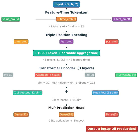
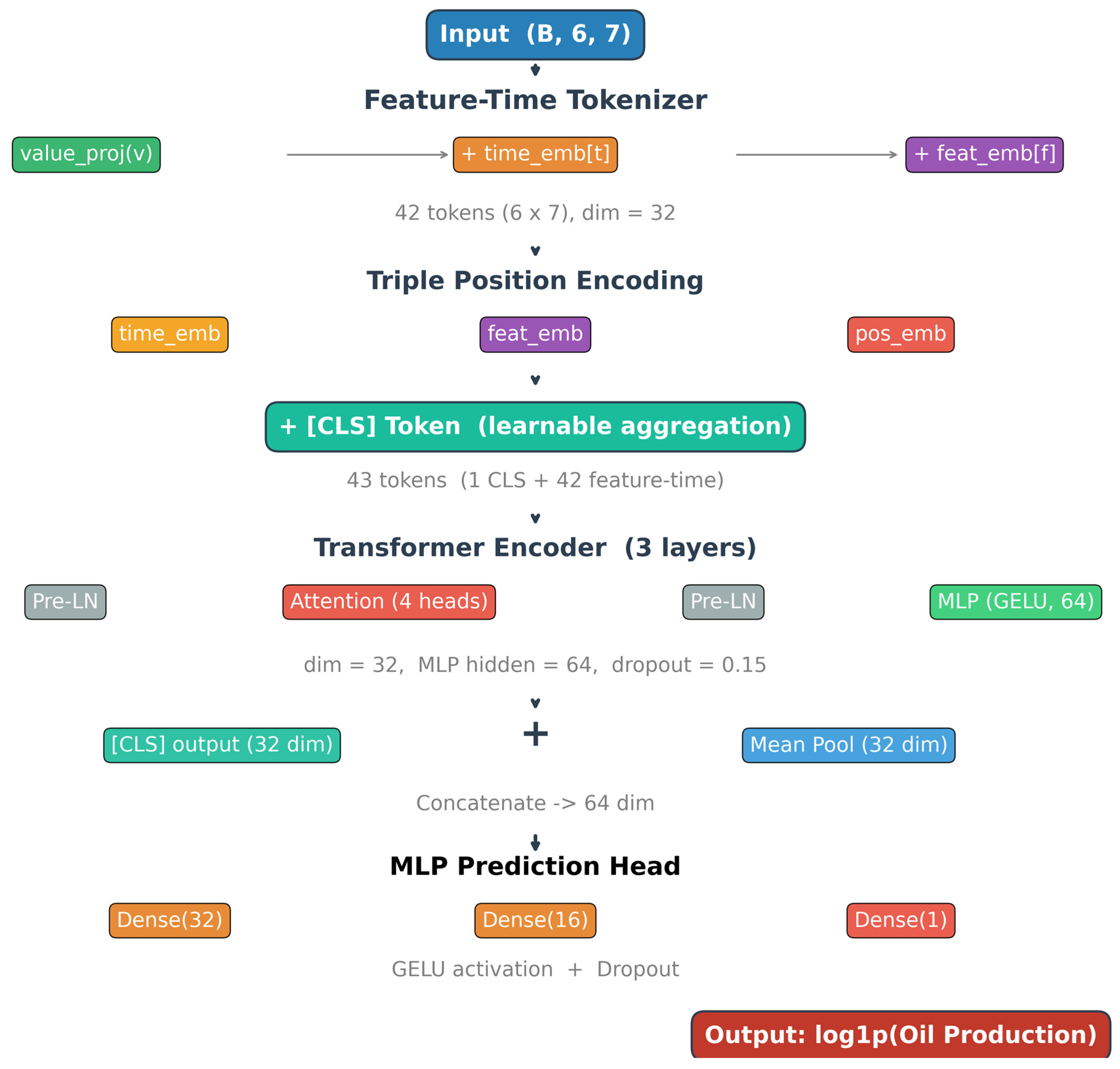
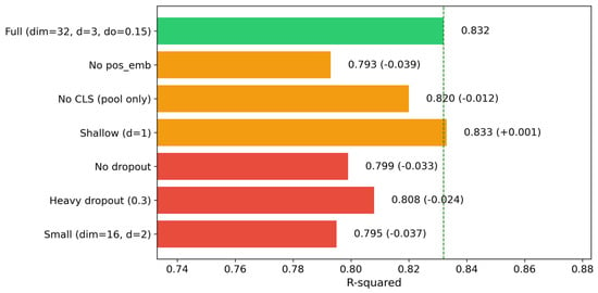
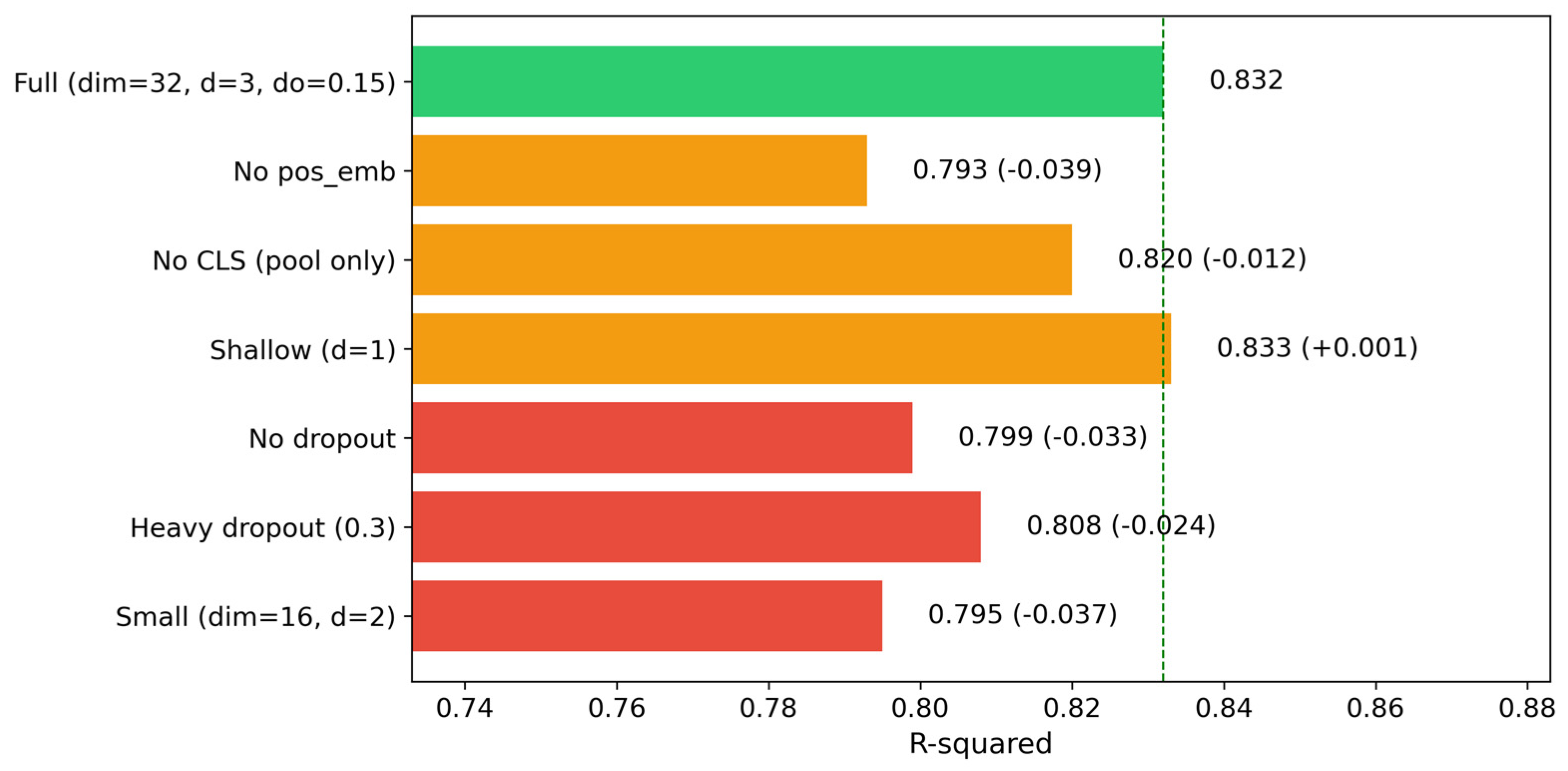
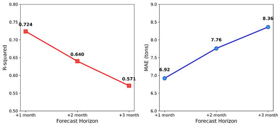
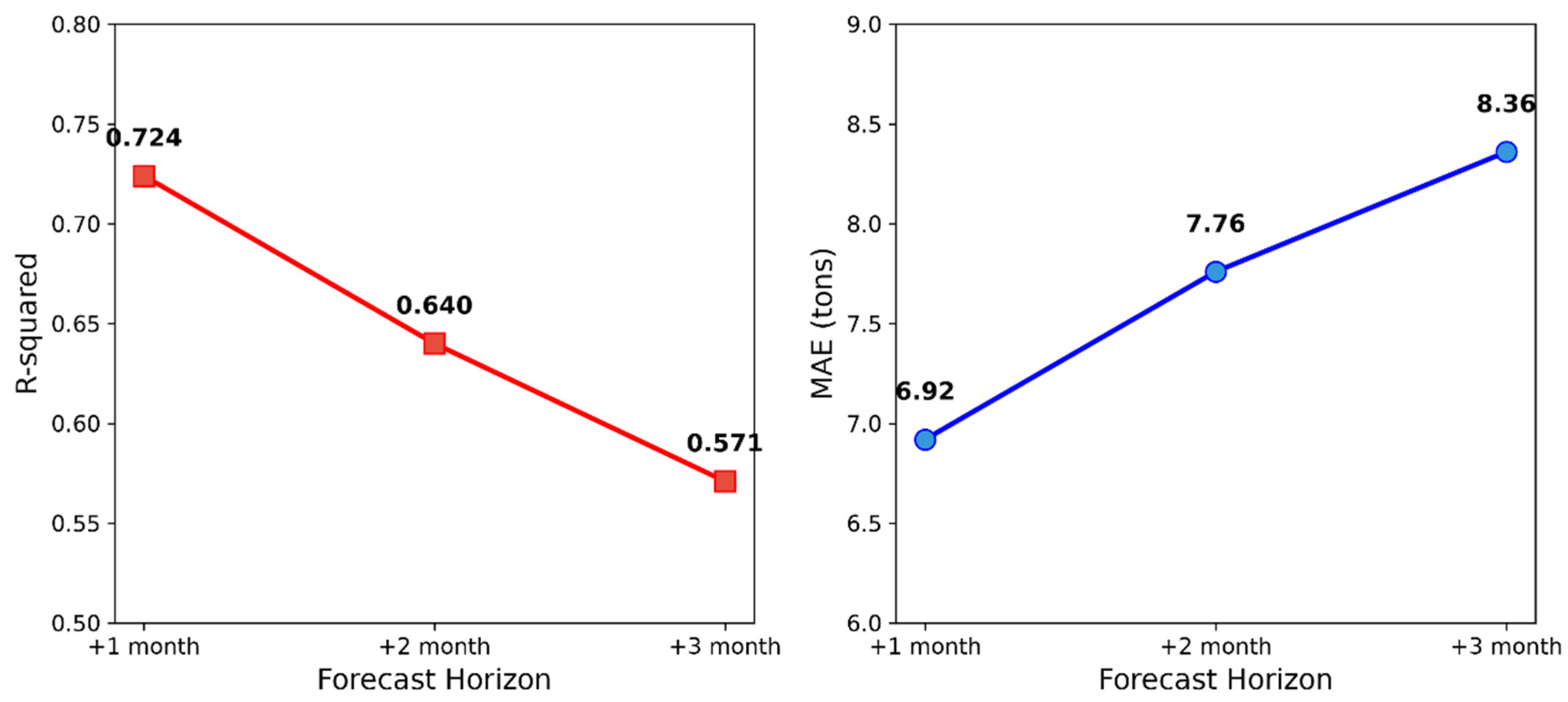
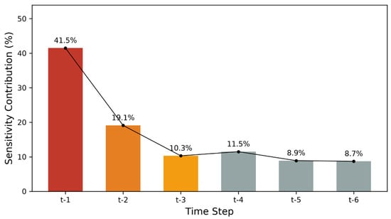
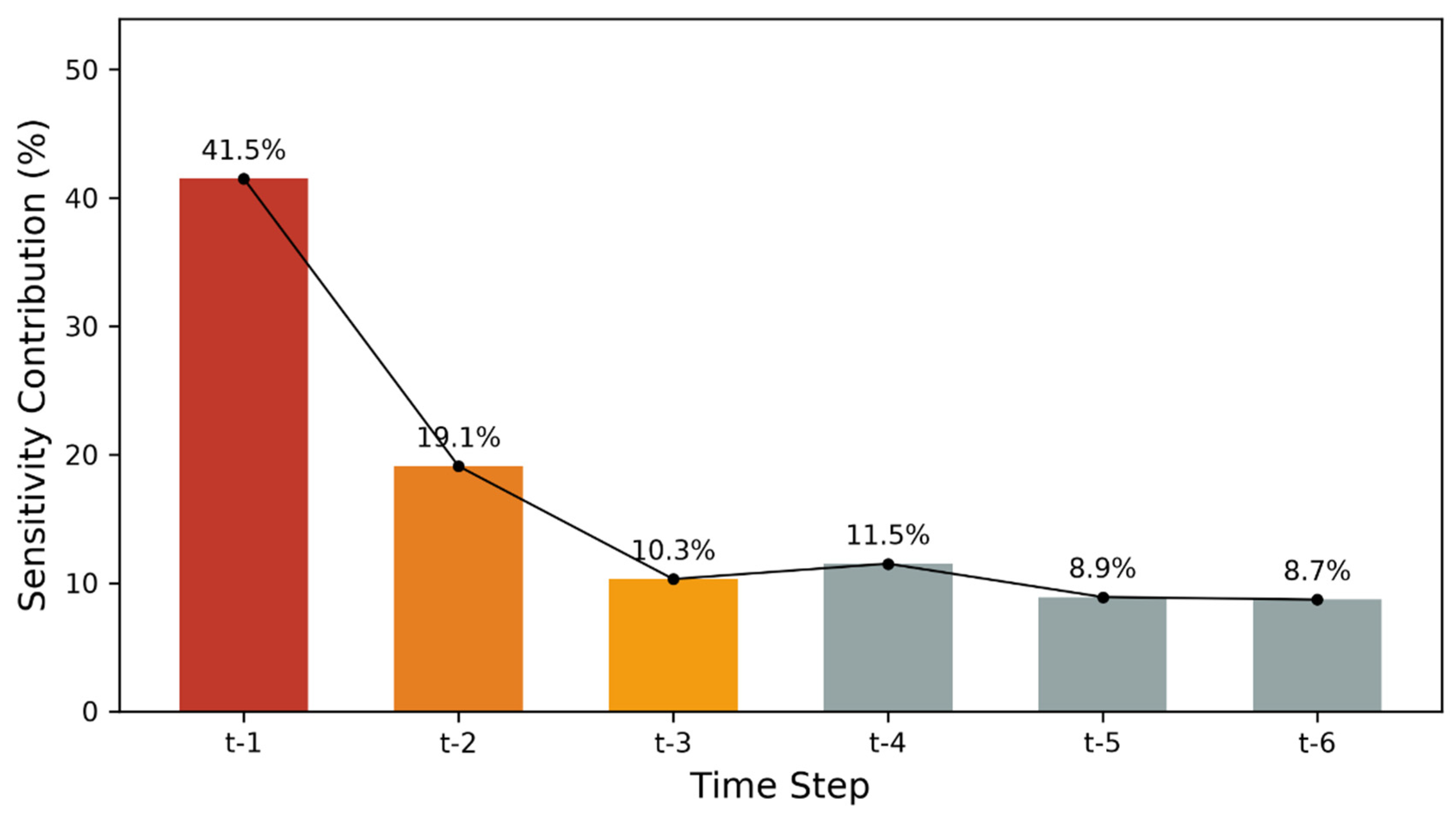
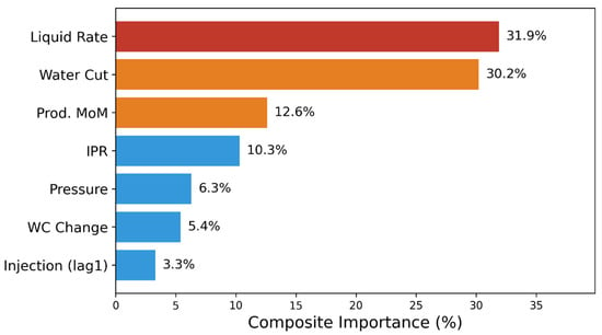
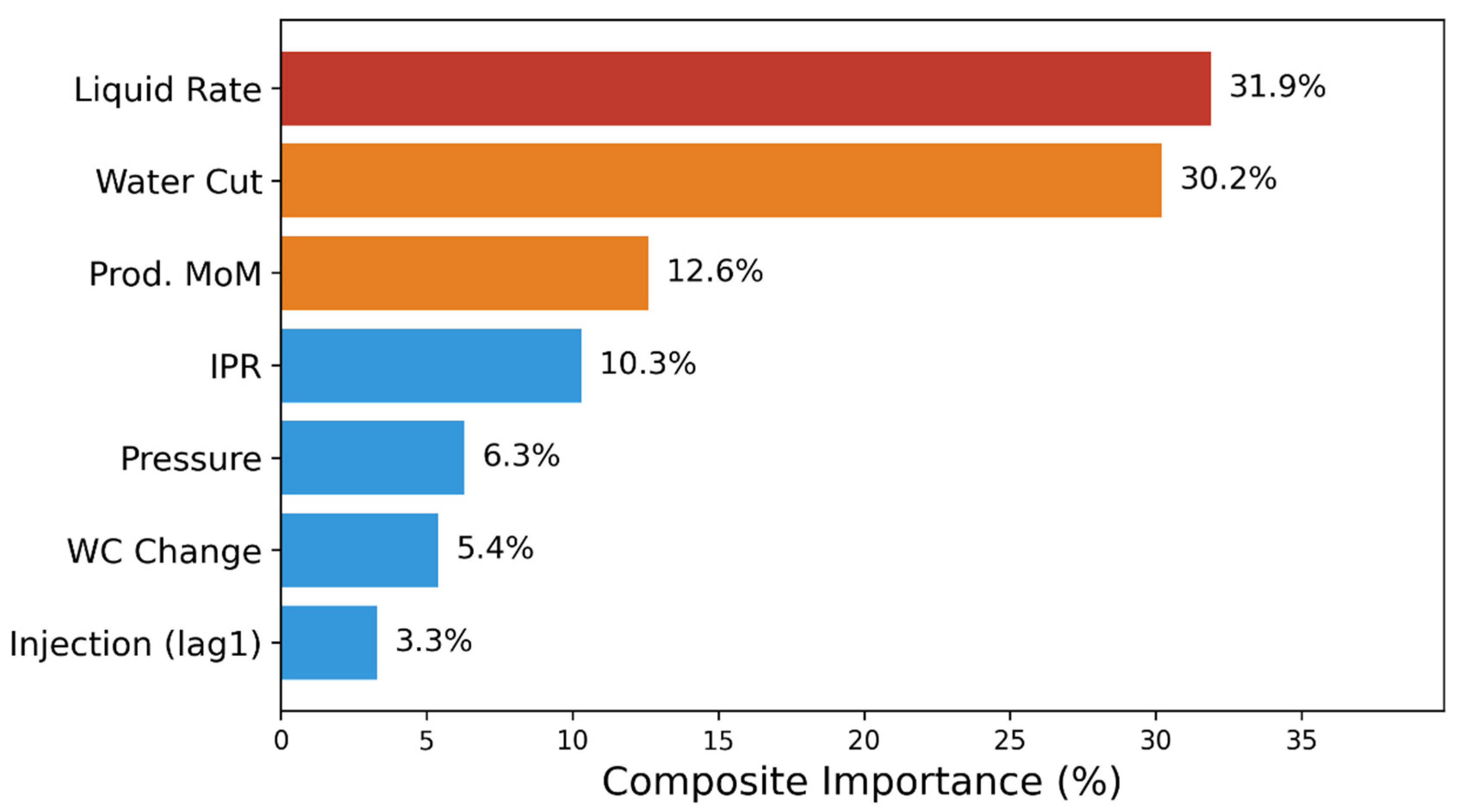
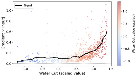
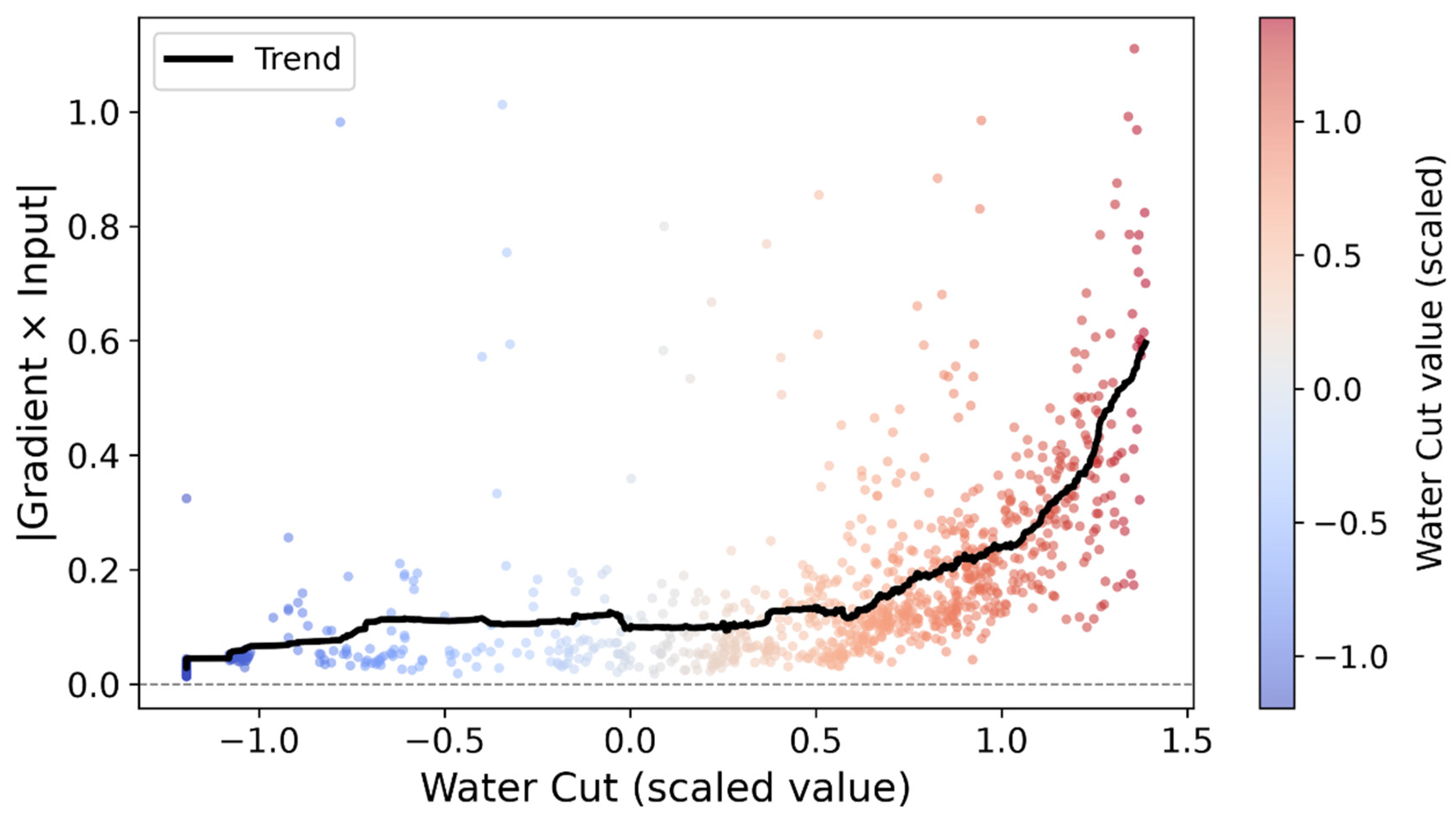
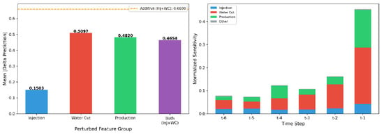
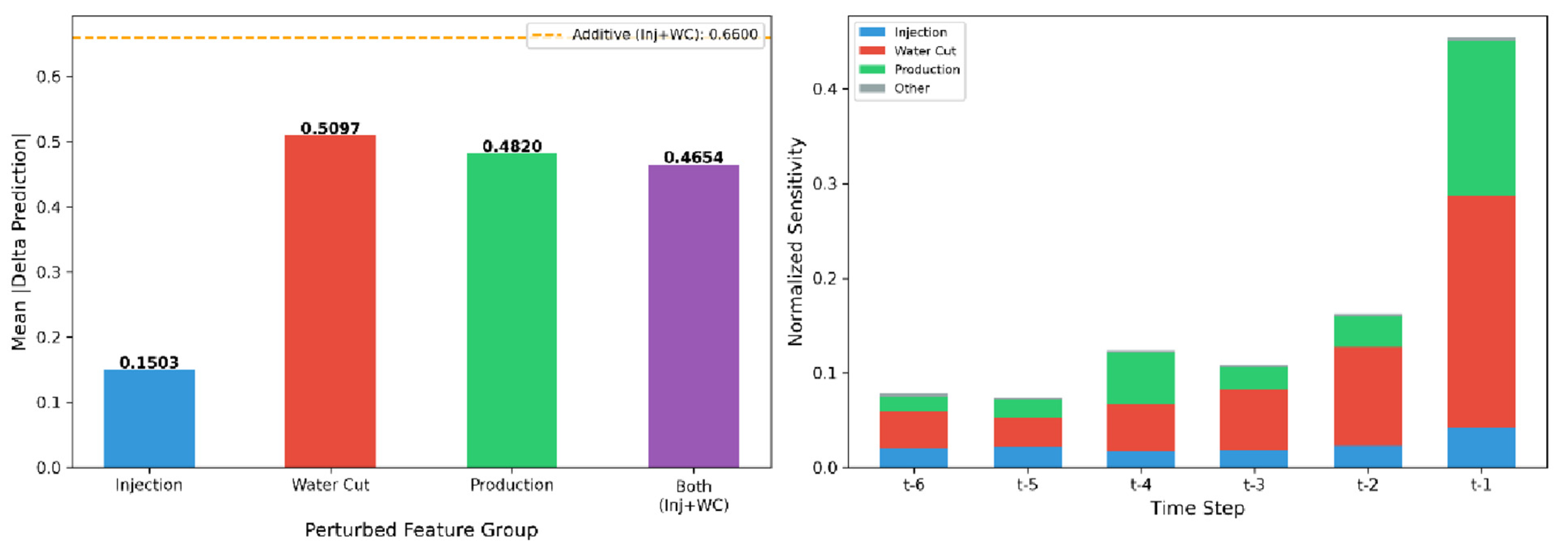

Disclaimer/Publisher’s Note: The statements, opinions and data contained in all publications are solely those of the individual author(s) and contributor(s) and not of MDPI and/or the editor(s). MDPI and/or the editor(s) disclaim responsibility for any injury to people or property resulting from any ideas, methods, instructions or products referred to in the content. |
© 2026 by the authors. Licensee MDPI, Basel, Switzerland. This article is an open access article distributed under the terms and conditions of the Creative Commons Attribution (CC BY) license.