


Abstract
High-speed railways are expanding into seismic zones, where earthquakes severely threaten the safety of vehicles on bridges. Existing seismic studies of high-speed railway bridges mainly address the structural fragility of the overall bridge, piers, and bearings. However, field observations show vehicles often derail before major bridge damage during earthquakes. Fragility analysis based on vehicle derailment as the failure criterion is urgently needed. A core task in fragility analysis of vehicle derailment is to select an optimal ground motion intensity measure (IM). In this study, the dynamic analysis of the vehicle–bridge interaction system under earthquakes was conducted using the incremental dynamic analysis (IDA) method. The characteristics of the IDA curves of the derailment coefficient and the wheel unloading were investigated. Ground motion IMs are classified into time-history-related and spectrum-related categories. The derailment coefficient and wheel unloading are adopted as engineering demand parameters (EDPs). Probabilistic seismic demand models (PSDMs) are established, and 22 candidate IMs are evaluated based on efficiency, practicality, and proficiency criteria. The results revealed that the proficiency of spectrum-related IMs is better than that of time-history-related IMs. The Sa(T1) performs the best among the 22 candidate IMs for the derailment coefficient, and ASI performs the best for the wheel unloading.
1. Introduction
High-speed railway, with large capacity and high punctuality, has become one of the core modes of transportation. As the global high-speed rail network continues to expand, the vehicle running safety and reliability are becoming increasingly prominent. However, due to geographical limitations, high-speed rail lines inevitably pass through seismically active areas; earthquakes are characterized by suddenness and destructive power, posing a serious threat to the high-speed railway system. Ensuring the vehicle’s running safety (avoiding derailment) and structural safety (preventing collapse or serious damage) of high-speed railway lines under earthquakes has become a core issue in the fields of earthquake engineering and structural engineering [1,2,3,4].
Currently, seismic research on high-speed railway bridges mainly focuses on the fragility analysis of the bridge structure itself, i.e., assessing the damage probability of key components such as piers and bearings under a given seismic intensity [5,6,7]. However, the threat of earthquakes to railway systems is not limited to the collapse of bridge structures but is more significantly manifested in the risk of vehicle derailment on the bridges [2,8]. Existing seismic damage surveys and numerical simulations show that vehicle derailment caused by earthquakes often occurs before the bridge structure suffers serious damage [9], which means that the threshold for vehicle derailment may be significantly lower than the threshold for structural damage. Seismic design based solely on the fragility of bridge structures cannot guarantee the running safety of vehicles on the bridge during an earthquake. Thus, establishing a fragility analysis method based on vehicle derailment as the failure criterion has become an urgent need [10].
Fragility analysis is used to assess the probability of damage to dynamic systems under seismic loading, and some of these include hybrid frameworks that combine artificial intelligence, computer vision [11], and probabilistic mechanics, which have been developed in recent years. One of the core tasks of fragility analysis is to select an optimal ground motion intensity measure (IM) [12]. An optimal IM can accurately predict the structural response and greatly improve the precision of the seismic fragility curve. Research on the selection of ground motion IM for bridges has been well established. Chen et al. [13] studied the influence of ground motion characteristics on the PSDM of a long-span cable-stayed bridge and pointed out that the amplitude, frequency contents, and time duration of ground motion have a significant impact on the PSDM of the bridge. Zhong et al. [14] conducted finite element analysis on a cable-stayed bridge using pulse-like near-fault ground motions. Based on a comprehensive evaluation of the near-fault seismic response and ground motion IM selection criteria, they recommend that PGA is suitable for short-period components (e.g., piers), while PGV is suitable for long-period components (e.g., towers). The optimal IM has been found to vary significantly across different bridge types and seismic contexts. For highway bridge portfolios in the Central and Eastern United States, Padgett et al. [7] compared ten candidate IMs and identified PGA as the preferred choice. In contrast, for extended pile-shaft-supported bridges in liquefiable and laterally spreading soils, Wang et al. [15] examined 26 IMs and demonstrated that velocity-related measures outperform acceleration-, displacement-, or time-related IMs in producing reliable PSDMs. Similarly, Wei et al. [16] investigated multi-pylon cable-stayed bridges with super-high piers and reported that PGV serves as the optimal IM for seismic design of this bridge type. Matsuzaki [17] investigated the optimal IM for the life-cycle seismic fragility assessment of isolated bridges. Results show that SI is optimal for the lead rubber bearings, and PGV is optimal for the columns. These findings highlight that the optimality of an IM is highly case-dependent and may not be directly transferable across different structural systems.
However, research on IMs for running safety assessment of vehicles running on bridges remains limited. The IMs commonly used in the seismic analysis of bridge structures (such as PGA, PSA, and Sa) mainly reflect the structure’s inertial forces or damage conditions and are unable to effectively characterize the effects of ground motions on the wheel–rail contact conditions [2,18]. Some scholars have carried out preliminary explorations: Luo [19] proposed a simple bridge deck vibration IM (spectral intensity, SI) to assess the running safety of vehicles on bridges under earthquakes, and it was incorporated into the Japanese standard [20] to guide the design of railway bridges. This IM is obtained by integrating the velocity response spectrum of deck acceleration during earthquakes based on the vehicle–bridge decoupling method from 0.1 s to 2.5 s. By limiting bridge deck vibration (limiting SI value), the running safety of vehicles on bridges during earthquakes can be ensured. Jin and Liu [21] adopted a vehicle–bridge decoupling approach and used the relative wheel–rail displacement as a derailment criterion. They analyzed the correlation between IMs of the bridge deck vibration and the wheel lift and subsequently developed the derailment fragility cloud map to evaluate the vehicle safety on bridges during earthquakes. Liu et al. [22] evaluated the correlation between some IMs and vehicle running safety and found that velocity spectral intensity (VSI) and Housner intensity (HI) have good correlations for a wide range of structural periods, and recommended them as optimal IMs for safety analysis of vehicles running on bridges during earthquakes. Although some work was done on selecting optimal IMs to assess the safety of vehicles running on bridges during earthquakes, the PSDM relationship between these IMs and derailment indexes has not yet been systematically established. The applicability of different IMs for assessing the safety of vehicles is not yet sufficient.
In this study, the PSDM based on the classical Cornell formulation was adopted for the vehicle–bridge interaction (VBI) system, and the applicability of this modeling framework to vehicle–bridge coupling problems was examined. Dynamic analysis of the vehicle–bridge interaction (VBI) system during earthquakes based on the IDA method was conducted. The ground motion IMs are classified into two categories: time-history-related and spectrum-related IMs. Taking the derailment coefficient and wheel unloading as the engineering demand parameters (EDPs), probabilistic seismic demand models (PSDMs) are established. Based on the selection criteria of efficiency, practicality, and proficiency for IMs, the optimal IMs for evaluating the running safety of vehicles on bridges during earthquakes were identified.
2. Probabilistic Seismic Demand Models and Optimal IM Selection Criteria
2.1. Probabilistic Seismic Demand Model
The PSDM is a core component in performance-based seismic design for structural engineering [23]. Its function is to establish a statistical relationship between the IMs and the EDP, quantify the probability that a structure will reach the specific damage state under a given seismic intensity, and provide key support for the construction of seismic fragility curves. The PSDM was proposed by Cornell et al. [24] in the dynamic analysis of building frames. This method assumes that the seismic response EDP is a random variable that follows a log-normal distribution [25]. Therefore, under a given ground motion IM, the probability that the structural EDP exceeds a certain damage state limit d can be written as
where is the standard normal cumulative distribution function; represents the median of the structural EDP; It is assumed that the relationship between the median structural EDP and the ground motion IM is
where the parameters a and b are the corresponding estimated parameters obtained using the least squares method.
Equation (2) can be written in an equivalent logarithmic form as
The relationship between IM and EDP is assumed to follow a linear form in logarithmic space established by Equation (3). ln(a) and b are the vertical intercept and slope, respectively, obtained from the least squares method. The dispersion of the EDP prediction is quantified by the logarithmic standard deviation . Generally, is related to the value of IM. In PSDM analysis, is assumed to be a constant and is calculated by the following formula:
where represents the extreme value of the response under the i-th earthquake; n represents the number of ground motion records.
2.2. Optimal IM Selection Criteria
The use of the optimal IM enables a more accurate assessment of the running safety of vehicles on bridges during earthquakes [26]. In the PSDM, the optimal IM is selected based on the selection criteria suggested in references [7,26,27,28]. In this study, three different criteria (efficiency, practicality, and proficiency) were examined to determine the optimal IMs for the VBI dynamic system. The candidate IM that consistently performs best across all three criteria is selected as the optimal IM.
- (1)
- Efficiency: It directly reflects the uncertainty of the EDP of the structural dynamic system under a given IM. The efficiency of the IM can be quantified by the logarithmic standard deviation (see Equation (4)) from the linear regression of EDP against IM in log-space. When IM is given, the lower the dispersion of the structural response, the more accurately the EDP can be predicted. Furthermore, under the same accuracy requirements, an efficient IM can significantly reduce the number of ground motion records required for analysis and the computational cost of nonlinear dynamic time history analysis. Efficiency is measured by the dispersion of the linear regression between the EDP and the ground motion IM in logarithmic space [29]. A smaller dispersion value indicates higher efficiency of the ground motion IM.
- (2)
- Practicality: This is an indicator that measures whether there is a direct correlation between the EDP and the ground motion IM of the dynamic system [30]. It measures the sensitivity of the EDP to changes in the IM, reflecting the dependence of the EDP on changes in the IM. The stronger the dependence of the EDP on the IM, the more significant the change in EDP caused by a small change in IM. Practicality is quantitatively characterized by the linear regression slope b in the PSDM (see Equation (3)). A larger value of b indicates that the IM has good practicality.
- (3)
- Proficiency: This is an indicator that comprehensively considers efficiency and practicality, aiming to balance the accuracy of prediction and the sensitivity to changes in IM. It avoids the bias in evaluation results caused by using efficiency or practicality alone. Substituting Equation (3) into Equation (1) gives
In terms of proficiency, IMs with lower are preferred, as they combine stronger correlation with the EDPs and lower prediction dispersion.
3. Vehicle–Bridge Interaction Model and EDPs
3.1. Vehicle–Track Model
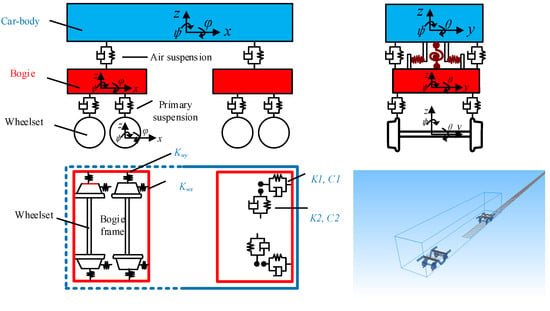
The vehicle system is established within the framework of multi-rigid-body dynamics. Each vehicle comprises seven rigid bodies: one car body, two bogies, and four wheelsets. All components are treated as rigid bodies, neglecting elastic deformation. The longitudinal DOFs are omitted under the assumption of constant vehicle speed. Consequently, each car body and bogie possesses five DOFs. Given constant rotational speed, the wheelset pitch is neglected, leaving four DOFs per wheelset. The four-axle vehicle is simplified as a dynamic model with 31 degrees of freedom.
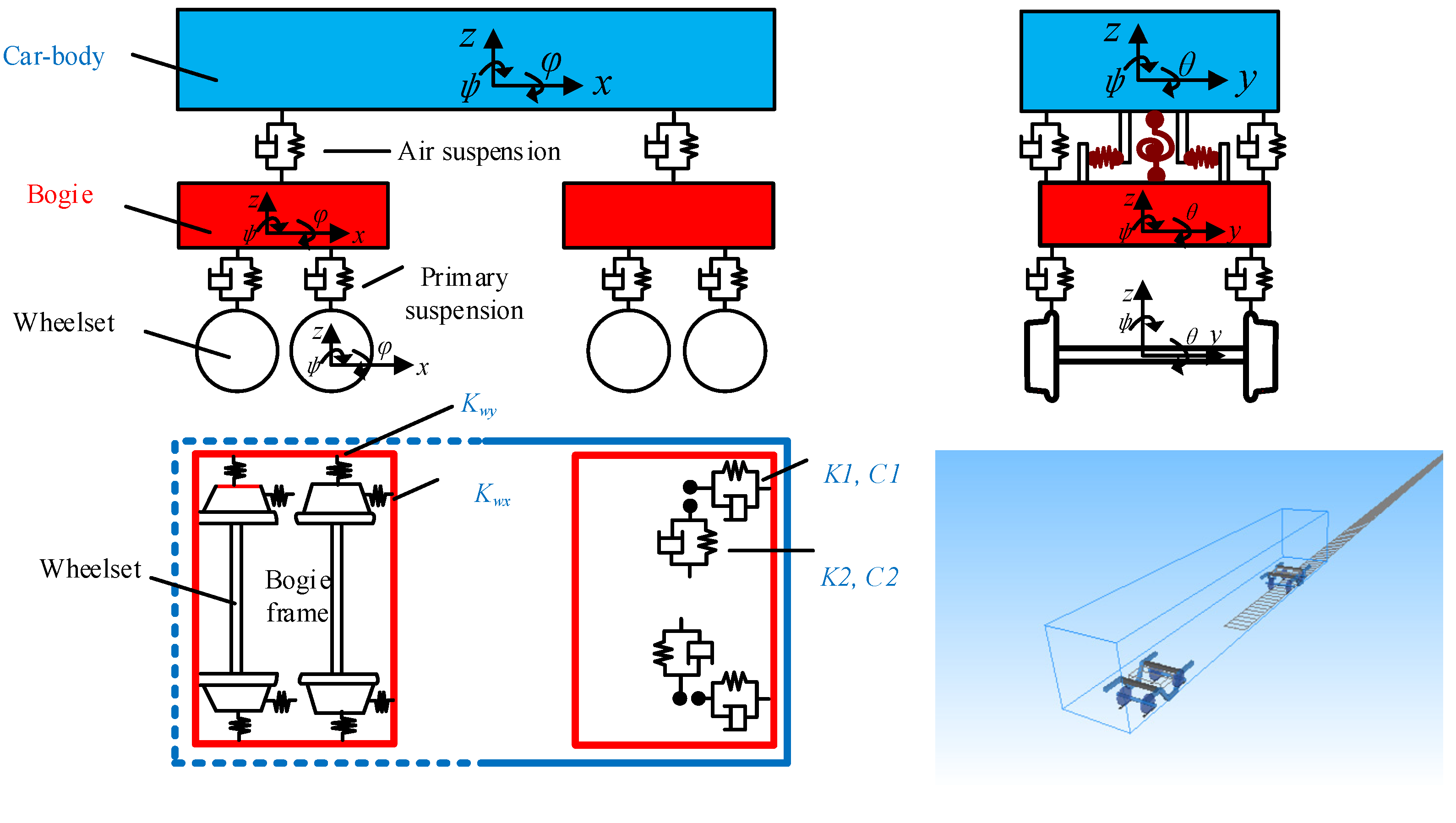
Each component of the vehicle system is simplified as being connected by spring-damping elements. The car body is connected to two bogies through a secondary suspension, and the bogies are connected to the wheelsets through a primary suspension. The secondary suspension consists of four sets of three-dimensional spring-damping elements, and the primary suspension consists of eight sets of three-dimensional spring-damping elements. A simplified diagram of the vehicle dynamics model of the high-speed railway vehicle is shown in Figure 1. The values of the vehicle’s suspension parameters and spatial parameters are from Ref. [31].
Figure 1.
Schematic diagram of a typical vehicle model.
The dynamic equation of the vehicle system can be written as
where , , and are the mass, damping matrix, and stiffness matrix of the vehicle, and , , and are the displacement, velocity, and acceleration vectors.
The rail is simulated using an elastic beam, and its vibration includes two degrees of freedom: lateral and vertical. The fastening system is simulated as a linear spring-damped element, connecting the rail nodes to the track slab nodes and providing both lateral and vertical stiffness. The motion equations of the rail can be written as
where , , and are the mass, damping matrix, and stiffness matrix of the rail, respectively, and , and are the displacement, velocity, and acceleration vectors, respectively. is the force vector acting on the rail from the vehicle, and is the force vector acting on the rail from the bridges. The vector is used to apply seismic force on the DOFs of the track structure. If the DOF of the track structure represents the lateral direction, the element of is equal to 1; otherwise, the element of is set to 0. is the acceleration of the ground motion.
The nonlinear wheel–rail contact model consists of three parts: wheel–rail geometric contact problem, wheel–rail normal force, and wheel–rail tangential force. In this study, the trace curve method [32] is used to find the contact point between wheel and rail. The wheel–rail normal force was calculated using the Hertz nonlinear contact theory [33]; and the frictional force in the tangential direction is calculated using the Shen–Hedrick formula [34].
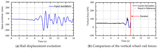
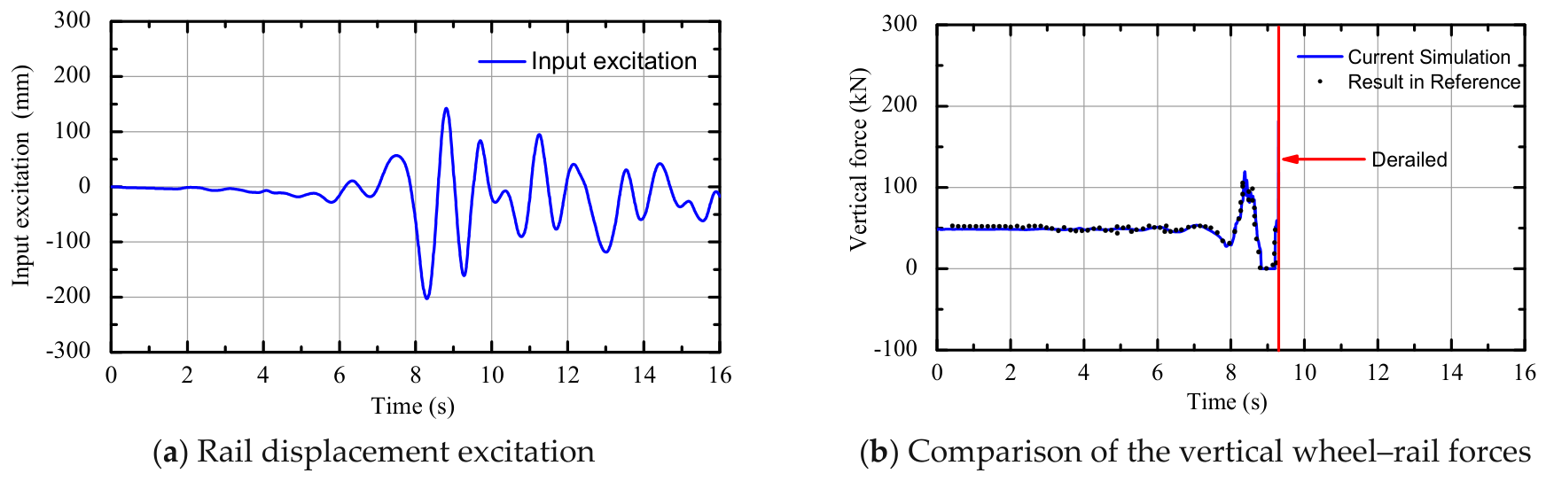
To verify the accuracy of the vehicle–track model, the track vibration excitation from Ref. [9] was input into the vehicle–track system, and the calculated result in the present study was compared with that in Ref. [9]. Figure 2a shows the input track displacement excitation from the literature, and Figure 2b shows the comparison of wheel–rail forces. The blue solid line in the figure represents the simulation results in this study, and the black dots represent the results from Ref. [9]. It can be seen that the simulation results match the results in the literature well, proving the accuracy of the model.
Figure 2.
Verification of the current simulation.
3.2. Bridge Models
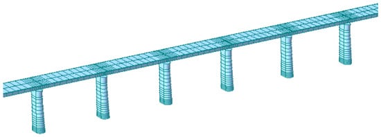
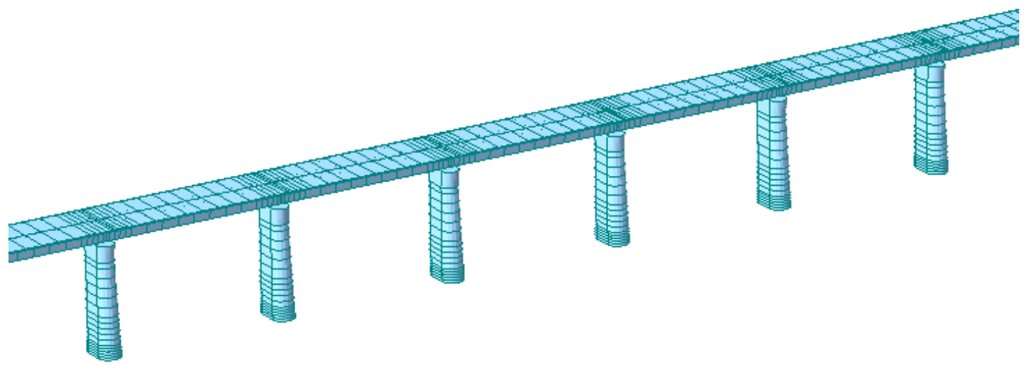
In this study, the running safety of a vehicle crossing a series of simply supported bridges under earthquakes was examined. The bridges were modeled using the finite element method (FEM), as illustrated in Figure 3. Both the beams and piers were modeled by 3D beam elements, each containing two nodes with six degrees of freedom: three translations and three rotations. The bridge span was set to 32 m with a box-section beam that is commonly adopted in China’s high-speed railway systems. The bridge is composed of 50 spans with a total length of 1600 m. For simplicity of the bridge model, the heights of the piers were kept constant, which was chosen as 23 m. The main girder in each span is divided into 18 elements, while each pier is modeled with 17 elements. Mesh refinement is implemented at the span-to-span connections of the girder and at the pier bases. The piers feature a variable cross-section along their height. The sectional properties of beams and piers are from Ref. [35] and are shown in Table 1. The main girders are constructed with C50 concrete, while the piers are made of C35 concrete. The secondary dead loads of the bridge are considered in the material density of the beam. A simply supported boundary condition at both ends of the bridge girder is considered in this study, with the left end constrained in the longitudinal, transverse, and vertical translations, and the right end constrained in the transverse and vertical translations while allowing longitudinal displacement. The pier bottoms are fixed at the foundation level (all translational and rotational degrees of freedom are restrained). The bearings are modeled as elastic connection elements with specified stiffnesses in the longitudinal, transverse, and vertical directions.
Figure 3.
Finite element model of bridge.
Table 1.
Sectional properties of the bridge.
The connection between the rail and the bridge is simplified to a linear spring and damping connection. The interaction force between the bridge and the rail can be obtained from their relative displacement and velocity, as shown in the following formula:
where represents the lateral force between the bridge and rail; represents the vertical force between the bridge and rail; and represent the lateral stiffness and damping, respectively; and represent the vertical stiffness and damping of the vertical constraint, respectively; and represent the lateral and vertical displacements of the rail, respectively; is the lateral distance between the rail and the centroid of the main beam; , and represent the lateral displacement, vertical displacement, and angular displacement of the centroid of the main beam, respectively; is the height from the centroid of the main beam to the bottom of the rail.
The initial conditions of the VBI system are set as follows: the gravitational loads of the vehicle are applied as static loads before the seismic excitation begins, and the initial equilibrium state of the vehicle–bridge system is determined through static analysis. The dynamic equation of the bridge structure is
where Mb, Cb, and Kb are mass, damping, and stiffness matrices of the bridge dynamic system, respectively. is the force vector from the rail. Regarding the system’s damping, the Rayleigh damping matrix is used in this study:
where and are Rayleigh damping coefficients. The Rayleigh damping coefficients can be calculated as
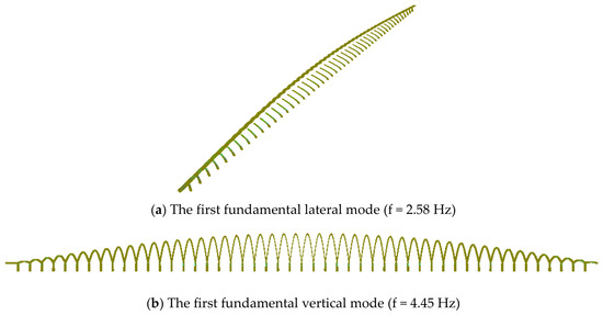
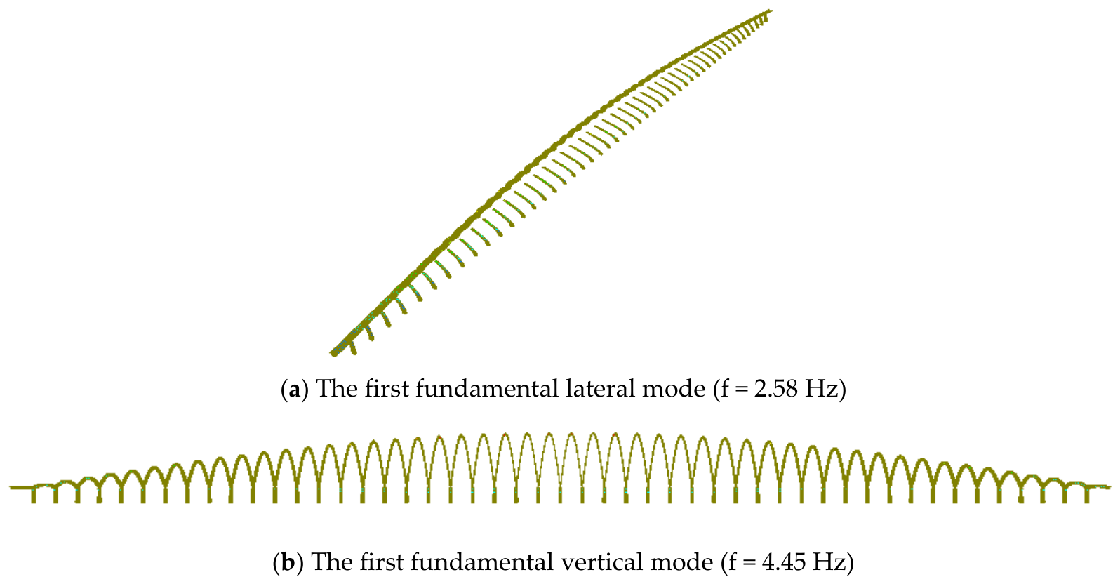
where and are the natural angular frequencies of two selected vibration modes. The damping ratio , which is determined by the materials, is chosen as 0.05 in this study. Figure 4 illustrates the modal shapes for both lateral and vertical vibrations. The corresponding fundamental frequencies are 2.58 Hz (lateral) and 4.45 Hz (vertical). The direct integration method (Newmark-β) was used to solve the dynamic response of the bridge system. The two dominant modal frequencies are adopted to determine the Rayleigh damping coefficients (α and β) for constructing the structural damping matrix, which are essential for the time-history analysis of the bridge dynamic system.
Figure 4.
Bridge modes and natural frequencies.
3.3. Derailment Criteria and Engineering Demand Parameters
The EDP is a measure for quantifying the structural seismic response. For the VBI system, two commonly used EDPs for evaluating vehicle running safety were adopted in this study. They provide a comprehensive assessment of running safety from both lateral and vertical perspectives: the derailment coefficient quantifies the lateral stability of the wheel–rail contact; the wheel unloading captures the risk of overturning or a decrease in vertical force. The derailment coefficient and the wheel unloading are denoted as EDP1 and EDP2, respectively.
The derailment coefficient is defined as the ratio of the lateral force Q acting on the wheel to the vertical force P. It was used to quantify the tendency of the wheel flange to climb along the rail head due to the lateral force. The critical value of this index is derived from a theoretical model established by Nadal based on static equilibrium conditions. When the derailment coefficient exceeds a critical threshold, the wheel flange is highly prone to climb along the side of the rail head, thus triggering geometric derailment.
The threshold of derailment coefficient differs among national standards [36,37]: the International Union of Railways (UIC) adopts 1.2, while 0.8 is used for German ICE trains and Chinese high-speed railways. Experiments and simulations show that during earthquakes, the derailment coefficient of a vehicle running on bridges can momentarily exceed the safety limit. Shaking table tests reveal that even when the instantaneous coefficient reaches twice the limit, actual derailment does not occur, suggesting a safety margin in current standards under seismic conditions. Although there is no specific threshold for the derailment coefficient under seismic conditions, it remains an important indicator for assessing the safety of vehicles on bridges during earthquakes.
Wheel unloading is defined as the ratio of the reduction in wheel–rail vertical force ΔP to the static wheel load P0. It is used to evaluate the risk of wheel derailment due to a sharp decrease in vertical force, which may lead to the wheel detaching from the rail surface.
The limit values for wheel unloading differ among countries. In China, the limit is set at 0.8. Some other countries have specified limits for dynamic wheel unloading. Germany and the United States adopt a limit of 0.9, and Japan adopts a limit of 0.8. The Ref. [36] shows that even when the wheel unloading reached 1 under certain operating conditions, the vehicle did not derail. Under seismic excitation, the wheel unloading is a relatively conservative derailment criterion. Namely, the threshold may overestimate the actual derailment risk. Despite this conservatism, it still holds engineering value as an early risk warning indicator, capable of identifying potential derailment trends.
4. Ground Motion Selection and Intensity Measures
4.1. Selection of Ground Motion Records
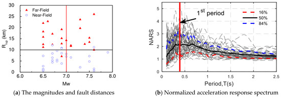
The strong randomness of ground motion means that a single or a small number of ground motion samples cannot cover the uncertainties in amplitude, spectrum, and time duration. To cover a wide range of uncertainties in ground motions, this study introduces a set of 50 ground motion records (22 far-field and 28 near-field sets) recommended by FEMA P695 as excitation inputs [38]. The magnitudes and fault distances are shown in Figure 5a. This ground motion set contains far-field, near-field non-pulse and near-field pulse ground motions, systematically covering the characteristics of strong ground motions under different fault distances, magnitudes, and site conditions.
Figure 5.
The selected ground motion characteristics.
Figure 5b shows the normalized Acceleration Response Spectrum (NARS) and statistical characteristics for all selected ground motions. The NARS are obtained from the acceleration response spectra divided by the peak acceleration of the ground motion. The solid black line in the figure represents the mean of the response spectrum, while the red and blue dashed lines correspond to the 16th and 84th percentile spectra, respectively. These visually reflect the dispersion among the ground motion records. The red vertical solid line in the figure represents the first-order period of the bridge structure. As can be seen from the figure, at the bridge’s fundamental period T1 = 0.39, the mean peak amplification factor of the ground motion reaches 2.1. Furthermore, near the bridge’s first-order fundamental period, the 16th–84th percentile range (i.e., the 68% confidence interval) is quite wide. The representativeness and comprehensiveness of the selected ground motions in terms of spectral shape can provide sufficiently stringent and diverse input conditions for the seismic assessment of vehicle running safety on bridges. This helps avoid overly optimistic analysis results that may arise from overly homogeneous selection of ground motion records.
4.2. Candidate Ground Motion Intensity Measures
Intensity measures (IMs), as parameters for quantifying the potential destructive power of ground motions, are core input variables in structural seismic design and performance assessment. There are significant differences in the effectiveness of different IMs in predicting the seismic response of vehicles. Therefore, selecting the optimal IM with a good correlation to EDPs of the VBI system is of significant research importance.
The optimal ground motion IM should comprehensively reflect characteristics of amplitude, spectrum, and time duration. Taking into account the three factors above, 22 IMs commonly used in engineering are selected in this study as a candidate IM library. These IMs are divided into two categories: (1) time-history-related IMs, such as PGA, PGV, PGD, etc.; (2) spectrum-related IMs, such as PSA, PSV, PSD, etc. The specific definitions of the candidate IMs are shown in Table 2.
Table 2.
Candidate ground motion IMs.
5. Incremental Dynamic Analysis of Vehicle–Bridge Interaction System
5.1. IDA Procedure
The IDA method is adopted to prepare the IM-EDP data for the construction of PSDM. IDA performs nonlinear time-history analysis on the VBI system by incrementally scaling the ground motion IM (e.g., PGA) across multiple ground motion records. When applied to the running safety assessment of vehicles on bridges during earthquakes, IDA offers two key advantages. (1) It can characterize the dynamic response characteristics of vehicles on the bridge under different ground motion intensity levels, such as the development process and limit state of the derailment coefficient and wheel unloading. (2) By selecting multiple representative ground motion records for IDA, it is possible to examine the effect of ground motion uncertainties on the vehicle response.
Using the IDA method, the EDP values of the vehicle under different intensity levels of ground motion are obtained for each ground motion record. The specific steps of IDA are as follows: (1) scaling of the ground motions is done such that the vehicle will reach the derailment state under earthquakes. In the IDA, each ground motion is scaled from 0.025 g to 0.7 g. (2) Then, for each earthquake intensity increment, the time history analyses are performed for the VBI system, and the vehicle seismic response is monitored. (3) IDA curves were plotted with the ground motion IM, such as peak ground acceleration (PGA), on the x-axis and derailment indicators, such as the derailment coefficient and wheel unloading, on the y-axis.
5.2. IDA of the EDPs
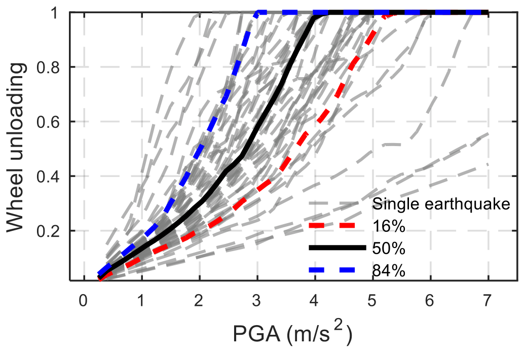
Given that the IDA curve contains a large amount of data and that there are differences between each curve, it is necessary to quantify this randomness. The IDA data are statistically analyzed assuming a log-normal distribution. For each IM intensity, the EDP mean and standard deviation are evaluated, and the response distribution is characterized by the 16%, 50%, and 84% quantile curves.
- (1)
- Derailment coefficient
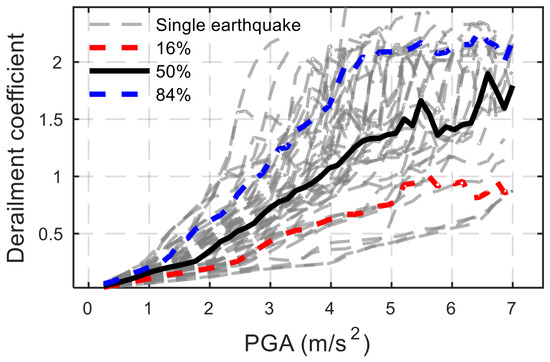
Figure 6 shows the IDA curves of the derailment coefficient for each ground motion. As can be seen from the figure, in the initial stage (PGA < 1.75 m/s2), the IDA curve of the vehicle derailment coefficient shows a linear upward trend with very little dispersion. When PGA exceeds 1.75 m/s2, the slope of the curve increases, indicating a certain degree of nonlinearity in the VBI system during earthquakes.
Figure 6.
Derailment coefficient IDA curves.
Furthermore, it is observed that as PGA continues to increase, the IDA curves display a hysteresis phenomenon. That is, with the increase in ground motion PGA, some IDA curves no longer increase monotonically at certain points but instead exhibit characteristics such as fluctuations and hysteresis. This may be due to the following reasons: when the PGA exceeds a certain threshold, the vehicle system will experience a large-amplitude response, and nonlinear behaviors such as lateral sliding or wheel–flange contact may occur between the wheel and rail. This causes the lateral and vertical forces to change asynchronously, resulting in fluctuations and hysteresis in the IDA curve of the derailment coefficient.
When PGA = 4 m/s2, the mean derailment coefficient is close to 1.1. Additionally, the width between the 16th and 84th percentiles of the derailment coefficient gradually widens with increasing PGA, reflecting uncertainty and dispersion in the VBI system response under extreme seismic conditions.
- (2)
- Wheel unloading
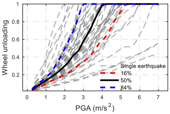
Figure 7 shows the IDA curves for the wheel unloading for each ground motion. As can be seen from the figure, in the initial stage (PGA < 1.5 m/s2), the IDA curve for the wheel unloading shows a linear upward trend with very little dispersion, indicating that the wheel and rail are still in close contact, and the entire VBI system is still approximately a linear system. At this stage, different ground motion records have little effect on the running safety evaluation of the vehicle during earthquakes.
Figure 7.
Wheel unloading IDA curves.
As the seismic ground motion intensity increases, the slope of the IDA curve for the wheel unloading increases, indicating a certain degree of nonlinearity. It can be seen that the hysteresis phenomenon of the wheel unloading IDA curve is less pronounced compared to that of the derailment coefficient. This may be due to the following reasons: the derailment coefficient involves both the lateral and vertical forces between the wheel and rail. Under strong earthquakes, nonlinear behaviors such as lateral slipping and wheel–flange contact are prone to occur between the wheel and rail. In contrast, the wheel unloading only reflects the relative unloading degree of the vertical force, and its nonlinear response trigger threshold is higher.
The median IDA curve of the wheel unloading shows that for most ground motions, the corresponding PGA value is around 2.75 m/s2 when the wheel unloading is 0.5, and around 3.5 m/s2 when the wheel unloading is 0.8. Furthermore, as the PGA of the ground motion increases, the dispersion of the IDA curve also shows a gradually increasing trend. During this stage, there are significant differences between different IDA curves, indicating that the wheel unloading of vehicles on the bridge during an earthquake is closely related to the characteristics of the input ground motion.
6. Optimal IMs Analysis
6.1. PSDM of Vehicle–Bridge Interaction System
The PSDM establishes a relationship between vehicle response peaks (derailment coefficient and wheel unloading) and ground motion IMs. It is key to quantifying the probabilistic relationship between engineering demand parameters (EDPs) and seismic motion intensity measures (IMs). The PSDM is developed using two EDPs (derailment coefficient and wheel unloading) and 22 candidate IMs for the VBI model. A linear regression is performed using the engineering demand parameter ln(EDP) against the ground motion intensity measure ln(IM), with data points obtained through time-history dynamic analysis of the VBI system under 50 ground motions. It should be noted that an IDA of the VBI system with amplitude adjustment is performed for each ground motion.
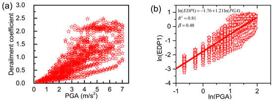
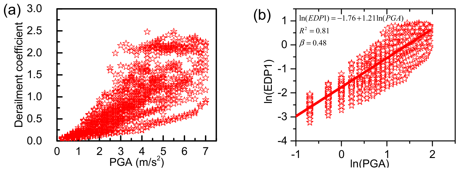
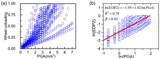
Figure 8 and Figure 9 present the results of PSDM analyses using the derailment coefficient and wheel unloading as EDPs, and Peak Ground Acceleration (PGA) as the ground motion IM. The data are presented in arithmetic and logarithmic coordinate systems, respectively. Figure 8a and Figure 9a show the data plotted in an arithmetic coordinate system, and Figure 8b and Figure 9b show the data presented in a logarithmic coordinate system.
Figure 8.
Results of derailment coefficient in (a) arithmetic scale and (b) logarithmic scale.
Figure 9.
Results of wheel unloading in (a) arithmetic scale and (b) logarithmic scale.
It can be seen from Figure 8 and Figure 9 that, with regard to the EDPs (derailment coefficient and wheel unloading), in the arithmetic coordinate system, the relationship between the engineering demand parameters and the ground motion IM exhibits a power-law curve (consistent with the assumptions in Section 2.1). Applying a logarithmic transformation linearizes the relationship, thereby greatly improving analytical efficiency and model feasibility.
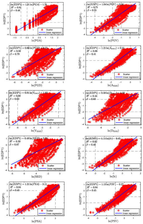
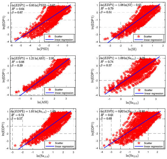
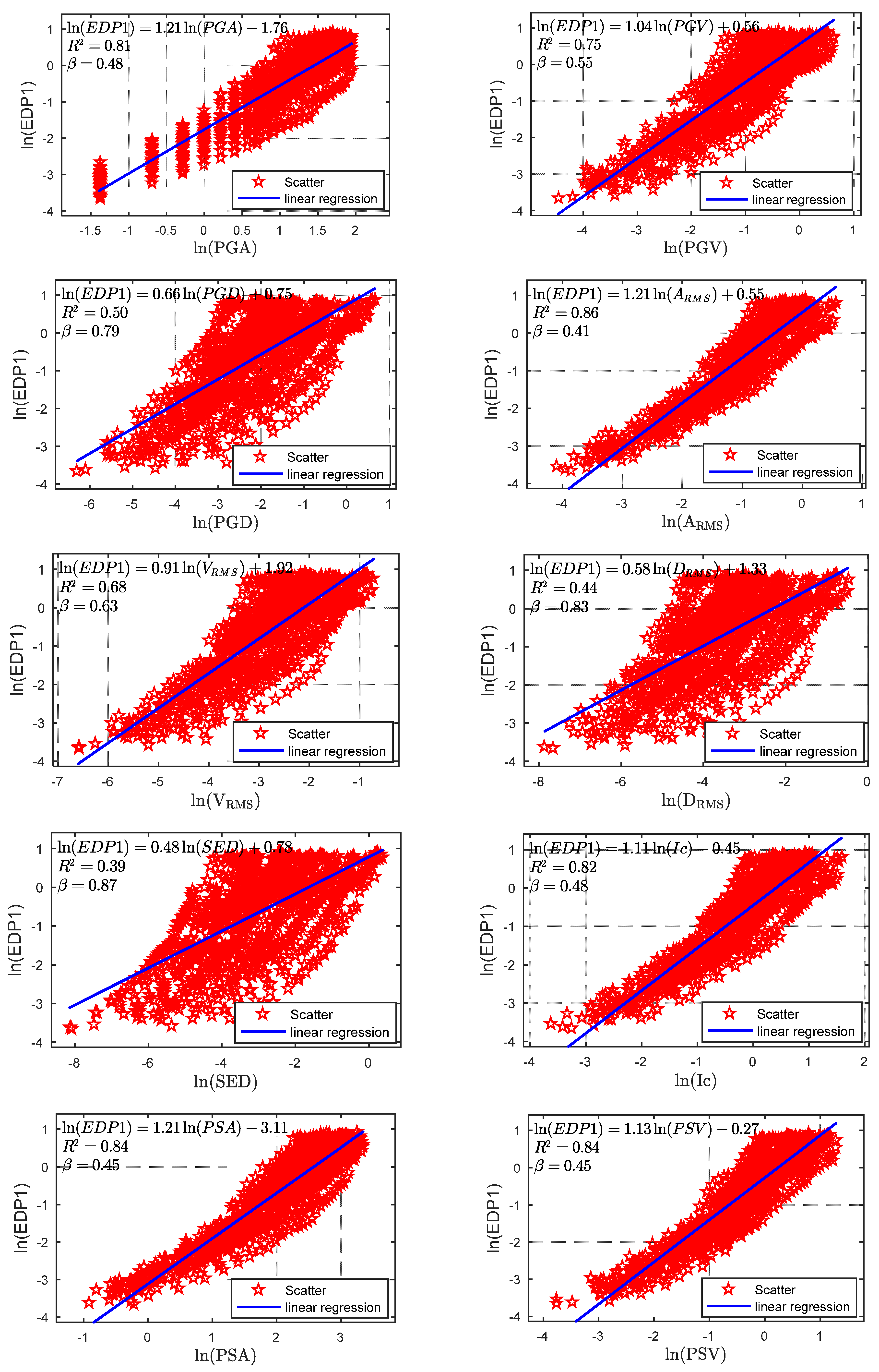
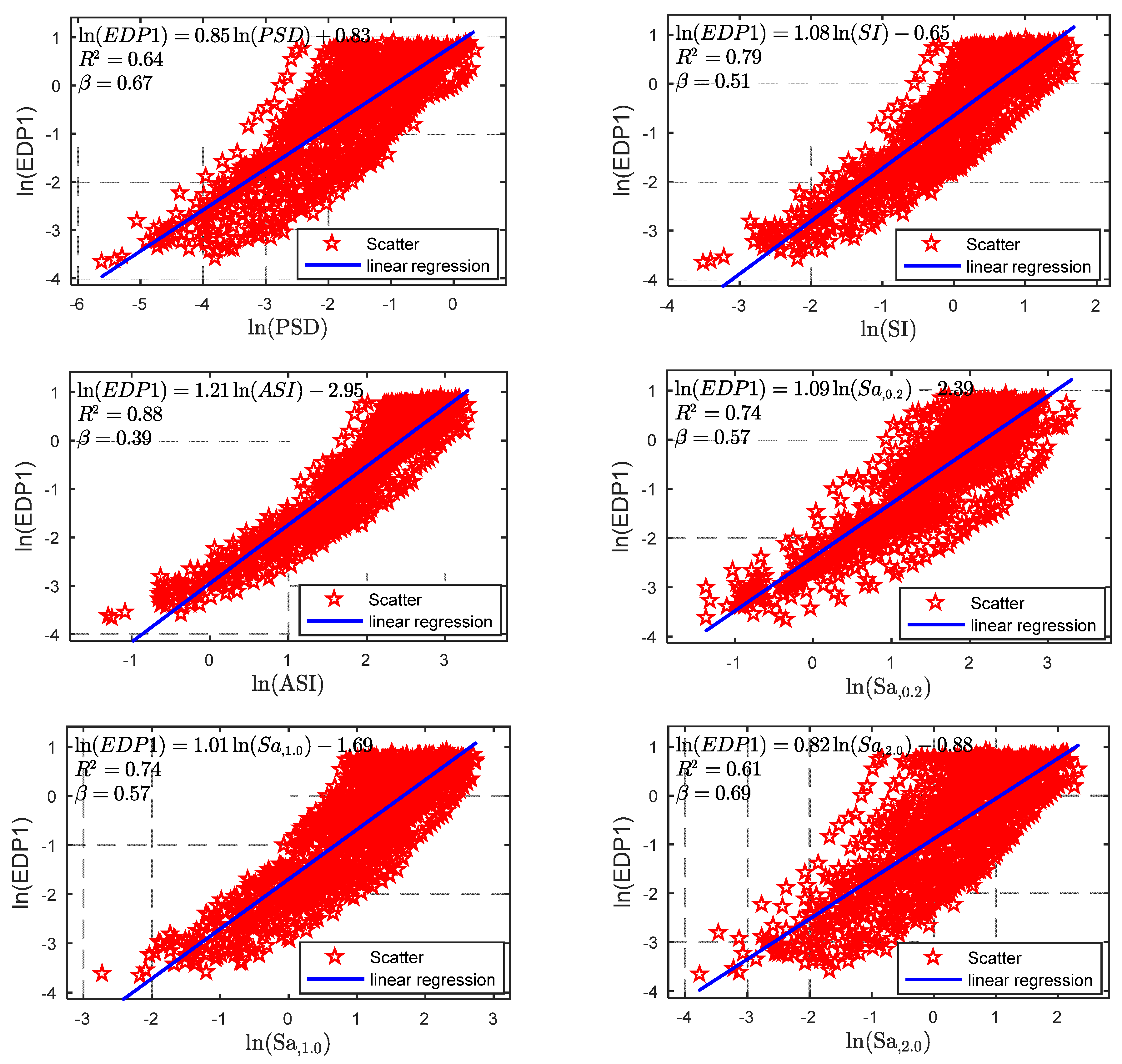
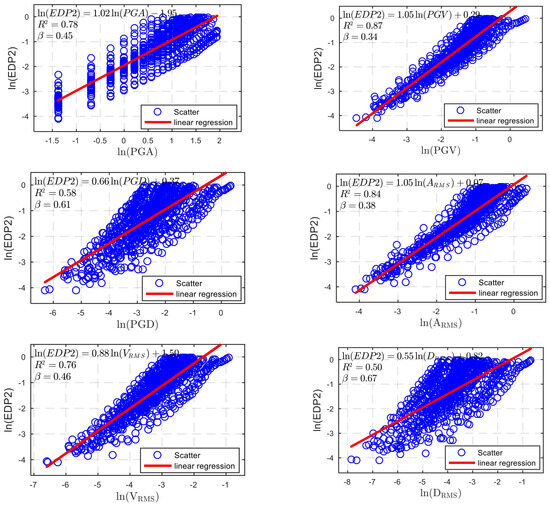
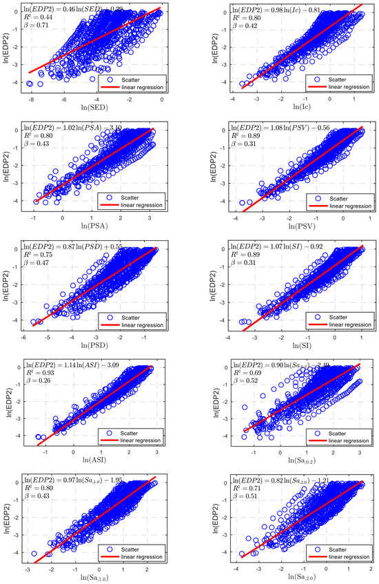
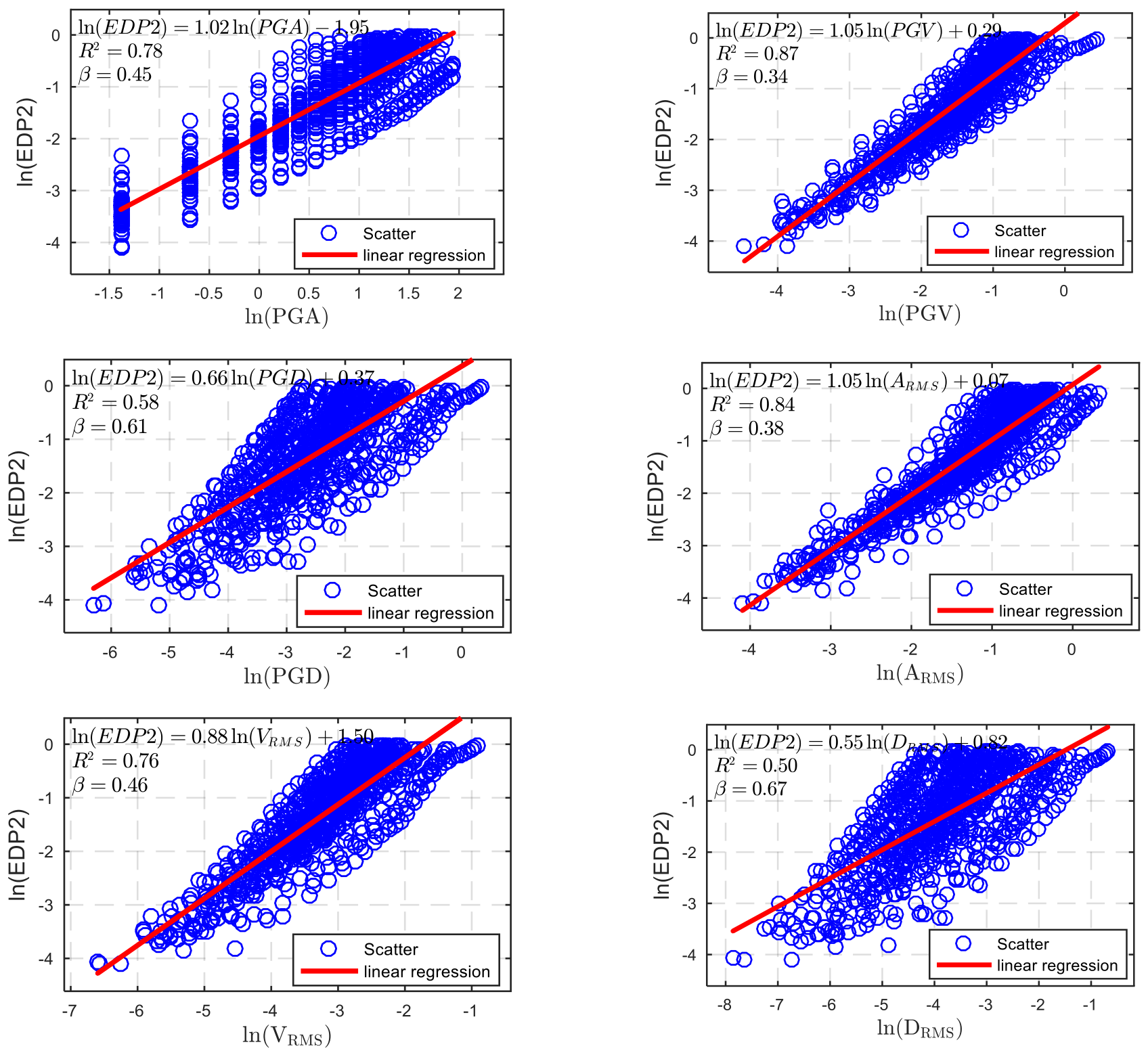
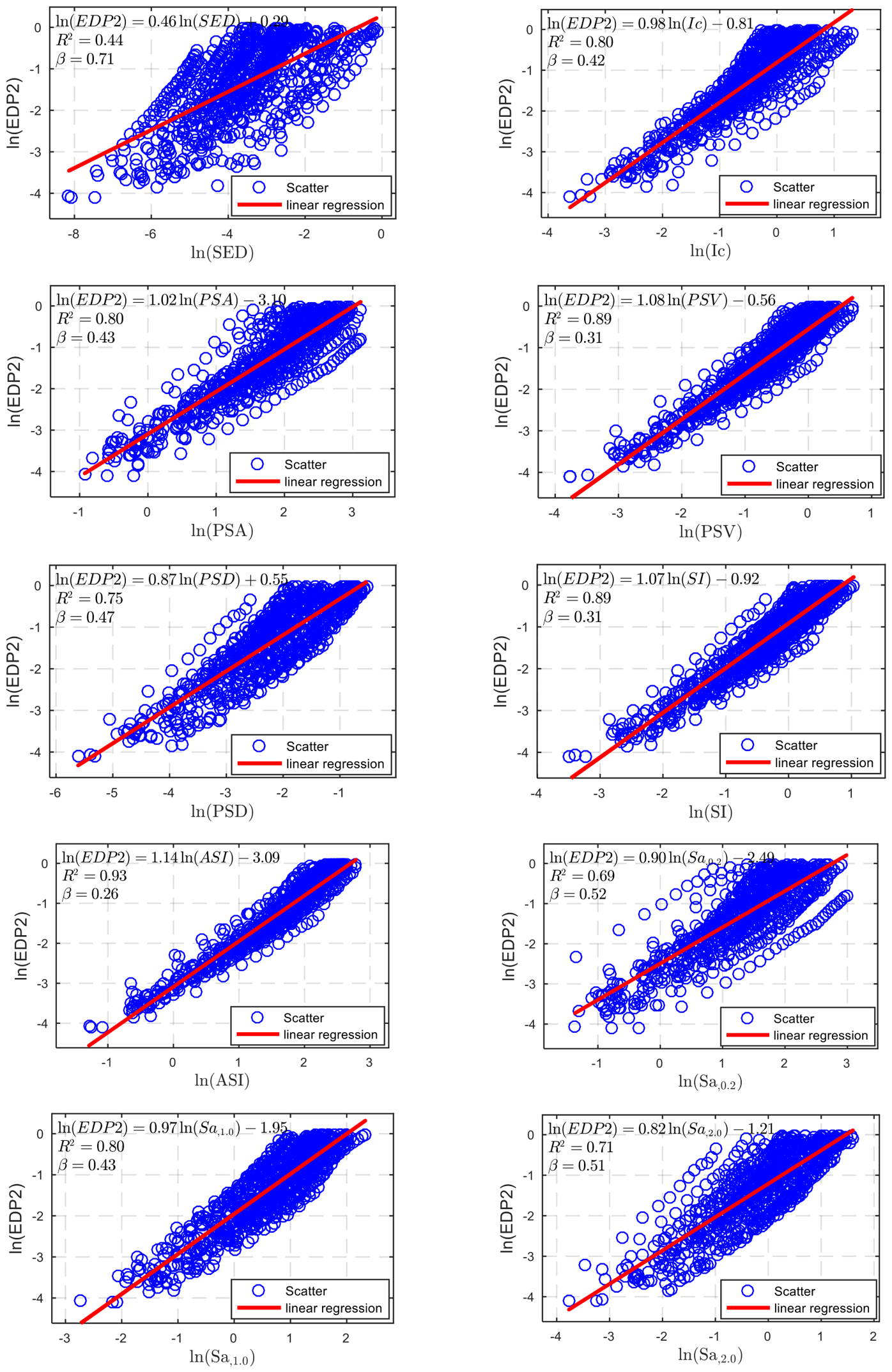
The selection of IMs for the specific EDP is a noteworthy step in the IDA method to build PSDM of the VBI system. This section presents the results of 44 PSDM analyses (22 IMs × 2 EDPs = 44 groups) obtained from combinations of two EDPs and 22 candidate ground motion IMs. Figure 10 and Figure 11 present the PSDM results for a subset of IMs, using derailment coefficient and wheel unloading as EDPs, respectively. The figures display scatter plots of ln(EDP) versus ln(IM) for these selected IMs, along with fitted regression lines, to visually illustrate the EDP–IM relationships. As can be seen, the choice of ground motion IM directly affects the PSDM of the VBI system.
Figure 10.
PSDMs for derailment coefficient with various IMs.
Figure 11.
PSDMs for wheel unloading with various IMs.
6.2. Evaluation of the Efficiency, Practicality, and Proficiency
A linear regression analysis was performed on the IDA data for the derailment coefficient and wheel unloading, and the PSDMs for each IM and EDP were developed. To quantitatively and accurately evaluate the relationships among different IM-EDP combinations, this section presents a comprehensive correlation analysis of different IMs and EDPs in terms of efficiency, practicality, and proficiency. The aim is to identify the optimal ground motion IM for evaluating the safety of vehicles on bridges during earthquakes.
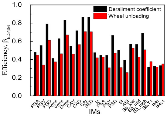
Efficiency: The efficiency reflects the degree of variability of EDPs around the regression model. Figure 12 presents the efficiency results of the relationship between two different EDPs of vehicle response (derailment coefficient and wheel unloading) and 22 candidate IMs.
Figure 12.
Efficiency for the candidate IMs.
Regarding the derailment coefficient, Sa(T1), IMc, IMc1, and ASI are the four most efficient IMs, with values of 0.32, 0.328, 0.333, and 0.39, respectively. SED exhibits the greatest dispersion, with a value of 0.87, making it the least efficient. Next are CAI and DRMS, with corresponding dispersion values of 0.867 and 0.83, respectively, which are slightly lower than that of SED. For the wheel unloading, the ranges from 0.26 to 0.71. Among the 22 candidate ground motion IMs, ASI, PSV, and SI exhibit the best efficiency, with values of 0.257, 0.311, and 0.313, respectively. The larger dispersions are observed for CAI, SED, and DRMS, which show the worst efficiency, with corresponding values of 0.71, 0.706, and 0.67, respectively.
Among the time-history-related and spectrum-related IMs, for the efficiency of the derailment coefficient, acceleration-based IMs performed best, while displacement-based IMs performed worst. In terms of wheel unloading, the velocity-based IM seems to perform better, and displacement-based IMs performed worst. For the two EDPs, i.e., the derailment coefficient and the wheel unloading, it is observed that the efficiency of the wheel unloading is generally higher than that of the derailment coefficient for most of the candidate IMs.
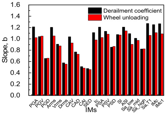
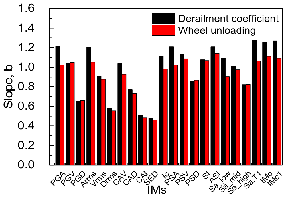
Practicality: Practicality refers to the degree of dependence of the EDPs on the ground motion IMs, which is described by the regression parameter b in Equation (3). A larger value of b indicates a stronger sensitivity between the IM and the vehicle response EDP. This means that the IM can more sensitively reflect the influence of ground motion input on the vehicle response, making it more suitable as an indicator for predicting EDPs.
Figure 13 displays the variation in parameter b for the 22 IMs and different EDPs. As can be seen from Figure 13, for the derailment coefficient, Sa(T1), IMc1, IMc, and PGA are the four IMs with a good practicality. Their corresponding regression parameter b values are 1.273, 1.27, 1.25, and 1.21, respectively. The IMs with the poorest practicality are SED, CAI, and DRMS, with b values of 0.478, 0.511, and 0.578, respectively. For the wheel unloading: Among the 22 candidate IMs, ASI, IMc, and IMc1 show a good practicality, with b values of 1.14, 1.11, and 1.09, respectively. The least practical IMs are SED, CAI, and DRMS, with corresponding b values of 0.46, 0.48, and 0.55, respectively.
Figure 13.
Practicality for the candidate IMs.
Compared to the time-history-related IMs, the spectrum-related IMs are more practical. For the two EDPs, i.e., the derailment coefficient and the wheel unloading, it is observed that for most candidate IMs, the practicality of the derailment coefficient is higher than that of wheel unloading.
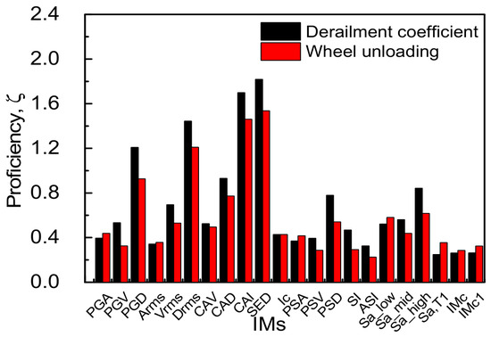
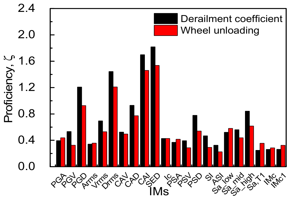
Proficiency: Proficiency (denoted as , see Equation (6)) is a comprehensive evaluation criterion that considers both efficiency and practicality. A smaller value indicates higher proficiency for the corresponding IM. Figure 14 shows the proficiency for the 22 IMs corresponding to the vehicle derailment coefficient and wheel unloading, respectively.
Figure 14.
Proficiency for the candidate IMs.
For the derailment coefficient, Sa(T1) exhibits the highest proficiency, with the smallest value of 0.25; followed by IMc, IMc1, and ASI with values of 0.262, 0.263, and 0.33, respectively. SED, CAI, and DRMS are the three IMs with the lowest proficiency, with corresponding values of 1.82, 1.70, and 1.44, respectively. For the wheel unloading, among the 22 candidate IMs, ASI, IMc, and PSV show a good proficiency, with values of 0.225, 0.286, and 0.287, respectively. The ground motion IMs with the worst proficiency were SED, CAI, and DRMS, with corresponding values of 1.54, 1.46, and 1.21, respectively. As can be seen from Figure 14, the proficiency of spectrum-related IMs is better than that of time-history-related IMs. The Sa(T1) performs the best among the 22 candidate IMs for the derailment coefficient, and ASI performs the best for the wheel unloading.
7. Conclusions
This study aims to identify the optimal IMs for the safety evaluation of vehicles running on bridges during earthquakes. The effects of far-field and near-fault ground motions are considered. Two EDPs (derailment coefficient and wheel unloading) and 22 candidate IMs were introduced to build the PSDM for the VBI system. Different IM-EDP combinations are compared and analyzed from three perspectives: efficiency, practicality, and proficiency. The conclusions are as follows:
- (1)
- For the nonlinear VBI dynamic system, with regard to the EDPs (derailment coefficient and wheel unloading), the relationship between the engineering demand parameters and the ground motion PGA exhibits a power-law curve.
- (2)
- Once the ground motion PGA reaches a critical intensity, hysteretic behavior emerges in the IDA curve. Notably, the hysteresis of the wheel unloading IDA curve is less significant than that of the derailment coefficient.
- (3)
- For the efficiency of the derailment coefficient, acceleration-based IMs performed best, while displacement-based IMs performed worst; In terms of wheel unloading, the velocity-based IM seems to perform better, and displacement-based IMs performed worst.
- (4)
- The proficiency of spectrum-related IMs is better than that of time-history-related IMs. For the vehicle–bridge dynamic system examined in this study, the Sa(T1) performs the best among the 22 candidate IMs for the derailment coefficient, and ASI performs the best for the wheel unloading.
While this framework has been successfully applied to the risk assessment of vehicle running safety on bridges during earthquakes, some limitations should be acknowledged, as a base for future development. (1) This work constitutes a preliminary study on the application of the PSDM frame to vehicle–bridge interaction systems. The applicability of the results is subject to the adopted bridge structures, vehicle type, and operating conditions. The sensitivity of intensity measure ranking to bridge geometry, vehicle type, vehicle speeds, running safety indicators, and track characteristics will be further investigated in future work. (2) The vehicle–bridge interaction model in this study is treated deterministically, and uncertainties in material properties, damping, stiffness degradation, wheel–rail contact, and suspension characteristics are not propagated through the probabilistic seismic demand model.
Author Contributions
Conceptualization, W.L.; methodology, W.L.; software, W.L. and W.Z.; validation, Z.W. and W.Z.; formal analysis, W.L. and W.Z.; investigation, W.Z. and Z.W.; resources, W.L.; data curation, Z.W. and W.Z.; writing—original draft preparation, W.L.; writing—review and editing, W.L., W.Z. and Z.W.; visualization, W.Z. and Z.W.; supervision, W.L.; project administration, W.L.; funding acquisition, W.L. All authors have read and agreed to the published version of the manuscript.
Funding
This research was funded by the Natural Science Foundation of Henan Province (Grant Nos. 242300421458, 252300423427) and the Key Scientific Research Project Plan of Colleges and Universities in Henan Province (Grant No. 24A560010).
Institutional Review Board Statement
Not applicable.
Informed Consent Statement
Not applicable.
Data Availability Statement
The data presented in this study are available on request from the corresponding author.
Conflicts of Interest
The authors declare no conflicts of interest.
References
- Zhang, N.; Tian, Y.; Xia, H. A train-bridge dynamic interaction analysis method and its experimental validation. Engineering 2016, 2, 528–536. [Google Scholar] [CrossRef] [Scilit]
- Montenegro, P.; Carvalho, H.; Ribeiro, D.; Calçada, R.; Tokunaga, M.; Tanabe, M.; Zhai, W. Assessment of train running safety on bridges: A literature review. Eng. Struct. 2021, 241, 112425. [Google Scholar] [CrossRef] [Scilit]
- Gong, W.; Zhu, Z.; Liu, Y.; Liu, R.; Tang, Y.; Jiang, L. Running safety assessment of a train traversing a three-tower cable-stayed bridge under spatially varying ground motion. Railw. Eng. Sci. 2020, 28, 184–198. [Google Scholar] [CrossRef] [Scilit]
- Yang, C.S.W.; Werner, S.D.; DesRoches, R. Seismic fragility analysis of skewed bridges in the central southeastern United States. Eng. Struct. 2015, 83, 116–128. [Google Scholar] [CrossRef] [Scilit]
- Zhou, W.; Xiong, L.; Jiang, L. Multi-parameter seismic fragility analysis of high-speed railway track-bridges: Embracing structural and earthquake uncertainties. Int. J. Struct. Stab. Dyn. 2026, 26, 2630001. [Google Scholar] [CrossRef] [Scilit]
- Meng, D.; Yang, M.; Sun, T.; He, X.; Chouw, N. Seismic-induced poundings in highway and high-speed railway bridges: A state-of-the-art review. Struct. Infrastruct. Eng. 2025, 21, 628–642. [Google Scholar]
- Padgett, J.E.; Nielson, B.G.; DesRoches, R. Selection of optimal intensity measures in probabilistic seismic demand models of highway bridge portfolios. Earthq. Eng. Struct. Dyn. 2008, 37, 711–725. [Google Scholar]
- Zeng, Q.; Dimitrakopoulos, E.G. Seismic response analysis of an interacting curved bridge-train system under frequent earthquakes. Earthq. Eng. Struct. Dyn. 2016, 45, 1129–1148. [Google Scholar] [CrossRef] [Scilit]
- Japan Transport Safety Board. Railway Accident Investigation Report-Train Derailment Accident Between Kumamoto Station and Kumamoto General Train Depot of the Kyushu Shinkansen of the Kyushu Railway Company; RA2017-8-II; Japan Transport Safety Board: Tokyo, Japan, 2017.
- Zhao, H.; Wei, B.; Jiang, L.; Xiang, P.; Zhang, X.; Ma, H.; Xu, S.; Wang, L.; Wu, H.; Xie, X. A velocity-related running safety assessment index in seismic design for railway bridge. Mech. Syst. Signal Process. 2023, 198, 110305. [Google Scholar] [CrossRef] [Scilit]
- Di Mucci, V.M.; Cardellicchio, A.; Ruggieri, S.; Nettis, A.; Renò, V.; Uva, G. Computer vision-based seismic assessment of RC simply supported bridges characterized by corroded circular piers. Bull. Earthq. Eng. 2025, 23, 6771–6800. [Google Scholar] [CrossRef] [Scilit]
- Nguyen, H.D.; Shin, M.; LaFave, J.M. Optimal intensity measures for probabilistic seismic demand models of steel moment frames. J. Build. Eng. 2023, 65, 105629. [Google Scholar] [CrossRef] [Scilit]
- Chen, L.; Zuo, R.; Hu, Z.L.; Xia, W.; Hao, Z.; Hu, Y.; Zhang, Y. Effects of important characteristics of earthquake ground motions on probabilistic seismic demand assessment of long-span cable-stayed bridges. Structures 2024, 60, 105910. [Google Scholar] [CrossRef] [Scilit]
- Zhong, J.; Jeon, J.S.; Shao, Y.H.; Chen, L. Optimal intensity measures in probabilistic seismic demand models of cable-stayed bridges subjected to pulse-like ground motions. J. Bridge Eng. 2019, 24, 04018118. [Google Scholar] [CrossRef] [Scilit]
- Wang, X.; Shafieezadeh, A.; Ye, A. Optimal intensity measures for probabilistic seismic demand modeling of extended pile-shaft-supported bridges in liquefied and laterally spreading ground. Bull. Earthq. Eng. 2018, 16, 229–257. [Google Scholar]
- Wei, B.; Hu, Z.; He, X.; Jiang, L. Evaluation of optimal ground motion intensity measures and seismic fragility analysis of a multi-pylon cable-stayed bridge with super-high piers in Mountainous Areas. Soil Dyn. Earthq. Eng. 2020, 129, 105945. [Google Scholar] [CrossRef] [Scilit]
- Matsuzaki, H. Optimal Intensity Measure Selection for the Life-Cycle Seismic Fragility Assessment of Isolated Bridges. In Life-Cycle Performance of Structures and Infrastructure Systems in Diverse Environments; CRC Press: Boca Raton, FL, USA, 2025; pp. 154–159. [Google Scholar]
- Wang, Y.; Guo, W.; Zeng, C.; Huang, R.; Yang, S.; Nie, Y.; Jiang, L.; Yu, Z. Shaking table study on high-speed train seismic derailment mechanism and verification of spectrum intensity derailment index. Earthq. Eng. Struct. Dyn. 2024, 53, 3287–3317. [Google Scholar] [CrossRef] [Scilit]
- Luo, X. Study on methodology for running safety assessment of trains in seismic design of railway structures. Soil Dyn. Earthq. Eng. 2005, 25, 79–91. [Google Scholar] [CrossRef] [Scilit]
- Railway Technical Research Institute. Design Standards for Railway Structures and Commentary (Displacement Limits); Maruzen Co., Ltd.: Tokyo, Japan, 2006. [Google Scholar]
- Jin, Z.; Liu, W. Fragility analysis for vehicle derailment on railway bridges under earthquakes. Railw. Eng. Sci. 2022, 30, 494–511. [Google Scholar] [CrossRef] [Scilit]
- Liu, X.; Jiang, L.; Xiang, P.; Feng, Y.; Lai, Z.; Sun, X. Evaluation of optimal ground motion intensity measures of high-speed railway train running safety on bridges during earthquakes. Struct. Eng. Mech. An. Int. J. 2022, 81, 219–230. [Google Scholar]
- Akturk, F.; Yesilyurt, A.; Cakir, F. Optimal intensity measures for probabilistic seismic demand modeling of single-domed historical masonry buildings. Eng. Fail. Anal. 2025, 171, 109378. [Google Scholar] [CrossRef] [Scilit]
- Cornell, C.A.; Jalayer, F.; Hamburger, R.O.; Foutch, D.A. Probabilistic basis for 2000 SAC federal emergency management agency steel moment frame guidelines. J. Struct. Eng. 2002, 128, 526–533. [Google Scholar] [CrossRef] [Scilit]
- Zhang, C.; Zhao, M.; Zhong, Z.; Du, X. Optimum intensity measures for probabilistic seismic demand model of subway stations with different burial depths. Soil Dyn. Earthq. Eng. 2022, 154, 107138. [Google Scholar] [CrossRef] [Scilit]
- Giovenale, P.; Cornell, A.C.; Esteva, L. Comparing the adequacy of alternative ground motion intensity measures for the estimation of structural responses. Earthq. Eng. Struct. Dyn. 2004, 33, 951–979. [Google Scholar] [CrossRef] [Scilit]
- Luco, N.; Cornell, C.A. Structure-Specific Scalar Intensity Measures for Near-Source and Ordinary Earthquake Ground Motions. Earthq. Spectra 2007, 23, 357–392. [Google Scholar] [CrossRef] [Scilit]
- Mackie, K.; Stojadinovic, B. Probabilistic Seismic Demand Model for California Highway Bridges. J. Bridge Eng. 2001, 6, 468–481. [Google Scholar] [CrossRef] [Scilit]
- Si, P.; Tang, L.; Tian, S.; Liu, Y.; Ling, X. Probabilistic demand models and fragility analysis of railway embankments subjected to multi-pulse ground motions. Transp. Geotech. 2025, 52, 101522. [Google Scholar] [CrossRef] [Scilit]
- Shen, Y.; El Naggar, M.H.; Zhang, D.; Huang, Z.; Du, X. Optimal intensity measure for seismic performance assessment of shield tunnels in liquefiable and non-liquefiable soils. Undergr. Space 2025, 21, 149–163. [Google Scholar] [CrossRef] [Scilit]
- Nishimura, K.; Terumichi, Y.; Morimura, T.; Sogabe, K. Development of vehicle dynamics simulation for safety analyses of rail vehicles on excited tracks. J. Comput. Nonlinear Dyn. 2009, 4, 011001. [Google Scholar] [CrossRef] [Scilit]
- Zhai, W. Vehicle-Track Coupled Dynamics: Theory and Applications; Springer Nature: Singapore, 2020. [Google Scholar]
- Zhai, W.; Xia, H.; Cai, C.; Gao, M.; Li, X.; Guo, X.; Zhang, N.; Wang, K. High-speed train–track–bridge dynamic interactions–Part I: Theoretical model and numerical simulation. Int. J. Rail Transp. 2013, 1, 3–24. [Google Scholar] [CrossRef] [Scilit]
- Shen, Z.Y.; Hedrick, J.K.; Elkins, J.A. A comparison of alternative creep force models for rail vehicle dynamic analysis. Veh. Syst. Dyn. 1983, 12, 79–83. [Google Scholar] [CrossRef] [Scilit]
- Jin, Z.; Liu, W.; Pei, S. Probabilistic evaluation of railway vehicle’s safety on bridges under random earthquake and track irregularity excitations. Eng. Struct. 2022, 266, 114527. [Google Scholar] [CrossRef] [Scilit]
- Zhai, W.; Chen, G. Method and criteria for evaluation of wheel derailment based on wheel vertical rise. J. China Railw. Soc. 2001, 23, 17–26. (In Chinese) [Google Scholar]
- UIC 530-2; Wagons—Running Safety. International Union of Railways (UIC): Paris, France, 2006.
- Federal Emergency Management Agency. Quantification of Building Seismic Performance Factors: FEMA P695; Federal Emergency Management Agency: Washington, DC, USA, 2009.
- Cordova, P.P.; Deierlein, G.G.; Mehanny, S.S.F.; Cornell, C.A. Development of a two-parameter seismic intensity measure and probabilistic assessment procedure. In Proceedings of the Second US-Japan Workshop on Performance-Based Earthquake Engineering Methodology for Reinforced Concrete Building Structures; Pacific Earthquake Engineering Research Center, University of California: Berkeley, CA, USA, 2000; Volume 20. [Google Scholar]

Disclaimer/Publisher’s Note: The statements, opinions and data contained in all publications are solely those of the individual author(s) and contributor(s) and not of MDPI and/or the editor(s). MDPI and/or the editor(s) disclaim responsibility for any injury to people or property resulting from any ideas, methods, instructions or products referred to in the content. |
© 2026 by the authors. Licensee MDPI, Basel, Switzerland. This article is an open access article distributed under the terms and conditions of the Creative Commons Attribution (CC BY) license.