


Featured Application
The proposed Bayesian multi-model reliability analysis framework can be applied to safety assessment and reliability-based design of engineering structures involving scarce data and complex dependent random variables, such as aerospace, mechanical, and civil infrastructure systems.
Abstract
This paper investigates the epistemic uncertainty associated with dependence modeling and its impact on structural reliability analysis when data for vine structure selection is limited. Conventionally, the vine copula model characterizing dependent input variables in reliability analysis is typically assumed to be either a single model or the optimal fit model obtained from the data. However, subjective assumptions and data scarcity may introduce bias into correlation measurements, causing significant deviations between the vine structure and the actual dependence structure, as well as substantial errors in reliability analysis. In this paper, we address model uncertainties in vine structures arising from sparse data by introducing Bayesian multi-model inference. This approach identifies the corresponding Bayesian posterior probabilities for an ensemble of candidate vine structures based on their overall dependence modeling performance. Utilizing the Bayes factor to screen effective candidate vine structures, a reweighted model set is formed to quantify model uncertainty in dependence modeling. The integrated first-order reliability method for regular vine copulas provides both precision and high efficiency in reliability analysis. Finally, numerical and engineering examples demonstrate that the proposed method yields more accurate and robust reliability analysis results across various sample sizes in contrast to a single optimal vine copula model.
1. Introduction
In the field of structural reliability analysis, uncertainty is a critical factor affecting structural performance and safety. Based on their sources and nature, uncertainties are typically classified into two types: aleatory and epistemic uncertainty. Aleatory uncertainty stems from the intrinsic randomness in a physical system, while epistemic uncertainty arises due to insufficient knowledge or data about the system [1,2]. Specifically, aleatory uncertainty represents variabilities in material properties, loading conditions, or structural geometry, typically characterized by probabilistic models. Based on probabilistic models, numerous reliability analysis methods were proposed [3], such as Monte Carlo Simulation (MCS) [4,5], the first-order reliability method (FORM) [6,7,8], and the second-order reliability method (SORM) [9,10]. In current reliability analysis, random variable inputs are often assumed independent for simplicity. However, in practice, correlations commonly exist among input variables, and ignoring these correlations can significantly affect the outcomes of structural reliability analysis [11]. The primary techniques currently used to address correlations among input variables include the Nataf transformation [12], the Rosenblatt transformation [13], and the principal component analysis [14,15]. However, the above approaches typically rely on specific assumptions and linear or even symmetric correlation structures, which limit their applicability to complex, nonlinear, or non-Gaussian dependencies. Therefore, to overcome the limitations of existing approaches, it is crucial to build an efficient reliability analysis method that enhances flexibility and applicability in handling input variable dependencies.
In recent years, copula functions have emerged as an effective and flexible tool in uncertainty analysis to handle correlations between variables. Initially proposed by Sklar [16], copula functions serve as linking functions connecting marginal distributions to joint distributions. Building upon this foundation, scholars introduced the pair copula functions, subsequently developing the regular vine copula (RVC) model [17]. The vine copula model decomposes the multivariate joint distribution into the product of pair-copula functions and marginal distributions. Compared to traditional methods, the vine copula model accommodates more generalized distributions of random variables, does not require complete probability information, and can handle nonlinear or tail dependencies between variables. Currently, copula functions and related dependence modeling methods have found extensive applications in finance [18], hydraulic engineering [19], maintenance optimization [20], reliability analysis [21,22,23,24] and other fields [25]. Heresi [26] incorporated the evaluation of the effect of damage correlation between structures into seismic risk assessment through copula functions. Wen [27] employed copula functions to investigate the distribution of seismic responses in substation equipment, finding that the selection of copula functions significantly influences the characterization of nonlinear correlations, and the incorporation of copula functions enables more stable seismic vulnerability assessments. Yang [28] introduced the vine copula to incorporate inherent correlation among material properties within slope reliability analysis and revealed that neglect of such correlations increases the failure probability. Fan [29] considered segmented dependencies based on the vine copula function to evaluate the multiple failure modes of a gear transmission system. Meanwhile, the rapid growth of the vine structure space remains a major challenge in high-dimensional vine copula modeling. Regularized and sparse vine-selection methods have therefore been developed to reduce the number of active pair copulas and alleviate the need for exhaustive structure enumeration [30,31].
Despite significant advancements in vine copula methods for structural reliability analysis, the above studies often rely solely on a single predetermined pair-copula or vine copula model. However, the specific type of copula function and the dependence structure among variables are normally unknown in most cases, and thus the impact of model uncertainty, such as the choice of copula function, on reliability analysis is also a challenging problem. Model uncertainty falls under epistemic uncertainty, primarily stemming from insufficient information, such as data scarcity or lack of knowledge. In the development of a vine copula model, epistemic uncertainty manifests specifically in three aspects: the construction of the vine structure, the selection of pair-copula functions, and the estimation of copula dependence parameters. These model uncertainties in vine copula modeling impact the characterization of dependencies among random variables, thereby significantly affecting structural reliability analysis. Wang [32] proposed a dependence modeling method incorporating different bivariate copulas and emphasized the importance of accurate characterization of dependence structures. Liu [33] examined the impact of six distinct vine structures on aerospace structural reliability analysis, revealing that the choice of vine copula model may introduce significant errors in failure probability and the reliability index. Although these studies demonstrated that different copula models significantly influence reliability analysis outcomes, establishing feasible multivariate dependencies with incomplete information, particularly with scarce data, still requires further research.
In uncertainty analysis, Bayesian modeling and related uncertainty modeling methods have found broad applications in reliability engineering, global sensitivity analysis [34], information fusion [35], and other fields. For example, when dealing with uncertainties in material properties, Bayesian estimation can be used to capture Weibull distribution parameters for various materials [36,37]. Furthermore, the Bayesian framework can be integrated with reliability analysis methods to significantly improve the computational efficiency and accuracy of structural safety assessments [38]. Given the widespread application of Bayesian frameworks, there has been growing interest in combining Bayesian inference with dependence modeling. Recently, Bayesian multi-model inference [39,40,41] has been employed as a novel and effective tool to address model uncertainties in copula modeling. Zhang [42,43] proposed a framework that employs a Bayesian weighted model ensemble encompassing all plausible candidate models to retain and propagate the uncertainties related to model selection and parameter estimation. In the subsequent uncertainty analysis, this approach investigated the impacts of dataset size on dependence modeling and response statistics. Kumar [44] introduced Bayesian multi-model inference (BMMI) into slope analysis to account for model uncertainty in copula models and variable marginal distributions facing small sample sizes of inputs. Sheng [45] employed mixed copula functions to capture the joint probability distribution of wind and temperature effects on bridge performance. By integrating the EM algorithm with the Bayesian selection method, the weights of the mixed copula functions were effectively identified, enabling precise evaluation of joint action reduction. While existing research has explored model uncertainties related to copula functions and parameter estimation, there is a lack of studies on the uncertainty associated with the structure of vine copula in the current literature. Establishing the vine structure is a crucial first step in vine copula modeling. Therefore, investigating the impact of uncertainty in vine structure on dependence modeling and reliability analysis is extremely important.
This paper proposes a structural reliability analysis method based on the regular vine copula model to capture the nonlinear multivariate correlations among input variables. The epistemic uncertainty associated with vine copula structure selection is addressed through an ensemble of candidate models under the framework of Bayesian multi-model inference, enabling structural reliability analysis with limited data. The contributions of this paper are as follows: (1) A structural reliability analysis framework is developed to capture complex multivariate dependencies among input variables using regular vine copula models. (2) Both aleatory uncertainty of input variables and epistemic uncertainty of vine copula structures are effectively incorporated into the reliability assessment. (3) Bayesian multi-model inference utilizes a candidate model ensemble approach to address model uncertainty induced by limited data in vine copula selection.
The structure of this paper is organized as follows: Section 2.1 outlines the fundamentals of copula functions; Section 2.2 proposes a structural reliability analysis method that integrates the regular vine copula model with FORM; Section 2.3 presents a Bayesian multi-model inference approach for handling the epistemic uncertainty associated with vine structures; Section 3 illustrates the BMMI method through numerical and engineering examples; and Section 4 offers a summary of the paper’s contributions.
2. Methodology
2.1. Fundamentals of Copula Functions
Copula functions characterize dependencies among random variables by connecting multivariate joint distribution to its respective univariate marginal distributions. According to the Sklar theorem [46], for an n-dimensional random vector with marginal distributions , the joint cumulative distribution function (CDF) F can be represented by Equation (1):
where C is the copula function associated with F. The joint probability density function (PDF) f can be formulated using Equations (2) and (3):
where is the PDF of and c is the density function of C.
The conventional measurements, such as Pearson’s linear correlation coefficient and Kendall’s rank correlation coefficient (Kendall’s tau), tend to reduce dependence between variables to a single scalar. In contrast, the copula function captures the entire joint correlation structure independently of the marginal distributions, enabling the modeling of asymmetric, nonlinear, and tail dependence patterns. More importantly, the copula function enables the generation of synthetic data that accurately reflect the dependencies present in the original dataset. In addition, the copula function has the following relationship with Kendall’s tau [33]:
where denotes the Kendall’s tau between variables and , denotes the corresponding copula dependence parameter. The parameter can be directly obtained from Equation (4) or estimated by the maximum likelihood method.
2.1.1. Bivariate Copula Functions
Initially, the copula functions were proposed to capture the correlation between two variables. Among the most widely applied bivariate copula functions are the elliptic and Archimedean families. The elliptic copula functions primarily include the Gaussian copula and the t-copula, both of which are equivalent to their corresponding multivariate distributions. Within the Archimedean class, the Frank, Clayton, and Gumbel copulas are mostly favored. Notably, the Clayton and Gumbel copula functions can capture asymmetric tail dependence and describe heavy-tailed characteristics [47]. In contrast, the Frank copula function and the elliptic copula functions mentioned above do not exhibit asymmetric tail dependence.
Copula functions exhibiting unequal tail dependencies are often termed asymmetric copulas. Asymmetry introduces directionality, and when describing different tail characteristics using asymmetric copula functions, it becomes necessary to introduce rotated copula functions. The asymmetric copula functions can be rotated by 90°, 180°, and 270° to capture various correlations, including positive and negative correlations as well as upper and lower tail dependencies. Particularly, the copula functions after 180° rotation are called survival copula functions. For variables and with joint distribution , the rotated copula functions can be described as Equation (5):
In this paper, Gaussian, t, Frank, rotated Clayton, and rotated Gumbel copulas are employed as candidate functions for pair-copula selection. The corresponding copula functions are also listed in Table 1.
Table 1.
Common bivariate copula functions [46].
2.1.2. Regular Vine Copula Model
As the dimensionality of random variables grows, the multidimensional correlations between variables become more complex, requiring more flexible and advanced tools. The vine copula function decomposes the multivariate joint PDF into bivariate copula functions along with their corresponding conditional copula functions. For an n-dimensional random vector , the multidimensional PDF can be expressed by Equation (6) [46]:
where denotes the conditional PDF. For three variables, one possible case can be [21]:
where denotes the density of the conditional pair-copula , characterizing the dependence between and conditional on ; and denote the corresponding CDFs.
The conditional CDFs corresponding to Equations (7) and (8) are commonly referred to as h-functions [47], representing the bivariate conditional distribution as Equation (9):
where and . Therefore, the conditional copula density can also be written as or .
In this study, the simplifying assumption is adopted for all conditional pair copulas [48]. Specifically, for the conditional copula density , the copula family and its parameter are assumed to be invariant with respect to the values of the conditioning variable . Nevertheless, the conditioning variables still affect the copula density through the conditional probability arguments.
As shown in Equations (7) and (8), the sequence of conditional functions established here is merely illustrative; other sequences are also acceptable. In fact, there are numerous ways to decompose a multivariate PDF. To illustrate decomposition methods and the relationships between the variables being characterized more directly, Bedford and colleagues proposed the vine model [49,50]. This graphical model can explicitly depict different decomposition processes. The vine model can be freely designed but must satisfy the following conditions: Use n-1 edges to connect all n nodes without forming any cycles. For n variables, the vine model consists of n-1 trees. In each layer of the tree, nodes are symbolized by circles, while the connecting lines between two nodes are referred to as edges. Edges from the previous layer naturally serve as nodes in the current layer, forming a layered structure that gradually shortens from top to bottom.
The most common vine copula models are two special cases of the regular vine (R-Vine) copula: the Canonical vine (C-Vine) model, which employs a central node strategy, and the Drawable vine (D-Vine) model, which connects variables sequentially in pairs. The specific tree structures of all layers in these two vine copula models are illustrated in Figure 1. Researchers widely adopt both models due to their intuitive and straightforward structures. Unfortunately, this predefined graph structure may link weakly correlated variables while overlooking truly significant and closely related ones. Therefore, to investigate how the graphical structure of vine models impacts multivariate correlation modeling, this paper addresses vine graphical models starting from the more general regular vine model, with one possible structure shown in Figure 2.
Figure 1.
Five-variable C-Vine and D-Vine models.
Figure 2.
A five-variable Regular vine (R-Vine) model.
Furthermore, to simplify the representation of vine structures, this paper introduces the vine array [47]. A vine array is typically an upper or lower triangular matrix whose dimension matches the number of variables. A single vine array is sufficient to represent the whole structure of all layers of a vine model. For example, the vine arrays and corresponding to the C-Vine and D-Vine models in Figure 1 can be expressed as Equation (10):
Taking the C-Vine copula as an example, by examining specific tree structures in all layers of the vine copula model through the process depicted in Figure 3, the vine array can be obtained by following these steps:
Figure 3.
Assembly process of the vine array for C-Vine model.
- Determine the diagonal elements of the vine array, such as (1, 2, 3, 4, 5);
- The remaining elements in the first row indicate the nodes connected to the diagonal elements within the first tree (Tree 1). For example, edge 12 places 1 in the first row of the same column as diagonal element 2;
- The remaining elements in the second row represent the nodes connected to the diagonal elements, conditioned on the elements in the same column from the previous row. For example, edge 24|1 places 2 in the second row of the same column as diagonal element 4, and the conditional element is 1 in the first row;
- Repeat the steps above;
- Until the n − 1 row, then the complete vine array is obtained.
However, when constructing the R-Vine copula, the central node may not necessarily be 1. As shown in Figure 2, the central node of this R-Vine structure is 3, and the corresponding vine array should be:
In this case, the sequence of diagonal elements in the vine array has been disrupted. It is more common to sort the diagonals of the vine array, as this facilitates both visual inspection and numerical computation. Transforming the sequence (3, 2, 4, 5, 1) into (1, 2, 3, 4, 5) fully preserves the vine structure information. However, the correlation matrix of variables may become misaligned, necessitating a subsequent reverse transformation to restore the original state. The corresponding vine array is shown below:
2.2. Structural Reliability Analysis Based on Regular Vine Copula Models
2.2.1. The Construction of Joint PDF
Considering the n-dimensional random vector , its limit state function (LSF) of a certain structure can be formulated by Equation (13):
Subsequently, the failure probability of the corresponding structure can be obtained by Equation (14):
where represents the failure domain .
In practical structural reliability analysis, random variables typically exhibit multidimensional correlations. Therefore, the vine copula model can be utilized to build the multivariate joint PDF. Combined with MCS or FORMs, this approach yields a reliability index or failure probability for the problem.
According to Section 2.1, the joint PDF that captures multivariate correlations can be decomposed into bivariate copula functions and marginal PDFs using a vine copula model. While much effort has been devoted to selecting marginal distributions for random variables, the crucial step of constructing the joint PDF lies in choosing suitable two-dimensional copula functions and determining the corresponding parameters for these copula functions.
When constructing joint PDFs from data, the copula dependence parameter is typically estimated from Kendall’s correlation coefficient as Equation (4) or maximum likelihood estimation (MLE) by Equation (15):
where is the estimated value of correlation parameter , m is the number of samples, and c is the density function of C.
After obtaining the correlation parameters for all candidate copula functions, the optimal copula function can be selected using the AIC or BIC criteria:
where k is the number of correlation parameters in copula functions. The AIC criterion is relatively concise, while the BIC criterion accounts for the influence of sample size on model selection to prevent overfitting. A lower AIC or BIC value suggests that the copula function better captures the features of the sample data.
In summary, Figure 4 outlines the process for building a joint PDF by the vine copula model. The detailed steps are as follows:
Figure 4.
Construction of joint PDF using the vine copula model.
- Step 1:
- Decompose the joint PDF into bivariate copulas and univariate marginal PDFs, following the tree structures of the vine copula model.
- Step 2:
- Utilize the data samples to estimate the correlation parameters for all plausible copula functions in Tree 1, followed by selecting the optimal copula function using the AIC or BIC criterion.
- Step 3:
- Utilize the h-functions to generate the required data format from data samples, then obtain the optimal copula functions and corresponding correlation parameters within Tree 2.
- Step 4:
- Repeat Step 3 until reaching Tree n − 1.
2.2.2. The RVC-FORM Algorithm
When using the MCS method to solve for failure probability, Equation (14) can be rewritten as:
where is the indicator function for the failure domain. After the construction of joint PDF in Section 2.2.1, sets of samples can be generated for the random vector . Then the MCS value of can be computed by Equation(19):
where represents the number of samples falling in the failure domain.
This paper employs a combination of the FORM and vine copula model to solve reliability analysis problems more efficiently. The Rosenblatt transformation [13] is first performed to map the random vector in the sample space to the independent vector in the standard normal space:
where represents the CDF of the standard normal distribution. The above transformation relies on the simplifying assumption introduced in Section 2.1.2. If this assumption is violated, the conditional copula parameters may vary with the conditioning variables. In this case, the h-functions and Rosenblatt transformation used in the present method would require conditioning-dependent formulations; otherwise, the model weights and reliability estimates may be biased. Although the proposed framework can be extended to non-simplified vines, such an extension requires substantially more data and computational cost, and the present implementation is therefore restricted to simplified R-vine models.
Subsequently, through the following iteration, the independent vector can be obtained [21]:
- Iteration 1:
- Obtain marginal distributions for random variables ;
- Generate an independent vector that follows a uniform distribution from the multidimensional space [0, 1];
- Let , then ;
- Let , from Equation (9), , then ;
- Let , from Equation (9), , then ;
- Let
- , then ;
- Repeat the above steps until ;
- Obtain in the standard normal space.
Subsequently, the reliability analysis can be solved as an optimization problem in the standard normal space, defining the reliability index as Equation (21):
where and is the LSF in the standard normal space. Through the above optimization process, the optimal solution can be found, and the corresponding reliability index can be computed. Then the failure probability can be obtained by Equation (22):
This paper employs the improved HL-RF (iHL-RF) algorithm [51,52] to address the optimization task posed by Equation (21). When searching for the most probable point (MPP), the iHL-RF algorithm continuously approximates the optimal solution through a series of iterations. Based on the Armijo criterion [53], the iHL-RF algorithm can adaptively adjust the step size factor for each iteration step, effectively reducing the number of oscillations and ensuring iterative convergence. Specifically, the algorithm uses a non-differentiable evaluation function as the objective function and searches for the MPP through the following optimization problem [54]:
where . The Armijo criterion typically employs the following iterative updates to optimize the problem in Equation (23):
where denotes the search step size, denotes the search direction, and denotes the gradient vector. To calculate in each iterative step, its relationship with the gradient of the LSF in the sample space can be utilized:
where is the Jacobian matrix, and its specific elements are [21]:
where is the standard normal PDF. When , can be obtained according to Equation (7); when , can be approximated by the following numerical differentiation:
where is the difference step length [33].
Figure 5 summarizes the above process, while the detailed implementation of the RVC-FORM algorithm proceeds as follows:
Figure 5.
Flowchart of the RVC-FORM algorithm.
- Step 1:
- Utilizing Equations (2) and (8), the multivariate joint PDF is decomposed into the product of marginal PDFs and two-dimensional copula functions.
- Step 2:
- Using the AIC or BIC criterion, obtain the optimal copula functions and determine their corresponding correlation parameters in every tree layer, ultimately constructing the joint PDF by the vine copula model.
- Step 3:
- Initialize the iterative starting point as .
- Step 4:
- Use Iteration 1 to map in the sample space to in the standard normal space.
- Step 5:
- Use Equation (25) to compute .
- Step 6:
- For the next iteration step , compute by Equation (24).
- Step 7:
- Use the inverse process of Iteration 1 to obtain in the sample space.
- Step 8:
- If the convergence condition is satisfied, the algorithm ends; otherwise, proceed to Step 5.
- Step 9:
- Obtain the reliability index from the RVC-FORM algorithm and calculate the failure probability by Equation (22).
It is vital to emphasize that in the RVC-FORM algorithm, the sequence of variables must be strictly preserved during the computation of LSF and its gradients. However, as described in Section 2.1.2, after constructing the vine model using R-Vine, the central node in the vine copula tree can be arbitrary, potentially disrupting the variable sequence. Therefore, to obtain correct results, variables must be converted back to their original sequence at Step 5.
2.3. Bayesian Multi-Model Inference of Vine Structure
2.3.1. Model Uncertainty of Vine Structure
In structural reliability analysis, modeling the correlation among input random variables using a vine copula model usually relies on subjective assumptions [55] or best-fit algorithms [56]. However, this approach ignores the impact of vine structure uncertainty on the modeling of multivariate correlations.
As an epistemic uncertainty, the uncertainty of vine structures primarily stems from insufficient data and the lack of relevant knowledge. For example, when calculating Kendall’s tau between variables using sample data, the sample size significantly affects the correlation coefficients. Assuming the correlation between two variables is described by a Gaussian copula with a Kendall’s tau of 0.33, the estimations of Kendall’s tau based on various sample sizes are shown in Figure 6. As the sample size increases from 2 to 500, the estimated Kendall’s tau gradually converges toward the actual value. However, when the sample size is small, particularly below 100, the estimates exhibit significant divergence and render sample-based observations unreliable.
Figure 6.
Influence of sample size on the estimation of Kendall’s tau.
In addition to the subjective assumption of vine structure, common search approaches include greedy algorithms [57,58], Monte Carlo tree search [59], reinforcement learning [60], and other methods. However, these methods typically seek to identify a single best-fitting or “optimal” structure from the available data. Among them, the Maximum Spanning Tree (MST) algorithm is the most widely used and computationally efficient greedy approach, in which pairwise dependence measures—commonly the absolute Kendall’s tau—are used as edge weights to construct the vine structure [61]. Due to the sequential nature of the vine structure, the deeper-layer trees rely heavily on the preceding trees. The MST algorithm identifies a locally optimal vine structure by sequentially maximizing the internal correlation at each tree level. However, when data are scarce, the correlation coefficients computed by samples may deviate markedly from the actual values. This deviation may occur between any pair of variables, leading to different weight rankings in the MST algorithm. Therefore, as illustrated in Figure 7, two sample sets drawn from the same model may yield substantially different Tree 1 structures and, consequently, markedly different “optimal” vine structures, both of which may deviate considerably from the actual vine structure.
Figure 7.
Possible Tree 1 structures of six-dimensional vine copula model.
Furthermore, as shown in Figure 8, the number of plausible vine structures increases exponentially with the number of variables. Even Tree 1 alone has possible configurations for an n-dimensional problem. More generally, the total number of available R-vine structures reaches [62]. To quantify the computational cost associated with this combinatorial growth, we measured the time required to enumerate all plausible vine structures for dimensions n = (5, 6, 7) and extrapolated the results up to n = 15 in proportion to the corresponding theoretical numbers of vine structures. As shown in Table 2, enumerating all seven-dimensional vine structures requires approximately 8.66 s, whereas the estimated enumeration time increases to tens of minutes for the eight-dimensional case and rapidly becomes computationally prohibitive at higher dimensions. Importantly, these estimates account only for structure enumeration and exclude the additional costs of pair-copula family selection, parameter estimation, and reliability analysis.
Figure 8.
Explosion of R-Vine structure search space.
Table 2.
Number of R-vine structures and enumeration time at different dimensions.
Therefore, scalability remains an intrinsic challenge in high-dimensional vine copula modeling. The principal difficulty is that the complete structure space can no longer be enumerated once the dimension becomes moderately large. In reliability analysis, this burden is further increased by dependence-model fitting, probabilistic transformation, and reliability calculation. This study therefore focuses on five- and six-dimensional problems, for which complete enumeration and RVC-FORM calculations remain computationally tractable. Extending the framework to ten or more variables requires dedicated structure-search and sparsification strategies, including:
- (a)
- Advanced structure-search methods. In addition to the approaches discussed above, metaheuristic algorithms can simultaneously explore multiple regions of the structure space, enabling efficient searches in large, high-dimensional combinatorial spaces [63,64]. Lasso-based methods shrink weak conditional relationships to zero and replace structure enumeration with computationally efficient regularized regression, making them suitable for high-dimensional vine construction [30].
- (b)
- Truncated vines. A vine truncated after Tree k sets all pair copulas in higher trees to independence, reducing the leading-order fitting burden from O(d2) to approximately O(kd). For example, a full 15-dimensional vine contains 105 pair copulas, whereas a three-tree truncated vine contains only 39, corresponding to a 62.9% reduction in edgewise fitting operations.
- (c)
- Sparse vines. Thresholded vines provide a more flexible alternative to tree-level truncation by setting only weakly supported pair copulas to independence [31]. Unlike uniform tree-level truncation, this edgewise strategy can retain strongly supported conditional dependencies in higher trees while removing negligible dependencies at any tree level.
These approaches provide technically feasible routes for extending the present framework. However, the truncation level or sparsity threshold must be carefully validated because excessive simplification may omit relevant higher-order conditional or tail dependence.
In addition to the computational burden, limited data pose another substantial inferential challenge. Small samples may contain insufficient information to distinguish among multiple plausible vine structures, making the underlying dependence structure difficult to identify reliably. Consequently, selecting a single “optimal” vine structure may introduce substantial model uncertainty and lead to unstable estimates of the reliability index and failure probability. This motivates the following framework, which retains and averages multiple plausible vine structures.
2.3.2. Bayesian Multi-Model Inference
To address this challenge and establish a more reasonable vine copula model with limited data, this study employs Bayesian multi-model inference [41] to capture dependencies among variables comprehensively. Rather than selecting a single model, BMMI believes that all candidate models have their own probabilities of being the “true” model. Bayesian multi-model inference fundamentally involves employing a set of candidate models , each assigned a corresponding probability to represent the sample data D. This study selects models based on the BIC criterion, utilizing the Bayes factor [65,66], which is the ratio of the integrated likelihood functions for model set . Thus, Equation (17) can be rewritten as:
where denotes the maximum likelihood of model , k denotes the number of parameters and m is the number of samples in dataset D. The model with the lowest BIC is regarded as the best-fitting among all plausible candidates for representing dataset D.
The Bayesian framework enables the assessment of model selection uncertainty and establishes rankings according to the descriptive capabilities of candidate models. According to Bayes’ theorem, the posterior model probability can be derived as [34]:
where is the posterior probability of model , denotes the marginal likelihood of model and is the prior probability of model .
Direct evaluation of the marginal likelihood, or model evidence, generally requires integration over the model parameter space and can be computationally demanding when numerous candidate vine structures are considered. Following Zhang and Shields [67], a Laplace expansion around the maximum-likelihood estimate gives:
where the O(1) term collects the prior- and local-curvature-dependent contributions that remain bounded as m increases, including the log-determinant of the normalized Hessian, the parameter prior density evaluated near the likelihood mode, and the higher-order remainder of the Laplace expansion. These terms are omitted in the BIC approximation, which therefore provides a large-sample approximation to the marginal likelihood rather than an exact evaluation. The applicability and stability of this approximation under limited sample sizes are further examined in the subsequent numerical examples.
In the absence of prior information, all candidate models are given the same priority, meaning each vine structure is assigned a non-informative prior probability . Since , BIC values can be employed to compute the approximate posterior probability of a specific model within the candidate model set [44,68,69], as shown below:
where denotes the difference between the BIC of the ith model and the smallest BIC in the model set. A higher posterior probability indicates that the model better fits the dataset D.
However, the number of plausible vine structures remains substantial: 480 for five-dimensional variables and 23,040 for six-dimensional variables. As the dimension of random variables increases, conducting structural reliability analysis for all candidate structures remains a challenging task. In this paper, to account for the effective contributions of candidate models more efficiently, we adopt the Bayes factor to truncate them. The Bayes factor can be expressed as:
where the Bayes factor denotes the ratio of the posterior probabilities of ith and jth candidate models. If > 3, the data provide stronger evidence for than ; if > 20, is decisively stronger than and the contribution of is negligible.
The vine copula structure constitutes a crucial step in dependence modeling and reveals the connections between the most strongly correlated variables. This paper focuses on the model uncertainty of the vine structure and examines its impact on structural reliability analysis. Following the strategy of sequentially generating vine structures based on the MST algorithm, the first tree provides the primary dependence foundation and constrains the generation of subsequent trees. Therefore, considering model uncertainty at the full-vine level or only at the first tree level may lead to different effects on model selection. Moreover, due to the exponential form of Equation (31) and the multiple levels of the vine structure, the total BIC value of the vine structure may concentrate posterior weights on only a few candidate models, thereby limiting the effectiveness of multi-model inference. Hence, it is necessary to discuss the appropriate level for incorporating vine structure uncertainty and the applicability of Equation (31).
Since the BIC criterion is mainly used to evaluate copula selections in vine copula models, the total BIC can be averaged over the number of edges to measure the overall fitting performance of vine structures, denoted as edge-averaged BIC (EAB). As shown in Figure 9a, with a Bayes factor of 20, EAB retains more candidate models than the total BIC, indicating that EAB-based weights can account for more comprehensive model uncertainty. Moreover, considering the full vine structure yields more candidate models than considering only the first tree, suggesting that the uncertainty in deeper-level trees should not be neglected. Figure 9b further shows that only the combination of EAB-based weights and full-vine model uncertainty prevents posterior weights from concentrating on a few dominant models, thereby enabling more effective multi-model inference.
Figure 9.
Effects of BIC scaling on model selection: (a) mean candidate vine structures; (b) mean largest Bayesian posterior weight.
Therefore, the Bayesian posterior probability of each candidate vine structure can be reformulated from Equation (31) as follows:
where denotes the edge-averaged BIC value of ith vine structure, denotes the difference between the EAB value of ith vine structure and the smallest EAB value in the candidate model set. Similar to the BIC criterion, a lower EAB value indicates the ith vine structure is more likely to fit the dataset D.
In this paper, the Bayes factor of 20 is adopted to determine the top vine structures as the effective candidate models. Through BMMI, the vine copula models based on these vine structures are comprehensively considered, and Bayesian posterior weights are used to integrate the reliability outputs from each model. The complete flowchart of the BMMI reliability analysis method is summarized in Figure 10, and the specific steps are outlined:
Figure 10.
Flowchart of Bayesian multi-model inference reliability analysis method.
- Step 1:
- Draw N samples from MCS or practical engineering problems and calculate the Kendall’s correlation matrix .
- Step 2:
- Generate all plausible vine structures, determine copula families/parameters, calculate their EAB values, and assign corresponding Bayesian posterior weights.
- Step 3:
- Rank all vine structures in descending order of their posterior weights, retain the top structures determined by the Bayes factor, and renormalize their weights.
- Step 4:
- Determine marginal distributions/parameters in each candidate vine structure by AIC or BIC.
- Step 5:
- Calculate by RVC-FORM and .
3. Case Study and Discussion
In this section, the proposed Bayesian multi-model inference reliability analysis method will be examined by numerical and engineering examples, in which the prediction interval (PI) is utilized to measure model uncertainty. The PI indicates the range where a future single observation (failure probability) is expected to fall based on existing data or models. The PI can be calculated by Equation (34):
where denotes the mean of samples, is the standard deviation of samples, is the number of samples and is the confidence coefficient corresponding to a confidence level of . In the following examples, is used to obtain the 95% PIs.
To provide a more comprehensive and thorough discussion of the proposed BMMI reliability analysis method, the following examples are analyzed from three perspectives: the accuracy of the RVC-FORM algorithm, the comparison of the PIs between the BMMI model and the single “optimal” model, and the impact of sample size and parameters on the BMMI model.
3.1. Example 1: Five-Dimensional Analytic Function
This section examines a five-dimensional analytic LSF [33]:
where is the threshold value. The random variables in all follow the normal distribution with mean values and the coefficients of variation are all 0.1.
To demonstrate our approach more clearly, we model the dependencies between these random variables using a D-Vine copula model. Figure 11 presents a scatter plot of 1000 sample sets, illustrating the correlations between variables. Due to the involvement of Gumbel and Clayton functions, the model exhibits pronounced asymmetric tail dependence between variables , and . The corresponding copula families and copula dependence parameters are detailed in Equation (36):
Figure 11.
Scatter plot of the random variables in numerical example 1 (1000 groups).
- RVC-FORM algorithm
For the above LSF, we implement the RVC-FORM algorithm to obtain reliability outcomes and utilize the VC-MCS results [21] for verification. Table 3 presents the failure probability results based on these two methods at different thresholds, in which the failure probability of the RVC-FORM algorithm is transformed from the reliability index by Equation (22). Compared with the VC-MCS results obtained using 106 samples, RVC-FORM shows a maximum absolute relative difference of 4.81% when the failure probability ranged from 0.0264 to 0.0969. The difference slightly increased when the failure probability reached 0.0182 or lower, peaking at 6.56% when . Because FORM replaces the transformed limit state surface with a tangent hyperplane at the MPP, its accuracy depends on the local curvature of the surface and whether the failure domain is governed by a unique dominant MPP. The iHL-RF and Armijo criterion improve the numerical stability and convergence of the MPP search, but do not eliminate the first-order approximation error. For problems involving pronounced local curvature or multiple important failure regions, SORM or more advanced reliability methods can provide more accurate estimates or independent verification [8,10,70,71]. Taken together, RVC-FORM exhibits generally good agreement with VC-MCS over the range investigated and is therefore used in the subsequent comparative analyses.
Table 3.
Failure probabilities of numerical example 1 under different thresholds.
- PIs of the BMMI and the single “optimal” model
After evaluating the agreement between RVC-FORM and VC-MCS, we further discuss the impact of sample size on reliability analysis results. This paper considers six different sizes m = (30, 50, 100, 200, 300, 500) of datasets for building the vine copula model. For each sampling, we construct a single “optimal” vine structure using the MST algorithm and the BIC criterion, as well as a multi-candidate model vine structure based on BMMI with a Bayes factor of 20. Following the workflow shown in Figure 10, we compute the failure probability results obtained from these two vine copula models, each with 104 simulations, and provide their respective 95% PIs by Equation (34). Two thresholds with their failure probabilities are selected to compare the “optimal” model and the BMMI model, validating the effectiveness of the BMMI method.
To provide a more intuitive comparison of the outputs from these two models, we plot the histograms and kernel density estimation (KDE) curves of 104 simulations in Figure 12 and Figure 13, labeling the PIs and MCS values. Table 4 and Table 5 detail the ranges of the 95% PIs for these two models. Both the “optimal” and BMMI models reasonably include the MCS value in their 95% PIs for these two cases. With increasing sample sizes, the PIs of the BMMI models move further away from the “optimal” model and closer to the MCS value. This indicates that, for very small sample sizes, particularly fewer than 100 observations, the samples contain limited information about the underlying model, and incorporating multiple candidate models can only partially reduce epistemic uncertainty. With more samples, the BMMI method can more fully consider model uncertainty, thus obtaining more reasonable and robust results in reliability assessment. When the sample size ranges between 200 and 500, the “optimal” model tends to underestimate the failure probability when . Overall, for all sample sizes, the BMMI model consistently yields more compact PIs without significant deviation in failure probability estimates, as shown in Figure 14.
Figure 12.
Histograms and PIs of failure probabilities from the “optimal” and BMMI models with different sample sizes in numerical example 1 ().
Figure 13.
Histograms and PIs of failure probabilities from the “optimal” and BMMI models with different sample sizes in numerical example 1 ().
Table 4.
Statistics of the “optimal” and the BMMI models with different sample sizes in numerical example 1 ().
Table 5.
Statistics of the “optimal” and the BMMI models with different sample sizes in numerical example 1 ().
Figure 14.
PIs of the “optimal” and BMMI models with different sample sizes under two thresholds in numerical example 1.
- Influence of sample size and parameter on the BMMI model
Furthermore, as shown in Figure 15, the KDE curves of the BMMI model gradually tighten as the sample size increases. The peaks of these KDE curves consistently remain near the MCS value, demonstrating the robustness of the proposed method. When the sample provides sufficient model information, the BMMI estimates converge toward the corresponding RVC-FORM result. Figure 16 shows that the MSE (Mean Squared Error) and RMSE (Root Mean Squared Error) of both models decrease rapidly as the sample size increases. Across all sample sizes, BMMI produces lower errors than the “optimal” model. This result indicates that, by averaging multiple candidate structures, BMMI makes fuller use of the available model information and provides more robust reliability estimates than the single “optimal” model across the investigated sample sizes.
Figure 15.
KDE curves of the BMMI model with different sample sizes under two thresholds in numerical example 1.
Figure 16.
MSE and RMSE of the “optimal” and BMMI models with different sample sizes under two thresholds in numerical example 1.
In this study, a Bayes factor of 20 was adopted to balance truncation accuracy and computational cost. Based on example 1 (), this section further examines how different Bayes factors affect the performance of the BMMI method. Each result presented in this section was obtained from 103 independent sampling and reliability analyses. Because these analyses used independently generated samples, minor numerical differences from the results previously reported for example 1 are expected; therefore, the following discussion focuses primarily on the overall trends.
Figure 17 presents the RMSE reduction relative to the Bayes factor = 1 baseline and the average maximum posterior model weight for different sample sizes. As the Bayes factor increases from 1 to 20, the RMSE reduction increases markedly, showing that incorporating additional candidate vine structures over this range continues to reduce the reliability estimation error. Meanwhile, the average maximum model weight decreases, indicating that the model weights become less concentrated on a single best-fitting structure. Figure 18 further reports the 95% confidence intervals of RMSE and the number of candidate structures. With a Bayes factor of 1, only the highest-supported structure is generally retained, providing a near-single-model reference with relatively high RMSE. As the Bayes factor increases, the number of candidate structures grows substantially and the RMSE decreases, indicating that propagating vine structure uncertainty improves reliability estimation. However, when the Bayes factor exceeds 20, the RMSE and average maximum model weight change only marginally for most sample sizes, whereas the number of candidate structures and associated RVC-FORM evaluations continues to increase. Therefore, a Bayes factor of 20 provides a reasonable balance between reliability accuracy and computational cost and is adopted in the subsequent analyses.
Figure 17.
Effects of Bayes factor on RMSE reduction and posterior weights.
Figure 18.
Effects of Bayes factor on RMSE confidence intervals and number of candidate models.
In this paper, all computations were performed on an Intel Xeon Platinum 9242 workstation (Intel, Santa Clara, CA, USA), with parallel computing to improve computational efficiency. Therefore, the computation time presented refers to CPU time, not actual working time. Figure 19a shows that the average computation time ranges from 42 to 54 s per run and generally increases mildly with the Bayes factor. This is because candidate vine structures must still undergo initial generation, fitting, and scoring before truncation, whereas Bayes factor primarily controls the number of candidate structures subsequently propagated through RVC-FORM. With the Bayes factor of 20, the total runtime was decomposed into two principal components: vine-copula fitting and FORM-based reliability evaluation. As shown in Figure 19b, increasing the sample size generally reduces the number of candidate structures, resulting in a decrease in the FORM computation time. By contrast, the vine copula fitting time is governed by two competing effects: the decreasing number of candidate structures reduces the fitting workload, whereas the increasing sample size raises the computational cost of each likelihood evaluation. Their combined influence produces an initial decrease followed by an increase in the total computational time. It should be noted that the relatively low computational time reported here is specific to the five- and six-dimensional examples. Because the number of possible vine structures increases rapidly with dimension, Bayes-factor truncation reduces the cost of downstream reliability propagation but does not eliminate the pre-truncation costs of candidate structure generation, fitting, and scoring. More efficient structure generation and screening strategies are required for higher-dimensional problems, particularly those involving ten or more variables.
Figure 19.
Computational cost sensitivity: (a) runtime under different Bayes factors; (b) runtime decomposition.
After determining the Bayes factor, example 1 is further used to examine the specific influence of the EAB-based weights in Equation (33) on the BMMI method. Figure 20 compares the four weighting and structure-uncertainty strategies. Combining EAB-based weights with full-vine structure uncertainty produces the lowest RMSE and the narrowest PI around the MCS reference.
Figure 20.
Effects of weighting strategy and vine structure uncertainty level.
As indicated by Equation (30), BIC is a large-sample approximation to the marginal likelihood; therefore, the stability of the corresponding EAB-based weights must be verified under limited sample sizes. To this end, the EAB-based weighting strategy was combined with nonparametric bootstrap resampling and compared with the AICc criterion [68]. For sample size m = (30, 50, 100), bootstrap resampling was used to obtain posterior weights for each resampled dataset, thereby examining the influence of sampling randomness on the posterior model weights. The AICc criterion introduces an additional correction term to impose a stronger penalty on complex models with many parameters when the sample size is small, thus reducing the risk of overfitting. Its specific expression is given in Equation (37):
where k denotes the number of correlation parameters in copula functions and m is the number of samples used for copula fitting.
The results show that the EAB-based weighting strategy remains effective even under small sample sizes. The bootstrap analysis demonstrates that the posterior model weights obtained using EAB remain stable across repeated resampling: the maximum posterior weight remains relatively low, while the number of effectively supported models remains comparatively large, as shown in Figure 21. This indicates that the proposed method does not rely on a single dominant vine structure but instead preserves a stable model-averaging behavior. Conversely, the AICc-based results exhibit a larger maximum model weight and a smaller number of effective models, with the maximum model weight showing a wider fluctuation range. The BIC-based EAB strategy and its bootstrap-stabilized version produce more dispersed and stable posterior weights while maintaining comparable or lower RMSE in reliability estimation. These results further confirm that the BIC-based weighting strategy is applicable to small-sample reliability analysis and that the resulting posterior weights remain robust against sampling randomness.
Figure 21.
Performance of EAB- and AICc-based weighting strategies under small sample sizes.
Based on the preceding analysis, the scope of uncertainty is further extended to examine the effects of marginal distribution and copula family selection. Although this study focuses on vine structure uncertainty, these two sources may also affect reliability estimates in vine copula modeling. As shown in Figure 22, incorporating marginal distribution uncertainty leads to much wider PI bounds, mainly due to the distinct tail behaviors of different marginal distributions rather than the uncertainty of the dependence structure itself. The candidate marginal distributions include normal, Weibull, lognormal, and Gamma distributions. To further quantify the impact of marginal distribution selection on reliability results, a marginal distribution sensitivity analysis was conducted. For each variable, a single-factor perturbation strategy was adopted: the marginal distribution of the target variable was sequentially assigned as normal, lognormal, Weibull, or gamma, while the remaining variables retained their BIC-selected marginal distributions. When m = 100, Table 6 summarizes the relative error of the estimated failure probability with respect to the MCS value and the corresponding selection frequency for each marginal distribution assumption. The results show that the normal distribution was correctly selected for each variable in approximately 55% of the cases, and the corresponding failure probability errors were the smallest, all remaining below 2%. In contrast, the Weibull distribution produced the largest positive bias, especially for and , with failure probability errors of 77.33% and 78.61%, respectively. When all variables were assumed to follow Weibull distributions, the estimated failure probability was 178.95% higher than the MCS value. By comparison, the lognormal and gamma distributions generally led to lower failure probability estimates, with the full lognormal and full gamma assumptions reducing the failure probability by 32.24% and 24.75%, respectively. These findings confirm that marginal distribution uncertainties, especially tail behavior differences, can significantly affect reliability estimation and should be distinguished from vine structure uncertainties.
Figure 22.
Effects of different uncertainty sources on the BMMI method.
Table 6.
One-Factor marginal distribution perturbation results (m=100).
To further investigate the influence of within-structure copula uncertainty on reliability results beyond BIC penalties and point estimates, two parametric bootstrap extensions were incorporated into the BMMI framework. In the first extension, pair-copula families were reselected, and corresponding parameters were re-estimated by bootstrap samples; in the second extension, parametric bootstrap only re-estimates copula parameters within each EAB-weighted vine structure. As shown in Figure 23, the bootstrap-averaged failure probability values of both extensions remain close to the BMMI estimates and the MCS values for all sample sizes. The three approaches also exhibit similar overall trends, indicating that explicitly incorporating copula parameter uncertainty, or both copula family and parameter uncertainties, does not materially shift the mean reliability estimates. Parametric bootstrapping also slightly narrows the 95% PI and reduces the RMSE. However, these modest improvements are accompanied by an approximately tenfold increase in computational time due to repeated model refitting and reliability analyses. Therefore, to maintain computational efficiency, the subsequent analyses focus on model uncertainty in vine structure selection and do not further propagate uncertainty in copula family selection or parameter estimation.
Figure 23.
Effects of copula family and parameter uncertainties on failure probability.
3.2. Example 2: A Cantilever Tube Structure
Consider a cantilever tube [33,72], as shown in Figure 24, subjected to external forces and torsion. The external forces , angles and torsion T are considered as random variables with internal correlations. The LSF describes the difference between the yield strength and the maximum stress :
where is the threshold, denotes the normal stress, denotes the torsional stress. The external loads are modeled as lognormal random variables, where the underlying normal variables satisfy . The logarithmic mean vector is , and a common logarithmic standard deviation is adopted for all variables. The angles are assumed to follow a uniform distribution . The stress components can be computed by Equation (39):
where denotes the bending moment, A is the cross-sectional area, I is the moment of inertia. The tube thickness t, tube diameter d, tube length and length are constants, whose values are , , and .
Figure 24.
Diagram of the cantilever tube.
Figure 25 presents a scatter plot of 1000 sample sets generated from the assumed D-Vine copula model, describing the correlations between six-dimensional random variables. The corresponding copula families and copula dependence parameters are detailed in Equation (40):
Figure 25.
Scatter plot of the random variables in numerical example 2 (1000 groups).
- RVC-FORM algorithm
This engineering case examines the failure of the cantilever tube under dependent tension, bending, and torsional loads, whose coefficients of variation are set to 0.2. As detailed in Table 7, the maximum absolute relative difference between RVC-FORM and VC-MCS is 2.14% when the failure probability spans from 1.11 × 10⁻³ to 0.0617 and increases to 4.43% when . Although the LSF defined by Equations (38) and (39) exhibits strong nonlinearity, the RVC-FORM results remain consistent with those obtained by VC-MCS over the considered thresholds.
Table 7.
Failure probabilities of numerical example 2 under different thresholds.
- PIs of the BMMI and the single “optimal” model
To evaluate the performance of the proposed BMMI method in the reliability analysis of engineering cases, we consider two thresholds based on commonly used materials such as aluminum alloy and steel. Two yield strengths with their corresponding failure probabilities provide representative cases for comparing the reliability estimates obtained from the “optimal” and BMMI models. When the sample size exceeds 50, the PIs of the BMMI model are consistently more compact than those obtained from the “optimal” model, as illustrated in Figure 26 and Figure 27. Moreover, when the sample size exceeds 100, the estimates from the “optimal” model gradually deviate to the left of the MCS value, indicating a tendency to underestimate the failure probability. Table 8 and Table 9 demonstrate that, for these two cases, the lower bound of the “optimal” model shows only negligible increases when the sample size exceeds 100. This phenomenon can be more clearly observed in Figure 28, indicating that the “optimal” model fails to effectively identify the underlying multivariate correlations at this stage.
Figure 26.
Histograms and PIs of failure probabilities from the “optimal” and BMMI models with different sample sizes in numerical example 2 ().
Figure 27.
Histograms and PIs of failure probabilities from the “optimal” and BMMI models with different sample sizes in numerical example 2 ().
Table 8.
Statistics of the “optimal” and the BMMI models with different sample sizes in numerical example 2 ().
Table 9.
Statistics of the “optimal” and the BMMI models with different sample sizes in numerical example 2 ().
Figure 28.
PIs of the “optimal” and BMMI models with different sample sizes under two thresholds in numerical example 2.
Compared with the five-dimensional example in Section 3.1, the PIs in the six-dimensional case shown in Figure 28 exhibit a much less pronounced reduction as the sample size increases from 50 to 500. This phenomenon is mainly attributed to the high dimensionality of the LSF and the resulting more complex dependence structure among multiple variables. For the six-dimensional problem, increasing the sample size to 500 still provides limited additional model information, leading to only a marginal reduction in model uncertainty. Consequently, the PIs of BMMI and the “optimal” model shrink less significantly than those in the five-dimensional case. Nevertheless, as the sample size continues to increase, the PIs of the BMMI model gradually narrow and approach the MCS result, highlighting the stability and effectiveness of the BMMI method.
- Influence of sample size and parameter on the BMMI model
Figure 29 shows that the KDE curves of the BMMI model gradually converge as the sample size increases, and their peaks progressively approach the MCS value. However, unlike the five-dimensional example, the KDE curves in this case do not exhibit rapid sharpening when the sample size exceeds 50 or 100. Instead, the evolution of the KDE curves is relatively gradual, indicating that the reduction in model uncertainty induced by increasing the sample size is less pronounced for the six-dimensional dependence structure. This trend is consistent with the PI results shown in Figure 28. For the six-dimensional case, however, the BMMI model remains substantially superior to the “optimal” model, with markedly lower MSE and RMSE values, as shown in Figure 30.
Figure 29.
KDE curves of the BMMI model with different sample sizes under two thresholds in numerical example 2.
Figure 30.
MSE and RMSE of the “optimal” and BMMI models with different sample sizes under two thresholds in numerical example 2.
3.3. Example 3: Aircraft Stiffened Shell Structure
To validate the applicability of the proposed method in practical engineering, this section considers a curvilinearly stiffened panel [73]. The stiffened panel measures 609.6 × 711.2 mm and features two circular cutouts with thick annular regions and four curvilinear stiffeners, as shown in Figure 31. Specifically, the large and small reinforcement rings are 5.9 mm and 4.7 mm thick, respectively. Buckling is the primary failure mode for this type of thin-walled structure. The skin thickness t, stiffener height h, stiffener thickness , elastic modulus E, and Poisson’s ratio are considered as random variables with internal dependencies. The LSF describes the difference between the design buckling load P and the critical buckling load :
where is obtained through linear eigenvalue analysis using the finite element method. The random variables in all follow the normal distribution with mean values and corresponding standard deviations .
Figure 31.
Schematic diagram of aircraft stiffened shell structure.
To improve computational efficiency, a Kriging surrogate model was used to substitute finite element evaluations in both the VC-MCS and RVC-FORM calculations. In this case, 1500 sample points were generated using Optimal Latin Hypercube Sampling to construct the surrogate model. The dataset was randomly divided into training and testing sets at a ratio of 8:2. The predictive performance of the Kriging surrogate model was comprehensively assessed using three evaluation metrics: the coefficient of determination (R2), normalized Root Mean Square Error (nRMSE), and Mean Absolute Percentage Error (MAPE), as defined in Equation (42):
where and are the true and predicted values, respectively, and .
Figure 32 indicates good overall predictive agreement, with an R2 value of 0.999 on the test set. The close agreement between the training and test results also suggests that no significant overfitting occurs. Moreover, Table 10 shows that the nRMSE and MAPE values of the test set are only 5.82 × 10⁻³ and 1.46%, respectively. These global validation results support the use of the Kriging model as a computationally efficient substitute for finite element analysis in the subsequent reliability analysis.
Figure 32.
Performance of Kriging surrogate model on training and test sets.
Table 10.
Performance of the Kriging surrogate model on the training and test sets under different metrics.
Figure 33 shows a scatter plot of 1000 sample sets generated from the assumed C-Vine copula model, describing the dependencies between five-dimensional random variables. The corresponding copula families and copula dependence parameters are detailed in Equation (43):
Figure 33.
Scatter plot of the random variables in numerical example 3 (1000 groups).
- RVC-FORM algorithm
This engineering case examines the buckling failure of the stiffener shell when faced with uncertainties in geometric and material parameters. Considering practical manufacturing and assembly, the correlations between geometric parameters are generally negative. The coefficients of variation for geometric parameters are set to 0.2. Meanwhile, material parameters exhibit lower variability, with coefficients of variation of 0.1 for the elastic modulus and 0.05 for the Poisson’s ratio. As shown in Table 11, the maximum relative error of RVC-FORM is 6.84% over the investigated failure probability range of 4.48 × 10⁻⁴ to 0.0494. Because VC-MCS and RVC-FORM employ the same Kriging surrogate model, the discrepancies between their results primarily reflect the first-order linearization error introduced by FORM. Overall, the results show generally good agreement with VC-MCS for the investigated cases.
Table 11.
Failure probabilities of numerical example 3 under different thresholds.
The global accuracy metrics reported in Figure 32 and Table 10 may not fully reflect the surrogate model’s performance in the reliability-critical region. Local validation near the MPPs and corresponding failure boundaries is therefore necessary because prediction errors in these regions can directly affect failure-state classification [74]. Accordingly, for each threshold P = (1500, 3500, 5500), 120 validation points were evaluated using both the Kriging and finite element model. These points were equally allocated between the safe and failure domains. The validation sample size was determined according to the precision of the two-sided 95% Clopper-Pearson interval [75,76]. As summarized in Table 12, no misclassifications were observed for any threshold. The normalized MAE and RMSE demonstrate good local agreement between the Kriging predictions and finite element responses near the investigated failure boundaries. Although small response discrepancies remained, they did not alter the failure-state classification of any validation point, suggesting that the Kriging approximation has only a limited influence on the estimated failure probabilities in the investigated cases.
Table 12.
Local validation of the Kriging model near the MPPs and failure boundaries.
- PIs of the BMMI and the single “optimal” model
To verify the effectiveness of the proposed BMMI method in reliability analysis of practical engineering cases, we selected two thresholds P = (1500, 5500) with their corresponding failure probabilities to examine the reliability outcomes from the “optimal” and BMMI models. As shown in Figure 34 and Figure 35, the PIs of the BMMI model are markedly narrower than those of the “optimal” model across all sample sizes. As the sample size increases, the peaks of the “optimal” model gradually deviate from the MCS value, indicating a tendency to overestimate or underestimate the failure probability. Table 13 and Table 14 show that, for both cases, the upper bound of the “optimal” model decreases only marginally when the sample size exceeds 200. This phenomenon is even more evident in Figure 36, indicating that the “optimal” model is unable to continue leveraging the increased sample size to identify the underlying correlation structure. In contrast, as the sample size continues to increase, the PIs of the BMMI model gradually narrow and converge toward the MCS value, showing the effectiveness of the proposed method.
Figure 34.
Histograms and PIs of failure probabilities from the “optimal” and BMMI models with different sample sizes in numerical example 3 ().
Figure 35.
Histograms and PIs of failure probabilities from the “optimal” and BMMI models with different sample sizes in numerical example 3 ().
Table 13.
Statistics of the “optimal” and the BMMI models with different sample sizes in numerical example 3 ().
Table 14.
Statistics of the “optimal” and the BMMI models with different sample sizes in numerical example 3 ().
Figure 36.
PIs of the “optimal” and BMMI models with different sample sizes under two thresholds in numerical example 3.
- Influence of sample size and parameter on the BMMI model
Figure 37 shows that the BMMI KDE curves approach the MCS value once the sample size exceeds 200. The slower convergence at smaller sample sizes illustrates the difficulty of estimating failure probabilities for complex engineering problems under limited data. Even though the failure probabilities in the two scenarios differ by an order of magnitude, the MSE and RMSE curves in Figure 38 still demonstrate the significant advantage of the BMMI model over the “optimal” model. These results further demonstrate that the BMMI method provides an effective and reliable framework for reliability analysis of complex practical engineering problems.
Figure 37.
KDE curves of the BMMI model with different sample sizes under two thresholds in numerical example 3.
Figure 38.
MSE and RMSE of the “optimal” and BMMI models with different sample sizes under two thresholds in numerical example 3.
4. Conclusions
This paper proposed a BMMI reliability analysis method utilizing the regular vine copula model. This approach effectively captures the complex correlations among multivariate variables. To address epistemic uncertainty arising from sparse data, this method integrates Bayesian theory with multi-model inference. By identifying the Bayesian posterior probability of candidate models based on correlations within vine structures and truncating effective candidate models based on the Bayes factor, this method generates a reweighted ensemble of candidate models to quantify model uncertainty of the vine structure. Through numerical and engineering examples, the proposed BMMI reliability analysis method demonstrates generally good agreement with the reference results across the investigated range of failure probabilities and applicability to various structural reliability problems. For sample sizes ranging from 30 to 500, the proposed method consistently yields more compact failure probability prediction intervals, with both MSE and RMSE values lower than those of the single “optimal” vine copula model.
Although this study provides an effective approach for addressing model uncertainty in reliability analysis with dependent input variables, several issues still warrant further investigation. The current framework mainly addresses the model uncertainty of multivariate dependence structures. Although other uncertainty sources, such as uncertainties in copula and marginal distribution parameters, are examined in Section 3.1, they have not yet been incorporated into a unified uncertainty-propagation framework. For problems involving more than ten random variables, the massive number of candidate models may result in prohibitive computational costs. Furthermore, the FORM algorithm utilized in this study may not perform well when handling problems with higher nonlinearity, necessitating the integration of more advanced reliability analysis algorithms, such as SORM. Future work may integrate the proposed BMMI framework with physics-informed surrogate methods for efficient structural response prediction and associated uncertainty quantification [77,78], thereby extending the framework to account for response-model uncertainty.
Author Contributions
Conceptualization, Q.L. and G.L.; methodology, Q.L.; software, Q.L.; validation, Y.Z. and W.H.; formal analysis, Q.L.; investigation, Q.L. and G.L.; resources, G.L. and Y.Z.; data curation, Q.L. and W.H.; writing—original draft preparation, Q.L.; writing—review and editing, G.L.; visualization, Q.L.; supervision, G.L.; project administration, G.L.; funding acquisition, G.L. All authors have read and agreed to the published version of the manuscript.
Funding
This research was funded by the National Natural Science Foundation of China, grant number 12372119 and 12302146; the Fundamental Research Funds for the Central Universities, grant number DUTZD25233.
Institutional Review Board Statement
Not applicable.
Informed Consent Statement
Not applicable.
Data Availability Statement
Restrictions apply to the full datasets. The full datasets presented in this article are not readily available because they are part of an ongoing doctoral research project and related manuscripts under preparation. The minimal dataset necessary for verification is available from the authors upon reasonable request. After completion of the author’s doctoral defense, the full datasets will be made available in the repository: https://github.com/liqiangdut (accessed on 26 July 2026).
Conflicts of Interest
The authors declare no conflicts of interest.
References
- Nannapaneni, S.; Mahadevan, S. Reliability analysis under epistemic uncertainty. Reliab. Eng. Syst. Saf. 2016, 155, 9–20. [Google Scholar] [CrossRef] [Scilit]
- McFarland, J.; DeCarlo, E. A Monte Carlo framework for probabilistic analysis and variance decomposition with distribution parameter uncertainty. Reliab. Eng. Syst. Saf. 2020, 197, 106807. [Google Scholar] [CrossRef] [Scilit]
- Shittu, A.A.; Kolios, A.; Mehmanparast, A. A systematic review of structural reliability methods for deformation and fatigue analysis of offshore jacket structures. Metals 2021, 11, 50. [Google Scholar] [CrossRef] [Scilit]
- Schueller, G.I. Efficient Monte Carlo simulation procedures in structural uncertainty and reliability analysis-recent advances. Struct. Eng. Mech. 2009, 32, 1–20. [Google Scholar] [CrossRef] [Scilit]
- Song, C.X.; Kawai, R. Monte Carlo and variance reduction methods for structural reliability analysis: A comprehensive review. Probabilistic Eng. Mech. 2023, 73, 103479. [Google Scholar] [CrossRef] [Scilit]
- Valdebenito, M.A.; Yuan, X.K.; Faes, M.-R. Augmented first-order reliability method for estimating fuzzy failure probabilities. Struct. Saf. 2023, 105, 102380. [Google Scholar] [CrossRef] [Scilit]
- Hasofer, A.M.; Lind, N.C. Exact and Invariant Second-Moment Code Format. J. Eng. Mech. Div. 1974, 100, 111–121. [Google Scholar] [CrossRef] [Scilit]
- Ji, J.; Liao, W.W.; Hu, Y.N.; Lü, Q. Integrated reliability analysis procedure for spatially variable soil slopes using recursive FORM algorithm enhanced by importance sampling: Abaqus via Python implementations. Georisk 2024, 18, 346–360. [Google Scholar] [CrossRef] [Scilit]
- Polidori, D.C.; Beck, J.L.; Papadimitriou, C. New Approximations for Reliability Integrals. J. Eng. Mech. 1999, 125, 466–475. [Google Scholar] [CrossRef] [Scilit]
- Wang, P.D.; Yang, L.C.; Zhao, N.; Li, L.F.; Wang, D. A New SORM Method for Structural Reliability with Hybrid Uncertain Variables. Appl. Sci. 2021, 11, 346. [Google Scholar] [CrossRef] [Scilit]
- Melchers, R.E.; Beck, A.T. Structural Reliability Analysis and Prediction, 3rd ed.; John Wiley & Sons: Hoboken, NJ, USA, 2018. [Google Scholar] [CrossRef] [Scilit]
- Liu, P.L.; Kiureghian, A.D. Multivariate distribution models with prescribed marginals and covariances. Probabilistic Eng. Mech. 1986, 1, 105–112. [Google Scholar] [CrossRef] [Scilit]
- Rosenblatt, M. Remarks on a multivariate transformation. Ann. Math. Stat. 1952, 23, 470–472. [Google Scholar] [CrossRef] [Scilit]
- Jolliffe, I.T. Principal Component Analysis, 2nd ed.; Springer: New York, NY, USA, 2002. [Google Scholar] [CrossRef] [Scilit]
- Hawchar, L.; Soueidy, C.E.; Schoefs, F. Principal component analysis and polynomial chaos expansion for time-variant reliability problems. Reliab. Eng. Syst. Saf. 2017, 167, 406–416. [Google Scholar] [CrossRef] [Scilit]
- Sklar, M. Fonctions de répartition à N dimensions et leurs marges. Ann. L’ISUP 1959, VIII, 229–231. [Google Scholar]
- Aas, K.; Czado, C.; Frigessi, A.; Bakken, H. Pair-copula constructions of multiple dependence. Insur. Math. Econ. 2009, 44, 182–198. [Google Scholar] [CrossRef] [Scilit]
- Bedoui, R.; Benkraiem, R.; Guesmi, K.; Kedidi, I. Portfolio optimization through hybrid deep learning and genetic algorithms vine Copula-GARCH-EVT-CVaR model. Technol. Forecast. Soc. 2023, 197, 122887. [Google Scholar] [CrossRef] [Scilit]
- Azhdari, Z.; Bazrafshan, O.; Shekari, M.; Zamani, H. Three-dimensional risk analysis of hydro-meteorological drought using multivariate nonlinear index. Theor. Appl. Climatol. 2020, 142, 1311–1327. [Google Scholar] [CrossRef] [Scilit]
- Lu, Y.H.; Wang, S.P.; Zhang, C.; Chen, R.T.; Dui, H.Y.; Mazurkiewicz, D.; Zhang, Y. A dynamic imperfect inspection-based maintenance optimization considering dependent competing failure. Measurement 2025, 253, 117470. [Google Scholar] [CrossRef] [Scilit]
- Jiang, C.; Zhang, W.; Han, X.; Ni, B.Y.; Song, L.J. A Vine-Copula-Based Reliability Analysis Method for Structures with Multidimensional Correlation. J. Mech. Des. 2015, 137, 061405. [Google Scholar] [CrossRef] [Scilit]
- Zhang, D.Q.; Zhang, J.K.; Yang, M.D.; Bai, S.Q.; Wang, F. Reliability-based design optimization method with correlated variables using adaptive conjugate gradient analysis and Copula. Reliab. Eng. Syst. Saf. 2026, 265, 111469. [Google Scholar] [CrossRef] [Scilit]
- Jiang, C.; Zhang, W.; Wang, B.; Han, X. Structural reliability analysis using a copula-function-based evidence theory model. Comput. Struct. 2014, 143, 19–31. [Google Scholar] [CrossRef] [Scilit]
- Cai, J.; Xu, Q.; Cao, M.; Yang, Y. Capacity Credit Evaluation of Correlated Wind Resources Using Vine Copula and Improved Importance Sampling. Appl. Sci. 2019, 9, 199. [Google Scholar] [CrossRef] [Scilit]
- Bavel, B.V.; Vandepitte, D.; Moens, D. Vine copulas for accelerated prediction of composite strength variability. Comput. Struct. 2024, 301, 107440. [Google Scholar] [CrossRef] [Scilit]
- Heresi, P.; Miranda, E. Structure-to-structure damage correlation for scenario-based regional seismic risk assessment. Struct. Saf. 2022, 95, 102155. [Google Scholar] [CrossRef] [Scilit]
- Wen, J.Y.; Li, X.X.; Xue, J.W. Feasibility evaluation of Copula theory for substation equipment with multiple nonlinear-related seismic response indexes. Reliab. Eng. Syst. Saf. 2024, 247, 110132. [Google Scholar] [CrossRef] [Scilit]
- Yang, H.R.; Chen, C.; Zhao, W.J.; Lu, X.; Zhang, P.T.; Xue, J. A novel reliability method for assessing dam slope stability by incorporating intrinsic correlations of rockfill materials. Reliab. Eng. Syst. Saf. 2025, 259, 110961. [Google Scholar] [CrossRef] [Scilit]
- Fan, L.F.; Xu, X.Y.; Ni, Y.Q. Multi-failure mode reliability of monorail vehicle gear transmission system based on multi-index staged degradation. Appl. Math. Model. 2024, 136, 115602. [Google Scholar] [CrossRef] [Scilit]
- Müller, D.; Czado, C. Selection of Sparse Vine Copulas in High Dimensions with the Lasso. Stat. Comput. 2019, 29, 269–287. [Google Scholar] [CrossRef] [Scilit]
- Nagler, T.; Bumann, C.; Czado, C. Model Selection in Sparse High-Dimensional Vine Copula Models with an Application to Portfolio Risk. J. Multivar. Anal. 2019, 172, 180–192. [Google Scholar] [CrossRef] [Scilit]
- Wang, F.; Li, H. Distribution modeling for reliability analysis: Impact of multiple dependences and probability model selection. Appl. Math. Model. 2018, 59, 483–499. [Google Scholar] [CrossRef] [Scilit]
- Liu, X.; Lai, H.; Wang, X.Y.; Song, X.G.; Liu, K.; Wu, S.; Li, Q.; Wang, F.; Zhou, Z. Aerospace structural reliability analysis method based on regular vine copula model with the asymmetric tail correlation. Aerosp. Sci. Technol. 2023, 142, 108670. [Google Scholar] [CrossRef] [Scilit]
- Kumar, A.; Tiwari, G. A Bayesian multi-model inference methodology for imprecise moment-independent global sensitivity analysis of rock structures. J. Rock Mech. Geotech. Eng. 2024, 16, 840–859. [Google Scholar] [CrossRef] [Scilit]
- Li, M.Z.; Li, L.S.; Zhang, Z.X.; Zhang, Q. A novel method for generating permutation mass functions using permutations to represent class bias. Expert Syst. Appl. 2026, 319, 132004. [Google Scholar] [CrossRef] [Scilit]
- Hajizadeh, P.; Khosravi, M.; Ravandi, M. Failure analysis of advanced ceramics using bivariate Weibull distribution and Bayesian estimation. Eng. Comput. 2025, 41, 2989–3003. [Google Scholar] [CrossRef] [Scilit]
- Ravandi, M.; Hajizadeh, P. Application of approximate Bayesian computation for estimation of modified weibull distribution parameters for natural fiber strength with high uncertainty. J. Mater. Sci. 2022, 57, 2731–2743. [Google Scholar] [CrossRef] [Scilit]
- Dang, C.; Zhou, T.; Valdebenito, M.A.; Faes, M.G. Yet another Bayesian active learning reliability analysis method. Struct. Saf. 2025, 112, 102539. [Google Scholar] [CrossRef] [Scilit]
- Hoeting, J.A.; Madigan, D.; Raftery, A.E.; Volinsky, C.T. Bayesian Model Averaging: A Tutorial. Stat. Sci. 1999, 14, 382–417. [Google Scholar] [CrossRef] [Scilit]
- Burnham, K.P.; Anderson, D.R. Model Selection and Multimodel Inference: A Practical Information-Theoretic Approach, 2nd ed.; Springer: New York, NY, USA, 2002. [Google Scholar] [CrossRef] [Scilit]
- Dormann, C.F.; Calabrese, J.M.; Guillera-Arroita, G.; Matechou, E.; Bahn, V.; Bartoń, K.; Beale, C.M.; Ciuti, S.; Elith, J.; Gerstner, K.; et al. Model averaging in ecology: A review of Bayesian, information-theoretic, and tactical approaches for predictive inference. Ecol. Monogr. 2018, 88, 485–504. [Google Scholar] [CrossRef] [Scilit]
- Zhang, J.X.; Shields, M.D. On the quantification and efficient propagation of imprecise probabilities resulting from small datasets. Mech. Syst. Signal Process. 2018, 98, 465–483. [Google Scholar] [CrossRef] [Scilit]
- Zhang, J.X.; Shields, M.D. On the quantification and efficient propagation of imprecise probabilities with copula dependence. Int. J. Approx. Reason. 2020, 122, 24–46. [Google Scholar] [CrossRef] [Scilit]
- Kumar, A.; Tiwari, G. A Methodology for Imprecise Moment-Independent Global Sensitivity Analysis with Limited Data of Copula-Dependent Inputs: Application for Slopes. J. Eng. Mech. 2024, 150, 04024004. [Google Scholar] [CrossRef] [Scilit]
- Sheng, X.W.; Lin, C.; Zheng, W.Q.; Yang, Y.H.; Zhu, Z.H. Joint values of temperature and wind actions on long–span bridges based on mixed copula with Bayesian selection approach. Reliab. Eng. Syst. Saf. 2026, 265, 111626. [Google Scholar] [CrossRef] [Scilit]
- Nelsen, R.B. An Introduction to Copulas, 2nd ed.; Springer: New York, NY, USA, 2006. [Google Scholar] [CrossRef] [Scilit]
- Joe, H. Dependence Modeling with Copulas, 1st ed.; Chapman and Hall/CRC: New York, NY, USA, 2014. [Google Scholar] [CrossRef] [Scilit]
- Czado, C. Analyzing Dependent Data with Vine Copulas, 1st ed.; Springer: New York, NY, USA, 2019. [Google Scholar] [CrossRef] [Scilit]
- Bedford, T.; Cooke, R.M. Probability Density Decomposition for Conditionally Dependent Random Variables Modeled by Vines. Ann. Math. Artif. Intell. 2001, 32, 245–268. [Google Scholar] [CrossRef] [Scilit]
- Bedford, T.; Cooke, R.M. Vines--a new graphical model for dependent random variables. Ann. Stat. 2002, 30, 1031–1068. [Google Scholar] [CrossRef] [Scilit]
- Zhang, Y.; Kiureghian, A.D. Two Improved Algorithms for Reliability Analysis. In Reliability and Optimization of Structural Systems, 1st ed.; Rackwitz, R., Augusti, G., Borri, A., Eds.; Springer: New York, NY, USA, 1995; pp. 297–304. [Google Scholar] [CrossRef] [Scilit]
- Meng, Z.; Li, G.; Yang, D.X.; Zhan, L.C. A new directional stability transformation method of chaos control for first order reliability analysis. Struct. Multidiscip. Optim. 2016, 55, 601–612. [Google Scholar] [CrossRef] [Scilit]
- Armijo, L. Minimization of functions having Lipschitz continuous first partial derivatives. Pac. J. Math. 1966, 16, 1–3. [Google Scholar] [CrossRef] [Scilit]
- Li, B.; Li, G. Armijo-based adaptive stability transformation method. Chin. J. Comput. Mech. 2018, 4, 399–407. Available online: https://pubs.cstam.org.cn/article/doi/10.7511/jslx20180503001 (accessed on 26 July 2026).
- Fang, C.; Xu, Y.L.; Li, Y.L.; Li, J.R. Serviceability analysis of sea-crossing bridges under correlated wind and wave loads. Reliab. Eng. Syst. Safe 2024, 246, 110077. [Google Scholar] [CrossRef] [Scilit]
- Zhu, K.L.; Kurowicka, D.; Nane, G.F. Common sampling orders of regular vines with application to model selection. Comput. Stat. Data Anal. 2020, 142, 106811. [Google Scholar] [CrossRef] [Scilit]
- Kruskal, J.B. On the shortest spanning subtree of a graph and the traveling salesman problem. Proc. Am. Math. Soc. 1956, 7, 48–50. [Google Scholar] [CrossRef]
- Prim, R.C. Shortest Connection Networks and Some Generalizations. Bell Syst. Tech. J. 1957, 36, 1389–1401. [Google Scholar] [CrossRef] [Scilit]
- Chang, B.; Pan, S.Y.; Joe, H. Vine copula structure learning via Monte Carlo tree search. Proc. Mach. Learn. Res. 2019, 89, 353–361. [Google Scholar]
- Sun, Y.; Cuesta-Infante, A.; Veeramachaneni, K. Learning vine copula models for synthetic data generation. Proc. AAAI Conf. Artif. Intell. 2019, 33, 5049–5057. [Google Scholar] [CrossRef] [Scilit]
- Cormen, T.H.; Leiserson, C.E.; Rivest, R.L.; Stein, C. Introduction to Algorithms, 4th ed.; MIT Press: Cambridge, MA, USA, 2022. [Google Scholar]
- Cooke, R.M.; Kurowicka, D.; Wilson, K. Sampling, conditionalizing, counting, merging, searching regular vines. J. Multivar. Anal. 2015, 138, 4–18. [Google Scholar] [CrossRef] [Scilit]
- Carrera, D.; Santana, R.; Lozano, J.A. Learning the Graph Structure of Regular Vine-Copulas from Dependence Lists. ACM Trans. Evol. Learn. 2024, 4, 26. [Google Scholar] [CrossRef] [Scilit]
- Pleszczyński, M.; Zielonka, A.; Woźniak, M. Application of Nature-Inspired Algorithms to Computed Tomography with Incomplete Data. Symmetry 2022, 14, 2256. [Google Scholar] [CrossRef] [Scilit]
- Kass, R.E.; Raftery, A.E. Bayes Factors. J. Am. Stat. Assoc. 1995, 90, 773–795. [Google Scholar] [CrossRef]
- Zhou, Q.; Guan, Y.T. On the Null Distribution of Bayes Factors in Linear Regression. J. Am. Stat. Assoc. 2018, 113, 1362–1371. [Google Scholar] [CrossRef] [Scilit] [PubMed]
- Zhang, J.X.; Shields, M.D. The effect of prior probabilities on quantification and propagation of imprecise probabilities resulting from small datasets. Comput. Methods Appl. Mech. Eng. 2018, 334, 483–506. [Google Scholar] [CrossRef] [Scilit]
- Burnham, K.P.; Anderson, D.R. Multimodel inference: Understanding AIC and BIC in model selection. Sociol. Methods Res. 2004, 33, 261–304. [Google Scholar] [CrossRef] [Scilit]
- Zhang, J.; Huang, H.W.; Juang, C.H.; Su, W.W. Geotechnical reliability analysis with limited data: Consideration of model selection uncertainty. Eng. Geol. 2014, 181, 27–37. [Google Scholar] [CrossRef] [Scilit]
- Hetmaniok, E.; Pleszczyński, M. Comparison of the Selected Methods Used for Solving the Ordinary Differential Equations and Their Systems. Mathematics 2022, 10, 306. [Google Scholar] [CrossRef] [Scilit]
- Zhang, X.B.; Lu, Z.Z.; Cheng, K. Cross-entropy-based directional importance sampling with von Mises-Fisher mixture model for reliability analysis. Reliab. Eng. Syst. Saf. 2022, 220, 108306. [Google Scholar] [CrossRef] [Scilit]
- He, W.X.; Li, G.; Zeng, Y.; Wang, Y.X.; Zhong, C.T. An adaptive data-driven subspace polynomial dimensional decomposition for high-dimensional uncertainty quantification based on maximum entropy method and sparse Bayesian learning. Struct. Saf. 2024, 108, 102450. [Google Scholar] [CrossRef] [Scilit]
- Keshtegar, B.; Hao, P. A hybrid descent mean value for accurate and efficient performance measure approach of reliability-based design optimization. Comput. Methods Appl. Mech. Eng. 2018, 336, 237–259. [Google Scholar] [CrossRef] [Scilit]
- Arévalo, C.; Ruiz, R.O.; Alberto, Y. Improved support point selection on adaptive Kriging metamodels for reliability analysis of soil slopes. Soils Found. 2023, 63, 101380. [Google Scholar] [CrossRef] [Scilit]
- Gu, D.W.; Han, W.B.; Guo, J.; Guo, H.Y.; Gao, S.; Liu, X. A Kriging-based adaptive adding point strategy for structural reliability analysis. Probabilistic Eng. Mech. 2023, 74, 103514. [Google Scholar] [CrossRef] [Scilit]
- Thulin, M. The cost of using exact confidence intervals for a binomial proportion. Electron. J. Stat. 2014, 8, 817–840. [Google Scholar] [CrossRef] [Scilit]
- Zhu, Y.H.; Zabaras, N.; Koutsourelakis, P.S.; Perdikaris, P. Physics-constrained deep learning for high-dimensional surrogate modeling and uncertainty quantification without labeled data. J. Comput. Phys. 2019, 394, 56–81. [Google Scholar] [CrossRef] [Scilit]
- Brociek, R.; Pleszczyński, M.; Błaszczyk, J.; Czaicki, M.; Napoli, C.; Capizzi, G. Comparing PINN and Symbolic Transform Methods in Modeling the Nonlinear Dynamics of Complex Systems: A Case Study of the Troesch Problem. Mathematics 2025, 13, 3045. [Google Scholar] [CrossRef] [Scilit]
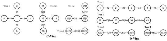
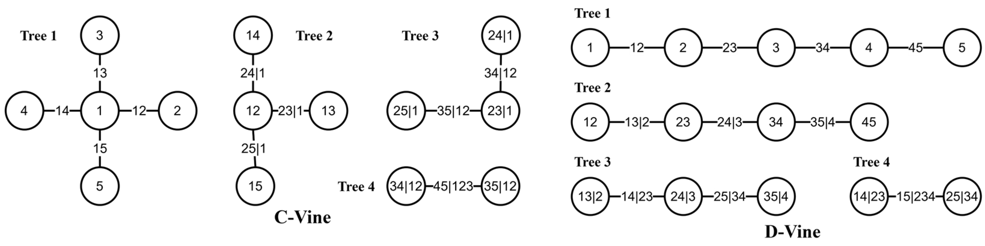
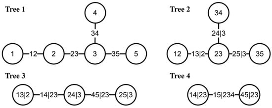
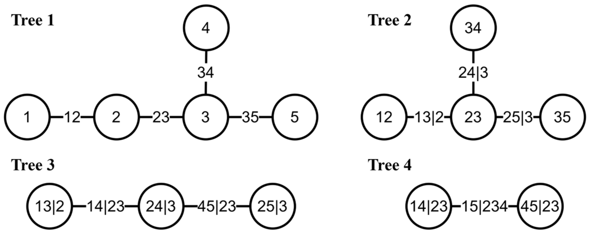
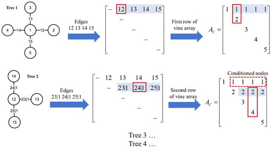
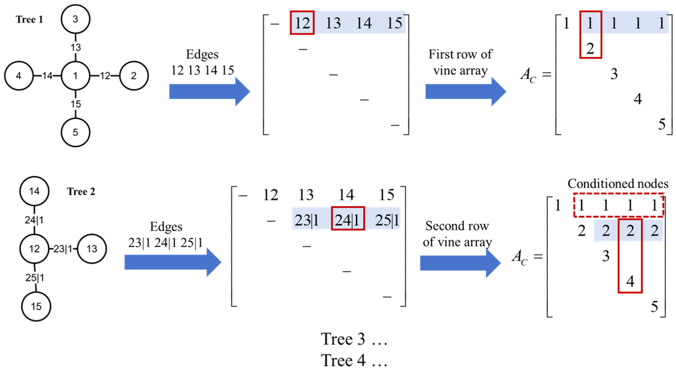
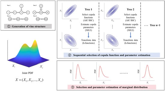
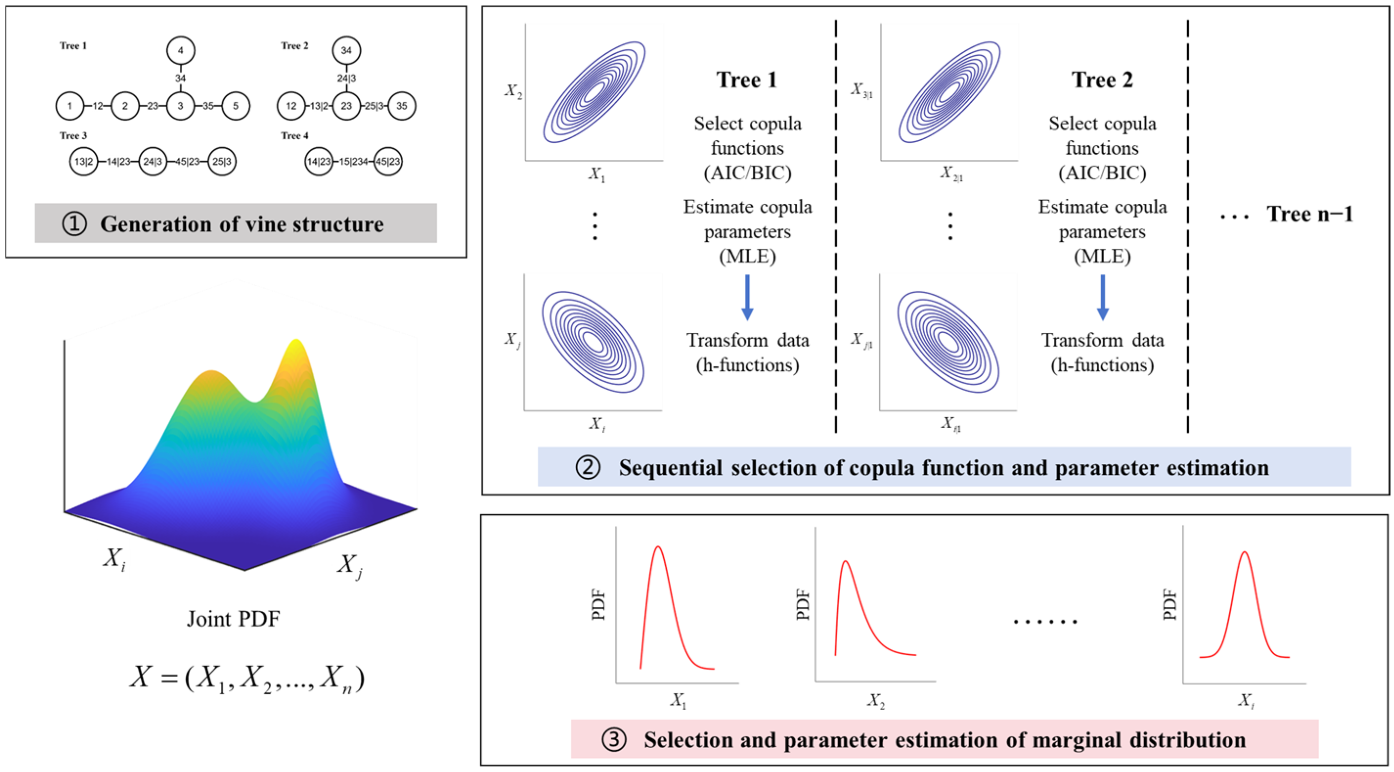
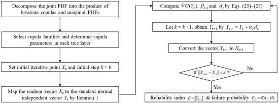
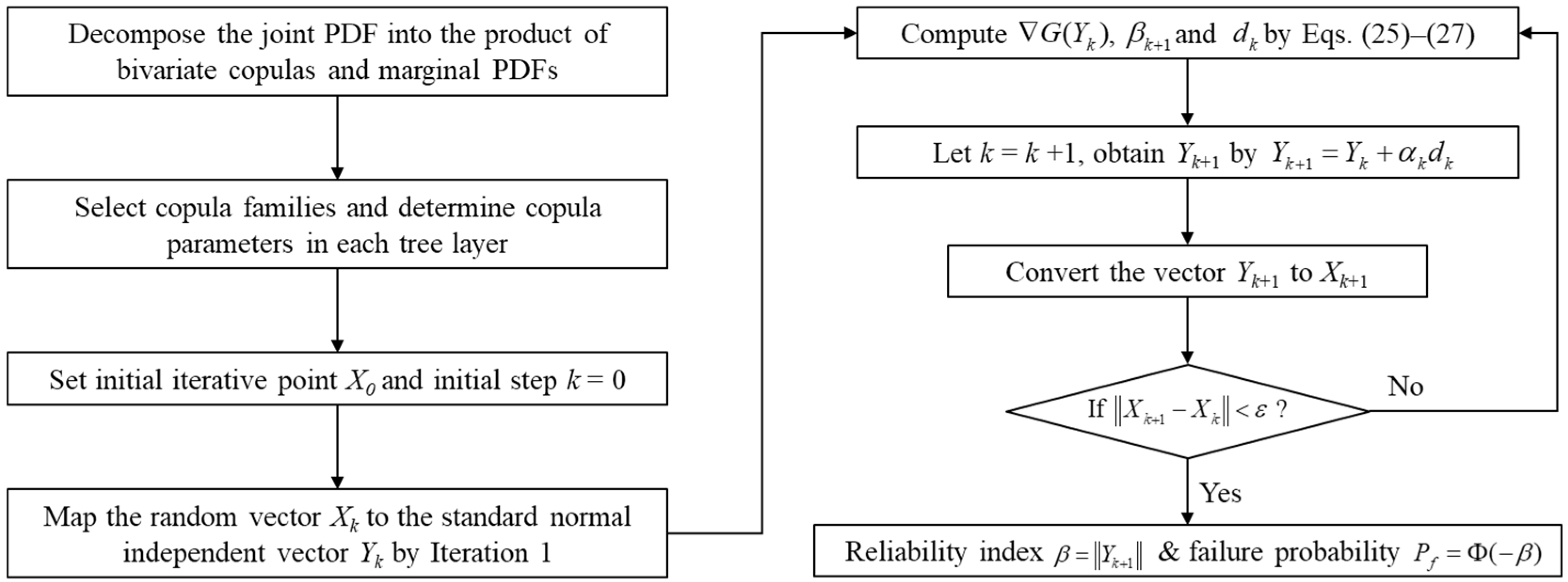
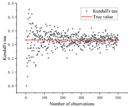
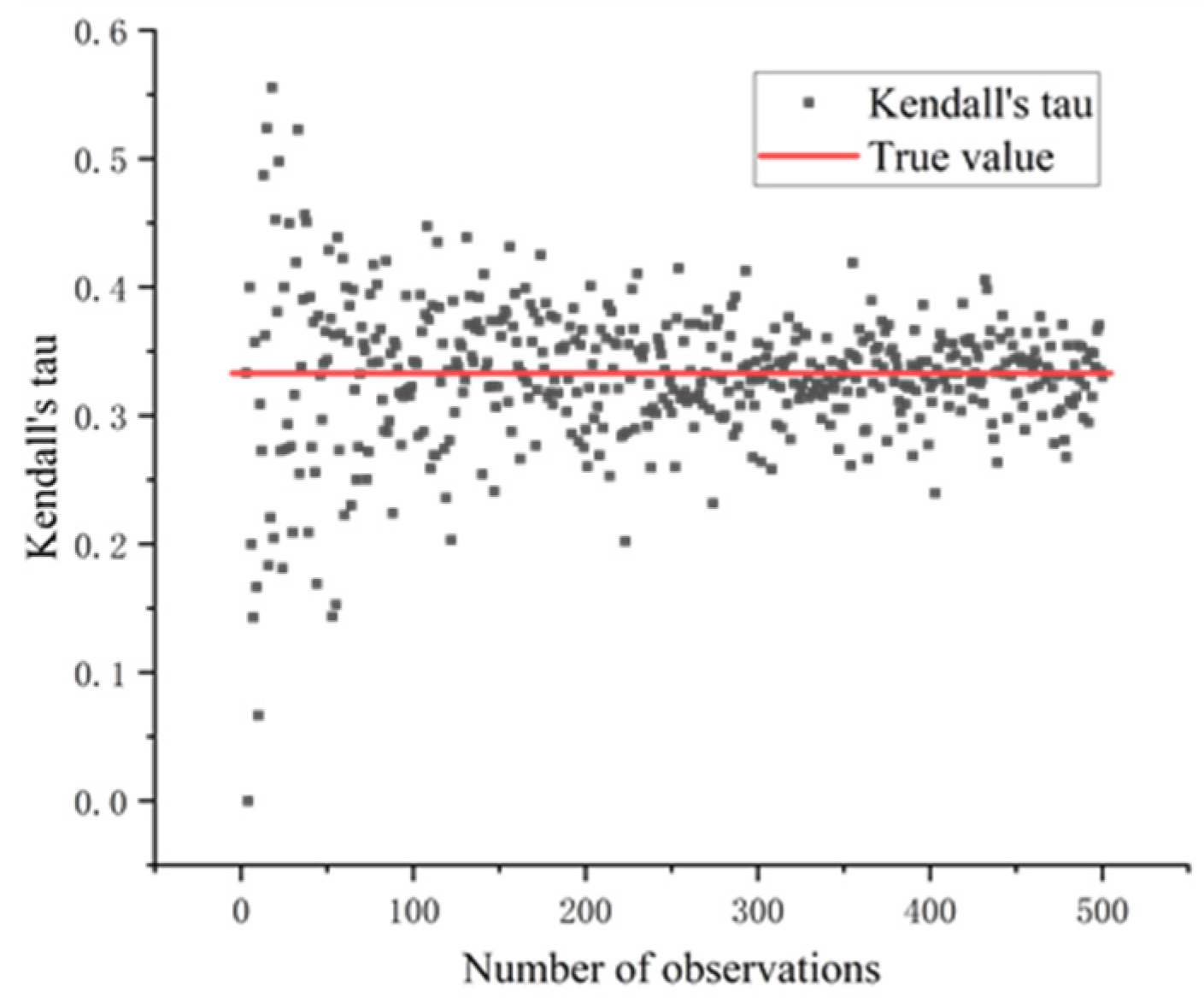
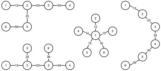
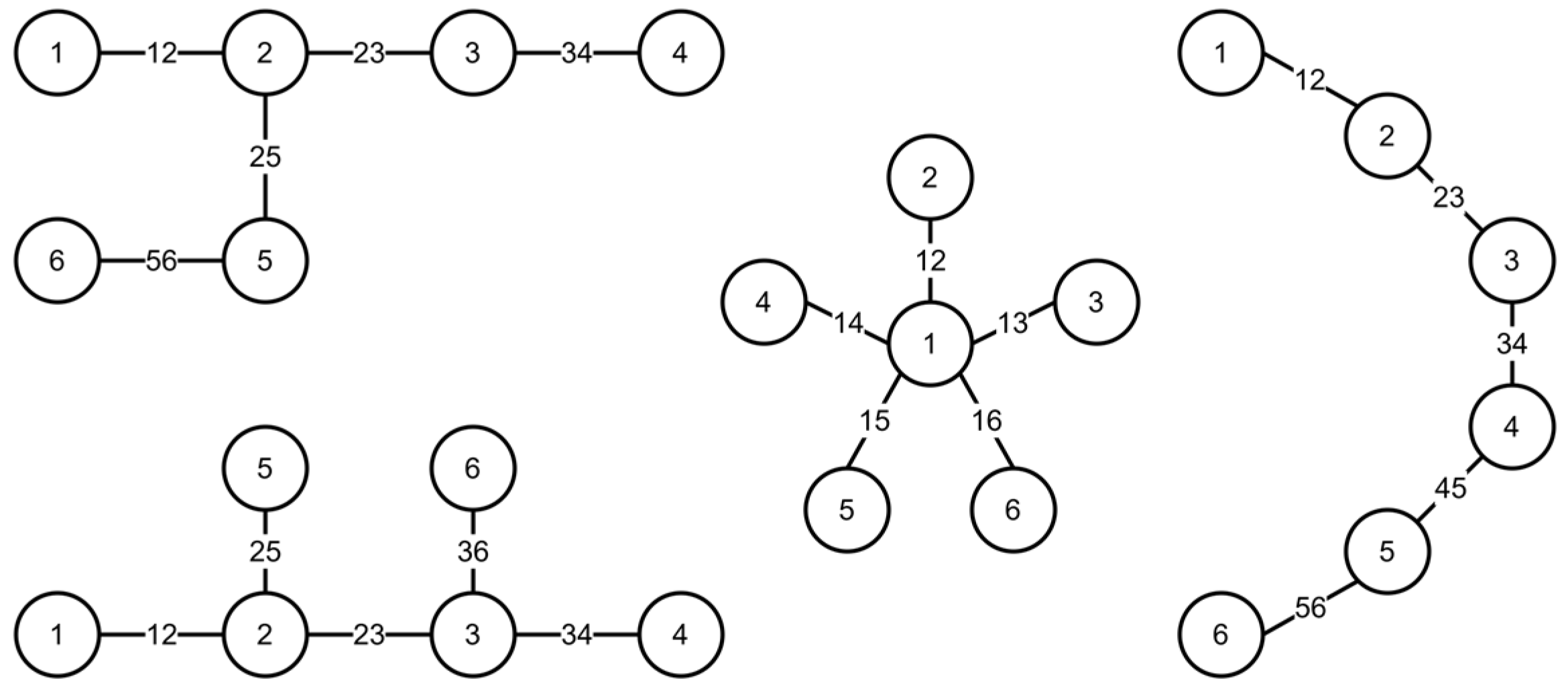
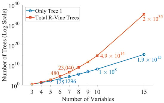
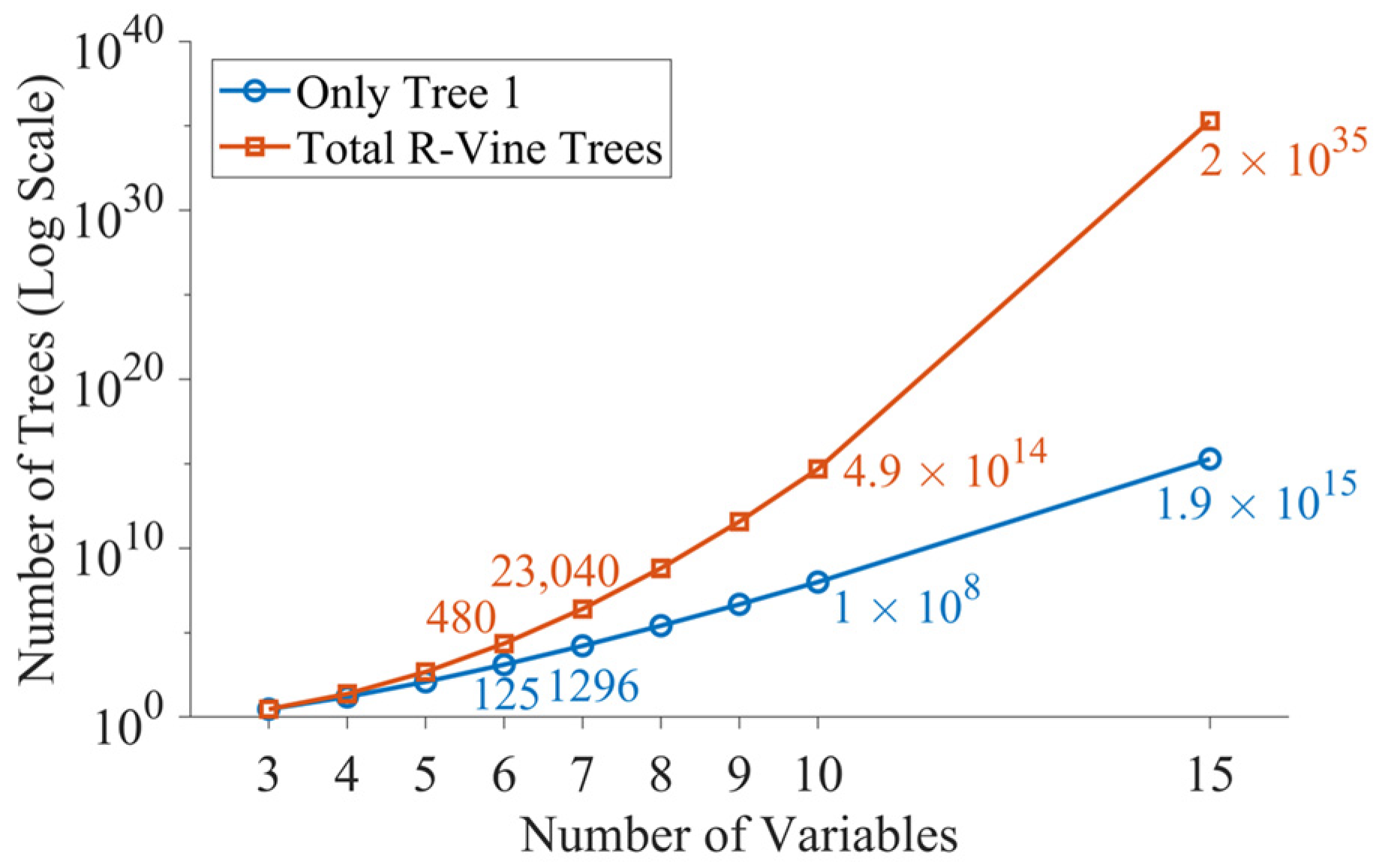
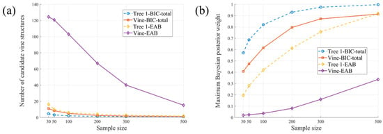
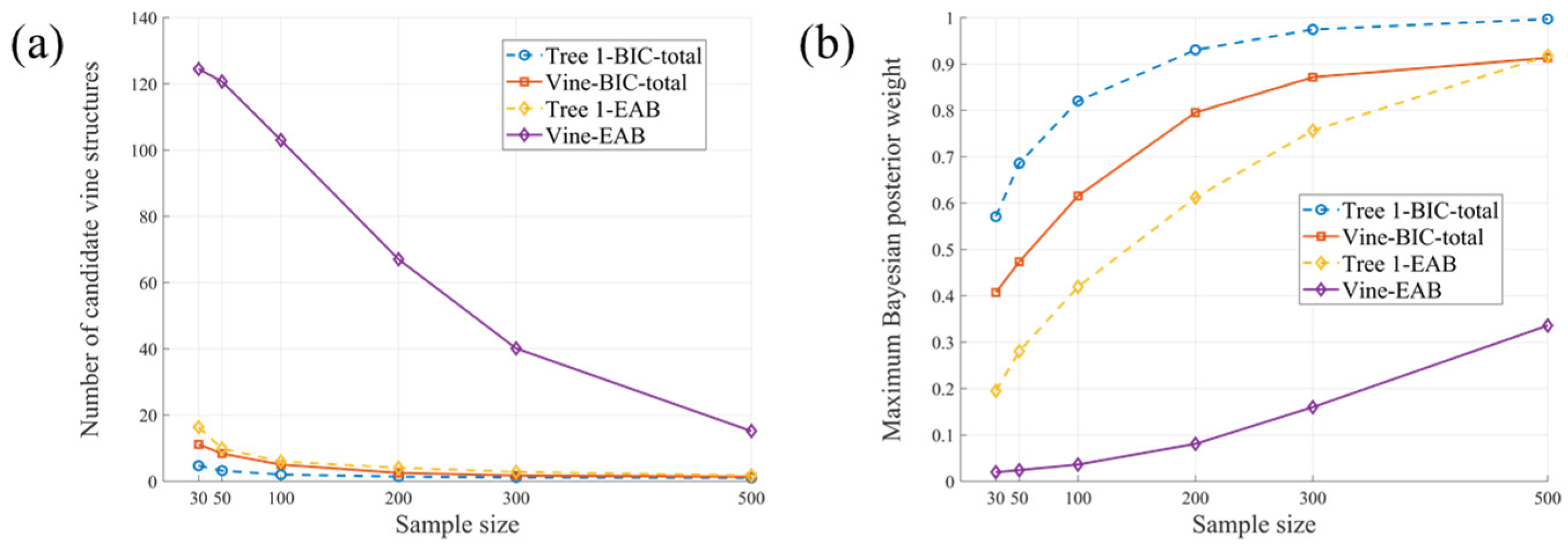
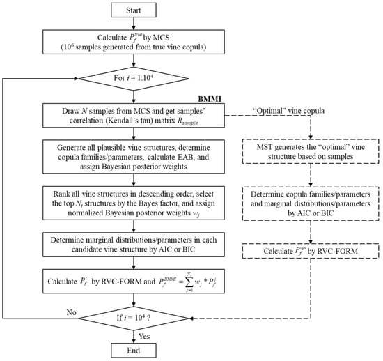
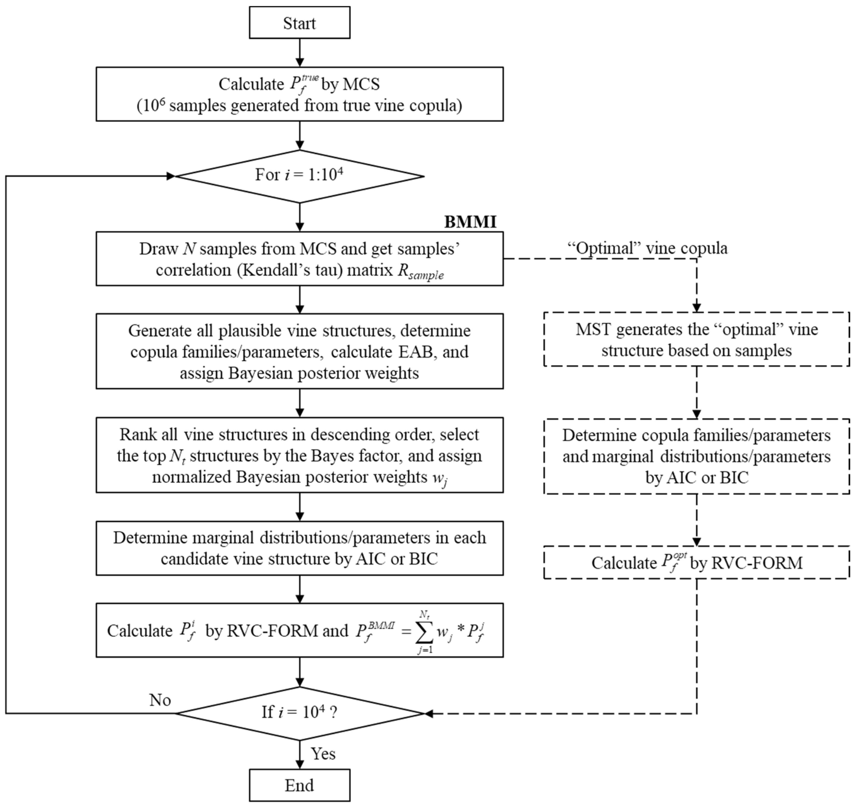
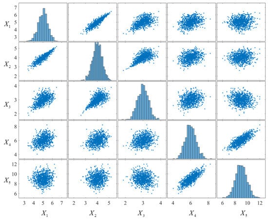
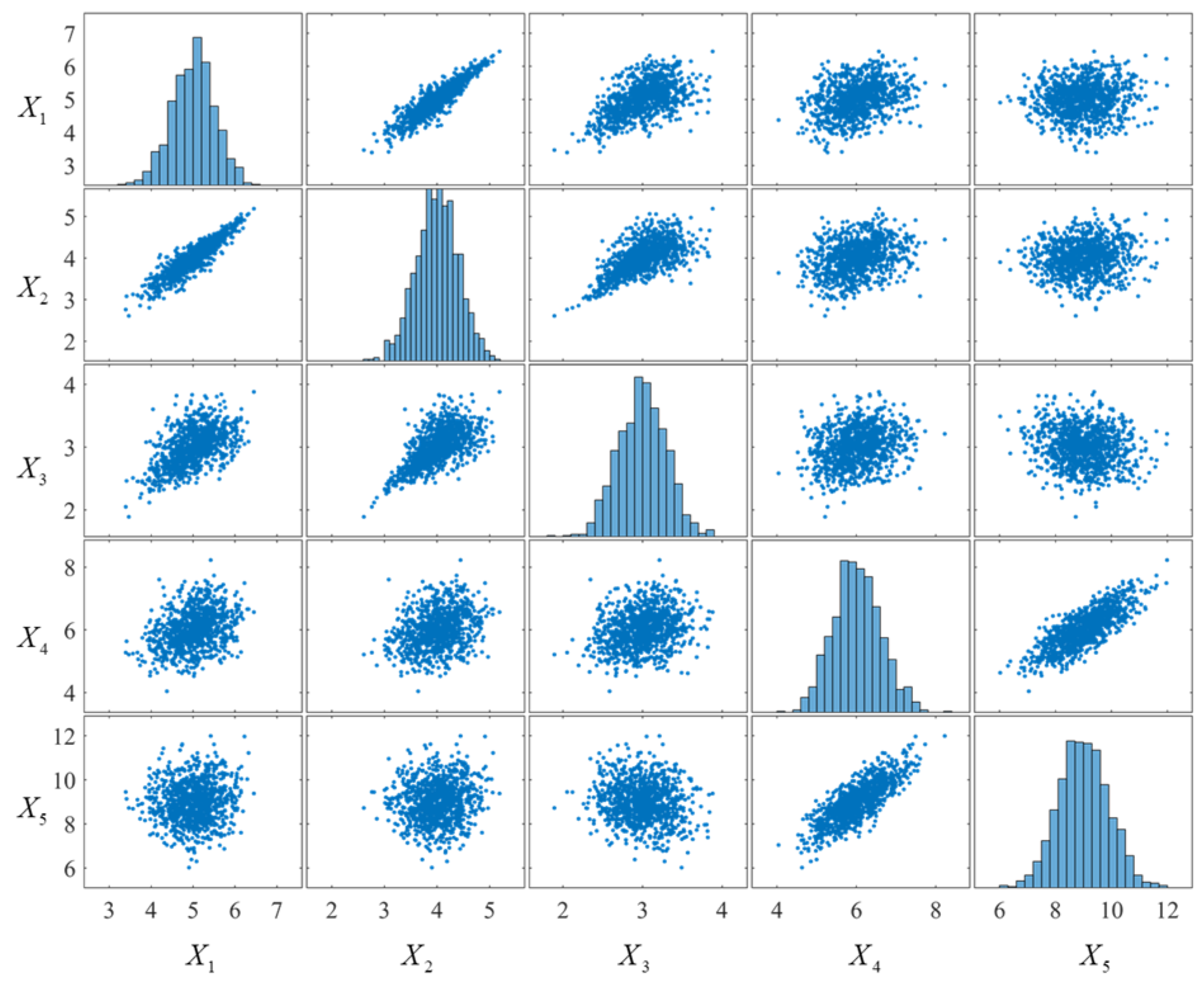
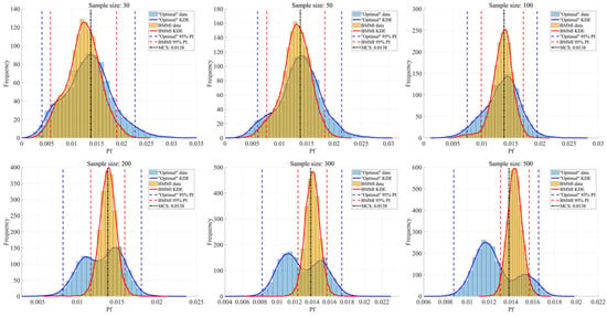
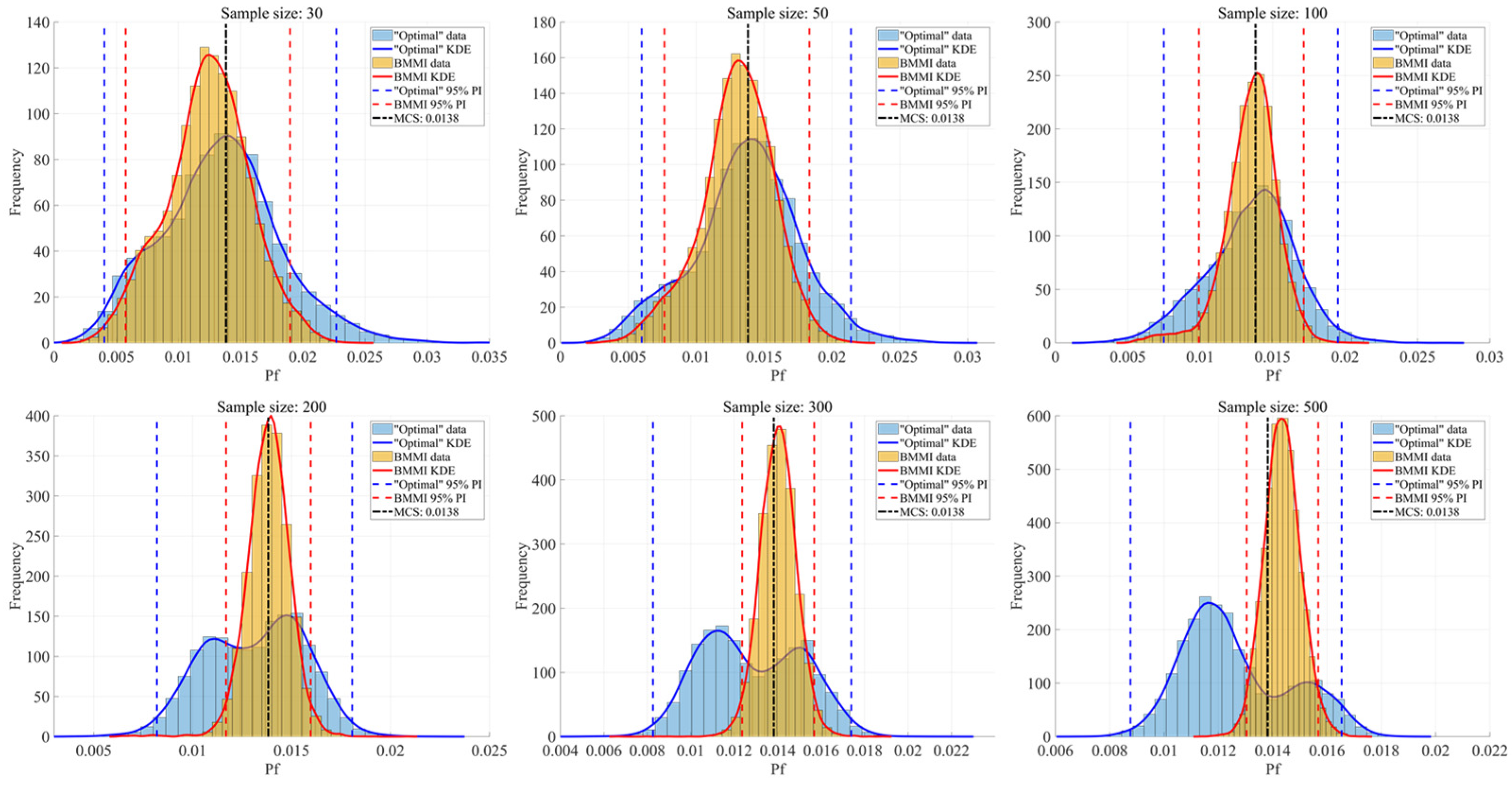
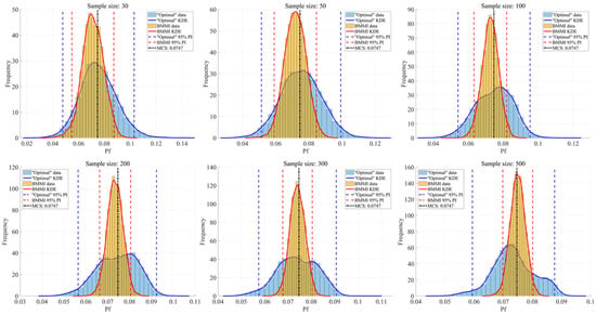
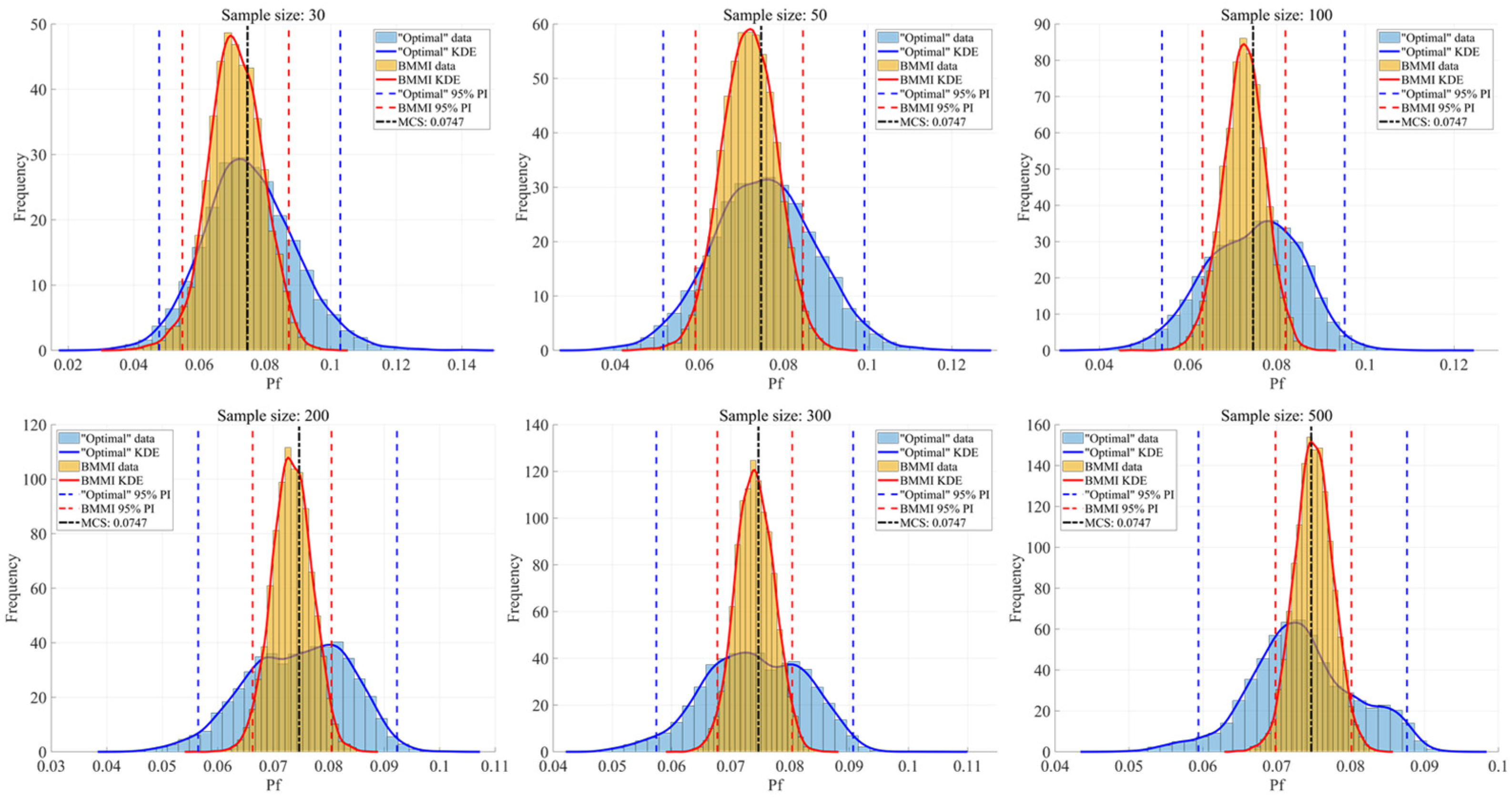
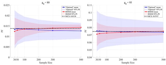
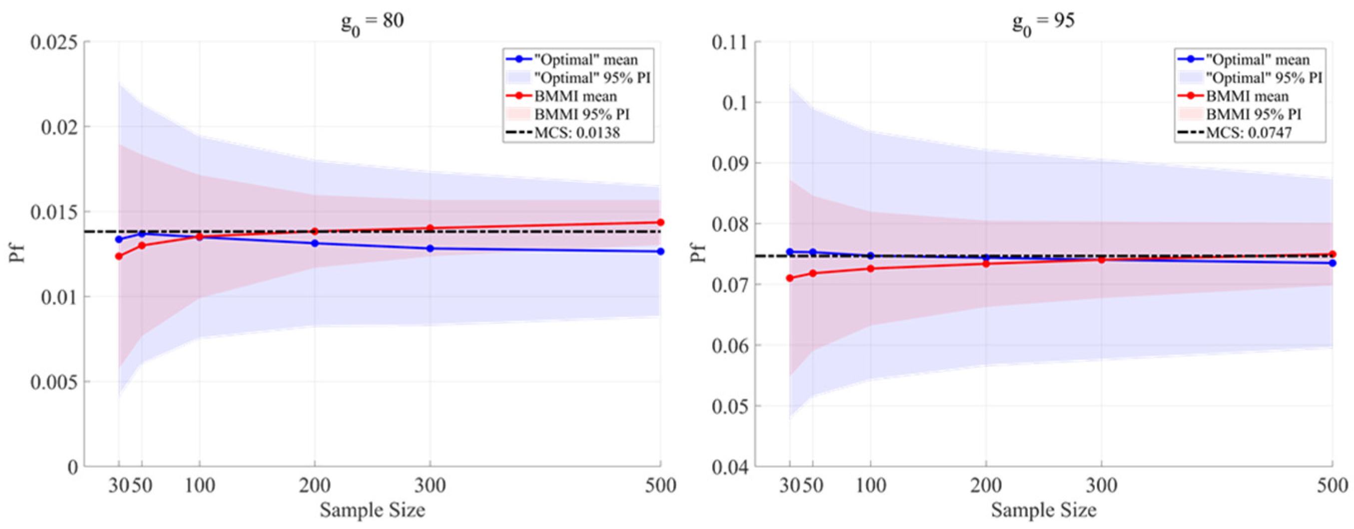
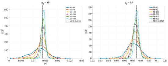
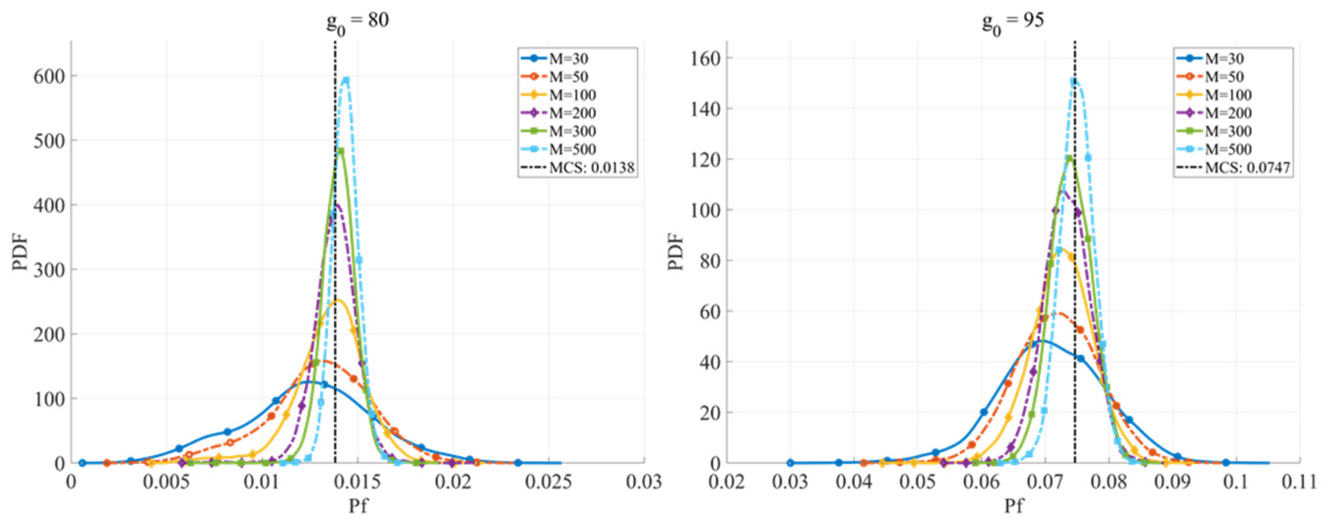
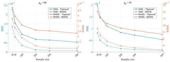
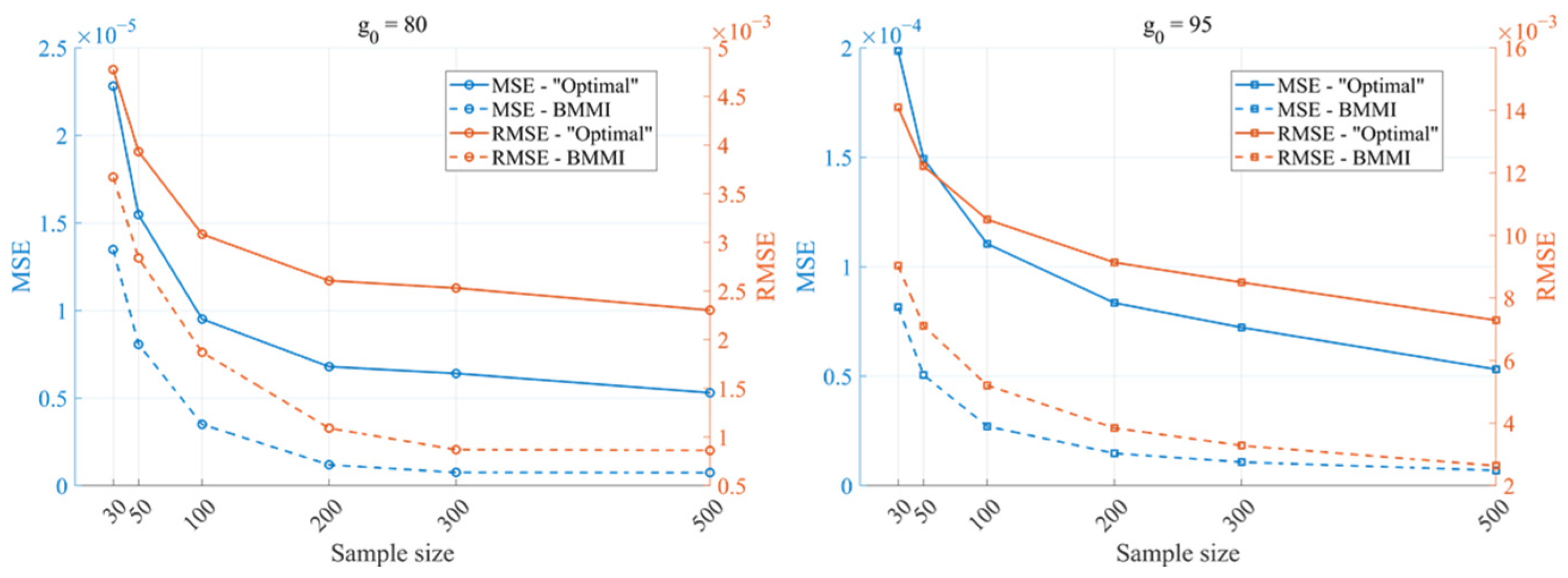
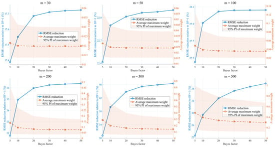
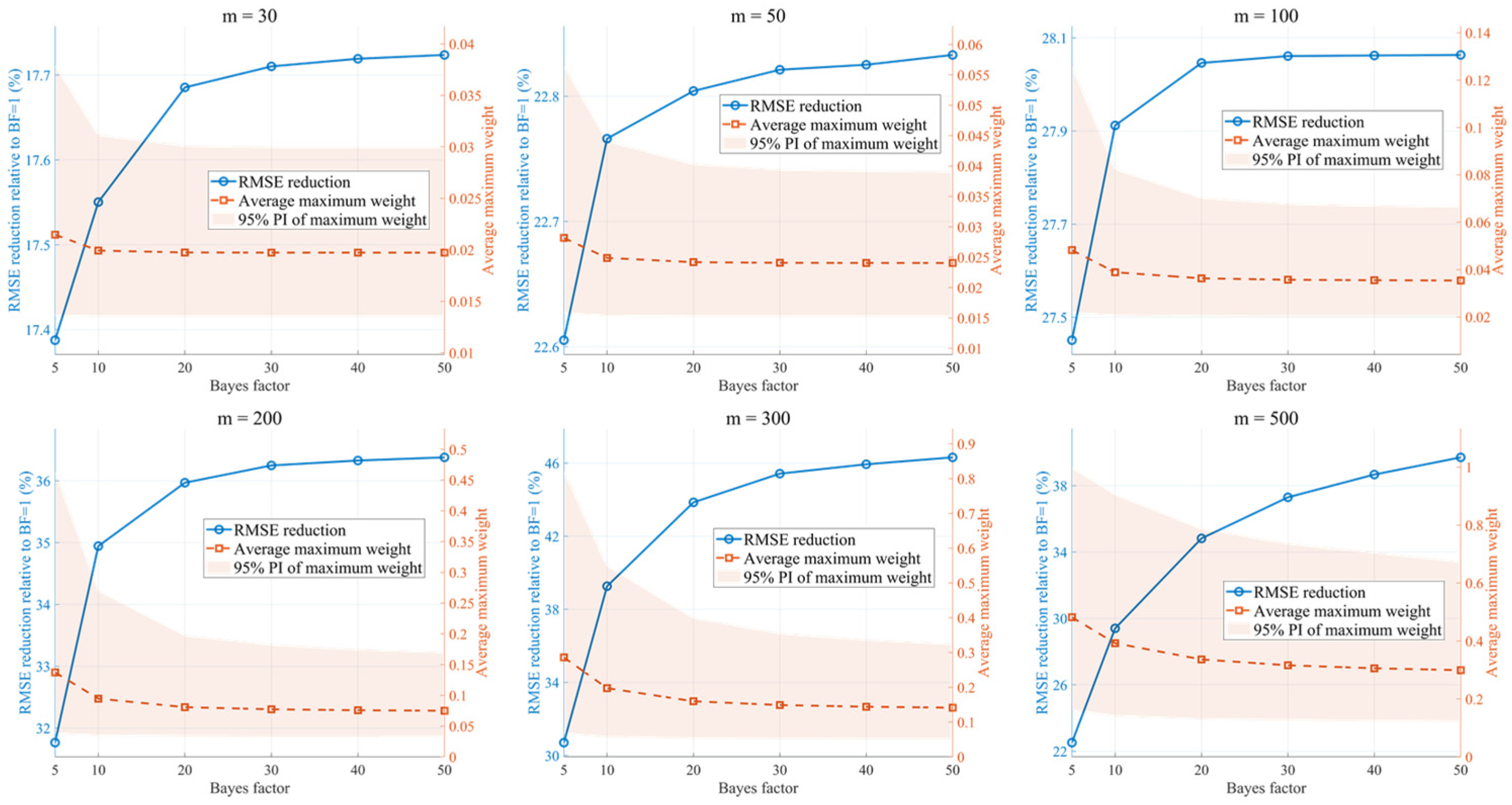
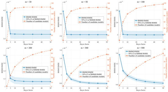
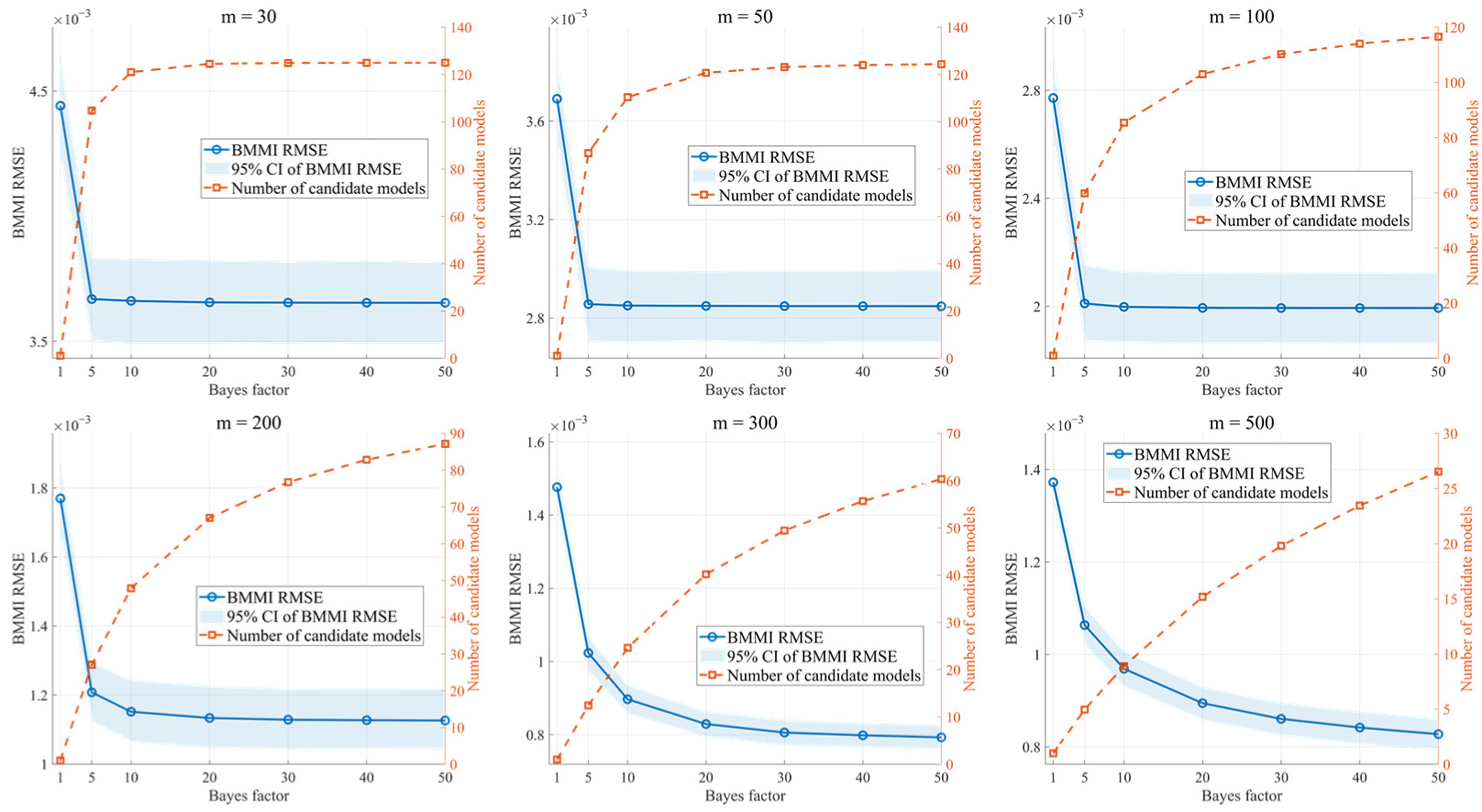
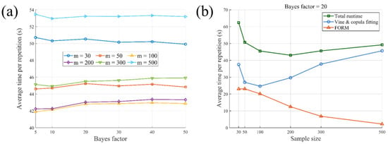
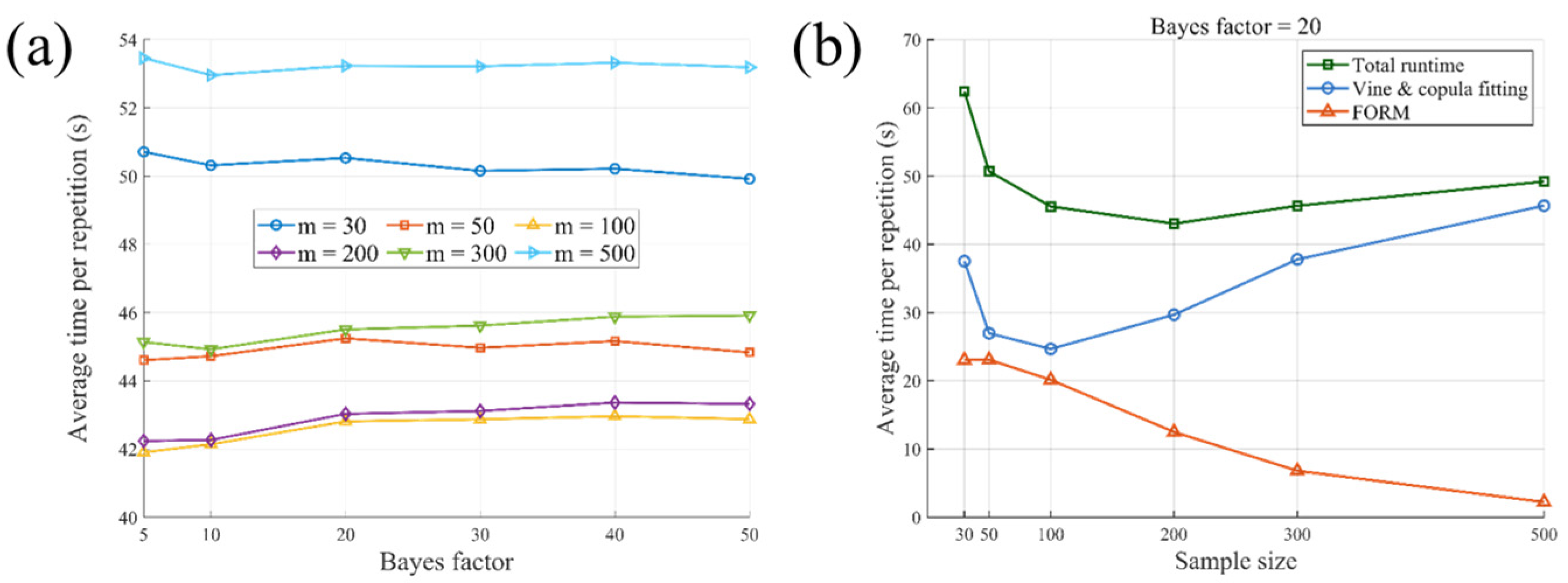
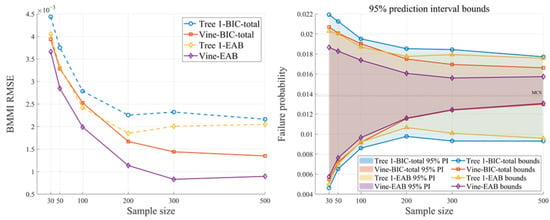
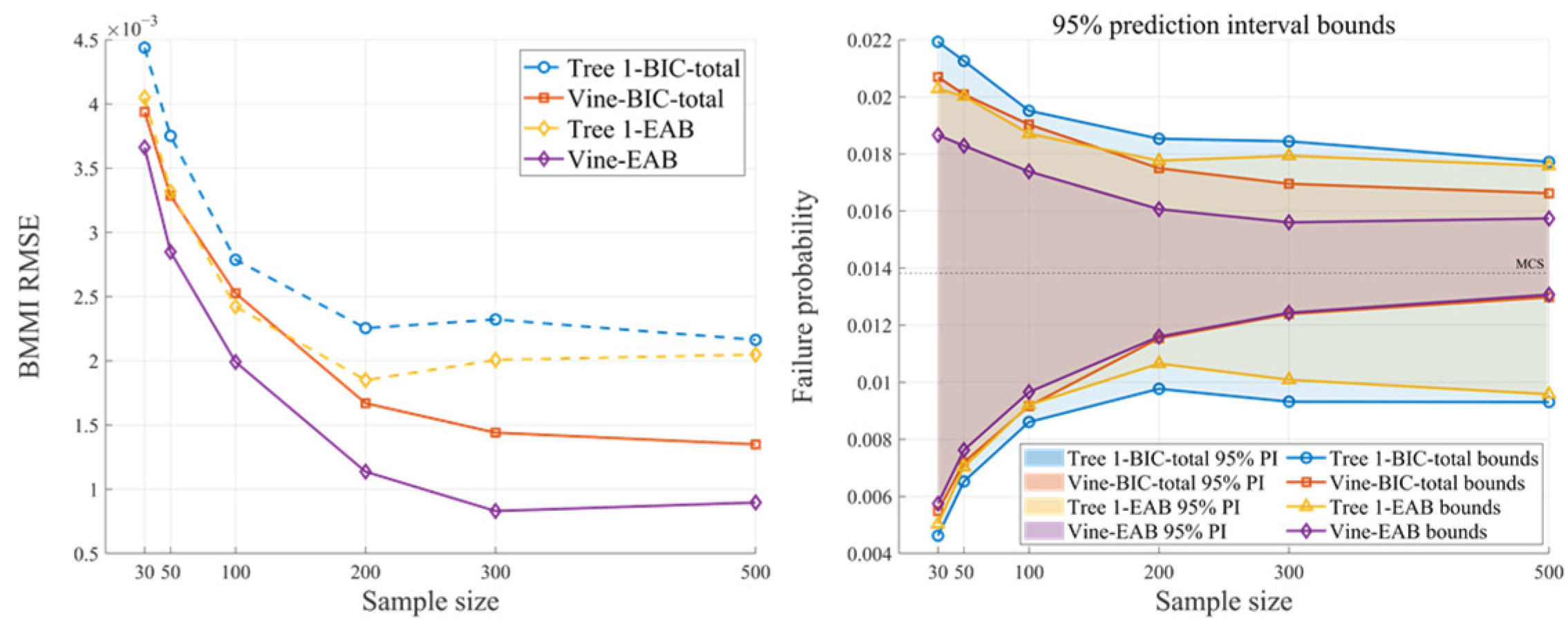
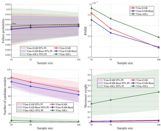
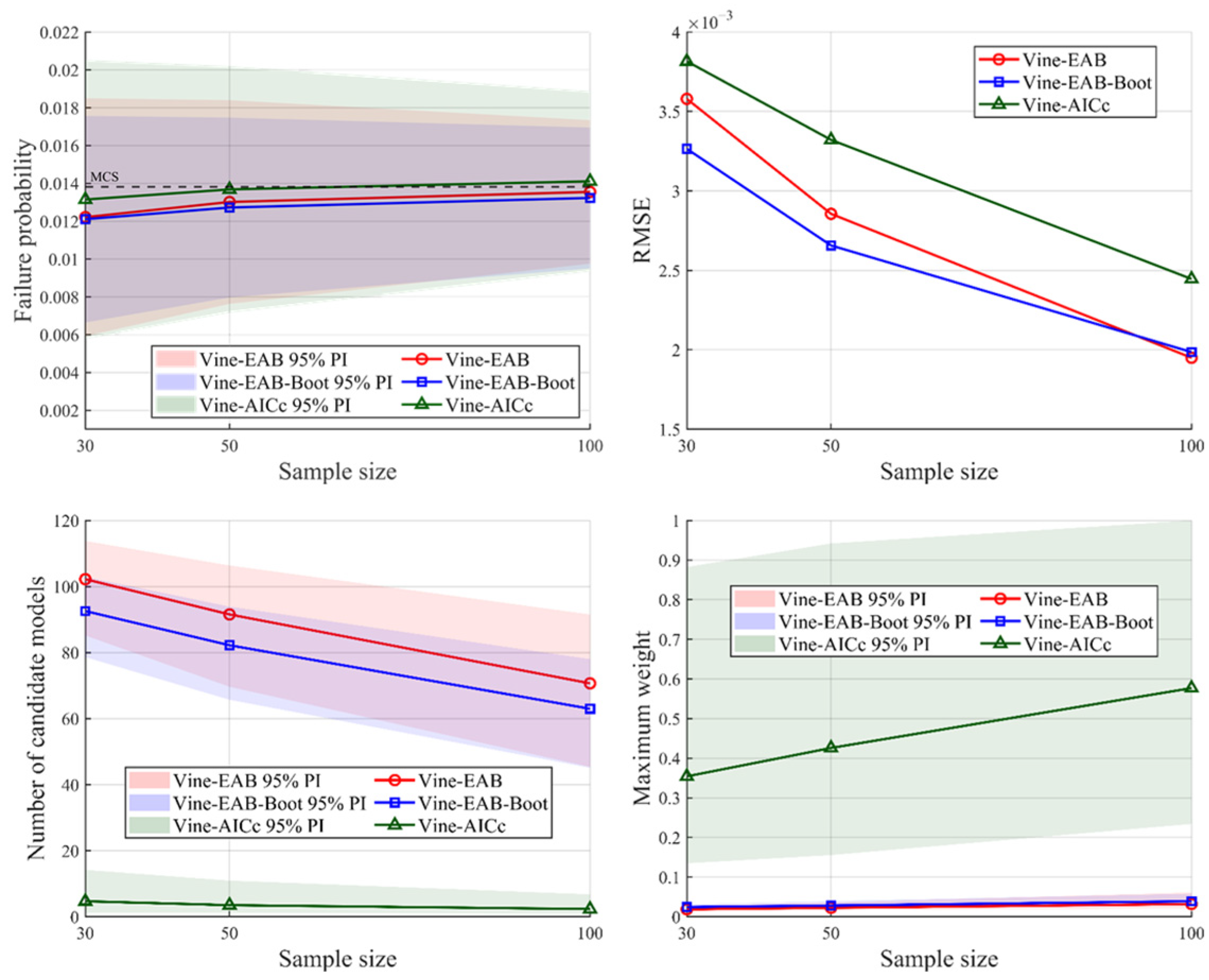
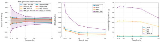
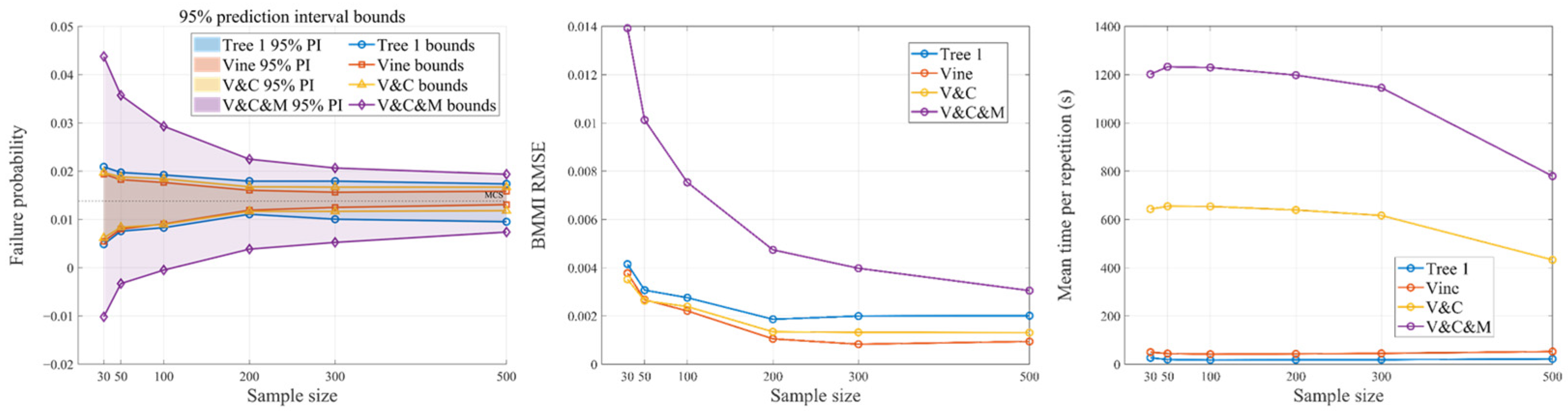
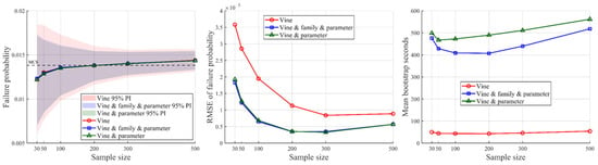
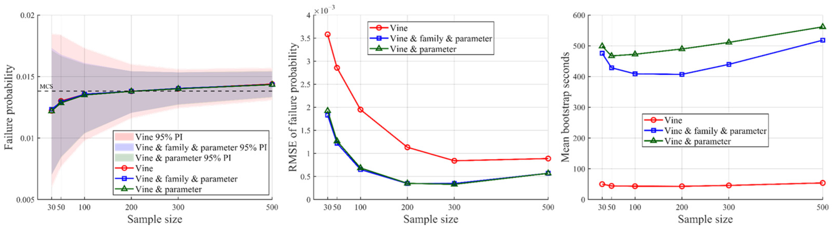
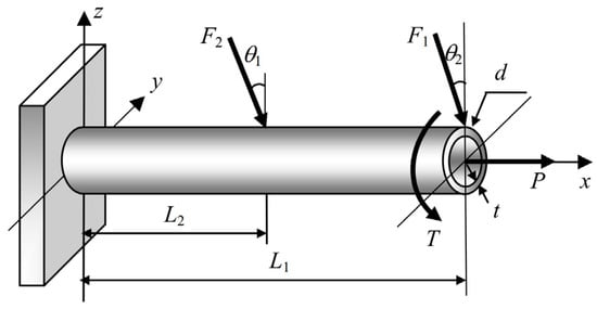
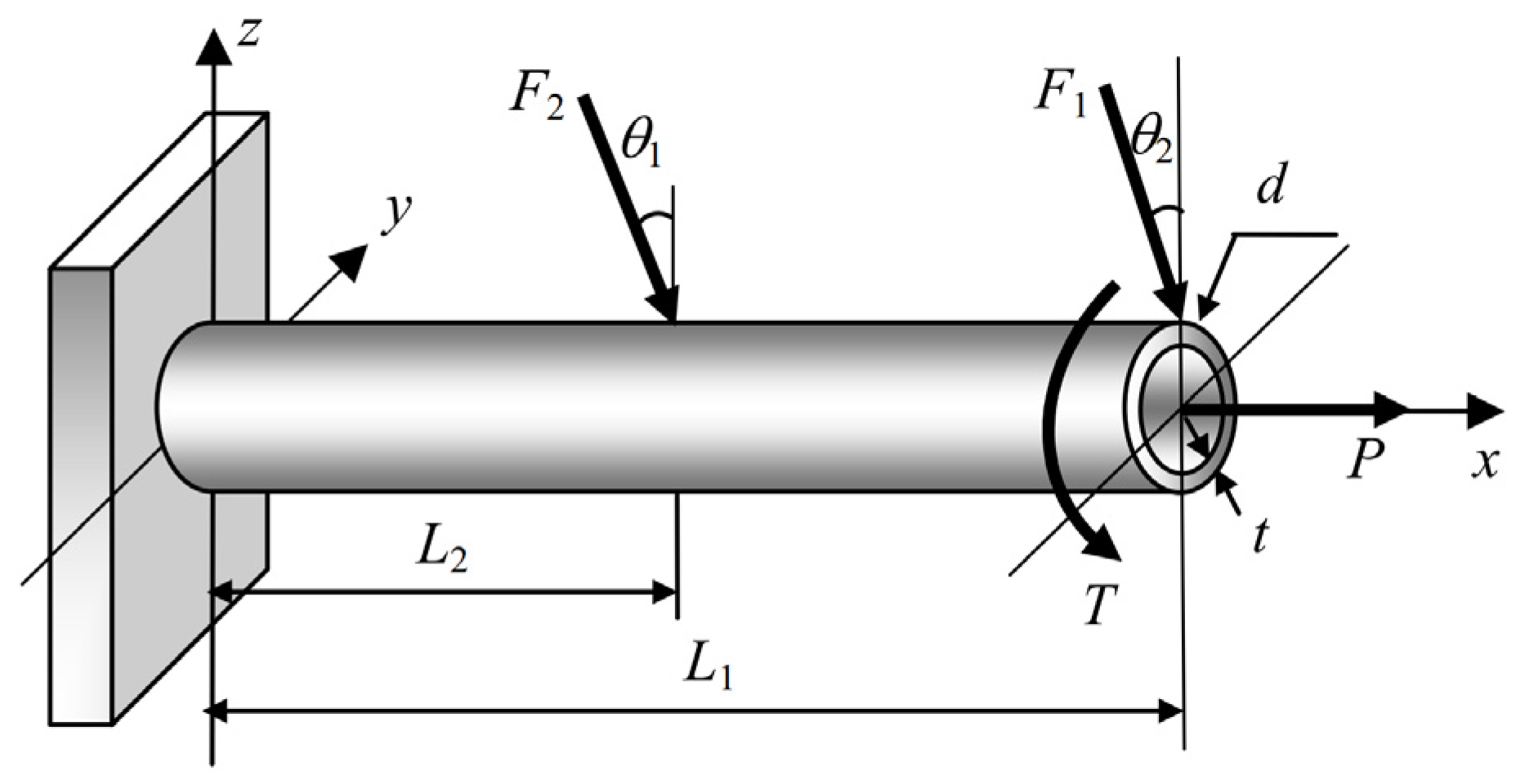
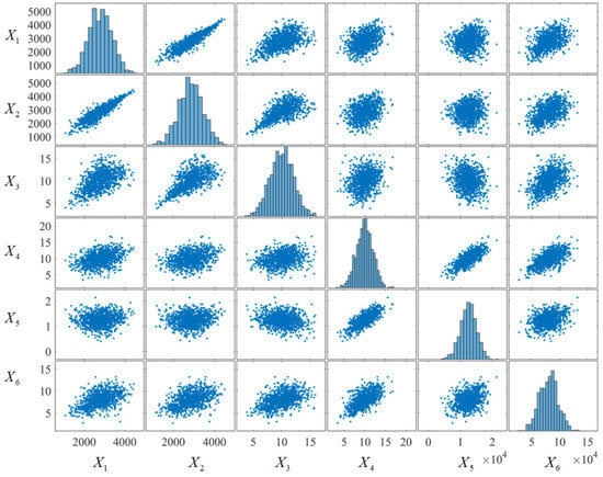
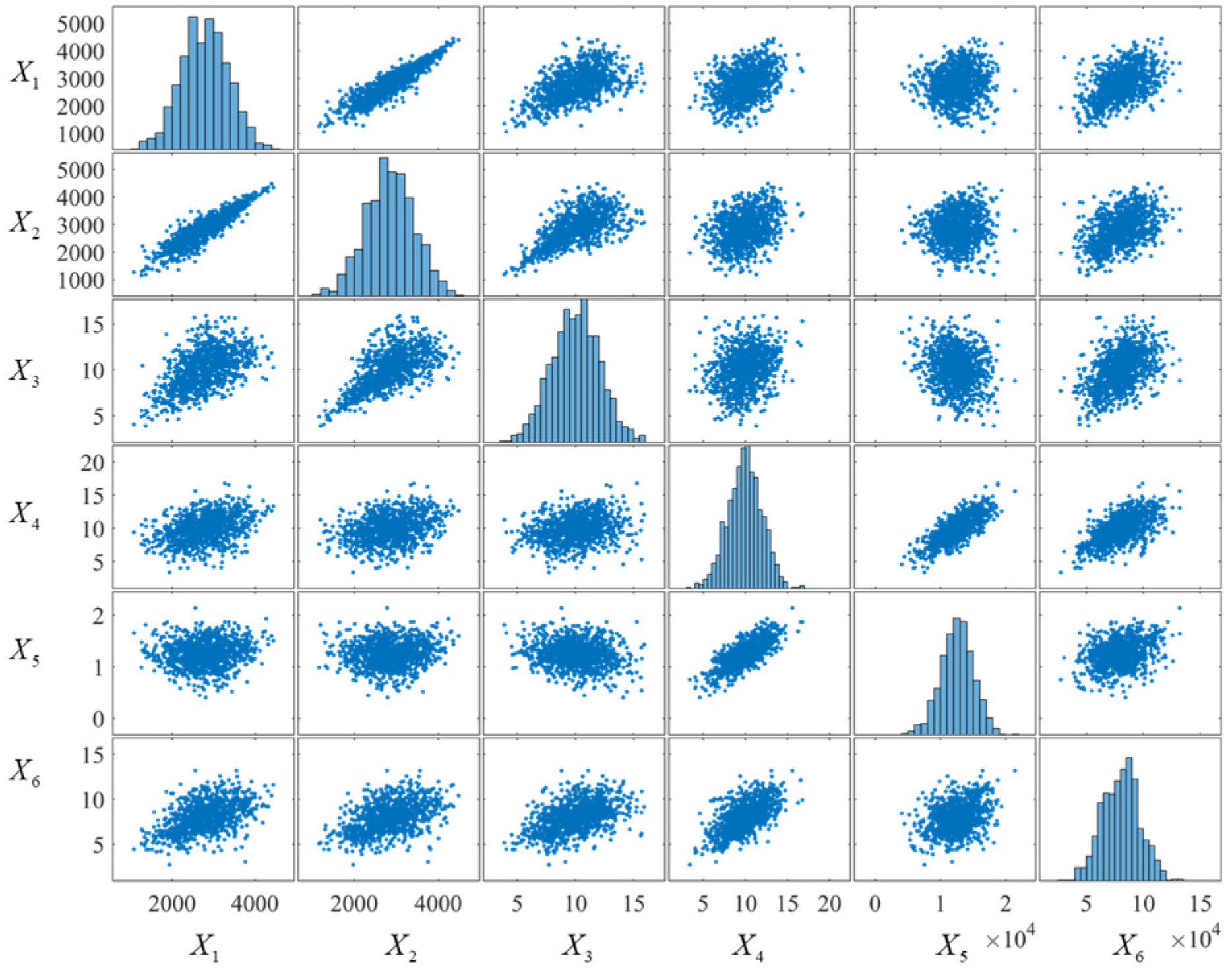
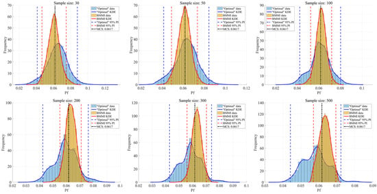
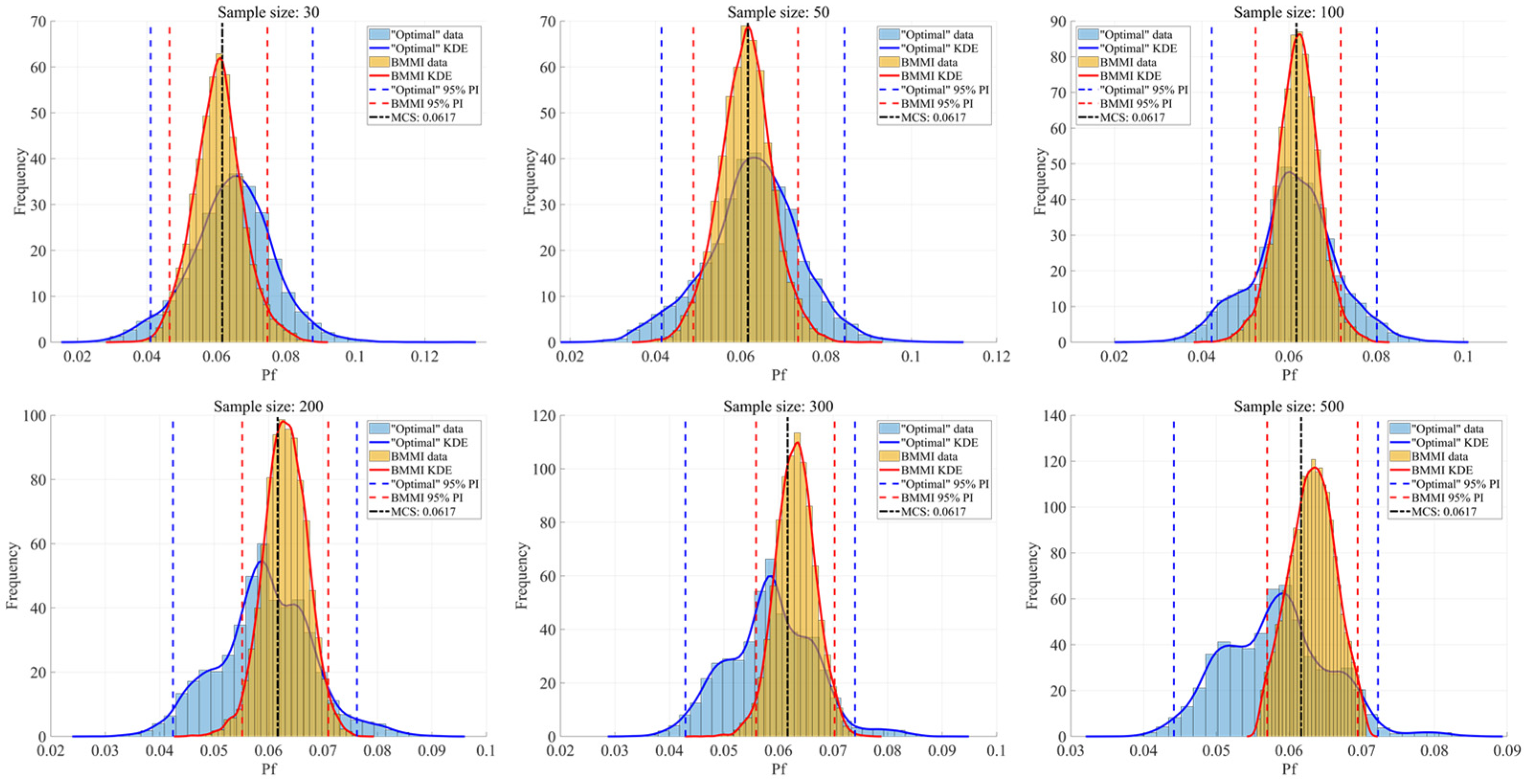
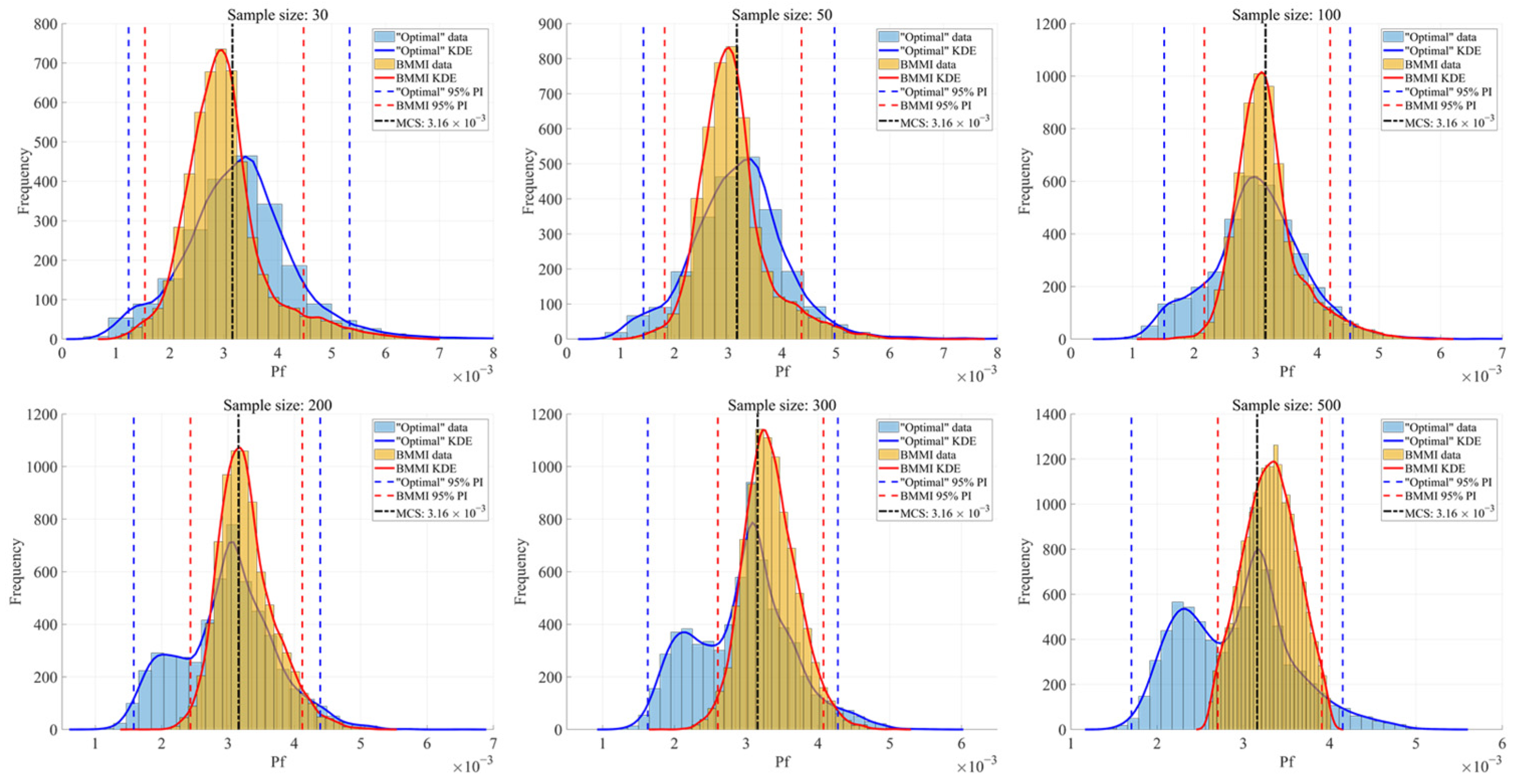
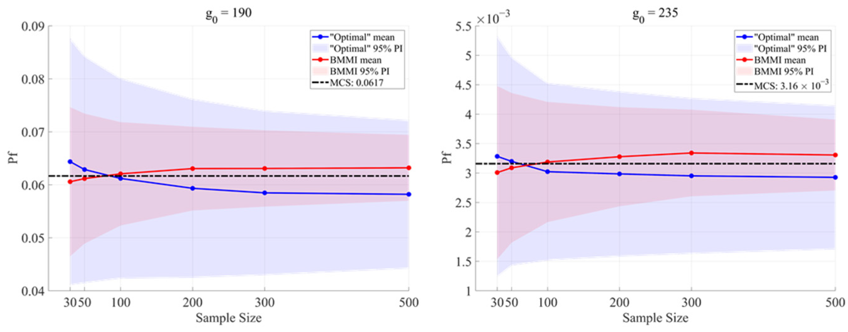
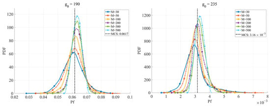
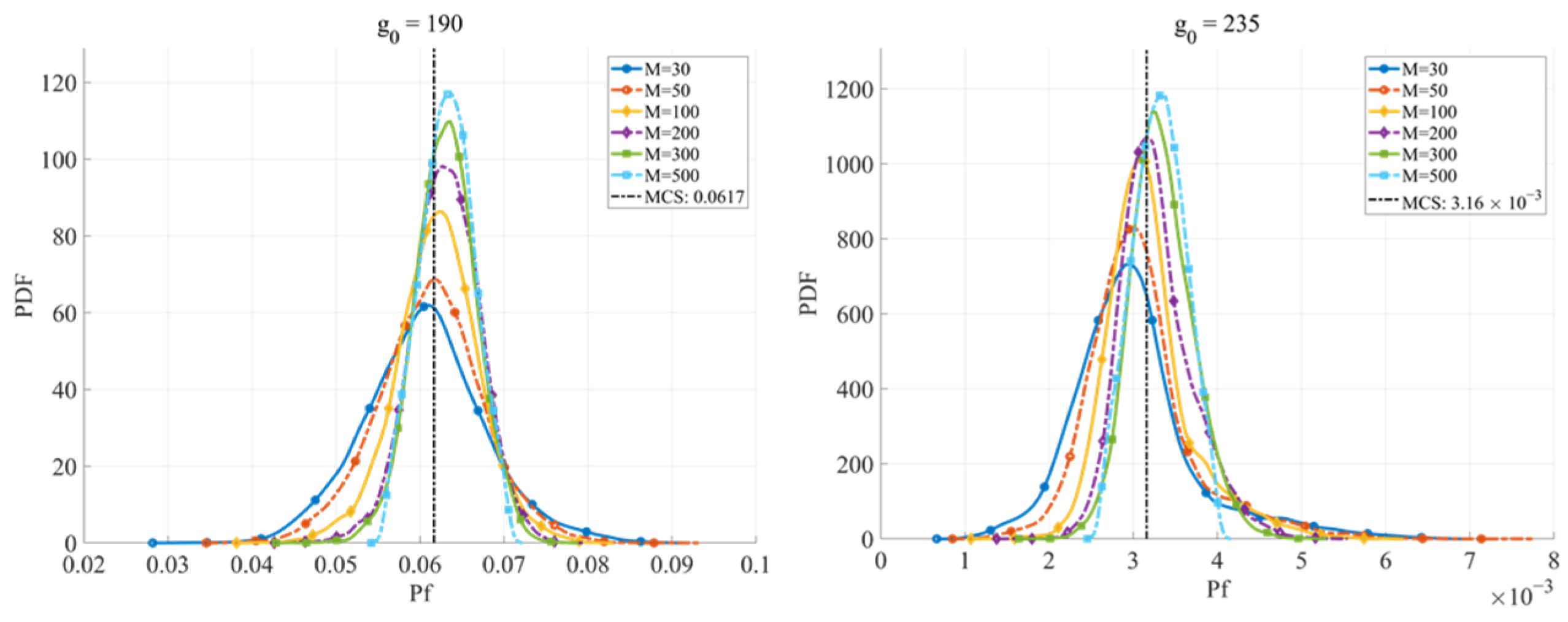
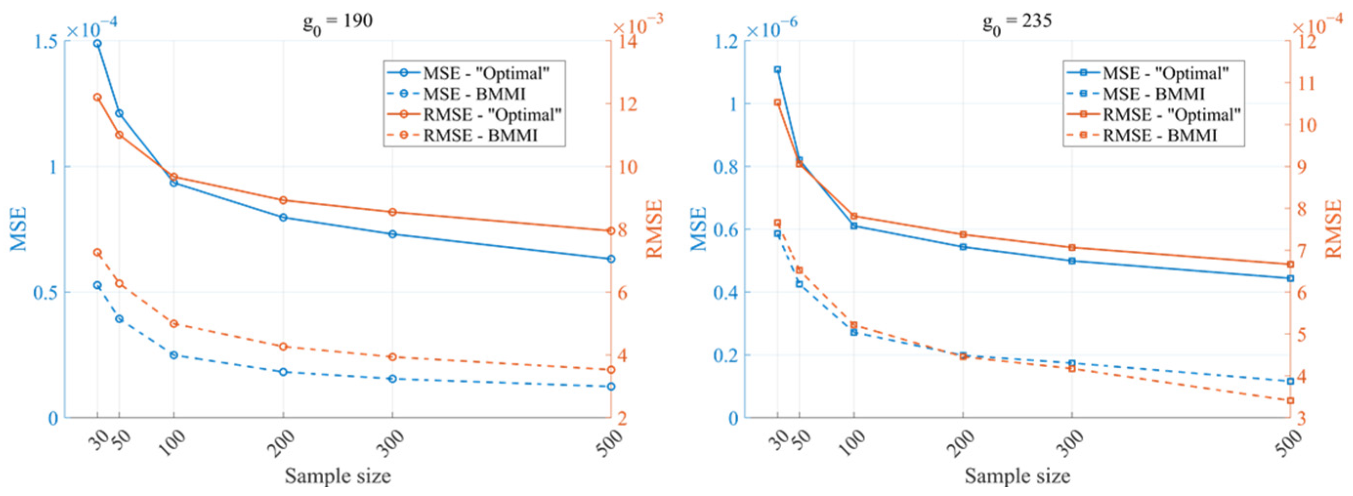
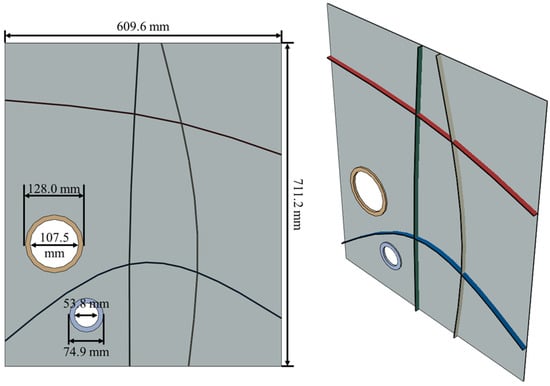
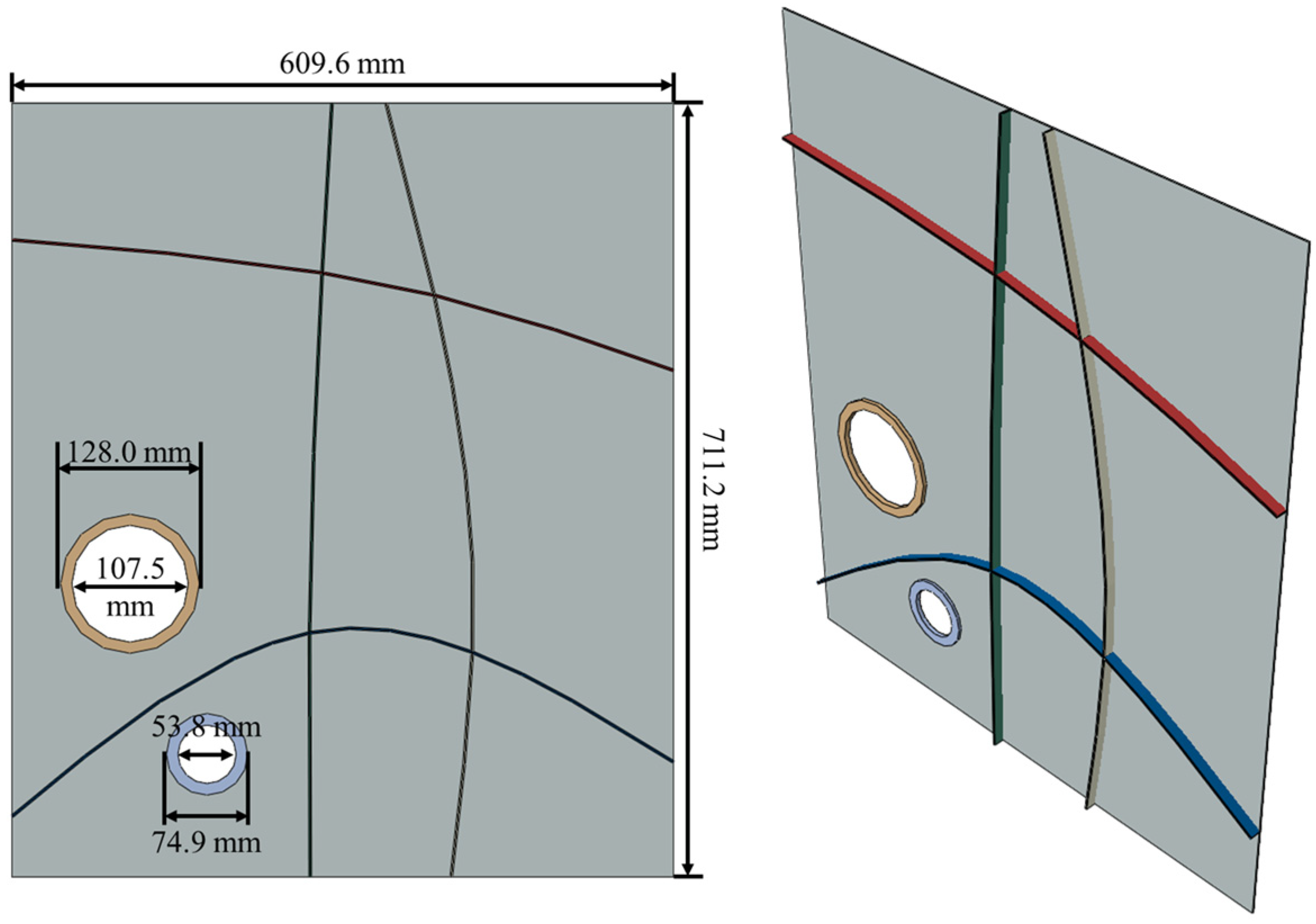
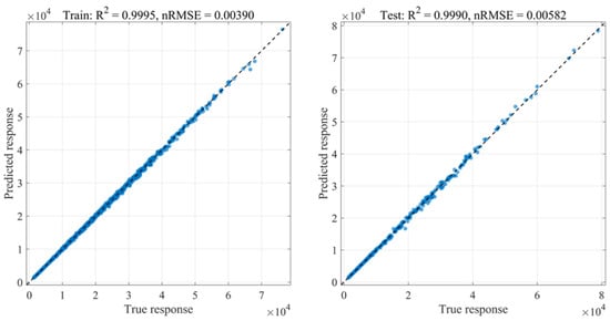
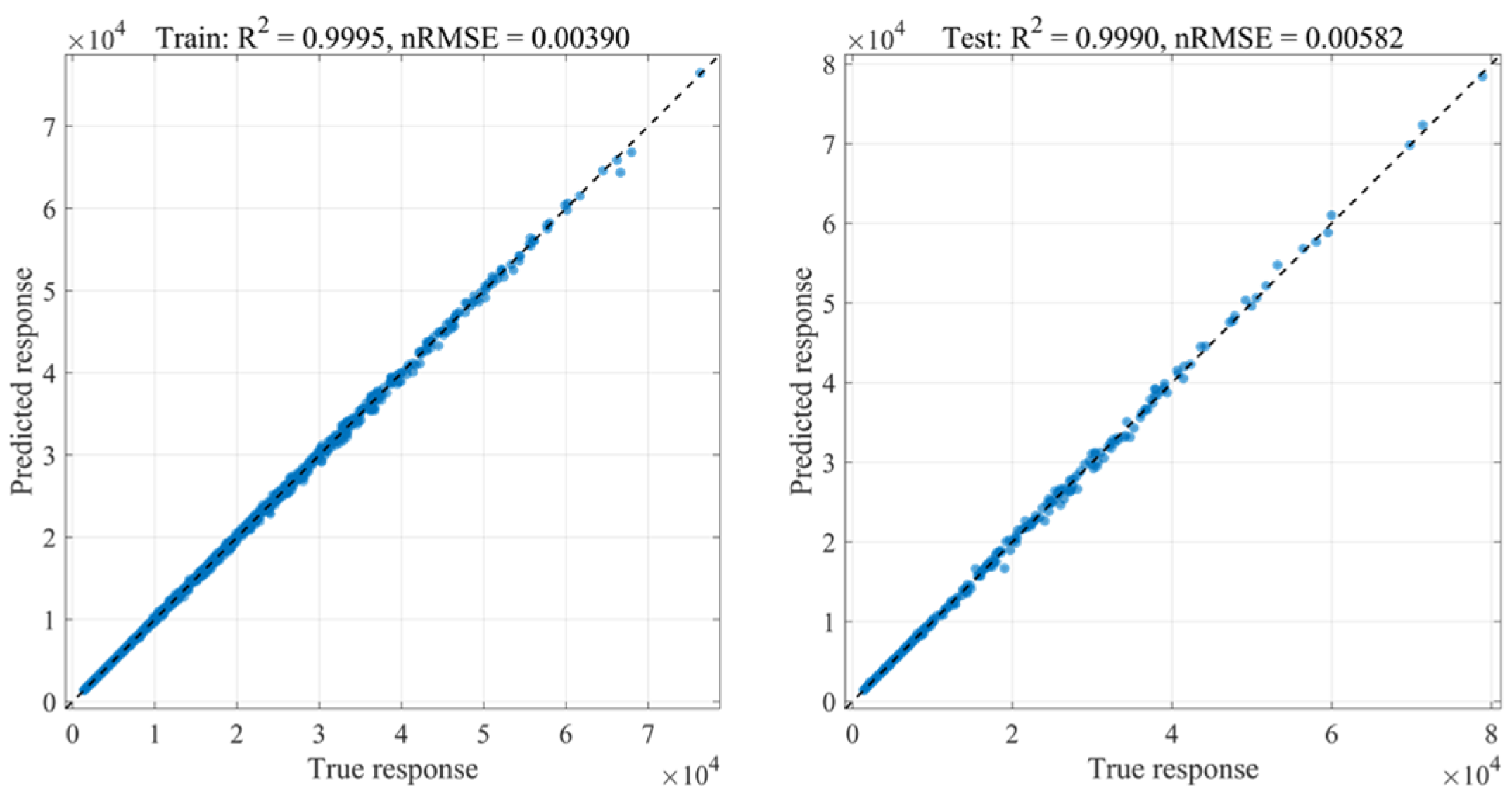
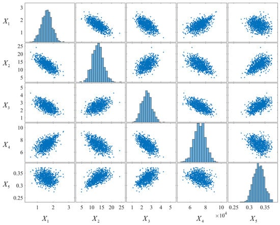
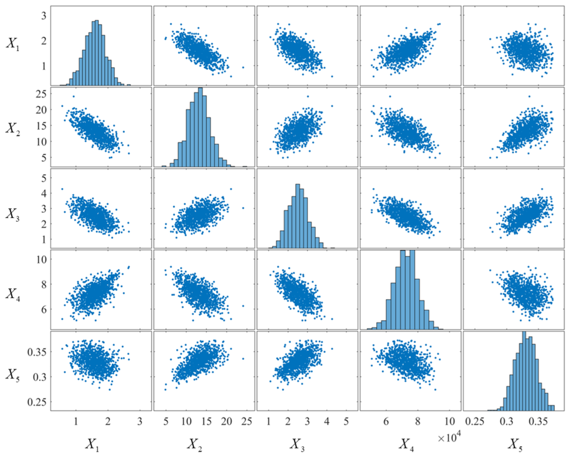
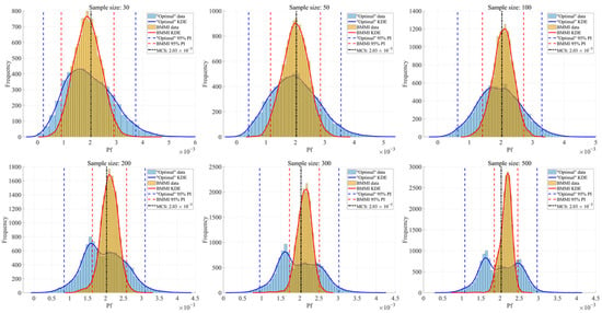
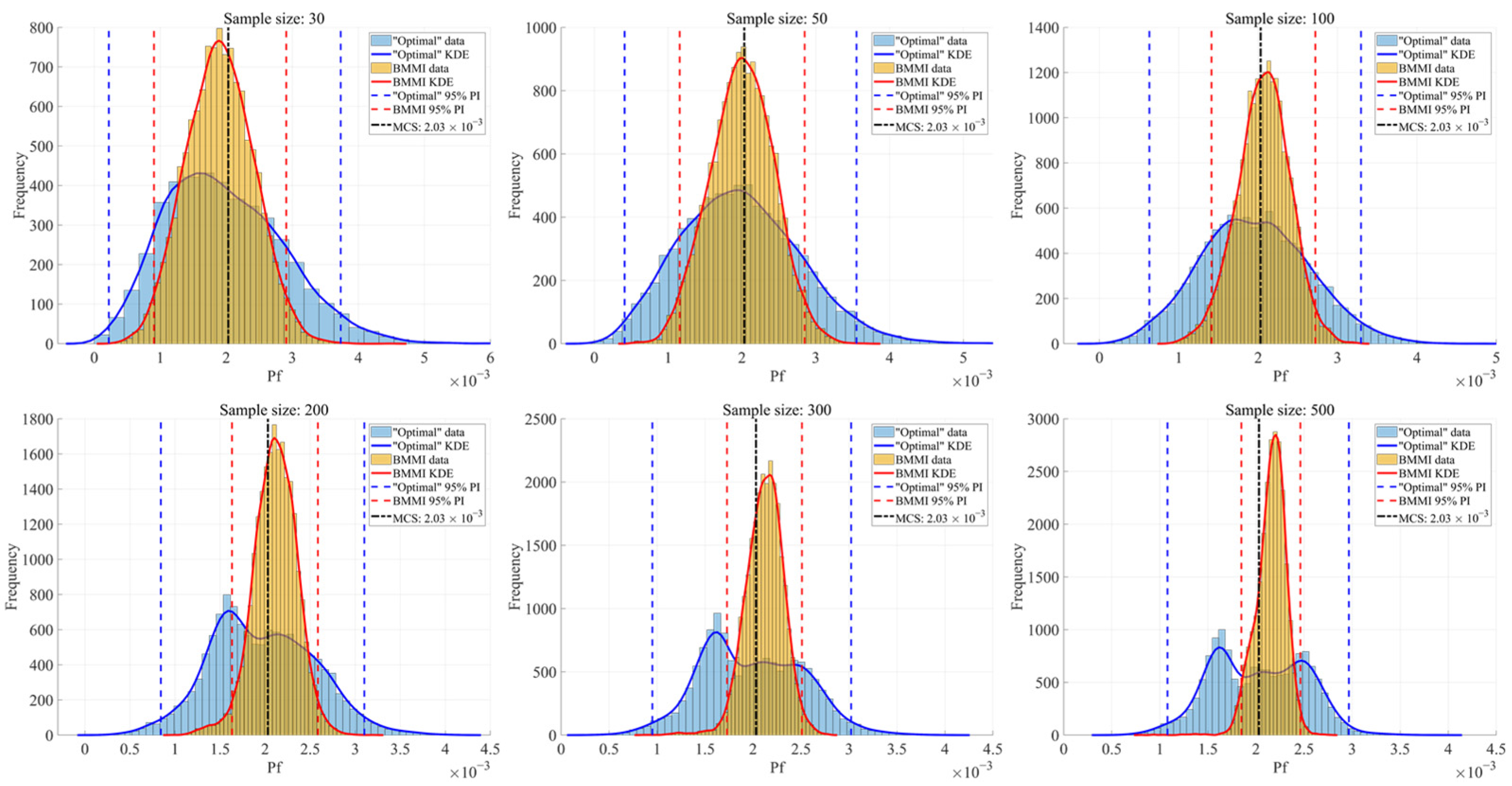
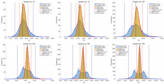
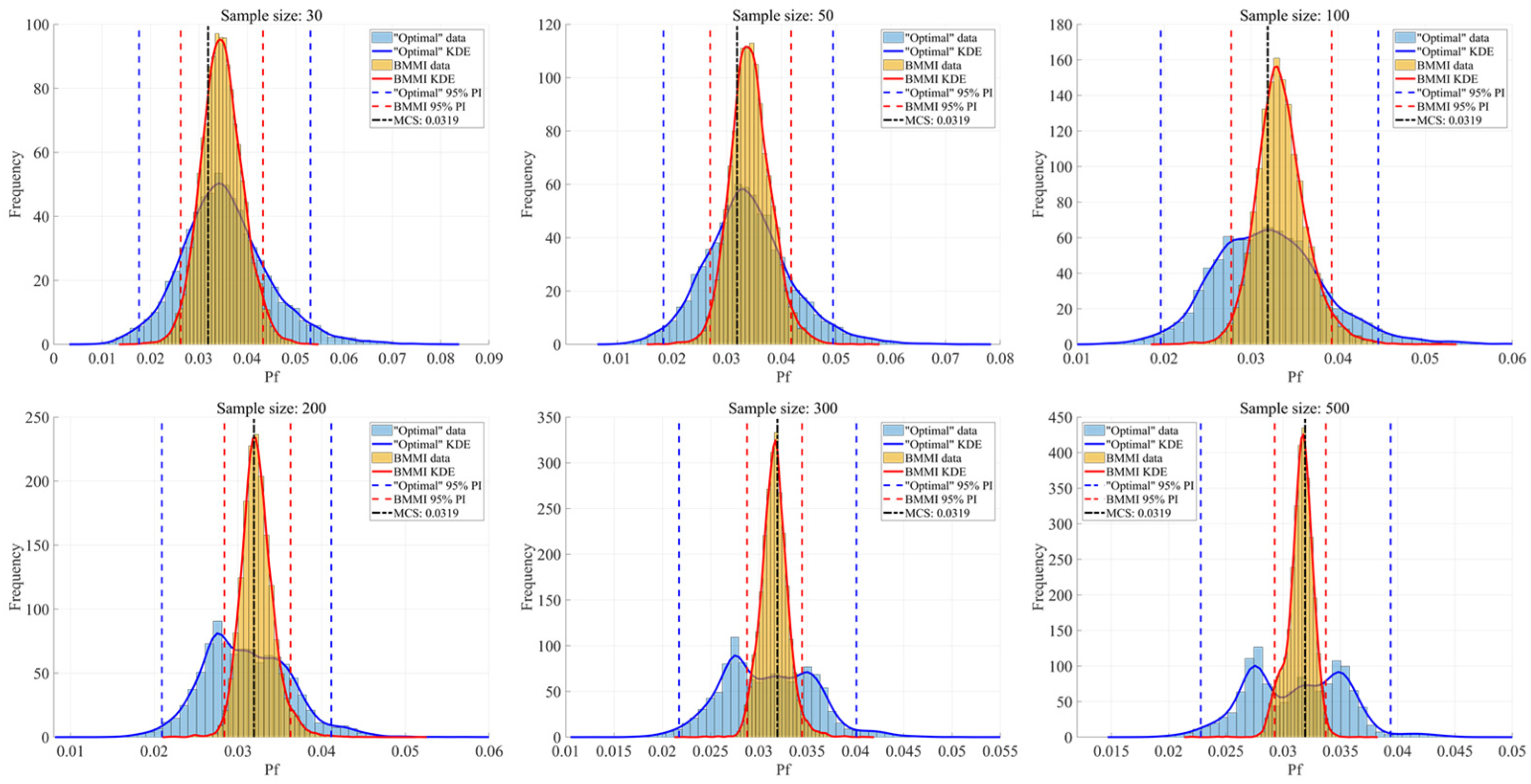
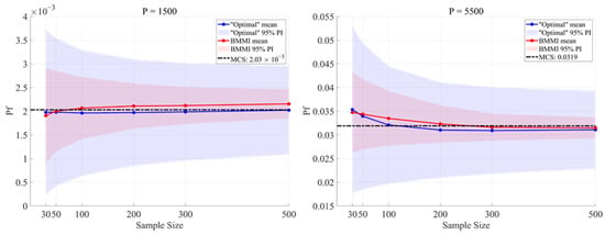
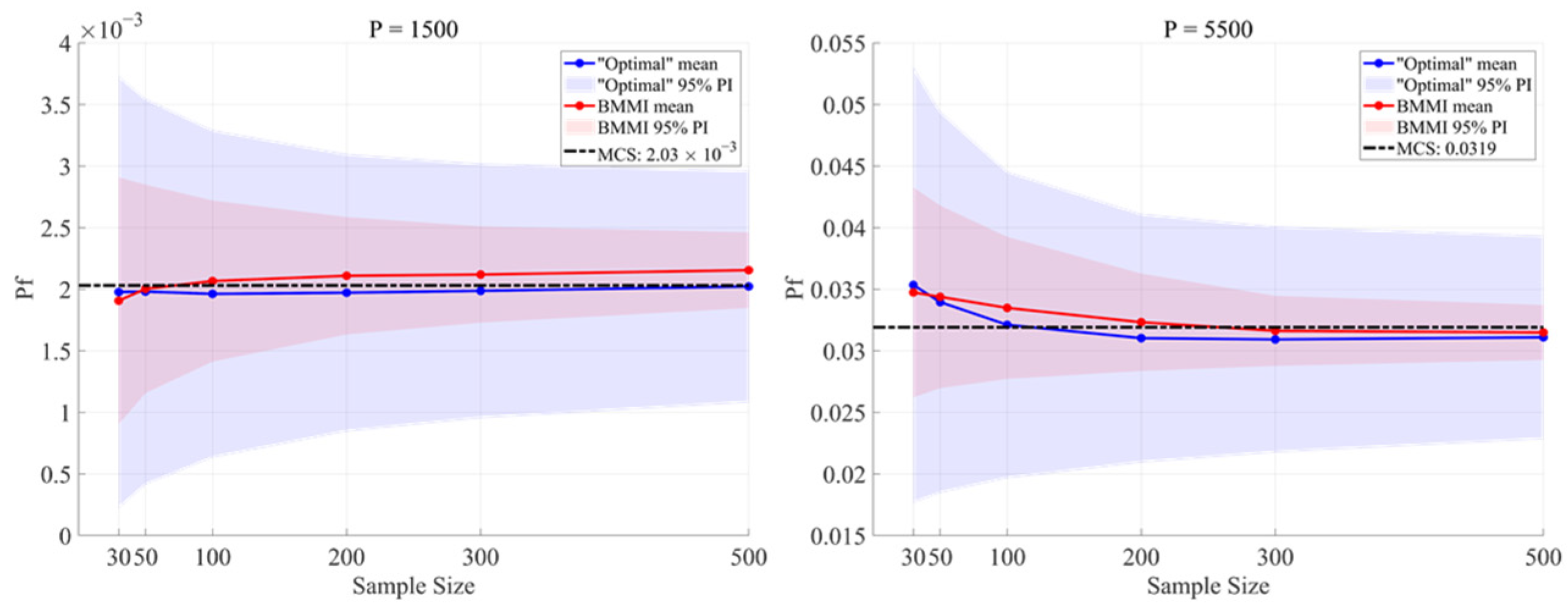
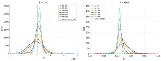
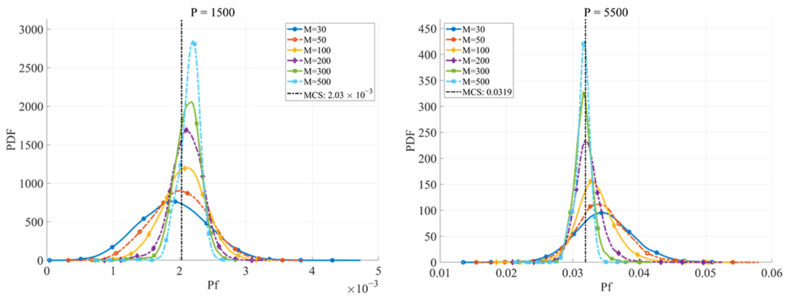
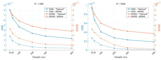
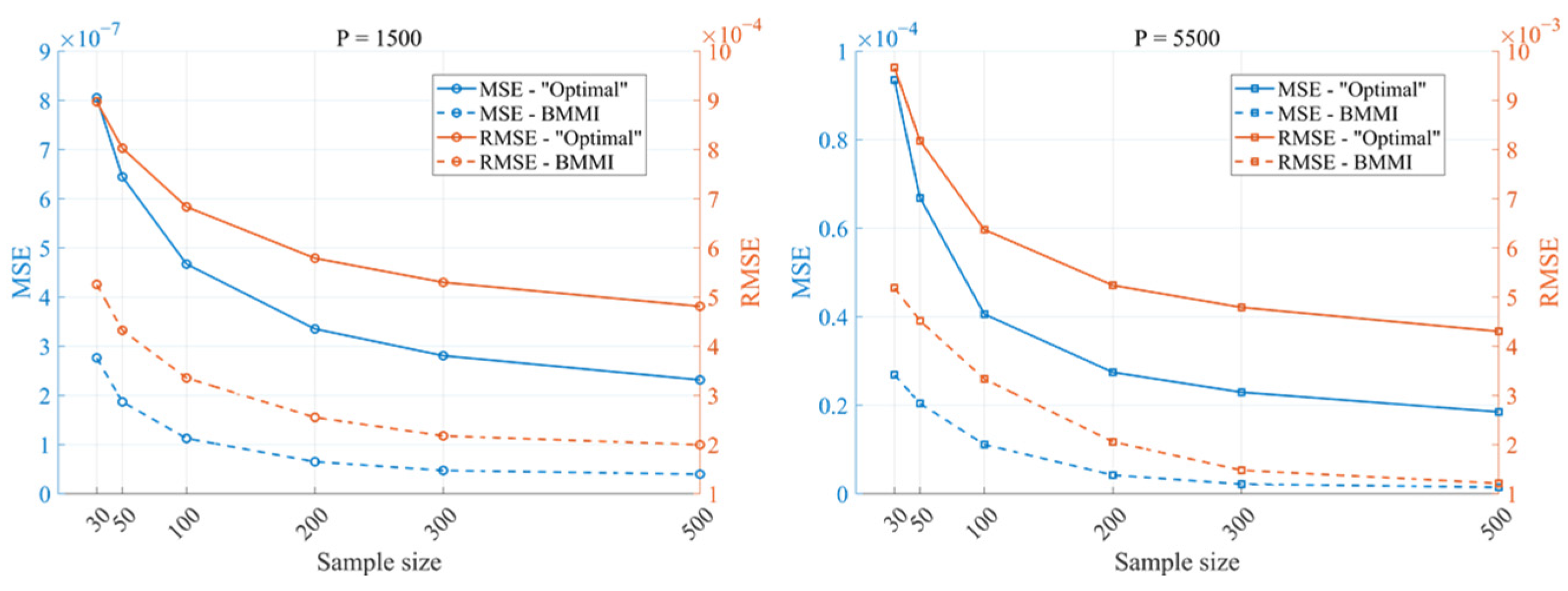

Disclaimer/Publisher’s Note: The statements, opinions and data contained in all publications are solely those of the individual author(s) and contributor(s) and not of MDPI and/or the editor(s). MDPI and/or the editor(s) disclaim responsibility for any injury to people or property resulting from any ideas, methods, instructions or products referred to in the content. |
© 2026 by the authors. Licensee MDPI, Basel, Switzerland. This article is an open access article distributed under the terms and conditions of the Creative Commons Attribution (CC BY) license.