


Abstract
Ocean wave evolution reflects delayed wind forcing, nonlinear wind–wave interactions, and wave persistence, which complicate multi-horizon significant wave height (SWH) forecasting. This study analyzes wind–wave lag relationships and wave memory characteristics in the South China Sea and the Bay of Bengal using ERA5 data from 2022 to 2024, leading to region-specific input windows of 12 h and 21 h. Based on these findings, SSA-STLSTM-LT integrates Wind–Wave Lag Attention, ST-LSTM, a Temporal Transformer, and spatial self-attention within a direct six-horizon forecasting framework. Feature ablation further identifies a nine-variable input configuration. Under a common ERA5-based evaluation protocol, the model achieved horizon-averaged RMSE values of 0.098 m and 0.065 m in Regions A and B, respectively. It obtained the lowest MAE and RMSE across all six horizons in Region A. In Region B, it achieved the lowest RMSE from 3 to 24 h, remained comparable to the best model at 48 h, and was less accurate than the LT-enhanced recurrent baselines at 72 h. Independent altimeter validation further showed favorable observational consistency relative to PredRNN-LT and TrajGRU-LT, with smaller differences in Region B. The results indicate strong but region- and horizon-dependent forecasting advantages.
1. Introduction
Significant wave height (SWH) is one of the most important parameters describing ocean surface conditions and is fundamental to maritime transportation, offshore engineering, marine renewable energy, and coastal hazard mitigation. Accurate SWH forecasting provides critical support for route planning, operational scheduling, and safety assessment, particularly under extreme conditions such as tropical cyclones and storm surges, during which wave fields evolve rapidly and exhibit strong spatiotemporal variability [1,2]. Therefore, developing reliable multi-horizon wave forecasting methods remains an important challenge in ocean prediction.
Operational wave forecasting primarily relies on third-generation spectral wave models, such as WAM, SWAN, and WAVEWATCH III [3,4,5]. These models simulate wave generation, propagation, nonlinear interactions, and dissipation by solving the wave action balance equation and therefore provide physically consistent representations of wave evolution. However, high-resolution regional applications can be computationally demanding and depend strongly on the quality of atmospheric forcing, initial and boundary conditions, and empirical source-term parameterizations [6,7]. With the increasing availability of reanalysis and observational datasets, data-driven deep learning methods have emerged as complementary tools for learning nonlinear relationships between historical environmental conditions and future wave states [8].
Recurrent neural networks and their variants have been widely applied to wave forecasting. LSTM networks can represent long-term temporal dependencies [9,10], while convolutional long short-term memory (ConvLSTM) extends this capability to gridded spatiotemporal fields through convolutional operations [11,12,13]. Trajectory gated recurrent unit (TrajGRU) further improves the representation of non-stationary spatial propagation by learning location-dependent recurrent connections [14,15]. More recently, Transformer-based and hybrid spatiotemporal architectures have been introduced for regional wave forecasting [16,17]. These studies have demonstrated the feasibility of using deep learning to predict the temporal evolution of wave fields. Therefore, the novelty of the present study does not lie simply in applying deep learning to SWH forecasting. Instead, it focuses on the explicit representation of delayed wind–wave interactions and the physically guided selection of region-dependent historical input windows.
Although existing spatiotemporal models can learn spatial correlations and temporal dependencies, the delayed response of wave evolution to wind forcing has not been sufficiently represented. In reality, wave development depends on delayed energy transfer, cumulative wind forcing, swell propagation, and wave persistence. Recent studies on wave source terms and satellite observations have also emphasized the importance of wind input, swell dissipation, and observational validation in wave modeling [18,19]. Moreover, the strength and temporal structure of wind–wave lag relationships can vary among ocean regions because of differences in wave persistence, swell propagation, and environmental conditions. Consequently, applying an identical historical input window to all regions may not adequately represent regional wave dynamics, particularly at longer forecast horizons. Physically informed regional analyses are therefore needed before determining the temporal context used by a forecasting model.
In this study, both the wave-related input variables and the SWH prediction targets are derived from ERA5 reanalysis. The proposed framework should therefore be interpreted as a data-driven model for forecasting the spatiotemporal evolution represented in the ERA5 data domain, rather than as a replacement for operational spectral wave models. Regional wind–wave lag relationships, wave memory characteristics, and cumulative wind forcing effects are first quantitatively analyzed using ERA5 data from the South China Sea and the Bay of Bengal. These analyses provide a physical basis for selecting region-specific historical input windows and guide the subsequent model design.
Based on these findings, a wind–wave lag-aware spatiotemporal forecasting model, termed SSA-STLSTM-LT, is developed. The framework integrates a Wind–Wave Lag Attention mechanism with ST-LSTM, a Temporal Transformer, and spatial self-attention to represent delayed wind forcing, long-range temporal dependencies, and non-local spatial wave field structures. Six horizon-specific Bayesian-regularized prediction heads then generate the 3, 6, 12, 24, 48, and 72 h SWH point forecasts directly from a shared spatiotemporal representation.
The main contributions of this study are summarized as follows.
Wind–wave lag relationships, wave memory characteristics, and cumulative wind forcing effects are systematically quantified in two contrasting ocean regions. The diagnosed regional response characteristics provide a physical basis for selecting region-specific historical input windows.
A Wind–Wave Lag Attention module is developed to explicitly represent the delayed influence of historical wind forcing on wave evolution. This lag-aware representation is integrated with spatiotemporal recurrent learning, spatial self-attention, and long-range temporal modeling in a direct multi-horizon forecasting framework.
The proposed framework is comprehensively evaluated using selected data-driven benchmark models, feature ablation and input window sensitivity experiments, and independent satellite altimeter observations. These experiments assess forecasting accuracy, model component contributions, and observational consistency in the South China Sea and the Bay of Bengal.
2. Materials and Methods
2.1. Study Regions
This study selects two representative ocean regions, the South China Sea (Region A) and the Bay of Bengal (Region B). Figure 1 shows the study area (bathymetry from ETOPO1 is shown as background for geographical reference). Region A (110–130° E, 10–25° N) is mainly affected by seasonal monsoon systems, resulting in relatively regular wind forcing and smoother wave field evolution. Region B (80–100° E, 5–20° N), located in the northern tropical Indian Ocean, is frequently influenced by monsoons, tropical cyclones, and convective systems, leading to stronger non-stationarity and more abrupt SWH variations.
Figure 1.
Locations and spatial domains of Region A in the South China Sea and Region B in the Bay of Bengal.
These two regions represent contrasting wave environments, providing a suitable basis for evaluating the forecasting accuracy and regional generalization capability of the proposed model.
2.2. Datasets
This study utilizes the Fifth-generation European Centre for Medium-Range Weather Forecasts (ECMWF) Reanalysis dataset (ERA5) [20]. ERA5 provides temporally continuous and physically consistent atmospheric and oceanic fields through advanced data assimilation and has been widely applied in ocean wave forecasting studies.
Hourly ERA5 data from 2022 to 2024 were used in this study. The selected variables include significant wave height (SWH), mean wave period (MWP), mean wave direction (MWD), and the 10 m zonal and meridional wind components (U10 and V10). All variables have a temporal resolution of 1 h and a spatial resolution of 0.25° × 0.25°.
2.3. Data Preprocessing
To enhance the representation of wave state evolution and wind–wave interactions, several physically meaningful descriptors were derived from ERA5 variables. MWD was transformed into sine and cosine components (MWD_sin and MWD_cos) to avoid discontinuities at the 0°/360° boundary [21]. Wave energy and wave steepness were further derived to describe wave energy state and wave development characteristics [2,5].
The initial feature set contained 11 variables: SWH, MWP, MWD, MWD_sin, MWD_cos, wave energy, wave steepness, U10, V10, height change rate, and sea state index. Based on feature ablation results, height change rate and sea state index were removed due to limited additional contribution and feature redundancy. The final input configuration therefore included nine variables: SWH, MWP, MWD, MWD_sin, MWD_cos, wave energy, wave steepness, U10, and V10.
All variables were spatially cropped, grid-aligned, and checked for missing values. Wind fields were interpolated onto the wave grid. Each variable was normalized using a robust median–IQR scheme to reduce the influence of outliers, and wave energy was logarithmically transformed before normalization. Sliding temporal windows were then used to construct input–output samples for SWH prediction at lead times of 3, 6, 12, 24, 48, and 72 h.
2.4. Independent Altimeter Observations
Independent Level-3 along-track SWH observations from Copernicus Marine were used for external observational validation. The available altimeter archive covered 2022–2024 within Regions A and B; however, to preserve temporal independence from model development, only observations collocated with forecasts from the temporally held-out test period of 20 July–31 December 2024 were retained for evaluation. Invalid records, missing values, and outliers were removed through quality control. The gridded model predictions and corresponding ERA5 fields were collocated with the altimeter observations using bilinear spatial interpolation and a temporal tolerance of ±1 h. All evaluated models were assessed using the same sets of matched observations at each region and forecast lead time. Negative predicted SWH values were clipped to zero before evaluation. Bias, MAE, RMSE, and PCC were then calculated from the matched pairs to provide an independent observational comparison complementary to the ERA5-based gridded evaluation.
2.5. Physical Characterization of Wind–Wave Lag
Understanding the temporal relationship between wind forcing and wave evolution is essential for physically meaningful wave forecasting. Besides instantaneous wind forcing, wave development is influenced by delayed energy transfer, cumulative wind input, and wave memory effects associated with propagation and swell processes [19,22,23]. To quantify these characteristics and determine appropriate historical input windows, analyses of wind–wave lag correlation, wave memory, cumulative wind forcing, and input-window sensitivity were conducted for both study regions.
2.5.1. Wind–Wave Lag Correlation
Figure 2 illustrates the lag correlation between wind forcing and regional mean SWH. Both regions exhibit clear delayed wind–wave responses, with the highest correlation occurring approximately 7 h after wind forcing under all-sample conditions, indicating that wave evolution is primarily controlled by previous rather than concurrent wind conditions [24].
Figure 2.
Wind–SWH lag correlation in Regions A and B.
For high-wave events, as shown in Table 1, the peak lag remains approximately 7 h in Region A but decreases to approximately 4 h in Region B, suggesting a faster response of extreme waves to recent wind forcing in the Bay of Bengal.
Table 1.
Summary of wind–SWH lag correlation statistics for the two study regions.
2.5.2. Wave Memory Characteristics
Wave evolution also exhibits persistence due to swell propagation and energy storage [25,26]. The autocorrelation function (ACF) of SWH was therefore examined to quantify wave-memory characteristics. As shown in Table 2, SWH autocorrelation indicates strong memory effects in both regions, with consistently longer persistence in Region B. The autocorrelation coefficient decreases below 0.8 after approximately 28 h in Region A and 33 h in Region B, while the corresponding 0.5 threshold occurs after approximately 59 h and 64 h, respectively. These results indicate stronger wave memory characteristics in Region B and suggest that longer historical information is required to adequately represent wave evolution.
Table 2.
Wave memory characteristics derived from the SWH autocorrelation analysis.
2.5.3. Cumulative Wind Forcing
Wave growth depends on cumulative wind energy input rather than instantaneous forcing alone [27]. As shown in Table 3, the cumulative correlation analysis indicates that wind–wave correlation in Region A increases rapidly within the first 12–18 h before approaching saturation, whereas Region B exhibits a more gradual increase over the investigated period. This behavior indicates longer effective forcing timescales and stronger cumulative wind energy effects in Region B.
Table 3.
Correlations between cumulative wind forcing and SWH in the two regions.
2.5.4. Determination of Region-Specific Input Windows
The above analyses indicate that historical input windows should consider not only peak wind–wave lag but also wave memory persistence and cumulative wind forcing. Sensitivity experiments were therefore performed using seven candidate input windows (6, 9, 12, 15, 18, 21, and 24 h), with the results summarized in Table 4 and Table 5. Forecasting performance was evaluated using mean absolute error (MAE), root mean square error (RMSE), and the Pearson correlation coefficient (PCC).
Table 4.
Validation set sensitivity of forecasting performance to the historical input window in Region A.
Table 5.
Validation set sensitivity of forecasting performance to the historical input window in Region B.
Forecasting performance in Region A improved as the input window increased to 12 h, whereas longer windows provided no consistent additional benefit. In Region B, the lowest validation errors were obtained using the 21 h input window, consistent with the region’s longer wave memory and cumulative wind forcing timescales. Accordingly, 12 h was selected for Region A, while 21 h was retained as a physically guided representative setting for Region B.
All physical diagnostics used to guide the input window selection were calculated using the training and validation periods. The seven candidate input windows were compared exclusively on the validation set, and the temporally held-out test set was not accessed during model or input window selection.
To assess sensitivity to random initialization, the selected and neighboring input windows were further evaluated using three random seeds: 42, 2024, and 3407. Specifically, 9, 12, and 15 h were examined for Region A, while 18, 21, and 24 h were examined for Region B. The same training and validation partitions were used across all seeds, and all repeated-window results were calculated on the validation set. Results are reported as mean ± standard deviation. Seed-wise mean RMSE values, averaged across the 3, 6, 12, and 24 h forecast horizons, were further examined using paired t-tests.
2.6. SSA-STLSTM-LT Framework
2.6.1. Overall Architecture
This study proposes a wind–wave lag-aware spatiotemporal model, termed SSA-STLSTM-LT, for direct multi-horizon significant wave height forecasting. The model is designed to capture nonlinear wind–wave interactions, spatial wave field structures, and temporal evolution processes.
As shown in Figure 3, the framework takes multivariate marine environmental fields as input, including wave state descriptors and wind forcing variables. A three-layer spatiotemporal long short-term memory (ST-LSTM) backbone is first employed to extract hierarchical spatiotemporal representations from the observed historical sequence. Spatial self-attention, Wind–Wave Lag Attention, and a Temporal Transformer are subsequently used to enhance non-local spatial dependency modeling, lag-aware wind–wave interaction learning, and long-range temporal representation, respectively.
Figure 3.
Overall architecture of the proposed SSA-STLSTM-LT model. The shared three-layer ST-LSTM, spatial self-attention, lag-aware wind–wave modeling, and Temporal Transformer modules extract a common spatiotemporal representation from the historical nine-channel input sequence. Six horizon-specific Bayesian-regularized prediction heads directly generate the 3, 6, 12, 24, 48, and 72 h SWH point forecasts in parallel without recursive feedback between forecast horizons.
The model adopts a direct multi-horizon forecasting strategy. The historical input sequence is processed by the shared feature extraction backbone to obtain a fused spatiotemporal representation . This representation is distributed in parallel to six horizon-specific Bayesian-regularized prediction heads corresponding to lead times of 3, 6, 12, 24, 48, and 72 h:
where denotes the observed historical input sequence, () represents the shared feature extraction backbone, is the resulting fused spatiotemporal representation, and denotes the Bayesian-regularized prediction head for the -th forecast horizon. All six heads operate directly on the same shared representation. Predictions at shorter lead times are not fed back into the model to generate longer-lead forecasts. Therefore, the proposed model follows a non-recursive direct multi-horizon strategy and avoids autoregressive error propagation across forecast horizons.
2.6.2. ST-LSTM
The spatiotemporal long short-term memory network (ST-LSTM) was originally introduced in PredRNN to model spatiotemporal dependencies through recurrent memory units. Compared with a conventional LSTM, which primarily represents temporal dependencies, ST-LSTM introduces an additional spatial memory state. This dual-memory design enables the model to represent both the temporal evolution and spatial structure of regional wave fields, making it suitable for SWH forecasting.
For clarity, Equations (2)–(12) describe the state update process of a representative ST-LSTM unit. The layer index is omitted to simplify the notation, while the same update mechanism is applied to the stacked ST-LSTM units illustrated in Figure 4.
Figure 4.
Temporal and vertical state propagation within the stacked ST-LSTM backbone. The horizontal recurrence represents the encoding of the observed historical input sequence, while the vertical connections represent information transmission among the stacked ST-LSTM units. The temporal cell state, hidden state, and spatial memory state are propagated through the recurrent backbone to construct hierarchical spatiotemporal representations. The horizontal unfolding does not represent recursive generation of the six future forecast horizons, which are produced directly and in parallel by the horizon-specific prediction heads shown in Figure 3.
Let t denote the current time step. The input field, previous hidden state, and previous temporal cell state are denoted by , , and , respectively. These variables are spatial feature tensors with channel, height, and width dimensions. The notation represents concatenation along the channel dimension.
The temporal cell state is updated using a forget gate, an input gate, and a candidate temporal state:
Here, σ(·) denotes the sigmoid activation function, tanh(·) denotes the hyperbolic tangent function, represents convolution, and ⊙ denotes element-wise multiplication. The variables and represent the forget gate and input gate of the temporal memory branch, respectively. The symbols , , and Wc denote learnable convolution kernels, while , , and denote their corresponding bias terms.
The candidate temporal cell state is represented by , whereas denotes the updated temporal cell state. The forget gate controls the amount of information retained from , while the input gate determines the contribution of the candidate state .
In addition to the temporal cell state, the ST-LSTM unit maintains a spatial memory state. In the following compact unit-level formulation, denotes the incoming spatial memory, while denotes the updated spatial memory. The spatial memory branch is expressed as
Here, the superscript (s) distinguishes the gates and parameters associated with the spatial-memory branch from those associated with the temporal memory branch. The variables and denote the spatial input gate and spatial forget gate, respectively.
The kernels , , and transform the current input field , whereas , , and transform the incoming spatial memory state . Their corresponding bias terms are denoted by , , and .
The candidate spatial memory state is denoted by , and denotes the updated spatial memory state. The spatial input gate controls the incorporation of the candidate state, while the spatial forget gate determines how much information is retained from the incoming spatial memory. In the stacked ST-LSTM backbone, the spatial memory state is propagated through the recurrent units as illustrated schematically in Figure 4.
The updated temporal and spatial memories are then fused to generate the current hidden state. The output gate is calculated as
and the current hidden state is obtained as
Here, denotes the output gate, and represents the concatenation of the updated temporal and spatial memories along the channel dimension. The convolution kernels , , and transform the current input, previous hidden state, and concatenated memory states, respectively, while is the output gate bias.
The kernel and bias transform the fused temporal–spatial memory representation. The resulting hidden state contains information from the current input, the previous hidden representation, the updated temporal cell state, and the updated spatial memory state.
The hidden state is subsequently mapped into a feature representation
where denotes the feature representation derived from the current hidden state. The symbols and denote the learnable kernel and bias of the feature projection operation, respectively, and ϕ(⋅) denotes its nonlinear activation function.
The parameters and are distinguished from and in Equation (2), which are associated specifically with the temporal forget gate. This distinction avoids using the same symbols for different model operations.
The prediction error is quantified using a reconstruction loss jointly calculated over the six directly predicted forecast horizons:
where N denotes the number of training samples and K = 6 denotes the number of forecast horizons. The variables and represent the reference and predicted SWH fields, respectively, for training sample i at forecast horizon k. The field-level MSE is calculated over the corresponding spatial grid points.
The six target horizons correspond to lead times of 3, 6, 12, 24, 48, and 72 h. The reconstruction loss is calculated jointly over the six horizon-specific predictions generated from the same shared spatiotemporal representation.
For the deterministic model variants, is directly used as the training objective. For SSA-STLSTM-LT equipped with Bayesian-regularized prediction heads, constitutes the reconstruction component of the complete variational objective defined in Equation (29).
The horizontal unfolding shown in Figure 4 represents recurrent state propagation during encoding of the observed historical sequence. It does not indicate recursive generation of the six future forecast horizons. Once the historical sequence has been encoded, all six SWH forecasts are generated directly and simultaneously by the parallel horizon-specific Bayesian-regularized prediction heads shown in Figure 3. Predictions at shorter lead times are not fed back into the model to generate forecasts at longer lead times.
2.6.3. Spatial Self-Attention
To capture non-local spatial dependencies, a spatial self-attention (SSA) module is introduced based on the standard attention mechanism [28]. SSA computes correlations among all spatial locations and adaptively aggregates information across the wave field. The calculation is expressed as Equation (14):
where , , and denote the query, key, and value matrices, respectively, and denotes the dimension of the key vectors. This module enables the network to represent large-scale spatial interactions, high-wave regions, and gradient transition zones that are difficult to capture using local convolution alone.
2.6.4. Lag-Aware Temporal Modeling
Wind–Wave Lag Representation
The analysis in Section 2.5 shows that wave evolution responds to wind forcing with a measurable time lag. To represent this delayed response, a Wind–Wave Lag Attention module is designed to adaptively learn the contribution of historical wind forcing to the current wave state.
Assuming that the current time step is , the wave state feature at this time is represented as , and the corresponding historical wind field feature sequence is defined as
where denotes the wind field feature at time and denotes the maximum lag time step.
To adaptively model the contributions of wind fields at different lag time steps, this study adopts a Query–Key mechanism. Specifically, the current wave state feature is used as the Query, while the historical wind field sequence is used as both the Key and the Value. The corresponding linear mapping forms can be expressed as Equations (15) and (16):
where and denote the learnable mapping matrices for Query, Key and Value, respectively.
Subsequently, the correlation score is calculated according to the similarity between the Query and the Key of each lagged wind field feature, as shown in Equation (17):
where denotes the dimension of the Key vector.
The correlation scores are further normalized using the Softmax function [29], as expressed in Equation (18):
where represents the relative contribution of the wind field at time to the current wave state .
The lag-aware wind representation is obtained by weighted aggregation, as shown in Equation (19):
where denotes the lag-aware wind representation.
Finally, the lag-aware wind field representation is fused with the current wave state feature to obtain the joint wind–wave feature, as expressed in Equation (20):
where denotes the fused wind–wave feature, and represents the feature concatenation operation. This representation is then fed into the subsequent network modules to further model the coupled evolution process of wind and waves.
This design explicitly incorporates delayed wind forcing information into the spatiotemporal representation, thereby enabling the network to model lagged wind–wave interactions. The overall architecture of the Wind–Wave Lag Attention module is illustrated in Figure 5.
Figure 5.
Structure of the Wind–Wave Lag Attention module. Wave state features are used as queries, while the historical wind feature sequence provides the keys and values. The resulting cross-attention weights represent the temporal correspondence between the evolving wave state and preceding wind forcing, and the attention-weighted wind context is subsequently combined with the wave representation. In the implementation, the wave and wind feature sequences are spatially pooled into temporal tokens before cross-attention, and the final lag-aware token is used as the wind–wave lag context in the subsequent multi-source fusion.
Temporal Transformer
The Temporal Transformer is introduced to model long-range temporal dependencies in wave evolution [28]. Unlike recurrent networks, it enables parallel computation and global dependency modeling through self-attention.
Given an input feature sequence
A learnable positional embedding is added:
The temporal self-attention operation is defined as
Furthermore, a multi-head attention is calculated as
where the projections are parameter matrices: .
The model uses the feed-forward neural network to further perform nonlinear feature transformation, as expressed in Equation (25):
where GELU denotes the Gaussian Error Linear Unit activation function [30]. Through global temporal attention, the Temporal Transformer captures persistent wind forcing, wave energy accumulation, and long-term propagation effects.
The output of the Temporal Transformer is denoted by Ztemp, which summarizes the long-range temporal dependencies contained in the top-layer ST-LSTM hidden-state sequence. In parallel, the Wind–Wave Lag Attention module produces a lag-aware wind–wave representation Zlag, while denotes the final hidden feature map generated by the top ST-LSTM layer at the last observed time step.
Before fusion, Ztemp and Zlag are expanded over the spatial dimensions to match . The three representations are then concatenated and processed by a multi-source fusion block. Spatial self-attention and a subsequent feature projection operation are applied to obtain the final fused spatiotemporal representation Zt:
Here, [·] denotes channel-wise concatenation, and denote learnable convolutional mappings, and ϕ(·) denotes the nonlinear feature transformation. The final representation , rather than the isolated output of the Temporal Transformer, is supplied to the six horizon-specific Bayesian-regularized prediction heads.
2.6.5. Bayesian-Regularized Multi-Horizon Prediction Head
To regularize the horizon-specific predictors and reduce overfitting, a lightweight Bayesian-regularized multi-horizon prediction head is introduced after the shared feature extraction backbone [31]. The final fused spatiotemporal representation Zt, obtained after multi-source fusion, spatial self-attention, and feature projection, is distributed in parallel to six horizon-specific Bayesian-regularized prediction heads. Each head has its own prediction parameters and is responsible for one predefined forecast horizon.
For the h-th forecast horizon, the prediction obtained under the m-th stochastic weight sample is expressed as
where denotes the SWH prediction for the h-th forecast horizon under the m-th stochastic evaluation, and denotes the corresponding random weight sample. Each head directly maps the shared representation to its designated forecast horizon, and no output from one head is used as the input to another head.
The Bayesian-regularized model is trained using
where is the joint six-horizon reconstruction loss defined in Equation (13), W represents the collection of random weights in the prediction heads, (w) denotes their variational posterior distribution, and denotes the corresponding prior distribution. The KL divergence term constrains the variational posterior and acts as a regularizer for the horizon-specific prediction parameters. The coefficient controls the contribution of the KL divergence term. A KL warm-up strategy is adopted, in which is gradually increased during the early training epochs to improve optimization stability.
During inference, the Bayesian prediction heads are evaluated M times using independently sampled weights. The final point forecast is obtained by Monte Carlo model averaging:
In this study, M = 20 stochastic evaluations are used to reduce the sampling variability of the final point prediction. Within each evaluation, all six forecast horizons are generated directly from the same shared representation. Therefore, the repeated stochastic evaluations constitute model averaging rather than recursive multi-step forecasting. The forecasting performance is evaluated using Bias, MAE, RMSE, and PCC. The architecture and inference procedure of the six Bayesian-regularized horizon-specific prediction heads are illustrated in Figure 6.
Figure 6.
Architecture of the Bayesian-regularized direct multi-horizon prediction heads. The fused spatiotemporal representation Zt is provided in parallel to six horizon-specific heads corresponding to lead times of 3, 6, 12, 24, 48, and 72 h. Within each head, the input representation undergoes a horizon-specific feature transformation followed by stochastic sampling of the Bayesian output-layer weights. During inference, M = 20 stochastic forward evaluations are performed for each horizon, and the resulting mean predictions are averaged to obtain the reported deterministic SWH point forecast. The six forecast horizons are generated independently without recursive feedback between heads. Each prediction head internally produces mean and scale outputs; however, only the Monte Carlo-averaged mean is used for the deterministic evaluation reported in this study, and the scale output is not interpreted as calibrated predictive uncertainty.
2.7. Experimental Settings
All experiments were implemented in Python 3.10 using the PyTorch framework and trained on an NVIDIA GeForce RTX 3060 Ti GPU with 8 GB of memory.
The ERA5 reanalysis dataset described in Section 2.2 was used for model training and evaluation. Based on the physical analyses presented in Section 2.5, region-specific historical input windows of 12 h for Region A and 21 h for Region B were adopted. The final input configuration consisted of nine variables, and SWH forecasts were generated at lead times of 3, 6, 12, 24, 48, and 72 h.
2.7.1. Temporal Data Partitioning
To avoid information leakage caused by the strong temporal autocorrelation of SWH and the overlap between adjacent sliding windows, the raw hourly records were divided chronologically before sample generation. The training, validation, and temporally held-out test periods were 1 January 2022–6 February 2024, 7 February–19 July 2024, and 20 July–31 December 2024, respectively. Sliding windows were constructed independently within each period, and no input or forecast target was allowed to cross the subset boundaries. With input lengths of 12 h for Region A and 21 h for Region B, the training, validation, and test sets contained 18,325, 3853, and 3877 samples for Region A, and 18,316, 3844, and 3868 samples for Region B, respectively. No random sample-level splitting was applied, and all normalization parameters were estimated exclusively from the training period and subsequently applied unchanged to the validation and test sets.
2.7.2. Benchmark and Reference Models
The proposed SSA-STLSTM-LT model was compared with Linear, ConvLSTM, TrajGRU, PredRNN, TrajGRU-LT, PredRNN-LT, Informer, and FEDformer. A persistence forecast was additionally introduced as a non-trainable reference baseline to assess whether the evaluated models provided predictive value beyond the strong temporal persistence of SWH.
In this study, Linear was implemented as a pixel-wise autoregressive linear model. For each spatial grid point , the historical sequence containing T time steps and C = 9 input variables was flattened into a TC-dimensional feature vector A shared affine transformation was then applied to generate the one-step-ahead SWH prediction:
where w and b are trainable parameters shared across all spatial grid points. Thus, the Linear model captures linear temporal relationships between the historical predictors and SWH but does not explicitly model spatial interactions between neighboring grid points. Multi-step forecasts were generated recursively. After each prediction, the predicted SWH replaced the SWH channel in the latest input frame, whereas the remaining predictor variables retained their latest available values. The historical window was then shifted forward by one step, and the same linear mapping was repeatedly applied until the required forecast horizon was reached.
For a forecast initialized at time t, the persistence prediction at lead time h was defined as
where is the latest observed SWH at grid point (i,j). The same initial SWH field was used for all forecast lead times. Persistence and all trainable models were evaluated using the same temporally held-out test samples, ocean masks, valid grid points, and inverse normalization procedure.
The forecast generation strategy followed the design of each model. Linear, ConvLSTM, TrajGRU, PredRNN, TrajGRU-LT, and PredRNN-LT generated continuous hourly forecasts recursively, and their outputs at 3, 6, 12, 24, 48, and 72 h were extracted for evaluation. The recurrent baselines followed the same feedback rule as Linear: the predicted SWH was fed back into the SWH channel, while the remaining predictor channels retained their latest available values. Informer and FEDformer directly generated the continuous future sequence in a single forward pass, from which the six target horizons were selected. SSA-STLSTM-LT directly generated the six predefined forecast horizons from the shared representation without recursive feedback. The persistence baseline directly assigned the latest observed SWH field to each target horizon.
2.7.3. Training and Implementation Details
To improve reproducibility, a fixed random seed of 42 was used for Python, NumPy 1.26.4, PyTorch 2.0.0, and CUDA 11.8, and deterministic cuDNN 8.7.0 execution was enabled. For the main multi-model comparison, each trainable model was evaluated using one controlled training run with the common random seed of 42. This protocol was adopted to maintain consistent randomization control across the evaluated architectures. However, a common fixed seed does not quantify run-to-run variability. Therefore, the differences reported in the main benchmark tables are interpreted as numerical comparisons under the controlled fixed-seed setting rather than as statistically significant cross-seed differences. The repeated-seed experiments in the present study were limited to the input window robustness analysis. All trainable models were optimized using Adam with an initial learning rate of 1 × 10⁻⁴ and a maximum training budget of 80 epochs. The benchmark models were trained for the full 80 epochs without early termination, whereas SSA-STLSTM-LT employed validation-based early stopping with a patience of 15 epochs. In all cases, checkpoint selection relied exclusively on the validation set, and the temporally held-out test set was used only for final evaluation without further parameter adjustment. The main architectural and training configurations of SSA-STLSTM-LT are summarized in Table 6.
Table 6.
Main architectural and training configurations of SSA-STLSTM-LT.
To ensure consistent comparisons, all models used the same chronological data partitions, nine predictor variables, region-specific input lengths, forecast lead times, ocean masks, inverse normalization procedure, and evaluation metrics. For the Linear and deterministic recurrent models, including ConvLSTM, TrajGRU, PredRNN, TrajGRU-LT, and PredRNN-LT, the checkpoint with the lowest aggregate validation MSE across the six target horizons was retained. For Informer and FEDformer, the checkpoint with the lowest validation loss was selected. For SSA-STLSTM-LT, training was terminated when the validation variational loss did not decrease for 15 consecutive epochs, and the checkpoint with the lowest validation variational loss was retained for final evaluation.
The principal architectural configurations, forecast generation strategies, batch sizes, and computational costs of the evaluated models are summarized in Table 7.
Table 7.
Principal architectural configurations, forecast strategies, and computational costs of the evaluated models.
2.7.4. Evaluation Metrics
Model performance was evaluated using bias, mean absolute error (MAE), root mean squared error (RMSE), and the Pearson correlation coefficient (PCC). Let and denote the observed and predicted SWH values, respectively, and let N denote the total number of valid prediction–observation pairs over all test samples and valid ocean grid points. The metrics were calculated as
Positive bias indicates systematic overestimation, whereas negative bias indicates underestimation. MAE and RMSE are expressed in metres, while PCC is dimensionless. All metrics were computed after transforming the normalized predictions and observations back to the physical SWH scale and were evaluated only over valid ocean grid points.
Because SWH exhibits strong temporal persistence, high PCC and low absolute errors alone may not establish whether a model provides predictive value beyond persistence. Therefore, an RMSE-based skill score was introduced:
A positive indicates that the evaluated model outperforms persistence, whereas = 0 indicates equivalent performance. A negative value indicates inferior performance relative to persistence. For example, = 0.20 corresponds to a 20% reduction in RMSE. The skill score was calculated separately for each region and forecast lead time.
3. Results
3.1. Overall Comparison
Table 8 and Table 9 summarize the overall forecasting performance of the evaluated models in Regions A and B, respectively. Prediction errors generally increase with forecast lead time, reflecting the decreasing predictability of wave evolution at longer forecast horizons. However, the relative performance of the models varies between the two study regions.
Table 8.
Overall performance comparison of the evaluated models in Region A.
Table 9.
Overall performance comparison of the evaluated models in Region B.
In Region A, SSA-STLSTM-LT achieves the lowest MAE and RMSE values across all six forecast horizons and maintains the highest or jointly highest PCC values. Its relative advantage becomes more evident at medium and extended lead times. TrajGRU-LT and PredRNN-LT remain the strongest recurrent comparison models, but their errors increase more rapidly than those of SSA-STLSTM-LT as the forecast horizon extends.
In Region B, SSA-STLSTM-LT achieves the lowest RMSE values over the 3–24 h horizons. At 48 h, its RMSE is comparable to that of PredRNN-LT at the reported precision, while its MAE remains slightly lower. At 72 h, PredRNN-LT and TrajGRU-LT achieve lower RMSE and MAE values, whereas SSA-STLSTM-LT remains competitive.
The recurrent models generally outperform the Linear and Transformer-based baselines at medium and extended lead times, highlighting the value of explicitly representing spatiotemporal wave evolution. Informer remains competitive at short lead times, particularly in Region B, whereas the errors of Informer and FEDformer increase more rapidly at longer lead times.
Overall, SSA-STLSTM-LT achieves the lowest horizon-averaged RMSE in both study regions. Nevertheless, the results do not indicate universal superiority at every region–lead time combination, because the LT-enhanced recurrent baselines remain more accurate at the 72 h horizon in Region B. The relative model advantages should therefore be interpreted as region- and horizon-dependent.
Because the main benchmark comparison was conducted using one controlled run for each model, small numerical differences should be interpreted cautiously. In particular, SSA-STLSTM-LT and PredRNN-LT have the same reported RMSE of 0.091 m at 48 h in Region B, indicating comparable performance at the reported precision. At 72 h, the ordering among SSA-STLSTM-LT, PredRNN-LT, and TrajGRU-LT should likewise not be interpreted as a statistically significant cross-seed ranking. Although the Region A differences are generally larger, no cross-seed significance claim is made for the main model comparison.
3.2. Forecast Skill Relative to Persistence
Because SWH is strongly autocorrelated, the persistence forecast retains high PCC values, particularly at short lead times. This indicates that a high correlation coefficient alone is insufficient to establish forecast skill beyond persistence. The RMSE-based skill scores relative to persistence are summarized in Table 10.
Table 10.
RMSE-based forecast skill scores relative to persistence in Regions A and B.
SSA-STLSTM-LT achieves positive RMSE skill scores in both regions and at all forecast lead times. Based on the recalculated values, its skill scores range from approximately 0.54 to 0.81 in Region A and from approximately 0.48 to 0.77 in Region B. These values indicate substantial RMSE reductions relative to persistence, particularly at medium and extended lead times.
The positive skill scores demonstrate that the forecasting performance of SSA-STLSTM-LT cannot be explained solely by the intrinsic temporal persistence of SWH. Nevertheless, the relative ranking among learning-based models varies by region and forecast horizon. The negative skill score of Linear at the 3 h horizon in Region B also illustrates that persistence remains a competitive reference for strongly autocorrelated short-range forecasts.
3.3. Spatial Forecasting Performance
3.3.1. Spatial Error Distribution
Figure 7, Figure 8, Figure 9 and Figure 10 present the spatial distributions of Bias and RMSE for different models in the two study regions. Overall, prediction errors increase with forecast lead time, although the spatial growth patterns vary substantially among models.
Figure 7.
Full-test-set spatial distribution of mean Bias in Region A. Bias is calculated at each valid ocean grid point over all temporally held-out test samples.
Figure 8.
Full-test-set spatial distribution of mean Bias in Region B. Bias is calculated at each valid ocean grid point over all temporally held-out test samples.
Figure 9.
Full-test-set spatial distribution of mean RMSE in Region A. RMSE is calculated at each valid ocean grid point over all temporally held-out test samples.
Figure 10.
Full-test-set spatial distribution of mean RMSE in Region B. RMSE is calculated at each valid ocean grid point over all temporally held-out test samples.
In Region A, the largest errors are concentrated near coastlines, island-dense areas, and regions with strong SWH gradients. Compared with the evaluated benchmark models, SSA-STLSTM-LT generally maintains lower RMSE values and comparatively homogeneous spatial error patterns across the selected forecast horizons.
In Region B, several benchmark models develop broader regions of systematic bias and elevated RMSE as lead time increases. SSA-STLSTM-LT preserves relatively extensive low-error areas at short and medium lead times, although the differences among the strongest models narrow at the longest horizon.
These spatial patterns are consistent with the aggregate metrics reported in Table 8 and Table 9. They indicate that SSA-STLSTM-LT can preserve large-scale wave field structures while limiting spatial error growth. However, the maps should be interpreted as spatial diagnostic evidence rather than as direct proof of physical realism.
3.3.2. Case Studies
Figure 11 and Figure 12 present representative forecasting cases from the two study regions at multiple forecast lead times. Compared with statistical metrics, individual cases provide a more intuitive assessment of each model’s ability to reconstruct wave field structures, recover high-wave regions, and represent propagation processes.
Figure 11.
Spatial comparison for representative test sample 1732 in Region A. The panels show the ERA5 reference SWH fields and the corresponding model predictions at the forecast horizons indicated in the figure.
Figure 12.
Spatial comparison for representative test sample 599 in Region B. The panels show the ERA5 reference SWH fields and the corresponding model predictions at the forecast horizons indicated in the figure.
In Region A, which is characterized by complex coastlines, numerous islands, and highly heterogeneous wave conditions, the differences among models are particularly evident. SSA-STLSTM-LT successfully preserves the location, extent, and propagation direction of major wave height bands throughout the forecasting horizon. In contrast, the benchmark models exhibit varying degrees of displacement, amplitude distortion, or structural fragmentation, especially at longer lead times.
In Region B, SSA-STLSTM-LT also maintains high consistency with the reference wave fields, accurately reproducing dominant spatial gradients and the overall distribution of high-wave regions. Although some benchmark models can capture the large-scale wave field structure, they tend to produce excessive smoothing, local noise, or propagation path deviations as the forecast lead time increases.
In the selected cases, SSA-STLSTM-LT preserves the dominant wave height gradients and major high-wave areas more consistently than most benchmark models, particularly at medium and extended lead times. Because these figures represent individual test samples, they are interpreted as complementary qualitative evidence and not as a substitute for the full-sample statistical comparison.
3.4. Seasonal Forecasting Performance
Figure 13 and Figure 14 show the seasonal Taylor diagram evaluation results for the two study regions at the 24 h forecast lead time. Seasonal variability influences model performance to some extent; however, the overall ranking of the models remains largely unchanged across seasons.
Figure 13.
Seasonal Taylor diagram comparison of the evaluated models in Region A at the 24 h lead time. The angular coordinate denotes PCC, the radial distance denotes the standard deviation, and the distance from the ERA5 reference point represents the centered RMSE.
Figure 14.
Seasonal Taylor diagram comparison of the evaluated models in Region B at the 24 h lead time. The angular coordinate denotes PCC, the radial distance denotes the standard deviation, and the distance from the ERA5 reference point represents the centered RMSE.
Region A exhibits more pronounced seasonal performance variations, with larger model dispersion during winter than during spring and summer. In Region B, the model points are more concentrated, indicating smaller seasonal differences under the ERA5-based evaluation.
In most seasonal panels, SSA-STLSTM-LT lies close to the ERA5 reference point and shows a favorable balance among PCC, centered RMSE, and standard deviation. The relative positions of the LT-enhanced recurrent models vary among seasons, indicating that the benefit of lag-aware temporal modeling is not identical under all seasonal conditions.
Overall, SSA-STLSTM-LT maintains competitive and generally stable seasonal performance in both regions. These results support its adaptability across different seasonal wave regimes without implying uniform superiority in every seasonal subset.
3.5. Ablation Study
3.5.1. Model Component Ablation
Table 11 presents the configurations corresponding to the ablation experiments. Table 12 and Table 13 summarize the ablation study results for different model configurations. Although forecasting errors increase with lead time for all configurations, the relative performance differences clearly reveal the contributions of individual model components.
Table 11.
Component ablation configurations of SSA-STLSTM-LT.
Table 12.
Ablation study results in Region A.
Table 13.
Ablation study results in Region B.
The Temporal Transformer improves the performance of configuration I by introducing long-range temporal dependency modeling. However, the magnitude of the improvement varies with region and forecast horizon, indicating that temporal self-attention alone does not fully represent the delayed coupling between wind forcing and wave evolution.
The Bayesian-regularized prediction heads further reduce the deterministic point forecast errors. This improvement is consistent with a regularization and Monte Carlo model-averaging effect, which may reduce overfitting and sampling variability in the horizon-specific predictors. Because predictive uncertainty calibration was not evaluated, these improvements should not be interpreted as evidence of calibrated probabilistic uncertainty.
Adding Wind–Wave Lag Attention to the Bayesian configuration produces modest and region-dependent improvements when configurations III and IV are compared. The complete configuration V achieves the best overall ablation performance, indicating complementarity among lag-aware wind–wave modeling, temporal Transformer encoding, spatial self-attention, and Bayesian regularization rather than a uniformly dominant isolated contribution from a single component.
The complete SSA-STLSTM-LT configuration achieves the best overall performance among the evaluated ablation variants in both regions. This result indicates complementarity among spatial self-attention, long-range temporal modeling, lag-aware wind–wave representation, and Bayesian regularization with Monte Carlo model averaging. Collectively, these components provide a more comprehensive representation of historical wave states, wind forcing, delayed responses, and future wave evolution.
3.5.2. Input-Feature Ablation
To evaluate the contributions of different input variables to significant wave height forecasting, an input feature ablation study was conducted using eight feature configurations (F0–F7) derived from the complete SSA-STLSTM-LT framework. Specific feature groups were progressively added or removed to investigate their relative importance for wave forecasting.
Table 14 and Table 15 summarize the ablation results for Regions A and B, respectively. Overall, forecasting performance depends not only on the number of input variables but also on the physical relevance of the information they provide. Compared with configurations using only the original wave and wind variables, the inclusion of directional encodings and wave physics features consistently improves forecasting performance, indicating that these variables provide complementary dynamical information for representing wind–wave interactions.
Table 14.
Input feature ablation results in Region A.
Table 15.
Input feature ablation results in Region B.
The directional encodings (MWD_sin and MWD_cos) effectively eliminate the discontinuity associated with circular directional data and enhance the representation of wave propagation characteristics. Meanwhile, Wave energy and Wave steepness provide additional information regarding wave energy states and wave development conditions, thereby improving the description of complex wave field evolution.
In contrast, Height change rate and Sea state index contribute relatively little to forecasting skill. In both study regions, removing these variables does not degrade performance and instead yields the best overall results. This finding suggests that the information contained in these variables is already represented by other wave-related features and therefore introduces limited additional predictive value.
Notably, both regions exhibit highly consistent feature contribution patterns. Configuration F7 achieves the best overall performance in Regions A and B, demonstrating that retaining directional encodings and wave physics variables while excluding the dynamic sea state indicators provides a more effective feature combination.
Based on these results, a final nine-variable configuration consisting of SWH, MWP, MWD, MWD_sin, MWD_cos, Wave energy, Wave steepness, U10, and V10 was adopted in all subsequent experiments. This configuration reduces input redundancy while improving forecasting accuracy and model interpretability.
Overall, the feature ablation results indicate that physically meaningful directional and wave state descriptors substantially enhance the representation of wind–wave coupling processes, whereas the contribution of empirical dynamic sea state indicators remains limited. These findings highlight the importance of physically informed feature selection for regional significant wave height forecasting.
3.5.3. Input Window Robustness Validation
To further examine whether the selected input windows were robust to random initialization and stochastic model training, repeated experiments were conducted using three random seeds (42, 2024, and 3407). For each region, the selected input window and its neighboring windows were evaluated. Specifically, 9, 12, and 15 h were tested for Region A, while 18, 21, and 24 h were tested for Region B. The same data partitions were used across random seeds to isolate the influence of model training randomness. For each seed, the evaluation metrics were first averaged over the 3, 6, 12, and 24 h forecast horizons, and the final results are reported as mean ± standard deviation in Table 16.
Table 16.
Repeated-seed validation of the selected and neighboring input windows using three random seeds.
As shown in Table 16, the repeated validation results in Region A are consistent with the original input window sensitivity analysis. The 12 h input window achieved the lowest mean MAE and RMSE, with values of 0.049 ± 0.0007 m and 0.073 ± 0.0007 m, respectively. Compared with the 9 h and 15 h windows, the 12 h window reduced the mean RMSE by approximately 0.003 m and 0.010 m, respectively. The relatively small standard deviation also indicates that the performance of the 12 h window was stable across different random seeds. These results support the robustness of selecting 12 h as the representative historical input window for Region A.
For Region B, the repeated validation results show that the 18, 21, and 24 h windows produced comparable performance, although the 21 h window achieved the lowest mean RMSE and the highest mean PCC. The mean RMSE values were 0.048 ± 0.0007 m, 0.048 ± 0.0011 m, and 0.052 ± 0.0029 m for the 18, 21, and 24 h windows, respectively. The difference between the 18 h and 21 h windows was very small, indicating that Region B is relatively insensitive to input window variations within the 18–21 h range. The 24 h window showed slightly larger errors and greater variability, suggesting that excessively long historical inputs may introduce redundant or noisy information.
Paired t-tests based on seed-wise mean RMSE were further conducted to assess the statistical robustness of the selected input windows. In Region A, the 12 h window showed a statistically supported advantage over the neighboring windows, significantly outperforming both the 9 h window (p = 0.031) and the 15 h window (p = 0.017). These results provide statistical support for the robustness of the 12 h input window across the three evaluated random seeds. In Region B, although the 21 h window achieved the lowest average error, its advantage over the neighboring windows was not statistically significant. The p-values were 0.782 for 21 h versus 18 h, 0.165 for 21 h versus 24 h, and 0.290 for 24 h versus 18 h. Therefore, the Region B result should not be interpreted as a sharply defined statistical optimum. Instead, it indicates a broad effective input window range of approximately 18–24 h, within which the 21 h window was retained as a physically guided representative setting because it is consistent with the stronger wave memory and cumulative wind forcing characteristics identified in Region B.
Overall, the repeated-seed validation supports the robustness of the 12 h input window in Region A, whereas Region B exhibits a wider effective historical input range. In Region B, the 21 h window should therefore be regarded as a physically guided representative setting rather than a statistically dominant optimum. This additional analysis quantifies the influence of training randomness and provides a more reliable basis for the region-specific input window selection.
3.6. Extreme Event Forecasting
3.6.1. Extreme Sea States
To evaluate forecasting performance under severe wave conditions, the top 10% of test samples ranked by spatially averaged significant wave height were selected as extreme sea state cases. The performance of SSA-STLSTM-LT was compared with that of TrajGRU-LT and PredRNN-LT across multiple forecast lead times.
Figure 15 and Figure 16 show that RMSE generally increases and PCC decreases with forecast lead time under the selected extreme-sea-state subset, indicating increasing forecast difficulty at longer horizons. SSA-STLSTM-LT achieves lower RMSE and generally higher PCC than the two LT-based recurrent comparison models at most evaluated horizons. The differences are more pronounced in Region B, whereas the three models become more similar at the 72 h horizon in Region A.
Figure 15.
Lead-time variation in (a) RMSE and (b) PCC under extreme sea conditions in Region A.
Figure 16.
Lead-time variation in (a) RMSE and (b) PCC under extreme sea conditions in Region B.
Regional comparisons show that the RMSE values under the selected extreme conditions are generally higher in Region B than in Region A. Nevertheless, SSA-STLSTM-LT exhibits a smaller increase in error than the two comparison models in Region B, indicating favorable relative robustness under the evaluated severe wave conditions.
The density scatter distributions shown in Figure 17 and Figure 18 further illustrate the behavior of SSA-STLSTM-LT under extreme conditions. Strong linear consistency between predictions and reference values is observed at all forecast lead times, with most samples concentrated near the 1:1 reference line. Although scatter dispersion gradually increases at longer lead times and slight underestimation appears in the highest wave range, the model continues to capture the overall variability of extreme wave heights effectively.
Figure 17.
Density scatter comparison between SSA-STLSTM-LT predictions and ERA5 reference SWH values under extreme sea conditions at different forecast lead times in Region A. The dashed line denotes the 1:1 reference line, and the color scale represents point density.
Figure 18.
Density scatter comparison between SSA-STLSTM-LT predictions and ERA5 reference SWH values under extreme sea conditions at different forecast lead times in Region B. The dashed line denotes the 1:1 reference line, and the color scale represents point density.
Overall, SSA-STLSTM-LT exhibits strong fitting capability and forecasting stability under extreme sea states. These results suggest that lag-aware wind–wave representation and long-term temporal dependency modeling contribute substantially to the prediction of extreme wave events.
3.6.2. Typhoon Events
To further examine the generalization capability of the proposed framework under unseen extreme weather conditions, two representative tropical cyclone events within the temporally held-out test period were selected: Typhoon Trami over the South China Sea in October 2024 and Cyclone Dana over the Bay of Bengal in October 2024. The two events occurred in different marine environments and exhibited distinct wave field characteristics, thereby providing complementary case studies under extreme sea states.
Figure 19 and Figure 20 present representative 24 h forecasts for the two events. In the selected snapshots, SSA-STLSTM-LT reproduces the principal location, spatial extent, and intensity pattern of the high-wave regions. Compared with the reference fields, the benchmark models exhibit larger localized deviations in wave intensity and peak wave position, particularly near the centers of the high-wave areas.
Figure 19.
Spatial distribution characteristics at a representative moment during Typhoon Trami (06:00 on 30 October 2024, 24 h forecast lead time).
Figure 20.
Spatial distribution characteristics at a representative moment during Tropical Cyclone Dana (12:00 on 23 October 2024, 24 h forecast lead time).
The corresponding error distributions show that the errors of SSA-STLSTM-LT are mainly concentrated near local boundaries of the high-wave regions, whereas PredRNN-LT and TrajGRU-LT exhibit broader deviations within some of the energetic wave areas. These case-specific results suggest that SSA-STLSTM-LT retains the spatial structure of the extreme wave fields more effectively under the two evaluated events.
Figure 21 and Figure 22 illustrate the temporal evolution of the SSA-STLSTM-LT forecasts during the two events. As the tropical cyclones evolved, the predicted high-wave regions changed continuously in location, extent, and intensity. The model generally reproduced the corresponding evolution of the reference wave fields, although localized differences remained around the high-gradient regions.
Figure 21.
Spatio-temporal evolution characteristics of SSA-STLSTM-LT during Typhoon Trami (00:00, 06:00, and 12:00 on 30 October 2024, 24 h forecast lead time).
Figure 22.
Spatio-temporal evolution characteristics of SSA-STLSTM-LT during Cyclone Dana (12:00 on 23 October, 06:00 and 18:00 on 24 October 2024, 24 h forecast lead time).
Overall, the two held-out case studies provide additional evidence that SSA-STLSTM-LT can reproduce the principal spatial and temporal characteristics of extreme wave fields under different regional conditions. Its advantages over the comparison models are more evident in some high-wave and high-gradient areas. Nevertheless, these results are based on two representative events and should be interpreted as complementary case evidence rather than a comprehensive assessment of all tropical cyclone conditions.
3.7. Independent Validation
To assess the observational generalization of the evaluated models, Level-3 along-track significant wave height observations from Copernicus Marine were used as an independent validation dataset. Unlike the gridded evaluation based on ERA5, the altimeter measurements were not involved in model training, validation, or checkpoint selection.
The predictions of SSA-STLSTM-LT, PredRNN-LT, and TrajGRU-LT, together with the corresponding ERA5 fields, were collocated with the same altimeter observations using identical temporal and spatial interpolation procedures. PredRNN-LT and TrajGRU-LT were selected because they were the strongest learning-based comparison models in the gridded evaluation and provide the most direct architectural comparisons with the proposed method. For each region and lead time, all models were evaluated using the same set of matched satellite observations.
Table 17 presents the resulting Bias, MAE, RMSE, and PCC values. In Region A, SSA-STLSTM-LT achieves the lowest RMSE and the highest PCC among the three forecasting models at all evaluated lead times. The differences become more evident at medium and extended lead times, where PredRNN-LT and TrajGRU-LT exhibit stronger error growth. In Region B, the differences among the models are smaller; nevertheless, SSA-STLSTM-LT retains the lowest RMSE at every lead time and achieves the highest or jointly highest PCC.
Table 17.
Independent validation of ERA5 and the three forecasting models against satellite altimeter observations.
The ERA5–altimeter error remains comparatively stable across lead times in both regions. This behavior indicates that the absolute model–altimeter discrepancy contains a background component associated with differences between ERA5 and satellite observations, in addition to errors introduced by forecasting and spatiotemporal collocation. Therefore, the altimeter validation metrics should not be interpreted as pure model forecast errors.
Figure 23 shows the lead time evolution of RMSE and PCC. The ERA5 curves remain nearly unchanged, whereas the forecasting models generally exhibit increasing RMSE and decreasing PCC as the forecast horizon extends. Relative to PredRNN-LT and TrajGRU-LT, SSA-STLSTM-LT remains closer to the ERA5 reference curve over most lead times, with the clearest separation occurring in Region A. These results indicate that SSA-STLSTM-LT exhibits the smallest increase in error relative to the ERA5 reference among the three evaluated forecasting models.
Figure 23.
Lead-time variation in (a) RMSE in Region A; (b) PCC in Region A; (c) RMSE in Region B; and (d) PCC in Region B, evaluated against the matched satellite altimeter observations.
Figure 24 presents the density scatter distributions at the representative 24 h lead time. SSA-STLSTM-LT shows a more concentrated distribution around the 1:1 reference line, particularly in Region A, whereas the two comparison models exhibit greater dispersion. TrajGRU-LT performs slightly better than PredRNN-LT in Region A, while PredRNN-LT shows a modest advantage in Region B, consistent with the region-dependent behavior reported in Table 17.
Figure 24.
Density scatter comparison against satellite altimeter observations at the 24 h lead time.
All three forecasting models show increasing deviations under higher wave conditions. A similar tendency is also present in the ERA5–altimeter comparison, suggesting that part of the model–observation discrepancy is associated with the reanalysis target itself. The additional dispersion of the model predictions reflects the combined effects of model forecast error, satellite sampling and representativeness differences, and spatiotemporal collocation uncertainty.
Overall, the independent validation provides comparative observational evidence that SSA-STLSTM-LT generalizes more favorably than PredRNN-LT and TrajGRU-LT under the evaluated conditions. However, the differences are region-dependent and are smaller in Region B. Moreover, because the models were trained using ERA5 as the target, their absolute agreement with satellite observations remains partly constrained by the discrepancy between ERA5 and the altimeter measurements. The satellite analysis is therefore interpreted as an independent comparative generalization assessment rather than as a direct measurement of forecast error alone.
4. Discussion
SSA-STLSTM-LT provided positive forecast skill beyond persistence in both regions, while its performance relative to the learning-based benchmarks varied between the two regional wave regimes.
4.1. Interpretation of the Lag-Aware Representation
The forecasting improvements can be attributed in part to the explicit representation of delayed wind–wave interactions. Rather than assuming that historical wind forcing and wave responses contribute synchronously, the Wind–Wave Lag Attention module adaptively assigns different contributions to wind features at different preceding time steps. The ablation results indicate that incorporating this lag-aware representation improves the description of the temporal relationship between wind forcing and wave evolution. In combination with the Temporal Transformer and spatial self-attention, the framework represents delayed forcing, long-range temporal dependencies, and non-local spatial correlations within a unified spatiotemporal architecture. This representation is particularly relevant to longer forecast horizons, for which cumulative forcing and wave persistence become increasingly important.
4.2. Regional Dependence of Historical Input Windows
The selected historical input windows differ between the two regions, consistent with their distinct wave evolution characteristics. Region A exhibits a shorter wave memory timescale and a more rapid saturation of cumulative wind forcing, for which a 12 h historical window provides sufficient temporal context. In contrast, Region B exhibits stronger wave persistence and a greater influence of swell propagation, supporting the use of a longer 21 h input window. These findings suggest that the historical input length should be selected according to regional wind–wave response characteristics rather than applying an identical temporal setting to all regions.
4.3. Practical Implications and Limitations
Once trained, the proposed framework enables rapid inference and may serve as a data-driven complement for regional multi-horizon SWH forecasting. Its relatively low inference cost may be useful for applications requiring timely regional wave field estimates, including marine navigation, offshore operations, and coastal risk assessment. However, the input wave variables and prediction targets used in this study are derived from ERA5 reanalysis. Consequently, the model learns and extrapolates the spatiotemporal evolution represented in the ERA5 data domain and does not independently simulate wave generation, propagation, and dissipation processes.
The proposed model was not compared with operational forecasts produced by WAM, SWAN, or WAVEWATCH III under matched atmospheric forcing, initialization, and boundary conditions. Therefore, the present results demonstrate performance relative to the selected data-driven benchmarks rather than superiority over operational spectral wave models. In addition, the network does not explicitly impose physical conservation constraints. Although the satellite–altimeter comparison provides an independent assessment of observational consistency, broader validation against buoy observations, additional satellite datasets, and operational wave forecasts is still required. Future work will investigate physics-informed constraints, forecast atmospheric forcing, and evaluation under operational forecasting conditions.
A further limitation is that the complete multi-model benchmark was conducted using a common fixed random seed rather than repeated independently across multiple seeds. The repeated-seed analysis in the present study focused on the input window robustness experiment. Consequently, Table 8 and Table 9 provide controlled numerical comparisons but do not quantify the run-to-run uncertainty of the complete model ranking. Future work should repeat the strongest architectures across additional random seeds and report cross-seed variability and statistical comparisons for the complete benchmark.
5. Conclusions
This study developed a wind–wave lag-aware deep learning framework, SSA-STLSTM-LT, for multi-horizon significant wave height forecasting in the South China Sea and the Bay of Bengal. Analyses of wind–wave lag relationships, wave memory characteristics, and cumulative wind forcing revealed distinct regional response timescales. Based on these analyses, historical input windows of 12 h and 21 h were selected for the two regions, respectively.
Guided by the diagnosed regional characteristics, the proposed framework integrates ST-LSTM, Wind–Wave Lag Attention, a Temporal Transformer, and spatial self-attention to represent delayed wind forcing, long-range temporal dependencies, and non-local spatial wave field structures. Six Bayesian-regularized horizon-specific prediction heads directly generate SWH point forecasts at lead times of 3, 6, 12, 24, 48, and 72 h from a shared spatiotemporal representation. The feature ablation experiments further identified an effective nine-variable input configuration.
Under the common fixed-seed ERA5-based evaluation protocol, SSA-STLSTM-LT demonstrated positive forecast skill relative to persistence in both study regions and achieved the lowest horizon-averaged RMSE among the evaluated models. In Region A, it obtained the lowest MAE and RMSE values across all six forecast horizons. In Region B, it achieved the lowest RMSE values over the 3–24 h horizons, remained comparable to the best-performing model at 48 h, and was outperformed by the LT-enhanced recurrent baselines at 72 h. Independent altimeter validation further indicated more favorable observational consistency for SSA-STLSTM-LT than for PredRNN-LT and TrajGRU-LT under the matched evaluation conditions, although the differences were smaller in Region B.
These findings support the applicability of the framework across the two evaluated regional settings while showing that its relative performance remains dependent on forecast horizon and regional wave conditions. Because the main benchmark comparison was based on one controlled training run per model using the common random seed of 42, the reported rankings should be interpreted as numerical comparisons under the fixed-seed setting rather than as statistically significant cross-seed conclusions. The framework should be regarded as a data-driven complement for forecasting ERA5-represented regional wave evolution rather than as a replacement for operational spectral wave models. Future work should extend the complete benchmark to repeated independent training runs and evaluate the framework using broader observational datasets and operational forecasting conditions.
Author Contributions
Software, writing—original draft, formal analysis, X.Z.; supervision, project administration, methodology, Y.C.; data curation, resources, writing, Y.L. and D.X.; funding acquisition, J.S. All authors have read and agreed to the published version of the manuscript.
Funding
Science and Technology Plan of Liaoning Province (2024JH2/102400061); Dalian Science and Technology Innovation Fund (2024JJ11PT007, 2025JJ12GX014); Dalian Science and Technology Program for Innovation Talents of Dalian (2022RJ06); Liaoning Province Education Department Scientific research platform construction project (LJ232410158056); and Basic scientific research funds of Dalian Ocean University (2024JBPTZ001), Liaoning Province Data Center Project (2025JH27/10100005); Liaoning Provincial Science and Technology Plan Joint Program (Natural Science Foundation—Doctoral Research Startup Project), Grant No. 2025-BSLH-079.
Institutional Review Board Statement
Not applicable.
Informed Consent Statement
Not applicable.
Data Availability Statement
The ERA5 reanalysis data and Copernicus Marine satellite observations used in this study are publicly available from their respective data providers. The source code, core model implementations, region-specific configuration files, preprocessing procedures, chronological data partition routines, and scripts for the main ERA5-based training and evaluation experiments are publicly available at https://github.com/puffktening/ssa-stlstm-lt-reproducibility (accessed on 21 July 2026). The manuscript-aligned code state is preserved as the versioned GitHub release v1.0.1. The complete processed gridded datasets and full model output archives are not currently deposited in a public repository. However, the released preprocessing procedures, variable definitions, normalization settings, temporal split definitions, and model configurations support reconstruction of the experimental inputs from the publicly available source datasets.
Acknowledgments
We thank the Data Support from National Marine Scientific Data Center (Dalian) (http://odc.dlou.edu.cn/), National Science & Technology Infrastructure, Liaoning Marine and Polar Science Data Center, Dalian Marine Science Data Center for providing valuable data and information. We also thank the reviewers for carefully reviewing the manuscript and providing valuable comments to help improve this paper.
Conflicts of Interest
The authors declare no conflicts of interest.
Abbreviations
The following abbreviations are used in this manuscript:
| ERA5 | Fifth-generation ECMWF atmospheric reanalysis |
| ECMWF | European Centre for Medium-Range Weather Forecasts |
| SWH | Significant wave height |
| MWD | Mean wave direction |
| MWP | Mean wave period |
| U10 | 10 m zonal wind component |
| V10 | 10 m meridional wind component |
| ST-LSTM | Spatiotemporal long short-term memory |
| SSA | Spatial self-attention |
| LT | Lag-aware temporal module |
| KL | Kullback–Leibler divergence |
| RMSE | Root mean square error |
| MAE | Mean absolute error |
| PCC | Pearson correlation coefficient |
| FFN | Feed-forward network |
| ACF | Autocorrelation function |
| ConvLSTM | Convolutional long short-term memory |
| TrajGRU | Trajectory gated recurrent unit |
| PredRNN | Predictive recurrent neural network |
References
- Young, I.R. Wind Generated Ocean Waves, 1st ed.; Elsevier Ocean Engineering Book Series; Elsevier: Amsterdam, The Netherlands; New York, NY, USA, 1999; ISBN 978-0-08-043317-2. [Google Scholar]
- Holthuijsen, L.H. Waves in Oceanic and Coastal Waters; Cambridge University Press: Cambridge, UK, 2007. [Google Scholar]
- Group, T.W. The WAM Model—A Third Generation Ocean Wave Prediction Model. J. Phys. Oceanogr. 1988, 18, 1775–1810. [Google Scholar] [CrossRef] [Scilit]
- Booij, N.; Ris, R.C.; Holthuijsen, L.H. A Third-generation Wave Model for Coastal Regions: 1. Model Description and Validation. J. Geophys. Res. 1999, 104, 7649–7666. [Google Scholar] [CrossRef] [Scilit]
- Tolman, H.L. User Manual and System Documentation of WAVEWATCH III Version 3.14; NOAA/NWS/NCEP/MMAB: Camp Springs, MD, USA, 2009; p. 194. [Google Scholar]
- Janssen, P. The Interaction of Ocean Waves and Wind, 1st ed.; Cambridge University Press: Cambridge, UK, 2004; ISBN 978-0-521-46540-3. [Google Scholar]
- Cavaleri, L.; Alves, J.-H.G.M.; Ardhuin, F.; Babanin, A.; Banner, M.; Belibassakis, K.; Benoit, M.; Donelan, M.; Groeneweg, J.; Herbers, T.H.C.; et al. Wave Modelling—The State of the Art. Prog. Oceanogr. 2007, 75, 603–674. [Google Scholar] [CrossRef] [Scilit]
- LeCun, Y.; Bengio, Y.; Hinton, G. Deep Learning. Nature 2015, 521, 436–444. [Google Scholar] [CrossRef] [Scilit] [PubMed]
- Hochreiter, S.; Schmidhuber, J. Long Short-Term Memory. Neural Comput. 1997, 9, 1735–1780. [Google Scholar] [CrossRef] [Scilit] [PubMed]
- Minuzzi, F.C.; Farina, L. A Deep Learning Approach to Predict Significant Wave Height Using Long Short-Term Memory. Ocean Model. 2023, 181, 102151. [Google Scholar] [CrossRef] [Scilit]
- Shi, X.; Chen, Z.; Wang, H.; Yeung, D.-Y.; Wong, W.; Woo, W. Convolutional LSTM Network: A Machine Learning Approach for Precipitation Nowcasting. In Advances in Neural Information Processing Systems 28; Curran Associates, Inc.: Red Hook, NY, USA, 2015; Volume 28, pp. 802–810. [Google Scholar]
- Gao, Z.; Liu, X.; Yv, F.; Wang, J.; Xing, C. Learning Wave Fields Evolution in North West Pacific with Deep Neural Networks. Appl. Ocean. Res. 2023, 130, 103393. [Google Scholar] [CrossRef] [Scilit]
- Song, T.; Han, R.; Meng, F.; Wang, J.; Wei, W.; Peng, S. A Significant Wave Height Prediction Method Based on Deep Learning Combining the Correlation between Wind and Wind Waves. Front. Mar. Sci. 2022, 9, 983007. [Google Scholar] [CrossRef] [Scilit]
- Shi, X.; Gao, Z.; Lausen, L.; Wang, H.; Yeung, D.-Y.; Wong, W.; Woo, W. Deep Learning for Precipitation Nowcasting: A Benchmark and A New Model. In Advances in Neural Information Processing Systems 30; Curran Associates, Inc.: Red Hook, NY, USA, 2017; Volume 30, pp. 5617–5627. [Google Scholar]
- Yu, M.; Wang, Z.; Song, D.; Zhu, Z.; Pan, R. Spatio-Temporal Ocean Wave Conditions Forecasting Using MA-TrajGRU Model in the South China Sea. Ocean Eng. 2024, 291, 116486. [Google Scholar] [CrossRef] [Scilit]
- Liu, Y.; Lu, W.; Wang, D.; Lai, Z.; Ying, C.; Li, X.; Han, Y.; Wang, Z.; Dong, C. Spatiotemporal Wave Forecast with Transformer-Based Network: A Case Study for the Northwestern Pacific Ocean. Ocean Model. 2024, 188, 102323. [Google Scholar] [CrossRef] [Scilit]
- Liu, Y.; Li, D.; Gong, X.; Feng, J.; Liu, H.; Qi, J.; Yin, B. A Coupled Swin Transformer-LSTM Network for High-Resolution Ocean Wave Forecasting: A Reanalysis-Driven Skill Assessment in the Chinese Marginal Seas. J. Sea Res. 2026, 210, 102670. [Google Scholar] [CrossRef] [Scilit]
- Liu, Q.; Rogers, W.E.; Babanin, A.V.; Young, I.R.; Romero, L.; Zieger, S.; Qiao, F.; Guan, C. Observation-Based Source Terms in the Third-Generation Wave Model WAVEWATCH III: Updates and Verification. J. Phys. Oceanogr. 2019, 49, 489–517. [Google Scholar] [CrossRef] [Scilit]
- Ardhuin, F.; Stopa, J.E.; Chapron, B.; Collard, F.; Husson, R.; Jensen, R.E.; Johannessen, J.; Mouche, A.; Passaro, M.; Quartly, G.D.; et al. Observing Sea States. Front. Mar. Sci. 2019, 6, 124. [Google Scholar] [CrossRef] [Scilit]
- Hersbach, H.; Bell, B.; Berrisford, P.; Hirahara, S.; Horányi, A.; Muñoz-Sabater, J.; Nicolas, J.; Peubey, C.; Radu, R.; Schepers, D.; et al. The ERA5 Global Reanalysis. Q. J. R. Meteorol. Soc. 2020, 146, 1999–2049. [Google Scholar] [CrossRef] [Scilit]
- Wilks, D.S. Statistical Methods in the Atmospheric Sciences, 3rd ed.; International Geophysics Series; Elsevier: Amsterdam, The Netherlands; Academic Press: Boston, MA, USA, 2011; ISBN 978-0-12-385022-5. [Google Scholar]
- Stopa, J.E.; Ardhuin, F.; Girard-Ardhuin, F. Wave Climate in the Arctic 1992–2014: Seasonality and Trends. Cryosphere 2016, 10, 1605–1629. [Google Scholar] [CrossRef] [Scilit]
- Quilfen, Y.; Chapron, B. Ocean Surface Wave-Current Signatures from Satellite Altimeter Measurements. Geophys. Res. Lett. 2019, 46, 253–261. [Google Scholar] [CrossRef] [Scilit]
- Deike, L. Mass Transfer at the Ocean–Atmosphere Interface: The Role of Wave Breaking, Droplets, and Bubbles. Annu. Rev. Fluid Mech. 2022, 54, 191–224. [Google Scholar] [CrossRef] [Scilit]
- Zaug, C.R.; Carter, J.D. Dissipative Models of Swell Propagation across the Pacific. Stud. Appl. Math. 2021, 147, 1519–1537. [Google Scholar] [CrossRef] [Scilit]
- Zheng, C.; Wu, D.; Wu, H.; Guo, J.; Shen, C.; Tian, C.; Tian, X.; Xiao, Z.; Zhou, W.; Li, C. Propagation and Attenuation of Swell Energy in the Pacific Ocean. Renew. Energy 2022, 188, 750–764. [Google Scholar] [CrossRef] [Scilit]
- Xu, Y.; Yu, X. Enhanced Formulation of Wind Energy Input into Waves in Developing Sea. Prog. Oceanogr. 2020, 186, 102376. [Google Scholar] [CrossRef] [Scilit]
- Vaswani, A.; Shazeer, N.; Parmar, N.; Uszkoreit, J.; Jones, L.; Gomez, A.N.; Kaiser, Ł.; Polosukhin, I. Attention Is All You Need. In Advances in Neural Information Processing Systems 30; Curran Associates, Inc.: Red Hook, NY, USA, 2017; Volume 30, pp. 5998–6008. [Google Scholar]
- Bahdanau, D.; Cho, K.; Bengio, Y. Neural Machine Translation by Jointly Learning to Align and Translate. In Proceedings of the 3rd International Conference on Learning Representations, San Diego, CA, USA, 7–9 May 2015. [Google Scholar]
- Hendrycks, D.; Gimpel, K. Gaussian Error Linear Units (GELUs). arXiv 2016, arXiv:1606.08415. [Google Scholar]
- Blundell, C.; Cornebise, J.; Kavukcuoglu, K.; Wierstra, D. Weight Uncertainty in Neural Networks. In Proceedings of the 32nd International Conference on Machine Learning, Lille, France, 6–11 July 2015; PMLR: Lille, France, 2015; Volume 37, pp. 1613–1622. [Google Scholar]
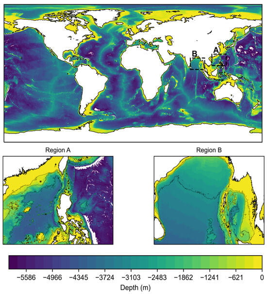
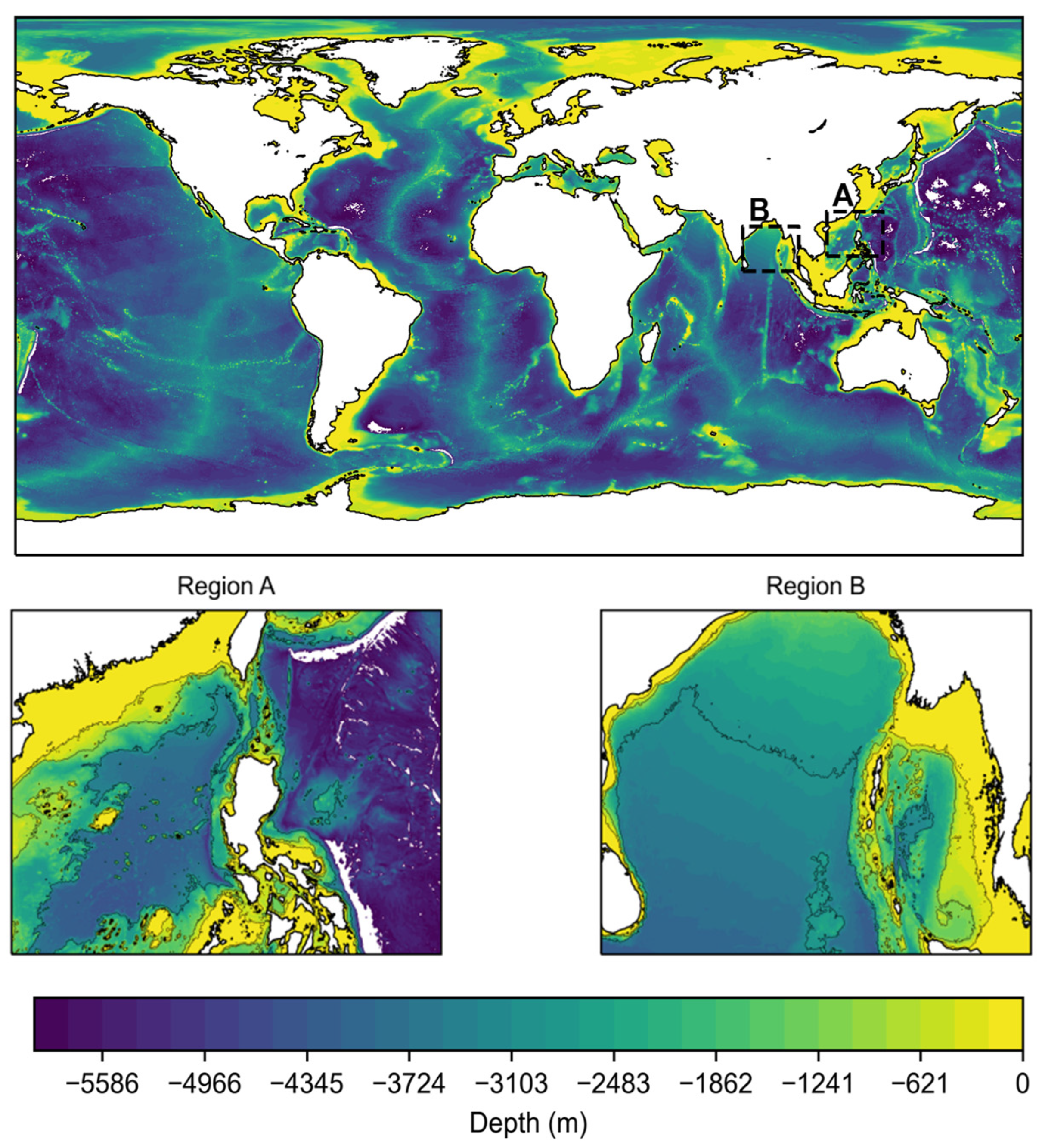
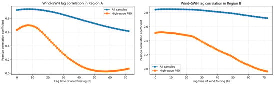
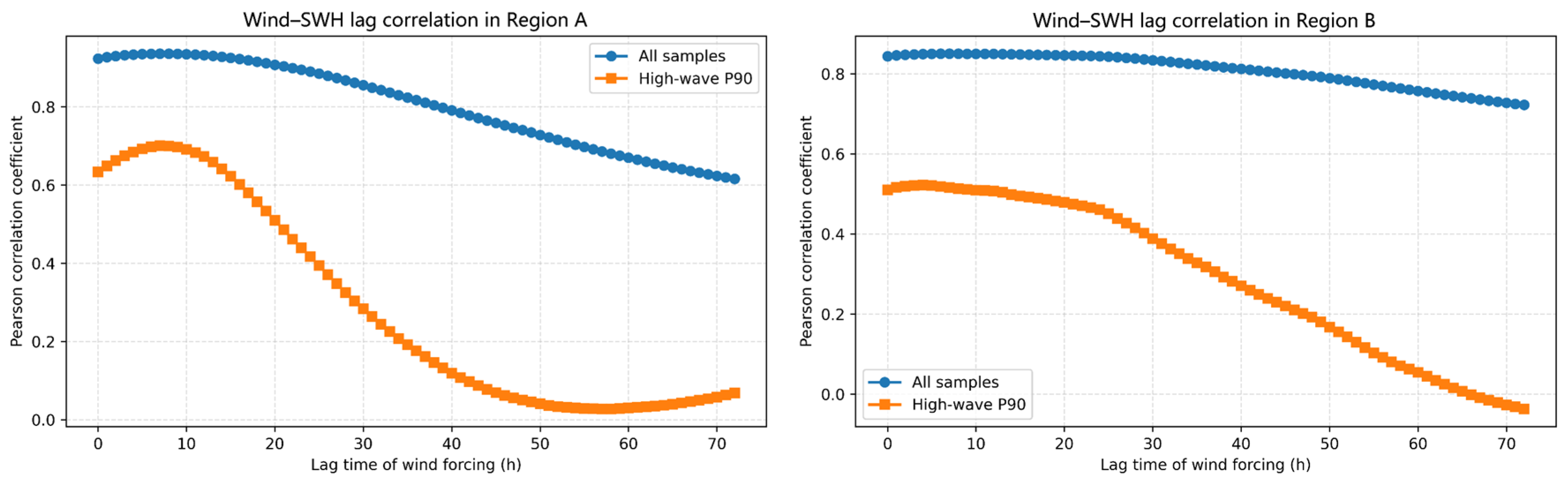
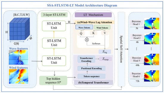
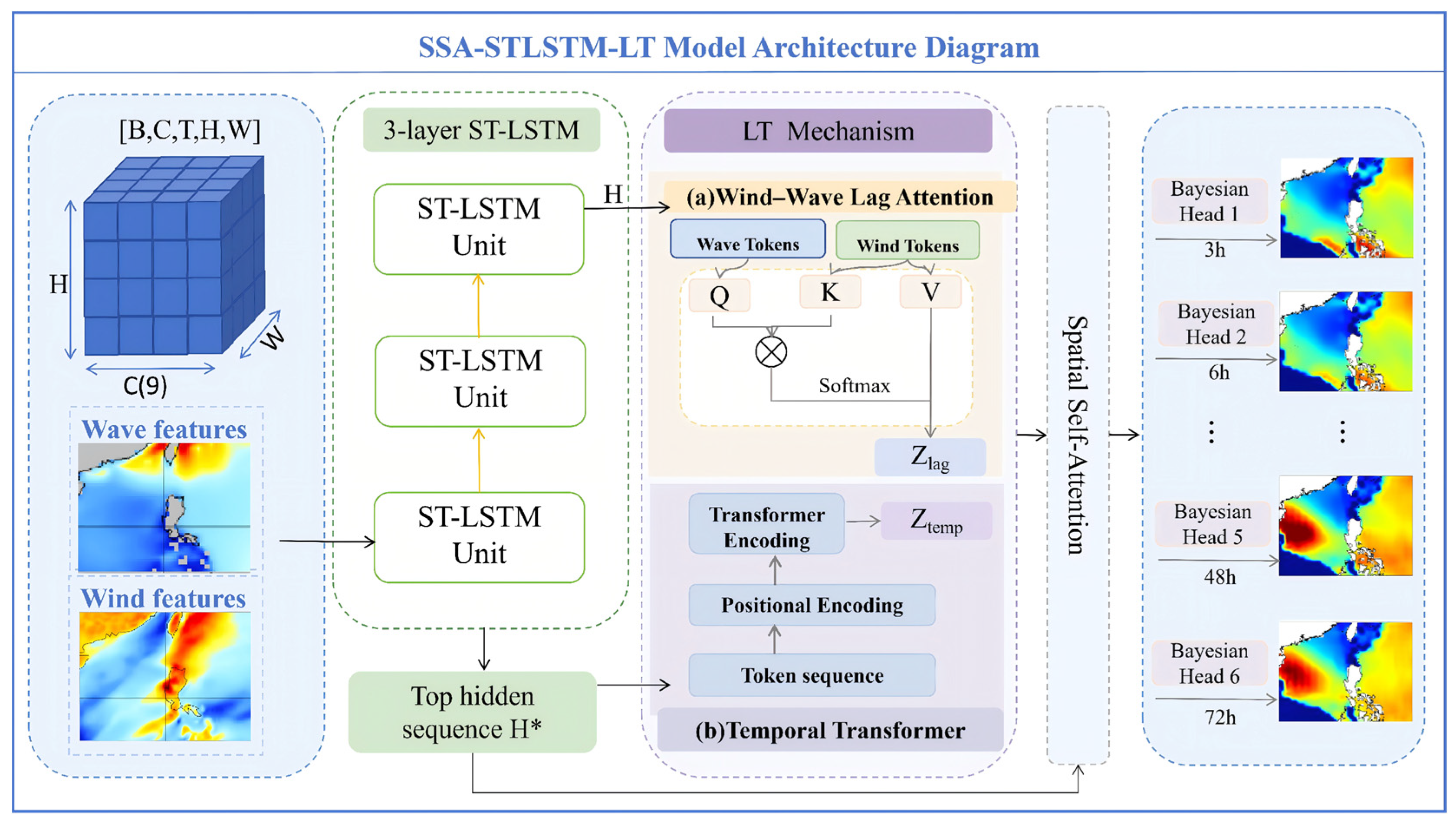
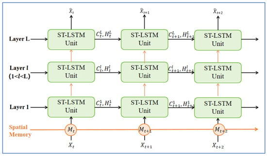
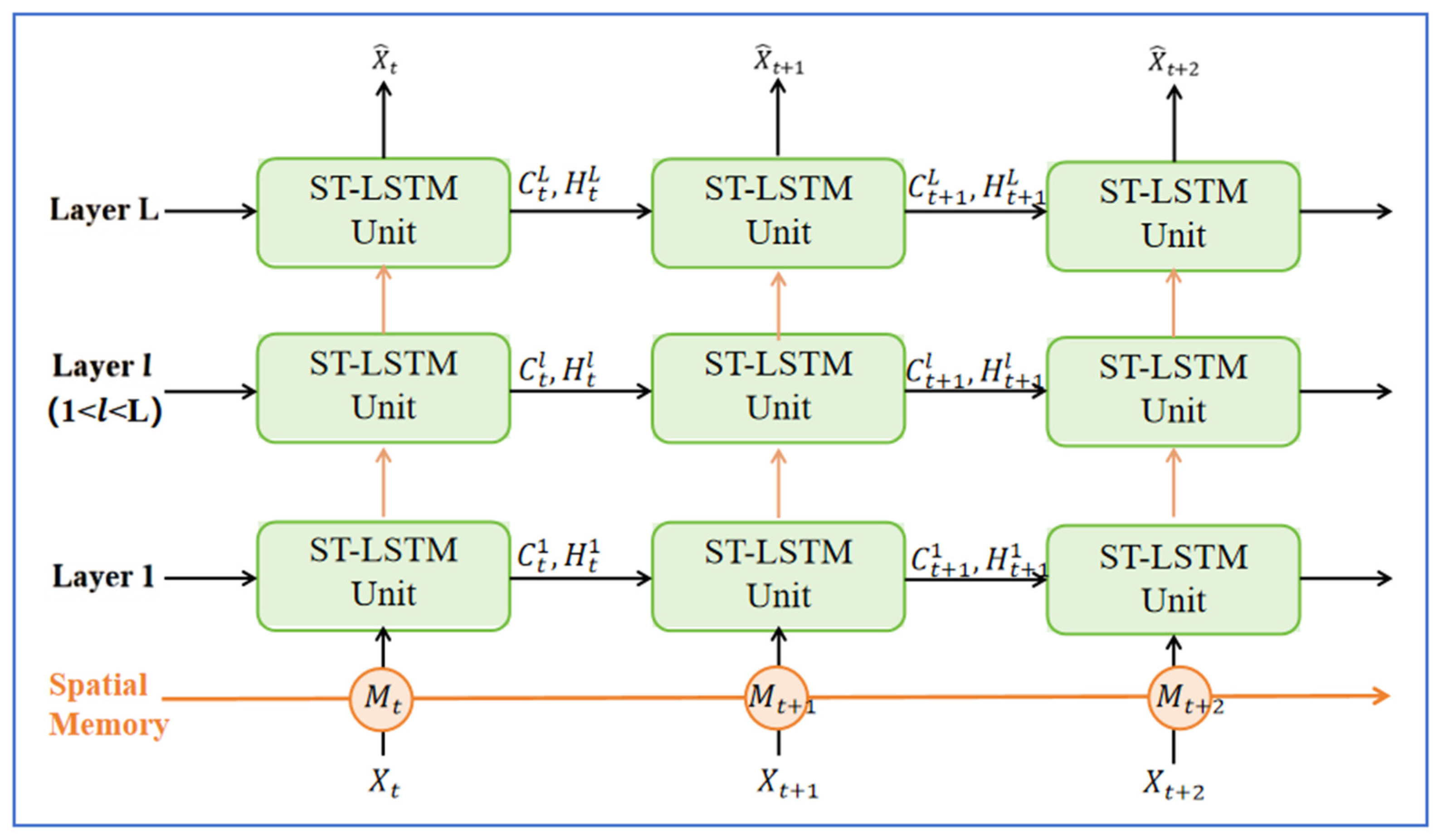
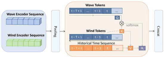
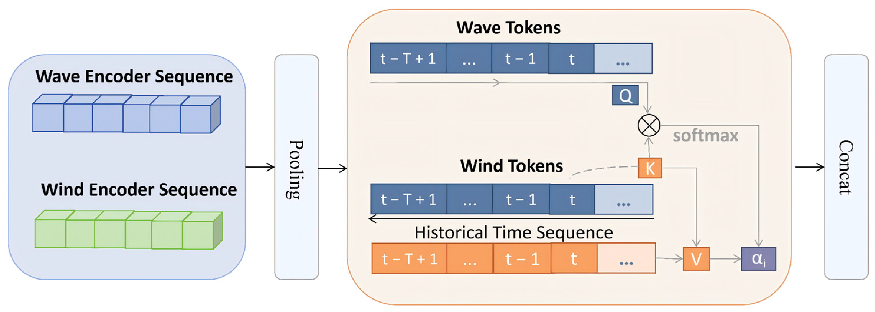
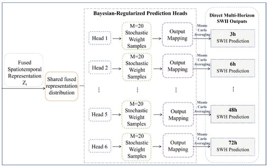
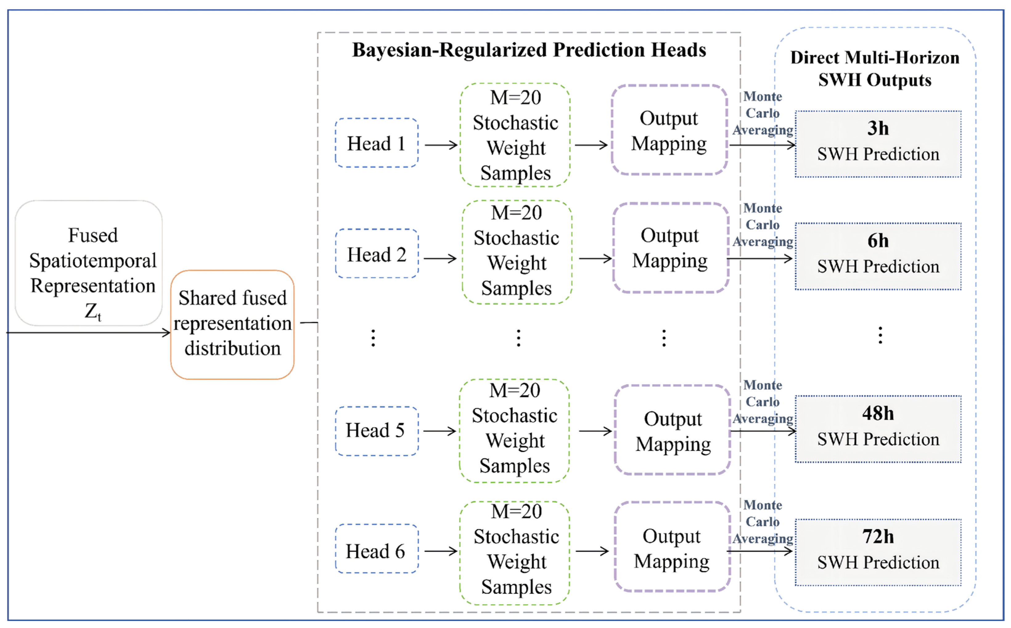
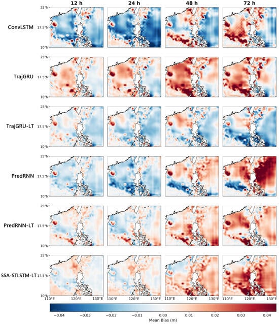
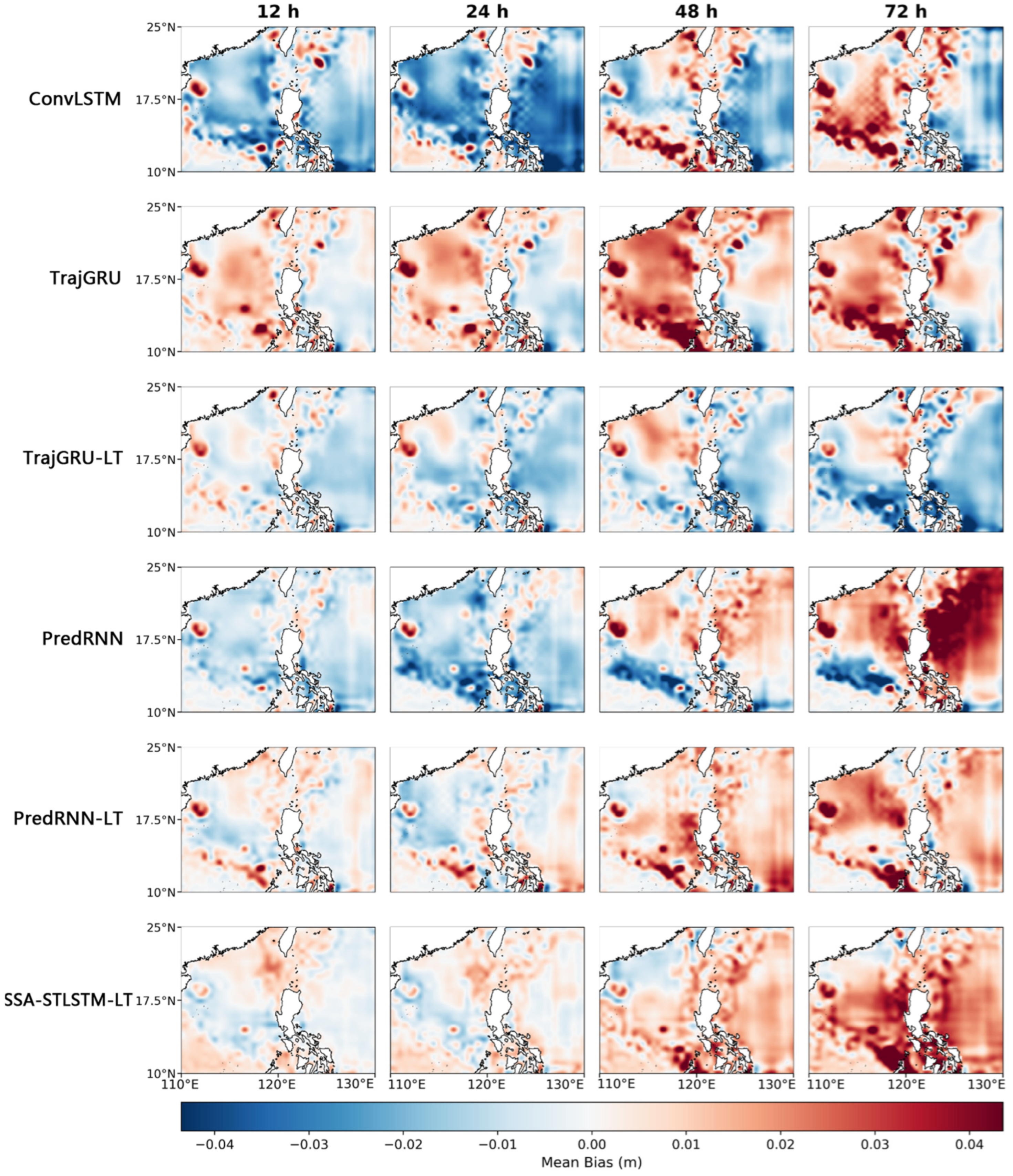
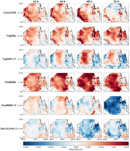
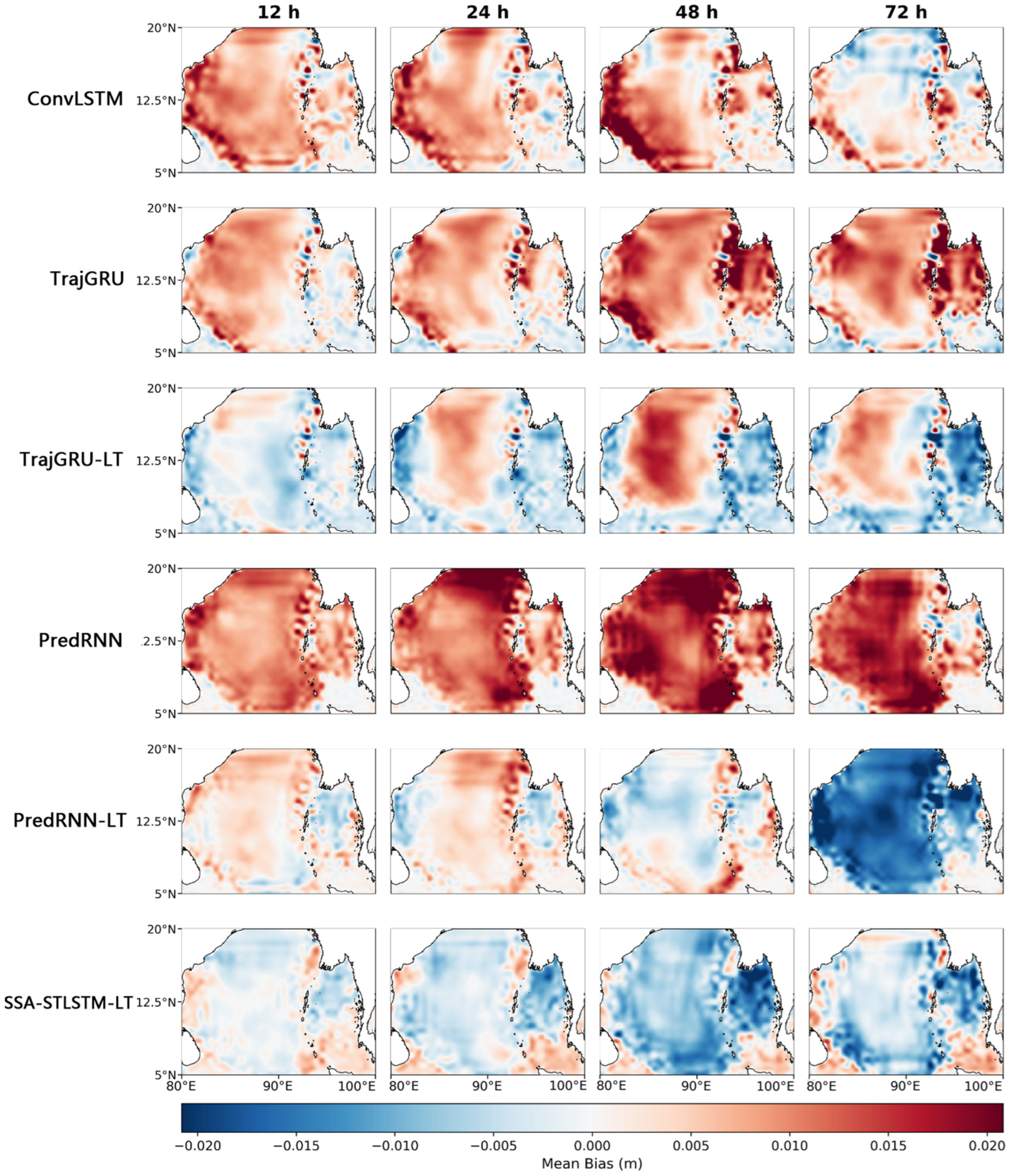
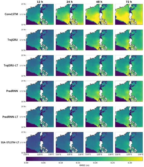
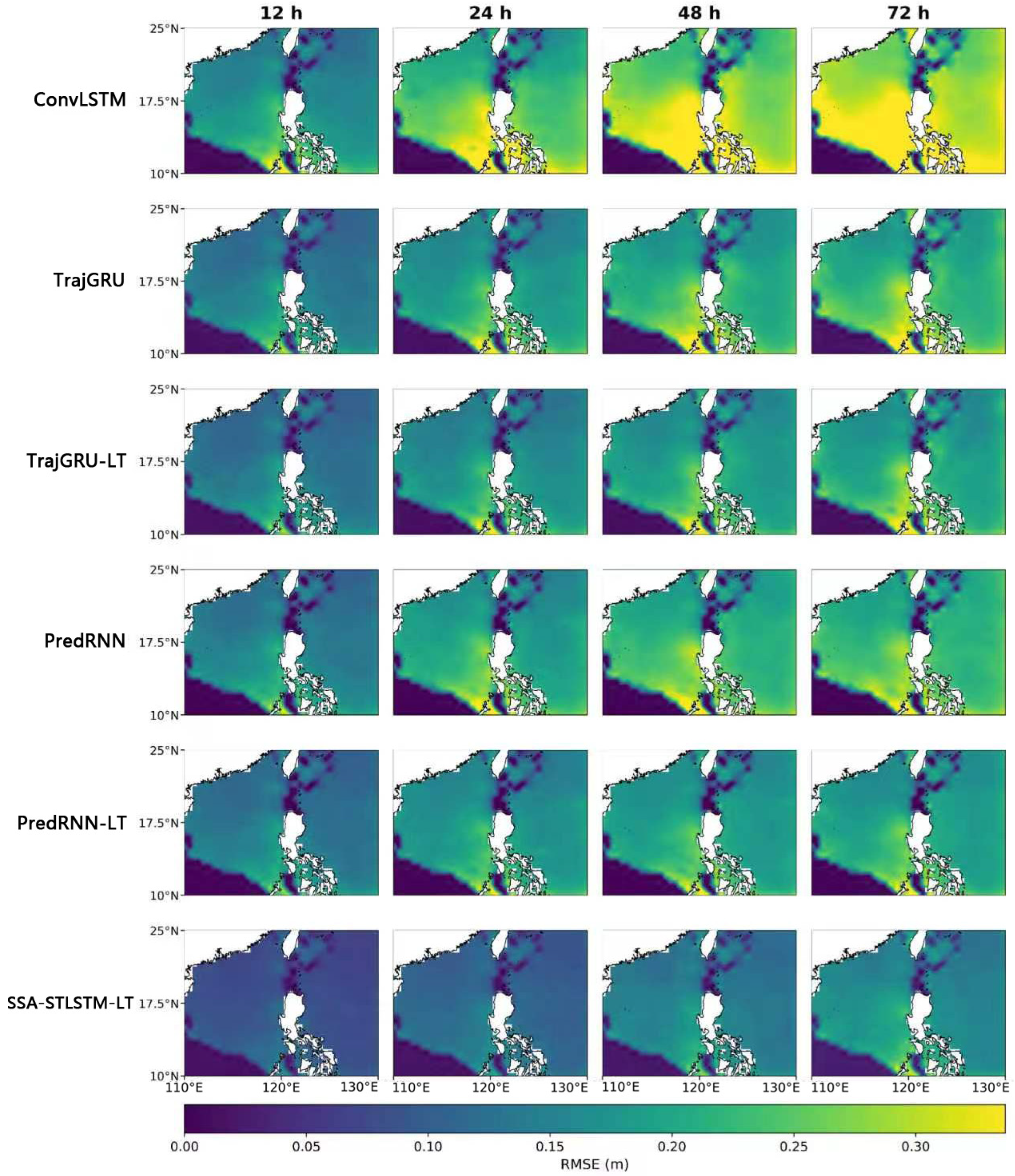
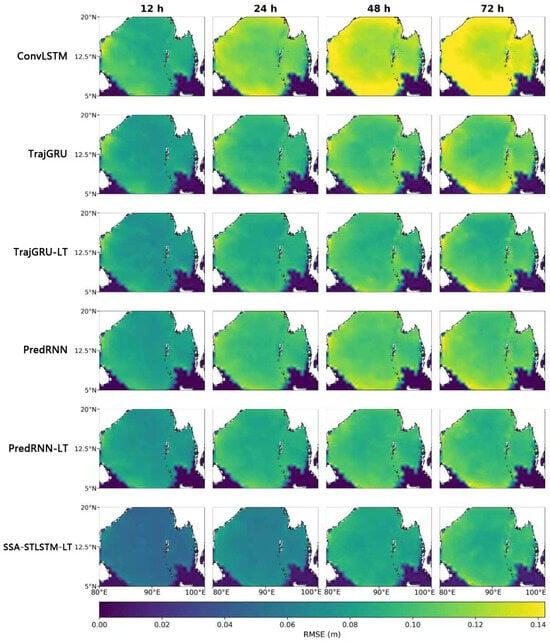
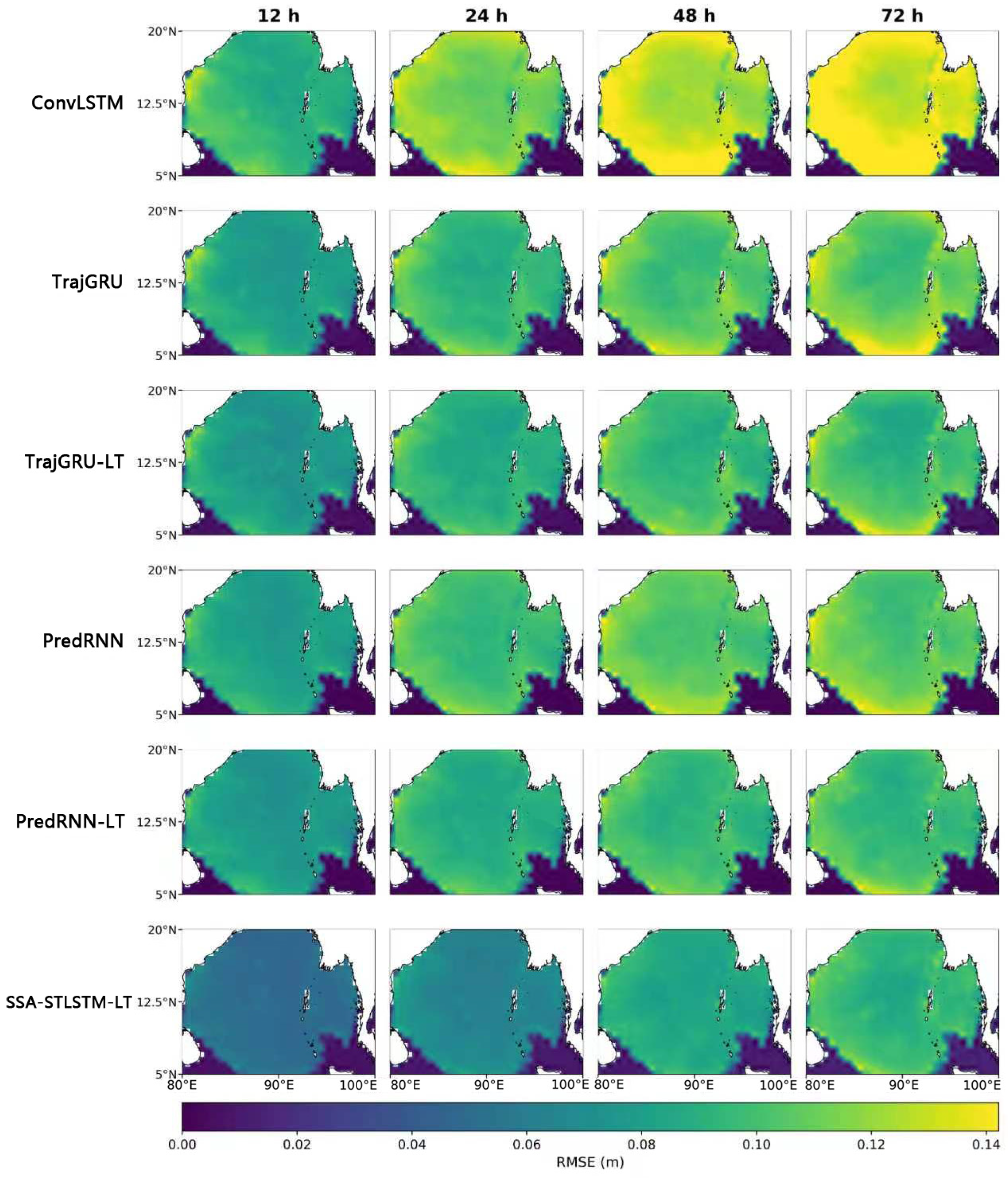
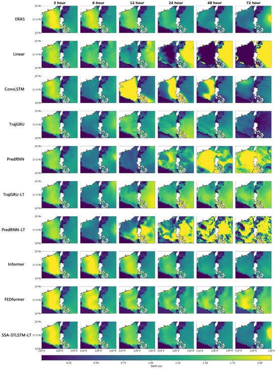
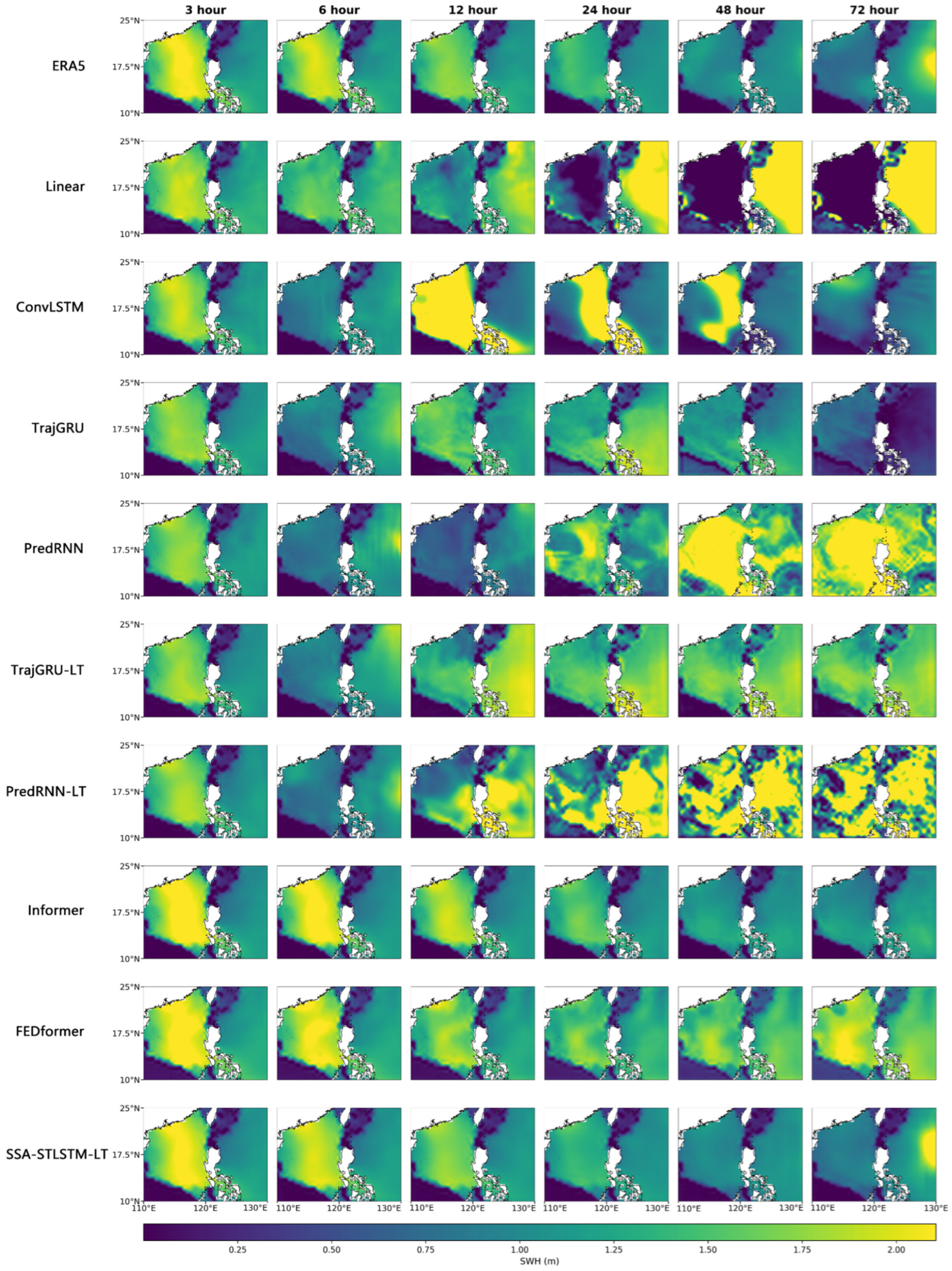
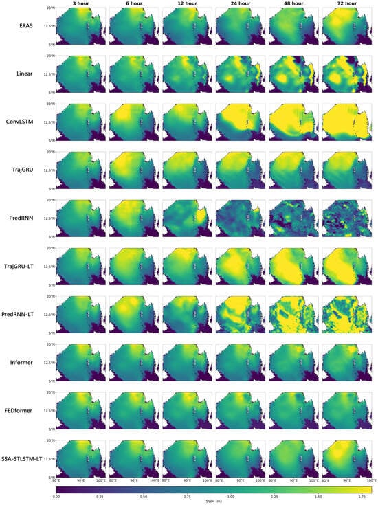
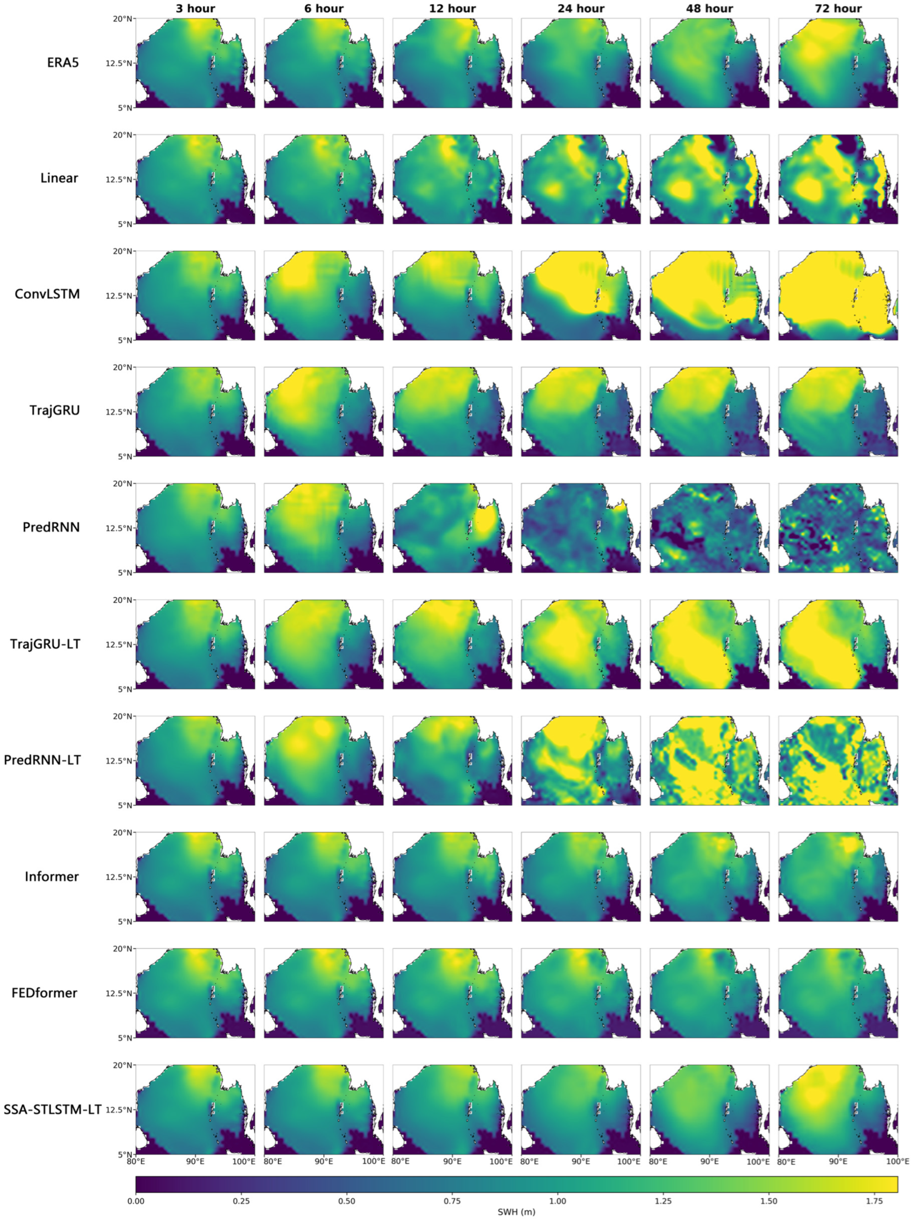
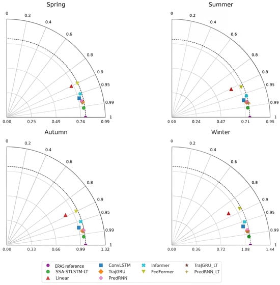
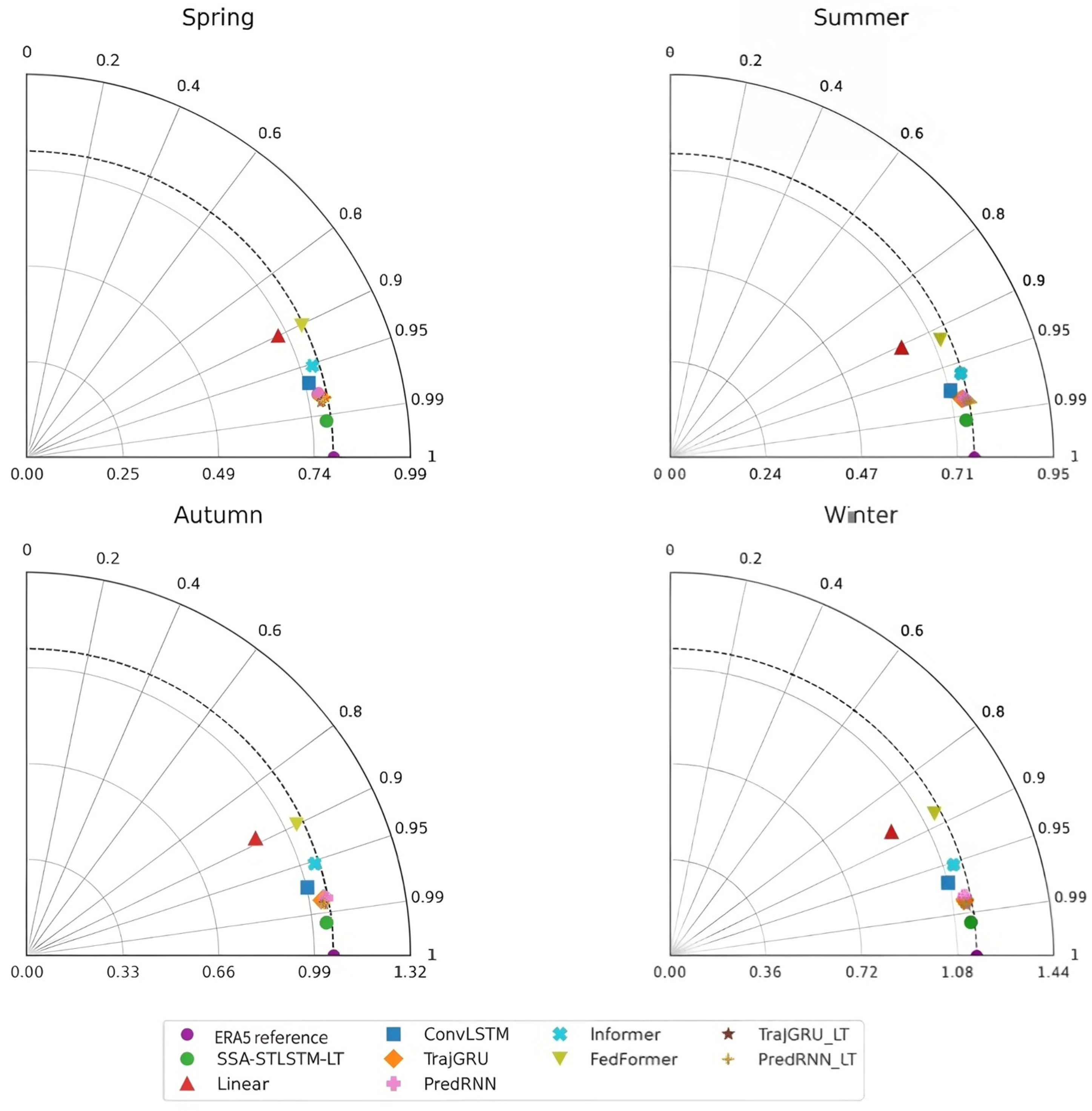
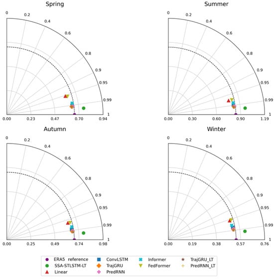
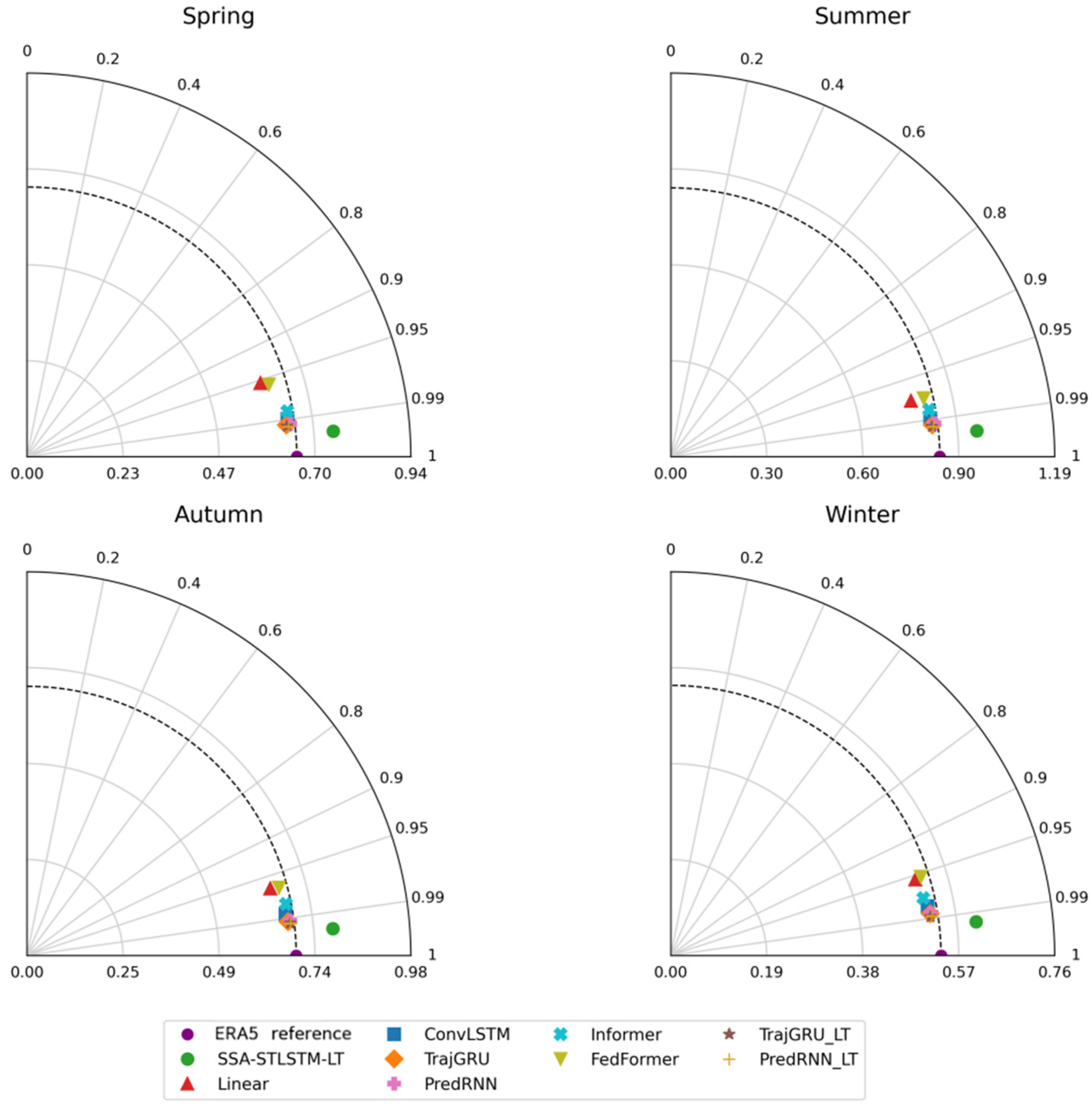
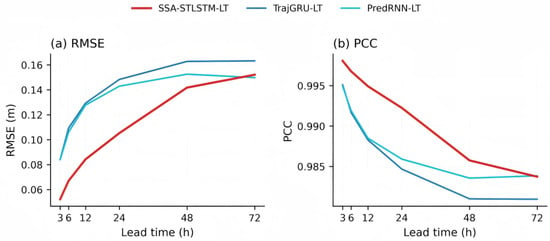
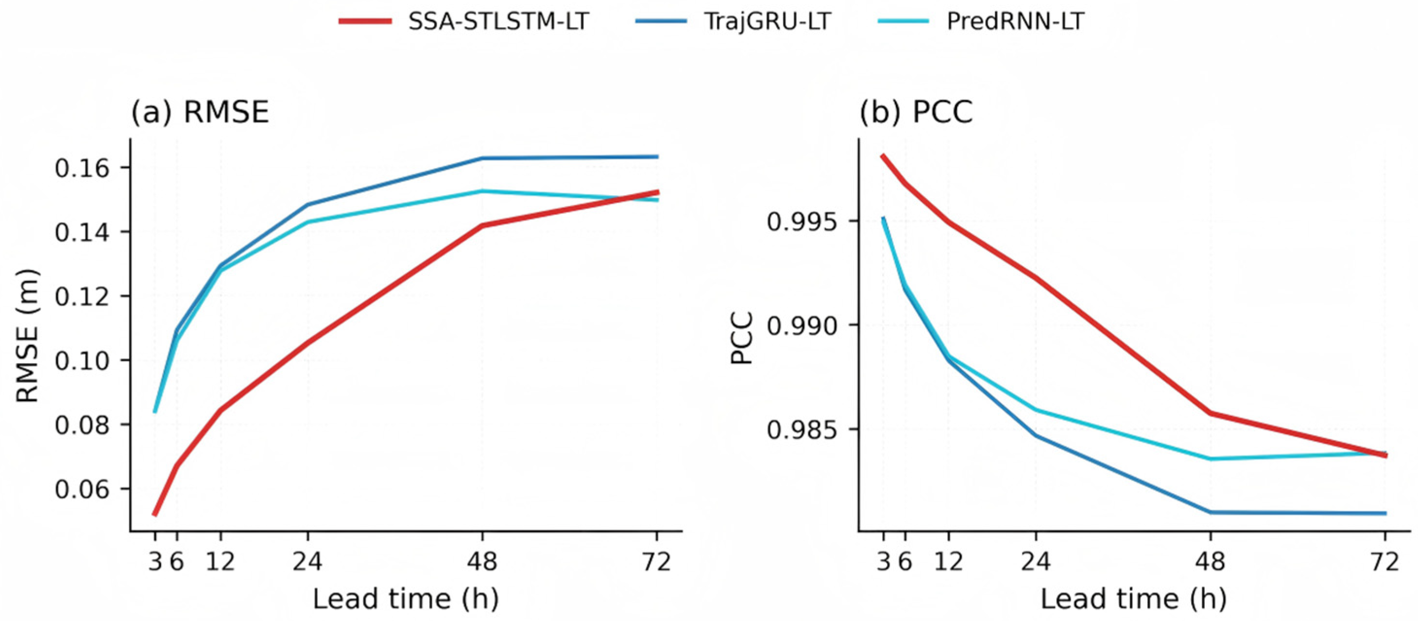
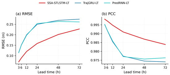
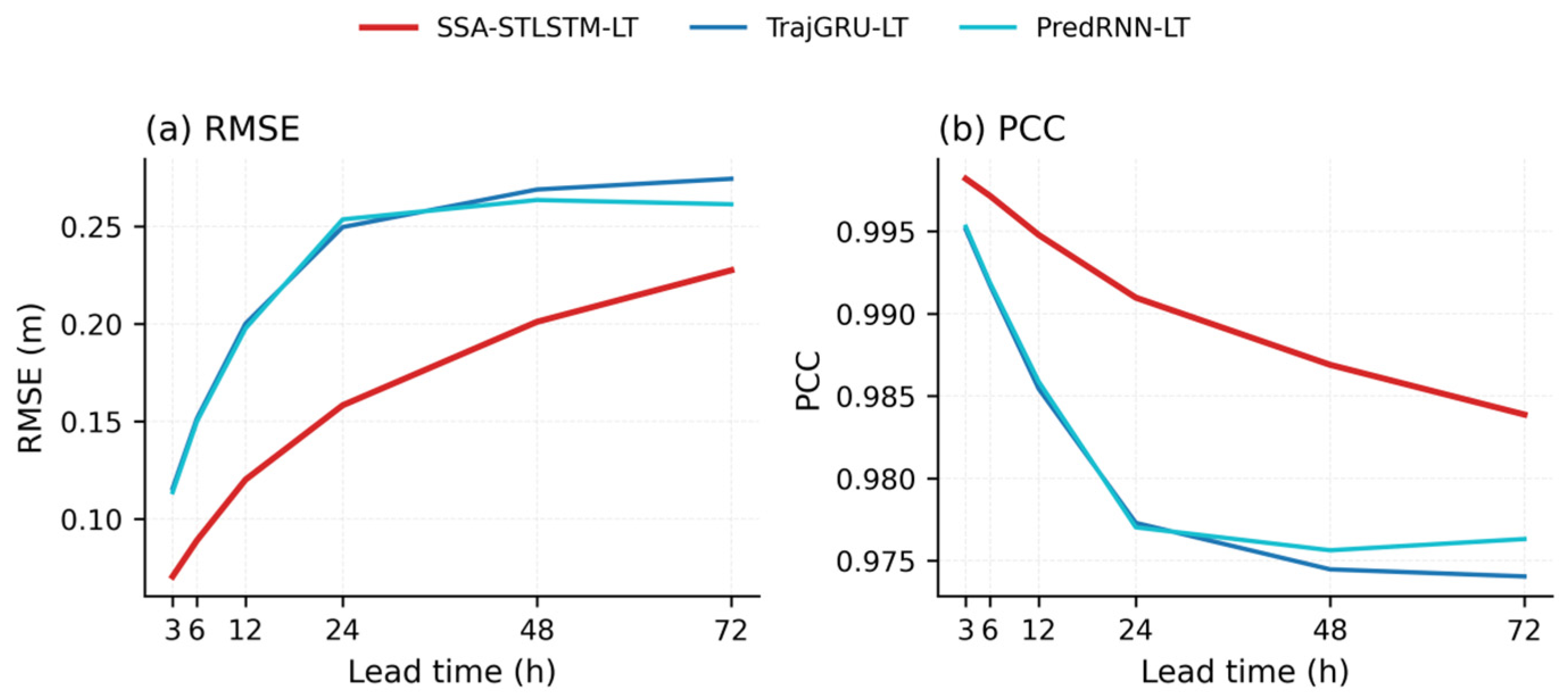
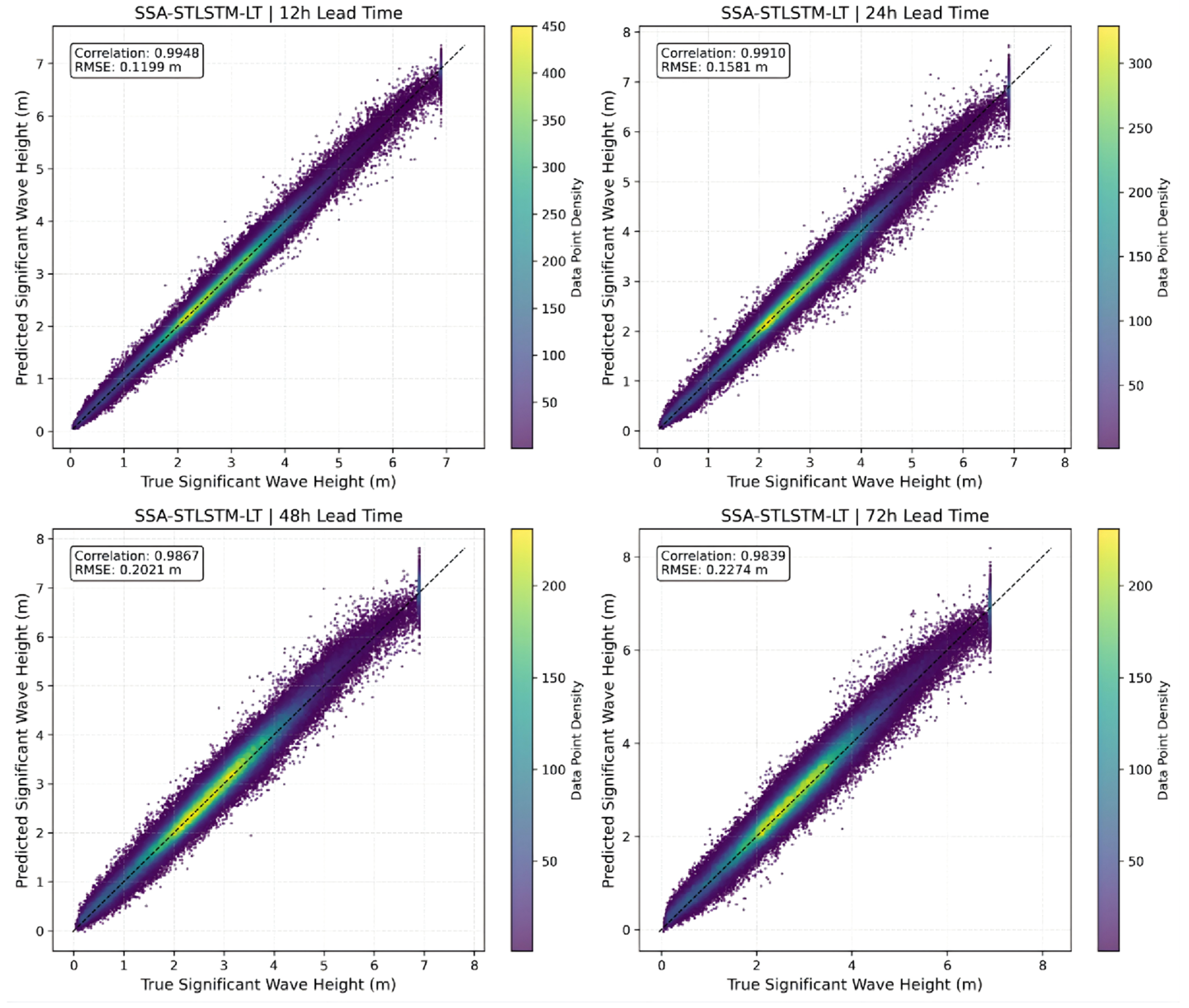
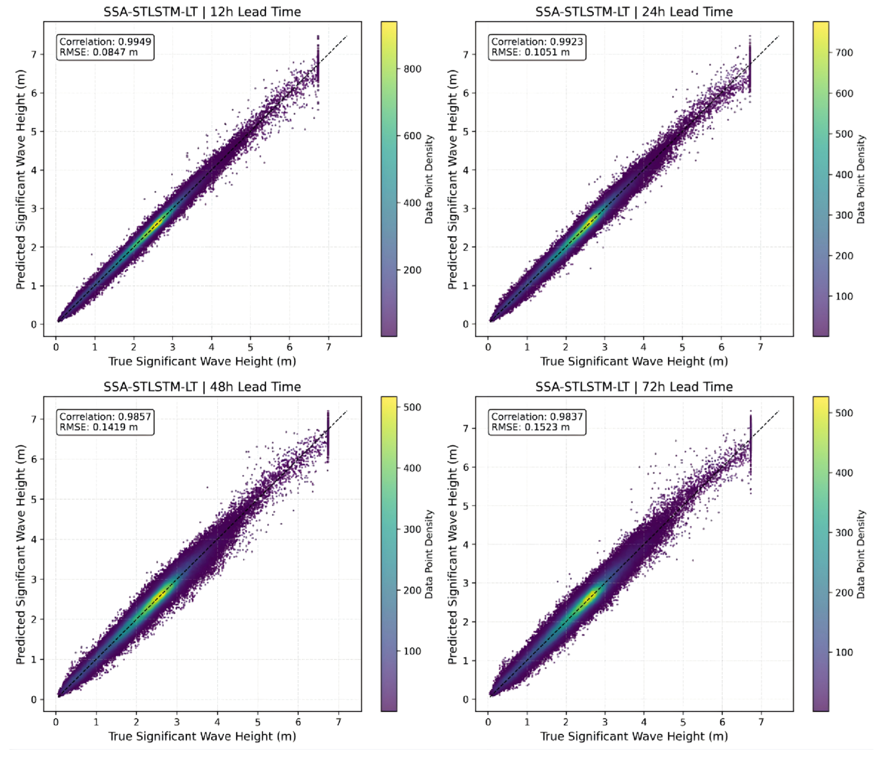
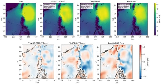
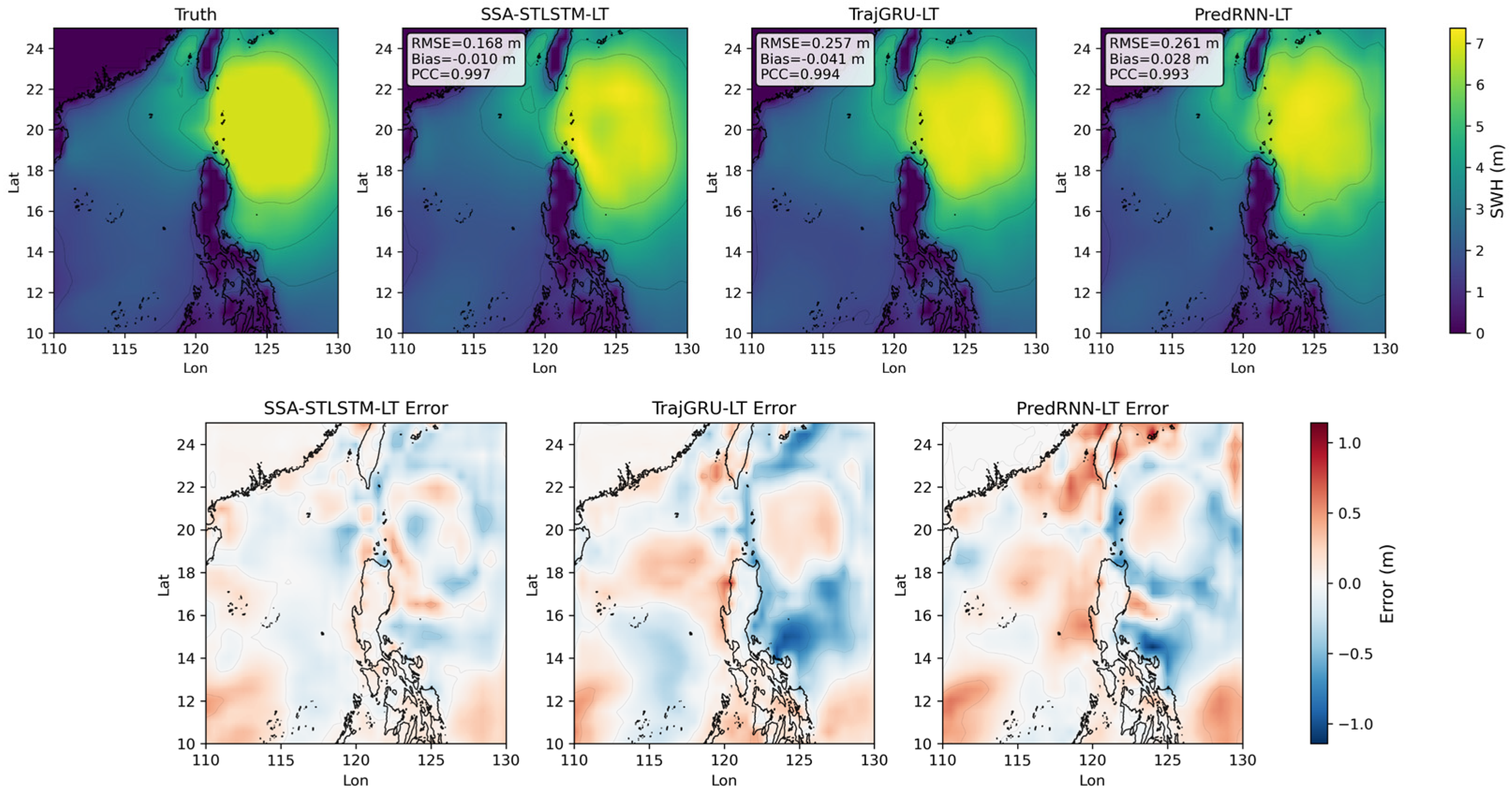
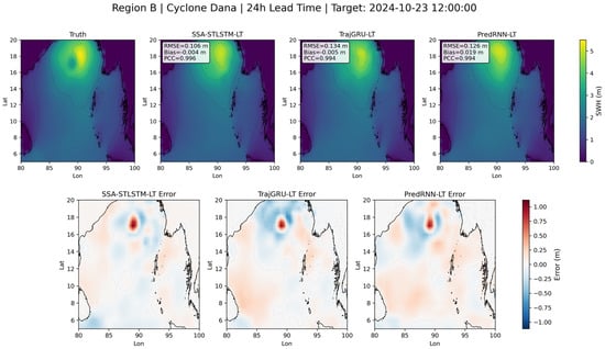
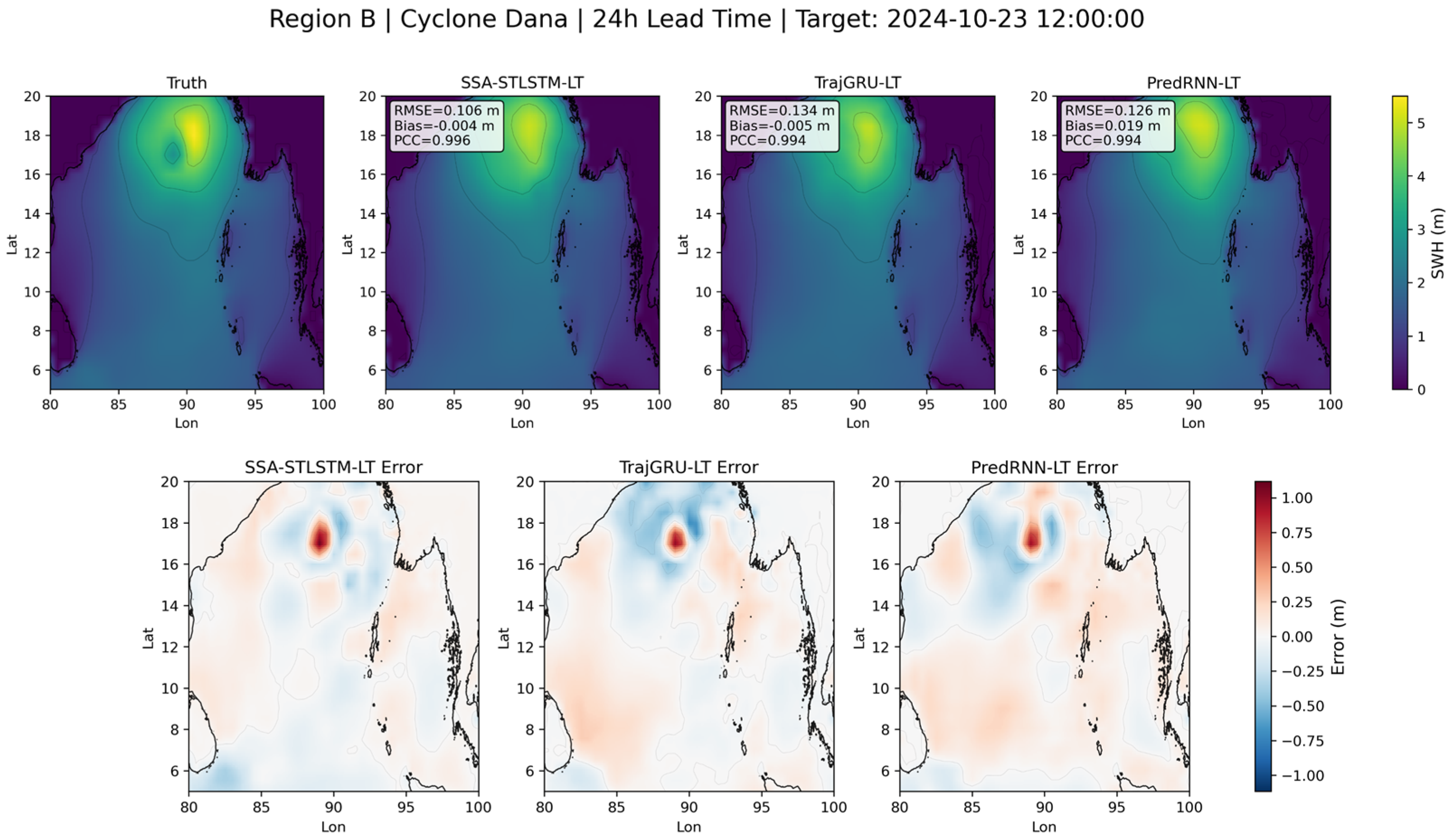
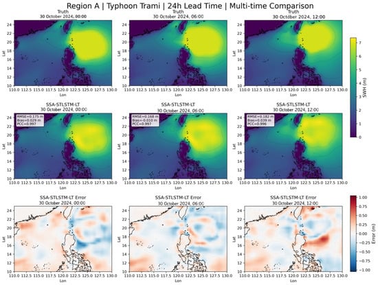
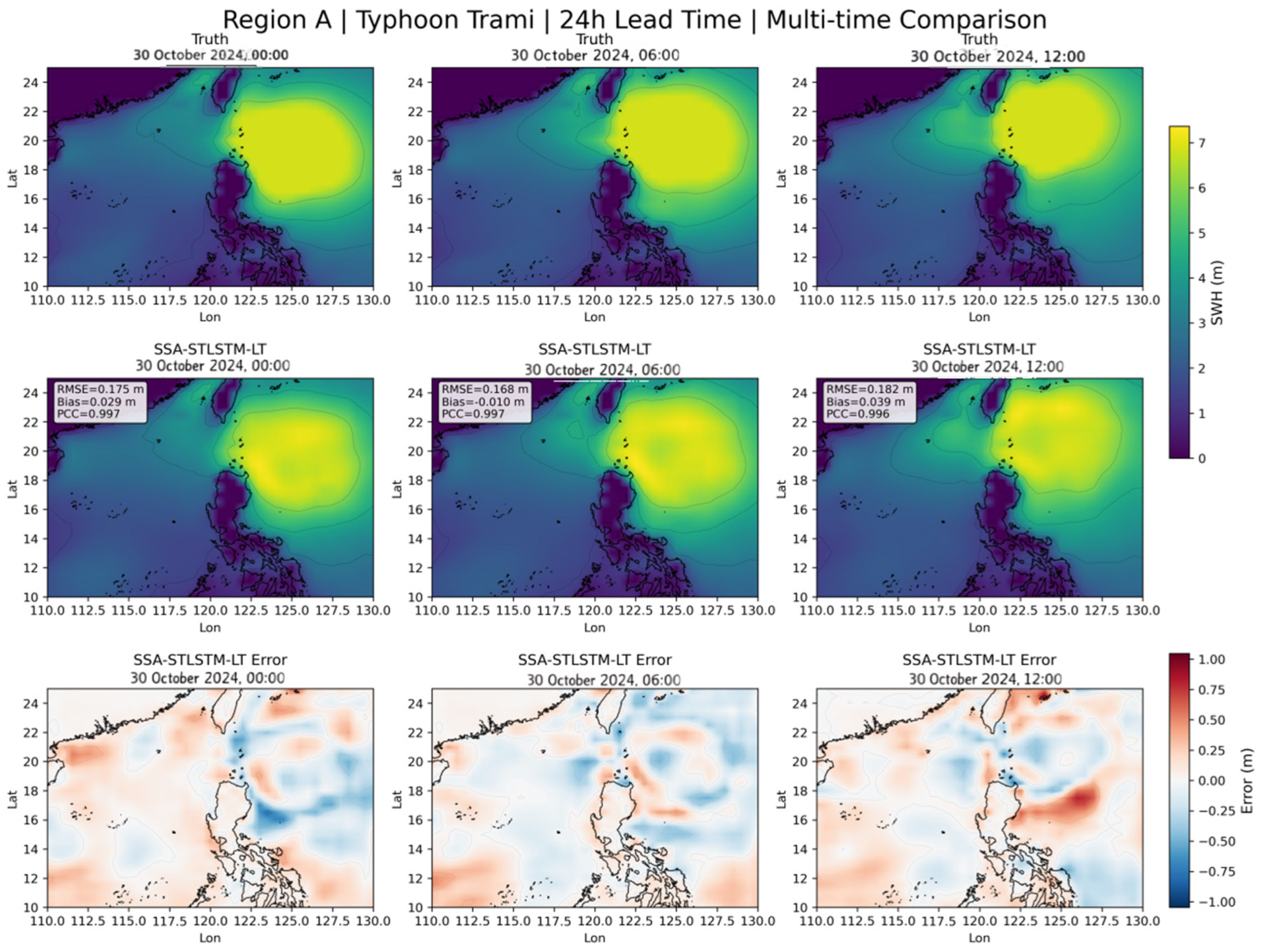
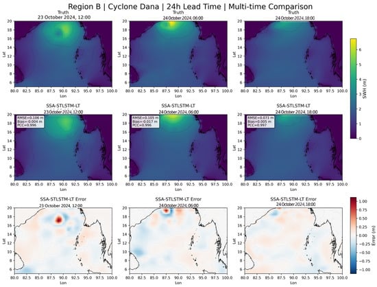
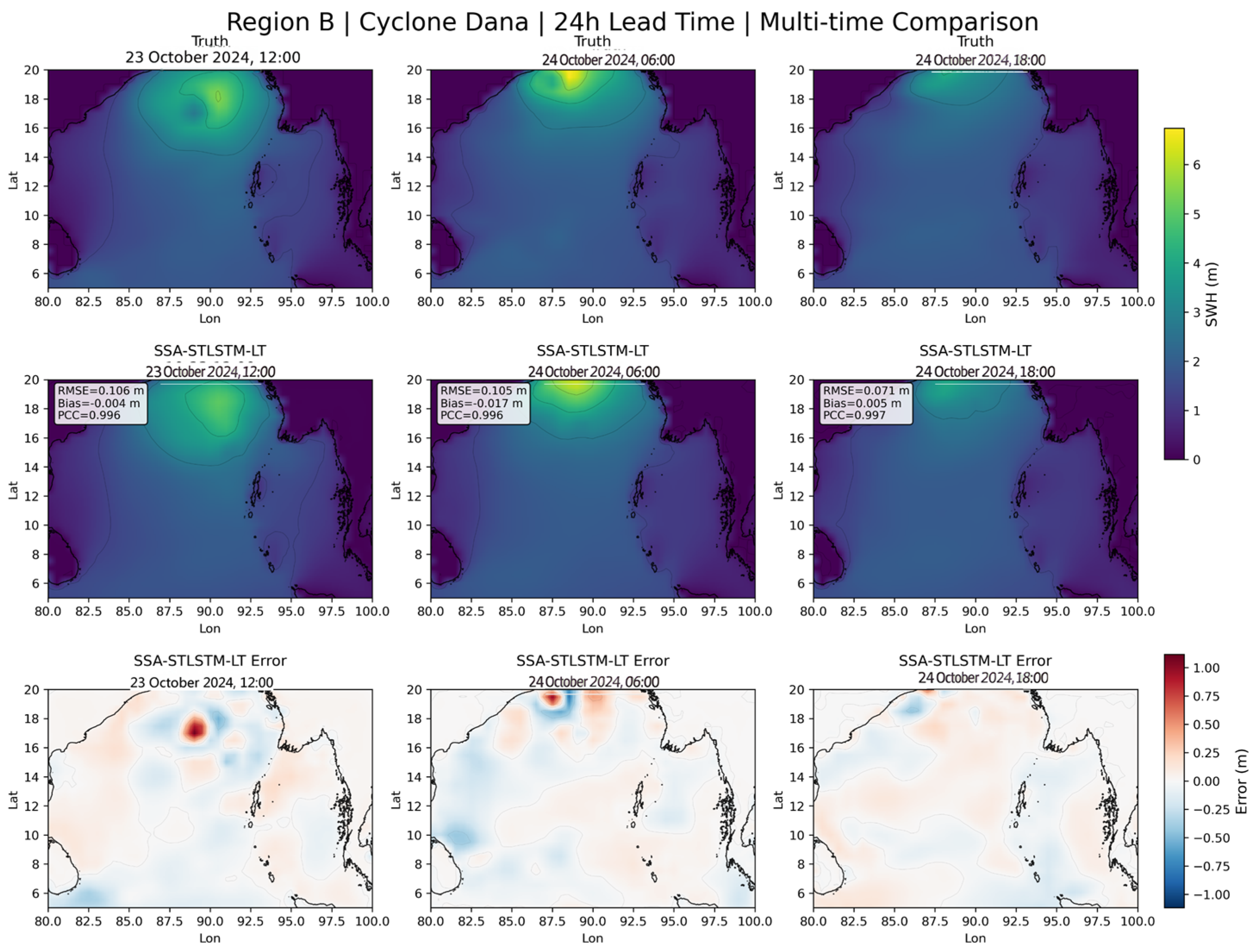
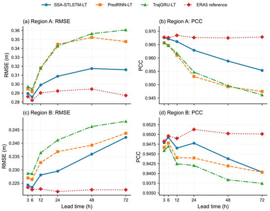
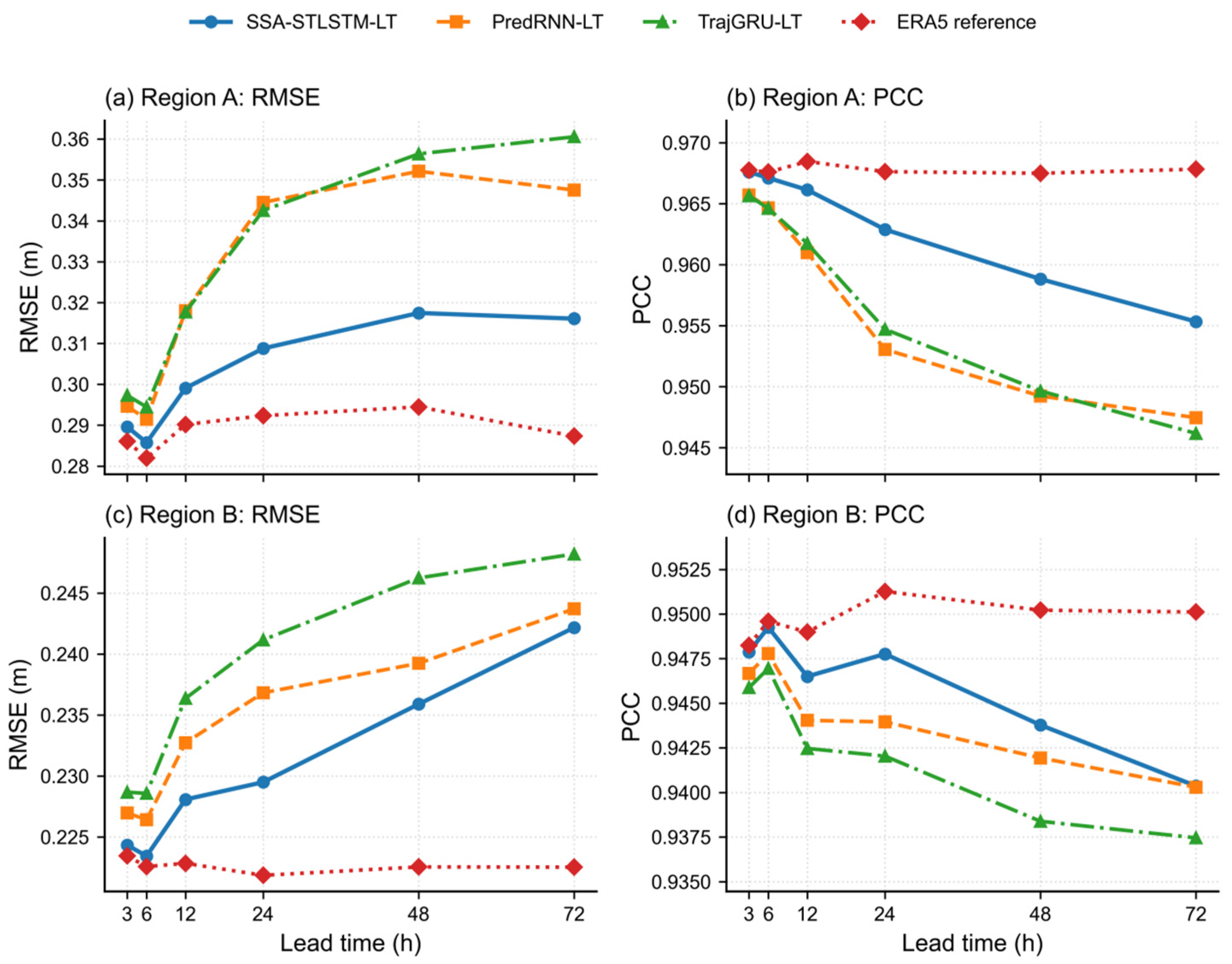
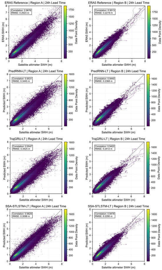
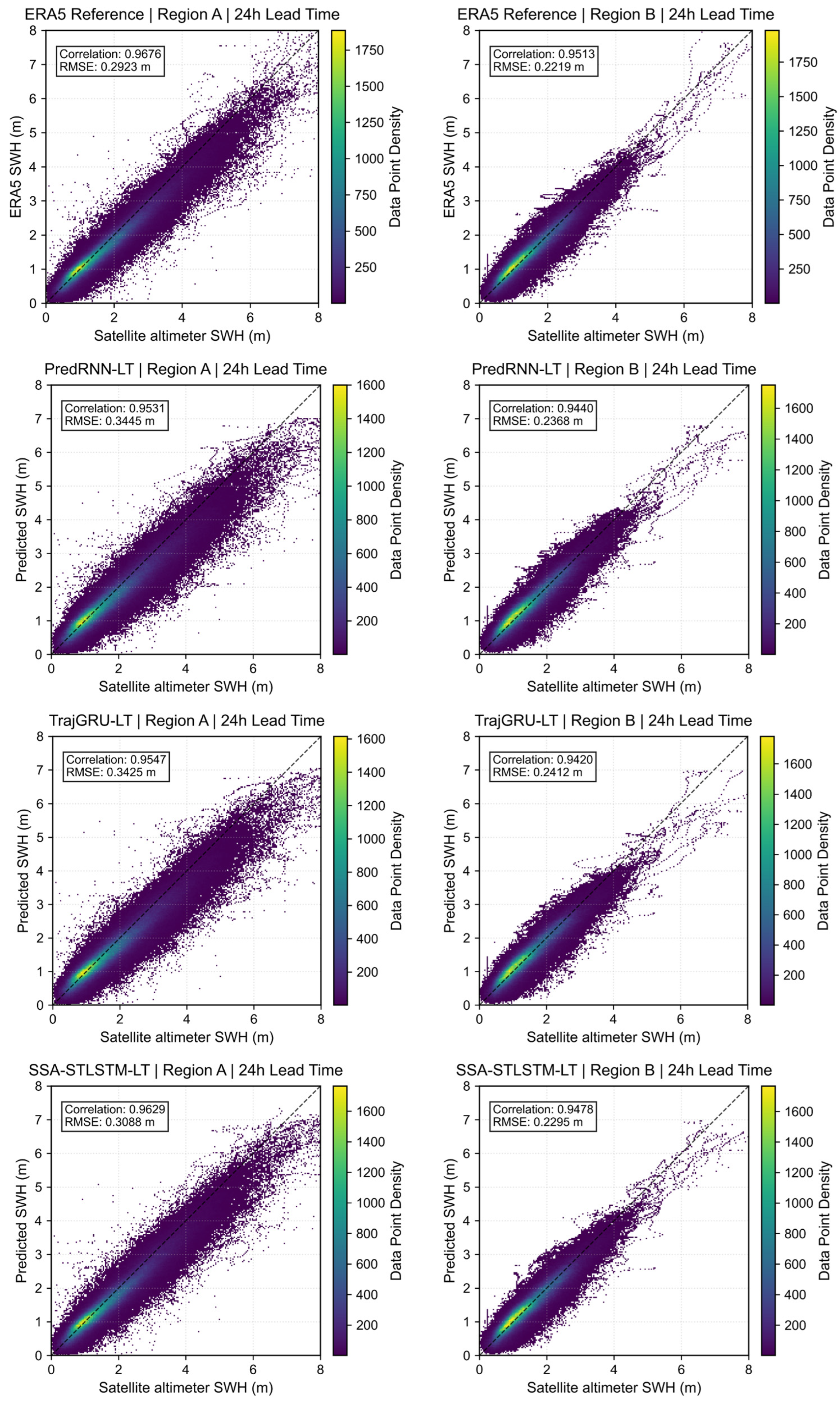

Disclaimer/Publisher’s Note: The statements, opinions and data contained in all publications are solely those of the individual author(s) and contributor(s) and not of MDPI and/or the editor(s). MDPI and/or the editor(s) disclaim responsibility for any injury to people or property resulting from any ideas, methods, instructions or products referred to in the content. |
© 2026 by the authors. Licensee MDPI, Basel, Switzerland. This article is an open access article distributed under the terms and conditions of the Creative Commons Attribution (CC BY) license.