


Abstract
Detecting anomalies in time-series data has significant implications in various domains, including the early detection of equipment and facility conditions in industrial settings and the identification of risk factors in financial markets. However, sensor-based time-series data obtained from real-world sites predominantly consist of normal patterns, with anomalies being extremely rare, resulting in insufficient data for model training. In this paper, we present a method that addresses the imbalance between normal and anomaly data by transforming time-series data into a structured sentence format and using a large language model to generate and augment diverse anomaly scenarios. The generated sentences are then converted back into time-series data and subjected to an internal validation process. This approach enables the construction of a broader range of anomaly data than existing techniques.The proposed method is designed for univariate, continuous valued time-series and is anticipated to serve as an effective data augmentation tool, with extension to broader domains left to future work.
1. Introduction
Anomaly detection in time-series is crucial across multiple domains, including industrial site monitoring and predictive maintenance. In practical industrial environments, time-series data are typically high-dimensional and collected from multiple sensors, with normal patterns greatly outnumbering anomalous events, which occur infrequently. This leads to ample availability of normal data, but significant scarcity of anomalous data. Such data imbalance and the rarity of anomalies are key challenges that hinder the development of effective detection models.
Models often struggle to differentiate normal from anomalous data under this imbalance. Prior work has largely relied on prediction-based and reconstruction-based methods, both of which face well-known limitations in capturing temporal dependencies and contextual anomalies and in setting clear decision thresholds [1].
Recently, several studies have utilized Large Language Models (LLMs) for time-series data prediction. Time-LLM approaches transform time-series data into textual prompts and feed them into a fixed LLM to address limitations commonly found in time-series forecasting. These models introduce reprogramming techniques that transform input series into sentences and employ the prompt-as-Prefix approach, thereby achieving higher forecasting accuracy than traditional specialized models, especially under few-shot and zero-shot learning conditions [2]. Another approach, the AnomalyLLM model, introduces a knowledge distillation technique where a pre-trained LLM serves as the teacher network to guide training of a student network. The AnomalyLLM framework leverages synthesized anomalies in combination with prototype signals extracted from normal time-series data and trains the student network to effectively discriminate between normal and anomalous patterns [3]. These LLM-driven studies demonstrate significant promise for enhancing anomaly detection effectiveness.
Furthermore, a range of data augmentation strategies have been explored to address the limitations associated with insufficient training samples in time-series forecasting, attracting substantial research interest. GeneRAting Time Series (GRATIS), Moving Block Bootstrap (MBB), DTW-Barycenter Averaging (DTW-BA), and related methods have been employed to augment time-series datasets, leading to measurable improvements in transfer learning and predictive model performance [4,5,6,7]. Notably, a number of studies have indicated that synthetic model-based techniques, including TimeGAN and Variational Recurrent Autoencoder (VRAE), learn inherent time-series patterns and generate a wide range of synthetic data to enhance the generalization capability of predictive models [8,9,10,11]. Nevertheless, most prior work remains tailored to domain-specific architectures, restricting their adaptability to novel domains. Thus, this research introduces LLM-AP, a new data augmentation-oriented framework that automatically converts time-series data into structured representations with anomaly type inference and domain context detection, employs LLM to synthesize anomalous scenarios through in-context learning with few-shot examples, validates results through a five-stage statistical process with Self-Refine feedback, and subsequently converts the validated results back into time-series data. The novel aspects and main contributions of the proposed approach are as follows.
- Overcoming the constraints of conventional synthesis methods: GAN and VAE-based models have been confined to domain-dependent and recurring anomaly generation, whereas LLM technology allows the creation of more authentic and varied anomaly scenarios to address these challenges;
- Implementation of validation procedures to ensure the reliability and quality of time-series data after augmentation: The generated anomaly scenarios undergo thorough verification, which assesses not only numerical accuracy but also logical coherence, intensity of augmentation, and overall realism;
- Reduced domain dependency within univariate series: LLM-AP automates prompt construction from the data itself, reducing reliance on per-domain manual configuration across univariate, continuous-valued time-series;
- Detector-agnostic augmentation: Generation is decoupled from detection, so the augmented dataset can train any downstream detector. This separates LLM-AP from task bound LLM backbones such as Time-LLM and AnomalyLLM;
To make the distinction between LLM-AP and prior approaches explicit in one place, Table 1 consolidates this comparison along four axes: the generation paradigm, the per-dataset training requirement, the degree of semantic controllability and human inspectability, and the presence of an explicit post-generation validation stage. Unlike TimeGAN, VAE-based, and diffusion-based generators, which must be trained on each target dataset and emit samples as opaque numerical tensors, LLM-AP employs a frozen, pre-trained LLM to synthesize anomalies that are first expressed in an inspectable structured text form and only then converted into numerical series. Unlike Time-LLM and AnomalyLLM, which embed the LLM in the inference model itself, LLM-AP uses the LLM solely as a controllable data generator whose outputs are screened by a five-stage statistical validation pipeline before entering the training set.
Table 1.
Comparison of Time-Series Anomaly Generation Paradigms and the Proposed LLM-AP.
Additionally, the organization of this paper is outlined as follows. Section 2 reviews previous research on time-series anomaly detection and the utilization of LLMs for time-series data, concluding with a focused discussion on data augmentation techniques. Section 3 describes the comprehensive architecture of the proposed LLM-AP framework, detailing the input time-series data preprocessing method, the LLM-driven anomaly scenario generation approach, and the multi-stage scenario verification process. Section 4 quantitatively evaluates the performance of the proposed method using the designated experimental setup and dataset, providing experimental outcomes in terms of data quality and model performance metrics. Finally, Section 5 discusses the conclusions drawn from the study and outlines potential directions for future research.
2. Related Work
2.1. Anomaly Detection
Anomaly detection in time-series data remains a critical and challenging task due to the infrequent occurrence of anomalies in sequential data, making them difficult to forecast. In this context, an anomaly is defined as a pattern in sequential data that diverges from expected normal behavior [12]. Detecting anomalies in industrial equipment and facilities is of major significance in industrial applications. Moreover, industrial environments are characterized by complex systems, and their sensor data is high-dimensional. In addition, most equipment and facilities operate under normal conditions, and anomalies occur only on rare occasions. A primary obstacle to accurate anomaly detection is the pronounced imbalance between normal and anomalous time-series data, mainly caused by the extreme scarcity of anomalous instances [13]. Consequently, a range of studies aimed at improving anomaly detection have been introduced to address these challenges.
Early research efforts have introduced both prediction-based and reconstruction-based approaches. For the prediction-based method, the approach entails forecasting the subsequent time point and then utilizing the error between the forecasted and actual values as an anomaly signal. For the reconstruction-based method, the process involves reconstructing the original time-series and then leveraging the discrepancy between the model’s reconstructed values and the input values to identify anomalies. Nevertheless, these methods present certain challenges. Prediction-based and reconstruction-based approaches are inadequate in capturing temporal dependencies and contextual anomalies, while reconstruction-based methods also tend to misclassify unrelated sections as anomalous, which do not pertain to actual anomaly events. This limitation is primarily due to the prevalent practice in existing studies of directly using reconstruction errors as anomaly indicators, despite reconstruction errors not providing a definitive boundary between normal and abnormal values. These shortcomings contribute to the failure in recognizing diverse normal patterns and elevate the probability of incorrectly flagging ambiguous segments as anomalies [14].
Recent research has sought to mitigate these challenges through various advanced methodologies. For instance, the AA-Forecast model stands out as a predictive framework that embeds anomaly patterns within the learning phase of the time-series prediction module, thus enhancing the accuracy in forecasting the likelihood of extreme occurrences [15]. Another accomplished approach integrates auto-encoder and regression techniques to not only predict subsequent values but also reconstruct input data, offering a more robust solution for early anomaly detection relative to traditional time-series anomaly detection methods, and has been proposed accordingly [16]. Moreover, a recently introduced method proactively identifies pattern shifts in time-series data, leverages these detected transitions as anomaly occurrence indicators, and quantifies anomaly severity in a staged fashion [17]. Despite such advancements in anomaly prediction, significant limitations persist. In addition, anomaly prediction continues to confront issues regarding generalizability, particularly when adapting models to new domains or responding to variations in sensor settings within existing measurement infrastructures, systems necessitating substantial investment in retraining or redeveloping models.
This paper introduces LLM-AP, specifically designed to overcome the constraints of current methodologies. LLM-AP reformulates time-series data into structured natural language templates before employing a Large Language Model (LLM) to generate and expand diverse anomaly scenarios, validate these scenarios, and translate them back to time-series format. This technique relies on data augmentation. The proposed method enables the creation of a wide array of anomaly scenarios and achieves superior flexibility for adaptation across a broad spectrum of domains.
2.2. Data Augmentation
In time-series anomaly detection, data augmentation techniques are employed to enhance model performance when training data is insufficient. Recent studies have introduced methods that generate diverse synthetic time-series data using approaches such as GRATIS, MBB, and DTW-BA to improve the effectiveness of global forecasting models, accompanied by a framework that leverages this synthetic data. By training models with both the augmented and original time-series data, or applying it for transfer learning with pre-trained models, these works demonstrate enhanced prediction accuracy even when data is limited [18]. Furthermore, research has systematically assessed and compared the effectiveness of nine distinct time-series data augmentation methods. Findings reveal that techniques like up-sampling or combining time-series data can improve model performance for prediction tasks involving small-scale datasets [19,20]. Moreover, there is active research on augmenting time-series data using generative models. Noteworthy among these is TimeGAN, which integrates the strengths of auto-regressive and GAN models to maintain the sequential properties of original time-series while generating realistic synthetic data [10]. Another study introduced mutation operations into the latent space of recurrent VAE to create synthetic anomaly time-series tailored for industrial control systems, combining them with original datasets and demonstrating improved anomaly detection by addressing class imbalance [21]. Additionally, a range of generative models, including variational recurrent autoencoders and recurrent VAEs, have been explored to model patterns in time-series data and produce new sequences [11].
More recently, diffusion-based generative models have emerged as a powerful alternative for time-series synthesis. By learning to reverse a gradual noising process, they generate high-fidelity sequences; Diffusion-TS, for instance, produces interpretable multivariate series via a decomposition-guided transformer, and diffusion-based frameworks have also been applied to time-series anomaly detection [22,23]. However, like GAN- and VAE-based methods, diffusion models require dataset-specific training and operate in a learned latent or signal space, which limits their controllability over semantically specified anomaly types and their transfer across domains.
Recently, research applying Large Language Models has been introduced to the domain of time-series data anomaly detection and forecasting. While in computer vision, large pre-trained models are extensively applied across diverse tasks and domains, such universal models have not been widely adopted for time-series anomaly detection, primarily due to limited data availability. Nonetheless, the advanced sequence analysis and inference abilities of LLMs have spurred a variety of studies investigating their use for time-series data [24].
2.3. LLM and Its Applications
Recently, research leveraging Large Language Models has gained attention in the area of time-series anomaly detection and forecasting. In computer vision, it is common for a single large pre-trained model to be applied across diverse domains or tasks. Conversely, the development of universal models for time-series anomaly detection remains restricted, primarily due to challenges such as data scarcity. Nonetheless, LLMs exhibit sophisticated sequence pattern recognition and inferential abilities, leading to multiple studies investigating their applicability to time-series data [24]. Among various approaches to time-series anomaly prediction, the Time-LLM model introduces a method that transforms input time-series data into textual prompts, thereby enabling the use of pre-trained language models without necessitating retraining, and presents a framework for enhancing the contextual information of time-series. This method submits the transformed prompts to the LLM and subsequently maps the LLM’s output back to the time-series forecasting values. Empirical results show that the proposed Time-LLM model delivers superior performance compared to other time-series forecasting models, especially in few-shot and zero-shot settings where training data is limited. Consequently, ongoing research seeks to integrate LLMs into time-series prediction by combining them with various architectures to propose enhanced hybrid models [2]. Despite this, some studies report mixed or critical assessments of LLM-based methods for time-series data. Specifically, recent work indicates that removing or substituting the LLM module in existing LLM-based time-series anomaly forecasting models often leads to minimal or no loss in performance, and in many instances, even results in improved outcomes. Additionally, there are cases where models trained entirely from scratch outperform those based on pre-fine-tuned LLMs, with findings suggesting that LLMs may fail to effectively capture the temporal dependencies essential for time-series analysis and that the purported strengths of LLMs may be overstated in settings constrained by limited data availability. These results highlight the challenges of deploying domain-agnostic, general-purpose LLMs as effective anomaly forecasting models for time-series data [25]. Thus, drawing on these insights, further research is necessary to fully exploit the strengths of LLMs while adapting them to the specific characteristics of time-series data.
Importantly, this critique concerns the use of LLMs as forecasting or detection models, in which the LLM must itself capture temporal dependencies [25]. LLM-AP does not place the LLM in that role: it uses the LLM only as a controllable generator of synthetic anomaly scenarios from natural-language specifications. This task draws on the LLM’s language understanding, in-context generalization, and ability to produce semantically specified variations including anomaly types scarce in the source data rather than on its numerical forecasting accuracy. The reliability of the generated data is then ensured by the downstream statistical validation pipeline rather than by the LLM alone. The questionable forecasting ability of LLMs is therefore not a prerequisite for the effectiveness of our augmentation framework.
LLM research encompasses not only forecasting but also anomaly detection and data augmentation. Among recent approaches, AnomalyLLM employs a pre-trained LLM as a teacher network and introduces a knowledge distillation structure where the student model emulates the teacher. Within the knowledge distillation framework, both prototypical signals from normal time-series data and representations of anomalous scenarios are provided, enabling the student model to distinguish effectively between standard and anomalous patterns. This model achieved superior accuracy compared to existing techniques across more than 15 real-world datasets [3]. Although LLM-based anomaly detection for time-series data is still in an early stage, advances in LLM capabilities are expected to facilitate the development of more robust and scalable research in this domain [26].
LLM-AP differs from prior work in three respects. Generative augmentation models such as TimeGAN, recurrent-VAE methods, and diffusion based generators must be trained on each target dataset and can only reproduce the patterns contained in that training distribution. LLM-AP instead augments through in-context learning with a frozen LLM, so no per-dataset training is needed and anomaly subtypes that are rare or absent in the source series can still be synthesized [5,11,21]. It also differs from recent LLM-based time-series methods in how the LLM is used: Time-LLM reprograms a frozen LLM into a forecasting backbone, and AnomalyLLM uses an LLM as a teacher to distill a dedicated student detector so in both the LLM is part of the inference model and is tied to a specific task head. LLM-AP instead uses the LLM solely as a controllable data generator, decoupled from detection, so the augmented data can train any downstream detector. Generation is then paired with a five-stage statistical validation pipeline and a Self-Refine loop, so the realism and type fidelity of each synthetic anomaly are checked before it enters the dataset, a safeguard that latent-space generators lack [2,3].
Beyond prompting general-purpose LLMs, a parallel line of work develops time-series foundation models—large models pretrained on broad collections of time-series. Examples include Chronos, TimesFM, and Moirai for forecasting, and MOMENT, which additionally supports anomaly detection. While these models primarily target prediction and representation rather than data augmentation, they reflect the same trend toward general-purpose, transferable time-series models that motivates LLM-AP [27,28,29,30,31].
3. LLM-AP: Domain-Adaptive Anomaly Analysis
3.1. Model Framework
This paper introduces a novel data augmentation structure designed to enhance the anomaly detection performance for time-series data. The proposed approach transforms time-series data into structured natural language sentences interpretable by LLM, augments them using LLM with various anomalies and user-supplied information, and subsequently reconstructs the structured sentences back into time-series data, producing a format suitable for direct model training. Figure 1 presents a graphical depiction of the proposed structure, which is organized into three main stages and subdivided into four specific stages. The initial stage transforms the input time-series data into structured natural language sentences formatted for LLM utilization. This requires defining a structured template for the sentences beforehand. The structured sentence format incorporates variables such as user-provided domain information, typical and anomalous data states, sensor types, data observation intervals, numerical value ranges, and trend changes. User-entered information supplies context relevant to the domain or facilitates the LLM’s understanding of the data. The set of variables included is categorized into mutable variables, which may be altered during data augmentation, and immutable variables that remain unchanged and are not augmented during the augmentation phase, both managed via LLM processing. For instance, when converting time-series data into natural language structured sentences such as “Sensor x gradually increased from value a to value b over n seconds,” the resulting example would be “Sensor A gradually increased from value 1 to value 5 over 5 s.” In this context, components like “sensor x n seconds” are immutable variables that are not augmented, while ‘a’ and “b” represent mutable variables subject to augmentation. This structured sentence format optimizes LLM’s ability to interpret and modify data, laying the groundwork for generating diverse anomaly scenarios.
Figure 1.
LLM-AP Framework Overview.
The second stage involves utilizing LLM to augment data by transforming input data into structured sentence format containing anomaly data. The structured sentences produced in the prior stage serve as inputs, maintaining their sentence structure while incorporating both normal and anomaly scenario examples. The anomaly example types provided are categorized, and a concise description of the trend for each type is included to produce realistic anomalies. The included explanations are crafted using a prompt strategy that allows the LLM to clearly distinguish between normal and anomaly scenarios. Adequate context, details, and examples are supplied at the prompting phase to ensure the generated augmented scenarios authentically reflect actual time-series dynamics and meanings.
Additionally, the proposed augmentation method incorporates anomalies likely to appear in real-world settings, which aids the detection model in identifying diverse anomaly phenomena. In the concluding procedure of the second stage, the enhanced anomaly data, after being returned to the time-series format, is rigorously validated and integrated with the original dataset to create the final dataset. The structured sentence, augmented with anomaly content, is processed to recover variables, time metadata, value intervals, temporal patterns, and other relevant elements, converting them from natural language back to time-series data. Restoration relies on the structured sentence template set out in the initial phase and requires extracting each variable from the sentence and reconverting this information into time-series data. For instance, the phrase “Gradually increased from 10 to 11, 13.5, 15, … 20 over 30 s” can be transformed into sequential time-series data with values consistently increasing at a stable rate.
During the final stage, a systematic five-step verification protocol is performed to quantitatively assess and ensure the reliability of the augmented anomaly time-series data. Upon completion of this verification process, the anomaly time-series data is merged with the original input to create a final dataset containing a balanced ratio of normal and anomaly instances. This final dataset serves as the foundation for model training, enhancing the model’s detection capabilities.
Figure 2 depicts the comprehensive workflow of LLM-AP, which is the method introduced in this study. LLM-AP facilitates anomaly data augmentation tailored to a broad spectrum of time-series domains that are often challenging for traditional numerical-based augmentation techniques. Notably, it enables the adaptable expansion of LLM-based data augmentation, employing structured sentence structures to simultaneously improve the diversity and realism of datasets for detection model training.
Figure 2.
LLM-AP Flow Diagram.
The key design principle of LLM-AP is to eliminate manual prompt engineering. Unlike existing approaches, where users must describe time-series characteristics directly in natural language, LLM-AP automatically extracts all necessary information from the data itself. Anomaly types are inferred through score-based classification, which analyzes z-scores, mean deviation, variance ratio, gradient magnitude, and monotonicity patterns in the signal characteristics of each anomaly window. Domain context is detected from the dataset’s file path structure, mapping category directories and filename keywords to domain descriptions and sensor types with appropriate units. Examples are automatically selected from normal and anomalous windows within the dataset itself. Thanks to this automation, LLM-AP can process arbitrary time-series datasets without manual data annotation, addressing a practical limitation of existing LLM-based augmentation approaches that required domain expertise for prompt configuration.
Moreover, the majority of current time-series data augmentation methods are typically designed based on patterns or time-series distributions relevant to specific domains. Such methods face limitations, as their effectiveness may decline with domain changes or may necessitate complete model redevelopment. Additionally, given the varied interpretation and representation of time-series data across domains, the applicability of current augmentation techniques remains restricted. In contrast, the LLM-based augmentation framework introduced in this paper reduces domain dependency by transforming time-series data into structured natural language sentences and exploiting the LLM’s language generation capabilities to produce diverse augmentations. Unlike previous approaches sensitive to domain-dependent interpretations, the same pipeline can be applied across univariate, continuous-valued datasets without per-domain structural redesign, owing to a consistent representation.
3.2. Time-Series Data Pre-Processing
To facilitate efficient processing by LLM, the original time-series data is transformed into a structured sequence of natural language sentences. The sentences produced through this transformation are carefully refined to maintain clear content, contextual consistency, and accuracy in relation to the underlying data. Inputs that could introduce unnecessary noise or that are ambiguous and challenging to interpret are systematically omitted. Lengthy or overly complicated sentences are also avoided, as they can result in the generation of sentences containing inaccuracies. Instead, concise and relevant phrasing is prioritized, and sentences are formulated in conjunction with user-provided information. The standardized sentence structure adopted by LLM-AP does not deliberately alter the sentence format nor utilize varied styles of expression. Instead, by selectively modifying semantic elements within each sentence—such as parameter values or trend durations—the system ensures diversity in generated sentences while preserving uniformity in format, thereby supporting the generation of coherent anomaly scenarios.
Figure 3 provides a schematic overview of the initial step in the LLM-AP pre-processing workflow. LLM-AP contributes to reducing the likelihood of inaccurate sentence generation by enforcing standardization in both sentence structure and time-series reconstruction, while retaining variation within a stable sentence framework. Furthermore, maintaining data balance is critical. When certain anomaly types are exceedingly rare or other patterns unduly prevalent, the model’s training can be adversely impacted. Hence, balancing anomaly scenarios, we generate additional anomalies of sparse types in a certain ratio, or reduce or omit anomalies of types that are overly common, thereby achieving balanced data. Through this approach, the data is organized so that the model can learn diverse situations without bias, ensuring that abnormal and normal samples are included in suitable proportions.
Figure 3.
Data Pre-Processing Phase.
When input data contains anomaly labels without explicit type annotations, as in NAB datasets which provide only anomaly timestamps, LLM-AP automatically infers the anomaly subtype from signal characteristics. The inference employs a two-phase approach. First, threshold-based matching checks if any of the six anomaly types clearly matches the signal pattern using metrics such as maximum z-score for local spikes, variance ratio between the first and second halves for variance changes, mean shift magnitude for level shifts, and slope reversal for trend changes. Second, if no clear match is found, a score-based fallback computes normalized scores for all six types and selects the highest. This ensures that every anomaly window receives a type classification, enabling type balanced augmentation.
In the dataset, each outlier timestamp matches exactly with a single sliding window whose center is closest to that timestamp. This one-to-one matching prevents the over-labeling issue associated with radius-based approaches, which flag all overlapping windows as outliers.
Furthermore, to remain faithful to the actual anomaly characteristics of the dataset, LLM-AP generates only the anomaly types observed in the original dataset. The target number of augmentations is distributed evenly across the observed types, ensuring a balanced distribution of types in the final augmented dataset.
3.3. Synthetic Anomaly Generation
In the anomaly scenario augmentation stage, LLM is used to deliberately modify the values of selected variable parameters to simulate anomalies while retaining a coherent sentence structure. LLM-AP generates text that explicitly expresses multiple anomaly scenario types—including local spike, level shift, variance change, trend change, gradual drift, and slow degradation—using sentences derived from normal time-series data. For example, a spike is represented by suddenly increasing a value at a given time point, a dip by sharply decreasing it, and a flatline by keeping the value constant for a defined duration. Furthermore, to create plausible anomaly scenario data with LLM, the implementation is steered by referencing known domain anomaly examples. This strategy allows for the synthesis of realistic and varied anomaly scenarios even when domain data is limited. Prompt design is central to effective anomaly scenario synthesis. As this study aims to generate anomaly scenarios for univariate, continuous-valued time-series while reducing reliance on per-domain manual configuration, an in-context learning prompt design is chosen, leveraging a structured sentence template and operating strictly within the given prompt, without any fine-tuning requirement.
To help the LLM better understand the characteristics of the target dataset, LLM-AP applies few-shot in-context learning to prompt design. Two normal examples and up to two abnormal examples are automatically selected from the dataset. Normal examples are selected from positions evenly spaced within the window sequence to ensure diversity, while outlier examples prioritize the same outlier type whenever possible. These examples are represented through regular interval sampling, containing up to 40 values per example, which provides the LLM with concrete reference information about the dataset’s scale, scope, noise level, and outlier patterns without excessive token consumption.
LLM-AP automatically detects domain context from the dataset file path structure. For the NAB benchmark, category directories such as realAWSCloudwatch or realTraffic are mapped to domain descriptions like “cloud server monitoring” or “traffic monitoring,” while filename keywords such as cpu utilization, temperature, and speed are mapped to sensor descriptions that include units. The detected context is inserted into the domain section of the prompt, providing the LLM with domain-appropriate generation instructions without the need for separate manual input. For datasets other than NAB, this framework is replaced by configurable domain descriptions specified in the configuration file or by user input.
Figure 4 depicts the in-context learning prompt design strategy. A complete end-to-end example tracing a single window through prompt construction, LLM generation, five-stage validation, and reconstruction is provided in Appendix A.5. In the prompt, a selection of normal and anomaly scenario cases is supplied to the LLM along with the input, structured in formal sentences that incorporate the relevant data information. The LLM processes the prompt by extracting formal structural and semantic distinctions between normal and anomaly scenarios in order to produce corresponding anomaly scenarios.
Figure 4.
LLM-based Augmentation Phase.
This procedure leads to the generation of anomaly scenarios that are both high in quality and realism. Anomaly scenario data of high fidelity significantly contributes to improved detection accuracy and generalization when training and evaluating downstream models. The structured anomaly scenario creation method introduced in this paper effectively addresses the challenge of insufficient anomaly data and yields high-quality training data to boost anomaly detection performance. The forward and reverse time-series to text conversion procedure is summarized in Algorithm 1.
| Algorithm 1 Time-series ↔ text conversion (forward and reverse). |
|
3.4. Anomaly Scenario Verification Procedure
To ensure the reliability and quality of the time-series anomaly scenarios generated by LLM in this paper, a thorough verification procedure is necessary. The validation pipeline consists of five sequential stages, each with specific acceptance criteria. A scenario must pass all five stages to be included in the final dataset.
The validation pipeline consists of five sequential steps. In the first step, the LLM’s output is parsed into JSON, and the extracted value array is validated against the expected window length (Equation (11)). If the length differs by within a configurable tolerance range (5%), the array is adjusted to the target length using linear interpolation(Equation (12)); outputs that fail parsing or exceed the tolerance are immediately rejected. In the second stage, Relative Dynamic Time Warping (RelDTW) is applied to measure the normalized distance between the generated time-series and the original time-series (Equation (1)). If the RelDTW value falls below the lower threshold of 0.05, the generated data is considered essentially unchanged from the input and is rejected as uninformative data. In the third step, the presence of anomalies is verified. For point anomalies, Z-score analysis is used to check whether 1 to 3 outliers exceed 3.0; for collective anomalies, CUSUM change-point detection is used to verify sustained structural changes where the statistic exceeds the decision threshold (Equations (5)–(8)).
In the fourth step, metrics for each sub-type are evaluated by comparing them to a threshold calibrated based on the normal range of the dataset itself. Then the subtype features are evaluated against thresholds calibrated by a method matched to each feature’s statistical properties with the complete per-feature specification given in Appendix B. In the fifth step, if exceeds the upper threshold of , the data is rejected as being unrealistically different from the original signal. If the generated scenario fails at any stage, the ‘Self-Refine’ feedback loop is applied. This feedback includes five structured fields: the requested outlier type, the expected category, the failure reason code, the failed metric, and strict constraints for the next attempt. This feedback is appended to the beginning of the regeneration prompt, and this process is repeated up to three times. If a specific type fails 15 consecutive times across all source windows, that type is discarded and the augmentation process restarts. The complete acceptance procedure is given in Algorithm 2.
| Algorithm 2 Five stage validation of an augmented window. |
|
4. Experimental Results
4.1. Experiment Setting
The development environment employed for this study is described as follows. The system configuration included an AMD Ryzen 5 8645HS CPU paired with an NVIDIA GeForce RTX 3050 Laptop GPU, configured with CUDA v12.7, cuDNN 9.1.0, and Python 3.12.3 on the Windows 11 Home operating system. The NAB (Numenta Anomaly Benchmark)was used for the experiment [32]. NAB is a widely used public benchmark in time-series anomaly detection research, consisting of 47 real-world univariate time-series datasets collected from various operational environments. These datasets are broadly categorized into five domain groups: AWS CloudWatch server metrics (17 datasets including CPU utilization, disk write bytes, network traffic, and request count), Ad Exchange online advertising metrics, industrial and environmental sensor data with known causes (7 datasets, including machine temperature, taxi passenger counts, and system failures), transportation metrics(7 datasets), and Twitter social media mention volume data(10 datasets).
The datasets exhibit distinct characteristics. The outlier rate ranges from less than 0.5% to approximately 3%, and the observed outlier types include local spikes, changes in variance, level shifts, trend changes, gradual deviations, and slow performance degradation. Two datasets in the entire collection exhibited sparse signals close to zero and quasi-binary discrete patterns, respectively; as such, they were deemed unsuitable for continuous floating-point-based LLM augmentation and were excluded from the final results.
In the experimental setup, we used a sliding window of size 80, with a step size of 20 and a sampling interval of 300 s. We employed window-based ratio calculation and set the target anomaly ratio to 10% of the entire dataset. We compared two LLMs: GPT-3.5-turbo and GPT-4o.
To prevent data leakage between training and evaluation, we apply a chronological split to each series before the LLM-AP pipeline, and sliding windows are extracted within each segment so that no window spans a split boundary. We use a 60/20/20 chronological train/validation/test split. The LLM-AP pipeline is applied exclusively to the training segment: both the few-shot exemplars and the source windows for augmentation are drawn only from training data, and the validation and test segments remain untouched throughout the augmentation process. Downstream models are evaluated on the original, non-augmented test segment, ensuring that augmented samples never influence test-time performance measurement.
All generations were produced through the OpenAI Chat Completions API using the GPT-3.5-turbo and GPT-4o models, with nucleus sampling left at the API default and a maximum completion length of 4096 tokens. The sampling temperature controls the trade-off between scenario diversity and stability. In preliminary tuning we found that temperatures below 0.5 frequently produced sequences too similar to the input, which were rejected by the RelDTW lower-bound check as uninformative, whereas temperatures above 1.0 produced unstable, excessively long outputs with substantially higher token consumption. We therefore treated 0.5–1.0 as the practical operating range and evaluated both endpoints. The resulting sensitivity analysis is reported in Section 4.3. Also the complete prompt templates are given in Appendix A.
4.2. Validation Metrics
In this study, a set of quantitative evaluation metrics were formulated and employed to assess the quality of the generated synthetic anomaly scenarios. Each metric serves to evaluate whether the augmented anomaly scenarios exhibit substantial deviations from genuine normal scenario patterns, detect the presence of unrealistic augmentations, or identify any implausible distortions. The primary evaluation metrics are as follows. Each metric corresponds to a specific stage of the five step validation pipeline described in Section 3.4. The length difference ratio and linear interpolation implement the Stage 1 length check; RelDTW drives both the Stage 2 lower-bound and the Stage 5 upper-bound rejection; the z-score statistics and the CUSUM statistics verify the presence of point and collective anomalies in Stage 3; and the regression slope and the Spearman rank correlation quantify subtype-specific trend and monotonicity in Stage 4. First, Relative Dynamic Time Warping (RelDTW) measures the difference in Dynamic Time Warping between the original and augmented time-series data, indicating the extent of modification in the augmented time-series compared to the original [33,34,35].
where and ; here x is the candidate (augmented) window, N is the set of normal reference windows, denotes z-score normalization, is the dynamic-time-warping distance, and index distinct normal windows, and prevents division by zero.
Additionally, z-score is used to indicate the deviation of time-series data points from the mean value. This metric is implemented to analyze z-scores of data points within the augmented scenario and to assess the extremity of anomalous points. Points exhibiting exceptionally high z-scores are regarded as potentially outside the realistic range, prompting their removal during the validation phase [14,16,36].
where is the value at time step t, is the window mean, s is the window standard deviation, and is the stabilizing constant added to the denominator.
where T is the window length (number of time steps) and is the maximum absolute z-score over the window.
For collective anomalies, the CUSUM (Cumulative Sum) statistic is applied to detect structural changes that persist over an extended sequence [37]. The input signal is first normalized using the mean and standard deviation of the original window.
where and are the mean and standard deviation of the original window, is the stabilizing constant defined above, and is the normalized value.
where and are the upper and lower cumulative-sum statistics, initialized as , and k is the allowance parameter.
where h is the decision threshold; a change point is declared when either statistic exceeds h.
Scenarios where no change point is detected are rejected as insufficiently anomalous.
where is the ordinary least-squares estimate of the slope of against t, computed as ; is the mean time index, is the window mean, and the sums run over .
where is the rank of within the window, is the mean rank, and t is the time index. is the Spearman rank correlation between the window values and time, computed as the Pearson correlation applied to ranks. we use Spearman rather than Pearson because the monotonicity check targets monotone trends that need not be linear.
These metrics are used to validate each sub-type. While the regression slope quantifies the magnitude of trend changes, the rank correlation coefficient assesses the monotonicity of the generated signal; since monotone trends need not be linear, the rank-based coefficient is used. If the value exceeds a set threshold and the magnitude of the slope exceeds a certain multiple of the baseline’s standard deviation, this indicates an unrealistic trend, and the scenario is flagged for rejection.
The Length Difference Ratio is a metric that quantifies the change in the length of time-series data during augmentation, by expressing the deviation between the target length and the current length as a percentage. In the process of augmentation, the length of the input time-series data may be altered. When this ratio reflects only a small difference, such as around 5%, linear interpolation is applied to modify the time-series data to the target length. In contrast, if the discrepancy is substantial, a new augmentation procedure is initiated [18,38].
where is the current (generated) window length and is the target length. Linear interpolation serves as a technique for adjusting the window length by resampling the time-series such that its length aligns with the specified target [39].
where is the interpolated value at position , and and are the two bracketing sample points.
A validation process was implemented using an extensive combination of these indicators to ensure the coherence, realism, and credibility of the abnormal scenarios generated by LLM. Each indicator was crafted to facilitate advanced verification, considering not only numerical variation but also the authenticity of generated patterns.
The acceptance thresholds combine statistical convention with per-dataset empirical calibration. The z-score cutoff of 3.0 follows the standard three-sigma rule, flagging points beyond three standard deviations of a Gaussian as outliers. The CUSUM parameters follow established change-point practice: the reference value targets shifts of about one standard deviation, and the decision threshold is a conventional operating point [37]. The Stage 4 subtype thresholds are calibrated per feature rather than by a single uniform rule: two features use a 95th-percentile upper bound of a null distribution over normal-window pairs, two use a median baseline of the same null distribution, and the variance-ratio threshold uses the exact two-sided F-distribution critical value . The RelDTW bounds act as operational guards that reject near identical or extreme reconstructions, while the substantive quality assessment is performed by the statistically grounded Stage 3 and the data-driven calibrated Stage 4 checks. The RelDTW lower and upper bounds were selected empirically during pipeline development by observing generation behavior on the training windows and choosing values that retained plausible anomalies while rejecting near identical copies and implausibly distant outputs. These values proved stable in development and were not adjusted on the basis of downstream detection F1, keeping the validation pipeline independent of the evaluation.
4.3. Results
Table 2 summarizes the augmentation results of the two LLMs across 47 NAB datasets. Both GPT-3.5-turbo and GPT-4o successfully augmented 45 of the 47 datasets, and the datasets where both models failed were identical. Although the success rates were identical, GPT-4o generated a higher total number of validated anomaly windows compared to GPT-3.5-turbo. This difference does not reflect a higher success rate but rather indicates a higher output per dataset of windows that passed all five validation stages.
Table 2.
LLM-based augmentation results across the NAB datasets.
Table 3 reports a window-level breakdown of the rejected generation attempts by failure cause. The two models show complementary failure profiles in two respects. First, parsing failures are markedly more frequent for GPT-3.5-turbo, indicating that GPT-4o adheres to the required JSON output format far more reliably. Second, rejections by the statistical validation checks are concentrated in GPT-4o, and GPT-4o’s total rejection volume is roughly three times larger. Subtype and trend mismatches account for a large share of rejections for both models. Taken together with Table 2, these figures explain why GPT-4o nevertheless yields more validated windows: it produces a larger pool of well-formed candidates, from which the validation pipeline filters aggressively.
Table 3.
Comparative analysis of augmentation failure causes.
Both datasets the cloud server disk write throughput time-series and the keyboard input event time-series failed data augmentation in both models, and the underlying cause is the same: the signal structure of these datasets is incompatible with the default continuous-value, sentence-based generation formulation used by LLM-AP. The cloud server disk write throughput time-series dataset records the disk write activity of an EC2 cloud instance. In this signal, disk writes remain idle for long periods, showing values close to zero most of the time. Activity that reaches non-zero values appears only in the form of short, irregular spikes. LLM-AP modifies continuous value sequences to generate abnormal scenarios. Therefore, it is impossible to meaningfully alter a signal that is already flat at 0. Generated sequences that deviate from values close to 0 are immediately flagged as structurally inconsistent with the original, while sequences that remain near 0 are rejected on the grounds that they lack sufficient signs of abnormality. This signal does not provide a stable numerical baseline for the LLM to construct realistic anomalies. Keyboard input event time-series datasets capture the keyboard activity of malicious agents and exhibit quasi-binary patterns. That is, values switch abruptly between two fixed states, with almost no intermediate values. This is not a continuous signal but effectively resembles a discrete on, off switch. The sentence-based representation of LLM-AP is designed for signals that exhibit smooth, interpretable numerical trends, as shown below.
As shown in Table 4, data augmentation improved the F1 score over the baseline in most configurations. The most significant improvement and the highest absolute F1 score were observed in the TimesNet model when using a dataset augmented with GPT-4o under the append strategy under the complete framework. While the replacement strategy remained above the baseline at both temperature settings, the peak performance achieved via the append strategy suggests that carefully validated synthetic sequences can substantially enhance the training distribution and downstream detection capabilities without discarding original data.
Table 4.
Performance evaluation of the TimesNet model using the complete LLM-AP framework.
GPT-4o outperformed GPT-3.5-turbo under three of the four detection models when comparing the best validated configuration per model, consistent with its larger pool of validated windows and its qualitatively more realistic augmentations. GPT-4o thus demonstrated superior downstream detection performance among the windows that passed validation. The absolute F1 improvements are modest. For TimesNet, PatchTST, and the Transformer, most gains exceed the reported run-to-run standard deviation, whereas Autoformer degrades under every augmented condition, with the most severe drop under GPT-4o replaced. The benefit of augmentation is therefore model-dependent rather than universal.
As summarized in Table 5, PatchTST exhibits modest gains under most augmentation settings relative to the baseline, with the weakest setting merely matching it. The best performance is achieved with GPT-3.5-turbo at a temperature of 0.5 under the appended strategy, followed closely by the other appended settings. Since recall remains near saturation across all conditions, the differences in F1 are governed almost entirely by precision, indicating that the synthetic samples primarily help the model suppress false positives rather than recover additional anomalies. The appended strategy tends to be more stable than the replaced strategy. No configuration falls below the baseline; the weakest setting, GPT-4o at a temperature of 0.5 under the appended strategy, merely matches it. Unlike the other backbones, GPT-3.5-turbo slightly outperforms GPT-4o on PatchTST, suggesting that the benefit of augmentation is sensitive to both the generation temperature and the augmentation strategy.
Table 5.
Performance evaluation of the PatchTST model using the complete LLM-AP framework.
Table 6 reports the corresponding results for the Transformer model. All but one configuration improve upon the baseline, with the highest F1 obtained using GPT-4o at a temperature of 1.0 under the appended strategy, closely followed by GPT-3.5-turbo at a temperature of 1.0 under the replaced strategy. The improvements are most pronounced for the appended strategy, where every setting exceeds the baseline. The only configuration below the baseline, GPT-4o at a temperature of 0.5 under the replaced strategy, is attributable to reduced recall, indicating that an overly conservative generation setting combined with replacement can dilute the anomaly signal. These results confirm that LLM-based augmentation is broadly beneficial for the Transformer, while also delineating the settings that should be avoided.
Table 6.
Performance evaluation of the Transformer model using the complete LLM-AP framework.
Table 7 presents the results for the Autoformer model. In contrast to the other backbones, none of the augmentation configurations improve upon the baseline. All settings yield lower F1 scores, mostly in the 0.48–0.54 range, with a severe collapse to 0.27–0.29 for GPT-3.5-turbo at a temperature of 1.0; GPT-4o degrades more gracefully but remains well below the baseline in every setting.
Table 7.
Performance evaluation of the Autoformer model using the complete LLM-AP framework.
The ablation in Table 8 contrasts each validated condition with its unvalidated counterpart; the validated values are identical to those reported in Table 4, Table 5, Table 6 and Table 7, whereas the unvalidated values are reported only here. For TimesNet, PatchTST, and the Transformer, validation raises F1 in all 24 model condition pairs, with gains ranging from +0.002 to +0.036, and every unvalidated condition falls at or below the no-augmentation baseline. This indicates that raw LLM generations introduce label noise into the anomaly class and that the validation pipeline is what turns augmentation from neutral or slightly harmful into beneficial for these backbones; the largest single gain coincides with the best overall configuration. Validation does not, however, lift every condition above the baseline. Autoformer is the exception: its unvalidated conditions already fall below the baseline, and validation lowers F1 further in every condition, most severely for GPT-3.5-turbo at temperature 1.0.
Table 8.
Ablation study evaluating the impact of the validation pipeline. “w/Val.” denotes augmentation with windows that passed the five-stage validation pipeline; “w/o Val.” denotes the identical LLM generations with the validation stages removed.
Table 9 compares the proposed LLM-AP framework with two conventional time-series augmentation techniques, jittering and scaling. These two perturbations were selected as baselines because they are the standard, training-free signal-level augmentations for time-series and therefore isolate the contribution of the semantic content introduced by LLM-AP from purely geometric modification. The four downstream backbones were likewise chosen to span structurally distinct families decomposition-based, patch-based, period-based 2D modeling, and a vanilla attention baseline so that the effect of augmentation is assessed across architecturally diverse detectors rather than a single model. For TimesNet, PatchTST, and the Transformer, the conventional methods yield F1 scores essentially indistinguishable from the baseline, indicating that simple signal-level perturbations add little useful information for anomaly detection on this benchmark. In contrast, LLM-AP produces clear improvements over both the baseline and the conventional methods, the largest being for TimesNet with GPT-4o. Autoformer is again the exception: none of the strategies surpass its baseline and LLM-AP performs worst, consistent with the backbone-dependent behavior noted above. Overall, these results suggest that the semantic content introduced by LLM-based augmentation is more beneficial than the geometric perturbations of conventional methods, provided the backbone is amenable to such augmentation.
Table 9.
Comparison with conventional augmentation methods.
Figure 5 shows four representative examples of anomaly signal scenarios successfully generated by LLM-AP. In Figure 5a, the local spike scenario generates a sudden, isolated deviation that precisely matches the labeled anomaly region, while the remainder of the signal closely follows the original waveform. Figure 5b illustrates the variance change scenario, where the augmented signal exhibits a noticeable increase in amplitude variation around the anomaly region, while the overall distribution range remains consistent with the original signal. Figure 5c shows the trend change scenario, where the augmented signal rises sharply within the anomaly region, reaches a peak, and then returns to baseline levels, reflecting a clear reversal in the signal trend. Figure 5d shows the Level Shift scenario. In this case, the augmented sequence faithfully tracks the original signal over most of the window, but undergoes a sudden and sustained upward shift at the point corresponding to the labeled anomaly region. Across all four cases, the augmented sequence clearly represents the intended anomaly type while maintaining the magnitude and general characteristics of the original signal.
Figure 5.
Representative GPT-3.5-turbo examples of successfully augmented anomaly scenarios: (a) Local Spike. (b) Variance Change. (c) Trend Change. (d) Level Shift.
Figure 6 shows two representative cases where the augmentation process failed to generate realistic anomaly scenarios despite passing through the validation pipeline. The gradual drift scenario in Figure 6a exhibits a systematic failure pattern. The augmented sequence discards the periodic spike structure of the original signal and replaces it with a simplified monotonically increasing pattern. The LLM fails to simultaneously apply a gradual baseline shift while preserving the oscillatory characteristics of the input signal. The slow degradation scenario in Figure 6b shows that the augmented signal initially follows the original but subsequently deviates into a sustained downward trend that far exceeds the value range of the original signal. These examples highlight a fundamental limitation of prompt-based LLM augmentation. Specifically, outlier types that require complex interactions between signal structure preservation and gradual parameter changes are prone to oversimplification, resulting in outputs that are structurally valid but contextually unrealistic.
Figure 6.
Representative GPT-3.5-turbo examples of failed anomaly-scenario augmentations: (a) Gradual Drift. (b) Slow Degradation.
Figure 7 shows GPT-4o’s output for the successfully augmented scenario. The overall pattern of anomalies matches that observed in the GPT-3.5-turbo output. A notable difference is that GPT-4o incorporates more natural noise and irregular fluctuations throughout the augmented sequence, making the output appear more realistic.
Figure 7.
Representative GPT-4o examples of successfully augmented anomaly scenarios: (a) Local Spike. (b) Variance Change. (c) Trend Change. (d) Level Shift.
Figure 8 illustrates GPT-4o’s gradual drift and slow degradation failure cases. These failure patterns are structurally identical to those observed in GPT-3.5-turbo. gradual drift results in a simplified trend that excludes the original periodic structure, while slow degradation leads to an infinite decline beyond the original value range. This consistency across both models confirms that these failure modes are not limited to specific models but reflect an inherent limitation of prompt-based LLM augmentation techniques when dealing with outlier types that require both structural preservation and gradual parameter changes.
Figure 8.
Representative GPT-4o examples of failed anomaly-scenario augmentations: (a) Gradual Drift. (b) Slow Degradation.
We note in advance that the two anomaly types involving slow monotonic change gradual drift and slow degradation constitute the principal qualitative limitation of the framework. These types are not rejected outright by the validation pipeline; rather, a subset of generations passes the statistical checks while still oversimplifying the source signal, which is why the limitation is qualitative rather than a simple acceptance failure. Rather than relying on individual examples, we summarize the generation behavior per anomaly type. The validated outputs are dominated by variance change and local spike, which the pipeline accepts readily and which reproduce the source characteristics faithfully. Level shift and trend change are accepted with generally good contextual fidelity, although trend change can occasionally degrade toward a near-linear ramp. Gradual drift and slow degradation are the systematically difficult types: as shown in Figure 6 and Figure 8 for both GPT-3.5-turbo and GPT-4o, they may pass the statistical checks yet oversimplify the signal because they require preserving local structure while applying a slow monotonic change, which prompt-based generation does not reliably achieve. This separation between structural validity, which the validation pipeline enforces, and contextual realism, which it does not fully guarantee, is the principal qualitative limitation of the framework.
Several concrete directions could mitigate this gap in future work. The first is to impose stronger type-specific prompt constraints that explicitly require preservation of the source signal’s oscillatory or periodic structure when applying a slow monotonic change. The second is a hybrid statistical LLM generation scheme, in which the slow monotonic component is applied analytically while the LLM supplies only the residual local structure, decoupling the two requirements that prompt-based generation struggles to satisfy jointly. The third is to augment the validation pipeline with an explicit local-structure consistency check for example, rejecting outputs whose local variance or short-lag autocorrelation departs excessively from the source window, or applying low-pass smoothing to remove monotonic-ramp artifacts while preserving the source’s oscillatory component.
4.4. Discussion
The LLM-AP framework introduced in this study is an innovative method that leverages the advanced natural language understanding and generation capabilities of LLMs to augment time-series data. Previous studies on time-series anomaly detection using LLMs have shown limitations in fully utilizing the text inference capabilities of LLMs. In contrast, LLM-AP explicitly leverages these reasoning capabilities by converting time-series data into structured natural language sentences. This approach enables the generation of anomaly scenarios across univariate, continuous-valued series while reducing reliance on per-domain manual configuration.
A notable advantage of LLM-AP is its ability to increase the diversity of anomalous time-series data. The natural language-based time-series anomaly scenarios generated by LLMs are highly similar to existing anomaly categories and realistic behavioral patterns, while also enabling the synthesis of new anomaly patterns that do not exist in the original dataset. This enables the model to learn a broader range of anomaly forms during training and helps address the persistent challenges of limited anomaly data and class imbalance commonly encountered in real-world time-series anomaly detection. In fact, in industrial environments and other practical datasets, anomaly data remains limited, making model training significantly more difficult compared to normal data. By generating sufficient amounts of realistic synthetic anomaly data using the LLM-AP framework proposed in this study, we expect to mitigate the data imbalance problem and improve the performance of detection models.
A further, qualitatively distinct advantage of LLM-AP concerns interpretability. Because each synthetic anomaly is first expressed as a structured natural-language description stating its type and temporal location, with the anomaly pattern described in natural language, and only then converted back into a numerical window, every augmented sample is human-inspectable before it enters the training set. This transparency is absent from latent-space generators such as TimeGAN, VAE-based methods, and diffusion models, whose outputs are opaque numerical tensors. The inspectable intermediate representation connects LLM-AP to the broader literature on explainable and robust machine learning, where transparency is leveraged to identify vulnerabilities, adversarial patterns, and robustness issues in ML systems [40]. In this sense, the semantic controllability of LLM-AP is not only a generation quality property but also a reliability and trustworthiness property relevant to security sensitive anomaly detection.
Experiments on the NAB benchmark comprising 47 real-world datasets across five domains demonstrate that LLM-AP successfully augments 45 datasets to a target 10% anomaly ratio, generating a total of 1541 validated anomaly windows with GPT-3.5-turbo and 1604 with GPT-4o. The two datasets that failed across all conditions an AWS EC2 disk write metric that records data written to temporary instance storage, where the values remain at zero during most time intervals with only occasional bursts, and a keystroke biometric dataset that captures the time interval between key release and the next key press, producing a near-binary on/off pattern were structurally unsuitable for continuous float-based LLM augmentation. The type distribution of generated anomalies was dominated by variance change and local spike, reflecting the actual anomaly characteristics observed in the NAB datasets under the observed-types-only generation strategy. A per-category breakdown of the gains is not reported in the present study. Because augmentation is applied per series and the validated-type distribution is consistent across the benchmark, we do not expect the gains to be confined to a single domain group, but a category-level analysis quantifying this remains future work.
The five-stage validation pipeline is decisive for the backbones that benefit from augmentation: in the ablation of Table 8, every validated condition for TimesNet, PatchTST, and the Transformer exceeds its unvalidated counterpart, and the unvalidated conditions remain at or below the no-augmentation baseline. Validation is therefore a prerequisite for obtaining gains rather than an optional quality filter. At the same time, it does not compensate for backbone suitability: Autoformer degrades under every augmented condition, and validated augmentation falls further below its unvalidated counterpart.
A plausible explanation for this backbone dependence lies in the role that explicit series decomposition plays in each architecture. Autoformer separates each series into trend and seasonal components and aggregates information at the period level through its Auto-Correlation mechanism, so that prediction depends directly on this decomposition. The validated synthetic anomalies which, as reported above, are dominated by variance change and local spike are localized and aperiodic, and such deviations are likely to be mis-attributed by the decomposition to the trend or seasonal components, perturbing the representation on which Autoformer relies. The other three backbones do not place series decomposition at the core of prediction in the same way: PatchTST uses subseries-level patches with channel independence, the vanilla Transformer uses point-wise attention, and TimesNet, although it models periodicity, learns temporal variation directly from a 2D representation rather than from an explicit trend/seasonal split. This difference may make them more tolerant of localized synthetic anomalies. The interpretation is consistent with the ablation study Table 8, where validated windows lower Autoformer’s F1 below its unvalidated counterpart in every condition. We note, however, that Table 8 establishes this association rather than the underlying mechanism, and a controlled analysis isolating anomaly type and sharpness remains future work.
Nevertheless, LLM-AP has several limitations. First, the Autoformer model exhibited a performance decline even after applying validated data augmentation, suggesting that certain model architectures may not benefit from synthetic data augmentation regardless of data quality, a behavior we attribute above to its reliance on explicit series decomposition. Second, the quality of the generated synthetic data depends on the prompt design strategy. While LLM-AP automates prompt generation through outlier type inference, domain auto-detection, and small sample selection, the underlying LLM’s ability to generate realistic time-series patterns is inherently limited because it was primarily trained on text data.
A further limitation concerns the scope of input signals. Our evaluation uses a single benchmark, NAB, which consists of univariate, continuous valued series the setting LLM-AP targets. As characterized in Section 4.3, sparse near-zero and quasi-binary signals fall outside the default continuous-value formulation. Extending the framework to multivariate series, highly non-stationary regimes, and irregularly sampled data remains an important direction for future work.
Finally, the present evaluation does not include a formal distribution-level realism metric for the generated anomalies, such as a discriminative two-sample score or a train-on-synthetic/test-on-real protocol; quantifying distributional fidelity in this way remains future work.
Furthermore, the current experiments are limited to OpenAI’s GPT-3.5-turbo and GPT-4o models. Evaluating open-source or domain specific LLMs, such as LLaMA, as well as models fine-tuned for reasoning, presents an important direction for future research.
To address these limitations and advance the framework, we propose two main research directions. The first is to extend the comparative evaluation of Section 4.3, which covered perturbation-based baselines, to trained generative augmentation methods such as TimeGAN and mutation-based VAE. The second direction involves exploring the integration of state-of-the-art LLM architectures and models finetuned specifically for numerical time-series generation, which is expected to improve both generation quality and computational efficiency. In addition, motivated by the systematic difficulty of the gradual-drift and slow-degradation types, a further direction is to combine type-specific prompt constraints with a hybrid statistical LLM generation scheme and an explicit local-structure consistency check, so that slow monotonic changes can be applied without discarding the local structure of the source signal.
5. Conclusions
This study presents LLM-AP, an LLM-based augmentation framework for time-series data designed to improve the performance of anomaly detection tasks. LLM-AP addresses the issue of insufficient anomaly data in existing time-series datasets through an automated five step pipeline. This pipeline consists of converting input time-series into structured representations through automated anomaly type inference and domain context detection; constructing prompts using context based learning and type specific quantitative guidelines generating various anomaly scenarios using an LLM and validating the results through a statistical verification process that includes a Self-Refine feedback loop.
A key advantage of LLM-AP is that it does not require manual prompt engineering. This framework enables fully automated data augmentation for arbitrary time-series datasets without manual data annotation by automatically inferring outlier subtypes from signal characteristics through score-based classification, detecting domain context from the dataset’s file path structure, and selecting context-appropriate training examples directly from the data itself.
Experiments conducted on the NAB dataset—comprising 47 real-world datasets across five domains—revealed that LLM-AP successfully augmented 45 of these datasets, generating 1541 validated anomaly windows with GPT-3.5-turbo and 1604 with GPT-4o, while meeting the target of a 10% outlier rate based on the window.
Furthermore, the ablation against unvalidated augmentation showed that the validation pipeline is a prerequisite for obtaining gains: for TimesNet, PatchTST, and the Transformer, every validated condition exceeded its unvalidated counterpart, which remained at or below the no-augmentation baseline, and the best overall configuration was obtained with validation.
Future research plans include comparative analyses with existing augmentation techniques such as TimeGAN and mutation-based VAE, as well as research on fine-tuned LLM architectures to improve numerical time-series generation.
Author Contributions
Conceptualization, G.L. and J.J.; methodology, G.L. and J.L.; software, G.L. and T.-y.K.; validation, G.L., J.L. and J.J.; formal analysis, G.L.; investigation, G.L., J.L. and T.-y.K.; resources, G.L.; data curation, G.L.; writing—original draft preparation, G.L.; writing—review and editing, J.J.; visualization, G.L. and T.-y.K.; supervision, J.J.; project administration, J.J.; funding acquisition, J.J. All authors have read and agreed to the published version of the manuscript.
Funding
This work was supported by the Institute of Information & Communications Technology Planning & Evaluation(IITP)-ICT Creative Consilience Program grant funded by the Korea government (MSIT) (IITP-2025-RS-2020-II201821).
Institutional Review Board Statement
Not applicable.
Informed Consent Statement
Not applicable.
Data Availability Statement
The Numenta Anomaly Benchmark (NAB) dataset used in this study is publicly available at https://github.com/numenta/NAB (accessed on 22 June 2026) [32]. No new datasets were created during this study.
Acknowledgments
The authors would like to thank the members of the Smart Factory Convergence Department at Sungkyunkwan University for their valuable feedback and support during this work.
Conflicts of Interest
The authors declare no conflicts of interest.
Appendix A. Prompt Templates
This appendix provides the prompt templates used by LLM-AP. Each call consists of a system message and a user message; the user message is assembled from the data-context section and the automatically selected few-shot examples. The JSON schema and hard constraints carried in the system message constitute the format template, and the data context together with the type-specific guidance constitutes the data-context template, as referred to in Algorithm 1. On a validation failure, the Self-Refine feedback block is prepended to the regeneration prompt.
Appendix A.1. System Message
The system message is static and encodes both the JSON output schema and the hard constraints:
- You are a time-series anomaly generator. Follow specifications EXACTLY.
- ## OUTPUT JSON SCHEMA
- {
- “window_id”: “string”,
- “values”: [array of exactly T floats],
- “anomaly_type”: “string”,
- “anomaly_start_idx”: integer,
- “anomaly_end_idx”: integer,
- “description”: “string”
- }
- ## HARD CONSTRAINTS
- 1. ‘values’ shape MUST be EXACTLY T elements
- 2. NO NaN, Infinity, null, or string numbers
- 3. Output ONLY valid JSON, no markdown or extra text
- **CRITICAL: Violations will be rejected.**
Appendix A.2. User Message: Data Context
The user message begins with a domain- and sensor-aware data context filled in from the source window:
- Domain: {domain_description}
- Sensor: {sensor_description}
- Observation interval: {interval} s
- Window length: {T} points
- Baseline statistics of the source window:
- mean={mean}, std={std}, min={min}, max={max},
- slope={slope}, volatility={volatility}, spike_count={spikes}
- Generate ONE anomaly window of type "{anomaly_type}".
- Type–specific guidance:
- − local_spike: introduce 1–3 isolated points exceeding 3 sigma
- − level_shift: apply a sudden, sustained shift held to the window end
- − variance_change: increase amplitude variation while keeping the mean
- − trend_change: introduce a clear slope reversal within the window
- − gradual_drift: apply a slow monotonic baseline shift over the window
- − slow_degradation: apply a gradual decline that stays within range
Appendix A.3. Few-Shot Examples
Two normal and up to two anomaly exemplars are appended, each sub-sampled to at most 40 values:
- Normal example 1: [ ... up to 40 values ... ]
- Normal example 2: [ ... up to 40 values ... ]
- Anomaly example 1 (type={ex_type_1}): [ ... up to 40 values ... ]
- Anomaly example 2 (type={ex_type_2}): [ ... up to 40 values ... ]
Appendix A.4. Self-Refine Feedback on Validation Failure
On a validation failure, a structured block is prepended to the regeneration prompt. The block opens with the failure reason, followed by a reason-specific set of diagnostic fields and quantitative correction instructions. The diagnostic fields differ across failure types because each rejection mode has its own informative metrics. Two representative examples are shown below.
Example A1.
no_change
failure (Stage 2, RelDTW too low):
- ##
- VALIDATION FAILED
- failure_reason: no_change
- current_rel_dtw: 0.0234 (minimum required: > 0.05)
- ##
- CORRECTION REQUIRED
- −
- The generated data is too similar to the original
- −
- Increase anomaly magnitude: shift values by at least 2–3x baseline std
- −
- For POINT: create spike with |Z-score| > 4.0
- −
- For COLLECTIVE: shift mean by > 2*std or change variance by > 2x
Example A2.
subtype_mismatch
failure (Stage 4):
- ##
- VALIDATION FAILED
- failure_reason: subtype_mismatch
- requested_subtype: level_shift
- detected_subtype: gradual_drift
- measured_features: ts = 1.42, pcs = 0.67, vr = 1.21, mono = 0.83
- ##
- ROOT CAUSE
- −
- Pattern lacks the sharp transition required for level_shift
- ##
- CORRECTION REQUIRED
- −
- Apply a sudden, sustained shift at a single change point
- −
- The shift magnitude should produce ts > 2.0
- ##
- IMPORTANT
- −
- Re-read the QUANTITATIVE REQUIREMENTS section in the original prompt
- −
- Focus on the specific NUMERIC TARGETS for the requested anomaly type
- −
- Your previous output looked like ‘gradual_drift’ make it clearly different
The set of failure reasons is {parsing_fail, length_mismatch, invalid_values, no_change, type_mismatch, subtype_mismatch, excessive_change}, and each reason each reason triggers a tailored set of diagnostic fields and correction hints (full mapping in the source code, validation.py, _generate_feedback).
Appendix A.5. Worked Example: A Single Window Through the Pipeline
To make the full pipeline concrete, we trace one local_spike generation cycle for a representative window from the NAB realAWSCloudwatch category a 5-minute-sampled AWS EC2 CPU-utilization series.
(1) Source window.The input is a window of length drawn from a normal region of the series. The pipeline’s _compute_statistics function produces the baseline statistics detailed in Table A1:
Table A1.
Baseline statistics computed from the source window.
(2) Structured prompt. The system message specifies the JSON schema and hard constraints. The user message is filled with the detected domain (“cloud server monitoring”), the sensor description (“CPU utilization, %”), the observation interval (300 s), the window length (), the baseline statistics above, the requested type (“local_spike”) with its type-specific guidance, and two normal plus up to two anomaly exemplars sub-sampled to at most 40 values each.
(3) LLM output. The model returns a JSON object conforming to the schema of Appendix A.1:
{
“window_id”: “ec2_cpu_w0042_local_spike”,
“values”: [38.5, 37.9, 38.8, ..., 60.3, ..., 53.8, ..., 38.4],
“anomaly_type”: “local_spike”,
“anomaly_start_idx”: 42,
“anomaly_end_idx”: 44,
“description”: “Two isolated CPU-utilization spikes within an
otherwise stationary window.”
}
The peak value % corresponds to , i.e., a deviation from the source-window baseline—well within the realistic CPU-utilization range yet clearly anomalous relative to the source distribution.
(4) Validation decision.
- Stage 1 (parsing and length): the response parses as valid JSON; , no NaN/Inf—pass.
- Stage 2 (no-change check): , above the lower bound—pass.
- Stage 3 (anomaly presence, point-type branch since local_spike ∈ POINT): the two spike points yield and spike count —pass; the COLLECTIVE branch is not invoked.
- Stage 4 (subtype consistency, Appendix B): the four measured features lie within the calibrated bounds for local_spike, and the detected subtype matches the requested type—pass.
- Stage 5 (excessive change): , below the upper bound—pass.
All five stages pass → ACCEPT.
(5) Reconstruction. The values array is parsed from JSON, cast to float, and checked for NaN/Inf; since it is already of length 80, it is returned without interpolation as the final augmented window. Depending on the configured augmentation strategy, the accepted window is then appended to the augmented training pool or used to replace an original anomaly window in the training series .
Appendix B. Stage 4 Threshold Calibration
The Stage 4 subtype consistency check compares four features against thresholds calibrated by a method matched to each feature’s statistical properties. For the per-dataset thresholds, each feature is computed over 200 randomly drawn normal-window pairs to form a null distribution, from which either the 95th percentile or the median is taken; the percentile-based thresholds receive a small-sample upper-confidence correction. The variance-ratio threshold is dataset-independent and equals the exact two-sided F-distribution critical value. Each threshold is then clamped to a fixed range for numerical robustness. Table A2 gives the complete specification.
Table A2.
Per-feature calibration of the Stage 4 thresholds. Each per-dataset threshold is estimated from a null distribution over 200 normal-window pairs; the variance-ratio threshold uses the exact F-distribution critical value.
References
- Lei, T.; Gong, C.; Chen, G.; Ou, M.; Yang, K.; Li, J. A novel unsupervised framework for time-series data anomaly detection via spectrum decomposition. Knowl.-Based Syst. 2023, 280, 111002. [Google Scholar] [CrossRef] [Scilit]
- Jin, M.; Wang, S.; Ma, L.; Chu, Z.; Zhang, J.Y.; Shi, X.; Chen, P.-Y.; Liang, Y.; Li, Y.-F.; Pan, S.; et al. Time-LLM: Time Series Forecasting by Reprogramming Large Language Models. In Proceedings of the 12th International Conference on Learning Representations (ICLR), Vienna, Austria, 7–11 May 2024. [Google Scholar]
- Liu, C.; He, S.; Zhou, Q.; Li, S.; Meng, W. Large Language Model Guided Knowledge Distillation for time-series Anomaly Detection. In Proceedings of the 33rd International Joint Conference on Artificial Intelligence (IJCAI), Jeju, Republic of Korea, 3–9 August 2024; pp. 2162–2170. [Google Scholar]
- Zhang, X.; Dong, P.; Yang, Y.; Zhang, Q.; Sun, Y.; Song, X.; Zhu, Z. Identification Method of Stuck Pipe Based on Data Augmentation and ATT-LSTM. Processes 2024, 12, 1296. [Google Scholar] [CrossRef] [Scilit]
- Kang, Y.; Hyndman, R.J.; Li, F. GRATIS: GeneRAting Time Series with diverse and controllable characteristics. Stat. Anal. Data Min. 2020, 13, 354–376. [Google Scholar] [CrossRef] [Scilit]
- Brüning, F.; Driemel, A.; Ergür, A.; Röglin, H. On the Number of Iterations of the DBA Algorithm. In Proceedings of the SIAM International Conference on Data Mining (SDM), Houston, TX, USA, 18–20 April 2024; pp. 172–180. [Google Scholar]
- Valachovic, E. The Variable Multiple Bandpass Periodic Block Bootstrap for time-series with Multiple Periodic Correlations. arXiv 2025, arXiv:2502.07462. [Google Scholar]
- Jeon, S.; Seo, J.T. A Synthetic Time-Series Generation Using a Variational Recurrent Autoencoder with an Attention Mechanism in an Industrial Control System. Sensors 2024, 24, 128. [Google Scholar] [PubMed]
- Cheng, F.; He, Q.P.; Zhao, J. A novel process monitoring approach based on variational recurrent autoencoder. Comput. Chem. Eng. 2019, 129, 106515. [Google Scholar] [CrossRef] [Scilit]
- Yoon, J.; Jarrett, D.; van der Schaar, M. Time-Series Generative Adversarial Networks. In Proceedings of the 33rd Conference on Neural Information Processing Systems (NeurIPS), Vancouver, BC, Canada, 8–14 December 2019. [Google Scholar]
- Darban, Z.Z.; Wang, Q.; Webb, G.I.; Pan, S.; Aggarwal, C.C.; Salehi, M. GenIAS: Generator for Instantiating Anomalies in time-series. arXiv 2025, arXiv:2502.08262. [Google Scholar]
- Ding, X.; Wang, J.; Liu, Y.; Jung, U. Multivariate time-series Anomaly Detection Using Working Memory Connections in Bi-Directional Long Short-Term Memory Autoencoder Network. Appl. Sci. 2025, 15, 2861. [Google Scholar] [CrossRef] [Scilit]
- Wang, X.; Zhang, Y.; Bai, N.; Yu, Q.; Wang, Q. Class-imbalanced time series Anomaly Detection Method Based on Cost-Sensitive Hybrid Network. Expert Syst. Appl. 2024, 238, 122192. [Google Scholar] [CrossRef] [Scilit]
- Lai, C.-Y.; Sun, F.-K.; Gao, Z.; Lang, J.H.; Boning, D.S. Nominality Score Conditioned time-series Anomaly Detection by Point/Sequential Reconstruction. In Proceedings of the 37th Conference on Neural Information Processing Systems (NeurIPS), New Orleans, LA, USA, 10–16 December 2023. [Google Scholar]
- Farhangi, A.; Bian, J.; Huang, A.; Xiong, H.; Wang, J.; Guo, Z. AA-Forecast: Anomaly-Aware Forecast for Extreme Events. Data Min. Knowl. Discov. 2023, 37, 1209–1229. [Google Scholar] [CrossRef] [Scilit] [PubMed]
- Wong, L.; Liu, D.; Berti-Equille, L.; Alnegheimish, S.; Veeramachaneni, K. AER: Auto-Encoder with Regression for time-series Anomaly Detection. In Proceedings of the IEEE International Conference on Big Data (BigData), Osaka, Japan, 17–20 December 2022; pp. 1152–1161. [Google Scholar]
- Ma, S.; Guan, S.; He, Z.; Nie, J.; Gao, M. TPAD: Temporal-Pattern-Based Neural Network Model for Anomaly Detection in Multivariate time series. IEEE Sens. J. 2023, 23, 30668–30682. [Google Scholar] [CrossRef] [Scilit]
- Bandara, K.; Hewamalage, H.; Liu, Y.-H.; Kang, Y.; Bergmeir, C. Improving the Accuracy of Global Forecasting Models Using Time Series Data Augmentation. Pattern Recognit. 2021, 120, 108148. [Google Scholar] [CrossRef] [Scilit]
- Semenoglou, A.-A.; Spiliotis, E.; Assimakopoulos, V. Data Augmentation for Univariate time-series Forecasting with Neural Networks. Pattern Recognit. 2023, 134, 109132. [Google Scholar] [CrossRef] [Scilit]
- Wen, Q.; Sun, L.; Yang, F.; Song, X.; Gao, J.; Wang, X.; Xu, H. time-series Data Augmentation for Deep Learning: A Survey. In Proceedings of the 30th International Joint Conference on Artificial Intelligence (IJCAI-21), Montreal, QC, Canada, 19–27 August 2021; pp. 4653–4660. [Google Scholar]
- Jeon, S.; Koo, K.; Moon, D.; Seo, J.T. Mutation-Based Multivariate Time-Series Anomaly Generation on Latent Space with an Attention-Based Variational Recurrent Neural Network for Robust Anomaly Detection in an Industrial Control System. Appl. Sci. 2024, 14, 7714. [Google Scholar] [CrossRef] [Scilit]
- Chen, Y.; Zhang, C.; Ma, M.; Liu, Y.; Ding, R.; Li, B.; He, S.; Rajmohan, S.; Lin, Q.; Zhang, D. ImDiffusion: Imputed Diffusion Models for Multivariate time series Anomaly Detection. Proc. VLDB Endow. 2024, 17, 359–372. [Google Scholar]
- Yuan, X.; Qiao, Y. Diffusion-TS: Interpretable Diffusion for General time-series Generation. In Proceedings of the 12th International Conference on Learning Representations (ICLR), Vienna, Austria, 7–11 May 2024. [Google Scholar]
- Mirchandani, S.; Xia, F.; Florence, P.; Ichter, B.; Driess, D.; Arenas, M.G.; Rao, K.; Sadigh, D.; Zeng, A. Large Language Models as General Pattern Machines. In Proceedings of the 7th Conference on Robot Learning (CoRL), Atlanta, GA, USA, 6–9 November 2023. [Google Scholar]
- Tan, M.; Merrill, M.A.; Gupta, V.; Althoff, T.; Hartvigsen, T. Are Language Models Actually Useful for time-series Forecasting? In Proceedings of the 38th Conference on Neural Information Processing Systems (NeurIPS), Vancouver, BC, Canada, 10–15 December 2024. [Google Scholar]
- Gruver, N.; Finzi, M.; Qiu, S.; Wilson, A.G. Large Language Models Are Zero-Shot Time Series Forecasters. In Proceedings of the Advances in Neural Information Processing Systems 36 (NeurIPS 2023), New Orleans, LA, USA, 10–16 December 2023. [Google Scholar]
- Jeon, J.; Kim, J.; Song, H.; Cho, S.; Park, N. GT-GAN: General Purpose Time Series Synthesis with Generative Adversarial Networks. arXiv 2022, arXiv:2210.02040. [Google Scholar]
- Ansari, A.F.; Stella, L.; Turkmen, C.; Zhang, X.; Mercado, P.; Shen, H.; Shchur, O.; Rangapuram, S.S.; Arango, S.P.; Kapoor, S.; et al. Chronos: Learning the Language of Time Series. Trans. Mach. Learn. Res. 2024. Available online: https://openreview.net/forum?id=gerNCVqqtR (accessed on 24 March 2026).
- Das, A.; Kong, W.; Sen, R.; Zhou, Y. A Decoder-Only Foundation Model for Time-Series Forecasting. In Proceedings of the 41st International Conference on Machine Learning (ICML), Vienna, Austria, 21–27 July 2024. [Google Scholar]
- Woo, G.; Liu, C.; Kumar, A.; Xiong, C.; Savarese, S.; Sahoo, D. Unified Training of Universal Time Series Forecasting Transformers. In Proceedings of the 41st International Conference on Machine Learning (ICML), Vienna, Austria, 21–27 July 2024. [Google Scholar]
- Goswami, M.; Szafer, K.; Choudhry, A.; Cai, Y.; Li, S.; Dubrawski, A. MOMENT: A Family of Open Time-Series Foundation Models. In Proceedings of the 41st International Conference on Machine Learning (ICML), Vienna, Austria, 21–27 July 2024. [Google Scholar]
- Lavin, A.; Ahmad, S. Evaluating Real-Time Anomaly Detection Algorithms—The Numenta Anomaly Benchmark. In Proceedings of the 2015 IEEE 14th International Conference on Machine Learning and Applications (ICMLA), Miami, FL, USA, 9–11 December 2015; IEEE: Piscataway, NJ, USA, 2015; pp. 38–44. [Google Scholar]
- Kloska, M.; Grmanová, G.; Rozinajová, V. Expert Enhanced Dynamic Time Warping Based Anomaly Detection. Expert Syst. Appl. 2023, 225, 120030. [Google Scholar] [CrossRef] [Scilit]
- Sakoe, H.; Chiba, S. Dynamic Programming Algorithm Optimization for Spoken Word Recognition. IEEE Trans. Acoust. Speech Signal Process. 1978, 26, 43–49. [Google Scholar] [CrossRef] [Scilit]
- Salvador, S.; Chan, P. Toward Accurate Dynamic Time Warping in Linear Time and Space. Intell. Data Anal. 2007, 11, 561–580. [Google Scholar] [CrossRef] [Scilit]
- Wang, C.; Wang, B.; Liu, H.; Qu, H. Anomaly Detection for Industrial Control System Based on Autoencoder Neural Network. Wirel. Commun. Mob. Comput. 2020, 2020, 8897926. [Google Scholar] [CrossRef] [Scilit]
- Aue, A.; Kirch, C. The State of Cumulative Sum Sequential Changepoint Testing 70 Years after Page. Biometrika 2024, 111, 367–391. [Google Scholar]
- Park, M.-J.; Yang, H.-S. Comparative Study of time-series Analysis Algorithms Suitable for Short-Term Forecasting in Implementing Demand Response Based on AMI. Sensors 2024, 24, 7205. [Google Scholar] [PubMed]
- Lepot, M.; Aubin, J.-B.; Clemens, F.H.L.R. Interpolation in time-series: An Introductive Overview of Existing Methods, Their Performance Criteria and Uncertainty Assessment. Water 2017, 9, 796. [Google Scholar] [CrossRef] [Scilit]
- ForouzeshNejad, A.A.; Arabikhan, F.; Taheri, R. The Role of Explainable AI (XAI) in Enhancing the Security of Machine Learning Systems Against Adversarial Attacks. In Adversarial Example Detection and Mitigation Using Machine Learning; Nowroozi, E., Taheri, R., Cordeiro, L., Eds.; Springer: Cham, Switzerland, 2026; pp. 153–170. [Google Scholar] [CrossRef] [Scilit] [PubMed]
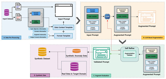
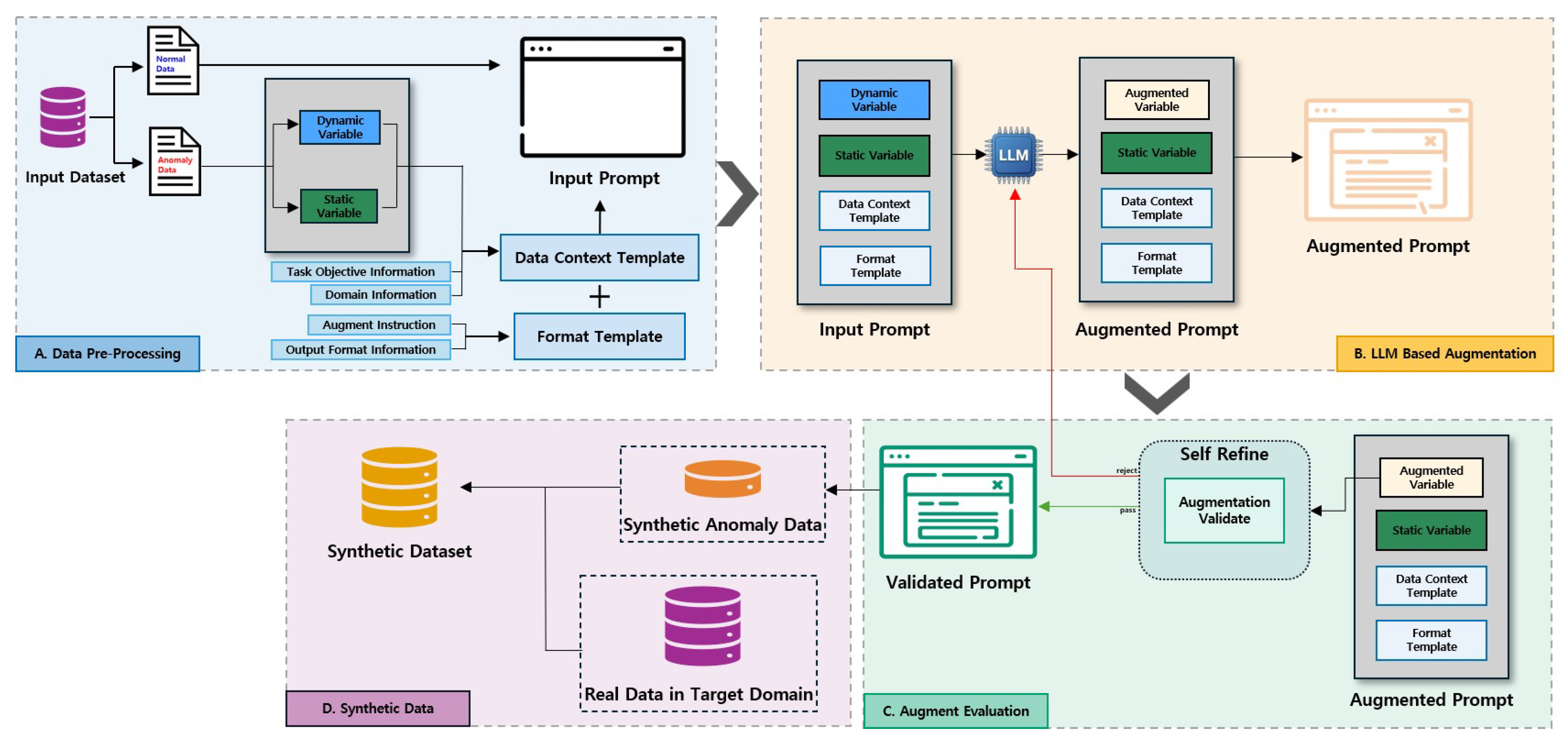


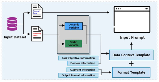
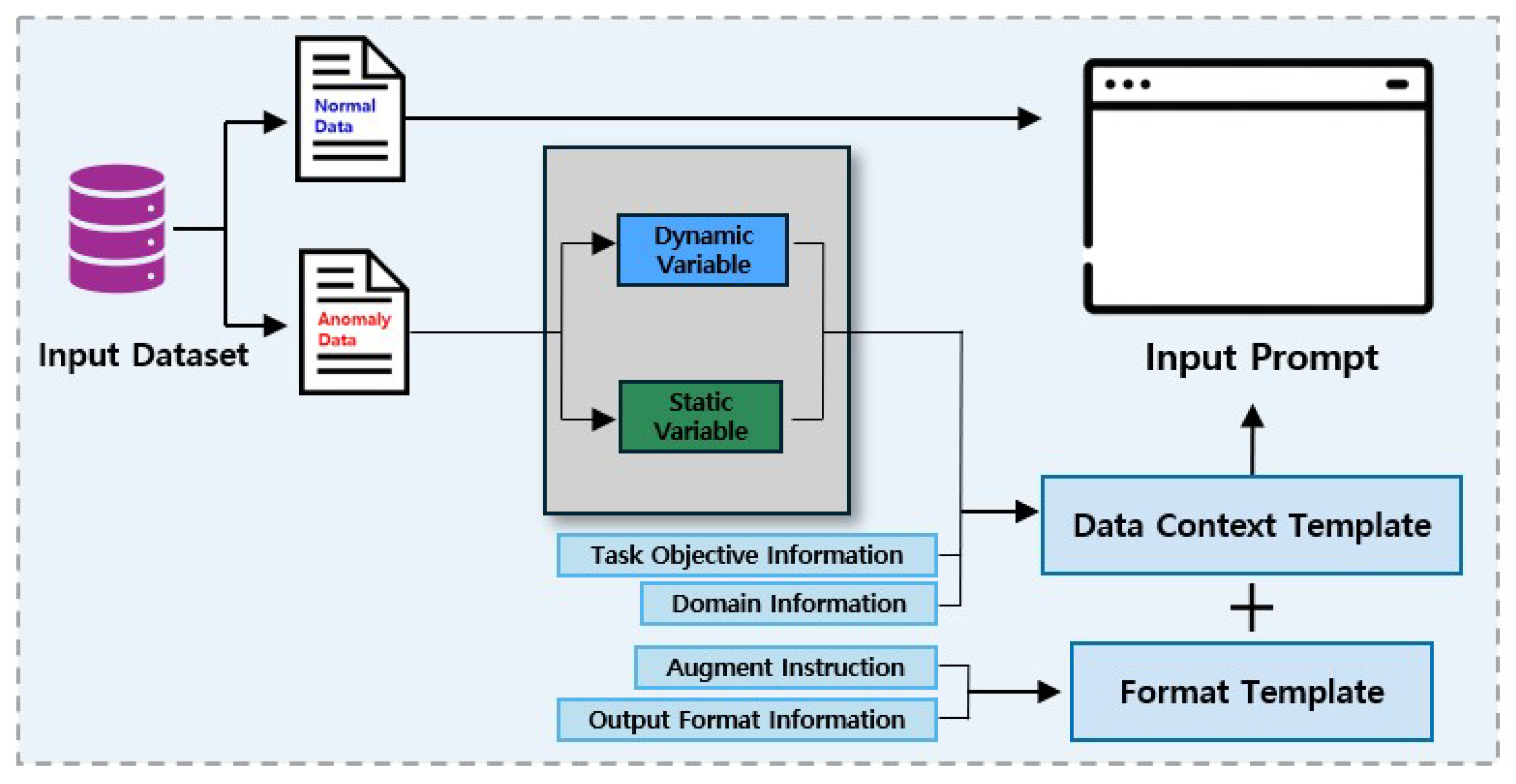
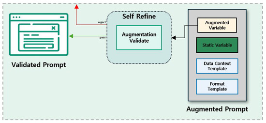
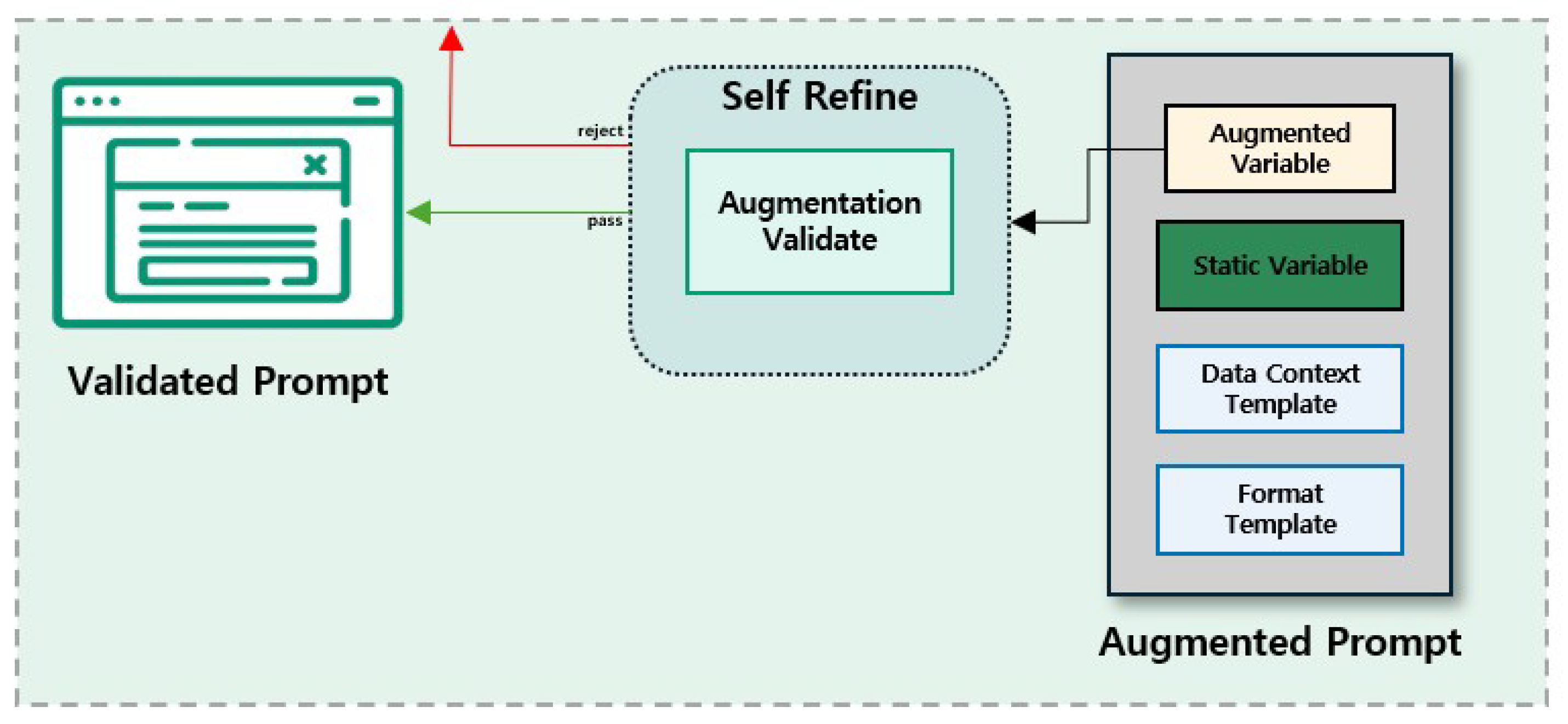
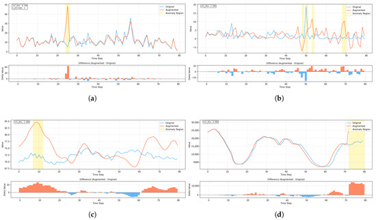
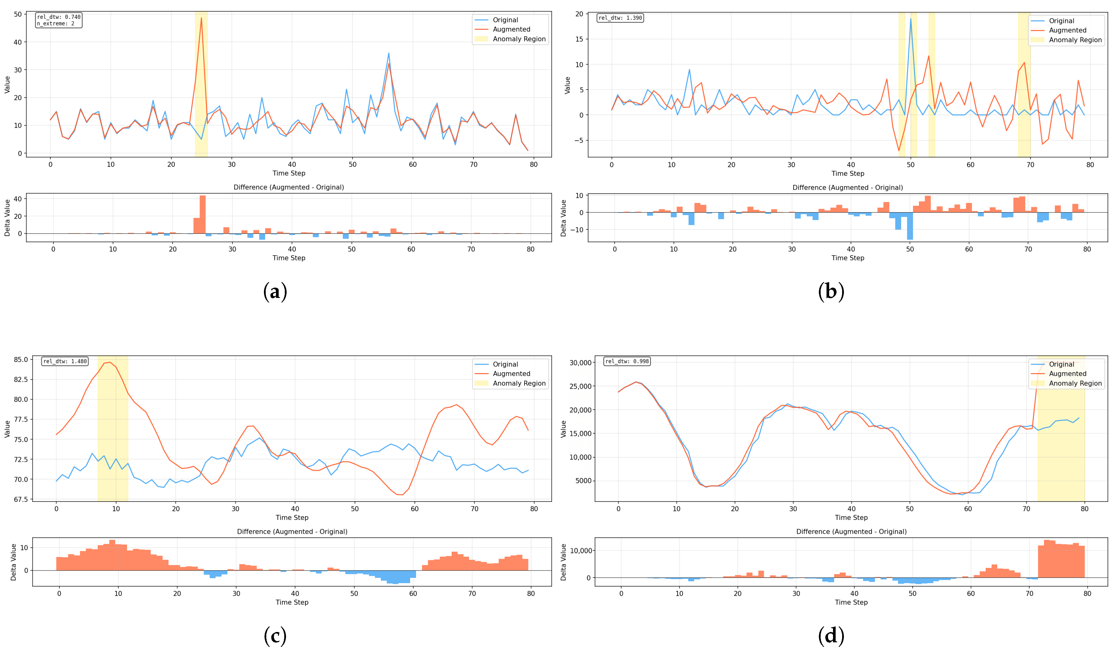
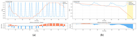
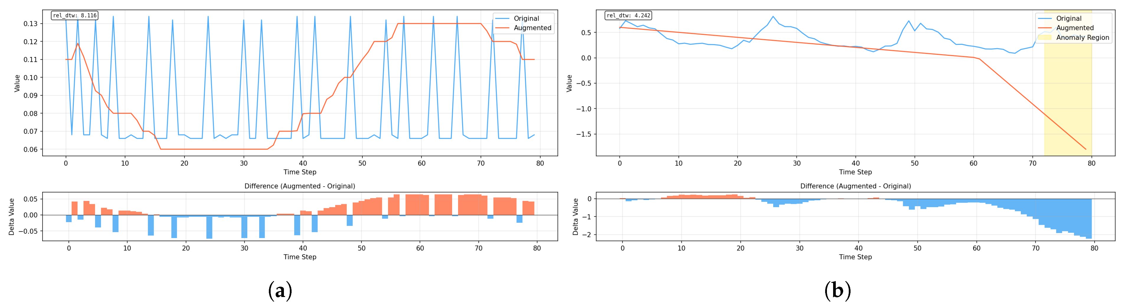
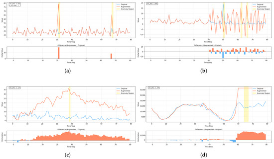
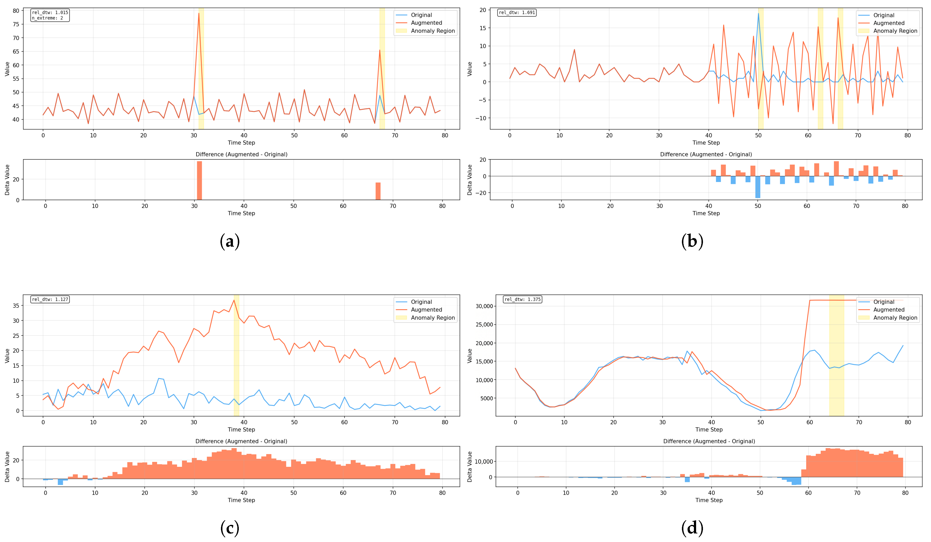
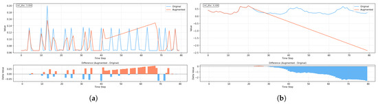
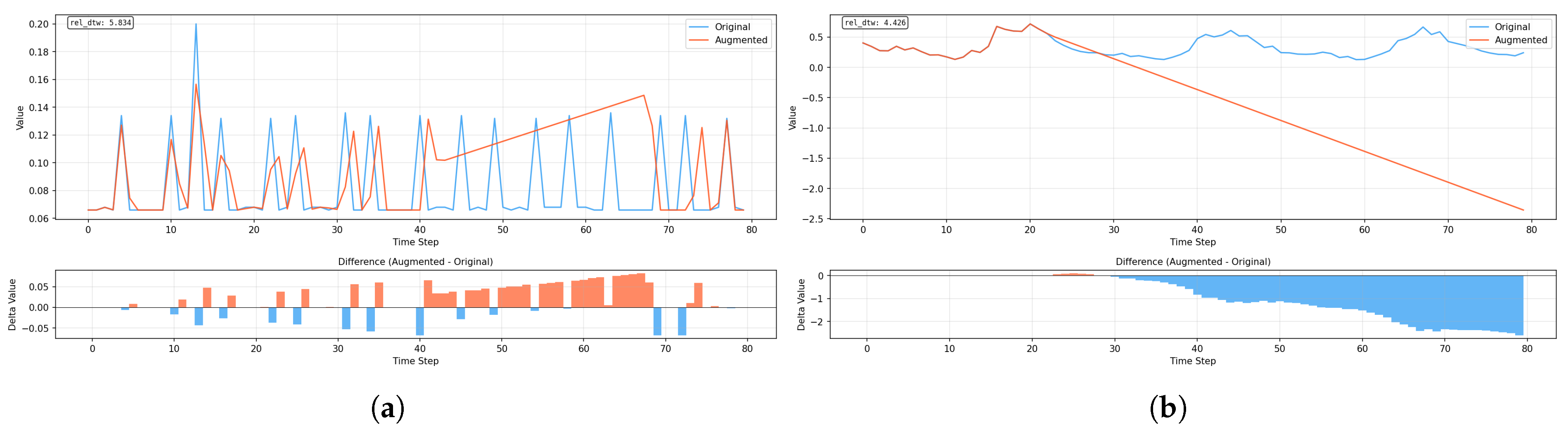

Disclaimer/Publisher’s Note: The statements, opinions and data contained in all publications are solely those of the individual author(s) and contributor(s) and not of MDPI and/or the editor(s). MDPI and/or the editor(s) disclaim responsibility for any injury to people or property resulting from any ideas, methods, instructions or products referred to in the content. |
© 2026 by the authors. Licensee MDPI, Basel, Switzerland. This article is an open access article distributed under the terms and conditions of the Creative Commons Attribution (CC BY) license.