


Abstract
Galloping of iced transmission lines under complex microclimates poses a severe threat to power grid security, whereas traditional full-span de-icing strategies suffer from excessive energy redundancy and limited spatial precision. To address the spatial uncertainty of actual ice accretion, a three-dimensional nonlinear aeroelastic finite element model is established by considering geometric nonlinearity and eccentric ice-induced added stiffness. A state-space Monte Carlo framework is then used to evaluate the galloping probability under different wind speed regimes and spatially non-uniform ice distributions. The results reveal a distinct non-monotonic instability characteristic: the galloping probability decreases to 33.0% at 8.0 m/s, forming a clear probability trough and indicating an aerodynamic self-stabilization effect associated with the shift in the baseline effective angle of attack. To map spatial ice heterogeneity to global dynamic instability, a galloping sensitivity index (GSI) based on the Spearman rank correlation coefficient is proposed to identify the dominant sensitive sections responsible for inducing galloping-prone responses. Based on this index, a GSI-guided targeted ultrasonic de-icing decision strategy is constructed. Under the assumption of identical rated power for each section, the proposed strategy activates only 40% of the physical sections and reduces the number of activated sections, as well as the associated operational energy demand, by 60% compared with the full-span de-icing strategy. This framework provides a quantitative basis for linking stochastic ice distribution, galloping probability evaluation, and energy-efficient targeted de-icing decisions.
1. Introduction
Overhead transmission lines, as typical long-span super-flexible structures, exhibit high susceptibility to ice accretion in cold micro-meteorological environments [1]. Under crosswinds, the alteration of aerodynamic characteristics of the conductor cross-section can trigger low-frequency, large-amplitude self-excited vibrations known as conductor galloping. Mechanically, galloping of iced conductors is a complex fluid–structure interaction (FSI) phenomenon driven by aeroelastic instability [2,3]. This violent dynamic response not only causes the structure to continuously extract energy from the wind field and evolve into limit cycle oscillations but also potentially leads to fatigue breaking of conductors, phase-to-phase flashovers, and even catastrophic tower-collapses or line-breakages, posing a severe challenge to the safety and reliability of power grid operation [4,5].
To effectively mitigate galloping disasters, the academic and engineering communities have developed various anti-galloping measures, covering passive vibration reduction devices represented by anti-galloping pendulums and aerodynamic dampers, as well as active de-icing control technologies that have attracted extensive research interest in recent years [6,7,8]. Passive measures are generally simple and suitable for long-term installation, but their effectiveness is often condition-dependent when ice morphology, wind direction, and modal coupling vary [9,10,11,12,13]. Active methods, such as thermal ice melting, mechanical ice removal, and ultrasonic de-icing, can directly reduce ice-induced aerodynamic excitation, but conventional operations usually lack spatial targeting capability [9,10,14]. Among active control methods, ultrasonic de-icing has become a research hotspot because it can promote ice–conductor interfacial fracture through localized, controllable, and energy-efficient mechanical vibration excitation [15,16]. However, existing de-icing operations mostly adopt a conservative “full-span clearing” strategy. This indiscriminate intervention strategy not only causes significant energy redundancy when dealing with modern long-span transmission networks but also suffers from limited operational efficiency, hindering the realization of targeted and energy-optimal disaster governance [17,18].
It should be emphasized that under the combined influence of local micro-topography, temperature gradients, and the spatial coherence of turbulent wind fields, the ice distribution on the conductor surface within actual spans exhibits significant spatial non-uniformity and randomness [19,20]. However, existing deterministic dynamic models generally adopt the simplified assumption of “uniform ice thickness across the span,” which directly masks the sensitivity of the system to local eccentric excitation. This deterministic analysis paradigm often fails to effectively capture the internal resonance and frequency coupling induced by the evolution of local asymmetric ice, limiting the accurate prediction of the critical boundary for aeroelastic instability [21,22]. Therefore, shifting from deterministic analysis to probabilistic assessment considering the uncertainty of spatial ice distribution is of great scientific significance and engineering value for deeply exploring the galloping instability mechanism and formulating efficient targeted intervention strategies.
Compared with previous studies, the main knowledge gap lies in the lack of a unified framework that connects stochastic spatial ice distribution, nonlinear galloping probability evaluation, and section-level targeted de-icing decision-making. Existing deterministic models usually simplify the ice distribution as uniform along the span, which makes it difficult to identify the local ice-eccentricity perturbations that dominate the global instability process. In addition, conventional de-icing strategies are mostly based on full-span clearing, and the quantitative relationship between local ice-distribution sensitivity and targeted intervention priority remains insufficiently explored.
To address these gaps, the main contributions of this study are summarized as follows:
- (1)
- a three-dimensional nonlinear aeroelastic numerical model is established to describe the coupled vertical, crosswind, and torsional galloping response of iced conductors with geometric nonlinearity and ice-eccentricity-induced stiffness effects;
- (2)
- a Monte Carlo-based stochastic simulation framework is developed to evaluate the galloping probability under spatially non-uniform ice distributions and different wind speeds;
- (3)
- a Galloping Sensitivity Index (GSI) is proposed based on Spearman rank correlation to quantify the contribution of each physical section to the global instability state;
- (4)
- a GSI-guided targeted ultrasonic de-icing decision strategy is constructed to identify dominant sensitive sections and reduce unnecessary full-span intervention.
2. Nonlinear Aeroelastic Coupled Numerical Model Considering Eccentric Added Stiffness
To accurately reveal the aeroelastic instability trajectory of iced conductors under complex wind fields, a three-dimensional nonlinear FSI numerical model is developed based on the three-node quadratic curved beam finite element theory. The model incorporates geometric nonlinearity induced by large-displacement sag and eccentric ice effects within the structural domain, while integrating a spatially coherent turbulent wind model and nonlinear aerodynamic polynomials within the fluid domain. The governing equations are solved in the time domain using an incremental integration scheme.
2.1. Finite Element Discretization and Dynamic Governing Equations of the Conductor
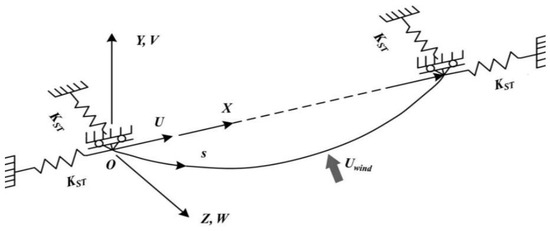
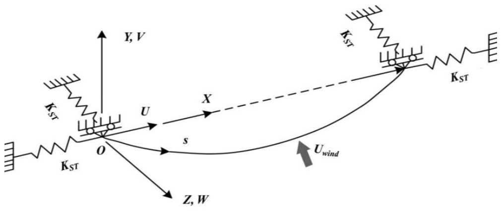
As a typical multi-scale flexible cable structure, transmission conductors exhibit pronounced multi-degree-of-freedom (DOF) coupling characteristics under asymmetric ice accretion and wind load excitation. To improve the interpolation accuracy of the displacement field and better represent the curved configuration of the conductor, a three-node quadratic isoparametric curved beam element is employed for spatial discretization [23,24,25], as illustrated in Figure 1. Each element consists of two end nodes and one mid-span node, with each node assigned four independent DOFs:
where represents the axial displacement along the conductor; is the vertical displacement; is the crosswind displacement; and is the torsional rotation angle around the principal axis.
Figure 1.
Schematic diagram of the transmission conductor.
The displacement field within the element is interpolated using quadratic Lagrange shape functions (where ). The global nonlinear dynamic governing equation in the time domain is expressed as:
where , , and are the global mass, damping, and stiffness matrices, respectively; is the aerodynamic force vector explicitly dependent on the instantaneous state of the structure. The damping matrix is formulated using the Rayleigh damping model and calibrated based on the first and third natural circular frequencies of the system. For each Monte Carlo realization, modal analysis is first performed using the corresponding mass and stiffness matrices, and the Rayleigh damping coefficients are then recalibrated according to the selected modal frequencies. The Rayleigh damping matrix is expressed as . For the baseline full-ice case, the target damping ratios of the two calibration modes are set as ζ1 = ζ3 = 0.08%. The first and third natural circular frequencies used for calibration are ω1 = 2.96 rad/s, ω3 = 3.36 rad/s, corresponding to f1 = 0.47 Hz, f3 = 0.53 Hz. The resulting Rayleigh damping coefficients are αR = 2.52 × 10⁻³, βR = 2.53 × 10⁻⁴.
2.2. Structural Mass and Stiffness Matrices
To achieve high-fidelity mapping of the conductor’s physical parameters, the element matrices are derived through symbolic integration.
(1) Mass matrix decomposition: The element mass matrix is decomposed into an independent superposition of translational mass and torsional mass moment of inertia, eliminating redundant centrifugal coupling terms to enhance computational efficiency:
where is the equivalent mass per unit length of the iced conductor; is the mass moment of inertia per unit length; is the element length; and and are the shape function matrices corresponding to translational and torsional DOFs, respectively.
(2) Three-dimensional reconstruction of the stiffness matrix: The element stiffness matrix comprehensively accounts for material constitution, initial tension, and ice eccentric effects, formulated as the sum of three components: .
Linear elastic stiffness : Governed by the material’s axial stiffness , bending stiffness , and torsional stiffness .
Initial tension geometric stiffness : For long-span flexible cables, out-of-plane stiffness is primarily maintained by axial tension. Based on the initial static horizontal tension , the stress stiffening matrix is constructed by extracting the first derivatives of the vertical and crosswind shape functions ():
Following the three-node cable-element formulation of Desai et al., the initial horizontal tension is introduced through the geometric stiffness matrix associated with the vertical and crosswind deformation gradients [17]. In the present D-shaped iced conductor model, no additional independent tension-induced pure torsional stiffness term is introduced; the torsional resistance is governed by , while the torsional softening and torsional–vertical coupling are mainly represented by the eccentric ice-induced stiffness and the aerodynamic moment.
Eccentric ice-induced added stiffness : Asymmetric ice accretion shifts the mass center from the centroid. Under the gravitational field , the mass area moment generates a restoring moment that varies with the torsional angle, manifesting as a significant negative stiffness effect (stress softening):
This negative stiffness term directly weakens the torsional resistance of the conductor, serving as the mechanical origin of torsional-vertical frequency proximity and internal resonance [26].
2.3. Spatial Coherent Wind Field and Nonlinear Aerodynamic Force Calculation
(1) Spatial coherent pulsating wind field simulation
Due to the vast span of transmission lines, spatial wind field coherence must be considered [27,28]. This study employs the Kaimal double-sided power spectrum to represent turbulence energy distribution in the frequency domain, combined with the Davenport coherence function to construct the cross-power spectral density (CPSD) matrix. By performing Cholesky decomposition on the CPSD matrix and applying random phases, a spatiotemporally correlated wind speed matrix covering all discrete nodes is generated via inverse fast Fourier transform (IFFT) [29,30].
(2) Nonlinear aerodynamic force mapping
Based on the quasi-steady aerodynamic assumption, the instantaneous effective angle of attack is determined by the mean static wind angle , nodal vertical vibration velocity , torsional angular velocity , and the instantaneous wind speed:
where R is the conductor radius (m), is the nodal vertical vibration velocity (m/s), is the torsional angular velocity (rad/s), Uinst is the instantaneous wind speed (m/s), and αt and α0 are expressed in radians.
To avoid repeated coordinate transformations during time integration, the aerodynamic coefficients Cy, Cz, and Cθ are expressed in the structural coordinate system corresponding to the vertical, crosswind, and torsional force components. Polynomial fitting is commonly used to describe the nonlinear variation in aerodynamic coefficients over a wide range of angles of attack [31,32,33]. In this study, the polynomial aerodynamic coefficient functions are adopted from the curve-fitted wind-tunnel data of the D-shaped iced conductor reported by Desai et al. [17]:
The transient aerodynamic force components per unit length () are updated accordingly as and distributed to the nodes via integration weights. In the subsequent stochastic simulations, these coefficient functions are used as the baseline aerodynamic input for all physical sections, while the spatial uncertainty of icing is introduced through section-level mass, inertia, and eccentricity-related parameters, as described in Section 3.1.
2.4. Dynamic Tension Compensation Based on Static Catenary Reference
Large-amplitude galloping triggers significant geometric deformation, leading to dynamic fluctuations in axial tension. Assuming constant tension would result in severe distortion of the displacement response. Therefore, a geometric nonlinear tension correction mechanism based on a “static catenary reference” has been developed.
First, the initial static coordinates of the conductor under self-weight are reconstructed based on parabolic theory to calculate the precise static initial arc length . At each dynamic time step t, nodal absolute displacements are extracted to update spatial coordinates, and the current deformed dynamic total arc length is cumulatively calculated via difference norms:
The global axial dynamic tension is compensated in a closed loop based on real-time physical strain:
This mechanism ensures that tension reduction during upward movement and tension surge during downward movement strictly adhere to physical laws. This not only prevents numerical divergence during the evolution of large-amplitude limit cycles but also provides the essential algorithmic foundation for high-precision galloping probability assessment and the rigorous solution of anti-galloping safety displacements [34,35].
2.5. Time-Domain Incremental Solution of Governing Equations
The governing equations are solved in the time domain using the average-acceleration Newmark-β integration algorithm with β = 0.25 and γ = 0.5. For each Monte Carlo realization, the global mass, stiffness, and damping matrices are assembled according to the corresponding spatial ice distribution. The effective dynamic stiffness matrix is constructed before the time-integration loop as:
where .
To improve computational efficiency during large-scale time-history simulations, is factorized by LDL decomposition and reused within the time-stepping process.
At each time step, the instantaneous aerodynamic force vector is updated based on the current nodal motion state and the simulated wind velocity. The effective angle of attack is evaluated according to Equation (6), and the corresponding aerodynamic force and moment are obtained using the polynomial aerodynamic coefficient functions in Equations (7)–(9). The aerodynamic loads are then transformed into equivalent nodal loads and incorporated into the Newmark effective load vector. Subsequently, the displacement increment is solved using the pre-factorized effective stiffness matrix, and the acceleration, velocity, and displacement vectors are updated sequentially. This incremental procedure enables efficient tracking of the aeroelastic response under spatially uncertain icing conditions [36].
3. Galloping Probability Evaluation and Non-Monotonic Instability Mechanism Under Uncertain Ice Distribution
In this section, spatial heterogeneity of the ice layer is coupled into the three-dimensional aeroelastic model by introducing dimensionless spatial random vectors. Leveraging large-scale Monte Carlo time-history simulations, the aeroelastic instability boundaries of iced conductors across multiple wind speed regimes are quantitatively evaluated. Furthermore, the underlying modulation mechanisms of spatial uncertainty on system energy evolution and bifurcation topology are analyzed in depth.
3.1. Stochastic Modeling of Non-Uniform Ice Distribution
In actual micro-meteorological environments, the growth process of ice along the span is influenced by the coupling of local flow disturbances and temperature gradients, exhibiting high spatial randomness. To incorporate the spatial variability of continuous ice layers into deterministic dynamic equations, this model reconstructs the physical attributes of each discrete element using parameterized random vectors.
To focus on the influence of local mass-eccentricity perturbations on the global galloping response, the ice mass variation coefficients of the discrete elements are described using an independent uniform sampling scheme in the present probabilistic framework. This treatment provides a non-informative representation of local ice-mass fluctuation within a prescribed range and avoids introducing an assumed correlation length without site-specific icing observations. Accordingly, the ice mass variation coefficient for the e-th element is defined as:
This interval defines a local ice mass fluctuation between 50% and 150% of the baseline full-ice state. It should be noted that actual ice accretion along transmission lines may exhibit spatial correlation due to continuous meteorological gradients. Therefore, the present assumption is mainly used for local sensitivity screening and probabilistic framework demonstration, while spatially correlated random fields will be incorporated in future extensions when reliable correlation lengths or field monitoring data are available.
Controlled by this variation coefficient, the equivalent translational mass , mass moment of inertia , and the mass area moment representing the eccentric effect are all transformed into coordinate-dependent random variables:
Through the assembly of the Boolean topology matrix, these local random parameters are mapped onto the global mass matrix and the eccentric added stiffness matrix . This stochastic matrix reconstruction not only alters the natural frequency spectrum of the system but also necessitates dynamic calibration of the Rayleigh damping matrix during each sampling, thereby high-fidelity restoring the spatial drift of aerodynamic energy dissipation characteristics caused by non-uniform icing.
3.2. Evaluation Framework for Aeroelastic Instability
Galloping is essentially a limit cycle bifurcation (Hopf Bifurcation) triggered when the unsteady aerodynamic negative damping energy extracted from the constant wind field exceeds the structural mechanical dissipation. Due to the low-frequency response characteristics of long-span conductors, short-term analysis can easily misinterpret forced buffeting extrema as self-excited galloping amplitudes. Therefore, this study establishes a rigorous instability criterion based on the asymptotic functional of the final state.
The integration time is set to t = 18,000 s to ensure that transient free vibrations are fully dissipated. The time-domain integration starts from the reference static configuration of the conductor, with zero incremental displacement and zero initial velocity; no additional artificial displacement or velocity perturbation is imposed. A Boolean indicator function is introduced to extract the instantaneous absolute value of the vertical displacement at the mid-span node in the final state. For the conductor model considered in this study, the design span length is L = 125.88 m. A peak-displacement criterion is adopted because the primary engineering risks of conductor galloping, such as insufficient electrical clearance and phase-to-phase flashover, are directly governed by the maximum spatial excursion of the conductor. With Vthresh = 0.50 m as the engineering anti-galloping safety tolerance threshold for this medium-span conductor, the failure state of the k-th Monte Carlo sample is defined as:
Relying on the law of large numbers, the global failure probability of galloping at a given mean wind speed approximates the expected failure of the Monte Carlo samples
where NM is the total number of Monte Carlo simulations conducted for each wind speed regime. In this study, NMC = 100 samples are generated for each mean wind speed. Systematic sampling is conducted for wind speeds ranging from 6.0 m/s to 10.0 m/s to map the instability boundaries under the combined effects of wind dynamic pressure and uncertain ice distribution.
3.3. Non-Monotonic Evolution of Galloping Probability Across Wind Speeds
The global probability evolution curve reveals a highly significant non-monotonic dynamic characteristic. While traditional deterministic theories often assume that wind-induced response monotonically worsens with increasing wind speed, the comprehensive Monte Carlo evaluation results challenge this conventional understanding.
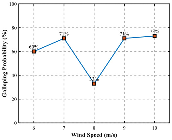
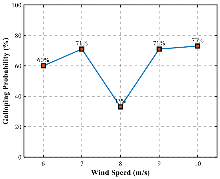
As shown in Figure 2, at sub-critical wind speeds of 6.0 m/s and 7.0 m/s, asymmetric icing easily crosses the negative damping threshold, resulting in galloping probabilities as high as 60.0% and 71.0%, respectively. However, as the wind speed rises to 8.0 m/s, the galloping probability undergoes a sharp decline, plummeting to 33.0% and forming a prominent “probability trough.” As the wind speed further increases to 9.0 m/s and 10.0 m/s, the powerful dynamic pressure of the flow field reclaims dominance in energy injection, and the galloping probability rapidly rebounds and stabilizes at a high level (71.0% and 73.0%).
Figure 2.
Galloping occurrence probability of non-uniform iced conductors at different wind speeds.
3.4. Aerodynamic Stabilization Mechanism: Shift in the Baseline Angle of Attack
The “probability trough” occurring at 8.0 m/s profoundly indicates that aeroelastic instability of iced conductors is not solely governed by the absolute magnitude of wind dynamic pressure. Its physical root lies in the shift in the fluid–structure coupling baseline induced by high wind pressure.
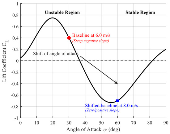
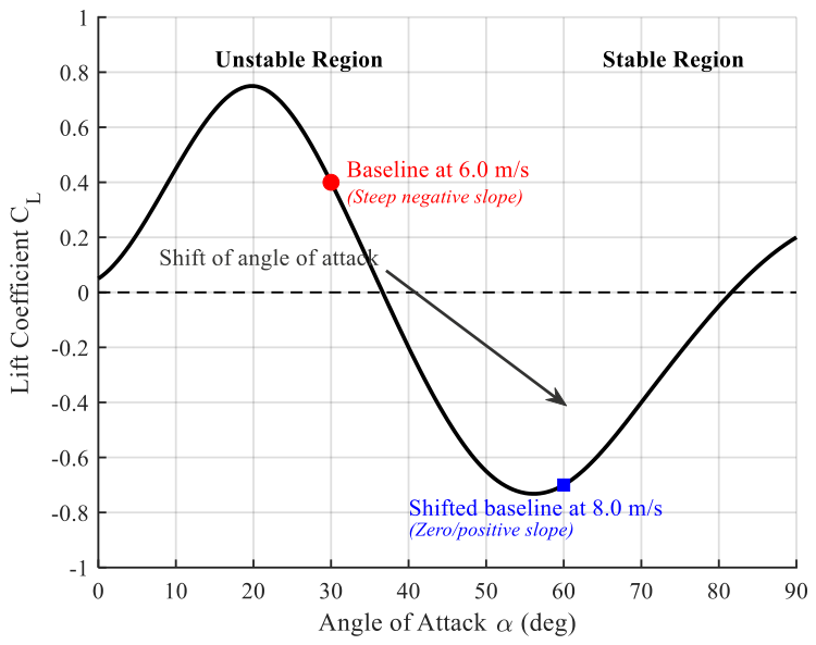
Increasing wind speed not only amplifies the alternating aerodynamic lift but also significantly increases the initial static wind drag load borne by the system. Under strong crosswinds, the conductor undergoes substantial static blow-out and additional torsion, leading to a shift in the mean baseline equilibrium position of the cross-section. As illustrated in Figure 3, under the specific high wind pressure at 8.0 m/s, the baseline effective angle of attack of the system is precisely shifted into the non-negative damping region of the aerodynamic lift coefficient () curve (i.e., the region where the slope is positive or gently slightly negative).
Figure 3.
Schematic of aerodynamic stabilization induced by baseline angle of attack shift.
This shift may reduce the aerodynamic negative-damping contribution associated with the Den Hartog-type galloping mechanism, thereby limiting the continuous accumulation of aerodynamic energy for part of the stochastic samples. In this state, despite the immense total kinetic energy of the wind field, the incremental work injected into the structure by the flow field cannot overcome the single-cycle mechanical dissipation of the structural Rayleigh damping. Consequently, at 8.0 m/s, approximately 67% of the spatially non-uniform ice samples are forced to converge below the safety threshold, manifesting as a macroscopic aerodynamic self-stabilization effect.
3.5. Energy Divergence and Local Modulation in State Space
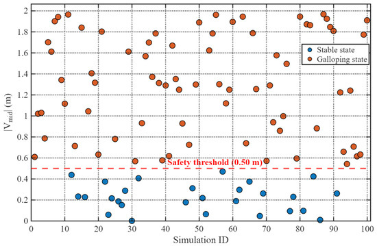
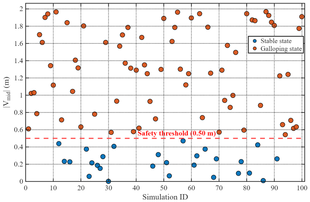
To gain insight into the local modulation effect of non-uniform icing on the limit-cycle energy of the system at high-risk wind speeds, the peak vertical displacements of each sample at the final state are extracted to plot the state-space scatter distribution, as shown in Figure 4.
Figure 4.
Scatter distribution of the final absolute mid-span displacement under uncertain spatial ice distributions (U = 10.0 m/s).
The divergence of the scatter groups visually characterizes the perturbative effect of spatial heterogeneity on global instability. At high-risk wind speeds of 10.0 m/s, even when the total ice mass across the span is similar, the steady-state responses (red vs. blue dots) of different samples exhibit immense variance. Amplitudes in some unstable cases approach 2.0 m, whereas in safe cases, they are suppressed below 0.2 m. This provides compelling evidence that the decisive factor in large-amplitude galloping is not the total ice volume, but the specific spatial heterogeneous distribution patterns. Certain local asymmetric ice peaks act as excitation sources, profoundly weakening local torsional stiffness through “stress softening” and forcing the natural frequencies of torsional and vertical DOFs into internal proximity. Once this global frequency coupling is triggered, wind energy is injected into the system at a geometric rate. This finding provides the theoretical foundation for the subsequent “targeted de-icing strategy” aimed at breaking frequency coupling through local perturbation.
4. Optimal Targeted De-Icing Control Strategy Based on Spatial Sensitivity Analysis
In the extreme high-risk wind speed regime, the overall system has surpassed the Hopf bifurcation point. The traditional full-span ice clearing strategy, aimed at restoring geometric consistency across the entire span, is confronted with immense operational energy consumption and energy redundancy. To achieve the control objective of breaking the global aeroelastic instability with minimal local physical perturbations, this section proposes an energy-optimal targeted ultrasonic de-icing strategy based on the sensitivity of the spatial ice distribution.
4.1. Mapping Mechanism Between Spatial Heterogeneity and Aeroelastic Instability
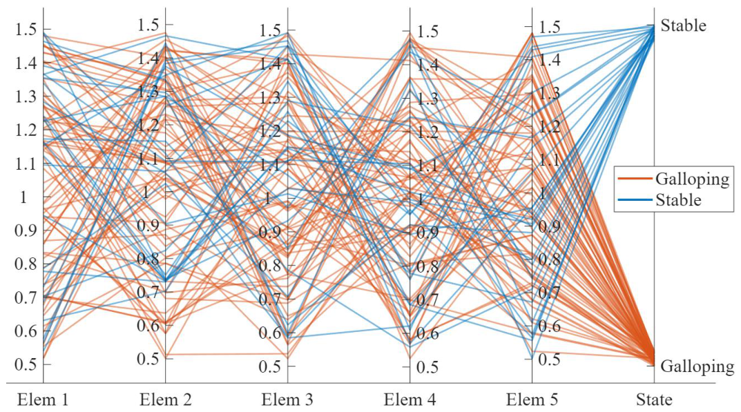
The results of the Monte Carlo time-history analysis indicate that under identical mean wind field excitations and equivalent total ice masses across the span, the ultimate dynamic responses of the system exhibit pronounced bifurcation characteristics (i.e., evolving into either large-amplitude limit cycles or micro-amplitude buffeting). This phenomenon fundamentally proves from a physical perspective that the critical parameter governing the instability boundary of iced conductors is not the extreme value of the total ice mass, but rather the nonlinear modulation of the overall energy evolution path of the system by the local spatial heterogeneous distribution. To quantify this modulation mechanism, the sequences of ice variation coefficients under the high-risk condition of U = 10.0 m/s are extracted and mapped onto the state space.
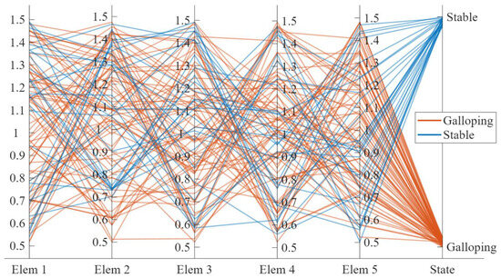
The state-space mapping diagram (Figure 5) reveals a significant numerical divergence between the safely converged samples and the unstable divergent samples at specific spatial elements. This demonstrates that specific combinations of local asymmetric ice accretion can alter the effective torsional stiffness of the cross-section, thereby triggering (or breaking) the internal resonance proximity condition between the torsional and vertical degrees of freedom.
Figure 5.
Mapping relationship between spatial distribution of non-uniform icing and galloping states at 10.0 m/s.
4.2. Mathematical Construction of the GSI
The structural “weak point” in a physical sense does not refer to the location with the maximum absolute ice thickness, but rather the critical local section that provides the maximum negative damping contribution to breaking the global frequency barrier of the system. To precisely identify this section, the Spearman rank correlation coefficient () is introduced to construct the dimensionless GSI.
The rank correlation coefficient of the i-th spatial discrete section is defined as the correlation measure between its ice variation coefficient and the final Boolean instability state of the system. The GSI of the i-th section is calculated as follows:
where is the total number of physical intervention sections along the span. This equation utilizes the absolute values of the correlation coefficients for global normalization, filtering out the directional differences in positive and negative correlations, and accurately mapping the sensitivity weights of local parameter perturbations on global instability.
The engineering diagnostic threshold is defined as
where denotes the mean sensitivity level under the assumption that all physical intervention sections contribute equally to galloping instability and λ is the engineering diagnostic multiplier. In this study, λ = 1.25 is adopted to identify sections whose sensitivity is at least 25% higher than the mean sensitivity level. This setting is intended to filter out sections with only average-level sensitivity while retaining the dominant sections that make a substantial contribution to galloping instability.
It should be noted that Nsec refers to the number of physical de-icing or intervention sections rather than the finite element mesh density used for structural dynamic analysis. When a finer finite element mesh is adopted, several finite elements can be grouped into one physical intervention section, and the section-level GSI can then be used for the activation decision.
When a spatial section satisfies , the algorithm identifies this section as the critical weak point inducing the current fluid–structure coupling resonance.
4.3. Mathematical Formulation and Intervention Mechanism for Targeted De-Icing
Based on the aforementioned GSI diagnostic criteria, the targeted de-icing strategy is formulated using a Boolean spatial intervention vector, with the structural anti-galloping safety limit and the total energy consumption of the ultrasonic de-icing system considered simultaneously. The corresponding mathematical formulation is expressed as:
where is the total energy consumption of the de-icing operation; is the Boolean spatial decision variable, where indicates initiating targeted intervention on the i-th section and indicates maintaining the original state; denotes the rated power consumption for executing a single ultrasonic intervention on section i; represents the extreme dynamic vertical displacement of the mid-span node after local intervention; and is the engineering anti-galloping safety tolerance threshold (set to 0.50 m in this study).
In the numerical implementation, the Boolean spatial intervention vector is determined from the section-level GSI diagnosis. Physical sections satisfying are assigned xi = 1, indicating that targeted de-icing intervention is activated in these sections, whereas the remaining sections are assigned xi = 0. The total energy demand is then evaluated according to the activated sections and their rated power Wi.
Frequency decoupling mechanism based on physical profile perturbation: The physical execution logic of this optimization model possesses significant novelty. During intervention execution (), the control system is not required to completely remove the ice in the target section. Instead, local ultrasonic excitation is utilized to disrupt the asymmetric aerodynamic profile of the ice body, thereby forcing its nonlinear aerodynamic coefficients to degrade and reconstruct towards a low-eccentricity baseline state. This localized physical perturbation weakens the dominant frequency coupling between torsional and vertical motions, thereby contributing to the suppression of divergent galloping responses.
4.4. Engineering Validation of the Targeted De-Icing Decision
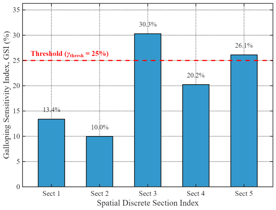
To intuitively validate the robustness of the aforementioned targeted de-icing decision, a numerical demonstration is conducted using the statistical samples at a wind speed of 10.0 m/s. For the targeted de-icing decision, the single span is divided into five physical intervention sections (Nsec = 5). The mean sensitivity level is therefore . With the engineering diagnostic multiplier λ = 1.25, the corresponding diagnostic threshold becomes .
(1) Parameter extraction and base calculation: Evaluated through the state space, the ρs values for the five physical intervention sections along the span are {−0.055, −0.041, −0.124, 0.083, 0.107}, respectively, based on NMC = 100 Monte Carlo samples at a wind speed of 10.0 m/s. The global sensitivity base is computed as .
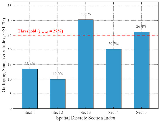
(2) Sensitivity diagnosis: Substituting these values into the GSI equation yields the sensitivity of each physical intervention section, with the results shown in Figure 6. Notably, the mid-span section 3 () and the end section 5 () exceed the diagnostic threshold of 25%.
Figure 6.
Sensitivity distribution of icing coefficients along the conductor span to the galloping probability.
The corresponding p-values and GSI values are summarized in Table 1. The p-values are reported to provide the statistical evidence level of the Spearman rank correlations, while the GSI values are used for section-level relative sensitivity diagnosis.
Table 1.
Spearman rank correlation coefficients, p-values, and GSI values of physical intervention sections.
(3) Threshold sensitivity analysis: To further examine whether the selected de-icing sections are sensitive to the engineering diagnostic multiplier, a threshold sensitivity analysis was conducted by varying λ from 1.00 to 1.50. The results are summarized in Table 2. When λ = 1.00, the diagnostic threshold is 20.0%, and sections 3–5 are selected. This setting is relatively loose because section 4 only slightly exceeds the mean sensitivity level. When λ varies from 1.10 to 1.30, the selected dominant sections remain sections 3 and 5, indicating that the diagnostic result is not highly sensitive to moderate variations in the multiplier. When λ ≥ 1.35, section 5 is excluded, suggesting that the threshold becomes relatively strict and may miss a physically relevant sensitive section. Therefore, λ = 1.25 is retained as a balanced engineering diagnostic multiplier between excessive intervention and missed detection of dominant sensitive sections.
Table 2.
Sensitivity of selected de-icing sections to the diagnostic multiplier.
(4) Decision output: Based on the GSI diagnosis and the threshold sensitivity analysis, the Boolean spatial intervention vector is obtained as indicating that sections 3 and 5 are selected as the dominant sensitive sections for targeted de-icing intervention.
This validation case demonstrates that the GSI-guided targeted de-icing decision framework can identify a limited number of dominant sensitive sections for priority intervention. Under the assumption of identical rated power for each section, activating sections 3 and 5 corresponds to intervening in only 40% of the physical sections. Compared with the traditional full-span de-icing strategy , the proposed strategy reduces the number of activated sections by 60%, while providing a targeted decision basis for suppressing galloping-prone spatial ice distributions.
4.5. Model Limitations and Applicability
This study focuses on the stochastic galloping probability evaluation and GSI-guided targeted de-icing decision of iced transmission conductors. Several limitations should be noted. First, the aerodynamic coefficient functions are adopted from the curve-fitted wind-tunnel data of a D-shaped iced conductor and are used as the baseline aerodynamic input. Therefore, the model is more suitable for galloping cases with similar ice profiles, while further calibration is required for other complex ice shapes. Second, the spatial uncertainty of icing is introduced through section-level mass, inertia, and eccentricity-related parameters, whereas the aerodynamic coefficient curves are not refitted for each local ice state. This simplification improves computational efficiency but may underestimate the aerodynamic influence of local ice-shape variation. Third, the present Monte Carlo framework uses a finite number of stochastic samples, and the GSI mainly provides a relative sensitivity ranking of physical sections. The diagnostic threshold sensitivity analysis in Table 2 is therefore used to examine the robustness of the selected de-icing sections. Finally, the proposed targeted de-icing decision is currently demonstrated at the numerical framework level. Further validation using scaled aeroelastic wind tunnel tests and field monitoring data will be necessary to improve the quantitative applicability of the model under realistic icing and wind conditions.
5. Conclusions
This study developed a stochastic aeroelastic simulation framework and a GSI-guided targeted de-icing decision strategy for iced transmission conductors considering uncertain spatial ice distributions. The main conclusions are summarized as follows:
- (1)
- A three-dimensional nonlinear aeroelastic model was established to describe the coupled vertical, crosswind, and torsional galloping response of iced conductors. By introducing spatially uncertain ice-distribution parameters into the Monte Carlo simulation framework, the proposed method provides a quantitative tool for evaluating galloping probability under non-uniform icing conditions.
- (2)
- The galloping probability exhibited a clear non-monotonic variation with wind speed. The calculated probability decreased from 71.0% at 7.0 m/s to 33.0% at 8.0 m/s, and then increased again to 71.0% at 9.0 m/s. This probability trough indicates that the galloping risk does not necessarily increase monotonically with wind speed when spatial ice uncertainty is considered. The shift in the baseline effective angle of attack may reduce the negative aerodynamic damping contribution and produce an aerodynamic self-stabilization effect under specific wind-speed conditions.
- (3)
- The proposed GSI identified the dominant sensitive sections for targeted de-icing. For the five physical intervention sections, sections 3 and 5 showed the highest GSI values of 30.2% and 26.1%, respectively, both exceeding the diagnostic threshold of 25%. Therefore, the targeted intervention vector was determined as indicating that only sections 3 and 5 need to be prioritized for de-icing intervention.
- (4)
- Compared with the traditional full-span de-icing strategy, the proposed GSI-guided strategy activates only 40% of the physical sections. Under the assumption of identical rated power for each section, this corresponds to a 60% reduction in the number of activated sections and the associated operational energy demand. The threshold sensitivity analysis further showed that the selected dominant sections remained unchanged when the diagnostic multiplier varied from 1.10 to 1.30, indicating the robustness of the targeted de-icing decision.
Author Contributions
Conceptualization, J.M. and Y.L.; methodology, J.M., J.W. and Y.L.; software, J.W.; validation, N.Z., G.Q., X.T. and J.W.; formal analysis, J.W. and Y.L.; investigation, N.Z., G.Q. and X.T.; resources, N.Z., G.Q. and X.T.; data curation, J.W.; writing—original draft preparation, J.W.; writing—review and editing, N.Z., J.M. and Y.L.; visualization, J.W.; supervision, J.M. and Y.L.; project administration, N.Z., J.M. and Y.L.; funding acquisition, J.M. and Y.L. All authors have read and agreed to the published version of the manuscript.
Funding
This research was funded by the Science and Technology Foundation of State Grid Corporation of China under grant number J2024149.
Institutional Review Board Statement
Not applicable.
Informed Consent Statement
Not applicable.
Data Availability Statement
The original contributions presented in the study are included in the article; further inquiries can be directed to the corresponding author.
Conflicts of Interest
Authors Nailong Zhang, Gang Qiu and Xiao Tan were employed by the company Electric Power Research Institute of State Grid Jiangsu Electric Power Co., Ltd. The remaining authors declare that the research was conducted in the absence of any commercial or financial relationships that could be construed as a potential conflict of interest.
Abbreviations
The following abbreviations are used in this manuscript:
| DOF | Degree of freedom |
| FSI | Fluid–structure interaction |
| GSI | Galloping sensitivity index |
| CPSD | Cross-power spectral density |
| IFFT | Inverse fast Fourier transform |
References
- Lee, J. Advanced Electrical and Electronics Engineering; Springer: Berlin, Germany, 2011. [Google Scholar]
- Hartog, J.P.D. Transmission Line Vibration Due to Sleet. Trans. Am. Inst. Electr. Eng. 1932, 51, 1074–1076. [Google Scholar] [CrossRef] [Scilit]
- Chen, X.; Wu, Y. Explicit Closed-Form Solutions of the Initiation Conditions for 3DOF Galloping or Flutter. J. Wind Eng. Ind. Aerodyn. 2021, 219, 104787. [Google Scholar] [CrossRef] [Scilit]
- Matsumiya, H.; Nishihara, T.; Yagi, T. Aerodynamic Modeling for Large-Amplitude Galloping of Four-Bundled Conductors. J. Fluids Struct. 2018, 82, 559–576. [Google Scholar] [CrossRef] [Scilit]
- Lilien, J.L.; Havard, D.G. Galloping Database on Single and Bundle Conductors Prediction of Maximum Amplitudes. IEEE Trans. Power Deliv. 2000, 15, 670–674. [Google Scholar] [CrossRef] [Scilit]
- Luongo, A.; Zulli, D.; Piccardo, G. On the Effect of Twist Angle on Nonlinear Galloping of Suspended Cables. Comput. Struct. 2009, 87, 1003–1014. [Google Scholar] [CrossRef] [Scilit]
- Laforte, J.L.; Allaire, M.A.; Laflamme, J. State-of-the-Art on Power Line de-Icing. Atmos. Res. 1998, 46, 143–158. [Google Scholar] [CrossRef] [Scilit]
- Parent, O.; Ilinca, A. Anti-Icing and de-Icing Techniques for Wind Turbines: Critical Review. Cold Reg. Sci. Technol. 2011, 65, 88–96. [Google Scholar] [CrossRef] [Scilit]
- Zhang, Z.; Zhang, H.; Yue, S.; Zeng, W. A Review of Icing and Anti-Icing Technology for Transmission Lines. Energies 2023, 16, 601. [Google Scholar] [CrossRef] [Scilit]
- Hu, J.; Liu, L.; Zhang, X.; Ju, Y. A Review of Transmission Line Icing Disasters: Mechanisms, Detection, and Prevention. Buildings 2025, 15, 3757. [Google Scholar] [CrossRef] [Scilit]
- Lou, W.; Chen, S.; Wen, Z.; Wang, L.; Wu, D. Effects of Ice Surface and Ice Shape on Aerodynamic Characteristics of Crescent-Shaped Iced Conductors. J. Aerosp. Eng. 2021, 34, 04021008. [Google Scholar] [CrossRef] [Scilit]
- Cui, F.; Zheng, K.; Liu, P.; Wang, H. Spatial Galloping Behavior of Iced Conductors under Multimodal Coupling. Sensors 2024, 24, 784. [Google Scholar] [CrossRef] [Scilit] [PubMed]
- Cui, F.; Zhang, S.; Huo, B.; Liu, X.; Zhou, A. Analysis of Stability and Modal Interaction for Multi-Modal Coupling Galloping of Iced Transmission Lines. Commun. Nonlinear Sci. Numer. Simul. 2021, 102, 105910. [Google Scholar] [CrossRef] [Scilit]
- Chen, Q.; Liu, T.; Wang, Z.; Miao, R. Research on Digital Twin Dynamic Modeling Method for Transmission Line Deicing System. Energies 2024, 17, 1424. [Google Scholar] [CrossRef] [Scilit]
- Shen, L.; Li, D.; Shang, Y.; Wang, J. Deicing Behavior and Residue Characteristic on Cold Surface Excited by Ultrasonic Vibration. Int. J. Refrig. 2023, 149, 168–180. [Google Scholar] [CrossRef] [Scilit]
- Jacob, S.; Pandey, S.; Moral, J.D.; Karimzadeh, A.; Gil-Rostra, J.; González-Elipe, A.R.; Borrás, A.; Winkler, A. Surface Acoustic Waves Equip Materials with Active De-Icing Functionality: Unraveled Glaze Ice De-Icing Mechanisms and Application to Centimeter-Scale Transparent Surfaces. Adv. Mater. Technol. 2023, 8, 2300263. [Google Scholar] [CrossRef] [Scilit]
- Guo, Z.; Zhang, T.; Jia, L.; Liu, R.; Duan, W. Intelligent Control and Optimization of Uninterrupted Power Serving De-Icing Technology for 110 kV Power Lines. Int. J. Low-Carbon Technol. 2024, 19, 1910–1918. [Google Scholar] [CrossRef] [Scilit]
- Qarahasanlou, A.N.; Barabady, J.; Barabadi, A. Atmospheric Ice Accretion Emergency Events Management: Power Distribution Networks. Results Eng. 2025, 27, 106162. [Google Scholar] [CrossRef] [Scilit]
- Fu, P.; Farzaneh, M.; Bouchard, G. Two-Dimensional Modelling of the Ice Accretion Process on Transmission Line Wires and Conductors. Cold Reg. Sci. Technol. 2006, 46, 132–146. [Google Scholar] [CrossRef] [Scilit]
- Xu, F.; Li, D.; Gao, P.; Zang, W.; Duan, Z.; Ou, J. Numerical Simulation of Two-Dimensional Transmission Line Icing and Analysis of Factors That Influence Icing. J. Fluids Struct. 2023, 118, 103858. [Google Scholar] [CrossRef] [Scilit]
- Lou, W.; Zhang, Y.; Xu, H.; Huang, M. Jump Height of an Iced Transmission Conductor Considering Joint Action of Ice-Shedding and Wind. Cold Reg. Sci. Technol. 2022, 199, 103576. [Google Scholar] [CrossRef] [Scilit]
- Lou, W.; Yang, L.; Huang, M.F.; Yang, X. Two-Parameter Bifurcation and Stability Analysis for Nonlinear Galloping of Iced Transmission Lines. J. Eng. Mech. 2014, 140, 04014081. [Google Scholar] [CrossRef] [Scilit]
- Rega, G. Nonlinear Vibrations of Suspended Cables—Part I: Modeling and Analysis. Appl. Mech. Rev. 2005, 57, 443–478. [Google Scholar] [CrossRef] [Scilit]
- Jayaraman, H.B.; Knudson, W.C. A Curved Element for the Analysis of Cable Structures. Comput. Struct. 1981, 14, 325–333. [Google Scholar] [CrossRef] [Scilit]
- Desai, Y.M.; Yu, P.; Popplewell, N.; Shah, A.H. Finite Element Modelling of Transmission Line Galloping. Comput. Struct. 1995, 57, 407–420. [Google Scholar] [CrossRef] [Scilit]
- Gao, M.; Chen, Z.; Su, J.; Su, N.; Liu, C.; Zhang, J.; Chen, H. Experimental Study on the Galloping Characteristics of Single Ice-Coated Transmission Lines under Oblique Flows. Sci. Rep. 2023, 13, 5172. [Google Scholar] [CrossRef] [Scilit] [PubMed]
- Deodatis, G. Simulation of Ergodic Multivariate Stochastic Processes. J. Eng. Mech. 1996, 122, 778–787. [Google Scholar] [CrossRef] [Scilit]
- Li, J.-X.; Zhang, C.; Fu, X. Wind-Induced Response Analysis of the Transmission Tower-Line System Considering the Joint Effect. Int. J. Struct. Stab. Dyn. 2024, 24, 2450252. [Google Scholar] [CrossRef] [Scilit]
- Xu, Z.; Wang, H.; Zhao, K.; Zhou, R.; Lin, Y. Super-Resolution Reconstruction of Simulated Stochastic Wind Fields Using Ensemble Conditional Diffusion Model. J. Wind Eng. Ind. Aerodyn. 2025, 267, 106249. [Google Scholar] [CrossRef] [Scilit]
- Lin, Y.; Wang, H.; Xu, Z.; Zhao, K. Canonical Polyadic Decomposition Enhanced Stochastic Wave-Based Spectral Representation Method for the Simulation of Nonstationary Turbulent Wind Fields. Mech. Syst. Signal Process. 2025, 232, 112740. [Google Scholar] [CrossRef] [Scilit]
- Parkinson, G.V.; Brooks, N.P.H. On the Aeroelastic Instability of Bluff Cylinders. J. Appl. Mech. 1961, 28, 252–258. [Google Scholar] [CrossRef] [Scilit]
- Wan, Z.; Zhang, D.; Li, Z.; Mo, S.; Zhang, Y. A Wind Tunnel Study on the Aerodynamic Characteristics of Ice-Accreted Twin Bundled Conductors. Int. J. Struct. Stab. Dyn. 2022, 22, 2250038. [Google Scholar] [CrossRef] [Scilit]
- Yang, A.; Duan, F.; Song, Y.; Liu, Z.; Liu, Y. Aerodynamic Characteristics and Galloping Response of Ice-Covered Additional Conductors in the Overhead Contact Line. Int. J. Struct. Stab. Dyn. 2025, 2650387. [Google Scholar] [CrossRef] [Scilit]
- Irvine, H.M.; Caughey, T.K. The Linear Theory of Free Vibrations of a Suspended Cable. Proc. R. Soc. Lond. Math. Phys. Sci. 1974, 341, 299–315. [Google Scholar] [CrossRef] [Scilit]
- Luongo, A.; Piccardo, G. Non-linear galloping of sagged cables in 1:2 internal resonance. J. Sound Vib. 1998, 214, 915–940. [Google Scholar] [CrossRef] [Scilit]
- Newmark, N.M. A Method of Computation for Structural Dynamics. J. Eng. Mech. Div. 1959, 85, 67–94. [Google Scholar] [CrossRef] [Scilit]

Disclaimer/Publisher’s Note: The statements, opinions and data contained in all publications are solely those of the individual author(s) and contributor(s) and not of MDPI and/or the editor(s). MDPI and/or the editor(s) disclaim responsibility for any injury to people or property resulting from any ideas, methods, instructions or products referred to in the content. |
© 2026 by the authors. Licensee MDPI, Basel, Switzerland. This article is an open access article distributed under the terms and conditions of the Creative Commons Attribution (CC BY) license.