Design and Experimental Study of a Cable-Driven Hexapod Soft Robot

Abstract

Line-driven soft robots possess inherent advantages in terms of cushioning and terrain adaptability, but the controllable deformation design of line-driven structures and its coordination mechanism with the overall robot motion remain insufficiently studied. To fill this gap, this paper designs a line-driven hexapod soft robot that achieves directional bending of flexible legs through unilateral line traction, combined with triangular gait co-motion and ROS-based multi-sensor perception. Integrating leg deformation as part of the motion mechanism enables the robot to achieve straight-line and turning movements while maintaining structural compliance. This paper establishes the mapping relationship between the leg actuation space, configuration space, and task space, constructs a kinematic model, and uses the finite element method to analyze leg deformation and stress distribution. Based on this, a robot prototype is built, and a ROS-based distributed control and perception system is constructed, utilizing LiDAR, camera, and attitude sensor data to achieve SLAM and state monitoring. Experimental results show that the robot can achieve continuous motion with an average speed of 15.32 mm/s and a turning angle of 4.75° in a single gait cycle. The feasibility of line-driven structure control based on unilateral traction was verified, and a reference was provided for the design of soft robots oriented towards environmental perception.

1. Introduction

As robot applications expand to complex, unstructured environments, the advantages of soft robots are becoming increasingly apparent. A recent systematic review by Eyvazian et al. [1] also emphasized that soft robotic systems show promising potential for operation in unstructured and real-world environments, while their practical deployment still depends on improvements in structural design, sensing, control, and adaptability. Compared to rigid robots, soft robots rely on material flexibility and structural deformability to maintain basic mobility even in irregular terrain and environments with insufficient information. Wang et al. [2] proposed that in narrow, winding environments lacking precise environmental information, soft robots can deform themselves to fit the contours of gaps, enabling them to traverse and explore, which gives them potential application value in tasks such as disaster relief and rescue. Del Dottore et al. [3] developed a climbing plant-inspired growing soft robot, showing that adaptive soft structures can support navigation in unstructured environments.

At present, most soft robots use bionics, artificial intelligence and materials science as theoretical foundations to study the biological mechanisms in nature and draw inspiration from them to design robots. Li et al. [4] further summarized soft robot technology from a multi-scale perspective, emphasizing that future soft robots require coordinated progress in materials, actuation, and intelligent control to realize multifunctional robot systems. Scholars have begun to draw on bionic features to combine flexible materials with drive mechanisms to enable robots to have the continuous movement capabilities of organisms [5]. Under this design concept, the deformation of the robot is no longer just the result of movement, but the structure itself participates in the movement. Du et al. [6] proposed a starfish-inspired robot, with a pull cable inside each leg, one end fixed to the toe and the other end connected to a motor on the robot’s back. By referencing the movement of starfish, the robot can achieve continuous bending and multi-degree-of-freedom motion. For soft robots, deformation itself is no longer just a result of motion, but participates in motion as the structure itself. Because flexible continuums have high number of degrees of freedom and are nearly infinite, robots can achieve complex movements through deformations such as bending, stretching, and twisting [7]. However, Aner et al. [8] proposed that the energy self-sufficiency and real-time precise control of soft robots are important issues, and the control strategy should be related to diverse real-world applications.

The review of biomimetic soft robots also summarizes the development of actuators, control methods, material selection, and sensors, indicating that the integration of flexible structures and environmental perception remains a key challenge for soft robot systems [9]. Soft robots have many driving forms, including cable drive [10], pneumatic [11], shape memory alloy drive [12], hydraulic [13], and magnetic drive [14]. Different structures and actuation forms result in significant differences in the motion performance and maneuverability of flexible robots, and also in the objective environments they can cope with [15]. Among them, the transmission path of cable drive is intuitive, and the structure is relatively simple, making it easy to miniaturize [16]. In addition, cable drive can place the actuator far from the body, effectively simulate the mechanism of biological cooperative movement through cable traction, and regulate the deformation of flexible limbs [17]. Therefore, cable drive has the potential for lightweighting and easy integration in legged robots. Ji et al. [18] designed a soft robot based on cable drive, which realized the leg movement of flexible limbs, reducing the overall weight of the robot while enhancing the synergy between the robot structure and gait control. In legged robots, the hexapod configuration has good static stability and motion redundancy, and is easier to maintain continuous motion in complex environments [19]. The application scenarios of soft robots are also constantly expanding. In disaster relief and complex terrain exploration tasks, flexible structures can enter narrow or irregular spaces [20,21]. When robots operate in real-world environments, relying solely on the deformation capabilities of flexible structures is far from sufficient. Integrated robot operating systems (ROS) can achieve unified management of multi-source sensors, actuators, and algorithm modules, enabling more systematic robot development and control [22]. Based on this, simultaneous localization and mapping (SLAM) technology provides important support for the autonomous navigation of soft robots in unknown environments. Yao et al. [23] proposed a multi-sensor fusion localization and mapping method based on SLAM, which improves the mapping accuracy and localization robustness by using IMU-assisted correction and pitch compensation EKF to fuse IMU and laser data.

However, the above studies still leave three issues insufficiently addressed for cable-driven soft-legged mobile robots. First, many cable-driven soft structures focus on continuum bending or grasping, while their use as load-bearing and propulsive legs in multi-legged mobile robots remains less explored. Second, existing soft-structure studies usually verify single-leg bending, but the motion coupling between leg lifting and coordinated hexapod gait has not been fully discussed. Third, although perception modules can provide environmental feedback to assist robot locomotion and improve environmental adaptation, their integration with cable-driven soft-legged locomotion remains insufficient. These gaps motivate the present study.

To address these issues, this study develops a cable-driven hexapod soft robot that combines flexible leg deformation, tripod gait coordination, and ROS-based perception. The robot uses TPU flexible legs and nylon cables to generate directional bending through unilateral traction. Leg compliance and ground unevenness affect foot contact and propulsion stability. Therefore, a hexapod structure improves support redundancy during movement. Each leg combines cable-driven bending with a lifting motion, allowing the robot to switch between swing and support phases during tripod gait locomotion. The control system adopts a hierarchical ROS architecture, in which the lower-level controller drives the servomotors and the upper-level computer manages LiDAR, camera, and IMU data for mapping and state monitoring.

The effectiveness of the proposed robot design was evaluated through the following aspects: consistency between the kinematic model, finite element simulation, and leg bending experiments; the average velocity and single-cycle turning angle of the robot during straight-line motion; and the ability of the ROS-based perception system to effectively support SLAM and state monitoring during robot motion. The main contributions of this work are summarized as follows:

• A unilateral cable-driven flexible leg structure is designed for a hexapod soft robot. The leg geometry, guide-hole arrangement, and central support structure are analyzed to balance bending output and load-bearing ability.
• A kinematic model was established based on the assumption of piecewise constant curvature. A triangular gait strategy was implemented on a hexapod soft robot prototype. The lifting and bending movements of the legs were designed, and straight and turning movements were achieved by coordinating the swing phase and the support phase.
• In terms of gait coordination control, other functions (such as map building and positioning) have been expanded, and different modules can be replaced according to actual usage needs.

The remainder of this paper is arranged as follows: Section 2 describes the flexible leg structure design, kinematic model derivation, and finite element analysis. Section 3 introduces the construction of the robot control system and gait planning. Section 4 demonstrates the robot’s bending and motion experiments. Section 5 summarizes the current research work. Section 6 discusses the limitations of the current work and future prospects.

2. Single-Sided Leg Traction Design

The legs are a key structural component for footed robots to achieve support and stable motion; their structural design must not only meet the deformation requirements under cable-driven operation but also balance load-bearing capacity with ground stability. Tang et al. [24] demonstrated the feasibility of cable-driven flexible structures for soft robotics by enabling motion through cable-driven flexible legs. Drawing on the drive mechanism of this robot, this study designed a hexapod robot and developed an integrated leg structure based on a unilateral dual-cable traction system. The main body of the leg is fabricated from TPU (thermoplastic polyurethane), whilst nylon cord is used for the drive cables.

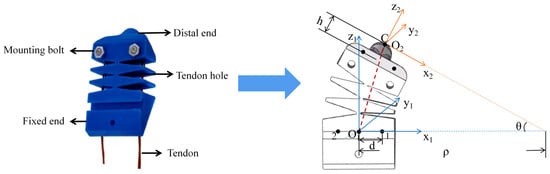
The upper part of the leg serves as a fixed end connected to the body, with through holes on both sides to constrain the transmission path of the tension cable. A continuous central skeleton is used to bear the main load and constrain the bending shape, preventing excessive distortion under stress. A raised support structure at the end of the leg acts as a buffer, reducing the impact of vibrations on the robot’s posture during walking. It also prevents drive components from directly contacting the ground, reducing the risk of wear. The physical structure of the leg is shown in Figure 1.

Figure 1. Cable-driven leg movement.

The blue solid line represents coordinate system o₁x₁y₁z₁, and the orange solid line represents coordinate system o₂x₂y₂z₂. The red dashed line represents the distance from the theoretical endpoint C to the origin O₁. A coordinate system for modeling leg bending is established. The base coordinate system o₁x₁y₁z₁ is established at the center of the fixed end of the leg. The z₁ axis is established along the direction of the central skeletal structure of the leg, the x₁ axis points in the positive bending direction of the leg, and the y₁ axis is determined by the right-hand rule. The end effector coordinate system o₂x₂y₂z₂ is located at the center of the end of the leg, and its posture changes with leg bending. Since the actual end effector mounting position has a fixed offset relative to the theoretical end of the central skeletal structure, the theoretical end effector point C is introduced as a geometric auxiliary point.

2.1. PCC-Based Modelling of Leg Structural Bending

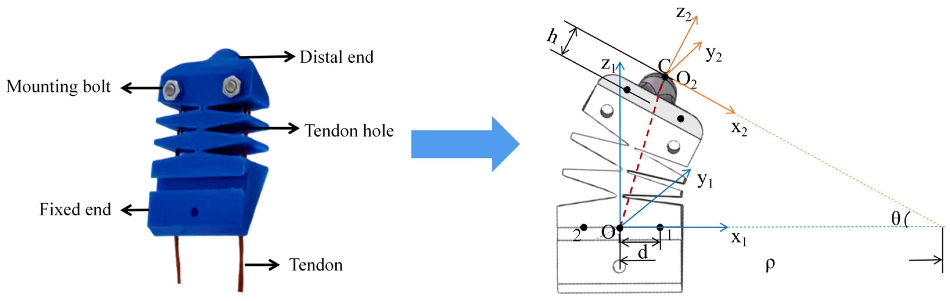
Soft robot exhibit significant nonlinear characteristics during bending deformation, and the relationship between the driving input and the structural response is difficult to describe directly using traditional geometric relationships. The piecewise constant curvature (PCC) method is used to model the robot’s leg. The bending segment of the flexible leg is approximated as a circular arc with constant curvature, and the overall configuration is described by the bending angle. The actuation space is the space of servo motor inputs that drive the cable traction, represented by the servo rotation angle. The configuration space is the space of leg deformation states under the PCC assumption, represented by the leg bending angle. The task space is the space of foot-end positions in the base coordinate system, represented by the position vector of the leg tip. The workspace is the set of all reachable positions of the leg end obtained by varying the bending angle and lifting angle within their admissible ranges. The kinematic mapping relationship of the leg model can be expressed as Figure 2 below.

Figure 2. The relationship between the actuation space, configuration space and task space.

Among these, $\phi$ is the rotation angle of the servo, $\theta$ is the bending angle of the flexible leg, and $p={\left[x,y,z\right]}^T$ is the position vector of the leg’s tip in the base coordinate system.

Figure 2 shows that the servo motor rotation causes the cable to contract, which in turn drives the flexible leg to bend, changing the spatial position of the leg end. The design parameters for the legs are shown in Table 1.

Table 1. Model structure parameters.

Parameters	Initial Values/mm
Height of the leg	55
Length of the leg	30
Width of the leg	13
Central framework (L0)	40
Lateral offset (h)	10
Drive line offset distance (d)	10

Under the PCC assumption, the curved section of the central skeleton can be regarded as a circular arc with constant curvature. Let $L_0$ be the length of the central skeleton, $\theta$ be the bending angle of the flexible leg, $\kappa$ be the equivalent curvature, and $\rho$ be the equivalent radius of curvature. Their relationship is expressed as follows:

$$\kappa ={\displaystyle \frac{\theta }{L_0}}, \rho ={\displaystyle \frac{1}{\kappa }}={\displaystyle \frac{L_0}{\theta }}$$

(1)

Here, $\rho$ is retained only as the equivalent radius of curvature to keep the position equations compact. The position vector $P_c$ of the end point C of the central frame in the base coordinate system is:

$$P_C=\left[\begin{array}{c}\rho \left(1-\cos \theta \right)\\ 0\\ \rho \sin \theta \end{array}\right]$$

(2)

It can be seen that point C always lies in the x₁o₁z₁ plane, and its coordinate along the y₁ axis is always 0. The range of values $\theta$ for θ is determined by the drawback limit of the guy wire and the mechanical constraints of the leg structure. Therefore, $\theta$ is varied only within the physically feasible range. For the straight-leg configuration, the limit form is used to avoid the singularity caused by Equation (1). The limit is given by:

$$\underset{\theta \to 0}{\lim }\rho \left(1-\cos \theta \right)=0,\underset{\theta \to 0}{\lim }\rho \sin \theta =0,P_c\left(0\right)={\left[0,0,L_0\right]}^T$$

(3)

Given that the actual end point o₂ has a fixed offset relative to the theoretical end point C, let the offset vector be defined as follows:

$$r=\left[\begin{array}{c}0\\ h\\ 0\end{array}\right]$$

(4)

When the leg is bent, the end-effector coordinate system rotates about the y₁ axis relative to the base coordinate system. The rotation matrix is as follows:

$$R\left({\mathrm{y}}_1\right)=\left[\begin{array}{ccc}\cos \theta & 0& \sin \theta \\ 0& 1& 0\\ -\sin \theta & 0& \cos \theta \end{array}\right]$$

(5)

Therefore, the position of the actual endpoint o₂ in the base coordinate system can be expressed as:

$$P_{0_2}=P_c+R\left({\mathrm{y}}_1\right)r$$

(6)

Equation (5) describes the mapping from the configuration space to the local task space without expanding each coordinate component separately. The flexion of the flexible leg is driven by the contraction of the tension wire. Let the effective length of the rudder arm be $r_s$, and the change in the length of the drive line be $\mathsf{\Delta }l$. When the servo is rotated by an angle of $\phi$, the control arm moves the control line, causing the length of the drive line to change as follows:

$$\mathsf{\Delta }\mathrm{l}=r_s\phi$$

(7)

The distance $d$ separates the drive line from the central frame. Based on the PCC geometry, the difference in cable length caused by leg bending is:

$$\mathsf{\Delta }l=d\theta$$

(8)

Combining Equations (7) and (8), the relationship between the servo angle and the leg flexion angle is given by:

$$\theta =f\left(\phi \right)={\displaystyle \frac{r_s}{d}}\phi$$

(9)

Equation (8) provides the analytical mapping relationship from the actuation space to the configuration space, indicating that under quasi-static bending conditions, the bending angle of the flexible leg is approximately linearly related to the servo motor rotation angle. Here, r_s determines the amplification effect of the servo motor input on the cable retraction, and $d$ determines the influence of the cable offset on the bending angle generation efficiency.

Substituting this mapping relationship into Equation (5), we obtain the forward kinematic model of the leg end position with respect to the drive input.

$$P\left(\phi \right)=\left[\begin{array}{c}{\displaystyle \frac{L_0}{f\left(\phi \right)}}\left[1-\cos f\left(\phi \right)\right]\\ h\\ {\displaystyle \frac{L_0\sin f\left(\phi \right)}{f\left(\phi \right)\theta }}\end{array}\right]$$

(10)

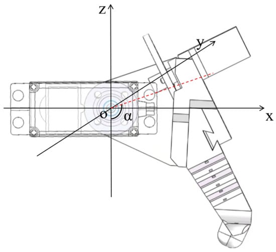
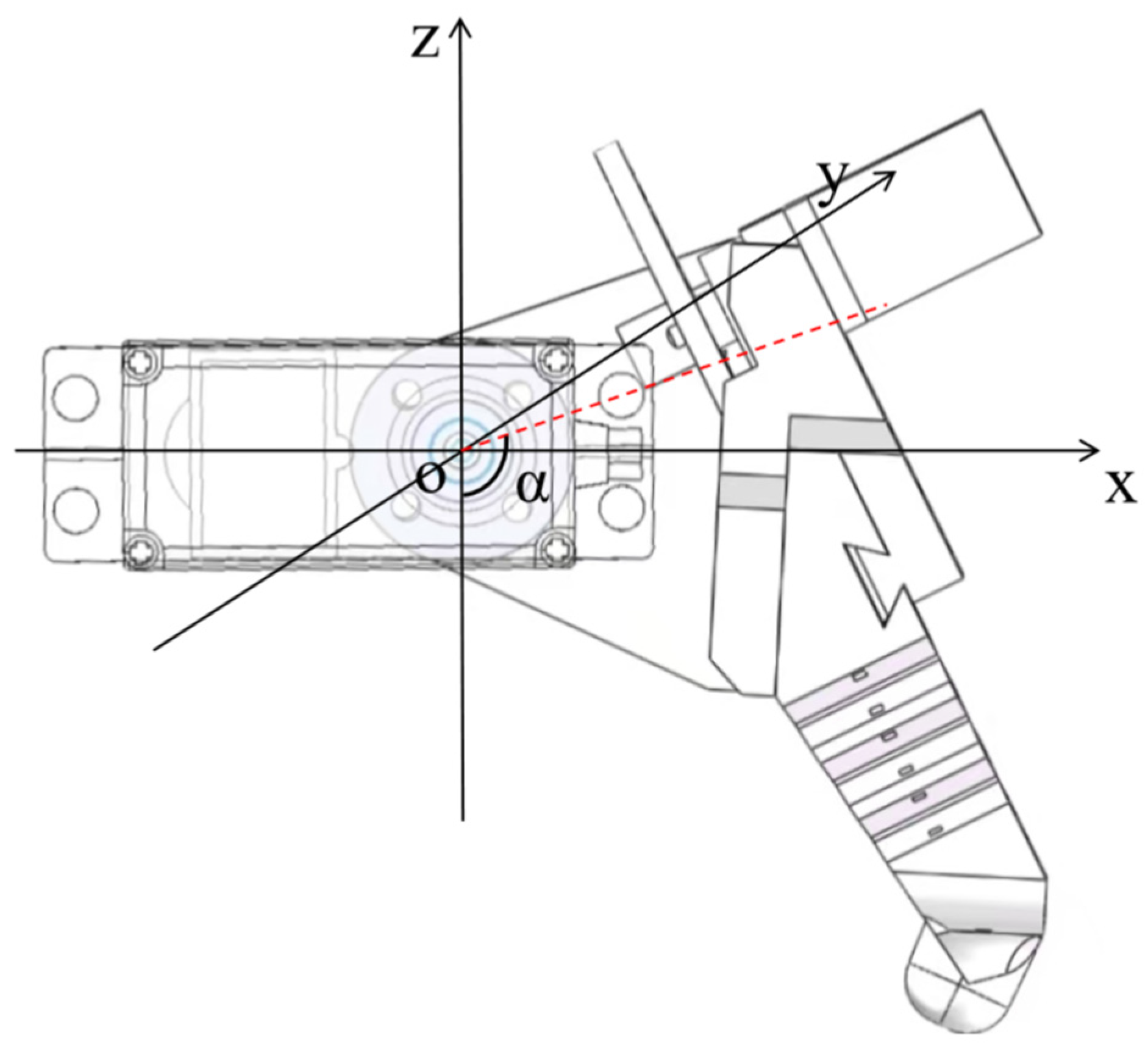
Since the flexible leg is connected to the robot body through a lifting mechanism, the local leg model must be transformed into the global coordinate system OXYZ. As shown in Figure 3, the legs rotate about the Y-axis during lifting, with the angle of rotation denoted as $\alpha$.

Figure 3. Global coordinate system.

The red dashed line in the diagram represents the rotation angle of the lifting structure. When $\alpha =0$, the x-axis of the global coordinate system is aligned with the y₁-axis of the local coordinate system. Let $r_0$ be the installation offset of the leg-raising joint from the global coordinate system.

$${\mathrm{r}}_0={\left[25,0,-20\right]}^T\mathrm{mm}$$

(11)

The rotation matrix for lifting the leg around the Y-axis is as follows:

$$R\left(\alpha \right)=\left[\begin{array}{ccc}\cos \alpha & 0& \sin \alpha \\ 0& 1& 0\\ -\sin \alpha & 0& \cos \alpha \end{array}\right]$$

(12)

The position of the leg’s end in the global coordinate system is as follows:

$$P\left(\theta ,\alpha \right)=R\left(\alpha \right)\left(P^{\prime }\left(\theta \right)+r_0\right)$$

(13)

Expanding this gives:

$$P\left(\theta ,\alpha \right)=\left[\begin{array}{c}(25+h)\cos \alpha +\left(-20+{\displaystyle \frac{L_0}{\theta }}\rho \sin \theta \right)\sin \alpha \\ -{\displaystyle \frac{L_0}{\theta }}\left(1-\cos \theta \right)\\ -(25+h)\sin \alpha +\left(-20+{\displaystyle \frac{L_0}{\theta }}\rho \sin \theta \right)\cos \alpha \end{array}\right]$$

(14)

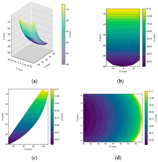
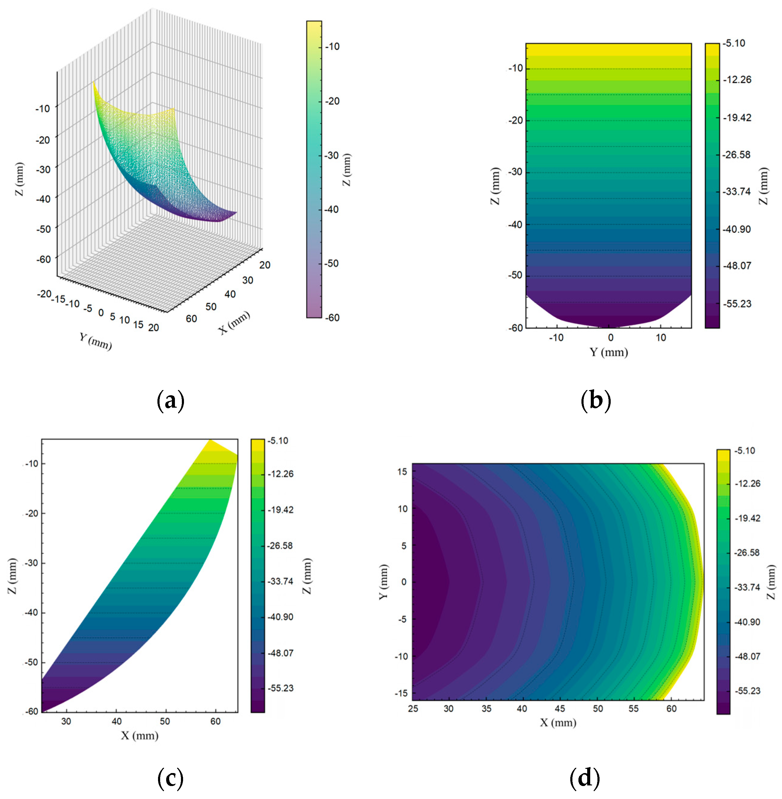
It is evident that the leg posture is determined by both the lifting angle and the bending angle. By iterating through parameter range of $\alpha$ and $\theta$, reachable workspace of the leg end is obtained. The calculated workspace results are shown in Figure 4.

Figure 4. Distribution of the leg model workspace: (a) 3D workspace distribution of the leg model; (b) Distribution of leg model positions on the YOZ plane; (c) Distribution of leg model positions on the XOZ plane; (d) Distribution of leg model positions on the XOY plane.

Colored by z-value, the workspace at the leg end exhibits an approximately fan-shaped distribution, demonstrating good forward extension and lateral coverage. In the YOZ plane, the lateral displacement distribution of the end is symmetrical about the midpoint. In the XOZ plane, the end extends forward, with the z-axis height gradually increasing, and the workspace boundary displays a distinct nonlinear bending characteristic. In the XOY plane, the reachable area exhibits a distribution that is wider at the front and narrower at the back, indicating stronger motion coverage in both forward support and swing directions.

2.2. The Effect of Structural Parameters on Bending Performance

Leg bending performance is jointly controlled by structural stiffness and compliance. Excessive stiffness limits bending output, while excessive compliance reduces load-bearing capacity and causes local stress concentration. The flexible legs were fabricated from TPU 95A filament using fused deposition modeling (FDM) 3D printing. The nozzle temperature was set to 220 °C, with a layer height of 0.2 mm and an infill density of 100%. Each leg was printed in the vertical direction, so that the layer direction was perpendicular to the bending plane. Based on these structural characteristics, a finite element model was established in ANSYS Workbench 2023 R2 and simplified as an isotropic constitutive model. The elastic modulus is taken as E = 30 MPa and the Poisson’s ratio is taken as μ = 0.49 to represent its approximately incompressible mechanical properties [25]. The guy wire is simulated as structural steel with an elastic modulus of E = 210 MPa [26]. Fixed constraints are set at the connection between the guy wire and the fixed hole, and a connecting pair that allows axial sliding is set between the guy wire and the guide hole to reflect the transmission characteristics of the guy wire in the channel. Only normal contact is considered between adjacent surfaces, and tangential friction is ignored. By applying a load along the direction of the guy wire, the traction effect of the guy wire tightening on the leg is simulated.

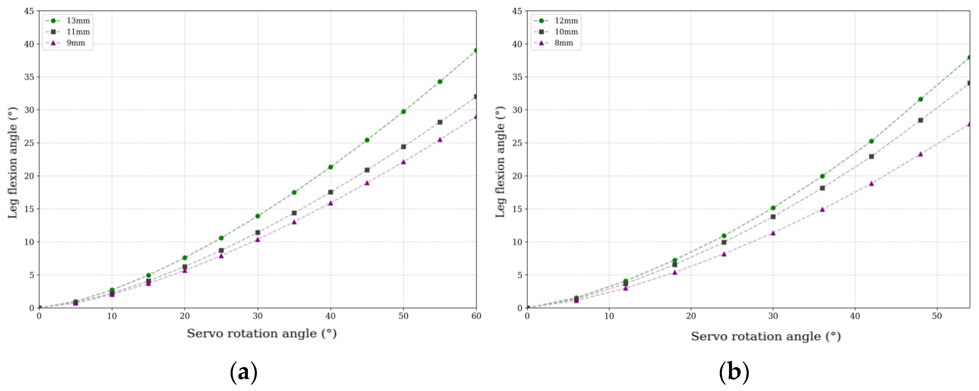
For long-term operation of legged robots, the flexible legs need to balance bending actuation capability and stress safety. The main geometric parameters selected are the mid-layer cut depth configuration, central axis thickness, and wire hole offset distance, and their impact on leg bending performance and stress distribution is analyzed. The cut depth directly affects compliance and bending deformation capability; different depths of 9 mm, 11 mm, and 13 mm are compared. The wire hole offset distance affects the bending moment by changing the driving arm; 8 mm, 10 mm, and 12 mm are analyzed. The changes in leg bending angle under different parameters are shown in Figure 5.

Figure 5. Analysis of leg flexion performance: (a) Analysis of leg bending performance under different middle-layer notch depths; (b) Analysis of the effect of draw hole offset distance on leg bending performance.

As shown in Figure 5a, the leg bending angle at different cut depths shows a continuous upward trend. The bending angle corresponding to a cut depth of 13 mm is consistently higher than that of 11 mm and 9 mm, indicating that deepening the cut effectively reduces the local stiffness of the intermediate layer, thereby promoting leg bending output. Therefore, 13 mm is selected as the intermediate layer cut depth. As shown in Figure 5b, as the offset distance of the draw hole increases, the bending moment strengthens, and the leg bending response becomes more pronounced. The bending angle is largest at an offset distance of 12 mm, and the bending output is lowest at an offset distance of 8 mm. The 10 mm scheme falls between the two and provides a relatively significant bending response. By comprehensively comparing the bending output and stress state under different offset distances, it is determined that the draw hole is located 10 mm from the central axis.

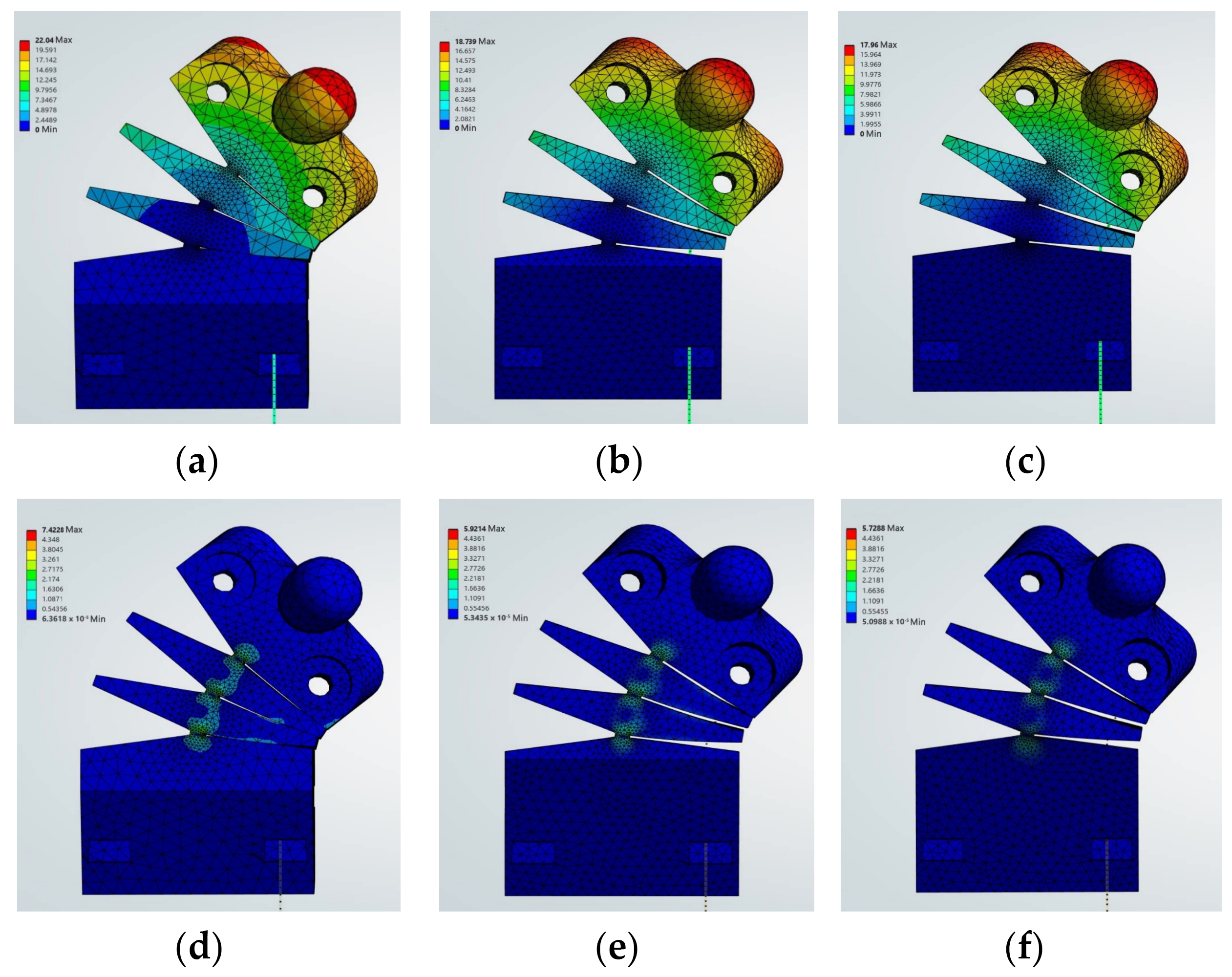
As the main load-bearing component of the legs, the size of the central shaft directly affects the overall stiffness and bending response, with the thickness having a more significant impact. With other parameters and load conditions remaining constant, three models were established with central shaft thicknesses of 10 mm, 13 mm, and 16 mm, respectively. The total structural deformation and equivalent stress distribution results are shown in Figure 6.

Figure 6. Total deformation and equivalent stress distribution for different thicknesses: (a) Total deformation result for central axis thickness of 10 mm; (b) Total deformation result for central axis thickness of 13 mm; (c) Total deformation result for central axis thickness of 16 mm; (d) Stress distribution results for central axis thickness of 10 mm; (e) Stress distribution results for central axis thickness of 13 mm; (f) Stress distribution results for central axis thickness of 16 mm.

In images (a), (b), and (c), the blue areas represent simulated rope pulling. The overall deformation results show that all three models exhibit bending deformation, with the deformation concentrated in the middle layer region. The model with a central axis thickness of 10 mm shows the most significant deformation. However, Figure 6e shows that the 10 mm scheme has localized areas of high stress concentration, which may lead to structural failure under load. The 16 mm scheme has a more uniform stress distribution, but the overall deformation is smaller. Comprehensive analysis concludes that the 13 mm scheme achieves a better balance between bending performance and load-bearing safety.

2.3. Finite Element Bending Simulation

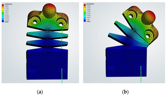
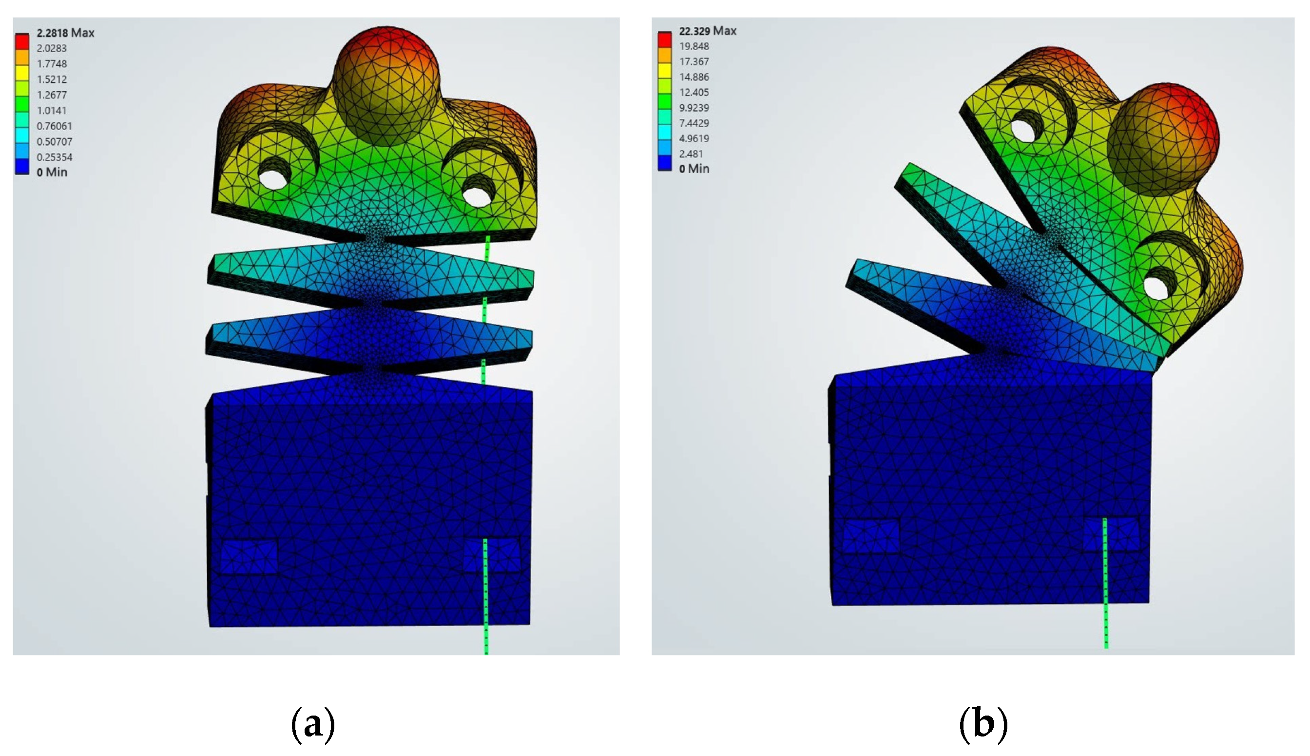
Apply displacement load along the axial direction of cable to simulate the bending deformation process of the robot’s leg. The structural configurations at the initial state and the maximum load state are selected for comparison, as shown in Figure 7.

Figure 7. Finite element bending simulation of leg model: (a) Initial state of the leg when no force is applied; (b) The leg condition under maximum load.

In the figure, the blue areas represent simulated rope pulling. In the initial state, the leg is not pulled by the string and remains naturally extended. As the string continues to tighten, the middle section gradually compresses. When the load is at its maximum, the leg is bent to its fullest extent, transitioning from its initial upright position to a noticeably bent state.

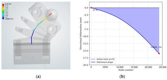
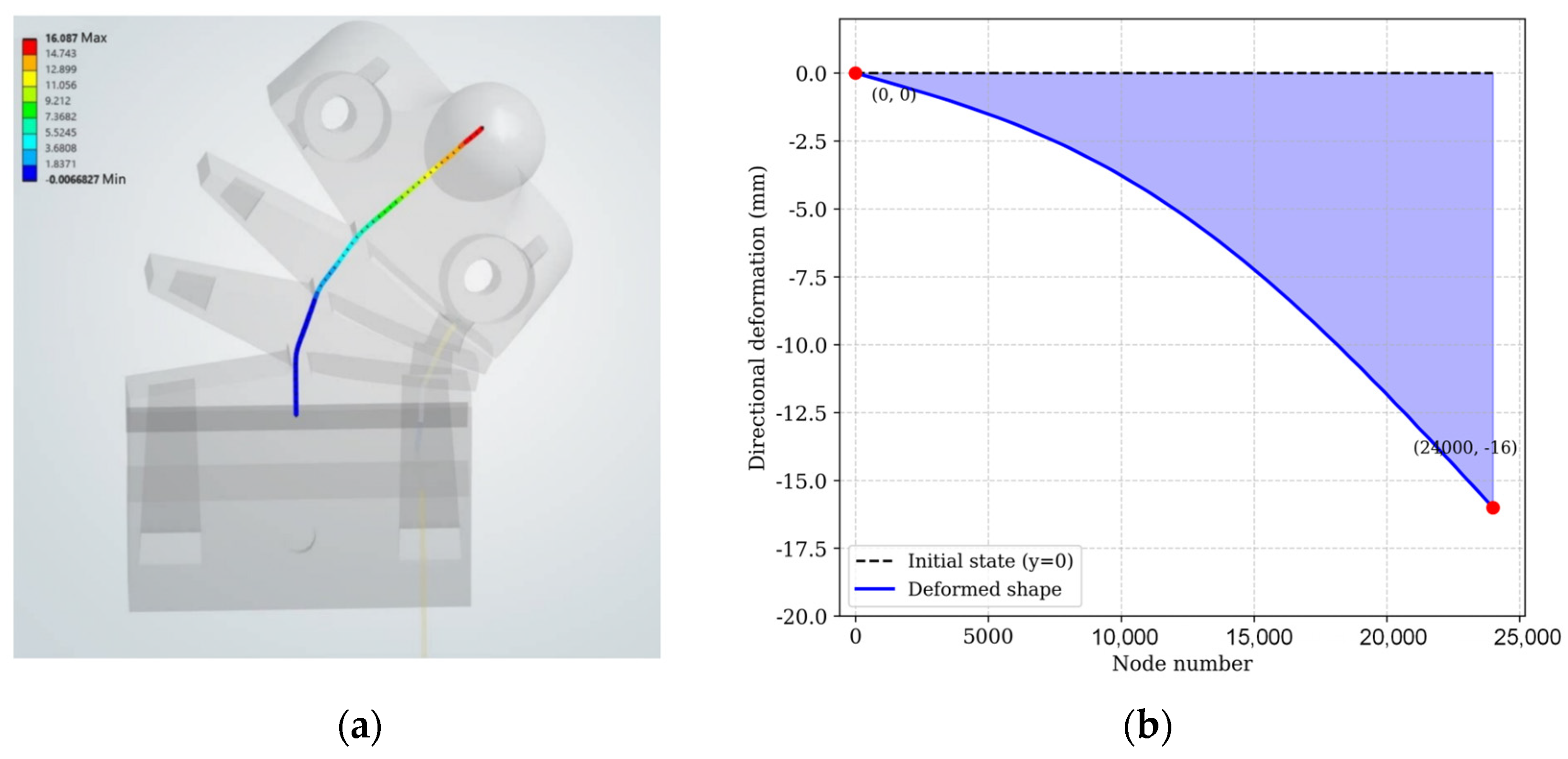
Under maximum load conditions, a series of nodes are selected along the length of the flexible leg’s central axis, and the displacement components of each node in the principal bending direction are extracted. As shown in Figure 8a, the directional displacement of the nodes gradually increases along the central axis; the displacement is smaller in the bottom fixed region, whilst the effect of the tensile cable pulling is more pronounced in the upper region, where the displacement reaches its maximum value. Under the driving force of the cable, the flexible leg undergoes continuous bending deformation along the central axis, consistent with the actual bending behaviour. Based on the extracted node displacement data, a distribution map of the directional deformation at each node is plotted. As shown in Figure 8b, the node number is plotted on the x-axis, and the corresponding directional displacement of the node in the bending direction is plotted on the y-axis.

Figure 8. Analysis of joint deformation and displacement under maximum load: (a) Displacement results of nodes along the central axis in the bending direction; (b) Distribution of directional deformation of nodes along the central axis.

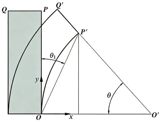
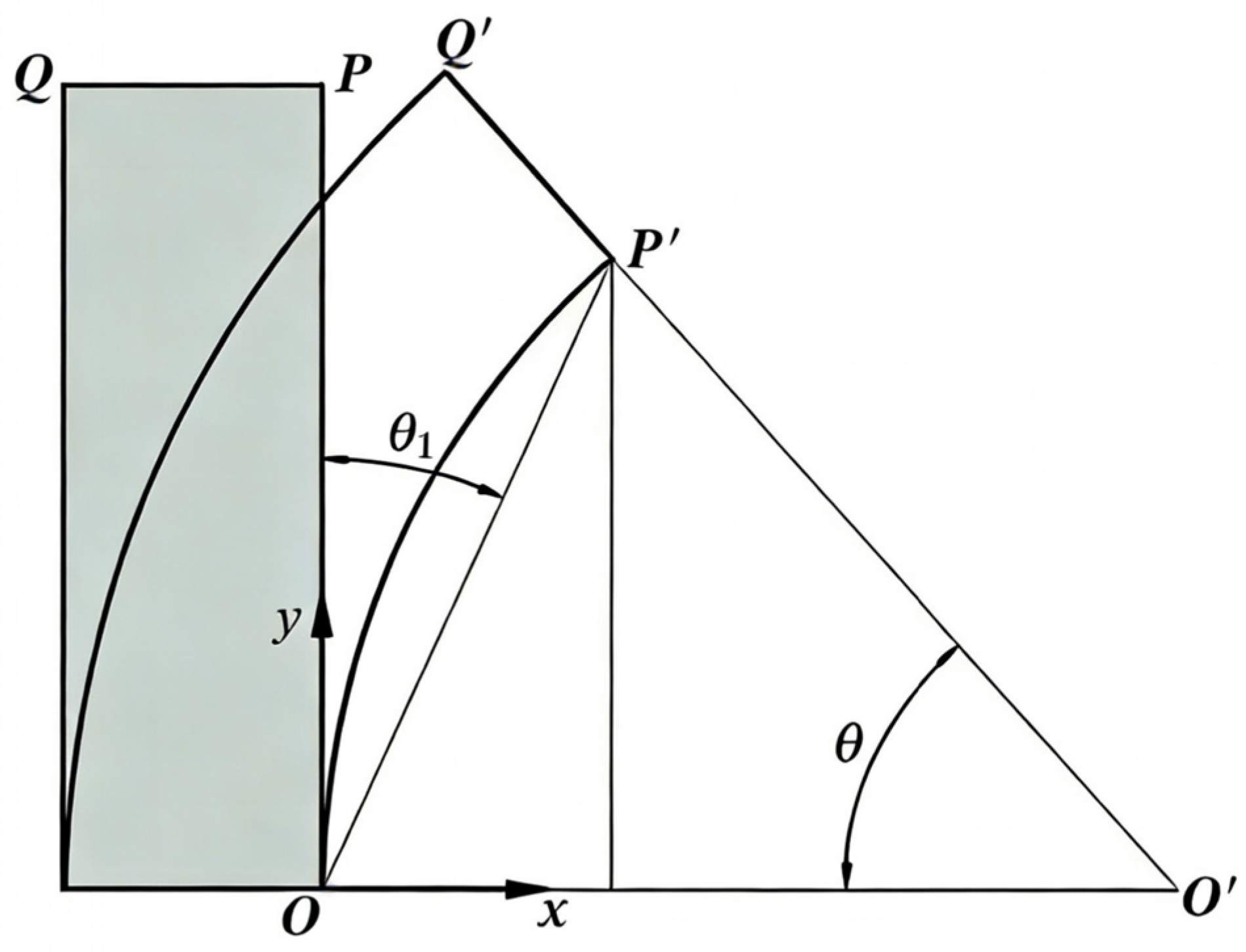
Along the central axis of the leg, the displacements of the selected nodes generally increase in a continuous and smooth manner. Therefore, the end node is selected as the characteristic point for calculating the bending angle. In the initial state, point P lies on the vertical centerline of the leg, and its coordinate is written as P(0, y1). After deformation, the corresponding point moves to P′(x2, y2), as shown in Figure 9.

Figure 9. Leg bending exercise diagram.

In Figure 9, ${\theta }_1$ denotes the local bending angle of the flexible leg, defined as the angle between the initial vertical direction of the leg and the line connecting the fixed point O to the deformed characteristic point P′. ${\theta }_1$ is used only to illustrate the measured bending angle in the deformation diagram.

The leg bending angle is calculated using the geometric relationship between the vectors pointing towards the central axis before and after deformation. The geometric formula is as follows:

$$\theta =\arccos \left({\displaystyle \frac{{\mathrm{y}}_2}{\sqrt{x_2^2+y_2^2}}}\right)$$

(15)

3. Robotic Structure Design and Control Implementation

In nature, ants are typical six-legged creatures, with their bodies consisting of a head, thorax, and abdomen, and their center of gravity mainly concentrated in the thorax region. When traversing rugged and uneven ground, ants can maintain their balance by adjusting the landing point of their legs and their stride [27]. Based on this biological characteristic, this study adopts a bilaterally symmetrical six-legged overall configuration, enabling the robot to form multi-point support during movement and improving its potential motion stability under uneven terrain conditions.

3.1. Robot Control Platform Setup

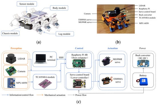
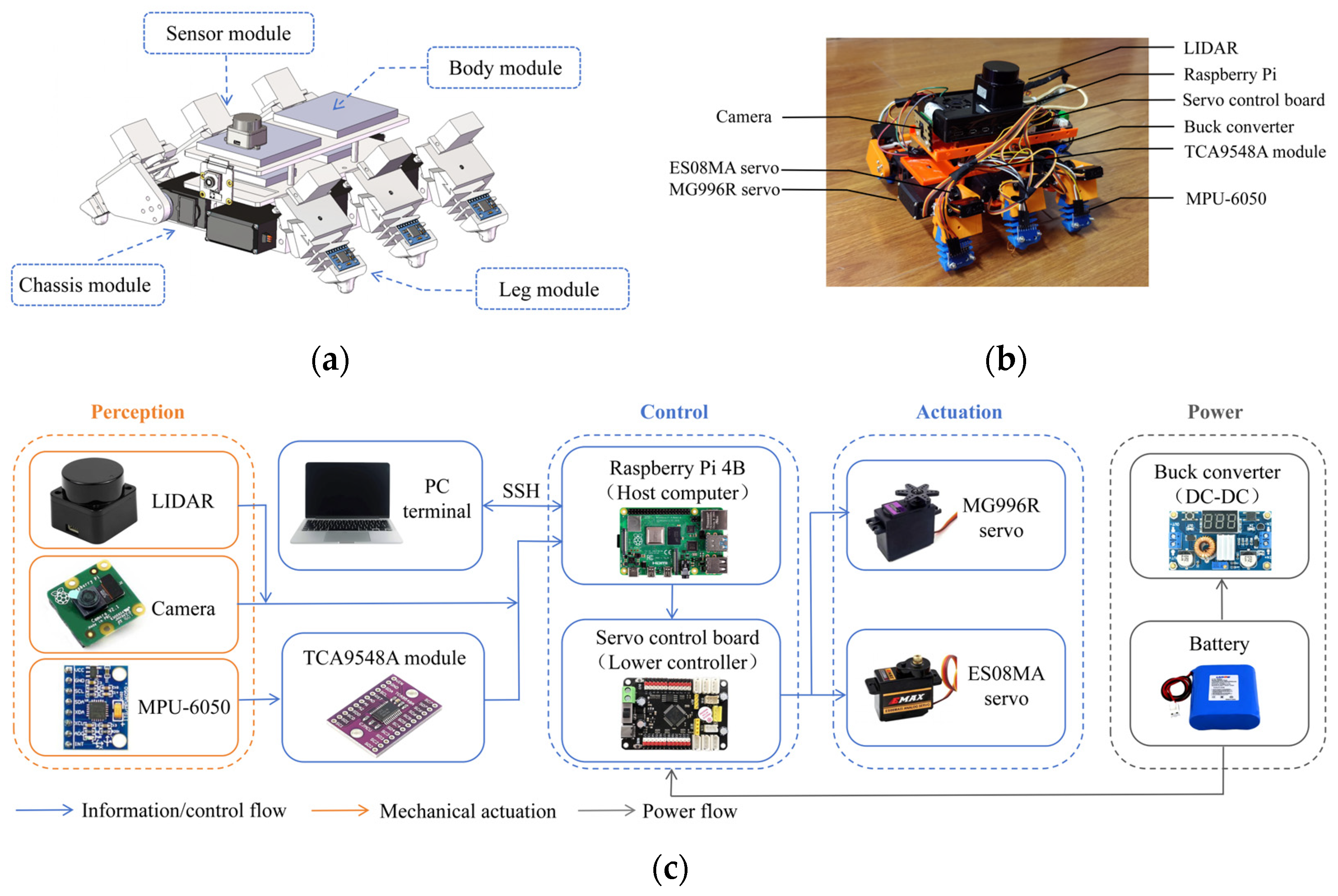
The robot’s compliant leg deformation was combined with its foot-like motion, and a 3D model of the robot was created using SolidWorks 2023 software. The design of the robot control platform is shown in Figure 10.

Figure 10. Construction of the control platform for the hexapod robot: (a) 3D model of the robot; (b) Robot prototype setup and equipment layout; (c) Control and perception architecture of the ROS-based system.

Figure 10a shows the four main components of the robot: sensor module, body module, chassis module, and leg module. As shown in Figure 10b, the robot platform is constructed with overall dimensions of 210 mm × 200 mm × 250 mm. The robot weighed 870 g, including the body frame, servomotors, sensors, and battery. The robot uses its body as the core support platform, with three flexible legs on each side, forming a symmetrical six-legged structure. The lower layer houses the servo motors and leg connection components, while the upper layer serves as the electronic equipment mounting platform, housing the controller, sensors, and related circuit modules.

Each leg is driven collaboratively by an MG996R servo motor and an ES08MA servo motor, enabling two degrees of freedom of movement per leg. The MG996R servo motor lifts the leg, while the ES08MA servo motor drives the flexible leg to bend forward and backward via a cable. Powered by a 7.4 V lithium battery, the MG996R draws approximately 0.8 A under load and the ES08MA approximately 0.3 A. The total power consumption of the actuation system can be estimated as:

$$P=6\times V\left(I_{MG996R}+I_{ES08MA}\right)$$

(16)

In the equation, $V$ is the supply voltage, and $I_{MG996R}$ and $I_{ES08MA}$ are the operating currents of the two servomotor types. Substituting the values gives $P=48.8 W$.

As shown in Figure 10c, the robot control system adopts a layered architecture. The PC connects to a Raspberry Pi 4B via SSH for remote monitoring and program debugging. The Raspberry Pi 4B acts as the host computer, responsible for processing multi-source sensor data and generating motion control commands. Simultaneously, the Raspberry Pi 4B communicates with the servo motor control board via a serial port, with the control board outputting PWM signals to drive the servo motors.

The perception system is configured to collect environmental and attitude information for monitoring, SLAM, and visualization. LiDAR and cameras complement each other in terms of the information they provide, capturing environmental distance data and visual images respectively to describe the spatial conditions surrounding the robot. LiDAR, which operates on the Time of Flight (TOF) principle, enables environmental distance perception by calculating the distance to an object through the measurement of the time difference between the emission and reception of light.

$$\mathrm{d}={\displaystyle \frac{ct}{2}}$$

(17)

Among these, d represents the distance to the target, c represents the speed of light, and t represents the round-trip propagation time of the laser signal; the measured time corresponds to the total time taken for the laser to travel from the transmitter to the target and back to the receiver via reflection from the target.

The MPU-6050s are mounted on the robot’s legs to collect motion posture data. To avoid address conflicts when multiple MPU-6050s are connected to the I2C bus, a TCA9548A multiplexer is used. After system startup, environmental checks, workspace loading, and parameter file reading are performed sequentially, and the IMU, LiDAR, and camera nodes are started simultaneously to achieve synchronous data transmission from multiple sensors.

3.2. Robot Gait Planning

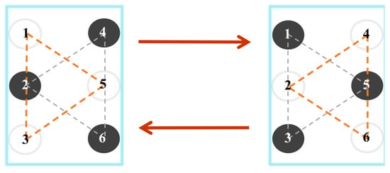
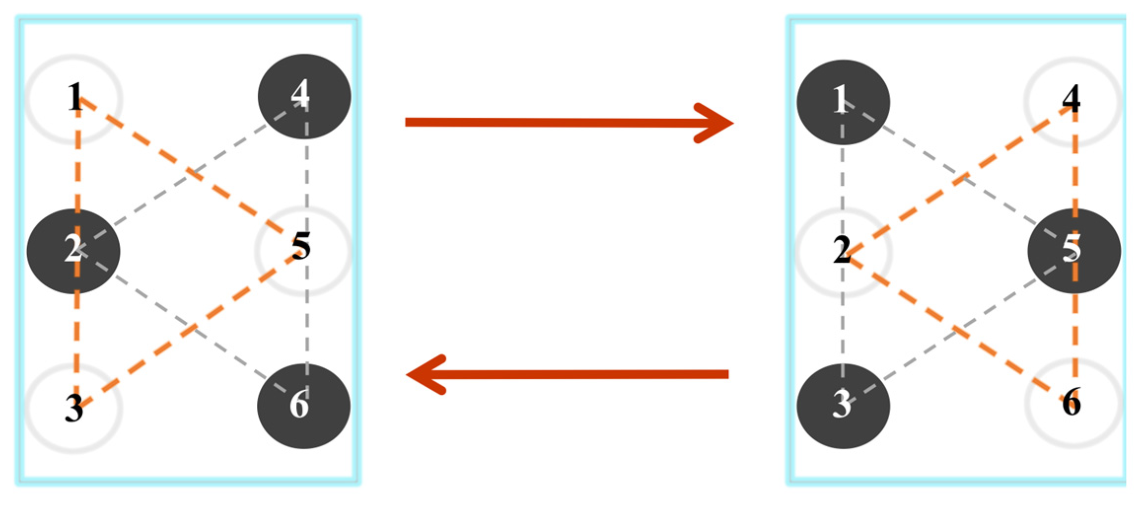
The hexapod soft robot walks in a triangular gait. Figure 11 shows a schematic diagram of the robot’s gait.

Figure 11. Schematic diagram of foot movement based on triangular gait.

Figure 11 illustrates the spatial relationship of the six legs. Orange dashed lines represent oscillation phases. Gray dashed lines represent support phases. The legs are grouped into threes, representing the support phase and the swinging phase respectively. Legs numbered 1, 3, and 5 form one group, and 2, 4, and 6 form another. Each group consists of legs in different positions: front, middle, and rear. Black circles indicate the leg is in the support phase, and white circles indicate the leg is in the swing phase. During tripod gait locomotion, three legs remain in the support phase at any time. The static load on each supporting leg is approximately 290 g. The realization of the robot’s walking gait depends on the effective control of 12 joints.

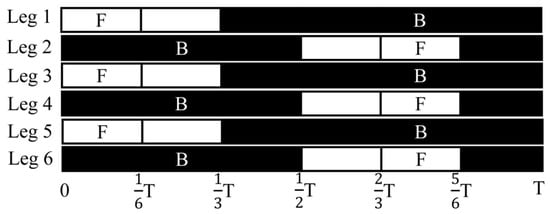
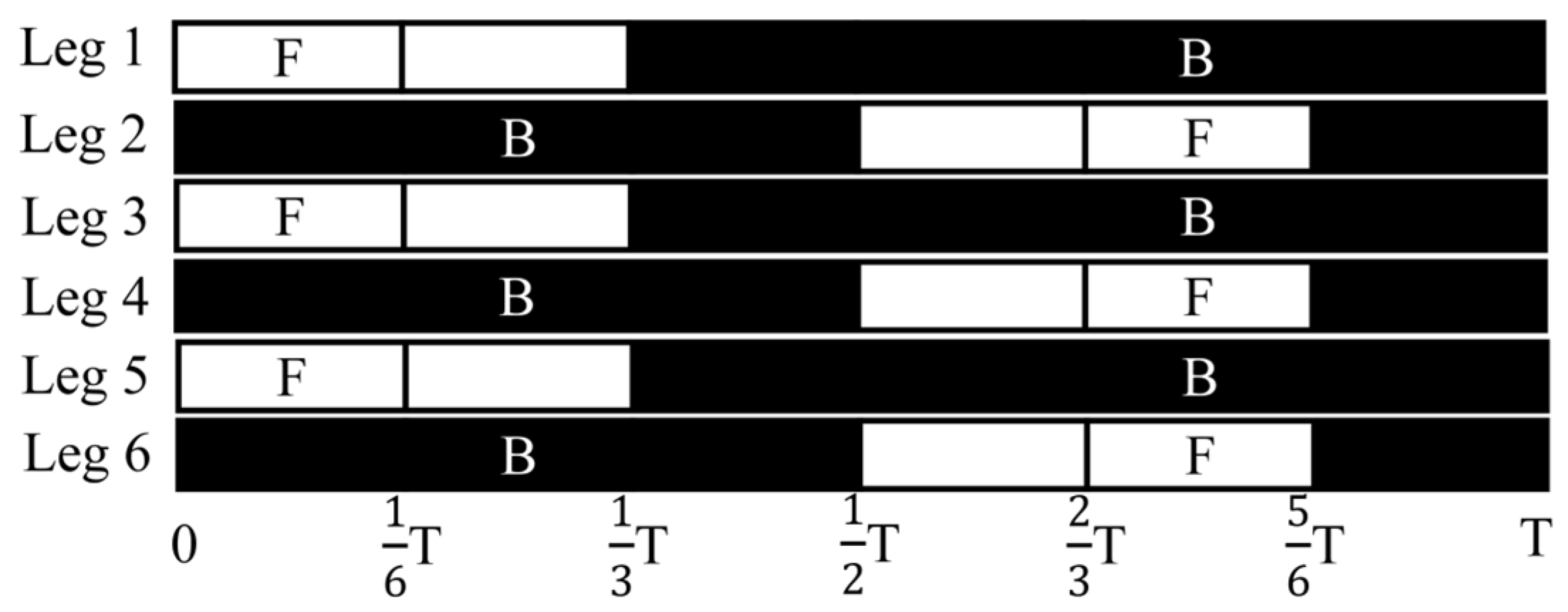
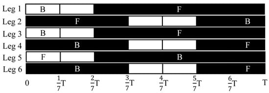
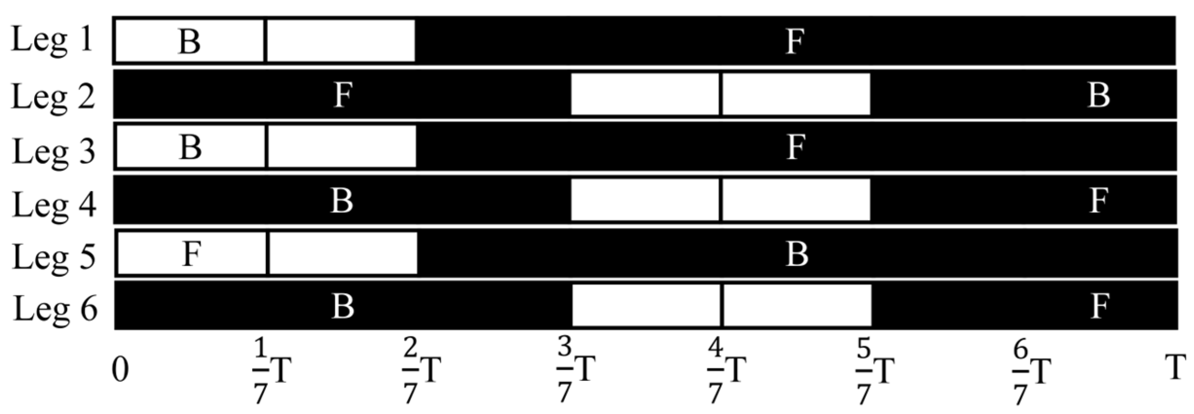
During robot movement, a fixed phase difference is maintained between the two sets of legs, which alternately enter the support phase and the swing phase. Propulsion is generated through the interaction between the feet and the ground, thus converting periodic motion into continuous forward displacement of the body. The gait timing of the robot when moving in a straight line is shown in Figure 12.

Figure 12. Timeline of forward walking gait.

The black areas represent the support phase, and the white areas represent the swing phase. In the diagram, F and B represent the forward and backward bending movements of the lower leg under the drive of the cable, respectively. T is the period of one gait cycle, and the fractional labels, such as 1/6T, 1/3T, and 1/2T, indicate the corresponding normalized time points within the cycle. Within a gait cycle, the robot alternately completes the “swing-landing-support-propulsion” process according to a predetermined phase relationship, enabling it to achieve continuous straight-line movement while maintaining stable support.

The key to a robot’s turning motion lies in adjusting the bending direction and propulsion distribution of its left and right legs. Taking a left turn as an example, the timing sequence of the robot’s left turn motion within one cycle is shown in Figure 13.

Figure 13. Timeline of turning gait.

It can be seen that the calves on both sides adopt different flexion patterns during the same phase of movement, creating an asymmetrical propulsive force on the left and right sides of the body, thereby generating a yawing moment to effect a left turn.

3.3. SLAM-Based Mapping and Localisation

ROS (Robot Operating System) provides a modular and distributed software development framework for robot systems. This paper builds a robot communication and control system based on ROS, dividing sensor data acquisition, motion control, state monitoring, and mapping into relatively independent nodes to improve debugging efficiency.

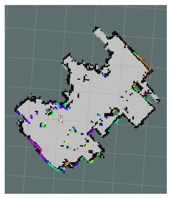
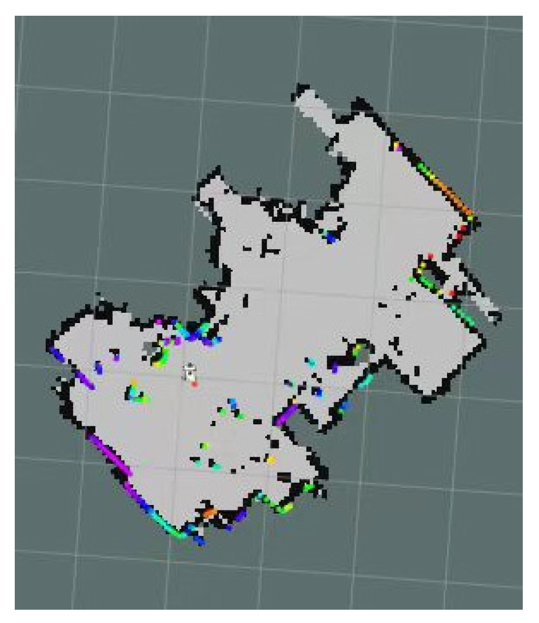
On the PC, sensor data released by the Raspberry Pi is subscribed to and further used for environmental mapping and spatial representation. The SLAM method is used to support two-dimensional mapping and visualization of the experimental environment. The LiDAR continuously outputs scan data of the surrounding environment during robot movement. The Cartographer node is activated, and the system estimates the robot’s position and attitude changes in the plane by matching the LiDAR scan results at consecutive time points. Subsequently, the scan data at each time point are transformed to a unified coordinate system according to their corresponding positions and continuously superimposed and updated to finally form an environmental occupancy grid map.

Using the RViz visualization tool, the mapping process and system operation status are displayed intuitively. Figure 14 shows the LiDAR scan data and the mapping results.

Figure 14. SLAM results.

The light gray area represents the completed environment, while the black areas represent the boundaries of walls or obstacles, indicating that the system can reconstruct the planar outline of the experimental environment relatively completely. The colored dots distributed near the boundaries represent the real-time perception results of obstacles by the LiDAR during scanning, and are marked with different colors. The colored dots are generally distributed along the environmental outline and are largely consistent with the black boundaries, indicating that the LiDAR scanning data matches the map, and the SLAM process is generally stable.

4. Robot Motion Performance Experiment

4.1. Cable-Driven Leg Bending Experiment

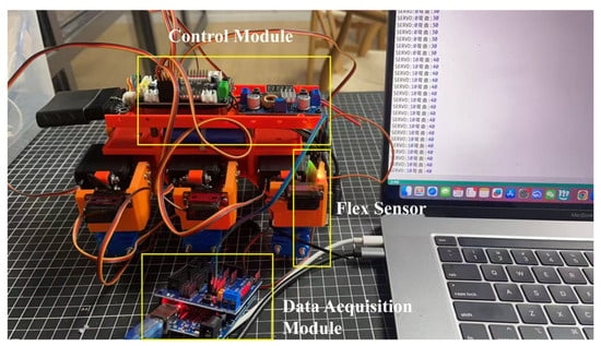
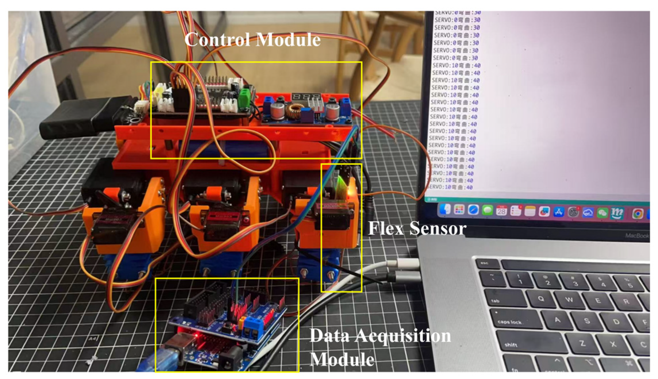
With the robot stationary on the table, and ensuring that the structural configuration and drive conditions remain consistent, one leg was selected as the test subject to avoid coupling interference caused by multi-leg coordinated motion. As shown in Figure 15, a Flex Sensor 2.2-inch unidirectional bending sensor was securely mounted on the surface of this leg. A sensor signal acquisition module was constructed using an Arduino UNO R3 and a V5.0 sensor expansion board. The analogue voltage signal output by the sensor was converted to digital form and transmitted via a USB serial port to a PC, where it was displayed in real time on the serial monitor interface of Mixly 2.0 RE4 for Arduino AVR.

Figure 15. Robotic leg bending test platform.

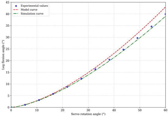
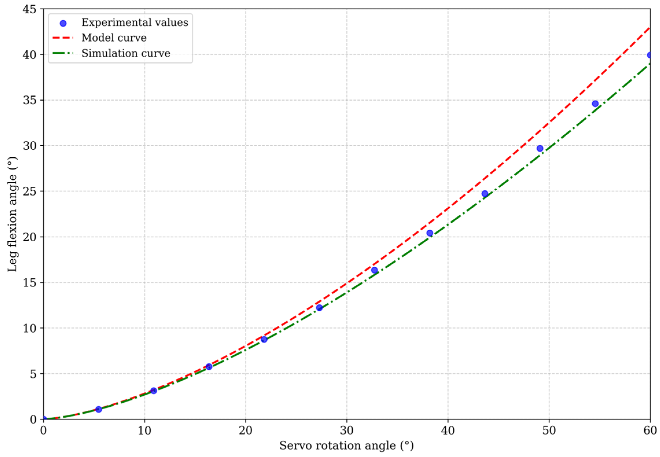
The Chinese label “弯曲” indicates the rotation angle of the servo motor. PC sends control commands to the servo motor, driving it to rotate and bending the leg via a cable. Simultaneously, a bending sensor fixed to the target leg deforms, and its output signal changes with the leg’s bending state. Based on experimental data, a curve showing the relationship between the leg bending angle and the servo motor’s rotation angle was plotted and compared with theoretical models and finite element simulation results. The comparison results are shown in Figure 16.

Figure 16. Comparison of model curves, experimental values, and simulation curves.

The experimental results, model curves and simulation curves show a consistent overall trend; the leg bending angles all increase as the servo angle increases, indicating that the cable-driven structure exhibits a relatively stable bending response. Within a small range of angles, the three show good agreement, with the experimental data points generally distributed in the vicinity of the model and simulation curves. As the servo angle gradually increases, a certain deviation emerges between the experimental values and the model and simulation values. The primary causes of this deviation include material non-linearity, cable transmission backlash, assembly errors, and sensor measurement errors.

4.2. Robotic Physics Experiment

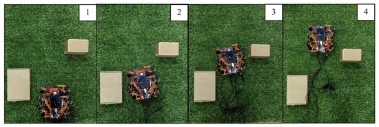
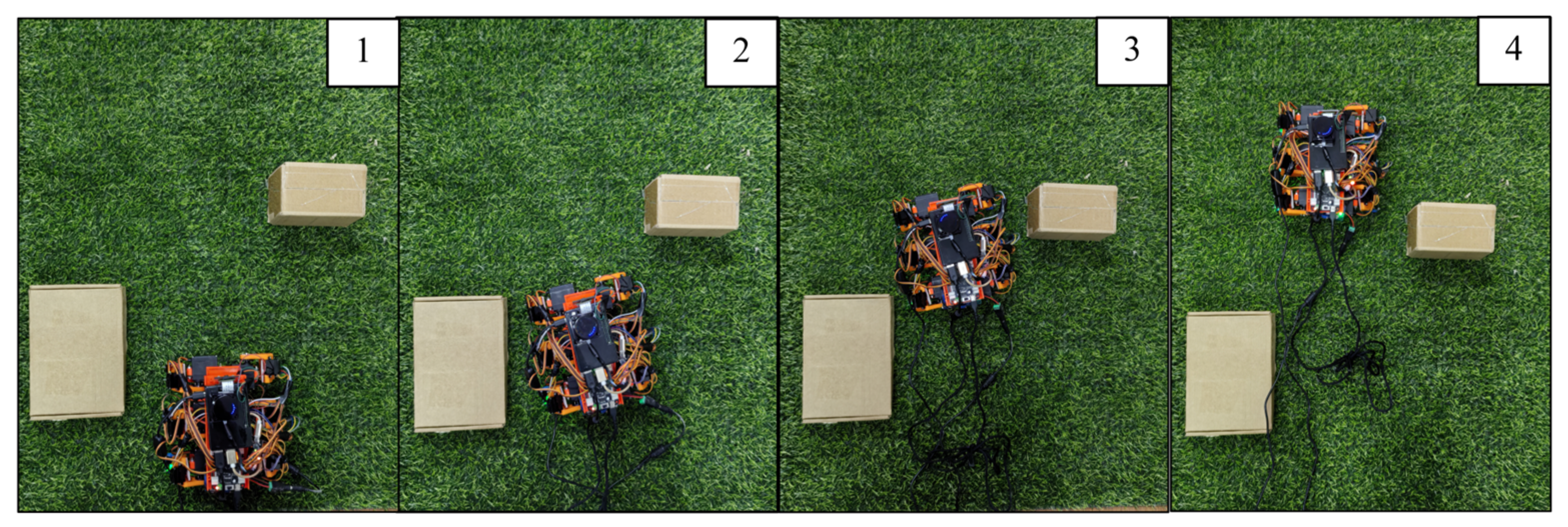
Robots are susceptible to factors such as uneven surfaces and external obstacles whilst in motion. To further validate the robot’s actual performance on uneven ground, two typical terrain types-lawn and gravel paths-were constructed in a laboratory setting. In the following experiments, each trial was repeated 10 times, and the standard deviation and measurement dispersion were used to quantify the dispersion of the measurements. The standard deviation reflects how much a single measurement is dispersed around the mean, while measurement dispersion (defined as the ratio of the standard deviation to the mean) characterizes the relative dispersion of the data. The smaller the values of these two indicators, the higher the repeatability and the better the motion stability of the robot. As shown in Figure 17, obstacles are placed in the lawn scene to simulate obstacle avoidance. Start the Cartographer SLAM node and use the /odom command to record the robot’s pose to calculate its velocity. Record the robot’s position coordinates and timestamp in each trial, and calculate the average velocity as the total path length divided by the elapsed time.

Figure 17. Obstacle course on grass.

The numbers “1–4” in the image indicate the sequence of the robot’s movements. It can be seen that the robot is capable of performing continuous obstacle-avoidance manoeuvres on the lawn. As the surface of the lawn is soft and uneven in places, the foot contact process is susceptible to fluctuations in friction and instability in support. To evaluate the repeatability of the locomotion performance, the experiment was repeated 10 times, yielding an average speed of 15.32 mm/s with a standard deviation of 0.48 mm/s (measurement dispersion = 3.13%). Despite the uneven lawn surface, the robot maintained consistent locomotion speed across repeated trials.

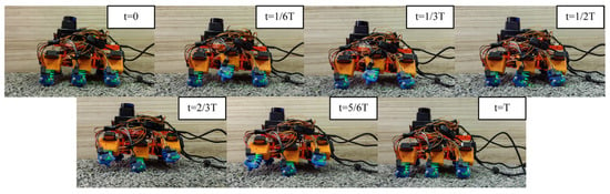
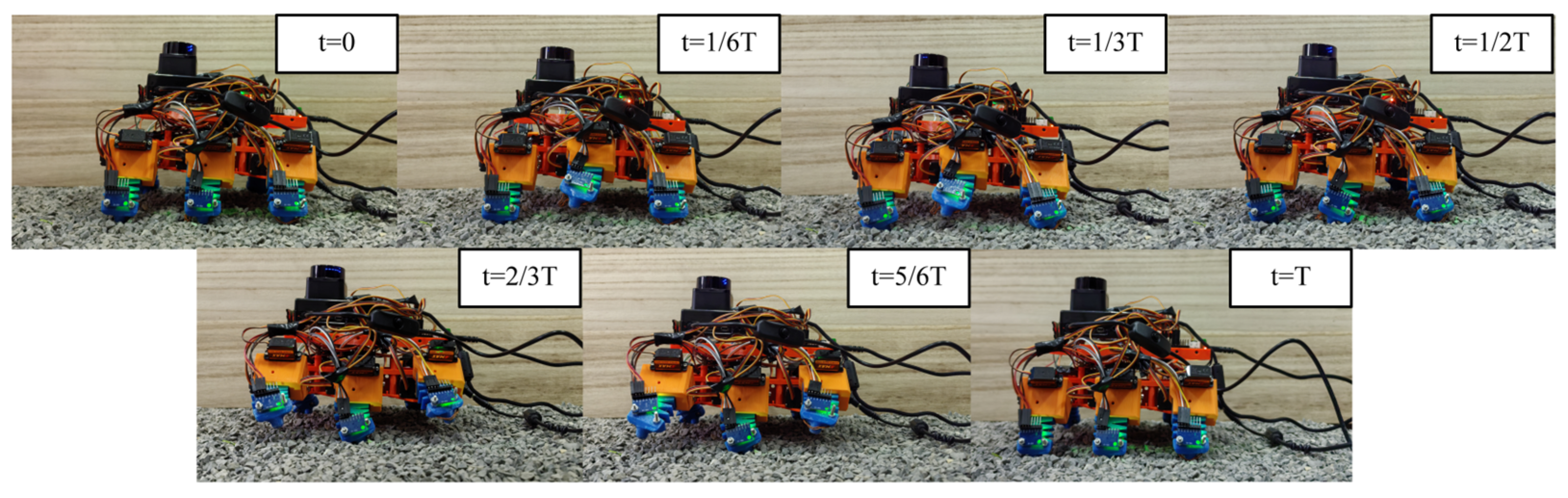
Gravel particles can affect the point of contact at the robot’s foot, making it prone to localised slippage during the stance phase. As shown in Figure 18, we constructed a gravel road environment to record the robot’s movement on the gravel surface during one gait cycle.

Figure 18. Exercises on gravel surface.

The frame sequence shown in the figure illustrates the robot’s alternating support movement, with an average speed of 15.07 mm/s and a standard deviation of 0.63 mm/s (measurement dispersion = 4.18%). The robot smoothly alternated between the support and swing legs, with no noticeable stalling or lateral deviation observed during the movement. This demonstrates that triangular gait and compliant contact can, to a certain extent, adapt to loose and uneven terrain.

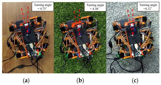
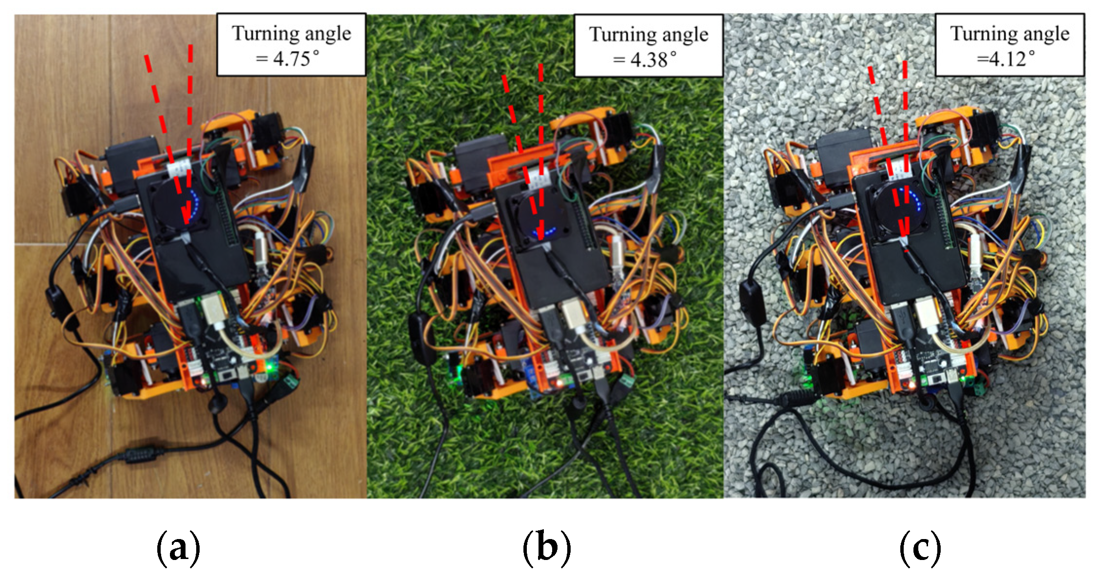
To further evaluate the robot’s steering performance on different terrains, we conducted turning experiments within a single gait cycle. As shown in Figure 19, the robot performed left turns on flat ground, gravel ground, and grass. The yaw values before and after the turn were extracted from the SLAM odometry, and the turning angle was taken as the difference between the two yaw values. The red dashed line represents the change in heading from the initial direction to the direction after the turn, and the corresponding turning angle is marked in the upper right corner.

Figure 19. Turning experiment of robot on different road surfaces: (a) Turning experiment of robot on smooth ground; (b) Turning experiment of the robot on the lawn; (c) Turning experiment of the robot on a gravel road.

The results show that the robot is capable of performing left turns on all three types of ground, with turning angles of 4.75°, 4.38° and 4.12° per gait cycle, with standard deviations of 0.16°, 0.19°, and 0.21° (coefficients of variation of 3.37%, 4.34%, and 5.10%), respectively. Data shows that the filament-driven hexapod robot can perform repeatable turning maneuvers on surfaces with varying degrees of flatness.

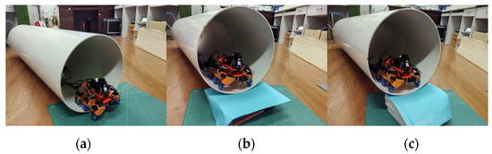
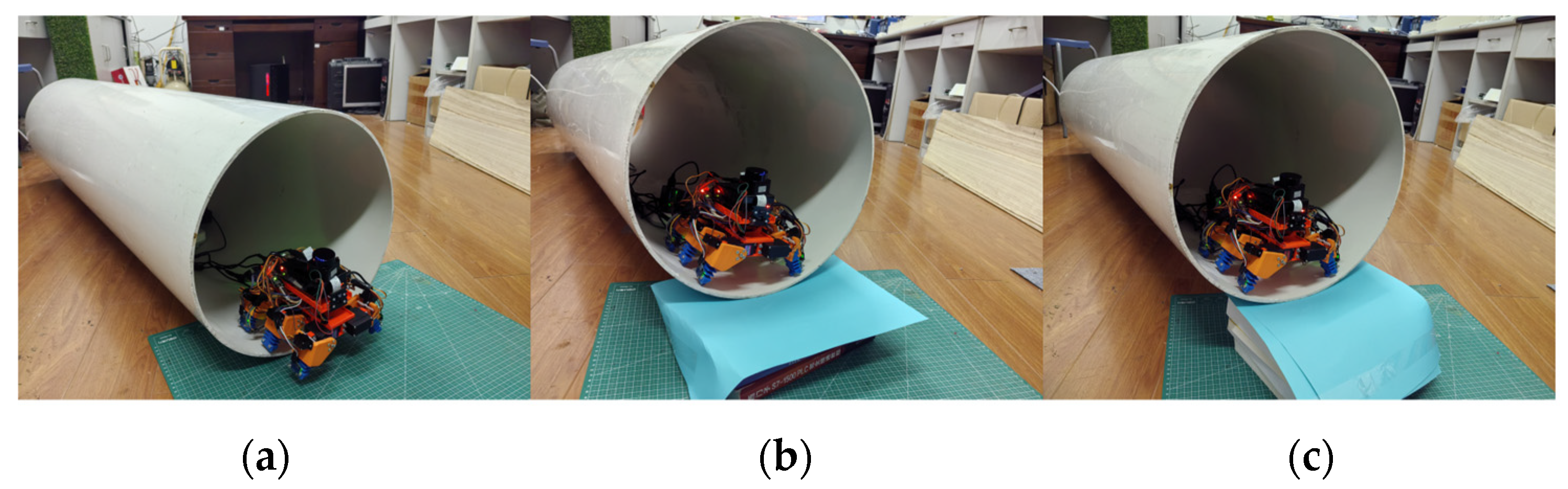
Pipes are one of the most common application scenarios for robots. This study conducted slope-climbing experiments with the robot in a pipe environment to verify its climbing performance on curved surfaces. The pipe was 1.5 m long with a radius of 400 mm. Experiments were carried out to test the robot’s ability to move in a straight line, as well as to climb slopes of 10°and 15°within the pipe. As shown in Figure 20, the experimental setup was constructed such that the robot started at the bottom of the ramp and moved upwards along the ramp under the same control scheme. Each pipe experiment was repeated 10 times.

Figure 20. The robot’s climbing motion inside the pipe: (a) The robot climbs an incline inside a horizontal pipe; (b) The robot climbs a slope inside a 10° pipe; (c) The robot climbs a slope inside a 15° pipe.

On the horizontal pipe (0°), the robot moved at an average speed of 14.85 mm/s (standard deviation = 0.47 mm/s), close to its speed on flat ground. On the 10° slope, the robot still moved steadily but slightly slower, at 12.53 mm/s (standard deviation = 0.56 mm/s) with a 100% success rate. On the 15° slope, the robot showed obvious signs of struggle. The average speed dropped to 10.21 mm/s (standard deviation = 0.69 mm/s), and the success rate fell to 80% (8 out of 10 attempts). At this angle, the foot ends slipped and the robot slid backward during the support phase, so that part of the forward displacement gained in each gait cycle was lost. Compared with the flat-ground speed, the robot’s speed in the pipe decreased. This is mainly because the curved inner surface of the pipe reduced the effective contact area of the feet. As the slope increased, the propulsion resistance at the foot end rose and local slippage occurred, which further reduced the speed.

LiDAR is used for environmental mapping, combined with cameras to capture visual data. Figure 21 shows the SLAM results and the perception of the pipeline environment in RViz.

Figure 21. Mapping the pipeline environment.

The colored dashed lines represent obstacles identified by the lidar. RViz generates a clear map of the pipeline environment, with the LiDAR capable of identifying the inner walls of the pipeline, providing a clear picture of the target’s outline and spatial position.

Furthermore, the proposed robot is compared with the robots developed by Karan et al. [28]. Kim et al. [29] and Tang et al. [24] in terms of structural design and performance, as shown in Table 2.

Table 2. Comparative analysis of structure and performance of cable-driven robots.

Evaluation Criteria	Robot Designed by Karan et al. [28]	Robot Designed by Kim et al. [29]	Robot Designed by Tang et al. [24]	Robot Designed in This Paper
robot configuration	four-legged	four-legged	four-legged	six-legged
leg material	TPU	PVC film + Kapton tape	silicone	TPU
exercises performed on one leg	unidirectional bending	Axial expansion	unidirectional bending	lifting up and down and bending forwards and backwards
gait control methods	Gait planning based on MPC	Bounding gait with predefined pulse signals	gait timing	triangular gait
control system	ROS-based distributed control system	OpenCM 9.04 controller module	a system-on-a-chip (STC8H1K28)	ROS-based distributed control system
environmental perception	Visual-inertial SLAM	×	×	SLAM and RViz visualisation
sensor	RGB-D camera and IMU	×	×	LiDAR, camera and MPU-6050
test environment	flat surfaces and slope	flat surfaces	flat surfaces, sloping	flat surfaces, grass, gravel paths, and curved pipe surfaces

“×” in the table indicates that the robot does not have this function. Compared to the robots listed in Table 2, the robot designed in this paper has a hexapod configuration based on line actuation. The flexible legs can both lift and bend forward and backward, enabling a more stable triangular gait. Furthermore, the robot integrates a ROS-based perception system. LiDAR, cameras, and an MPU-6050 are used to support SLAM, RViz visualization, and robot motion state monitoring.

5. Conclusions

This paper focuses on the structural design of soft robots, proposing a general design scheme for a hexapod soft robot based on line-driven propulsion. The main focus is on analyzing the bending deformation mechanism of the legs under unilateral traction line-driven propulsion. A finite element model of the legs is established based on determined material parameters, and the bending performance under different geometric parameters is simulated and analyzed to provide a basis for structural optimization. For the continuous bending deformation characteristics of the legs, a kinematic model is established using the constant curvature method. The mapping relationship between the actuation space, configuration space, and task space is analyzed, clarifying the influence of changes in drive input on the foot position and motion trajectory, and further solving the workspace.

A hexapod robot prototype is built by combining compliant leg deformation with foot-like motion. Gait planning is performed for the robot’s straight-line and turning movements, and a drive timing and coordination control scheme based on triangular gait is designed to achieve alternating support and swinging of multiple legs. A robot control system is built, and multi-sensor data management and communication are implemented on the ROS platform. The system adopts a control architecture of upper-level and lower-level computers working together. The lower-level computer is responsible for servo motor drive to achieve robot gait control. The host computer integrates a camera and LiDAR on the ROS for environmental perception and uses SLAM algorithms for map building and localization. It also reads the MPU-6050 attitude data in real time, providing perception and state monitoring support for locomotion experiments.

Based on this, a leg-driven bending test platform was built to verify the consistency among the kinematic model, finite element simulation, and measured bending response. Physical experiments show that our designed robot can achieve continuous movement with an average speed of 15.32 mm/s and a turning angle of 4.75° within one gait cycle. Furthermore, the robot is capable of movement on grass, gravel roads, and pipe terrain. Simultaneously, the ROS-based perception system supports real-time SLAM and RViz visualization during motion. These results demonstrate the feasibility of the designed robot in achieving smooth motion and environmental perception under the tested conditions.

6. Limitations

This study is an initial exploration of a cable-driven hexapod soft robot, and several issues remain to be addressed. At the structural level, the cable routing in the flexible legs could be refined, for example by adjusting the cable path and fixation points. Using lighter materials with higher strength may also help improve reliability while reducing the overall weight of the robot. Although this work focuses on a hexapod design, future studies could extend the same design principle to quadruped, octopod, or other multi-legged robots. Such comparisons would help clarify how the number and arrangement of legs affect locomotion stability, energy consumption, and task adaptability.

The control system still has room for improvement. Currently, the robot cannot actively adjust its gait to cope with dynamic disturbances or terrain changes. Furthermore, SLAM map building primarily uses RViz for visualization. In the future, existing monitoring systems based on LiDAR and sensors can be further developed to construct a closed-loop control framework, enabling robots to adjust gait parameters in real time according to terrain conditions. This will quantify the localization error, map accuracy, and success rate of SLAM, and achieve autonomous robot navigation. This will help improve the stability and robustness of robots in more complex and variable operating environments.

The experimental validation in this study was mainly limited to basic ground locomotion, turning, pipe climbing, and perception-assisted mapping. More challenging scenarios, including severely uneven terrain, obstacles with different heights, narrow passages, slippery surfaces, and locomotion under payload, were not systematically tested. Future work should therefore expand the experimental conditions and quantitatively evaluate motion stability, energy consumption, gait robustness, and load-carrying capability. The robot structure and functional modules may also be further adapted for specific task requirements.

References

- Eyvazian, A.; Song, Y.; Hovhannes, C.; Savari, A.; Singh, N.S.S. State-of-the-art soft robotic systems for unstructured and real-world environments: A systematic review. Eng. Sci. Technol. Int. J. 2026, 73, 102264. [Google Scholar] [CrossRef] [Scilit]
- Wang, X.; Li, S.; Chang, J.C.; Liu, J.; Axinte, D.; Dong, X. Multimodal locomotion ultra-thin soft robots for exploration of narrow spaces. Nat. Commun. 2024, 15, 6296. [Google Scholar] [CrossRef] [Scilit] [PubMed]
- Del Dottore, E.; Mondini, A.; Rowe, N.; Mazzolai, B. A growing soft robot with climbing plant–inspired adaptive behaviors for navigation in unstructured environments. Sci. Robot. 2024, 9, eadi5908. [Google Scholar] [CrossRef] [Scilit] [PubMed]
- Li, Y.; Schreiber, S.; Yang, H.; Liu, M.; Little, J.M.; Cao, W.; Luo, Y.; Bao, Y.; Shih, C.-J.; Bai, H.; et al. From molecules to machines: A multiscale roadmap to intelligent, multifunctional soft robotics. Chem. Rev. 2025, 125, 8123–8245. [Google Scholar] [PubMed]
- Chen, Z.; Chen, J.; Jung, S.; Kim, H.-Y.; Preti, M.L.; Laschi, C.; Ren, Z.; Sitti, M.; Full, R.J.; Yang, G.-Z. Bioinspired and biohybrid soft robots: Principles and emerging technologies. Matter 2025, 8, 102045. [Google Scholar] [CrossRef] [Scilit]
- Du, T.; Hughes, J.; Wah, S.; Matusik, W.; Rus, D. Underwater soft robot modeling and control with differentiable simulation. IEEE Robot. Autom. Lett. 2021, 6, 4994–5001. [Google Scholar] [CrossRef] [Scilit]
- Deng, C.; Li, Z. Advanced drive technologies for bionic soft robots. J. Bionic Eng. 2025, 22, 419–457. [Google Scholar] [CrossRef] [Scilit]
- Aner, E.A.; Shehata, O.M.; Awad, M.I.; ElHady, N.E. A Decade of Soft Robotic Manipulators: Advances in Design, Modeling, Control, and Emerging Challenges. J. Bionic Eng. 2025, 23, 55–98. [Google Scholar] [CrossRef] [Scilit]
- Sarker, A.; Ul Islam, T.; Islam, M.R. A review on recent trends of bioinspired soft robotics: Actuators, control methods, materials selection, sensors, challenges, and future prospects. Adv. Intell. Syst. 2025, 7, 2400414. [Google Scholar]
- Zhang, P.; Chen, W.; Tang, B. From two-dimensional to three-dimensional: Diversified bending modality of a cable-driven actuator and its grasping characteristics. Soft Robot. 2022, 9, 1154–1166. [Google Scholar] [PubMed]
- Jiang, Z.; Zhang, K. Force analysis of a soft-rigid hybrid pneumatic actuator and its application in a bipedal inchworm robot. Robotica 2024, 42, 1436–1452. [Google Scholar] [CrossRef] [Scilit]
- Huang, X.; Kumar, K.; Jawed, M.K.; Nasab, A.M.; Ye, Z.; Shan, W.; Majidi, C. Highly dynamic shape memory alloy actuator for fast moving soft robots. Adv. Mater. Technol. 2019, 4, 1800540. [Google Scholar] [CrossRef] [Scilit]
- Kim, S.; Kang, J.; Yoo, S.; Cha, Y. Spring toy-inspired soft robots with electrohydraulic actuators. Sci. Rep. 2024, 14, 20011. [Google Scholar] [CrossRef] [Scilit] [PubMed]
- Seong, M.; Sun, K.; Kim, S.; Kwon, H.; Lee, S.-W.; Veerla, S.C.; Kang, D.K.; Kim, J.; Kondaveeti, S.; Tawfik, S.M.; et al. Multifunctional magnetic muscles for soft robotics. Nat. Commun. 2024, 15, 7929. [Google Scholar] [CrossRef] [Scilit] [PubMed]
- Liu, K.; Chen, W.; Yang, W.; Jiao, Z.; Yu, Y. Review of the research progress in soft robots. Appl. Sci. 2022, 13, 120. [Google Scholar] [CrossRef] [Scilit]
- Bai, H.; Lee, B.G.; Yang, G.; Shen, W.; Qian, S.; Zhang, H.; Zhou, J.; Fang, Z.; Zheng, T.; Yang, S.; et al. Unlocking the potential of cable-driven continuum robots: A comprehensive review and future directions. Actuators 2024, 13, 52. [Google Scholar] [CrossRef] [Scilit]
- Wei, D.; Zhou, J.; Zhu, Y.; Ma, J.; Ma, S. Axis-space framework for cable-driven soft continuum robot control via reinforcement learning. Commun. Eng. 2023, 2, 61. [Google Scholar]
- Ji, Q.; Fu, S.; Tan, K.; Muralidharan, S.T.; Lagrelius, K.; Danelia, D.; Andrikopoulos, G.; Wang, X.V.; Wang, L.; Feng, L. Synthesizing the optimal gait of a quadruped robot with soft actuators using deep reinforcement learning. Robot. Comput.-Integr. Manuf. 2022, 78, 102382. [Google Scholar] [CrossRef] [Scilit]
- Zhang, L.; Wang, F.; Gao, Z.; Gao, S.; Li, C. Research on the stationarity of hexapod robot posture adjustment. Sensors 2020, 20, 2859. [Google Scholar] [CrossRef] [Scilit] [PubMed]
- Wen, T.; Hu, J.; Zhang, J.; Li, X.; Kang, S.; Zhang, N. Design, performance analysis, and experiments of a soft robot for rescue. J. Mech. Robot. 2024, 16, 071011. [Google Scholar]
- AboZaid, Y.A.; Aboelrayat, M.T.; Fahim, I.S.; Radwan, A.G. Soft robotic grippers: A review on technologies, materials, and applications. Sens. Actuators A Phys. 2024, 372, 115380. [Google Scholar] [CrossRef] [Scilit]
- Wei, Z.; Wang, S.; Chen, K.; Wang, F. Ros-based navigation and obstacle avoidance: A study of architectures, methods, and trends. Sensors 2025, 25, 4306. [Google Scholar] [CrossRef] [Scilit] [PubMed]
- Yao, L.; Wen, J.; Bian, C.; Chen, Y.; Xu, L.; Yao, L. Localization and mapping method for forestry mobile platforms based on enhanced Hector SLAM. J. King Saud Univ. Comput. Inf. Sci. 2025, 37, 229. [Google Scholar] [CrossRef] [Scilit]
- Tang, B.; Chen, T.; Zhang, P.; Li, S. Walking locomotion of a cable-driven soft-legged robot. Proc. Inst. Mech. Eng. Part C J. Mech. Eng. Sci. 2023, 237, 2163–2170. [Google Scholar]
- Xu, Y.X.; Juang, J.Y. Measurement of nonlinear Poisson’s ratio of thermoplastic polyurethanes under cyclic softening using 2D digital image correlation. Polymers 2021, 13, 1498. [Google Scholar] [CrossRef] [Scilit] [PubMed]
- Kostic, S.; Miljojkovic, J.; Simunovic, G.; Vukelic, D.; Tadic, B. Uncertainty in the determination of elastic modulus by tensile testing. Eng. Sci. Technol. Int. J. 2022, 25, 100998. [Google Scholar] [CrossRef] [Scilit]
- Yin, Y.; Gao, F.; Sun, Q.; Zhao, Y.; Xiao, Y. Smart gait: A gait optimization framework for hexapod robots. Chin. J. Mech. Eng. 2024, 37, 15. [Google Scholar] [CrossRef] [Scilit]
- Karan, S.; Maram, N.; Borate, S.; Vadali, M. Dynamic Modeling and MPC for Locomotion of Tendon-Driven Soft Quadruped. arXiv 2026, arXiv:2602.16371. [Google Scholar]
- Kim, J.; Im, E.; Lee, Y.; Cha, Y. Quadrupedal robot with tendon-driven origami legs. Sens. Actuators A Phys. 2024, 378, 115769. [Google Scholar] [CrossRef] [Scilit]
Disclaimer/Publisher’s Note: The statements, opinions and data contained in all publications are solely those of the individual author(s) and contributor(s) and not of MDPI and/or the editor(s). MDPI and/or the editor(s) disclaim responsibility for any injury to people or property resulting from any ideas, methods, instructions or products referred to in the content. |
© 2026 by the authors. Licensee MDPI, Basel, Switzerland. This article is an open access article distributed under the terms and conditions of the Creative Commons Attribution (CC BY) license.