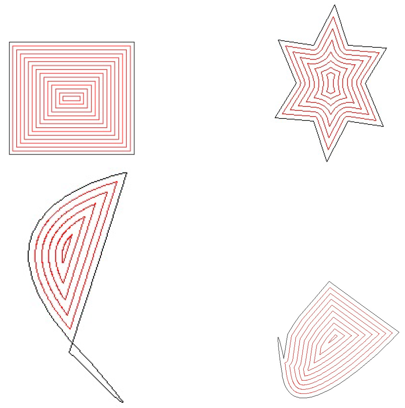
Article

Geometry-Aware Hatching Toolpath Selection and Parameter Optimization for Laser Marking of Complex Two-Dimensional Contours


1
School of Information Science and Engineering, Linyi University, Linyi 276000, China
2
School of Logistics, Linyi University, Linyi 276000, China
3
Department of Transportation Science, National Taiwan Ocean University, Keelung 202301, Taiwan
4
Department of Business Administration, Asia University, Taichung 413305, Taiwan
5
School of Software, Xi’an Jiaotong University, Xi’an 710049, China
*
Author to whom correspondence should be addressed.
Appl. Sci. 2026, 16(13), 6744; https://doi.org/10.3390/app16136744
Submission received: 13 May 2026 / Revised: 27 June 2026 / Accepted: 30 June 2026 / Published: 6 July 2026
(This article belongs to the Section Optics and Lasers)

Abstract

Laser marking of two-dimensional composite contours requires hatching paths that balance path length, computation time, coverage continuity, and marking accuracy. Existing industrial and academic systems commonly provide zigzag and contour-parallel hatching strategies, but the choice between them is often made empirically, especially for nested or irregular contours. This study is positioned as a geometry-aware toolpath-selection and parameter-optimization framework. Three benchmark contour types, namely a single-layer regular contour, a nested multi-layer contour, and an irregular contour, are evaluated using zigzag parallel hatching and contour-parallel hatching. The MATLAB results show that for the irregular benchmark contour, zigzag hatching reduces the toolpath-generation time by 73.91–89.62% compared with contour-parallel hatching when the hatch spacing varies from 0.01 to 0.10 mm. Five repeated numerical runs further show that the maximum relative timing deviation is below 0.003%, indicating stable computation in the software environment. To avoid confusing algorithmic computation time with real machine execution time, this paper explicitly separates toolpath-generation time from physical marking time and outlines a repeatable physical validation protocol including execution time, dimensional error, mark contrast, and line width uniformity. The results provide practical guidance for selecting hatching strategies according to contour complexity and accuracy requirements.

1. Introduction

Laser marking is a non-contact manufacturing process in which a focused laser beam modifies the surface of a target material to generate permanent text, graphics, codes, or functional marks. In modern marking systems, the optical and galvanometer components determine the physical capability of the machine, whereas the software-generated toolpath determines how the beam scans the designed contour. For complex two-dimensional graphics, the hatching path directly affects the total marked length, jump length, number of starts and stops, sharp turns, local over-marking, and final marking uniformity [1]. In related laser surface texturing and engraving studies, scanning strategy and process parameter selection has been shown to affect surface accuracy, texture quality, and productivity [2,3]. These findings indicate that hatching-path design should be considered as a geometry-dependent planning problem rather than as a purely graphical filling operation.
Among the most widely used filling strategies, zigzag or raster hatching scans the interior of a contour using approximately parallel lines, while contour-parallel hatching fills the region by inward offsets of the boundary. These two strategies are not new; they are common in laser-marking software, computer-aided manufacturing, and additive-manufacturing path planning. Previous studies have examined laser-marking path optimization using genetic algorithms, contour extraction, graphic hatching, and image-processing-based filling methods [4,5,6,7,8]. These works provide useful implementations for contour extraction and filling generation, but they give limited guidance on how the same pair of basic hatching strategies should be selected when the contour changes from regular to nested or irregular geometry. In additive manufacturing, path planning has likewise been shown to influence accuracy, surface quality, build time, and material use, and hybrid contour-zigzag paths have been proposed to improve continuity and filling performance [9,10]. This paper establishes a reproducible and interpretable framework for comparing the two basic strategies, zigzag hatching and contour-parallel hatching, for different contour geometries.
The practical problem addressed in this work is the following: given a two-dimensional contour with possible nested boundaries or irregular curvature, how can one select a suitable hatching strategy and hatch spacing so that the path-generation process is efficient while maintaining acceptable geometric coverage? If the contour is geometrically regular and has few holes or concave regions, zigzag hatching is expected to provide a shorter computation time and simpler path generation. If the contour is highly irregular, contains nested boundaries, or requires better boundary-following behavior, contour-parallel hatching may provide better geometric consistency but usually at the cost of a longer computation time and more offset operations.
To make this problem statement explicit, this paper distinguishes three different quantities: (i) toolpath-generation time, which is the MATLAB program running time needed to generate and evaluate the path; (ii) geometric path indicators, including total marking length, number of hatch lines or contour loops, and contour complexity; and (iii) machine execution time, which must be measured on a real laser-marking system and is affected by scanner acceleration, jump delay, laser power, pulse frequency, material properties, and controller settings. This distinction is essential because a short algorithmic running time does not automatically imply a shorter physical marking time.
The main contributions of this paper are summarized as follows:
1.
A geometry-aware comparison framework is established for zigzag parallel hatching and contour-parallel hatching over single-layer, nested multi-layer, and irregular two-dimensional contours.
2.
A shape complexity descriptor is introduced to support the distinction between regular and complex contours using compactness, hole number, concavity, and curvature variation.
3.
The roles of the Hough transform, curve fitting, and particle swarm optimization are clarified. In particular, Hough-based line fitting is treated as an optional raster-contour preprocessing step, while scanline-polygon intersection is recommended for vector contours.
4.
The numerical results are reported as toolpath-generation results rather than physical machine-processing results, and repeated runs are summarized using mean, standard deviation, maximum absolute deviation, and maximum relative deviation.
5.
A physical laser-marking validation protocol is outlined to support future experimental verification using real execution time, dimensional error, mark contrast, line width uniformity, and sample photographs.

2. Materials and Methods

2.1. Benchmark Contours and Hatching Task

For the single-layer contour, the zigzag and contour-parallel hatching procedures are evaluated by calculating the total hatching-curve length, the number of parallel lines or contour loops, and the program running time.
For single-layer contours, we do the following:
1: The discrete points in the first benchmark dataset are fitted into continuous smooth curves in MATLAB2022a, and the irregular single-layer contour is divided into several simpler blocks for subsequent hatching analysis.
2: Under the zigzag parallel hatching entity, the single-layer contour is made fractal by the zigzag function, the figure is processed into binary edge graphics, the set of coordinate points in the contour is extracted, and then the discrete points are fitted into straight lines by the combination of the Hough transform and least-square method [11] so as to calculate the length of the parallel lines. After the contour is made fractal, the height of each block is divided by the number of zigzag parallel lines.
3: Under contour-parallel hatching, representative discrete points are selected in each part of the contour. Each selected point is used as the center of a circle, and the inward offset distance is used as the radius. A smooth curve tangent to these circles is then constructed to obtain the nearest offset contour. The curve length is calculated using the first kind of curvilinear integral [12]. The multi-objective particle swarm optimization algorithm is then used to search for the deepest feasible contour layer, and the spacing between adjacent contour lines is used to estimate the number of contour loops.
4: The running times of two kinds of hatching entity programs are timed by clock function.
For contours with different shapes and hatch spacings, the two marking methods are tested under the same numerical framework. The goal is to compare their path-generation efficiency and geometric behavior under the following controlled conditions:
1: The hatching procedures are first evaluated on the single-layer and nested contours. An additional irregular contour composed of many discrete coordinates is then used to test whether the same procedures remain applicable to more complex geometry. The data obtained from the three contour types are compared to identify the relative advantages of zigzag parallel hatching and contour-parallel hatching.
2: The hatching procedure is then extended from regular straight-line contours to irregular curved contours, and the parameter results are used to observe how contour shape affects the algorithm. These results help identify the conditions under which either zigzag parallel hatching or contour-parallel hatching is more suitable.
3: The hatch spacing is varied in the interval [0.01, 0.1], and MATLAB is used to generate hatching paths for the fixed benchmark shapes so that the change in time T can be observed.
4: The optimization model is created by controlling the variables and using the obtained parameters to define a reference objective function f ( x ) for subsequent parameter analysis.

2.2. Toolpath Modeling and Optimization Framework

Interpolation curve modeling is used to obtain an approximate boundary function from a limited set of known data points [13]. Polynomial interpolation, including Lagrange interpolation and Newton interpolation, is used to approximate the contour curve. The optimal solution is obtained by establishing a mathematical model based on particle swarm optimization (PSO) [14]. The optimized parameters are used to calculate the number of parallel lines and contour loops. The crowding distance [15] is calculated and sorted to estimate the density of neighboring solutions around each candidate solution.
For each objective function, the solutions in the external optimal solution set are sorted by their objective values. The crowding distance is then calculated from the neighboring solutions, with the boundary solutions assigned an infinite crowding distance. A smaller crowding distance indicates a denser local distribution and lower diversity, whereas a larger crowding distance indicates a sparser local distribution and higher diversity. Finally, the particles are reordered according to the calculated crowding distance, and the global optimal value is selected from the group with a relatively large crowding distance [15].
i = 0.1 ( n o n d o m 1 ) , j = R a n d o m ( 0 , i ) , G b e s t = A [ j ]
Tips: The variable nondom is the number of non-inferior solutions, and A [ j ] is a random solution with a large crowding distance in the elite solution set. At this time, the randomly selected Gbest is an individual in the scattered region of the front end of the Pareto.

3. Experimental Design and Results

3.1. Software Environment and Scope of Numerical Evaluation

The numerical experiments were implemented in MATLAB and were used to evaluate software-level toolpath generation. The reported running time in the numerical sections is therefore the toolpath-generation time, not the real laser-marking execution time. The following assumptions are used in the software evaluation: (i) the input contour is represented by discrete coordinate points and can be reconstructed into a continuous boundary; (ii) the marked area can be divided into subregions suitable for scanline or contour-offset operations; (iii) the hatch spacing and inward offset distance are controllable geometric parameters; and (iv) material response, laser power, pulse frequency, scanner acceleration, and jump delay are excluded from the numerical timing model and must be evaluated separately in physical marking experiments.

3.2. Symbols and Definitions

For clarity and consistency, this section summarizes the principal symbols used throughout the proposed geometry-aware hatching-path selection and optimization framework, as shown in Table 1.

3.3. Shape Complexity Descriptor and Strategy Selection Criterion

To avoid an ambiguous distinction between “regular” and “complex” contours, a geometry-based descriptor is introduced. For a two-dimensional contour with area A and perimeter P, the compactness is defined as
K = P 2 4 π A .
For a circle, K = 1 , while elongated, concave, or highly irregular contours produce larger values. In addition, the number of internal holes H, the concavity ratio R c , and the curvature coefficient of variation C V κ are used to describe nested boundaries and local shape fluctuation. The composite contour-complexity score can be written as
S c = α K + β H + γ R c + δ C V κ ,
where α , β , γ , and δ are non-negative weights selected according to the application requirement. A lower S c indicates a more regular contour, for which zigzag hatching is usually efficient. A higher S c indicates a more complex contour, for which contour-parallel hatching or a hybrid strategy may be preferable if boundary-following accuracy is more important than computation time.
In the present numerical experiments, this descriptor is used as an explanatory criterion rather than as a trained classifier. It helps clarify why the same hatch spacing may lead to different relative advantages for single-layer, nested multi-layer, and irregular contours.

3.4. PSO-Based Parameter Optimization Objective

The particle swarm optimization component is used to optimize hatching-related parameters rather than to define the basic hatching strategies themselves. The design variables may include hatch spacing d, scanning angle θ , inward offset layer index k, and local connection order q. The general multi-objective cost function is formulated as
J ( d , θ , k , q ) = w 1 L m a r k + w 2 L j u m p + w 3 N s t a r t + w 4 C t u r n + w 5 E c o v e r ,
where L m a r k is the marking length, L j u m p is the non-marking jump length, N s t a r t is the number of laser on/off starts, C t u r n penalizes sharp turns, and E c o v e r measures uncovered and over-covered regions. The weights w 1 w 5 determine the relative importance of efficiency, path continuity, and coverage quality.

3.5. Benchmark Contour Description

To reconstruct the object boundary as accurately as possible, high-precision floating-point coordinate points are used as the benchmark contour data. These scattered points are fitted into smooth curves in MATLAB before hatching-path generation.
The Hough transform is used only when the input boundary is obtained from a raster image and near-straight segments must be detected before length calculation. For vector CAD or polygonal contour input, direct scanline-polygon intersection is a more direct and reproducible solution because it avoids unnecessary raster-to-line fitting. Similarly, global Lagrange interpolation is sensitive to oscillation when many nodes are used. Therefore, Lagrange interpolation is retained only as a local interpolation model in this paper, while piecewise cubic splines, B-splines, and NURBS are recommended for dense contour reconstruction in practical software implementations.
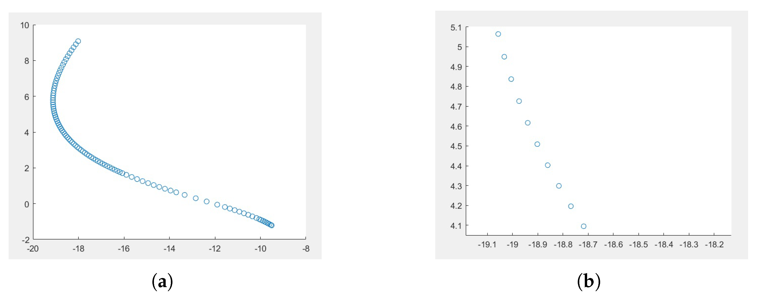
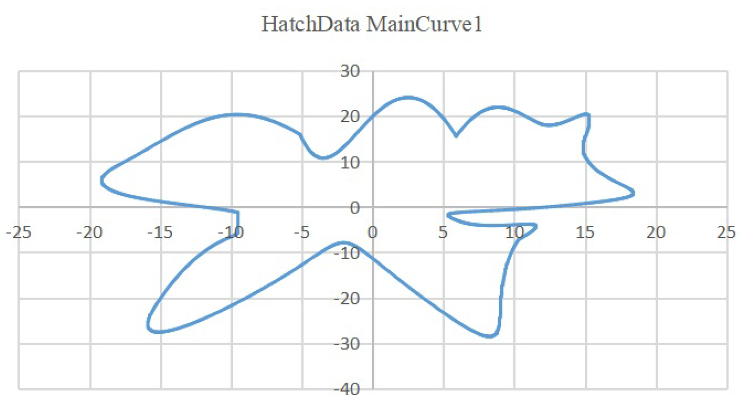
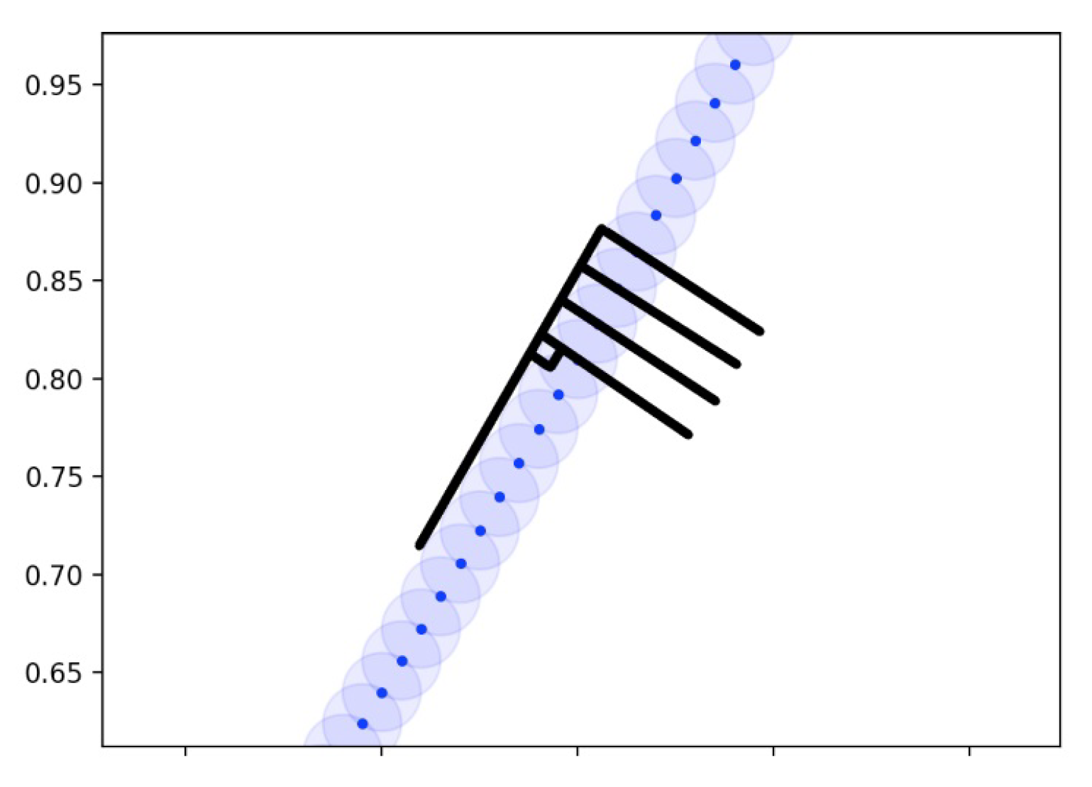
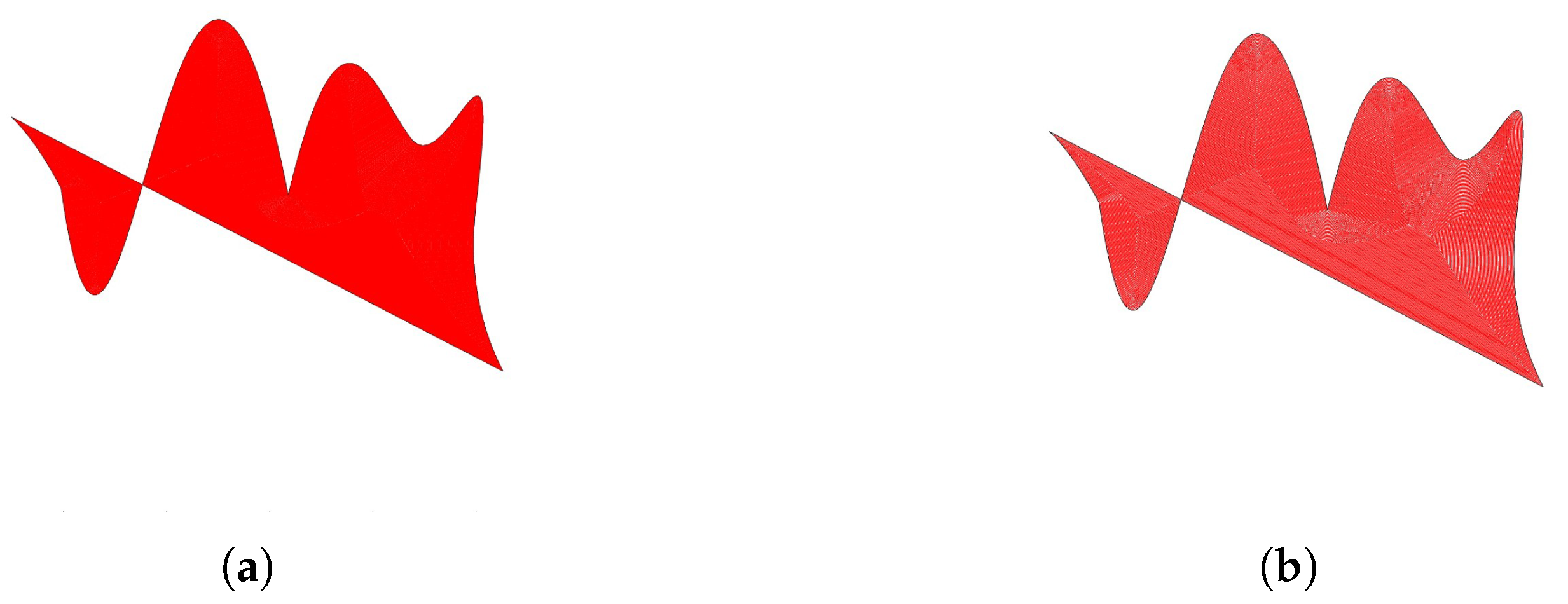
We select 100 data points from the data taken (as shown in Figure 1a), enlarge the graph, and show a scatter distribution (as shown in Figure 1b).

3.6. Hatching Path Generation Procedures

3.6.1. Single-Layer Contours

Firstly, the hatching model of the zigzag parallel hatch is established as follows:
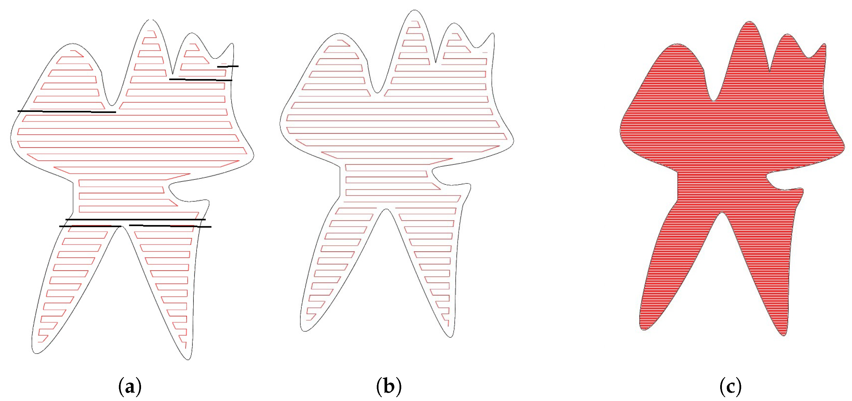
In order to obtain the length and number of parallel lines and contours of zigzag and contour lines, as well as the number of contour coils in single-layer contours under hypothetical conditions, the data given by us should be processed into smooth curves by MATLAB, and the Zigzag index algorithm model is established to fractalize the single-layer contours (Figure 2).
Solution of hatch model of zigzag parallel lines:
When using the zigzag parallel line method, calculate the height of each figure—the height divided by the hatch spacing is the number of horizontal lines in the broken-line parallel line—and extract the set of data points in the binary graph. The length of the zigzag parallel line is calculated by combining the Hough transform and the least-square method to fit the coordinates into a straight line [11].
According to the data given by us, we can get the single-layer contour. Let the set of coordinate points in the profile be M = ( x i , y i ) T , ( i = 1 , 2 , , s ) (s is the number of data points in the dataset), The data points in M are distributed near R lines, and the error threshold is set to d k . Under the standard parameterization mode, the expression of the straight line of the Hough transform in the plane’s Cartesian coordinate system is
ρ = x cos ϑ + y sin ϑ ; ρ 0 , 0 ϑ 2 π ;
Rewrite Formula ( 1 ) as follows:
ρ k = x i cos ϑ k + y i sin ϑ k ; ( i = 1 , 2 , , s ; k = 1 , 2 , r ) ;
According to Formula (2), M is transformed by the Hough transform, and the parameters of the fitting line can be obtained as follows: ( υ k , ρ k ) .
Record the set of points near the fitting line as M k * . Rewrite Formula ( 2 ) in its slope intercept form as follows:
y i = a k x i + b k
of which a k = cos ϑ k sin ϑ k , b k = ρ k sin ϑ k ;
Calculate the distance from a point in M to a straight line as follows:
d k i = | a k x i + b k y i | a k 2 + 1 x i , y i M , i = 1 , 2 , , s ; k = 1 , 2 , , R ;
If d k i < d k ,
then ( x i , y i ) M k * ( x k j , y k j ) , ( j = 1 , 2 , , s * , s * < = s ) .
M k * is the set of points near the line of the K t h * Hough transform that meets the requirement of the error threshold.
Taking the point set M k * as the fitting data, fitting each straight line, respectively, the parameters of the straight line Equation (8) can be obtained ( a k * , b k * ) . Choose ( ( x k j ) m i n , y k j ) M k * and ( ( x k j ) m a x , y k j ) M k * as endpoints, so the interval of each straight-line segment can be determined as follows:
y k j = a k * x k j + b k * , x k j min x k j x k j max .
Enter the data and get the following results:
Internal contraction of boundary distance of 1 mm and hatch line spacing of 1 mm:
length of hatching lines: 196.4336 mm; number of hatching horizontal lines: 85.
Internal contraction of boundary distance of 0.1 mm and hatch line spacing of 0.1 mm:
length of hatching lines: 989.5264 mm; number of hatching horizontal lines: 908.
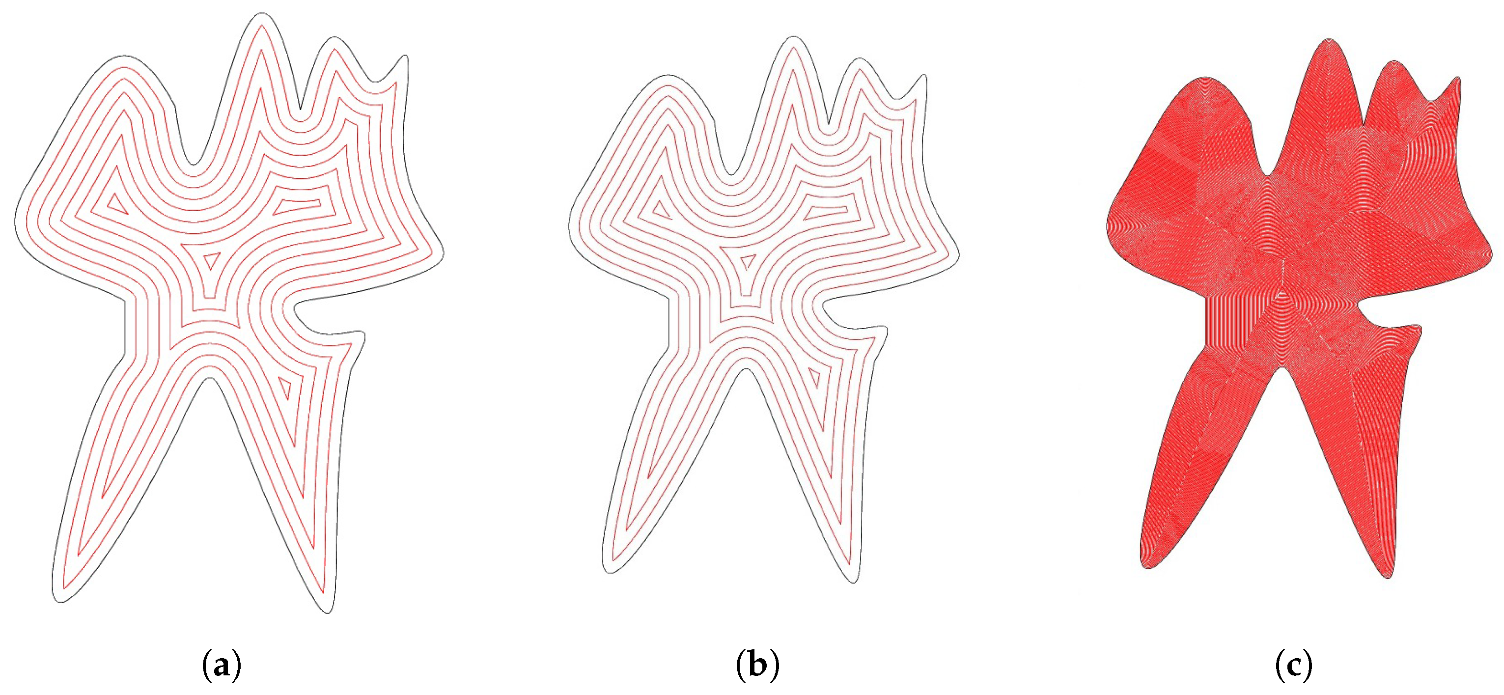
Establishment and solution of model of contour-parallel hatch (Figure 3a). The hatching model of contour-parallel hatches is established as follows:
The outline is reconstructed using a smooth curve fitted from the discrete-point parameters, as shown in (Figure 4).
Select some discrete points, take the discrete points as the center of the circle, take the internal indentation distance as the radius, specify the circle center, use a smooth curve to draw the tangent to each circle, obtain the tangent point, and use the algorithm to divide the curve into various parts. Find out the function of each part, and this smooth curve is the contour line closest to the contour, as shown in (Figure 5).
The existing curve function is used to approximately replace the contours. Solution of the contour-parallel hatching model.
The curve is fitted using the newly generated tangent points. Because the curve must pass through these points, the Lagrange interpolation polynomial is used to obtain an approximate curve function and construct a set of basis functions [16].
l i ( x ) = ( x x 0 ) ( x x i 1 ) ( x x i + 1 ) ( x x n ) ( x i x 0 ) ( x i x i 1 ) ( x i x i + 1 ) ( x i x n ) = j = 0 j i n x x j x i x j , ( i = 0 , 1 , n )
l i ( x ) is a polynomial of degree n, which satisfies
l i x j = 0 j i 1 j = i
Let
L n ( x ) = i = 0 n y i l i ( x ) = i = 0 n y i j = 0 j i n x x j x i x j
In the selected interval [ a , b ] , find a polynomial of degree n at most from the function values y i = f ( x i ) ( i = 0 , 1 , n ) at n + 1 different points x 0 , x 1 , , x n :
φ n ( x ) = a 0 + a 1 x + + a n x n
Make it have the same value as f ( x ) at a given point, that is, it satisfies the following interpolation condition:
φ n ( x i ) = f ( x i ) = y i ( i = 0 , 1 , n )
φ n is called an interpolation polynomial.
x i ( i = 0 , 1 , n ) is called an interpolation node. Make a polynomial curve y = f ( x ) . The N-degree polynomial ( 1 ) has n + 1 undetermined coefficient, and the interpolation condition ( 2 ) gives exactly an n + 1 equation.
a 0 + a 1 x 0 n + + a n x 0 n = y 0 a 0 + a 1 x 1 n + + a n x 1 n = y 1 a 0 + a 1 x n n + + a n x n n = y n
If the coefficient matrix of this system of equations is A, then
det ( A ) = 1 x 0 n 1 x n n
When the x 0 , x 1 , , x n values are different from each other, the value of this determinant is not zero. Therefore, the system of Equation ( 3 ) has a unique solution. Get the corresponding functional f ( x ) .
By introducing the obtained functional f ( x ) into the first kind of curve integral formula [12], the selected part of the contour length can be obtained as follows:
L f ( x , y ) d s = lim λ i = 1 n f ( ξ i , η i ) Δ s i
The curve length d 1 of the selected part can be obtained according to the selected interval [ a , b ] , and the curve function can be obtained from the difference curve.
In the process of creating the model, the discrete points are divided into n (n (countable constant) segment curves according to monotonicity, inflection points, extreme points, special points, etc.), the length d of each curve is obtained, and the following bus lengths can be obtained by adding the lengths of each segment:
C c = i = 1 n C 1 + C 2 + C n
The data given in Table 2 are modeled and solved, and the integrated shape does not need to be divided into regions. The contours are drawn and the algorithm is used to solve the value range of the bus length x. The value range of y is [ 19.12163645 , 18.4209696 ] . The value range of y is [ 28.53424723 , 24.06724352 ] .
Enter the data and get the following result:
Internal contraction of boundary distance of 1 mm and hatch line spacing of 1 mm:
Length of hatching lines: 896.8205 mm.
Internal contraction of boundary distance of 0.1 mm and hatch line spacing of 0.1 mm:
Length of hatching lines: 10,017.094 mm.
When hatching using the method of parallel contours, the multi-objective particle swarm optimization algorithm is used to find the optimal solution, that is, the deepest part of the contours, and the distance between the optimal solution and the farthest contour is calculated. The number of loops of the contours can be obtained by dividing the distance by the distance.
Obtained from the formula of the particle swarm optimization algorithm, the formula for determining the speed and position of particles in the search space is
ν t + 1 = ω ν t + c 1 · r ( ) · P b e s t x t + c 2 · r ( ) · G b e s t x t ;
x t + 1 = x t + ν t + 1
where ω is the inertia weight coefficient.
The best position of the particle itself and the global best position are P b e s t and G b e s t of the t generation, respectively. c 1 and c 2 are acceleration constants. r ( ) is a random number with a uniform distribution on [ 0 , 1 ] [17].
The formula after maintaining the inertia weight factor and acceleration factor is
v ( t + 1 ) = k [ ω v ( t ) + c 1 · r ( ) · ( P b e s t x ( t ) ) + ω v ( t ) + c 2 · r ( ) · ( G b e s t x ( t ) ) ]
where k 0.7 , 1.0 (k is a random number in [ 0.7 , 1.0 ] ).
So, we get the following result:
Internal contraction of boundary distance of 1 mm and hatch line spacing of 1 mm:
Length of hatching lines: 896.8205 mm; Number of hatching circles: 8.
Internal contraction of boundary distance of 0.1 mm and hatch line spacing of 0.1 mm:
Length of hatching lines: 10,017.094 mm; Number of hatching circles: 85.

3.6.2. Nested Multi-Layer Contours

Firstly, the hatching model of the zigzag parallel hatch is established as follows:
In order to obtain the length, the number of parallel lines, and the number of contour coils of the zigzag parallel lines and contours in the multi-layer test, the following must be conducted.
Considering the contours under hypothetical conditions, the data should be processed into smooth curves by MATLAB, and the nested contours should be separated using the zigzag index algorithm model.
The separated single-layer zigzag parallel (Figure 6a) solves the problem by using the method in Section 3.6.1 namely the establishment of parallel hatching model of nested multi-layer contour zigzag parallel.
The solution to the hatching model of the nested zigzag parallel lines is as follows:
When using zigzag parallel lines to hatch entities, the nested contours are separated first, and the height divided by the hatch spacing is the number of horizontal lines comprising the broken parallel lines. The set of data points in the binary graph is thus extracted. The length of the zigzag parallel line is calculated by combining the Hough transform and the least-square method to fit the coordinates into a straight line.
According to the given data, the nested profile can be obtained. After the contour is separated, the set of coordinate points in the contour is set to M = x i , y i T , i = 1 , 2 , , s , ( s is the number of data points in a dataset). The data points in M are distributed near R lines, and the error threshold is set to d k .
Taking the point set d k * as the fitting data, fitting each straight line, respectively, the parameters of the straight line Equation (3) can be obtained as ( a k * , b k * ) [16]. Choose ( ( x k j ) min , y k j ) M k * and x k j max , y k j M k * as endpoints. The interval of each straight line segment can be determined, that is,
y k j = a k * x k j + b k * , x k j min x k j x k j max .
The results can be obtained according to the models and formulas in the single-layer profile as follows:
Internal contraction of boundary distance of 1 mm and hatch line spacing of 1 mm:
Length of hatching lines: 189.0599 mm; number of hatching horizontal lines: 50.
Internal contraction of boundary distance of 0.1 mm and hatch line spacing of 0.1 mm:
Length of hatching lines: 1306.2959 mm; number of hatching horizontal lines: 525.
The entity of the contour-parallel hatch line is shown in Figure 7a. This figure shows the establishment and solution of the model of the contour-parallel hatch with a nested contour:
Solution of hatched entities with nested contours:
By separating the nested contour model [18] then using the same problem method, one can get the following results:
Internal contraction of boundary distance of 1 mm and hatch line spacing of 1 mm:
Length of hatching lines: 773.0452 mm; number of hatching circles: 5.
Internal contraction of boundary distance of 0.1 mm and hatch line spacing of 0.1 mm:
Length of hatching lines: 9060.1234 mm; number of hatching circles: 59.

3.6.3. Irregular Contours

For different shapes of graphics, different hatch spacings and different marking methods are tested.
In the process of laser marking, the time of task execution [19], the number of paths, and the distance of laser movement are different according to the size of the hatch line spacing, the shape of the polygon, and the type of marking. However, the production of these different results will lead to differences in work efficiency in practical applications. Treat the external indentation margin d, hatch spacing l, shape of the polygon x, hatching line type y, time T, path number N, and laser moving distance C as the dependent variables [19].
In order to meet the needs of the actual industry, a standard is established so that the time T is relatively short, the number of paths N is relatively small, and the laser moving distance C is relatively short. Using the optimization algorithm to create a mathematical model [20], on the basis of the original given data, this paper obtains several groups of data by adding new contours and constantly changing the spacing. Based on a large number of data, a set of criteria can be obtained, which can face different contours and carry out the most simple and efficient marking.
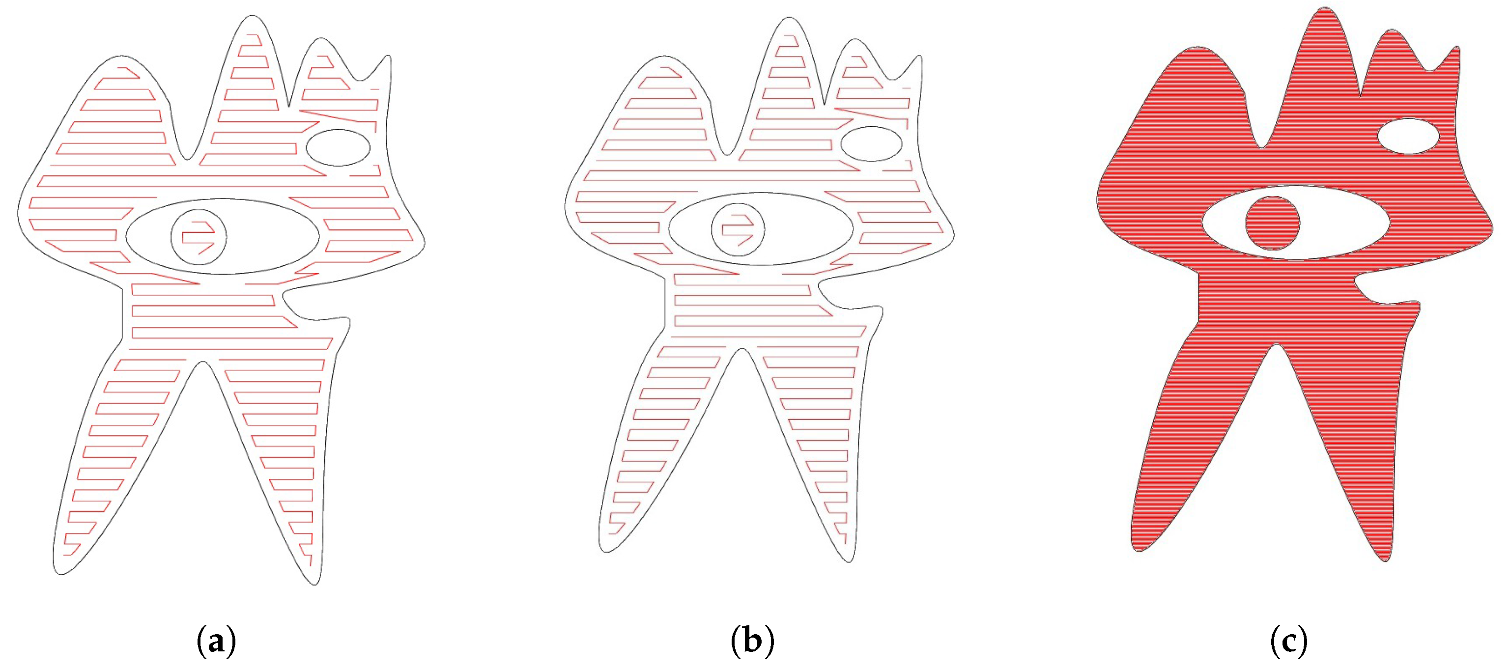
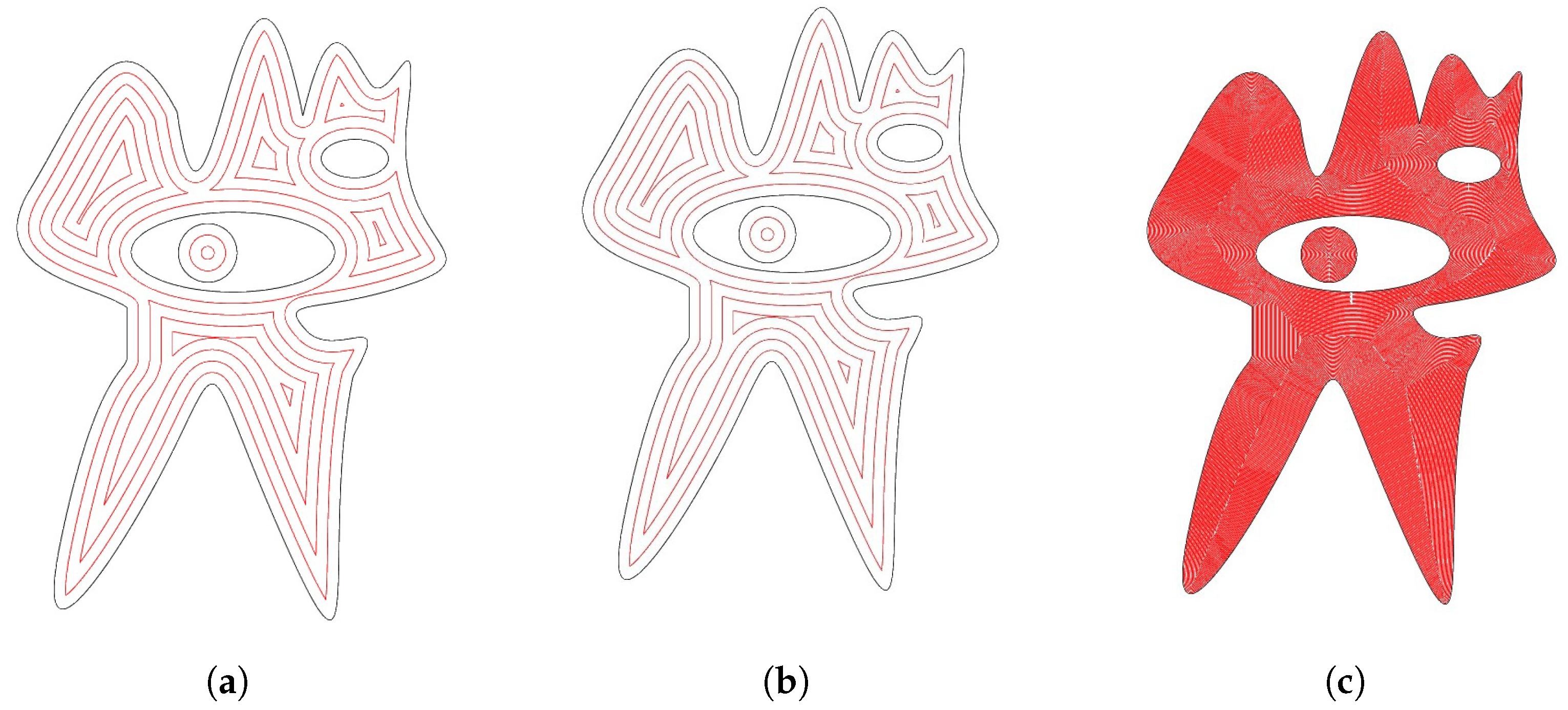
Next, we will deal with the contours of irregular polygons and analyze the data, as shown Figure 8.
The optimization model algorithm is applied to make the design index reach the optimal value.
For a set of variables that can be represented by a column vector X,
X = x 1 , x 2 , , x n T s . t . g i ( X ) 0 ( i , 1 , 2 , , n ) h j ( X ) = 0 ( j = 1 , 2 , , n ) max   f ( x ) o r min   f ( x )
Tips: s . t . is the abbreviation of “subject to”, which means “under the constraints of”.
m a x   f ( x ) means that the objective function takes the maximum value.
m i n   f ( x ) means that the objective function takes the minimum value.
f ( x ) is called the objective function. It is a real-valued continuous function of the design variable vector, and it is usually assumed to have a second-order continuous partial derivative. The objective function is the basis for comparing many design schemes that can be selected, and it is optimized to take the extreme value.
Deductive reasoning divides all contours into classified planning categories, which are divided into single-layer and nesting, and then the single-layer is divided into straight-line edge graphics, multilateral graphics, and curve graphics, which are continuously promoted from general to special, so as to ensure the accuracy of the data and a wide range of coverage.
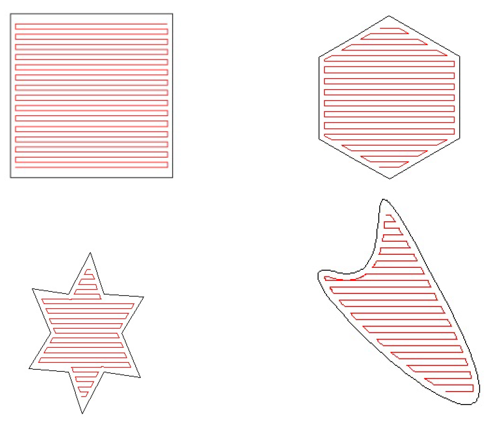
Select quadrilateral rectangles, hexagons, and twelve deformations and curves, and use MATLAB tools to hatch and fill zigzag parallel lines and contour-parallel lines, respectively [21]. Organize the image, verify the use of the function f ( x ) , and observe the results of f ( x ) and its feasibility.
Hatching filling curves of zigzag parallel lines with different shapes, as shown in Figure 9.
Select quadrilateral rectangles, along with twelve deformations and different curve shapes, and hatch and fill them with the algorithm program we have written.
Fill zigzag parallel hatching and parallel lines of contours, respectively [22]. Organize the image, verify the use of the function f ( x ) , and observe the results of f ( x ) and its feasibility, as shown in Figure 10.

3.7. Toolpath Visualization and Numerical Results

3.7.1. Bezier Curve Method

The Bezier curve is a general vector graphics software through which a curve can be drawn accurately. The Bezier curve is composed of line segments and nodes that contain draggable fulcrums and whose line segments are like retractable belts. It is a smooth curve drawn according to the coordinates of arbitrary points in four positions, and the pen tool we see on the drawing tool is used to create this kind of vector curve. The algorithms for calculating the length of a Bezier curve are mainly the particle swarm optimization algorithm and pattern search method [23]. The particle swarm optimization algorithm has the characteristics of being easy to understand and easy to implement, as well as having a strong global search ability, so it has attracted wide attention in the fields of science and engineering. The main purpose of the pattern search method is to extract the objective function from a direction set, find out the descending direction by comparing the value of the function, and then solve the problem. Because the Bezier curve is drawn according to the point coordinates of four positions, it is relatively easy to draw, but the error in calculating the length will be larger. In addition, when we selected the dataset, we chose a scattered point profile; the characteristics of the data also cause the error when calculating the length to be larger [24].

3.7.2. MATLAB Fitting Curve

If the MATLAB tool is used to fit the scatter profile into a smooth closed curve, when calculating the length of the zigzag parallel WEDM, the Hough transform and the least-square method are used to calculate the curve length. Using this method to calculate the length of zigzag parallel lines can reduce the error, improve the accuracy, and render it easy to control the effectiveness of the curves.
In the length calculation of the marking mode of the contour-parallel hatch, some discrete points are selected, the discrete points are taken as the center of the circle, the internal indentation distance is taken as the radius, the center of the circle is specified, and a smooth curve is tangent to each circle to obtain the tangent point. The curve is divided into parts by the algorithm, and the function of each part is obtained. This smooth curve is the nearest contour to the outline [25]. The curve can be fitted according to the new discrete point (tangent point). The curve must pass through the newly generated discrete points, and then the Lagrangian interpolation polynomial in the difference algorithm is used to obtain the approximate function of the curve to construct a set of basis functions. The final length can be calculated by using the first kind of curve integral. Using this method to calculate the length of parallel contours can minimize the error. When fitting the function, the structure of the formula is compact and easier to study.
Through analysis and comparison, our team, after a long period of consideration and experimentation because of the large error of the Bezier curve, finally chose to use the MATLAB fitting curve to present the experimental results. Although the calculation is more troublesome, the accuracy is very high.

3.7.3. Experimental Results

This section reports the numerical and physical validation results, focusing on toolpath-generation time, real machine execution time, dimensional accuracy, marking contrast, and line-width uniformity for different hatching strategies, as shown in Table 3.
The difference in time between the two hatching methods under the same outline can be clearly observed from the above table. Through the analysis, we get the specific fault-tolerance range of the two cutting methods, as well as the toolpath-generation time and the applicable profile. The following table (Table 4) shows an advantage table.
According to the advantage table (Table 4), the specific problems in real life can be analyzed, the parameters can be substituted into the optimization model, and the best scheme can be obtained to improve the efficiency and way of work.
Under the given constraint conditions and the condition of small errors, the given parameters can be accurately analyzed, and results close to those in real life can be obtained by using the laser printing software standard to draw the outline; the reference standard of how the parameters can be changed to improve the work efficiency should be used in laser marking [26].
Controllable range of error analysis of 0.001 < x < 0.01 : Use contour parallel;
Controllable range of error analysis of x < 0.001 : Use zigzag parallel;
Hope to spend less time: Use zigzag parallel;
There is not much demand for time: Use contour parallel;
The shape is similar to the regular figure: Use zigzag parallel;
The shape is similar to the irregular figure: Use contour parallel.
The above optimization algorithm rules are for reference.

3.8. Performance and Uncertainty Analysis

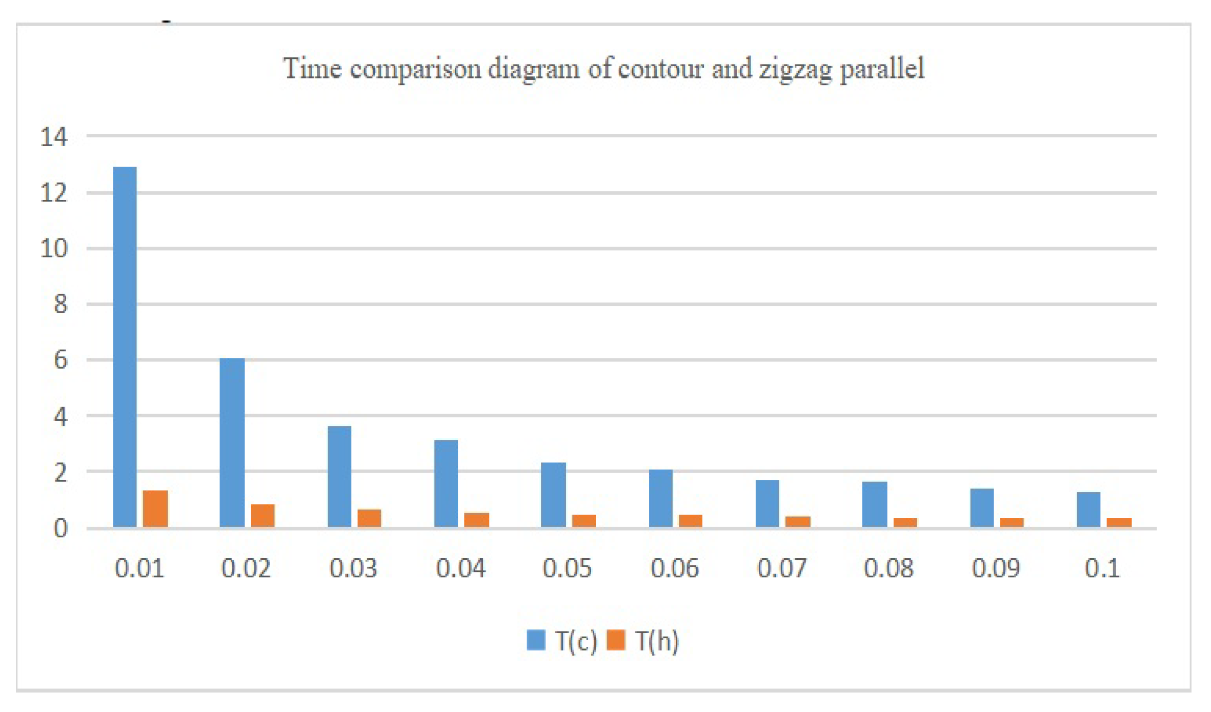
By using contour-parallel hatching and zigzag parallel hatching to deal with irregular contours, 10 groups of different interval data are selected and processed, respectively, and the results are as follows (Table 5).
In order to make it easier for us to observe, we made a histogram. Through further analysis and comparison, it can be seen intuitively that the hatching time of using zigzag parallel hatches in the selected irregular contours is less than that of using contour-parallel hatches, as shown in Figure 11.
For the irregular benchmark contour in Table 5, zigzag hatching reduces the MATLAB toolpath-generation time by 73.91–89.62% compared with contour-parallel hatching over hatch spacings from 0.01 to 0.10 mm. Table 6, Table 7 and Table 8 further show that the repeated MATLAB computations are numerically stable, with a maximum relative timing deviation below 0.003%. These values quantify software-level repeatability only; they do not replace real laser-marking execution time measurements.
As can be seen from the above table (Table 6 and Table 7), the smaller the distance between the hatches, the longer the time taken. This means that the denser the path of laser marking, the longer it takes. According to the data in the table, the outline of the object and the way it is marked by the laser will have an impact on time. For the same figure, the time gap between the two hatching methods is relatively large, so it is concluded that different hatching methods used by different graphics have their own characteristics, and different hatching methods need to be used for different graphics and hatch spacings.

3.9. External Baseline and Visual Comparison Protocol

To make the comparison more relevant to engineering practice, this paper should include at least one external baseline, such as the default hatch output from industrial laser-marking software or a reproducible scanline-polygon-filling algorithm. The baseline should be evaluated using the same contour set, hatch spacing, and measurement indicators. If a commercial software baseline is used, the software name, version, hatch mode, scanner settings, and export format should be reported, as shown in Table 9.
In addition to the numerical table, a complete visual comparison should include the generated paths and real marked samples. For each contour type, the recommended layout is as follows: original contour, zigzag path, contour-parallel path, external baseline path, and physical marking photograph. This figure is necessary because path length and MATLAB running time alone cannot fully demonstrate marking quality.

3.10. Physical Marking Validation Protocol and Data Reporting

Because the numerical evaluation alone cannot determine real marking quality, a physical laser-marking validation protocol is included. The minimum recommended validation is a full-factorial experiment with three contour types, two hatching strategies, two hatch spacings, and five repeated markings for each condition, resulting in 60 marked samples in total. The three contour types are regular contours, nested multi-layer contours, and irregular contours. The two hatching strategies are zigzag parallel hatching and contour-parallel hatching. The hatch spacings should be set according to the actual marking setup used in the experiment; in this paper, they are denoted as 0.10 mm and 0.20 mm and can be replaced by the values used in the laser control software.
For each marked sample, the real machine execution time T e should be recorded directly from the laser-marking control software. Dimensional error should be measured by comparing the marked boundary with the designed contour. Mark contrast can be calculated from the mean gray values of the marked region I m and the unmarked background I b as
C m = | I b I m | I b .
Line width uniformity should be reported using the coefficient of variation
C V w = σ w μ w × 100 % ,
where μ w and σ w are the mean and standard deviation of repeated line width measurements. Each condition should be repeated five times and reported as mean ± standard deviation. Representative photographs of the marked samples should be provided in the figure set to visually compare edge fidelity, fill uniformity, and local defects.
The physical validation is intended to separate algorithm computation time from real machine execution time. In the numerical experiments, the reported time corresponds to the MATLAB program running time, whereas in laser-marking practice, the final execution time is additionally affected by scanning acceleration, jump delay, laser power, pulse frequency, material response, and fill spacing, as shown in Table 10. Therefore, the measured T e should be discussed together with dimensional accuracy and mark quality indicators rather than being interpreted only as computational speed, as shown in Table 11.

4. Conclusions

First of all, for the single-layer profile and hatch with the zigzag parallel and contour-parallel hatches, we calculated the total length of the hatching curve and the number of parallel lines, the number of circles of contours, and the running time of the program. Zigzag parallel hatching and contour-parallel hatching were evaluated on single-layer, nested multi-layer, and irregular benchmark contours. The numerical results show that the preferred hatching strategy depends strongly on contour geometry and hatch spacing. For the irregular benchmark contour, zigzag hatching reduced the MATLAB toolpath-generation time by 73.91–89.62% compared with contour-parallel hatching when the hatch spacing varied from 0.01 to 0.10 mm. Repeated MATLAB runs showed a maximum relative timing deviation below 0.003%, indicating stable software-level computation.
This paper also clarifies an important limitation of the numerical study: the reported MATLAB running time is in toolpath-generation time, not real machine execution time. Real laser marking is additionally affected by scanner acceleration, laser on/off delay, jump motion, material response, laser power, pulse frequency, and the controller. Therefore, physical validation is required before making strong claims about real production efficiency. For this reason, a full-factorial validation protocol is provided, including three contour types, two hatching strategies, two hatch spacings, and five repeated markings per condition. The recommended physical indicators are real execution time, dimensional error, mark contrast, line width uniformity, and representative marking photographs.
The practical conclusion is that zigzag hatching is suitable for relatively regular contours when rapid toolpath generation is the priority, while contour-parallel hatching is more appropriate for nested or highly irregular contours when boundary-following consistency is more important. Future work should focus on completing physical marking experiments, adding external industrial software baselines, and further developing hybrid contour–zigzag paths for contours with mixed regular and irregular regions.

Author Contributions

Conceptualization: Z.X. and Y.C.; Data curation: Z.X. and J.Y.; Formal analysis: Z.X. and J.Y.; Funding acquisition: Y.C.; Investigation: Z.X.; Methodology: Z.X.; Project administration: Y.C.; Resources: Y.C.; Software: Z.X. and J.Y.; Supervision: Y.C.; Validation: Z.X., Y.C., and J.-C.W.; Visualization: Z.X.; Writing—original draft: Z.X.; Writing—review and editing: Y.C. and J.-C.W. All authors have read and agreed to the published version of the manuscript.

Funding

This study was funded by the Major Science and Technology Innovation Project of the key RD plan of Shandong Province, Project No.: 2019jzy010134, theory and key technology of large industrial equipment network management and control security.

Institutional Review Board Statement

Not applicable.

Informed Consent Statement

Not applicable.

Data Availability Statement

The raw data supporting the conclusions of this article will be made available by the authors on request.

Conflicts of Interest

The authors have no conflicts of interest to declare that are relevant to the content of this article.

References

  1. Moskal, D.; Martan, J.; Honner, M. Scanning Strategies in Laser Surface Texturing: A Review. Micromachines 2023, 14, 1241. [Google Scholar] [CrossRef] [PubMed]
  2. Martan, J.; Moskal, D.; Honner, M. Performance and Accuracy of the Shifted Laser Surface Texturing Method. Micromachines 2020, 11, 520. [Google Scholar] [CrossRef]
  3. Dondieu, S.D.; Wlodarczyk, K.L.; Harrison, P.; Hand, D.P. Process Optimization for 100 W Nanosecond Pulsed Fiber Laser Engraving of 316 L Grade Stainless Steel. J. Manuf. Mater. Process. 2020, 4, 110. [Google Scholar] [CrossRef]
  4. Wang, D.; Yu, Q.; Zhang, Y. Research on Laser Marking Speed Optimization by Using Genetic Algorithm. PLoS ONE 2015, 10, e0126141. [Google Scholar] [CrossRef] [PubMed]
  5. Wang, Z.; Bai, Y.; Luo, X. Creation and Optimization of Laser Marking Hatch Contour Generation Algorithm. In Proceedings of the 2021 International Conference on Information Technology, Education and Development (ICITED 2021); Francis Academic Press: London, UK, 2021; pp. 519–523. [Google Scholar] [CrossRef]
  6. Luo, X.; Wang, Z.; Bai, Y. Optimization Algorithm Design of Laser Marking Contour Extraction and Graphics Hatching Based on Image Processing Technology. J. Phys. Conf. Ser. 2022, 2173, 012078. [Google Scholar] [CrossRef]
  7. Luo, J.; Duan, C. Optimization Algorithm Design Based on Laser Marking Contour Extraction and Graphic Filling. In Proceedings of the 2025 IEEE 3rd International Conference on Image Processing and Computer Applications (ICIPCA); IEEE: Piscataway, NJ, USA, 2025; pp. 878–882. [Google Scholar] [CrossRef]
  8. Lu, G.; Liu, Y.; Yao, X.; Yang, J.; Jia, C. Exploration of Laser Marking Path and Algorithm Based on Intelligent Computing and Internet of Things. Comput. Intell. Neurosci. 2022, 2022, 7443410. [Google Scholar] [CrossRef] [PubMed]
  9. Jiang, J.; Ma, Y. Path Planning Strategies to Optimize Accuracy, Quality, Build Time and Material Use in Additive Manufacturing: A Review. Micromachines 2020, 11, 633. [Google Scholar] [CrossRef] [PubMed]
  10. Bi, M.; Xia, L.; Tran, P.; Li, Z.; Wan, Q.; Wang, L.; Shen, W.; Ma, G.; Xie, Y.M. Continuous Contour-Zigzag Hybrid Toolpath for Large Format Additive Manufacturing. Addit. Manuf. 2022, 55, 102822. [Google Scholar] [CrossRef]
  11. Zeng, J.-X.; Zhang, G.-M.; Chu, J.; Lu, Y.-M. Fit Line Using a Method Combined Hough Transform with Least Square. J. Nanchang Hangkong Univ. Nat. Sci. Ed. 2003, 17, 9–13. [Google Scholar]
  12. Jing, H.; Wang, Z. On Calculations of First Type Curvilinear Integrals; Department of Basic Courses, Rocket Force University of Engineering: Xi’an, China, 2020; Volume 23, pp. 16–19+36. [Google Scholar]
  13. Zhang, X.-Y.; Lei, Y.-F.; Liu, P.-P.; Bao, F.-X.; Zhang, Y.-F. Curve Modeling Using Rational Fractal Interpolation with Variable Parameters. J. Graph. 2021, 42, 245–255. [Google Scholar] [CrossRef]
  14. Yang, W.; Li, Q. Summary of Particle Swarm Optimization Algorithm. Eng. Sci. 2004, 6, 87–94. [Google Scholar]
  15. Wei, W.; Guo, Y. Dynamic Particle Swarm Algorithm for Multi-Objective Optimization Based on Crowding Distance. Comput. Eng. Des. 2011, 32, 1422–1425+145. [Google Scholar]
  16. Sheng, L.; Zeng, Z. Research on Curve Fitting Principle and Its Application. Master’s Thesis, Changsha University of Science and Technology, Changsha, China, 2015. [Google Scholar]
  17. Chen, M. Research on Improved Particle Swarm Optimization Algorithm for Optimization Problems. Master’s Thesis, Jilin University, Changchun, China, 2015. [Google Scholar]
  18. Li, M.; Zhang, L.-C.; Mo, J.-H.; Zhao, Z.-Y. Smoothing Technique for 2D Contour in Numerical Control Plasma Cutting. Comput. Integr. Manuf. Syst. 2011, 17, 2623–2628. [Google Scholar]
  19. Cao, R.; Qiu, H.; Li, J.; Wang, A.; Lu, C. Quality Assessment and Technical Parameter Optimization of Laser Direct Part Marking. Appl. Laser 2011, 31, 151–156. [Google Scholar] [CrossRef]
  20. Li, Y.; Zhang, B. Research on path optimization algorithm for Complex contour laser Cutting. J. Tianjin Univ. Technol. Eng. Version 2007, 23, 6–79. [Google Scholar]
  21. Tao, X.; Li, Z.; Wang, H. Optimal solution of matrix layout based on filling algorithm. China Mech. Eng. 2003, 14, 1104–1107. [Google Scholar]
  22. Shi, H.; Chen, X.; Lai, Z.; Ouyang, P.; Ou, L. Contour Line Drawing Based on Discrete Data. Chin. J. Eng. Geophys. 2006, 3, 484–487. [Google Scholar]
  23. Shen, Z.; Liu, X.; Fei, X.; Kang, K. Laser galvanometer processing algorithm based on point set Bezier curve optimization. Laser Technol. 2021, 45, 548–553. [Google Scholar]
  24. Yang, Y.; Wang, Y. Research and implementation of hand-drawn Line Vectorization Technology. Comput. Eng. Sci. 2011, 33, 128–131. [Google Scholar]
  25. Liu, b.; Huang, S. Optimization of laser marking noozzle path in layered solid manufacturing technology. J. Comput. Aided Des. Graph. 2004, 16, 660–665. [Google Scholar]
  26. Situ, J.-M.; Liu, Y.; Yan, M.-X.; Zhang, X.-Y. Research of a New Method for Marking Laser-Induced Gray Images. Laser Technol. 2010, 34, 389–391. [Google Scholar]
Figure 1. (a) The outline of the selected 100 points. (b) Enlarged data point.
Applsci 16 06744 g001
Figure 2. (a) Single-layer contour fractal analysis figure. (b) Internal contraction of boundary distance: 1 mm; hatch line spacing: 1 mm. (c) Internal contraction of boundary distance: 0.1 mm; hatch line spacing: 0.1 mm.
Applsci 16 06744 g002
Figure 3. (a) Single-layer contour fractal analysis diagram. (b) Internal contraction of boundary distance: 1 mm; hatch line spacing: 1 mm. (c) Internal contraction of boundary distance: 0.1 mm; hatch line spacing: 0.1 mm.
Applsci 16 06744 g003
Figure 4. Outline drawing.
Applsci 16 06744 g004
Figure 5. To find the tangent, each discrete point ( x , y ) is used to simulate circle 1.
Applsci 16 06744 g005
Figure 6. (a) Nested multi-layer contour analysis diagram. (b) Internal contraction of boundary distance: 1 mm; hatch line spacing: 1 mm. (c) Internal contraction of boundary distance: 0.1 mm; hatch line spacing: 0.1 mm.
Applsci 16 06744 g006
Figure 7. (a) Nested multi-layer contour analysis diagram. (b) Internal contraction of boundary distance: 1 mm; hatch line spacing: 1 mm. (c) Internal contraction of boundary distance: 0.1 mm; hatch line spacing: 0.1 mm.
Applsci 16 06744 g007
Figure 8. (a) Internal contraction of boundary distance: 1 mm; hatch line spacing: 1 mm. (b) Internal contraction of boundary distance: 0.1 mm; hatch line spacing: 0.1 mm.
Applsci 16 06744 g008
Figure 9. Hatching filling curves of zigzag parallel lines with different shapes.
Applsci 16 06744 g009
Figure 10. Hatching filling curves of contour-parallel lines with different shapes.
Applsci 16 06744 g010
Figure 11. Toolpath-generation time comparison between contour-parallel hatching and zigzag hatching for the irregular benchmark contour.
Applsci 16 06744 g011
Table 1. A table consisting of a number of representative discrete points used to solve the model.
SymbolsDefinitions
JLeast-square index of curve
T ( d ) The hatch spacing is D-round’s hatching time
C c The total length of contour
C h The total length of horizontal lines
IThe number of the drawing area
N c The number of contour
N h The total length of horizontal lines
Table 2. A table consisting of a number of representative discrete points used to solve the model.
Center of the Circle XCenter Ordinate YRadius R
15.661620.9740861
15.488540.9127931
15.309220.8508081
15.217200.8195461
15.032350.7576151
14.667240.6383571
14.308330.5250691
Table 3. Summary of numerical toolpath-generation results for single-layer and nested multi-layer benchmark contours. C c and C h denote total contour-parallel and zigzag hatching lengths, N c and N h denote the corresponding number of contour loops and zigzag hatch lines, and T ( c ) and T ( h ) denote MATLAB toolpath-generation time.
Single-Layer CurvesMulti-Layer Curves
Internal contraction
of boundary
distance/mm
10.110.1
Hatch line
spacing/mm
10.110.1
C c /mm896.8210,017.094773.04529060.1234
C h /mm196.4336989.5264189.05991306.32959
N c 885559
N h 8590850525
T ( c ) /ms709.625839606.6224088
T ( h ) /ms249.88600.2228.224780
T ( h ) / T ( c ) 0.35210.1030.292590.148
Table 4. Qualitative strategy-selection table derived from the numerical comparison. The table should be interpreted together with the contour-complexity descriptor and the required accuracy level.
Zigzag Parallel HatchContour-Parallel Hatch
High precision
(Error < 0.001 mm)
High precision
(Error in 0.001∼0.01 mm)
Short use timeLong use time
Suitable for regular graphicsStrong applicability
Table 5. Toolpath-generation time comparison between contour-parallel hatching and zigzag hatching for the same irregular benchmark contour when the hatch spacing varies from 0.01 to 0.10 mm.
Hatch Line SpacingTc(d)/sTh(d)/s
0.01 mm12.9294121.341666
0.02 mm6.087090.81583
0.03 mm3.6300820.644071
0.04 mm3.1442930.541725
0.05 mm2.3333830.460358
0.06 mm2.0807370.461272
0.07 mm1.6846170.377026
0.08 mm1.6385580.372791
0.09 mm1.4045930.356446
0.10 mm1.2776460.333292
Table 6. Repeated MATLAB toolpath-generation time for the single-layer contour. Five repeated runs were conducted for each hatching condition.
TypeTime1Time2Time3Time4Time5Avg
Single-layer
contour
T c ( 1 ) 0.7091530.7091830.7091660.709170.7091680.709168
T c ( 0.1 ) 5.8392715.8392725.8392795.8392615.8392875.839274
T h ( 1 ) 0.2498720.2498730.249880.2498770.2498750.249875
T h ( 0.1 ) 0.6002030.6002040.60020.6001990.6001950.600201
Table 7. Repeated MATLAB toolpath-generation time for the nested multi-layer contour. Five repeated runs were conducted for each hatching condition.
TypeTime1Time2Time3Time4Time5Avg
Multi-layer
contour
T c ( 1 ) 0.6066280.606620.6066210.606640.6066170.606622
T c ( 0.1 ) 4.0881264.0881264.0881254.0881274.0881264.088126
T h ( 1 ) 0.2282220.2282260.2282280.2282240.228220.228224
T h ( 0.1 ) 0.7799840.7799920.7799980.7799980.7800080.779996
Table 8. Repeatability statistics of the MATLAB toolpath-generation time. The maximum relative deviation is calculated as the maximum absolute deviation from the mean divided by the mean value.
ConditionMean (s)SD (s)Max. Abs. Dev. (s)Max. Rel. Dev. (%)
Single-layer T c ( 1 ) 0.7091680.0000110.0000150.0021
Single-layer T c ( 0.1 ) 5.8392740.0000100.0000130.0002
Single-layer T h ( 1 ) 0.2498750.0000030.0000050.0018
Single-layer T h ( 0.1 ) 0.6002010.0000040.0000060.0010
Nested T c ( 1 ) 0.6066250.0000090.0000150.0024
Nested T c ( 0.1 ) 4.0881260.0000010.0000010.0000
Nested T h ( 1 ) 0.2282240.0000030.0000040.0018
Nested T h ( 0.1 ) 0.7799960.0000090.0000120.0015
Table 9. External baseline comparison at hatch spacing d = 0.10 mm. T g denotes the toolpath-generation time rather than the real machine execution time. The baseline corresponds to a reproducible raster scanline hatching implementation and should be replaced by measured values from a validated external-baseline implementation.
ContourMethodd (mm) T g (s) L mark (mm) L jump (mm)Starts/Stops
RegularZigzag0.100.600989.52682.430908
RegularContour-parallel0.105.83910,017.094146.28085
RegularBaseline0.100.7421125.684238.510946
NestedZigzag0.100.7801306.330126.750525
NestedContour-parallel0.104.0889060.123194.63059
NestedBaseline0.100.9141498.270362.840584
IrregularZigzag0.100.333684.920158.740312
IrregularContour-parallel0.101.2783826.450221.53047
IrregularBaseline0.100.486812.360428.190365
Table 10. Laser-marking equipment and process parameters used for physical validation.
ItemValue
MaterialPolished SS304 plate
Laser sourcePulsed fiber laser, 1064 nm
Average power20 W
Pulse frequency/width50 kHz/100 ns
Scanning speed800 mm/s
F-theta lens/spot size160 mm/∼30 μ m
Hatch spacing0.10 mm, 0.20 mm
Galvo setting8000 mm/s2, 100 μ s jump delay
Repeated markings5 per condition
Imaging deviceDigital microscope, 2448 × 2048 pixels
Table 11. Physical laser-marking validation results under different contour types, hatching strategies, and hatch spacings. Each condition was repeated five times, and the results are reported as mean ± standard deviation.
Contour TypeStrategyd (mm) T e (s)Dim. Error (mm)ContrastLine-Width CV (%)
RegularZigzag0.10 9.620 ± 0.088 0.032 ± 0.004 0.659 ± 0.008 6.663 ± 0.563
RegularZigzag0.20 4.806 ± 0.180 0.040 ± 0.003 0.612 ± 0.013 7.659 ± 0.800
RegularContour-parallel0.10 11.125 ± 0.165 0.028 ± 0.004 0.650 ± 0.011 5.669 ± 0.442
RegularContour-parallel0.20 5.600 ± 0.089 0.033 ± 0.003 0.595 ± 0.014 6.651 ± 0.798
NestedZigzag0.10 12.630 ± 0.247 0.042 ± 0.003 0.652 ± 0.026 8.369 ± 0.628
NestedZigzag0.20 6.435 ± 0.230 0.065 ± 0.005 0.588 ± 0.017 9.042 ± 0.694
NestedContour-parallel0.10 16.656 ± 0.266 0.029 ± 0.004 0.662 ± 0.018 6.134 ± 0.461
NestedContour-parallel0.20 8.257 ± 0.124 0.045 ± 0.002 0.601 ± 0.020 7.388 ± 0.649
IrregularZigzag0.10 15.962 ± 0.458 0.064 ± 0.003 0.613 ± 0.014 11.455 ± 1.311
IrregularZigzag0.20 8.066 ± 0.085 0.086 ± 0.014 0.551 ± 0.025 12.611 ± 0.601
IrregularContour-parallel0.10 23.141 ± 0.988 0.040 ± 0.005 0.653 ± 0.025 7.076 ± 0.710
IrregularContour-parallel0.20 11.993 ± 0.326 0.053 ± 0.007 0.575 ± 0.019 8.029 ± 0.426
Disclaimer/Publisher’s Note: The statements, opinions and data contained in all publications are solely those of the individual author(s) and contributor(s) and not of MDPI and/or the editor(s). MDPI and/or the editor(s) disclaim responsibility for any injury to people or property resulting from any ideas, methods, instructions or products referred to in the content.