


Featured Application
The proposed framework can be applied in non-contractual retail and e-commerce settings to predict customer lifetime value under zero-inflated conditions, support marketing resource allocation through dual-dimension purchase-probability and spending–intensity segmentation, and provide interpretable feature-level insights via SHapley Additive exPlanations (SHAP) analysis to guide customer relationship management decisions.
Abstract
This study proposes a two-stage Hurdle machine-learning framework for Customer Lifetime Value (CLV) prediction under zero-inflated non-contractual retail settings, where conventional single-stage approaches may suffer from prediction instability and retransformation issues when zero and non-zero spending are jointly modeled. Using the UCI Online Retail II dataset, comprising 4026 customers with a 62.5% zero-spending rate, Stage 1 employs XGBoost to estimate purchase occurrence probability, while Stage 2 applies gradient- boosting regressors to predict conditional spending intensity. The inverse hyperbolic sine (arcsinh) transformation handles 59 customers with negative net spending from product returns. The Two-stage CatBoost model achieves a coefficient of determination of 0.522, outperforming the best single-stage mean-squared-error (MSE) model (0.385), the default Tweedie-loss baseline in the main 30-seed comparison (0.309), and the Beta-Geometric/Negative Binomial Distribution (BG/NBD) baseline (0.395). The contribution combines architectural innovation with a comprehensive validation protocol—including 5 × 2 CV paired t-tests, out-of-time validation, and SHAP interpretability—confirming that purchase frequency drives occurrence probability while monetary value dominates spending magnitude. A dual-dimension segmentation based on purchase probability (P) and conditional spending intensity (E) identifies 96 Dormant, High-E customers with only a 26% purchase rate despite high expected spending, demonstrating that high conditional spending does not guarantee purchase occurrence.
1. Introduction
With the expansion of digital commerce, firms increasingly use customer-level data to guide marketing and customer relationship management (CRM) decisions [1]. In CRM research, customer lifetime value (CLV) is conventionally defined as the discounted value of future profit attributable to an individual customer over their relationship with the firm. In practice, however, non-contractual retail settings frequently lack the cost, margin, and customer-lifetime data required for this strict formulation; consequently, machine-learning-based CLV research operationalizes CLV as expected future revenue within a fixed prediction window—a widely adopted approach for assessing customer assets and long-term firm value in retail analytics [2]. As CRM has moved beyond operational contact management toward strategic customer engagement and value creation, CLV prediction has become a central tool for customer-oriented decision making [3,4].
Retail and e-commerce transaction data often contain many zero outcomes and a highly skewed positive tail, creating difficulties for conventional prediction models. A common response is to transform the target variable, especially by using a logarithmic transformation. However, returning predictions from the transformed scale to the original monetary scale can introduce retransformation bias, a well-established issue in econometrics and health expenditure modeling [5,6]. In zero-inflated CLV data, this problem is further complicated because zero and non-zero spending observations may arise from different behavioral processes.
Machine-learning approaches have increasingly been applied to CLV prediction and customer segmentation [7,8,9]. Many of these studies, however, still rely on single-stage regression frameworks. In zero-inflated settings, the occurrence of a future purchase and the amount spent conditional on purchase are conceptually distinct processes. A single model that estimates both simultaneously may therefore mix two different statistical mechanisms, weakening prediction stability and interpretability.
Prior studies have addressed CLV prediction challenges through sequential architectures, enriched feature representations, or distributional modeling strategies [10,11,12]. These approaches are valuable, but they mainly operate through feature design or distributional assumptions. Less attention has been paid to whether zero-inflation should be handled directly at the model architecture level by separating purchase occurrence from conditional spending intensity.
Two-stage Hurdle models provide such an architectural separation. They decompose the outcome-generating process into an occurrence component and a positive-outcome intensity component, and have been applied to zero-inflated domains such as health care demand [13], precipitation forecasting [14], and zero-inflated insurance claims [15]. Extending this occurrence–intensity principle to non-contractual CLV prediction is therefore statistically motivated, especially when a short prediction window produces a large proportion of non-purchasing customers.
This study applies a two-stage Hurdle gradient-boosting framework to short-term CLV prediction. Stage 1 estimates purchase occurrence probability, whereas Stage 2 estimates conditional spending intensity among buyers. To isolate the architectural effect from feature engineering, the main experiment uses a parsimonious and interpretable RFM feature set. The contribution is not the Hurdle concept itself, but its integration with gradient-boosting models, controlled validation, high-value customer identification, P × E segmentation, and SHAP-based interpretation within a zero-inflated CLV setting.
The objectives of this study are threefold. First, we construct a two-stage CLV prediction framework based on gradient-boosting algorithms and compare it with single-stage alternatives. Second, we extend evaluation beyond regression accuracy by considering top-20% high-value customer identification and P × E dual-dimension segmentation. Third, we assess statistical reliability and temporal generalization through cross-algorithm comparison, 5 × 2 cross-validation paired t-tests, sign tests, out-of-time validation, and SHAP-based interpretation.
The contributions of this work are as follows. First, we provide empirical evidence of the difference between single-stage and two-stage architectures under zero-inflated CLV data, showing that occurrence–intensity decomposition can improve prediction stability relative to models that jointly estimate zero and non-zero spending. Second, we develop a validation protocol that combines 5 × 2 cross-validation paired t-tests, sign tests, and cross-year out-of-time validation. Third, we introduce a P × E segmentation view that separates purchase probability from conditional spending, allowing dormant, high-expected-spending customers to be identified as a distinct risk segment. Fourth, SHAP analysis reveals a complementary feature structure across the two stages: frequency dominates purchase occurrence, whereas monetary value dominates conditional spending intensity, a pattern consistent with established customer-base analysis theory.
2. Related Work
2.1. CLV Prediction Methods and Zero-Inflation
CLV prediction methods can be broadly discussed along three methodological streams. The first stream is based on RFM analysis, which uses recency, frequency, and monetary value to summarize customer behavior for segmentation and targeting [16]. The second stream is based on probabilistic customer-base models, such as Pareto/NBD and BG/NBD [17,18]. These models provide interpretable formulations of customer purchasing and dropout processes, although their distributional assumptions may be restrictive in highly heterogeneous e-commerce data.
The third stream consists of machine-learning and ensemble-based approaches, including tree-based methods such as XGBoost [19], LightGBM [20], and CatBoost [21]. Recent CLV studies have reported promising results using two-stage tree ensembles [8], personalized CLV systems [9], sequence-to-sequence models [10], and flexible machine-learning frameworks [22]. However, many such approaches still rely on single-stage prediction architectures, in which zero and non-zero spending are estimated within the same regression process. Under zero-inflated conditions, this may blur the distinction between purchase occurrence and spending intensity, leading to prediction instability and reduced interpretability.
Zero-inflated outcomes have long been studied in statistics and actuarial science. Hurdle and zero-inflated models explicitly distinguish between the occurrence process and the positive-outcome process [11,12,23]. Recent work has further combined interpretable machine learning with generalized Hurdle models in healthcare demand analysis [13], while gradient-boosting approaches have also been examined for zero-inflated insurance claims [15]. These studies support the relevance of occurrence–intensity decomposition for skewed and zero-heavy data. However, the architectural treatment of zero-inflation remains less fully examined in non-contractual CLV prediction.
2.2. CLV-Based High-Value Customer Identification
CLV has long been used to support customer value assessment, relationship management, and marketing resource allocation [24]. Nevertheless, aggregate regression metrics such as R2, MAE, and RMSE do not directly evaluate whether a model can identify high-value customers for targeting decisions. A model may achieve acceptable overall prediction error while still failing to distinguish the customers most relevant for marketing intervention.
Prior research has approached CLV modeling through two-stage ensemble prediction, customer-segment dynamics, and customer-base analysis [8,25,26]. In particular, customer-segment dynamics have been shown to provide useful information for CLV prediction [25]. However, many model-comparison studies still emphasize aggregate prediction error, leaving targeting-oriented evaluation less explicit. Therefore, this study complements regression metrics with a top-20% high-value customer identification task using Precision, Recall, and F1-score.
2.3. Research Gaps
This review is motivated by three research gaps. First, although zero-inflation has been examined through distributional models and related applications, there is still limited CLV evidence on architectures that explicitly separate purchase occurrence from conditional spending intensity. Second, existing CLV model comparisons often emphasize aggregate prediction accuracy, whereas high-value customer identification and segmentation-oriented evaluation remain less systematically examined. Third, validation protocols that jointly assess statistical significance, directional consistency, and temporal generalization are still not consistently applied in CLV prediction research.
To address these gaps, this study applies a two-stage Hurdle gradient-boosting framework to zero-inflated CLV prediction. The framework is evaluated through multi-algorithm comparison, 5 × 2 cross-validation paired t-tests, sign tests, out-of-time validation, top-20% high-value customer identification, and P × E dual-dimension segmentation.
3. Methodology
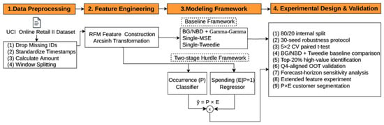
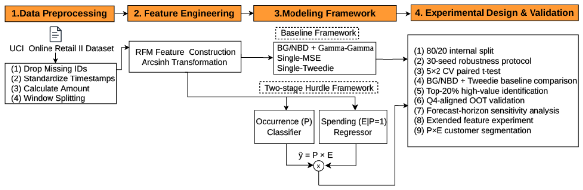
Figure 1 presents the overall research framework of this study. Raw transaction records from the UCI Online Retail II dataset are first preprocessed through removal of records with missing customer IDs, timestamp standardization, amount calculation, and observation/prediction window splitting. RFM features are then constructed from the observation window, while the net-spending target in the prediction window is transformed using the arcsinh function to handle skewness and negative return values. In the proposed two-stage Hurdle framework, the first stage uses an XGBoost classifier to estimate future purchase probability P, whereas the second stage uses gradient-boosting regressors to estimate conditional spending intensity E among buyers. The final CLV prediction is obtained as ŷ = P × E. The framework also incorporates three baseline models for comparison and is evaluated through nine validation dimensions, detailed in Section 5.
Figure 1.
Research framework.
3.1. Data Preprocessing
The Online Retail II dataset from the UCI Machine Learning Repository is used in this study, covering complete transaction records from a UK online retailer between December 2009 and December 2011, totaling 1,067,371 original records. This dataset represents a non-contractual retail setting where customers freely enter and exit at any time [17,18], and has been adopted in multiple comparable studies [7,10], facilitating cross-study comparison.
Data preprocessing includes four operations: removing records with missing customer IDs; standardizing timestamp formats; computing per-transaction amounts (Amount = Quantity × Price); and partitioning by time window. The dataset contains return invoices prefixed with ‘C’ having negative quantities. Return records are explicitly separated from positive transactions, yielding 805,620 positive transactions (97.7%) and 18,744 return records (2.3%). After preprocessing, 824,364 valid records are retained.
The temporal split point is 9 November 2010. The approximately 11-month period before the split (1 December 2009–9 November 2010) serves as the feature period for computing customer behavior indicators. The approximately 44-day period after the split (9 November 2010–23 December 2010) serves as the prediction period and target variable observation window. The prediction period covers Q4 peak season (November–December); this temporal configuration is aligned with the same seasonal cycle in subsequent out-of-time validation (Section 5.6) to ensure fair cross-period comparison.
3.2. Feature Engineering
This study deliberately adopts RFM three-dimensional features as the sole feature source for the main experiment. Some CLV studies enhance prediction accuracy through complex feature architectures, including sequence-to-sequence learning [10] and feature-rich personalized architectures [9]. Such strategies, however, make it difficult to isolate the contribution of model architecture from that of feature engineering. A separate extended feature experiment is included to examine this design decision’s impact (Section 5.7).
RFM features are computed using only positive transaction records, excluding return invoices. RFM captures purchase behavior patterns, while returns are post-purchase behaviors conceptually distinct from purchase decisions. Recency (R) is defined as days between the split date and the customer’s last positive purchase. Frequency (F) is the count of distinct positive invoices in the feature period. Monetary (M) is the total positive transaction amount. This total-monetary definition follows the original RFM framework of Hughes [16], in which M represents the cumulative monetary contribution of a customer rather than the per-transaction average. We acknowledge that total M is moderately correlated with F (r = 0.66, see Section 5.1); however, Section 5.9 shows that F and M occupy complementary rather than redundant roles, with F primarily driving Stage 1 purchase-occurrence predictions and M primarily driving Stage 2 spending–intensity predictions. An average per-transaction monetary definition is a defensible alternative operationalization and is noted as a direction for future comparison.
The target variable is defined as net spending during the prediction period, including return offsets. Unlike the feature construction, the target variable reflects net financial contribution, so negative cash flows from returns are included. Among 4026 customers, 59 (1.47%) have negative net spending (range: −£2945 to approximately £0), 2515 (62.5%) are zero, and 1452 (36.1%) are positive.
The target variable is transformed using the inverse hyperbolic sine function (arcsinh). The traditional log1p transformation (y′ = ln(1 + y)) is undefined when y < −1 and cannot handle the 59 negative values. The arcsinh(y) = ln(y + √(y2 + 1)) is defined over the entire real line, approximating logarithmic behavior for positive values while maintaining symmetry for negative values, and mapping zero to zero, satisfying the co-existence of zero-inflation and negative values.
3.3. Modeling Framework
Mullahy’s [23] Hurdle model decouples the observation-generating mechanism into two independent processes: ‘whether the hurdle is crossed’ and ‘post-crossing intensity.’ In non-contractual retail settings, the applicability of this framework requires further discussion. With only a 44-day prediction window, some zeros may be sampling zeros—customers still active but not transacting within this window—rather than structural zeros. Traditional probabilistic models such as BG/NBD [18] address this distinction through latent attrition mechanisms. In contrast, the Hurdle formulation used here does not explicitly distinguish structural zeros from sampling zeros, which simplifies this distinction.
However, the Hurdle framework’s prediction output ŷ = P(y > 0|X) × E[y|y > 0,X] provides a mathematically interpretable expectation estimate. When the classifier estimates a moderate purchase probability (e.g., P = 0.4) for an active but temporarily non-transacting customer, this probability is multiplied into the conditional amount estimate, producing a non-zero final prediction. The Hurdle architecture therefore does not force all zero-value customers’ predictions to zero. Instead, customers with low but non-zero purchase probability may still receive non-zero final predictions through the multiplicative structure of probability and conditional spending estimates.
Stage 1 (Occurrence Classifier) uses an XGBoost classifier [19] to predict purchase probability P(y > 0|X). Stage 2 (Intensity Regressor) trains a regression model only on the actual buyer subset, predicting conditional spending E[y|y > 0,X]. Stage 2 compares three gradient-boosting algorithms, XGBoost [19], LightGBM [20], and CatBoost [21], with comparable core hyperparameters (n_estimators = 400, learning_rate = 0.05, subsample = 0.8).
Three tiers of baseline models are included for comparison. Tier 1: BG/NBD + Gamma–Gamma [17,18], serving as a well-established probabilistic benchmark. Tier 2: single-stage gradient boosting with MSE loss (Single-MSE), serving as the most direct comparison. Tier 3: single-stage models with Tweedie loss (Single-Tweedie), serving as strong baselines. The Tweedie distribution can represent a point mass at zero and a continuous positive distribution, and has been widely used for zero-inflated claim-type outcomes [15]. XGB–Tweedie and LGB–Tweedie with tweedie_variance_power = 1.5 are included.
3.4. Validation Framework
The validation covers nine dimensions: (1) 80/20 internal split for performance benchmarking; (2) 30-seed robustness protocol controlling training randomness; (3) paired t-test applied to 10 ΔR2 values generated via 5 × 2 cross-validation, following the experimental design of Dietterich [27]; (4) BG/NBD + Tweedie dual-tier baseline comparison; (5) top-20% high-value identification with Precision, Recall, and F1-score; (6) Q4-aligned OOT cross-year validation; (7) forecast-horizon sensitivity analysis; (8) extended feature experiment (RFM + 3); and (9) P × E dual-dimension risk segmentation.
Because the primary objective of this study is to examine the effect of architectural decomposition rather than to identify the universally best algorithm, the main comparisons are conducted within the gradient-boosting family. Holding the boosting engine comparable across single-stage and two-stage settings helps isolate the contribution of the Hurdle architecture from confounding algorithmic differences that would arise from introducing fundamentally different model families (e.g., random forests, support vector machines, or neural networks). BG/NBD + Gamma–Gamma and Tweedie-loss models are further included as probabilistic and distributional baselines, broadening the comparison beyond the gradient-boosting family while keeping the core architectural contrast (single-stage vs. two-stage) uncontaminated by algorithmic confounds.
4. Mathematical Definitions
4.1. RFM Features
Equation (1) defines Recency as the number of days between the split date and the customer’s last positive purchase. A lower R value indicates more recent activity and is associated with higher purchase propensity.
Equation (2) defines Frequency as the count of distinct positive invoices. F reflects transaction frequency and is a key behavioral signal in BG/NBD-type models [18].
Equation (3) defines Monetary as the sum of all positive transaction amounts. In the present RFM implementation, M reflects cumulative spending magnitude over the feature period; this differs from average-transaction-value formulations used in some Gamma–Gamma-type monetary models [26], a distinction discussed further in Section 3.2.
4.2. Target Transformation
Equation (4) is the arcsinh transformation. Unlike log1p (undefined for y ≤ −1), arcsinh maps all reals, handling negative net spending from returns. For y > 0, arcsinh(y) ≈ ln(2y); for y < 0, it remains continuous and monotone, preserving all 59 negative-value customers. In the two-stage framework, arcsinh primarily benefits target representation for single-stage baselines and descriptive statistics; Stage 2 trains exclusively on buyers (y > 0), so the handling of negative values mainly affects the full-sample target distribution rather than the two-stage prediction output directly.
Equation (5) is the binary indicator: customers with positive net spending are labeled 1 (buyers), others 0. This serves as the Stage 1 classifier target.
4.3. Hurdle Prediction
Equation (6) is the Hurdle core. Stage 1 outputs P ∈ [0,1]; Stage 2 outputs conditional spending E. The product P × E provides a mechanism for handling zero-inflated outcomes: when P → 0, ŷ → 0, regardless of E.
4.4. Evaluation Metrics
Equation (7) is the coefficient of determination. R2 = 1 indicates perfect prediction; R2 = 0 equals mean prediction; negative R2 means the model is worse than the mean.
Equation (8) is mean absolute error. MAE weights all errors equally, reflecting typical prediction deviation without extreme-value sensitivity.
Equation (9) is root-mean-squared error. RMSE penalizes large errors quadratically, dominated by high-spending customers in zero-inflated CLV data.
Equation (10) defines Precision (proportion of predicted high-value that are truly high-value) and Recall (proportion of truly high-value that are identified).
Equation (11) is F1-score, the harmonic mean of Precision and Recall. It penalizes imbalance: P = 0.90, R = 0.20 yields F1 = 0.33, not 0.55.
4.5. Directional Consistency Test
Equation (12) is the sign test p-value: n = 10 (5 × 2 CV); k = count of ΔR2 > 0; H0: P(ΔR2 > 0) = 0.5. The t-test checks magnitude; the sign test checks directional consistency. Significant t but non-significant sign test indicates less consistent improvement direction.
5. Results
The sample comprises 4026 customers: 36.07% positive, 62.5% zero, 1.47% negative. The arcsinh-transformed target ranges from −8.68 to 11.93.
5.1. Descriptive Statistics
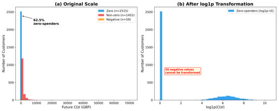
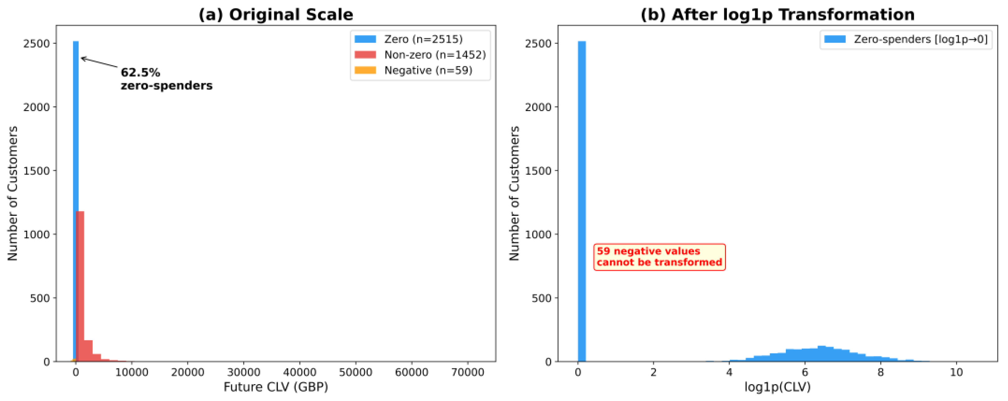
Figure 2 presents the CLV distribution. Panel (a) reveals that 62.5% of customers are zero-spenders with extreme right-skew in the positive tail. Panel (b) shows that log1p transformation cannot handle the 59 customers with negative net spending. These characteristics motivate the adoption of the arcsinh transformation and the two-stage Hurdle architecture.
Figure 2.
CLV distribution: original scale and log1p transformation.
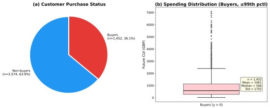
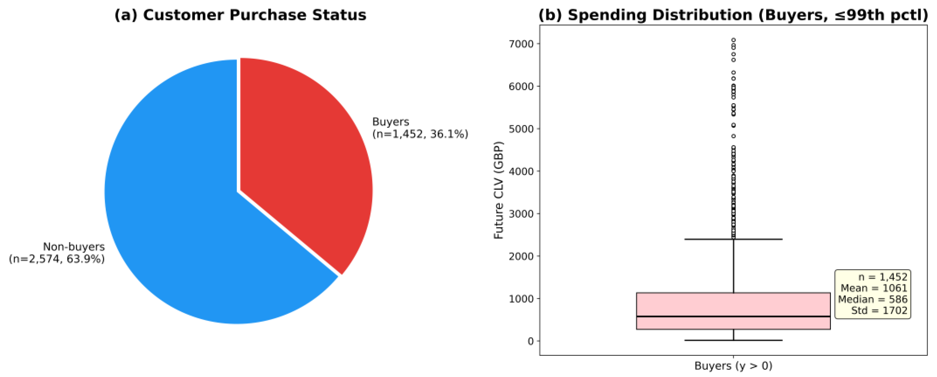
Figure 3 illustrates customer purchase status and spending distribution. Panel (a) shows that 63.9% of customers (n = 2574) are non-buyers and 36.1% (n = 1452) are buyers within the prediction window. Note that the 59 negative-value customers are classified as non-buyers (net spending ≤ 0) despite having transactions, as their product returns exceed purchases within the prediction window. Panel (b) presents the buyer spending distribution truncated at the 99th percentile, with a mean of £1061, a median of £586, and a standard deviation of £1702. The heavy-tailed distribution with substantial outliers supports the use of a separate conditional regression for spending intensity estimation.
Figure 3.
Customer purchase status and spending distribution.
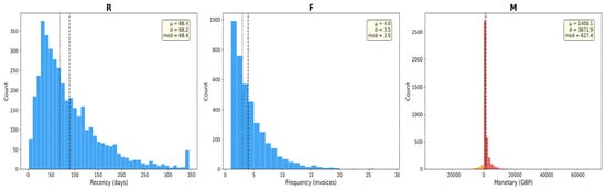
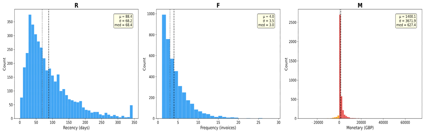
Figure 4 presents the RFM feature distributions. Recency (R) is right-skewed (μ = 88.4 days, med = 68.4 days), indicating that most customers made relatively recent purchases but with a long inactive tail. Frequency (F) is severely right-skewed (μ = 4.0, med = 3.0 invoices), reflecting the dominance of low-frequency buyers. Monetary (M) is strongly right-skewed (μ = £1400, med = £627.4), reflecting the concentration of spending among a small number of high-value customers; as M is computed from positive transaction records only (Section 3.2), it does not itself take negative values. Negative values arise instead in the target variable, where return offsets included in prediction-period net spending produce negative net spending for 59 customers, motivating the adoption of the arcsinh transformation.
Figure 4.
RFM feature distributions.
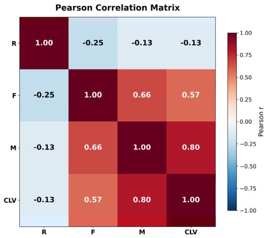
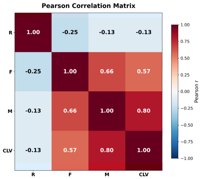
Figure 5 presents the Pearson correlation matrix among RFM features and the CLV target. M–CLV shows the strongest correlation (r = 0.80), followed by F–CLV (r = 0.57), while R–CLV is weakly negative (r = −0.13). The moderate F–M correlation (r = 0.66) indicates partial collinearity between frequency and monetary value. These correlations foreshadow the complementary SHAP feature structures discussed in Section 5.9.
Figure 5.
Pearson correlation matrix.
5.2. Architecture Performance Comparison
Table 1 compares the predictive performance of the three model architectures. The Two-stage CatBoost model achieves the highest R2 value (0.522), outperforming Single-MSE XGBoost (0.385) and XGB–Tweedie (0.309), corresponding to relative R2 improvements of 35.6% and 68.9%, respectively. Across XGBoost, LightGBM, and CatBoost, the two-stage architecture consistently improves R2 compared with its corresponding Single-MSE counterpart. The best-performing two-stage model also shows low seed-to-seed variation (CatBoost SD = 0.008). LGB–Tweedie yields a negative R2 (−0.287), suggesting that the tested Tweedie configuration may be insufficient for this dataset with 62.5% zero-inflation.
Table 1.
Architecture comparison results (arcsinh-transformed target, 30 seeds, mean ± SD).
Table 2 reports the discriminative ability of the Stage 1 XGBoost classifier, evaluated separately using standard binary classification metrics. The classifier achieved an ROC-AUC of 0.739 (±0.002) and an average precision of 0.674 (±0.002) across 30 random seeds, indicating discriminative performance well above chance under the dataset’s 63.9% non-buyer rate (2574 of 4026 customers with zero or negative net spending in the prediction window). The Brier score (0.185 ± 0.001) and calibration slope (0.93 ± 0.01) further indicate that predicted purchase probabilities are reasonably well-calibrated, supporting their use as a continuous risk signal in the P × E segmentation analysis (Section 5.8). A calibration slope of 1.0 indicates perfect calibration; the observed value of 0.93 indicates slight overconfidence—predicted probabilities are marginally more extreme than the observed rates—but remains within an acceptable range for use as a continuous ranking signal.
Table 2.
Stage 1 classifier diagnostic metrics (30 seeds, mean ± SD).
5.3. 5 × 2 CV Paired T-Test and Sign Test
Table 3 reports 5 × 2 CV paired t-test and sign test results. All three algorithms achieve statistically significant t-test results (p < 0.05), indicating that the magnitude of improvement is unlikely to be due to chance. The sign test further examines directional consistency: LightGBM achieves consistency across all 10 comparisons (10/10, p_sign = 0.001), and CatBoost achieves high consistency (9/10, p_sign = 0.011). For XGBoost, the t-test result is significant (p_t = 0.011), but the sign test provides weaker directional evidence (7/10, p_sign = 0.172), suggesting that the improvement direction is less consistent across splits.
Table 3.
The 5 × 2 CV paired t-test and sign test results.
5.4. Baseline Comparison with Tweedie and BG/NBD Models
Table 4 compares the two-stage models with their corresponding single-stage Tweedie-loss baselines. Tweedie models with variance power 1 < p < 2 can accommodate a point mass at zero through the compound Poisson formulation, making them a relevant baseline for zero-inflated positive outcomes. Under the current experimental setting, both two-stage variants significantly outperform their Tweedie counterparts (p < 0.05), with LightGBM showing the largest performance gap. These results suggest that explicitly decoupling purchase occurrence and spending intensity provides higher predictive performance than the tested single-stage Tweedie approach.
Table 4.
Two-stage vs. Tweedie comparison under the 30-seed protocol.
Table 5 ranks all nine models. The performance order is Two-stage CatBoost (R2 = 0.522), Two-stage LightGBM (R2 = 0.465), Two-stage XGBoost (R2 = 0.435), BG/NBD + Gamma–Gamma (R2 = 0.395), and Single-MSE XGBoost (R2 = 0.385). The BG/NBD + Gamma–Gamma model outperforms all Single-MSE models, indicating that probabilistic customer-base modeling remains a strong benchmark for non-contractual CLV prediction. All two-stage models obtain higher R2 values than the BG/NBD + Gamma–Gamma baseline in this experiment, suggesting that the occurrence–intensity architecture provides additional predictive gains under the present zero-inflated retail setting.
Table 5.
Cross-model comparison of all nine models.
5.5. High-Value Customer Identification
Table 6 evaluates top-20% high-value customer identification. All results are computed on the 20% holdout test set. Single-MSE models show high Precision (XGBoost: 0.830) but extremely low Recall (0.185), missing 81.5% of true high-value customers by assigning many of them predicted values below the top-20% threshold. XGB–Tweedie improves Recall to 0.491 (F1 = 0.538). Two-stage models produce more balanced Precision–Recall trade-offs; Two-stage LightGBM achieves the highest F1 among two-stage models (P = 0.618, R = 0.430, F1 = 0.507). It should be noted that XGB–Tweedie achieves the highest overall F1 (0.538) across all models on this identification task. While the two-stage architecture demonstrates superior R2 and RMSE performance, its top-20% F1 does not universally dominate, suggesting that relative strengths depend on the evaluation criterion.
Table 6.
Top-20% high-value customer identification results (threshold = £442.20).
5.6. Temporal Robustness and Forecast-Horizon Sensitivity
Table 7 reports out-of-time validation using the 2011 Q4 prediction window. Two-stage CatBoost maintains the best R2 and RMSE performance (R2 = 0.459, RMSE = 857.05), corresponding to a relative R2 improvement of 17.4% over Single CatBoost (R2 = 0.391). Two-stage CatBoost also shows low seed-to-seed variation in R2 (SD = 0.012). However, Single CatBoost achieves the lowest MAE (221.40), indicating that the two-stage architecture improves explained variance and large-error control but does not uniformly dominate all error metrics. Both periods are aligned to the Q4 holiday season, helping control for seasonal effects across training and validation windows.
Table 7.
OOT cross-year validation results (Q4 2011, 30 seeds).
Table 8 reports a sensitivity analysis conducted beyond the 44-day (Q4 peak period) horizon used in the main experiments, evaluating robustness at 30-, 60-, and 90-day horizons across the three two-stage algorithms. R2 remains positive across all tested horizons but does not increase monotonically for every algorithm, whereas MAE and RMSE generally increase as longer windows accumulate larger absolute spending amounts.
Table 8.
Forecast horizon sensitivity (two-stage models, 30 seeds).
Table 9 isolates the two-stage architecture’s advantage over the Single-MSE CatBoost baseline across forecast horizons. The two-stage model consistently outperforms the baseline, with ΔR2 ranging from +0.086 at 90 days to +0.185 at 30 days. The larger gain under the 30-day horizon is consistent with its higher exact-zero rate (66.6% vs. 56.8% at 90 days), supporting the rationale that occurrence–intensity decomposition is more beneficial under stronger zero-inflation. A shorter prediction window captures fewer repeat purchases, concentrating behavioral differences between buyers and non-buyers into a more pronounced zero-inflation pattern, which amplifies the architectural benefit of separating occurrence from intensity. Here, Exact-Zero % denotes the proportion of customers with exactly zero net spending (y = 0), which differs from the Stage 1 non-buyer rate that also includes negative net spending (y ≤ 0). The 44-day row is included only as a protocol-matched reference and is not intended to reproduce the 30-seed aggregate result in Table 1. Overall, the results indicate that the two-stage advantage is robust across forecast horizons rather than specific to the 44-day Q4 window.
Table 9.
Two-stage advantage by forecast horizon (CatBoost, vs. Single-MSE).
5.7. Extended Feature Experiment
Table 10 adds three extended features (average order value, return rate, purchase interval CV) to the RFM feature set. Two-stage XGBoost improves marginally from 0.435 to 0.440 (ΔR2 = +0.005)—substantially smaller than the R2 gains observed under the main RFM experiment. In contrast, Two-stage CatBoost declines from 0.522 to 0.427 under the extended feature set, suggesting that these additional features may introduce noise that disrupts CatBoost’s optimization under present dataset conditions. This suggests that the observed performance gains are more likely attributable to the two-stage architecture than to the addition of these extended features, though the CatBoost result also indicates that architectural advantage may not be uniformly robust under feature set changes.
Table 10.
Extended feature experiment results (RFM + 3, 30 seeds).
This degradation is consistent with a structural property of CatBoost: its symmetric (oblivious) tree growth applies the same split rule across all nodes at a given depth, which is efficient for low-dimensional homogeneous feature spaces but becomes constrained when weakly correlated features are added. XGBoost and LightGBM grow asymmetric trees and can route branches around uninformative features more flexibly, explaining the absence of a comparable decline for those algorithms.
5.8. P × E Customer Segmentation
Table 11 segments customers by purchase probability (P) and conditional spending intensity (E). All results are computed on the 20% holdout test set (n = 806). The Dormant, High-E segment (n = 96) has an actual purchase rate of only 26% despite high conditional spending (E = £637). Ranking solely by CLV = P × E may therefore lead to inefficient resource allocation by prioritizing customers with high expected spending but relatively low purchase probability. Applying a P ≥ 0.3 screening threshold before E-based ranking improves effective coverage from 26% to 64%. The P × E formulation is an intentional design choice: it preserves purchase uncertainty as a continuous quantity rather than collapsing P into a binary buy/no-buy decision before computing expected spending. Restricting the revenue calculation to customers predicted to purchase above some probability threshold would discard the graded information contained in P and would require an arbitrary threshold choice upstream of the spending estimate. The P ≥ 0.3 screening procedure reported above can be viewed as a practical hybrid of the two approaches: P is used as a coarse filter, while E retains its role as the within-segment ranking criterion, combining the interpretability of a threshold-based rule with the continuous information content of the P × E expectation.
Table 11.
P × E dual-dimension customer segmentation results.
5.9. SHAP Model Interpretability Analysis
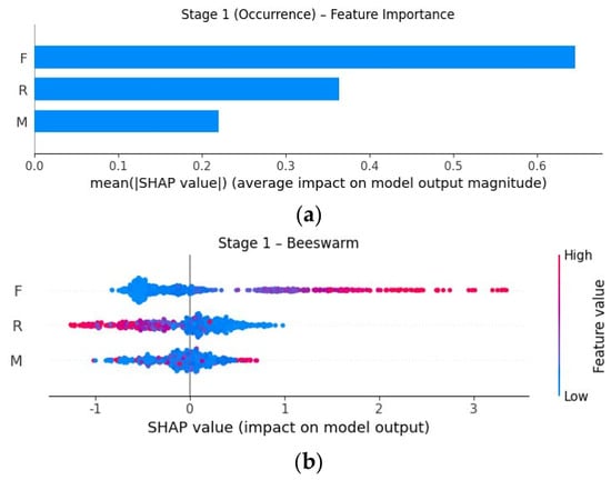
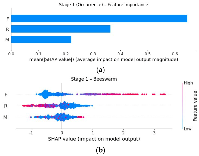
Figure 6 presents Stage 1 SHAP importance. Consistent with recent applications of SHAP in customer analysis [28,29], feature contributions are decomposed at both global and individual levels. The bar plot shows that F has the highest mean absolute SHAP value (0.645), substantially exceeding R (0.363) and M (0.220). The beeswarm plot further reveals that high F values are associated with positive SHAP contributions to the predicted purchase probability, whereas high R values are associated with negative contributions. This frequency-dominant ranking is consistent with customer-base models such as BG/NBD, in which transaction frequency is a key signal of future purchase activity [17].
Figure 6.
Stage 1 SHAP feature importance: (a) mean absolute SHAP values (F > R > M); (b) beeswarm plot of directional contributions.
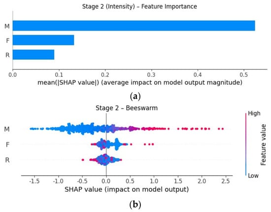
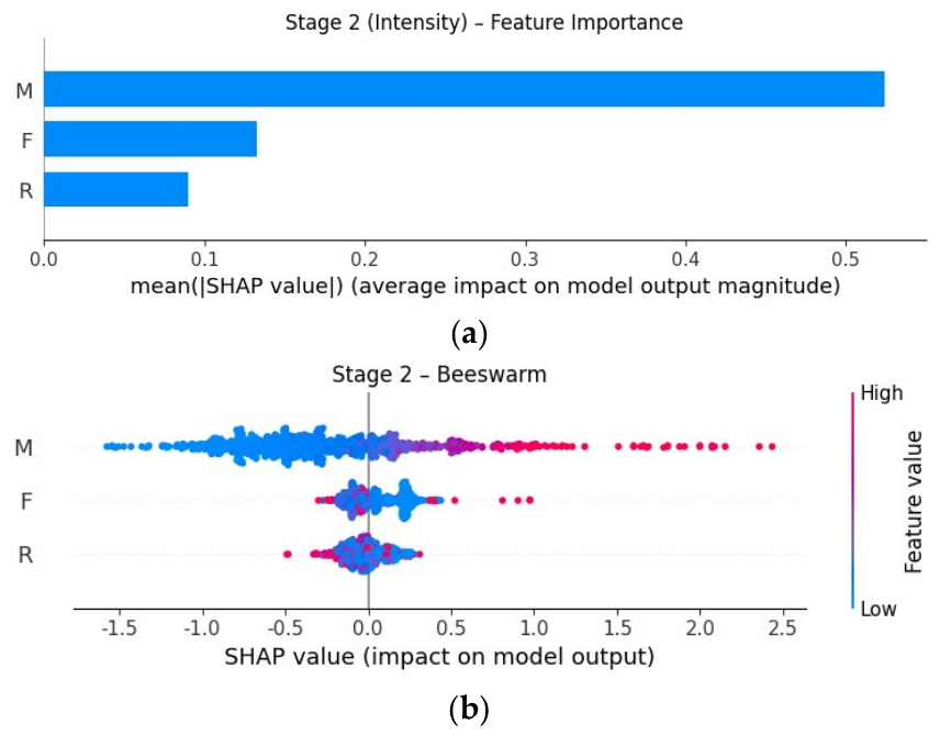
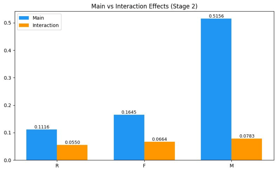
Figure 7 presents Stage 2 SHAP importance. The feature ranking is reversed compared with Stage 1, with M achieving the highest mean absolute SHAP value (0.524), followed by F (0.133) and R (0.090). Note that the mean |SHAP| value (0.524) and the main effect decomposition reported in Figure 8 (0.5156) represent different analytical perspectives—the former aggregates absolute contributions while the latter decomposes into main and interaction components—and are therefore not directly comparable. The beeswarm plot confirms that high M values are associated with positive SHAP contributions to conditional spending intensity. This monetary-dominant pattern is consistent with the Gamma–Gamma model, which uses historical monetary value to model conditional transaction value [26]. The complementary feature structure across Stage 1 (F-dominant) and Stage 2 (M-dominant) supports the rationale of the Hurdle architecture in separating purchase occurrence from spending intensity.
Figure 7.
Stage 2 SHAP feature importance: (a) mean absolute SHAP values (M > F > R); (b) beeswarm plot of directional contributions.
Figure 8.
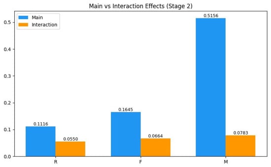
Main vs. interaction effects (Stage 2).
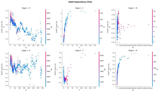
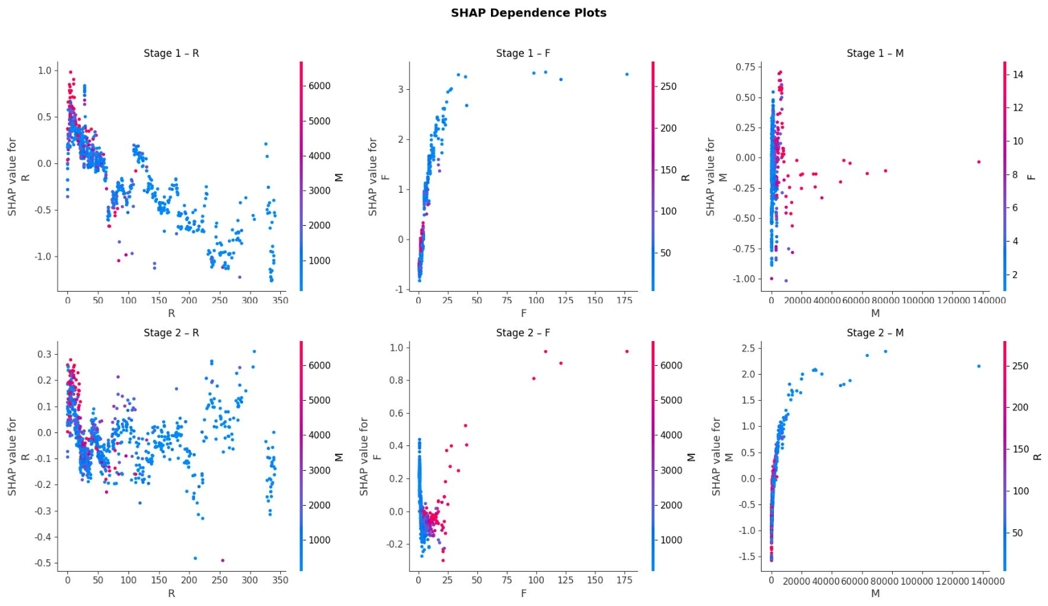
Figure 9 presents SHAP dependence plots for all three RFM features across Stage 1 and Stage 2. Two key patterns are highlighted. In Stage 1, Frequency exhibits a step-like effect: SHAP values rise sharply from F = 0 to approximately F = 3 and then gradually saturate, indicating that purchase probability is most sensitive to frequency changes among low-frequency customers. In Stage 2, Monetary shows an approximately positive relationship with conditional spending intensity, with increasing variance at high M values, reflecting greater prediction uncertainty for high-spending customers.
Figure 9.
SHAP dependence plots (top: Stage 1; bottom: Stage 2).
Figure 8 decomposes Stage 2 SHAP values into main effects and interaction effects. M’s main effect accounts for 87% of its total SHAP contribution, indicating that Monetary’s contribution is dominated by its main effect rather than interactions with other features. Frequency shows a higher interaction proportion (29%), suggesting that F’s effect on spending intensity is more conditional on other features.
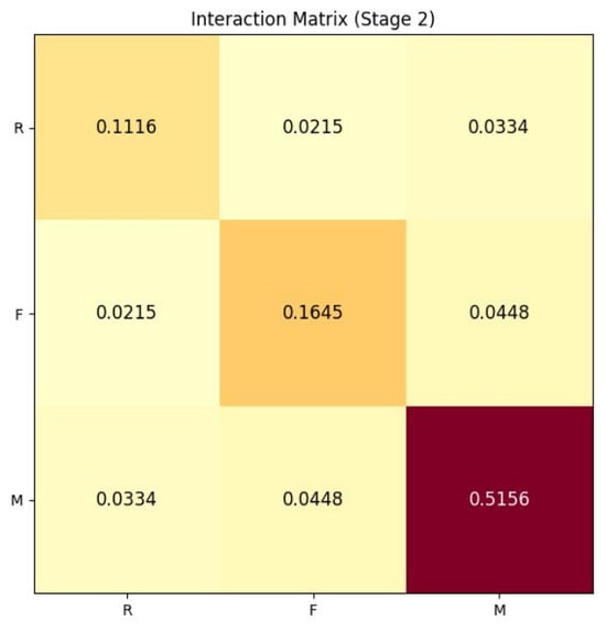
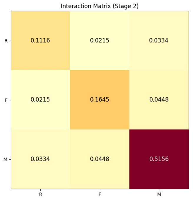
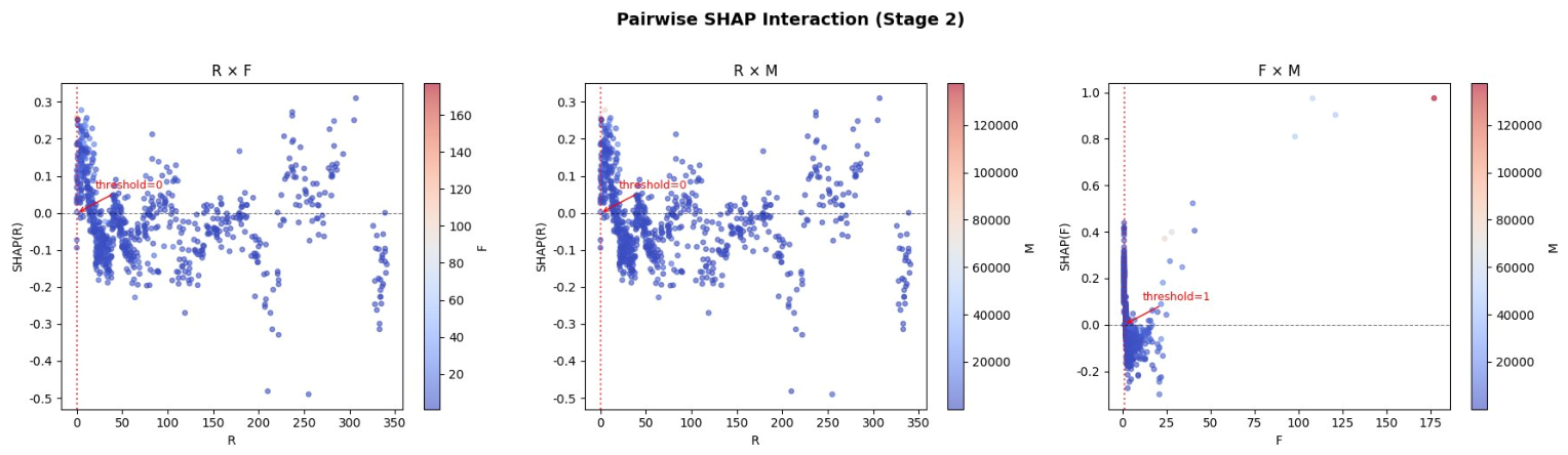
Figure 10 presents the Stage 2 SHAP interaction matrix. The strongest pairwise interaction is F × M (0.0448), suggesting that frequency and monetary value jointly contribute to conditional spending prediction in addition to their individual main effects. M × R (0.0334) is secondary, and F × R (0.0215) is the weakest pair.
Figure 10.
Stage 2 SHAP interaction matrix (F × M = 0.0448 is the strongest pair). Color intensity indicates interaction strength; darker colors represent stronger pairwise interactions.
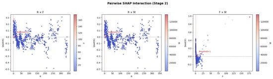
Figure 11 visualizes pairwise SHAP interactions for Stage 2. The F × M panel shows relatively stronger positive interactions among customers with higher monetary value, particularly when frequency is not extremely high, suggesting a joint contribution of monetary value and frequency to conditional spending predictions. The M × R panel shows weaker and more dispersed interactions. The F × R panel also shows relatively weak interactions, with no comparably concentrated positive pattern. Overall, the pairwise plots are consistent with the interaction matrix in Figure 10, where F × M is the strongest pairwise interaction.
Figure 11.
Pairwise SHAP interaction scatter plots for F × M, M × R, and F × R pairs.
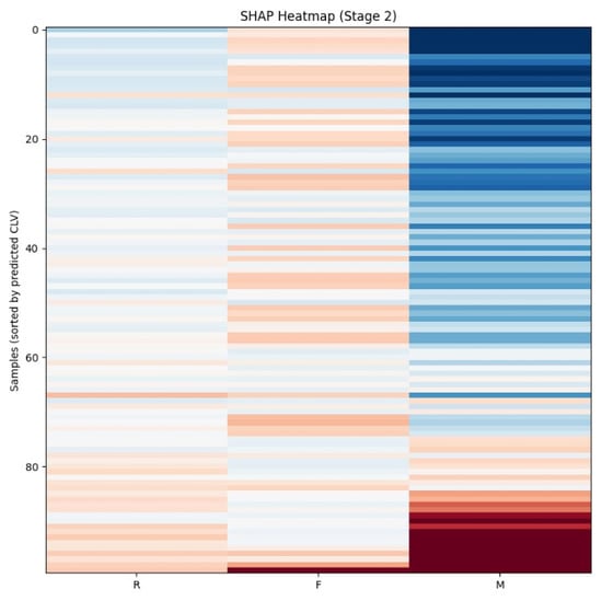
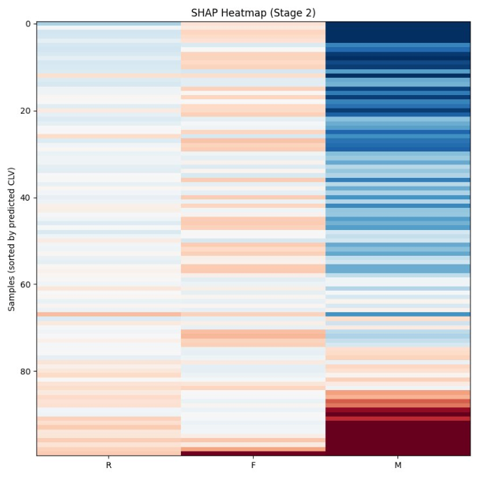
Figure 12 presents a SHAP heatmap of 100 customers sorted by predicted CLV. In the high predicted-CLV region, M shows strong positive SHAP contributions, often accompanied by positive F contributions. In the lower predicted-CLV region, M transitions toward negative contributions (blue), while lower-frequency customers tend to show more negative F contributions, especially in this region. The heatmap illustrates that high M together with positive F contributions characterizes customers with elevated predicted CLV.
Figure 12.
SHAP heatmap (100 samples, sorted from low to high predicted CLV). Red indicates positive SHAP contributions; blue indicates negative SHAP contributions.
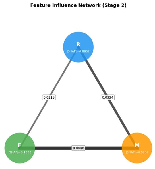
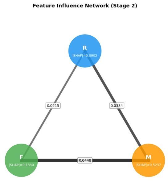
Figure 13 visualizes Stage 2 feature interactions as a network. Node size reflects main effect magnitude, and edge thickness reflects pairwise interaction strength. M is the largest node (mean |SHAP| = 0.5237; main effect = 0.5156), and the F–M edge is the thickest (0.0448), consistent with the interaction matrix in Figure 10. M and F are the two most influential features in the network, whereas R shows comparatively smaller main effect and interaction contributions.
Figure 13.
Feature influence network (Stage 2).
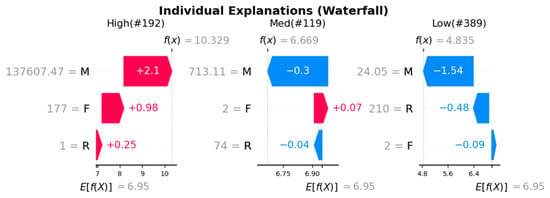
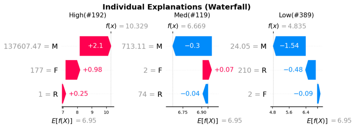
Figure 14 shows waterfall plots for three representative customers. High (#192, f(x) = 10.329): M = £137,607 contributes the largest positive SHAP (+2.1), F = 177 adds secondary support (+0.98), and R = 1 provides additional positive contribution (+0.25). Med (#119, f(x) = 6.669): near the baseline with moderate M = £713 (−0.3) and low F = 2 (+0.07). Low (#389, f(x) = 4.835): M = £24 generates the strongest negative SHAP (−1.5), with high R = 210 contributing an additional negative effect (−0.48). The waterfall plots support individual-level interpretation of prediction behavior.
Figure 14.
Individual SHAP waterfall explanations.
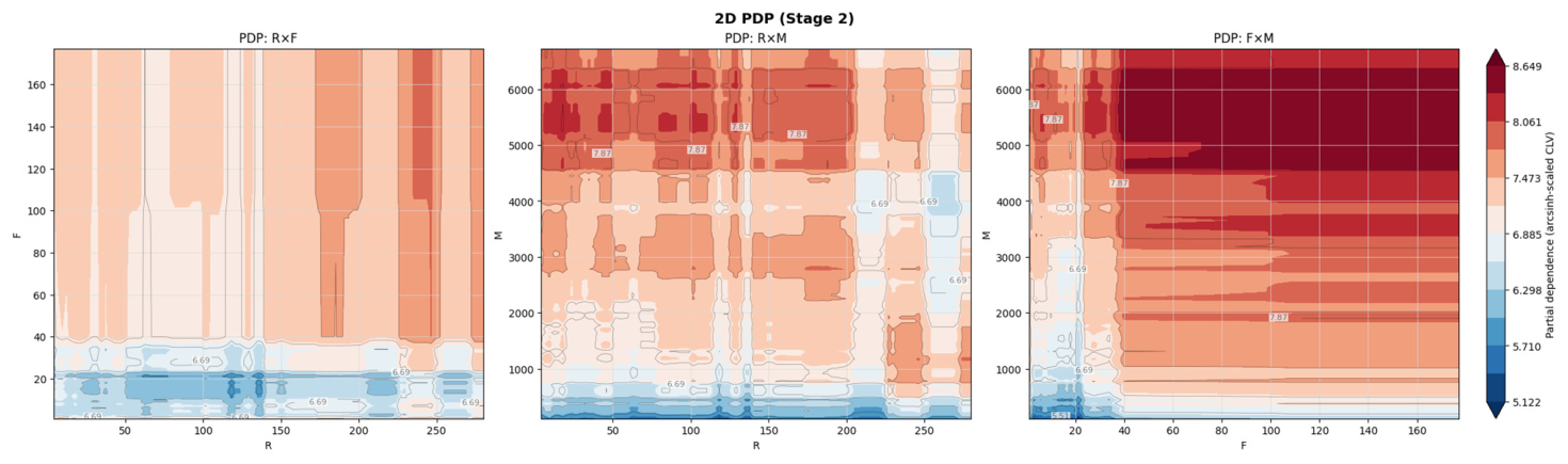
Figure 15 presents 2D Partial Dependence Plots for Stage 2. The R × F surface shows the highest predicted conditional spending intensity at low R and high F, consistent with recently active and high-frequency customers receiving the strongest predictions. The R × M surface shows that high M combined with low R is associated with higher predicted conditional spending, indicating that recent high-spending customers are most strongly predicted. The F × M surface shows a nonlinear increase in predicted conditional spending at high F and high M, suggesting nonlinear joint effects between frequency and monetary value.
Figure 15.
2D Partial Dependence Plots (Stage 2).
6. Discussion
6.1. Evidence for Architectural Effectiveness
The consistent R2 improvements observed across XGBoost, LightGBM, and CatBoost suggest that the performance gains are more likely attributable to the architectural principle of occurrence–intensity decoupling rather than to algorithm-specific tuning or parameter optimization. In zero-inflated data, purchase occurrence and conditional spending magnitude arise from structurally distinct behavioral processes: a customer’s decision to purchase at all is not governed by the same mechanism as the amount spent once a purchase is made. Forcing a single regression model to handle both simultaneously creates a distributional mismatch that the two-stage architecture is specifically designed to avoid.
This interpretation is further supported by the statistical validation results. The paired t-test applied to 10 ΔR2 values from 5 × 2 cross-validation indicates that the improvements hold across repeated random reshufflings, and the sign test reveals that for LightGBM and CatBoost, the two-stage architecture outperforms its single-stage counterpart in the majority of individual splits. These findings imply that the architectural advantage is not an artifact of a favorable data partition. It is worth noting that the 5 × 2 CV ΔR2 values (Table 3) differ from the within-algorithm gains implied by Table 1: for instance, CatBoost shows a large 80/20 improvement (+0.174) but a smaller 5 × 2 CV mean ΔR2 (+0.072). This difference is expected, as each 5 × 2 CV fold uses only 50% of available training data, which compresses architectural gains—particularly for CatBoost, which benefits more from larger training sets. LightGBM consistently shows the strongest 5 × 2 CV evidence (ΔR2 = 0.177, 10/10, p_sign = 0.001), making it the most statistically robust demonstration of architectural benefit, even though Two-stage CatBoost achieves the highest absolute R2 under the 80/20 protocol.
From a methodological standpoint, this result carries a practical implication: in non-contractual retail settings with high proportions of non-purchasing customers, the primary modeling decision may lie in architectural design rather than in the selection of more complex algorithms or elaborate feature engineering. Future CLV research operating under similar distributional conditions may benefit from treating occurrence and intensity as separate modeling targets.
6.2. Comparison of Zero-Inflation Handling Mechanisms
Three zero-inflation handling strategies were compared, with performance ranking: Two-stage Hurdle > Single-MSE > Tweedie. The relatively weak performance of the Tweedie baselines deserves further discussion. XGB–Tweedie (R2 = 0.309) falls below Single-MSE XGBoost (0.385), and LGB–Tweedie produces negative R2. This may stem from insufficient tuning of the variance power parameter (variance_power = 1.5), or the tested Tweedie specification may not fully capture the distributional characteristics of this dataset. A systematic sensitivity sweep over variance_power ∈ [1.1, 1.99] is reported below (Table 12) to determine whether an optimized Tweedie configuration can narrow the performance gap.
Table 12.
Tweedie variance power sensitivity analysis.
Table 12 reports a sensitivity analysis conducted across tweedie_variance_power ∈ [1.1, 1.99] to assess whether the Tweedie baseline’s underperformance stems from suboptimal hyperparameter selection rather than an architectural limitation. Because this sensitivity sweep was conducted under a dedicated single-protocol setting designed to characterize the shape of the R2–variance-power relationship, its p = 1.5 result differs slightly from the 30-seed aggregate Tweedie baseline reported in Table 1. XGB–Tweedie’s R2 improved monotonically from 0.170 (p = 1.1) to a maximum of 0.470 (p = 1.97), while LGB–Tweedie improved from −0.230 to 0.391 over the same range. Even at the optimized variance power, both Tweedie variants remain below the Two-stage CatBoost model (R2 = 0.522), though the performance gap narrows substantially relative to the default setting (p = 1.5: ΔR2 = 0.229; p = 1.97: ΔR2 = 0.052). This indicates that the two-stage architecture’s advantage over the Tweedie approach is robust to variance power selection rather than an artifact of an unfavorably configured baseline.
6.3. SHAP Analysis and Theoretical Alignment
The SHAP feature structure provides a pattern that is consistent with the theoretical emphasis of established customer-base models. Stage 1’s dominance by F (mean |SHAP| = 0.645) is consistent with BG/NBD, in which transaction frequency is a key signal of future purchase activity [17]. Stage 2’s dominance by M (0.524) is consistent with the Gamma–Gamma model, in which historical monetary value is used to model conditional transaction value [26]. That a gradient-boosting framework trained purely on prediction loss produces feature patterns consistent with these theoretical expectations lends support to the interpretability of the model outputs. The F × M interaction (0.0448) further suggests a joint contribution of Frequency and Monetary value to conditional spending predictions. This complementary structure is an empirical finding rather than a definitional artifact: all three RFM features (R, F, M) are supplied to both Stage 1 and Stage 2 without pre-assignment, and the gradient-boosting models are free to assign importance to any feature at either stage. The observed concentration of importance, F at Stage 1 and M at Stage 2, therefore reflects a pattern learned from data rather than a structural constraint of the modeling pipeline. Its convergence with independently developed customer-base theory (BG/NBD, Gamma–Gamma) is presented as an empirical consistency check rather than a theoretical claim, and is offered as a secondary observation consistent with established theory.
6.4. P × E Risk and Practical Recommendations
The P × E segmentation analysis reveals potential commercial risk in the Hurdle prediction output. The 96 Dormant, High-E customers have an actual purchase rate of only 26%, yet their predicted CLV may remain elevated because of high conditional spending estimates. In practical deployment, a two-stage screening strategy is recommended: apply a P threshold (e.g., P ≥ 0.3) to exclude low-purchase-probability groups, then rank by E to allocate resources. This comparison suggests that probability screening may reduce inefficient allocation, improving effective coverage from 26% to 64%.
6.5. Limitations
The present study has several limitations. Data scope is limited to a single UK retailer; cross-industry and cross-market generalizability requires further validation. The extended feature experiment adds only three derived variables; whether architectural advantage persists in higher-dimensional feature spaces remains an open question. While the Tweedie baseline’s variance_power was examined through a dedicated sensitivity sweep (Table 12), other Tweedie hyperparameters (e.g., learning rate, tree depth) and their potential interaction with variance_power were not jointly optimized, so the reported Tweedie performance may still not represent its full achievable potential. Stage 1 is fixed as XGBoost; optimal classifier selection and Stage 1–Stage 2 pairing strategies warrant systematic evaluation. This study adopts a revenue-based CLV proxy rather than a strict discounted-profit formulation, as cost, margin, and customer-lifetime (attrition) data are unavailable in the UCI Online Retail II dataset. The reported outcome is therefore more precisely characterized as expected net spending within a fixed prediction window rather than CLV in its full discounted-profit sense. Future work incorporating cost structures and survival-based lifetime estimation would enable a more complete CLV operationalization. The Heckman selection model represents a theoretically related two-stage econometric benchmark; it was not included because its identification strategy requires a valid exclusion restriction (a variable affecting purchase occurrence but not conditional spending) that cannot be credibly specified within the present RFM-based feature set, and because its estimation objective (consistent parameter inference under a bivariate-normality assumption) differs from the predictive-accuracy objective evaluated in this study. A methodologically careful comparison against the Heckman model is left for future work.
7. Conclusions
This study applied a two-stage Hurdle gradient-boosting framework to zero-inflated non-contractual CLV prediction using the UCI Online Retail II dataset (4026 customers, 62.5% zero-inflation rate).
The Two-stage CatBoost model achieves R2 = 0.522, corresponding to relative R2 improvements of 35.6% over Single-MSE XGBoost (0.385), 68.9% over XGB–Tweedie (0.309), and surpassing BG/NBD + Gamma–Gamma (0.395). All three gradient-boosting algorithms show consistent R2 improvement under the two-stage architecture, suggesting that the gains are attributable to architectural design rather than algorithm-specific characteristics. The 5 × 2 CV paired t-test indicates statistically significant improvements across all algorithms (p < 0.05), and the sign test indicates strong directional consistency for LightGBM (10/10) and CatBoost (9/10).
SHAP analysis reveals a complementary feature structure: Frequency is the dominant feature in Stage 1 (0.645), consistent with customer-base models such as BG/NBD, while Monetary dominates Stage 2 (0.524), consistent with the Gamma–Gamma model. The P × E dual-dimension segmentation identifies 96 Dormant, High-E customers with an only-26% actual purchase rate. Applying a P ≥ 0.3 screening threshold before E-based ranking improves effective coverage from 26% to 64%, suggesting a potential reduction in inefficient allocation to low-probability customers.
Future work may explore: full joint optimization of Tweedie-related hyperparameters (e.g., learning rate and tree depth, in interaction with variance power); validation across other industries and markets; architectural advantage under high-dimensional feature spaces; and evaluation of alternative Stage 1 classifiers and Stage 1–Stage 2 pairing strategies.
Author Contributions
Conceptualization, C.-Y.L. and Y.-M.C.; methodology, C.-Y.L.; software, C.-Y.L.; validation, C.-Y.L., C.-C.K., C.-E.Y. and Y.-Y.L.; formal analysis, C.-Y.L. and Y.-Y.L.; investigation, C.-Y.L., C.-C.K. and C.-E.Y.; data curation, C.-Y.L.; writing—original draft preparation, C.-Y.L.; writing—review and editing, Y.-M.C., C.-C.K., C.-E.Y. and Y.-Y.L.; visualization, C.-Y.L.; supervision, Y.-M.C.; project administration, Y.-M.C. All authors have read and agreed to the published version of the manuscript.
Funding
This research was funded by the National Science and Technology Council (NSTC), Taiwan, ROC, under Grant No. NSTC-112-2410-H-006-085.
Institutional Review Board Statement
Not applicable. This study used a publicly available secondary dataset (UCI Online Retail II) and did not involve human subjects.
Informed Consent Statement
Not applicable.
Data Availability Statement
The UCI Online Retail II dataset used in this study is publicly available at the UCI Machine Learning Repository: https://archive.ics.uci.edu/dataset/502/online+retail+ii (accessed on 27 May 2026).
Acknowledgments
This research was supported by the National Science and Technology Council (NSTC), Taiwan, ROC, under Grant No. NSTC-112-2410-H-006-085.
Conflicts of Interest
The authors declare no conflicts of interest.
References
- Verhoef, P.C.; Broekhuizen, T.; Bart, Y.; Bhattacharya, A.; Dong, J.Q.; Fabian, N.; Haenlein, M. Digital transformation: A multidisciplinary reflection and research agenda. J. Bus. Res. 2021, 122, 889–901. [Google Scholar] [CrossRef] [Scilit]
- Yan, Y.; Resnick, N. A high-performance turnkey system for customer lifetime value prediction in retail brands. Quant. Mark. Econ. 2024, 22, 169–192. [Google Scholar]
- Kumar, V.; Reinartz, W. Customer Relationship Management, 4th ed.; Springer: New York, NY, USA, 2024. [Google Scholar]
- Reinartz, W.J. Customer relationship management: Past, present, and future. Int. J. Res. Mark. 2026, 43, 8–27. [Google Scholar]
- Duan, N. Smearing estimate: A nonparametric retransformation method. J. Am. Stat. Assoc. 1983, 78, 605–610. [Google Scholar] [CrossRef] [Scilit]
- Manning, W.G. The logged dependent variable, heteroscedasticity, and the retransformation problem. J. Health Econ. 1998, 17, 283–295. [Google Scholar] [CrossRef] [Scilit] [PubMed]
- Sun, Y.; Liu, H.; Gao, Y. Research on CLV based on machine learning. Heliyon 2023, 9, e13384. [Google Scholar] [PubMed]
- Khan, Z.; Ali, A.; Aldahmani, S.; Nordmark, H.; Lausen, B. Customer lifetime value modeling via two stage selected trees ensembles. IEEE Access 2025, 13, 115236–115247. [Google Scholar] [CrossRef] [Scilit]
- Zhao, S.; Wu, R.; Tao, J.; Qu, M.; Zhao, M.; Fan, C.; Zhao, H. perCLTV: A general system for personalized customer lifetime value prediction in online games. ACM Trans. Inf. Syst. 2023, 41, 1–29. [Google Scholar] [CrossRef] [Scilit]
- Bauer, J.; Jannach, D. Improved CLV prediction with sequence-to-sequence learning. ACM Trans. Knowl. Discov. Data 2021, 15, 1–37. [Google Scholar]
- Boucher, J.-P.; Denuit, M.; Guillén, M. Risk classification for claim counts: A comparative analysis of various zero-inflated mixed Poisson and hurdle models. N. Am. Actuar. J. 2007, 11, 110–131. [Google Scholar]
- Feng, C.X. A comparison of zero-inflated and hurdle models for modeling zero-inflated count data. J. Stat. Distrib. Appl. 2021, 8, 8. [Google Scholar] [PubMed]
- Xu, X.; Ye, T.; Gao, J.; Chu, D. Generalized hurdle count data models based on interpretable machine learning with an application to health care demand. Computing 2024, 106, 295–325. [Google Scholar]
- Senocak, A.U.G.; Yilmaz, M.T.; Kalkan, S.; Yucel, I.; Amjad, M. An explainable two-stage ML approach for precipitation forecast. J. Hydrol. 2023, 627, 130375. [Google Scholar]
- So, B. Enhanced gradient boosting for zero-inflated insurance claims and comparative analysis of CatBoost, XGBoost, and LightGBM. Scand. Actuar. J. 2024, 2024, 1013–1035. [Google Scholar]
- Hughes, A.M. Strategic Database Marketing; Probus: Chicago, IL, USA, 1994. [Google Scholar]
- Schmittlein, D.C.; Morrison, D.G.; Colombo, R. Counting your customers. Manag. Sci. 1987, 33, 1–24. [Google Scholar] [CrossRef] [Scilit]
- Fader, P.S.; Hardie, B.G.S.; Lee, K.L. Counting your customers the easy way. Mark. Sci. 2005, 24, 275–284. [Google Scholar] [CrossRef] [Scilit]
- Chen, T.; Guestrin, C. XGBoost: A scalable tree boosting system. In Proceedings of the 22nd ACM SIGKDD International Conference on Knowledge Discovery and Data Mining, San Francisco, CA, USA, 13–17 August 2016; pp. 785–794. [Google Scholar]
- Ke, G.; Meng, Q.; Finley, T.; Wang, T.; Chen, W.; Ma, W.; Ye, Q.; Liu, T.Y. LightGBM: A highly efficient gradient boosting decision tree. In Proceedings of the 31st International Conference on Neural Information Processing Systems, Long Beach, CA, USA, 4–9 December 2017; pp. 3146–3154. [Google Scholar]
- Prokhorenkova, L.; Gusev, G.; Vorobev, A.; Dorogush, A.V.; Gulin, A. CatBoost: Unbiased boosting with categorical features. In Proceedings of the 32nd International Conference on Neural Information Processing Systems, Montreal, QC, Canada, 2–8 December 2018; pp. 6638–6648. [Google Scholar]
- Curiskis, S.; Dong, X.; Jiang, F.; Scarr, M. A novel approach to predicting CLV in B2B SaaS companies. J. Mark. Anal. 2023, 11, 587–601. [Google Scholar]
- Mullahy, J. Specification and testing of some modified count data models. J. Econom. 1986, 33, 341–365. [Google Scholar] [CrossRef] [Scilit]
- Reinartz, W.J.; Kumar, V. The impact of customer relationship characteristics. J. Mark. 2003, 67, 77–99. [Google Scholar] [CrossRef] [Scilit]
- Mosaddegh, A.; Albadvi, A.; Sepehri, M.M.; Teimourpour, B. Dynamics of customer segments: A predictor of customer lifetime value. Expert Syst. Appl. 2021, 172, 114606. [Google Scholar] [CrossRef] [Scilit]
- Fader, P.S.; Hardie, B.G.S.; Lee, K.L. RFM and CLV: Using iso-value curves for customer base analysis. J. Mark. Res. 2005, 42, 415–430. [Google Scholar] [CrossRef] [Scilit]
- Dietterich, T.G. Approximate statistical tests for comparing supervised classification learning algorithms. Neural Comput. 1998, 10, 1895–1923. [Google Scholar] [CrossRef] [Scilit] [PubMed]
- Yılmaz Benk, G.; Badur, B.; Mardikyan, S. A new 360° framework to predict customer lifetime value for multi-category e-commerce companies using a multi-output deep neural network and explainable artificial intelligence. Information 2022, 13, 373. [Google Scholar]
- Peng, K.; Peng, Y.; Li, W. Research on customer churn prediction and model interpretability analysis. PLoS ONE 2023, 18, e0289724. [Google Scholar] [CrossRef] [Scilit] [PubMed]

Disclaimer/Publisher’s Note: The statements, opinions and data contained in all publications are solely those of the individual author(s) and contributor(s) and not of MDPI and/or the editor(s). MDPI and/or the editor(s) disclaim responsibility for any injury to people or property resulting from any ideas, methods, instructions or products referred to in the content. |
© 2026 by the authors. Licensee MDPI, Basel, Switzerland. This article is an open access article distributed under the terms and conditions of the Creative Commons Attribution (CC BY) license.