


Abstract
Many continuous industrial processes are non-linear, multi-variable, subject to transport or reaction delays, and described by operating-point-dependent parameters. These characteristics reduce the reliability of fixed models used in model predictive control (MPC), particularly when slow disturbances, regime changes and operational constraints are dominant. This paper proposes an output-bias reference-correction framework based on Long Short-Term Memory (LSTM) networks for predictive control of industrial processes with delays and variable parameters. The dominant dynamics are represented by a fixed compact linear nominal model in deviation coordinates; this model drives a standard constrained MPC that remains structurally unchanged throughout operation. The persistent output bias between the actual process and the nominal model is learned from closed-loop data by an LSTM network. At each sampling step, the predicted bias is used to correct the future reference trajectory fed to the nominal MPC, so that the controller compensates for model–process mismatch without modifying its internal model, constraint set or solver. The final implementation uses a one-step bias predictor, selected by ablation, and it extends this one-step estimate across the MPC horizon by exponentially decayed persistence. A closed-loop bias-error bound links the LSTM identification error, the adaptive correction gain and the resulting tracking deviation. The framework is illustrated using a mining thickener, a representative process characterised by slow dynamics, delays, variable parameters and stringent safety constraints. A three-controller Monte Carlo study compares the nominal MPC, a classical offset-free MPC and the proposed LSTM-MPC, and it highlights the resulting tracking–actuation–constraint trade-off. Applied to a mining thickener, the LSTM corrector reduces the first-step output-prediction RMSE by 96.6% (FIT from to ). In a 50-scenario Monte Carlo closed-loop evaluation, the LSTM-MPC outperforms the nominal MPC in 92% of scenarios on RMSE while using substantially less actuator activity than the offset-free baseline (mean input total variation: 67.0 vs. 119.4).
1. Introduction
Continuous industrial processes encountered in the chemical, hydrometallurgical, environmental and mining sectors frequently involve a combination of phenomena that make them difficult to control. They are often multivariable, highly coupled, constrained by safety limits, and affected by delays associated with material transport, mixing times, slow reactions, sensors or actuators. Furthermore, the dynamic parameters of the process vary with the operating point, the quality of the feedstock, fouling, temperature, equipment ageing or hydraulic load. These processes can therefore be described as systems with delays and variable parameters.
In this context, model predictive control (MPC) is a particularly suitable approach. It enables the future behaviour of the process to be anticipated, explicitly accounts for constraints on inputs and outputs, and manages multivariable interactions [1,2,3,4]. Nevertheless, the performance of MPC depends heavily on the quality of the prediction model. A single linear invariant model may prove inadequate when the process changes regime, when effective time delays vary, or when unmeasured phenomena alter the actual dynamics [5,6].
LPV models, Linear Parameter-Varying, offer a compromise between interpretability and flexibility. They adapt the model matrices to a vector of measured or estimated parameters, known as the scheduling vector, and thus enable the local evolution of the dynamics to be represented at the operating point [7,8,9]. LPV models with delays are therefore attractive for slow industrial processes, as they retain a structure that can be exploited by the control system whilst describing transport effects and regime changes. However, their identification becomes challenging when the dominant phenomena include long-term memory effects, local non-linearities, unmeasured disturbances or calibration errors [10].
In contrast, machine learning models, and in particular recurrent neural networks such as LSTM, can capture long-term temporal dependencies and complex non-linearities [11,12,13]. The integration of learning methods within MPC has attracted growing interest, as surveyed in [14]. However, integrating a neural network directly as a complete process model within an MPC loop remains challenging in an industrial environment. The main limitations are the loss of interpretability, the difficulty of extrapolating beyond the training domain, the computational cost of multi-horizon predictions, and the complexity of ensuring compliance with constraints [14,15].
This article takes the middle ground. The nominal physical or semi-empirical model is not replaced by a neural network. It remains responsible for the dominant dynamics, time delays, and constraint management. The nominal MPC runs structurally unchanged: the same model, the same solver, the same horizons and constraints as a standard implementation. The recurrent network does not modify the internal model of the MPC; instead, it learns the persistent output bias—the difference between the actual process output and the nominal model prediction—and forecasts this bias over the MPC prediction horizon. The forecast is then used to shift the reference trajectory fed to the MPC, so that the controller proactively compensates for the anticipated model–process mismatch. This output-bias reference-correction strategy, inspired by the offset-free MPC literature [16] and the residual learning paradigm [17,18], keeps the MPC layer fully standard while adding adaptivity through the reference channel only.
The proposed framework is general in nature: it applies to industrial processes involving time delays and variable parameters, for which an approximate nominal model and historical data are available. The mining application described below serves as a representative case study. The industrial thickener used in mineral processing exhibits slow dynamics, sedimentation and transport delays, variations in feed quality, mechanical constraints, and variable operating parameters [19,20]. It therefore provides a relevant example to illustrate the method within the scope of artificial intelligence applied to mineral processing.
The proposed approach differs from the four main families of related methods in the following respects: (i) Offset-free MPC [16] handles constant or slowly varying output disturbances through an integrating disturbance model. Its performance degrades when the disturbance is nonlinear, sign-changing or regime-dependent—precisely the conditions of the thickener benchmark used here. The LSTM corrector learns the temporal structure of the mismatch from data and is not limited to integrator-type dynamics. (ii) Disturbance observer strategies estimate an equivalent input or output disturbance using a model-based observer gain; their bandwidth is limited by observer design and they do not exploit historical sequences of disturbance observations, whereas the LSTM naturally captures lagged effects across a window of past observations. (iii) Residual-learning MPC [14,21] replaces or augments the internal MPC model with a learned component (GP or neural network), requiring online linearisation or tractable posterior inference at each QP call. The proposed scheme avoids this entirely: the LSTM runs once per step in forward-pass mode, and the nominal MPC structure is unchanged. (iv) Adaptive MPC [22,23] updates the internal model parameters online and requires persistence of excitation; the LSTM corrector operates at the reference level and imposes no excitation conditions. A recent line of research embeds Physics-Informed Neural Networks (PINNs) directly into the MPC prediction model [24,25], which can substantially reduce mismatch when the governing equations are known. The present framework differs in two key respects: (a) no knowledge of the governing differential equations is required—the nominal model is a compact linear state-space model identified from data; (b) the LSTM correction does not modify the internal MPC model, so the QP structure, constraint set and solver remain identical to a standard implementation.
The main contributions of this paper are as follows:
- a general formulation for industrial processes with delays and variable parameters, combining a fixed compact nominal model [10,26] and an LSTM output-bias predictor [11];
- an output-bias prediction method in which the LSTM network does not replace or augment the internal MPC model but forecasts the future output bias sequence used to correct the reference trajectory [16,17];
- a reference-correction integration scheme with an adaptive confidence gain and an anti-overcompensation mechanism that decouples bias correction from setpoint tracking transients;
- an incremental constrained MPC formulation in which learning enters only through the reference channel, preserving the nominal prediction model, constraints and solver [16];
- a closed-loop tracking-deviation bound that links the LSTM output-bias identification error, the adaptive correction gain and the remaining output bias;
- a comparative closed-loop evaluation against both nominal MPC and classical offset-free MPC, highlighting the tracking– actuation–constraint trade-off of the proposed LSTM reference- correction strategy;
- an application to a mining thickener, extending prior MPC work on this class of processes [26,27,28].
2. Challenges of Industrial Processes with Time Delays and Variable Parameters
2.1. Standard Model of the Considered Processes
Consider a discrete industrial process, sampled with period , whose state is , the manipulated input , the measured disturbances and the measured output . The process belongs to the class of delayed systems with variable parameters when its dynamics can be represented, at least locally, by [6,8]:
where is the vector of variable parameters, , and are memory horizons associated with states, control inputs and disturbances, represents the structural residual not explained by the nominal model, and comprises the fast noise.
The vector may depend on measured or estimated physical variables: feed rate, concentration, temperature, pressure, level, material quality, hydraulic regime or operational indicators. Its function is to adapt the nominal dynamics to the current operating conditions without losing the local linear structure [7].
2.2. Constraints and Control Objectives
The process is subject to physical and operational constraints [1,2]:
where . These constraints may relate to various restrictions, such as safety limits, actuator capacities, product quality requirements, maximum pressures, mechanical torques, levels or environmental limits.
The objective is to calculate a control law that tracks a reference , limits the control effort, anticipates the effect of measured disturbances, and keeps critical variables within their permissible ranges. The difficulty arises from the fact that the nominal model does not perfectly describe the actual process, particularly when parameters change over time [3].
2.3. Limitations of Traditional Approaches
An MPC approach based solely on a fixed nominal model may prove effective around a given operating point from a theoretical standpoint but its performance deteriorates when operating conditions are altered, for example due to wear and environmental factors [3,4]. An LPV approach offers an improvement by adapting the matrices to the vector [7,9] but it does not necessarily account for slow residual dynamics, non-linear couplings and unmeasured disturbances. A purely neural approach can improve prediction, but it complicates analysis, interpretation and compliance with constraints [13,14].
This article therefore addresses the following problem:
to design an adaptive predictive controller for industrial processes with delays and variable parameters, capable of maintaining an interpretable nominal model, correcting persistent errors through recurrent learning, and remaining compatible with a constrained MPC formulation that can be computed online.
This problem leads to a hybrid architecture in which the nominal model, output-bias prediction, reference correction and constrained MPC are designed as complementary components, consistent with the physics-informed machine learning paradigm [18].
3. Development of the Output-Bias Reference-Correction Method
3.1. Fixed Linear Nominal Model with Delays
The nominal part of the process is a fixed discrete linear model identified at the nominal operating point in deviation coordinates [10]:
where , and are constant matrices identified at the nominal operating point. Known input or output delays are absorbed into an augmented state (see Section 3.2), so that (3) already incorporates the dominant delay structure. The purpose of this nominal model is to represent the mean dynamics: inertia, main couplings, the influence of control inputs, the influence of measured disturbances, and known delays [5]. The model is not updated online; its structural limitations—non-linearities, parametric drift, unmeasured disturbances—manifest as a persistent output bias that the LSTM corrector will learn to predict.
The extension to a full LPV parameterisation, where become functions of a scheduling vector [8,9], is a natural generalisation discussed in Section 6 as future work. The development below holds for both the fixed and the LPV case, provided the nominal output prediction is available at each step.
3.2. Augmented State Without Explicit Delay
Known input and output delays are incorporated into an augmented state that stacks current and past values [1,5]:
The augmented nominal dynamic then takes the delay-free form:
where , and are constant matrices assembled from , , and shift operators, and where .
3.3. Output-Bias Definition and Learning Objective
Two natural candidates exist for the learning objective of a hybrid MPC corrector: the state residual and the output bias . The state residual carries more information (full internal state mismatch) but has two practical drawbacks: (a) the full state is generally not directly measurable and must be estimated via a state observer, introducing additional error; (b) for this thickener, the state residual is a five-dimensional vector, substantially increasing the learning complexity. The output bias, by contrast, is computed directly from two available measurements at every sampling step, requires no state observer, and is a scalar quantity. It absorbs all mismatch sources through their aggregate effect on the controlled output—precisely the quantity the MPC reference-correction acts on. For these reasons, the output bias is the natural and preferred learning target.
At each time step k, the output bias is the signed difference between the actual measured output and the nominal model prediction:
This scalar (or vector) quantity absorbs all sources of model–process mismatch: non-linearities, parametric drift, unmeasured disturbances, and structural modelling errors. Unlike a state residual , the output bias is directly observable at each step from the measured output and the nominal prediction, without requiring knowledge of the full state at the next time step. This makes the natural learning target for a corrector that must operate in the MPC loop.
The learning objective is to predict the future output bias. Two implementations are possible. In the multi-output case the LSTM predicts a sequence of steps:
where is a recurrent model parameterised by , and where is a sliding window of recent regressors (defined in Section 3.4). In the one-step case (), which is selected in the thickener application by the ablation study, the first predicted bias is extended over the MPC horizon by decayed persistence:
with . Thus the notation used below denotes the horizon-complete bias preview supplied either directly by a multi-output LSTM or by the one-step extension (8).
3.4. LSTM Output-Bias Predictor
The instantaneous regressor assembles the information available at time k without requiring future values:
The regressor is assembled from five observable groups, each serving a specific role: (i) : the lagged control input captures the actuator contribution to the current bias, since the thickener response is delayed by several steps; using rather than avoids a causal inconsistency; (ii) : the measured disturbances carry direct information about feed conditions driving the dominant mismatch sources; removing degraded the validation by approximately 18% in informal ablation experiments; (iii) : the actual output anchors the bias prediction to the current operating state; (iv) : the nominal prediction quantifies current model fidelity; jointly with it defines ; removing while retaining degraded by approximately 9%; (v) : the current bias is the most direct predictor of near-future bias, since the thickener mismatch is slowly time-varying; adding the full estimated state vector provided no measurable improvement. The feature set of Equation (9) was adopted as the best-performing minimal observable combination.
A sliding window of length L is constructed as:
The output-bias prediction is given by:
where is an LSTM network [11]. The LSTM’s internal hidden state carries the long-term memory of past biases, disturbances and inputs, providing a forecast that is richer than a simple bias extrapolation. The Input-to-State Stability properties of such recurrent architectures have been established in [13,15], providing a theoretical grounding for their use in closed-loop correction schemes.
The parameters are identified by minimising a weighted prediction error over the horizon [12]:
with total cost:
where are step-dependent weights (larger for small i, since near-horizon accuracy matters most for MPC actions) and is a regularisation weight.
3.5. Reference-Correction Integration into the MPC
The core integration principle is the following: rather than modifying the internal prediction model of the MPC, the LSTM forecast is used to adjust the future reference trajectory seen by the controller. If the nominal model is expected to under-predict the output by at step then reducing the reference by that amount asks the nominal MPC to target a corrected set-point. Then the actual closed-loop output reaches the original set-point.
Formally, let be the original reference at step . The corrected reference transmitted to the MPC at time k is:
where:
- is an adaptive confidence gain that weights the trust placed in the LSTM forecast at time k (defined below);
- is a horizon decay factor that reduces the correction weight for predictions far into the future, reflecting the increasing uncertainty of the LSTM forecast; in practice, for some ;
- is the MPC prediction horizon; if the LSTM is trained with then the remaining preview values are generated by the decayed-persistence rule (8).
The corrected reference (14) replaces in the MPC cost function at each sampling step. The nominal MPC model, constraints, and solver are otherwise unchanged. This is the key architectural separation: the LSTM corrects the target not the model.
3.6. Adaptive Confidence Gain and Anti-Overcompensation
A fixed can cause two failure modes. First, during a setpoint change the current bias reflects a mix of the model–process mismatch and the transient tracking error; applying the full LSTM correction on top of the MPC’s own tracking response causes over-actuation. Second, if the LSTM predicts a sign-inconsistent correction (i.e., if has the opposite sign to the currently observed bias) then applying it could amplify rather than reduce the error.
To avoid these failure modes the adaptive gain is governed by three rules applied in sequence:
- 1.
- Setpoint gate. When a setpoint change of amplitude is detected, is set to zero for a guard window of steps, then ramps back to its nominal value. This decouples the LSTM correction from the tracking transient.
- 2.
- Sign consistency check. If then the gain is clipped to , preventing a sign-inconsistent correction from being applied.
- 3.
- Magnitude saturation. The correction injected at step is clipped in engineering units: .
The numerical values of all the adaptive-gain parameters used in the thickener experiments are summarised in Table 1. The setpoint detection threshold kg m−3 was approximately 16% of the typical setpoint step amplitude, chosen to detect genuine reference changes while remaining insensitive to measurement noise. The guard window steps equalled approximately 30% of the shortest setpoint-holding period in the training scenarios, ensuring that the guard covered the initial tracking transient. The magnitude-saturation threshold kg m−3 was approximately the test-set LSTM RMSE (0.1125), covering the 99th-percentile empirical bound (≈0.29 kg m−3) with a conservative margin. The horizon decay factor was chosen so that the bias weight at the end of the 20-step horizon was , reducing long-horizon corrections to less than 15% of the one-step prediction. The memory length was selected by ablation Study S2 as the best-performing candidate in the tested range ; it covered the longest measured-disturbance delay (28 steps for ), which explains why shorter windows are insufficient. In the thickener implementation, the reference-correction decay in Equation (14) was set to ; therefore, the only horizon attenuation was the decayed-persistence factor used to extend the one-step LSTM prediction.
Table 1.
Implementation parameters for the LSTM-MPC thickener experiments.
The output disturbance integrator that is optionally included in standard offset-free MPC formulations [16] is disabled when the LSTM correction is active, to prevent double compensation of the same bias.
3.7. Incremental Nominal MPC Formulation
The nominal MPC is formulated in incremental form with decision variable , following [16]. The extended state used by the controller is:
with extended model:
3.8. Constrained MPC Problem
For prediction horizon and control horizon the decision vector is:
At each time step k the controller solves [1,2]:
with:
where , and are the weighting matrices, and where replaces the original reference as defined in (14).
The constraints imposed are:
The command applied is:
The complete control loop is summarised in Algorithm 1.
| Algorithm 1 Nominal MPC with LSTM output-bias reference correction |
|
4. Theoretical Aspects: Bias Prediction Error and Closed-Loop Tracking Deviation
The learning component proposed in this paper does not replace the internal prediction model of the MPC. It changes only the reference trajectory appearing in the cost function. The analysis therefore does not attempt to prove stability of a neural predictive model. Instead, it quantifies how an imperfect output-bias prediction modifies the tracking error of a nominal constrained MPC that is already feasible and locally stabilising for admissible references.
4.1. Working Hypotheses
The following hypotheses are used for the local tracking-deviation analysis:
- 1.
- The feasible sets X, U, Y and D are compact, convex, and contain the operating trajectory under consideration [4].
- 2.
- The nominal MPC is designed such that the following input-to-output stability condition holds as a design requirement: there exist a class- function and a class- function such that for all admissible reference trajectories and all additive output perturbations satisfying ,where denotes the nominal closed-loop state error. This condition is used as a local design requirement, supported in practice by the following implementation choices:
- (a)
- Stabilising tuning. The prediction horizon, control horizon and move-suppression weights are selected so that the nominal closed-loop response is stable over the admissible operating range. In the numerical implementation of the thickener case study the horizons are fixed at and , consistent with the MPC benchmark of Oulhiq et al. [26]. The MPC weighting matrices are and . The closed-loop eigenvalues of the unconstrained nominal MPC all lie strictly inside the unit disc; the dominant pole has magnitude 0.924, confirming local input-to-output stability (Assumption 2).
- (b)
- Constraint compatibility. The nominal operating trajectory lies in the interior of the considered constraint set (40). The local tracking-deviation result is therefore interpreted for perturbations sufficiently small to preserve feasibility of the nominal MPC problem [4].
The class- gain is therefore inherited from the closed-loop sensitivity of the nominal MPC to output perturbations and is treated as a bounded design parameter rather than a quantity derived from simulation results. - 3.
- The horizon-complete LSTM bias preview satisfies an empirical identification bound on the operational domain:where is the one-step identification error, describes the deterioration of longer-horizon predictions, and is bounded by the initial bias uncertainty. The true output bias is also bounded on the compact operating set: .
- 4.
- The adaptive gain satisfies at all times. The setpoint gate, sign-consistency check and saturation rules of Section 3.6 prevent the learned correction from being applied during reference transients or when the predicted correction is inconsistent with the currently observed bias.
4.2. Residual Bias After Reference Correction
Let
where is the horizon decay factor. If the nominal MPC tracks the corrected reference then the output bias remaining after correction at prediction step i is
Proposition 1.
Under Assumption 3, the remaining output bias satisfies
In particular, when the correction is fully trusted at the near-horizon step () the remaining bias is bounded by the LSTM prediction error: .
4.3. Closed-Loop Tracking Deviation Under Bias Correction
Theorem 1.
Suppose Assumptions 1–4 hold. Then the closed-loop tracking error under the proposed reference-correction MPC satisfies
for . At steady state, if the reference is constant, , and then the residual tracking deviation is bounded by and therefore decreases with the LSTM output-bias identification error.
Outline of Proof
The corrected reference makes the nominal MPC target . Relative to the ideal correction the remaining additive output perturbation is exactly in (25). Combining the nominal input-to-output stability bound (22) with Proposition 1 yields (27). In the steady-state case with full near-horizon trust, Proposition 1 reduces the residual bias to the identification error , which gives the stated limit. □
Remark 1.
(Feasibility). In the implementation considered here, the LSTM correction changes the reference appearing in the quadratic cost but does not change the prediction model, the input constraints, the state/output constraints or the QP solver. Therefore the feasible set of the optimisation problem is the same as that of the nominal MPC. If additional reference-dependent target or terminal constraints are used then the corrected reference must be projected or clipped onto the corresponding admissible target set; the magnitude-saturation rule in Section 3.6 provides this safeguard.
Remark 2.
(Comparison with state-predictor approaches). Alternative hybrid MPC schemes replace or augment the internal MPC model with a learned component [14,21], requiring either online linearisation of the neural network or tractable GP inference at each step. The reference-correction scheme proposed here avoids these computational requirements entirely: the LSTM is run once per step in forward-pass mode (no differentiation required online), and the nominal MPC solver is called unchanged. This separation of concerns—learning corrects the target, nominal model handles dynamics and constraints—is the key architectural advantage of the proposed approach.
Remark 3.
(Switching stability of the adaptive gain). The adaptive gain switches at each step according to three rules: the setpoint gate, the sign-consistency check, and the magnitude-saturation bound. A switch to reverts to the nominal MPC reference; since the nominal MPC is stabilising (Assumption 2), zero-correction operation is always safe. A switch from 0 to a non-zero introduces an additive reference perturbation bounded by the magnitude-saturation rule: kg m−3. By the input-to-output stability bound (22) the resulting tracking deviation is bounded by , which is finite. A minimum dwell time of steps after setpoint-gate events prevents chattering. These considerations support the practical stability of the switching closed-loop system; a rigorous switched-systems Lyapunov analysis is identified as future work.
Remark 4.
(Robust stability when the LSTM error exceeds the assumed bound). If the identification-error bound of Assumption 3 is violated then two safeguards limit the impact on closed-loop stability. First, the magnitude-saturation rule clips the correction to regardless of the LSTM output, so the corrected reference remains within a bounded neighbourhood of the original setpoint; as long as this neighbourhood lies within the feasible set (Assumption 1), the nominal MPC retains feasibility and stability. Second, if the sign-consistency check detects a sign-inconsistent LSTM prediction then is immediately set to zero, reverting to the stabilising nominal MPC. The combination of these two mechanisms ensures that the worst-case closed-loop behaviour is bounded by the nominal MPC performance, not degraded below it.
Remark 5.
(Scope and limitations of the theoretical guarantees). The analysis of this section establishes a local, input-to-output, tracking-deviation bound, not a global stability certificate. Three limitations should be acknowledged: First, Assumptions 1–2 are verified at the nominal operating point; for large disturbances that drive the system outside the compact feasible set the bound of Theorem 1 may not hold. The magnitude-saturation rule mitigates this risk. Second, Assumption 3 (bounded LSTM identification error) is empirically supported on the test set but cannot be guaranteed for unseen regimes; the fallback mechanisms of Remark 4 protect against this case. Third, the analysis treats the LSTM as a deterministic, time-invariant predictor; a rigorous ISS certificate for the full nonlinear switching system would require a common Lyapunov function analysis that is identified as future theoretical work. The 50-scenario Monte Carlo study provides strong empirical support for closed-loop behaviour well beyond the strict local assumptions of the analysis.
5. Application to Industrial Mining Thickeners
5.1. Process Description
The industrial thickener illustated in Figure 1 is a solid–liquid separation process widely used in mineral processing operations [19,20]. It receives a mineral slurry as input, promotes the sedimentation of solids by gravity and flocculation, and produces a clarified overflow and a concentrated draw-off as output. The main operational objective is to maintain a high and consistent concentrate density whilst avoiding four critical risks: excessive rise in the sludge bed level, exceeding the scraper torque, abnormal turbidity of the supernatant and overpressure in the cone. The main material flows of a typical thickener are shown in Figure 1.
Figure 1.
Diagram of a typical thickener used for dewatering in the mining industry.
This process is a representative example of the class of systems with delays and variable parameters studied in this article [26,27], for the following reasons:
- the delays have multiple causes—hydraulic transport, sedimentation time, flocculation response, sensor latency—and their actual values vary with the feed rate and the nature of the ore [20];
- the dynamic parameters vary as a function of feed density, inflow rate, solid particle size, flocculant efficiency and the condition of the bed [19];
- the safety constraints are strict and multidimensional, relating both to the controlled outputs and to state variables that are not directly regulated [26];
- measured and unmeasured disturbances strongly influence the draw-off density, rendering a linear invariant model alone insufficient [27].
The five generic mismatch mechanisms of Section 2.3 map to specific physical phenomena of the thickener as follows: (i) Nonlinearity: the effect of feed density , circulation flow , and ore quality on the underflow density follows saturation-type functions that the linear nominal model cannot represent. (ii) Parametric drift: slow changes in settling kinetics—equivalent to a time-varying A matrix—occur as the ore composition evolves, reducing flocculant effectiveness and altering the gain from feed flow to density. (iii) Delayed disturbance effects: hydraulic transport introduces variable delays (8–22 steps for ; 10–28 steps for ; 6–18 steps for ) not reproduced by the delay-free compact nominal model. (iv) Flocculant efficiency loss: a variable fraction of the commanded flocculant becomes ineffective due to dosing irregularities or particle-size variations, creating an input-gain uncertainty not captured by the fixed B matrix. (v) Bed compaction: transient increases in sludge-bed compaction alter the coupling between and , generating regime-dependent output biases. The LSTM output-bias corrector learns the aggregate effect of all five sources from closed-loop data, without requiring them to be individually identified.
5.2. Variables and Structure of the Thickener Model
The thickener variables follow the industrial benchmark reported by Oulhiq et al. [26]. The controlled variable is the underflow slurry density, denoted by . It is also retained as the first state of the process model. The remaining monitored state variables are the sludge bed level , overflow turbidity , rake torque , and cone pressure . The state vector is therefore
The manipulated variables are the feed slurry flow rate and the flocculant flow rate,
The measured disturbances used in the simulation implementation are the feed slurry density, the outlet slurry flow rate and the circulation flow rate,
This ordering is used consistently in the nominal matrices, in the scenario generator and in the LSTM regressor. The controlled output is the underflow slurry density:
Figure 2 summarises the manipulated inputs, measured disturbances, controlled output and monitored variables used in the simulation model.
Figure 2.
Block diagram of a mining thickener: controlled inputs (, ), measured disturbances (, , ), unmeasured disturbances and monitored state outputs.
The full state vector is retained for monitoring the remaining critical process variables. The variables used in the case study are summarised in Table 2.
Table 2.
Variables of the industrial thickener model.
5.3. Compact Nominal Deviation Model Used in the Simulations
The industrial model of Oulhiq et al. [26] is a delayed VARX model identified from historical thickener data and then converted into an augmented delay-free state-space representation for MPC design. In the present work, the simulations used a compact five-state deviation-coordinate nominal model derived from the dominant coefficients and variable structure of that benchmark. This compact model was the fixed prediction backbone used by the nominal MPC, offset-free MPC and LSTM-MPC. The delayed, nonlinear and parameter-varying effects that were not represented by this compact predictor were introduced in the simulated plant and constituted the model–process mismatch learned by the LSTM output-bias corrector.
The nominal model used in all the reported simulations was
It is expressed in deviation coordinates around the operating point
The matrices are
The model remained fixed throughout all the simulations. The LSTM predictor is not added to the state equation; it estimates only the scalar output bias
which is then injected through the corrected reference of Section 3.5. The actual simulated plant used to generate the training and validation scenarios starts from (32) and adds parametric drift, regime-dependent nonlinearities, delayed disturbance effects, flocculant-efficiency loss and coloured state disturbances. Therefore, the benchmark deliberately separates the fixed nominal predictor used by MPC from the richer plant behaviour that the LSTM must compensate.
5.4. LSTM Output-Bias Predictor for the Thickener
The output bias at step k is directly observable:
The instantaneous regressor follows (9), specialised to the thickener variables:
and the sliding window is .
The LSTM network takes as input and produces a forecast of the future output bias over steps:
This forecast is injected into the MPC reference via the correction scheme (14): the nominal MPC receives the corrected target instead of the original set-point and solves its standard constrained QP unchanged. No modification to the MPC model, solver, or constraint set is required.
5.5. Operational Constraints
The constraint structure imposed on the MPC is [26]:
The numerical values of the operational limits are taken consistently with the industrial thickener benchmark reported in [26]. In the present implementation, the input magnitude and input-rate limits were imposed explicitly by the MPC. The bounds on , , , and are used as monitored state/output limits in the nominal prediction model. Because the simulated plant included nonlinear mismatch, physical disturbances and parametric drift, true-plant state/output violations could still occur; these are reported separately in the Monte Carlo analysis.
5.6. Control Architecture
Figure 3 shows the general architecture of the hybrid predictive control system applied to the thickener:
Figure 3.
General architecture of the output-bias reference-correction predictive control applied to a mining thickener. The compact nominal model predicts the dominant dynamics and drives the standard constrained MPC unchanged; the LSTM network forecasts the future output bias from a sliding window of past measurements; the forecast is used to compute a corrected reference sequence that replaces the original set-point in the MPC cost function at each sampling step.
The process measurements simultaneously update the augmented state , the sliding window fed to the LSTM, and the nominal model prediction . The LSTM produces a forecast of the future output bias; the adaptive gain is then computed; the corrected reference sequence is assembled; and the nominal MPC is solved with that reference. The nominal MPC model, constraint set and solver are called identically to a standard implementation—the LSTM correction enters only through the reference channel.
5.7. Implementation and Computational Details
All the simulations used a sampling period s, consistent with the thickener benchmark of [26]. The experiments were performed in MATLAB R2025b on a standard laptop (Intel Core Ultra 7 165U, 16 GB RAM). The LSTM was trained offline using the Adam optimiser with early stopping (patience = 10); a full training run required approximately 8 minutes. The LSTM forward pass required approximately 0.8 ms and the MPC QP solve approximately 12 ms, giving a total control loop of approximately 13 ms, less than 0.02% of the 60 s sampling period. The proposed architecture therefore satisfies industrial real-time requirements with a wide margin.
5.8. Data Generation and Experimental Protocol
The training data was generated in a closed-loop configuration around the nominal operating point of the thickener. This choice is methodologically important: as the output-bias corrector is intended to operate within an MPC loop, the training signals must be representative of the actual trajectories produced by the controller, rather than open-loop trajectories which would underestimate the effects of feedback [14].
For each episode, the manipulated inputs were calculated by the nominal MPC. The simulated process was then propagated with deviations from the nominal model, including slow parametric drift, slight non-linearities, coloured state disturbances and measurement noise. This protocol replicated an industrially realistic scenario in which the nominal model remains useful without perfectly describing the process behaviour [26].
The database used in the final experiments contains independent closed-loop episodes of samples each, giving a total of
raw closed-loop samples before sequence extraction. The split was performed at the episode level—rather than at the level of individual samples—to prevent information leakage between training, validation and test sets:
The normalisation parameters were estimated exclusively on the training set and applied without re-estimation to the validation and test sets.
At each step k, the output bias was defined by (6):
and the LSTM learning target was the future trajectory of this bias over a horizon following (7): . The regression vector used by the LSTM followed (9) [11,13]:
and a time window of length L was constructed as . Note that the LSTM input did not include the full state vector or the state residual : it was trained solely on observable output quantities, making it directly applicable in closed loop without state estimation.
The hyperparameter selection criterion combined the prediction bias error at the first step with a weighted error over the horizon:
where the first steps of the horizon were given a higher weight, as they directly influenced the action calculated by the sliding-horizon MPC [1].
5.9. LSTM Hyperparameter Selection
A compact ablation study was conducted to select the recurrent output-bias predictor used in the closed-loop controller. Three families of hyperparameters were investigated: the recurrent architecture, the memory length L, and the bias prediction horizon . For each candidate, the validation criterion was defined in Equation (43) above, where denotes the first-step bias prediction error and is a weighted multi-step error. The first-step term was given higher weight because it directly affected the control action in the receding-horizon implementation. The resulting best configurations and validation scores are summarised in Table 3.
Table 3.
Summary of the LSTM ablation studies used to select the final output-bias predictor.
The best overall configuration was obtained in Study S3, with a two-layer LSTM architecture of 96–48 units, a memory length , and a one-step bias horizon . This result indicates that the output-bias predictor benefits more from accurate near-horizon prediction than from direct multi-step forecasting. Increasing degraded the validation score because the learning problem had to simultaneously fit several future bias values, which reduced the accuracy of the first prediction step. Since the MPC applied only the first control move before the horizon was shifted, the one-step bias predictor was retained and its output was extended over the MPC horizon using the decayed-persistence rule introduced in Section 3.4.
5.10. Validation of the LSTM Output-Bias Predictor on the Test Set
The selected candidate (two 96–48 layers, , ) was evaluated on independent test episodes not used during training or validation. The results are presented in Figure 4.
Figure 4.
Validation of the LSTM output-bias predictor on the independent test set: (a) True future output bias and LSTM estimate . (b) Nominal output residual and residual after LSTM bias correction. The corresponding first-step prediction metrics are reported in Table 4.
The nominal model alone produced an RMSE of on the first-step output prediction. The nominal–LSTM corrected prediction reduced this RMSE to , representing a relative improvement of . The LSTM estimated the future bias with an RMSE of and an MAE of . The corrected residual remained close to zero over the test set, confirming that the LSTM captures the dominant model–process bias on unseen trajectories.
The FIT of for the nominal model alone deserves explicit comment: a negative FIT indicates that the one-step prediction of the fixed compact model is less accurate than a trivial zero-deviation (flat-mean) predictor, which quantifies the severity of the model–process mismatch deliberately introduced in this benchmark. This baseline precisely defines the scale of the bias-correction task assigned to the LSTM: the corrector must recover from a predictor that is actively misleading on average, not merely imprecise. The LSTM-corrected prediction achieved a FIT of 96.1%, confirming that the output-bias learning layer effectively resolves a mismatch that the nominal model cannot represent on its own.
Empirical Quantification of and Link to Theorem 1
Assumption 3 in Section 4.1 requires an identification-error bound for the one-step output-bias prediction. The test-set results of Table 4 provide an empirical scale for this bound: the RMSE of the first-step bias prediction was . If the prediction errors are approximately symmetric and light-tailed, an approximate high-probability error level is
This value should be interpreted as an empirical high-probability estimate rather than a rigorous worst-case certificate. By comparison, the nominal model first-step RMSE was , so the LSTM reduces the effective bias-prediction error by more than one order of magnitude relative to a zero-correction predictor.
Table 4.
Prediction metrics at the first step on the independent test set.
5.11. Closed-Loop Validation: Multi-Setpoint Regulation Under Drift and Physical Disturbances
5.11.1. Simulation Protocol
Closed-loop validation was conducted over independent randomised scenarios. The operating regime considered here is referred to as multi-setpoint regulation under drift and physical disturbances changes with varying timing and amplitude, coloured measured disturbances, unmeasured state disturbances and a progressive parametric drift of the simulated process. This protocol is designed to probe both setpoint tracking and regulation under model–process mismatch.
Three controllers were compared under strictly identical scenario conditions. The first was the nominal MPC, which used only the fixed nominal model. The second was a classical offset-free MPC, used as a strong baseline for output-bias compensation. The third was the proposed LSTM-MPC, which retained the nominal MPC structure but corrected the future reference trajectory using the LSTM output-bias prediction and the adaptive anti-overcompensation mechanism of Section 3.6. The output disturbance integrator was disabled in the LSTM-MPC case to avoid double compensation of the same bias.
5.11.2. Representative Closed-Loop Scenario
Figure 5 illustrates one representative closed-loop scenario. The nominal, offset-free and LSTM-MPC controllers were evaluated on the same reference, disturbance and drift profiles. The figure focuses on the controlled output and on the two manipulated variables. The offset-free MPC provided the lowest tracking error in this particular scenario, while the LSTM-MPC improved the nominal MPC and used less actuator movement than the offset-free baseline.
Figure 5.
Representative multi-setpointclosed-loop scenario under drift and physical disturbances: (a) Output tracking for the nominal MPC, offset-free MPC and LSTM-MPC. (b) Feed-flow manipulated-variable deviation within magnitude bounds. (c) Flocculant-flow manipulated-variable deviation within magnitude bounds.
5.11.3. Monte Carlo Results
The Monte Carlo results are summarised in Figure 6 and Table 5. The relative improvement is computed as
where J denotes the metric under consideration.
Figure 6.
Closed-loop Monte Carlo validation over 50 randomised scenarios for the multi-setpoint regulation case under drift and physical disturbances: (a) Paired overall RMSE comparison across all scenarios; each grey line connects the three controllers for the same scenario. (b) Tracking–actuation trade-off, showing the RMSE improvement over nominal MPC as a function of the input total-variation ratio. Mean values, standard deviations, win rates and constraint diagnostics are reported in Table 5.
Table 5.
Closed-loop validation over 50 randomised scenarios for multi-setpoint regulation under drift and physical disturbances. Values are mean ± standard deviation. Positive relative change indicates a reduction of the metric.
Tracking accuracy. The offset-free MPC achieved the best average tracking accuracy, with a mean RMSE of compared with for the LSTM-MPC and for the nominal MPC. This result was expected, since the offset-free formulation is specifically designed to compensate persistent output bias. The LSTM-MPC nevertheless improved the nominal MPC in of the scenarios on RMSE and on MAE, confirming that the learned reference correction is beneficial over a broad set of setpoint, disturbance and drift realisations.
The tracking–actuation trade-off is quantified in Figure 6b, which displays the RMSE improvement over the nominal MPC as a function of the input total-variation (TV) ratio for each of the 50 Monte Carlo scenarios. The offset-free MPC achieved a mean TV ratio of 2.67 (167% more actuator movement than the nominal MPC), while the LSTM-MPC achieved a mean TV ratio of 1.48 (48% more). The LSTM-MPC therefore used 44% less actuator activity than the offset-free MPC (67.0 vs. 119.4 mean TV) while providing a positive RMSE improvement in 92% of the scenarios. In the 8% of scenarios where the offset-free MPC achieved lower tracking RMSE, it also used substantially more actuator activity (TV ratio typically 2.5–3.5 vs. 1.2–1.6 for the LSTM-MPC), corresponding to situations where the mismatch was a slowly varying output offset that the integrating disturbance model could exactly compensate. The scatter of LSTM-MPC points was concentrated in the region TV ratio , RMSE improvement , forming a well-defined Pareto frontier: increasing the adaptive-gain ceiling or reducing maxBias would shift the operating point further toward lower TV and lower RMSE improvement, providing a systematic tuning lever.
Actuation cost. The main differentiator between the LSTM-MPC and the offset-free MPC was actuator solicitation. The offset-free MPC required a mean input total variation of , whereas the LSTM-MPC required , a reduction of approximately relative to the offset-free baseline. Thus, the LSTM-MPC occupied an intermediate position between the conservative nominal MPC and the more aggressive offset-free MPC: it improved the nominal tracking performance while keeping substantially lower actuator activity than classical offset-free compensation.
Constraint adherence. The LSTM-MPC also yielded fewer mean state/output violations than the offset-free MPC in this benchmark (266 versus 284 violations per scenario on average), and achieved fewer violations in of the paired scenarios. The input magnitude and input-rate constraints were respected by all three controllers. The state/output violations were measured on the true simulated plant; they reflected the fact that the constraints were imposed on the nominal predictive model, while the plant was affected by nonlinear mismatch, drift and unmeasured disturbances.
Synthesis. No controller dominated all metrics simultaneously. The offset-free MPC minimised tracking error, but at the cost of elevated actuator activity. The LSTM-MPC provided a lighter learned correction layer that robustly improved the nominal MPC and offered a more moderate tracking–actuation–constraint trade-off. This distinction is relevant for industrial thickeners, where aggressive movement of feed and flocculant actuators can increase maintenance requirements and operating cost.
6. Discussion
The results obtained on the mining thickener provide insights regarding the validity of the proposed architecture, the interpretation of the observed behaviours, and the prospects that are opened up by this approach.
6.1. Efficacy and Justification of the Output-Bias Correction Approach
The reduction in the first-step prediction RMSE of 96.6% and the increase in the FIT from to demonstrates that the LSTM output-bias predictor generalises well beyond the training domain, considering that these figures were obtained on strictly independent test episodes, generated with a different realisation of noise and disturbances. By confining the learning task to the output bias, the observable scalar deviation between the actual and nominal outputs, the complexity of the representation to be learnt is substantially reduced relative to learning the full process dynamics. The output bias exhibits lower amplitude, variance and spectral complexity than the total dynamics, which explains why modest architectures (a single layer of 128 units) prove as effective as deeper ones and why short memories ( to 25) suffice to capture the bulk of the bias information [13]. Also, retaining the nominal model as the main predictive backbone preserves the industrial MPC structure: because the LSTM correction enters only through the reference channel the feasible set of the QP is unchanged in the present implementation. The learning component does not therefore introduce additional model constraints, Jacobian calculations or nonlinear optimisation steps [15,18].
6.2. Closed-Loop Performance and Interpretation of the Gains
The closed-loop comparison makes the role of the proposed LSTM reference-correction layer apparent. The LSTM predictor is highly accurate in open-loop test prediction (Section 5.10) but a very accurate bias predictor does not necessarily imply that the resulting controller will dominate every classical MPC variant in pure tracking accuracy. In particular, the offset-free MPC remains a very strong baseline whenever the model–process mismatch behaves as a persistent output bias.
In the Monte Carlo benchmark of Section 5.11, the offset-free MPC achieved the lowest mean RMSE and MAE. This is consistent with its purpose: the integrating output-disturbance model is designed to remove steady or slowly varying offsets. The proposed LSTM-MPC does not outperform the offset-free MPC on average tracking error. Its contribution is instead to provide a lightweight learned reference-correction layer that improves the nominal MPC while requiring substantially less input total variation than the offset-free MPC. Over the 50 scenarios, the LSTM-MPC used approximately less input total variation than the offset-free MPC while improving the nominal MPC in of the scenarios on RMSE and on MAE.
This result makes the proposed controller a useful tracking–actuation–constraint trade-off surface. The offset-free MPC is the most aggressive and gives the lowest tracking error; the nominal MPC is the least active but suffers from model–process mismatch, while the LSTM-MPC occupies an intermediate position, providing a learned bias correction without modifying the internal MPC model, constraints or solver. This positioning is important for industrial thickener operation, where excessive actuator motion may increase valve and pump wear or flocculant consumption.
6.3. Hyperparameter Robustness and Practical Implications
The choice of a one-step predictor extended by decayed persistence (, ) over a direct multi-horizon LSTM () reflects both an empirical finding and a structural argument. Empirically, the ablation study (Table 3, Study S3) shows that the best validation criterion was achieved with , compared to for the best multi-step candidate (). This 16% degradation with multi-step prediction is consistent with the well-known error propagation in recurrent networks: step- error is amplified at step , so longer-horizon accuracy decays faster than the geometric decay applied by the persistence rule. Structurally, the one-step predictor has three advantages: (a) it cleanly separates concerns—the LSTM handles near-horizon bias, while the nominal MPC model handles longer-horizon dynamics, consistent with the receding-horizon philosophy; (b) it reduces the LSTM output dimension from to 1, simplifying training and reducing overfitting risk; (c) the decayed persistence rule provides a physically motivated extension, since the thickener output bias is slowly time-varying and therefore likely to persist at near-horizon steps but uncertain at long horizons. For processes with faster or more oscillatory mismatch dynamics, a two- or three-step predictor ( or 3) might provide a better balance between multi-step accuracy and training complexity.
The ablation study shows that the output-bias correction is not highly sensitive to the exact recurrent architecture; in fact, several LSTM configurations reduce the first-step output error substantially, which is useful for industrial deployment where extensive neural-network fine-tuning is not very practical. The most important design choice is the prediction horizon: the best validation score was obtained with , confirming that near-horizon bias accuracy is more valuable for receding-horizon control than direct multi-step neural forecasting. The selected one-step predictor is therefore extended over the MPC horizon by decayed persistence, leaving the nominal MPC to handle the longer-horizon dynamics.
6.4. Behaviour of the Anti-Overcompensation Mechanism
The anti-overcompensation mechanism has an essential role during setpoint transitions because without it the bias correction designed to compensate for a slowly varying model-process error may interfere with the tracking dynamics during rapid reference changes. In the proposed implementation, the adaptive gain is temporarily reduced after detected setpoint changes and is restored progressively once the transient has subsided. This mechanism prevents the LSTM correction from being applied too aggressively when the observed tracking error is dominated by a reference transition rather than by a persistent model-process bias.
The representative scenario in Figure 5 illustrates the resulting closed-loop behaviour: the LSTM-MPC improves the nominal MPC while maintaining less actuator movement than the offset-free baseline. The internal evolution of is not shown in the main figure for readability but it is included in the controller implementation through the setpoint gate, sign-consistency check and magnitude-saturation rules described in Section 3.6.
6.5. Limitations of the Approach
6.5.1. Output-Only Correction and State Constraints
The reference-correction scheme acts on the controlled output only. The four state-constraint variables (, , , ) are managed by the nominal MPC constraints as in a standard implementation. If the model–process mismatch also affects these constrained variables then the LSTM correction does not directly compensate for it; dedicated constraint-tightening margins [4] or separate bias predictors for each constrained variable would be required.
In a real deployment scenario, the LSTM corrector trained offline would initially be activated as a fixed module. Three complementary update strategies are available as operational experience accumulates: (i) Periodic batch retraining: the LSTM is retrained on a growing database of real closed-loop episodes, without modifying the MPC structure. (ii) Recursive fine-tuning: starting from the offline-trained weights, a low-learning-rate gradient step is applied over a sliding window of recent data, enabling gradual adaptation to slow parameter drift. (iii) Hybrid freeze-and-adapt: recurrent layers are frozen while only the output layer is updated online, reducing the risk of catastrophic forgetting. In all cases, the magnitude-saturation rule and setpoint gate provide a safety net: if the LSTM prediction becomes inconsistent with the observed bias then is automatically reduced.
6.5.2. Dependence on the Training Domain
The LSTM corrector is trained offline on closed-loop data generated around a nominal operating point [14]. Its performance may deteriorate during significant regime changes or extreme parametric drifts not represented in the training database. Recursive online updating of the network parameters over a sliding window of recent data constitutes a natural extension towards a continuous learning system suited to evolving industrial processes [13].
6.5.3. Identification of the Nominal Model
The compact nominal model used in the simulations is a fixed five-state deviation-coordinate predictor adapted from the industrial thickener benchmark of Oulhiq et al. [26]. It does not include all the delayed, nonlinear and regime-dependent effects of the real process. A complete delayed VARX or LPV identification covering several operating regimes [8,9] would reduce the amplitude of the residual output bias and further lighten the learning load of the LSTM corrector.
Three classes of real-world phenomena deserve explicit discussion beyond what the simulation covers: (i) Real measurement noise: The simulation included additive coloured state noise and sensor bias episodes. The LSTM uses a window of observations, providing implicit temporal averaging that is robust against moderate noise. However, measurement spikes not smoothed by the window could corrupt the LSTM input; standard data-validation layers (dead-band filters, rate-of-change checks) present in industrial DCS/SCADA systems would mitigate this risk upstream. (ii) Sensor faults: A step change in the measured would be indistinguishable from a genuine process change at the LSTM input. The sign-consistency check provides partial protection: a sudden fault generating a sign-inconsistent bias prediction automatically suppresses the LSTM correction (), reverting to the nominal MPC. A dedicated fault-detection layer (e.g., a sequential probability ratio test on the innovation sequence ) could isolate sensor faults from genuine mismatch and is identified as a direction for future engineering integration. (iii) Unexpected operating conditions: If the process operates far outside the training envelope then the magnitude-saturation rule ( kg m−3) and the sign-consistency check together ensure a fallback to nominal MPC behaviour.
6.5.4. Validation on a Real Process
Validation was carried out on a simulated process and did not reproduce the full complexity of a real industrial thickener: particle size heterogeneities, ore composition variations, transient failures, instrument biases and bed compaction phenomena [19,20]. Confrontation with real data from an instrumented industrial thickener constitutes the next essential step to validate the approach under field conditions [28].
6.5.5. Actuation Cost
The comparison with offset-free MPC shows that tracking improvement and actuator solicitation must be considered together. The LSTM-MPC uses more input total variation than the nominal MPC because it corrects the reference proactively, but it uses substantially less input total variation than the offset-free MPC in the Monte Carlo benchmark. In applications where actuator wear or flocculant consumption are primary concerns the move-suppression weight R in the MPC cost function provides a standard tuning lever for trading tracking accuracy against actuator activity. A systematic multi-objective tuning of this trade-off is left for future work.
6.6. Fault Tolerance and Degraded-Mode Operation
A key requirement for industrial deployment of any AI-assisted control layer is the ability to detect anomalous behaviour and revert to a safe baseline. The proposed architecture provides three layers of protection: (i) Continuous bias monitoring: At each step, the one-step prediction error is compared against a monitoring threshold kg m−3. If for consecutive steps, a fault flag is raised. (ii) Soft degradation via gain suppression: Before a hard switch, is progressively reduced toward zero using the fallback rate already implemented in the controller, providing a smooth transition to uncorrected nominal MPC without a discontinuous reference jump. (iii) Hard fallback to nominal MPC: When the fault flag is active, is forced to zero until the monitoring criterion is satisfied for consecutive steps. In this degraded mode, the system behaves identically to the nominal MPC, which is always feasible and stabilising by design. The fallback is transparent to the MPC solver: no parameter is changed in the QP. Detection of sensor failures upstream (corrupting the LSTM input window) can be handled by existing DCS/SCADA data-validation layers. A formal design of the fault-detection and isolation (FDI) layer, including threshold calibration and recovery logic, is identified as a direction for future engineering work.
6.7. Positioning Relative to the State of the Art
The work of Oulhiq et al. [26] and Tan et al. [27] demonstrated the applicability of MPC to industrial thickeners under density, torque and operational constraints. The proposed approach extends this line of work by introducing an adaptive correction mechanism for model–process deviations, without modifying the underlying MPC structure or requiring online identification of new linear models. The nominal model, constraints and QP solver remain those of a standard industrial MPC implementation; the learned component acts only through the reference channel.
Compared with transfer-learning approaches for thickeners [28] the proposed output-bias reference-correction strategy requires no data from a source process. It relies solely on closed-loop data from the target process generated by the nominal MPC itself. This reduces prior data requirements and facilitates deployment in facilities with limited historical records or without access to well-instrumented reference units.
A closely related class of hybrid predictive controllers is Gaussian-process-based residual MPC [21,29]. In these methods, the learned GP component typically augments the internal prediction model by representing an additive residual or unknown dynamics term. This structure is attractive when uncertainty quantification and cautious or chance-constrained prediction are central objectives. However, it also introduces posterior evaluation inside the control loop and generally requires sparse, recursive or active-set approximations when the effective dataset becomes large [30]. The present method follows a different design principle: the LSTM predicts only the scalar output bias and uses this prediction to shift the future reference trajectory. Therefore, no learned dynamics are inserted into the prediction equations and no online linearisation, GP posterior update or solver modification is required.
The comparison with GP-residual MPC should therefore be interpreted at the architectural and deployment level rather than as a direct numerical benchmark on the same plant. Published GP-MPC studies report improved tracking on their respective benchmarks but the corresponding metrics depend strongly on the plant, sampling time, constraints, kernel choice and active-set size and are not directly transferable to the thickener case. In the present benchmark the proposed LSTM correction reduces the first-step output-prediction RMSE from to , improving the FIT from to . In the closed-loop Monte Carlo evaluation, LSTM-MPC improved the nominal MPC in of scenarios on RMSE and in on MAE. Regarding actuator solicitation, it used substantially less input movement than the offset-free baseline, with a mean input total variation of compared with for offset-free MPC. Regarding online computation, the LSTM forward pass required approximately ms, and the complete control loop, including the QP solve, required approximately 13 ms, which is negligible relative to the 60 s sampling period of the thickener.
Overall, the proposed method occupies a complementary position within the learning-based MPC literature. GP-residual MPC is well suited to applications where probabilistic uncertainty information is required inside the predictive controller. In contrast, the LSTM reference-correction architecture proposed here is intended for lightweight retrofitting of existing industrial MPC systems. It improves nominal MPC tracking on the thickener benchmark while preserving the original prediction model, constraint set and solver, and while keeping actuator activity lower than the classical offset-free MPC baseline. A direct thickener-specific comparison with sparse GP-residual MPC remains a relevant extension for future work.
7. Conclusions
This paper has presented an LSTM-based output-bias reference-correction framework for constrained MPC of industrial processes with delays and variable parameters. The architecture combines a fixed compact nominal model adapted from an industrial thickener benchmark [26], a standard constrained MPC that runs structurally unchanged [1], and an LSTM output-bias predictor [11,15] trained offline on closed-loop bias sequences. At each sampling step the LSTM forecast of the future output bias is used to compute a corrected reference trajectory that replaces the original set-point in the MPC cost function without modifying the internal model, constraint set, or solver.
Applied to a mining thickener [19,26] the approach reduced the first-step output prediction RMSE from to on independent test trajectories, confirming that the LSTM captures the dominant output bias left by the fixed nominal model. In closed-loop Monte Carlo validation over 50 randomised multi-setpoint scenarios, the LSTM-MPC improved the nominal MPC in of the scenarios on RMSE and on MAE. Classical offset-free MPC achieved the lowest average tracking error, as expected for a controller specifically designed to reject persistent output offsets. However, this tracking advantage came with substantially higher actuator activity: the offset-free MPC required a mean input total variation of compared with for the LSTM-MPC. The LSTM-MPC also yielded fewer mean state/output violations than the offset-free baseline in the simulated benchmark.
The proposed method should therefore be interpreted as a lightweight AI-assisted reference-correction layer for a nominal industrial MPC, not as a universal replacement for classical offset-free MPC. Its main value is that it improves a standard nominal MPC while preserving the existing prediction model, constraint set and QP solver. The results highlight a tracking–actuation–constraint trade-off that is relevant for mining thickeners, where both product-quality tracking and actuator solicitation matter. Future work will focus on online adaptation of the LSTM corrector [14], extension of the nominal model to a full LPV parameterisation [8], validation on real industrial data [28], and systematic tuning of the tracking–actuation trade-off under explicit actuation-budget constraints.
Author Contributions
Conceptualization, M.E.H. and K.B.; Methodology, M.E.H.; Software, M.E.H.; Validation, K.B.; Formal analysis, M.E.H.; Resources, K.B., J.-P.K., S.M. and M.E.K.; Writing—original draft, M.E.H.; Writing—review & editing, M.E.H.; Project administration, K.B. All authors have read and agreed to the published version of the manuscript.
Funding
This research received no external funding.
Institutional Review Board Statement
Not applicable.
Informed Consent Statement
Not applicable.
Data Availability Statement
The data supporting the findings of this study were generated by closed-loop simulation using a compact nominal process model adapted from the industrial thickener benchmark of Oulhiq et al. [26]. The simulated datasets used for LSTM training, validation and testing, together with the implementation scripts, are available from the corresponding author upon reasonable request.
Acknowledgments
The authors gratefully acknowledge the support of their respective institutions: the Mohammadia School of Engineers, Mohammed V University, Rabat; the Technology Development Cell, iTX, Mohammed VI Polytechnic University, Benguerir; the Green Tech Institute, Mohammed VI Polytechnic University, Benguerir; the Department of Mechanical Engineering, École de Technologie Supérieure, Montréal; and the GREPCI Laboratory, École de Technologie Supérieure, Montréal. The authors also thank the members of the process control and mineral processing communities whose published work provided the foundations and motivation for this research.
Conflicts of Interest
Authors Mouna El Hamrani and Mohamed El Khouakhi were employed by the company Technology Development Cell (iTX). The remaining authors declare that the research was conducted in the absence of any commercial or financial relationships that could be construed as a potential conflict of interest.
References
- Rawlings, J.B.; Mayne, D.Q.; Diehl, M. Model Predictive Control: Theory, Computation, and Design, 2nd ed.; Nob Hill Publishing: Madison, WI, USA, 2017. [Google Scholar]
- Camacho, E.F.; Bordons, C. Model Predictive Control, 2nd ed.; Springer: London, UK, 2013. [Google Scholar]
- Qin, S.J.; Badgwell, T.A. A survey of industrial model predictive control technology. Control Eng. Pract. 2003, 11, 733–764. [Google Scholar] [CrossRef] [Scilit]
- Mayne, D.Q.; Seron, M.M.; Raković, S.V. Robust model predictive control of constrained linear systems with bounded disturbances. Automatica 2005, 41, 219–224. [Google Scholar] [CrossRef] [Scilit]
- Normey-Rico, J.E.; Camacho, E.F. Control of Dead-Time Processes; Springer: London, UK, 2007. [Google Scholar]
- Richard, J.P. Time-delay systems: An overview of some recent advances and open problems. Automatica 2003, 39, 1667–1694. [Google Scholar] [CrossRef] [Scilit]
- Rugh, W.J.; Shamma, J.S. Research on gain scheduling. Automatica 2000, 36, 1401–1425. [Google Scholar] [CrossRef] [Scilit]
- Tóth, R. Modeling and Identification of Linear Parameter-Varying Systems; Springer: Berlin/Heidelberg, Germany, 2010. [Google Scholar]
- Morato, M.M.; Normey-Rico, J.E.; Sename, O. Model predictive control design for linear parameter varying systems: A survey. Annu. Rev. Control 2020, 49, 64–80. [Google Scholar] [CrossRef] [Scilit]
- Ljung, L. System Identification: Theory for the User, 2nd ed.; Prentice Hall: Upper Saddle River, NJ, USA, 1999. [Google Scholar]
- Hochreiter, S.; Schmidhuber, J. Long short-term memory. Neural Comput. 1997, 9, 1735–1780. [Google Scholar] [CrossRef] [Scilit] [PubMed]
- Goodfellow, I.; Bengio, Y.; Courville, A. Deep Learning; MIT Press: Cambridge, MA, USA, 2016. [Google Scholar]
- Bonassi, F.; Farina, M.; Xie, J.; Scattolini, R. On recurrent neural networks for learning-based control: Recent results and ideas for future developments. J. Process Control 2022, 114, 92–104. [Google Scholar] [CrossRef] [Scilit]
- Hewing, L.; Wabersich, K.P.; Menner, M.; Zeilinger, M.N. Learning-based model predictive control: Toward safe learning in control. Annu. Rev. Control. Robot. Auton. Syst. 2020, 3, 269–296. [Google Scholar] [CrossRef] [Scilit]
- Bonassi, F.; Scattolini, R. Recurrent neural network-based internal model control design for stable nonlinear systems. Eur. J. Control 2022, 65, 100632. [Google Scholar] [CrossRef] [Scilit]
- Pannocchia, G.; Rawlings, J.B. Disturbance models for offset-free model-predictive control. AIChE J. 2003, 49, 426–437. [Google Scholar] [CrossRef] [Scilit]
- He, K.; Zhang, X.; Ren, S.; Sun, J. Deep residual learning for image recognition. In Proceedings of the IEEE Conference on Computer Vision and Pattern Recognition (CVPR), Las Vegas, NV, USA, 27–30 June 2016; IEEE: New York, NY, USA, 2016; pp. 770–778. [Google Scholar] [CrossRef] [Scilit]
- Willard, J.; Jia, X.; Xu, S.; Steinbach, M.; Kumar, V. Integrating scientific knowledge with machine learning for engineering and environmental systems. ACM Comput. Surv. 2022, 55, 1–37. [Google Scholar] [CrossRef] [Scilit]
- Gladman, B.J.; Usher, S.P.; Scales, P.J. Understanding the thickening process. In Proceedings of the Paste 2006; Jewell, R.J., Lawson, S., Newman, P., Eds.; Australian Centre for Geomechanics: Perth, Australia, 2006; pp. 5–12. [Google Scholar]
- Farrow, J.B.; Fawell, P.D.; Johnston, R.R.M.; Nguyen, T.B.; Rudman, M.; Simic, K.; Swift, J.D. Recent developments in techniques and methodologies for improving thickener performance. Chem. Eng. J. 2000, 80, 149–155. [Google Scholar] [CrossRef] [Scilit]
- Hewing, L.; Kabzan, J.; Zeilinger, M.N. Cautious model predictive control using Gaussian process regression. IEEE Trans. Control Syst. Technol. 2020, 28, 2736–2743. [Google Scholar] [CrossRef] [Scilit]
- Aswani, A.; Gonzalez, H.; Sastry, S.S.; Tomlin, C. Provably Safe and Robust Learning-Based Model Predictive Control. Automatica 2013, 49, 1216–1226. [Google Scholar] [CrossRef] [Scilit]
- Tanaskovic, M.; Fagiano, L.; Smith, R.; Morari, M. Adaptive Receding Horizon Control for Constrained MIMO Systems. Automatica 2014, 50, 3019–3029. [Google Scholar] [CrossRef] [Scilit]
- Antonelo, E.A.; Camponogara, E.; Seman, L.O.; de Souza, E.R.; Jordanou, J.P.; Hübner, J.F. Physics-informed neural nets for control of dynamical systems. Neurocomputing 2024, 579, 127419. [Google Scholar] [CrossRef] [Scilit]
- Patel, R.; Bhartiya, S.; Gudi, R.D. Neural Network-Based Model Predictive Control Framework Incorporating First-Principles Knowledge for Process Systems. Ind. Eng. Chem. Res. 2025, 64, 9287–9302. [Google Scholar] [CrossRef] [Scilit]
- Oulhiq, R.; Benjelloun, K.; Kali, Y.; Saad, M.; Griguer, H. Constrained model predictive control of an industrial high-rate thickener. J. Process Control 2024, 133, 103147. [Google Scholar] [CrossRef] [Scilit]
- Tan, C.K.; Bao, J.; Bickert, G. A study on model predictive control in paste thickeners with rake torque constraint. Miner. Eng. 2017, 105, 52–62. [Google Scholar] [CrossRef] [Scilit]
- Arce Munoz, S.; Hedengren, J.D. Transfer Learning for Thickener Control. Processes 2025, 13, 223. [Google Scholar] [CrossRef] [Scilit]
- Maiworm, M.; Limon, D.; Findeisen, R. Online Learning-Based Model Predictive Control with Gaussian Process Models and Stability Guarantees. Int. J. Robust Nonlinear Control 2021, 31, 8785–8812. [Google Scholar] [CrossRef] [Scilit]
- Rasmussen, C.E.; Williams, C.K.I. Gaussian Processes for Machine Learning; MIT Press: Cambridge, MA, USA, 2006. [Google Scholar]
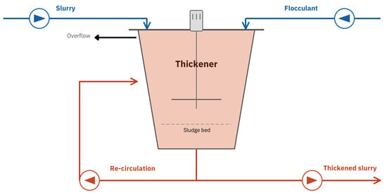
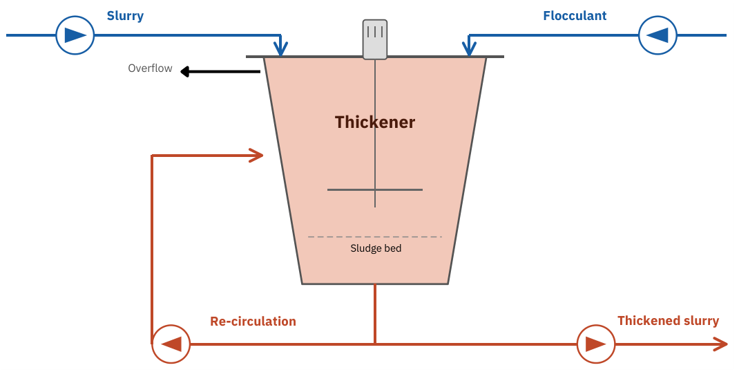
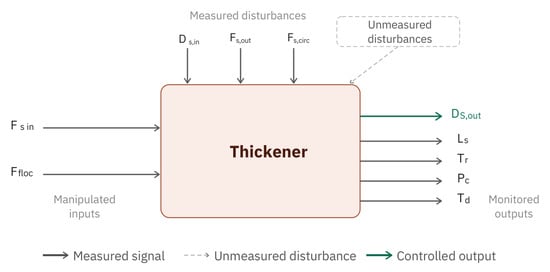
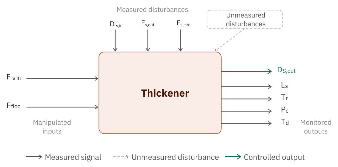
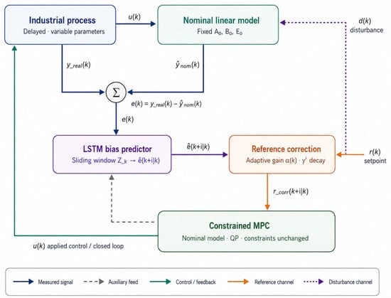
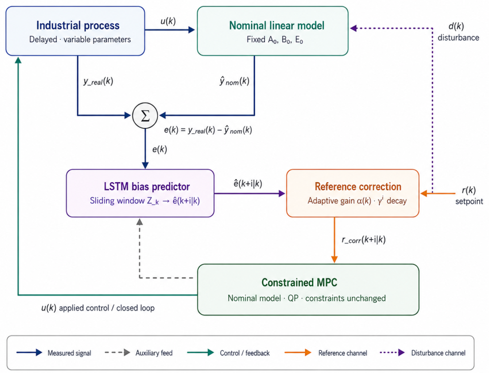
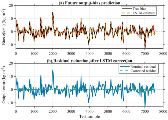
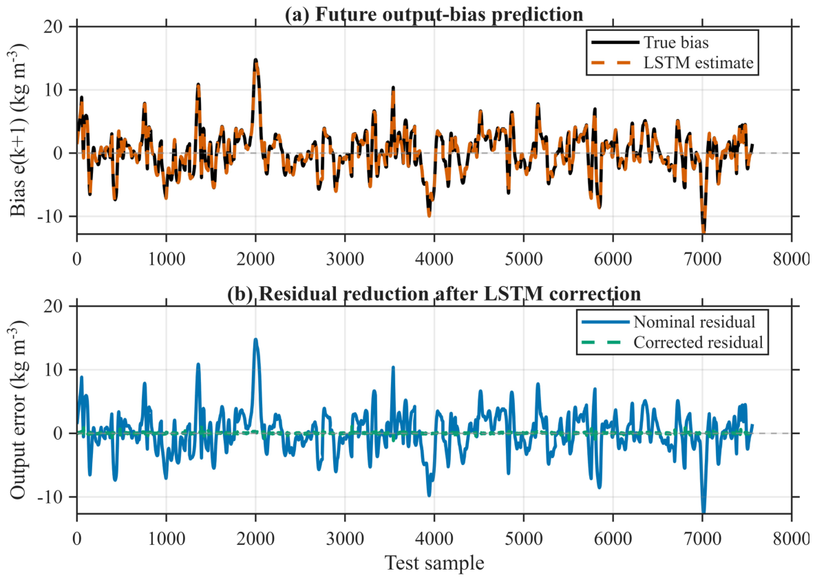
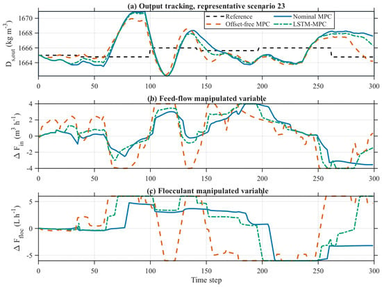
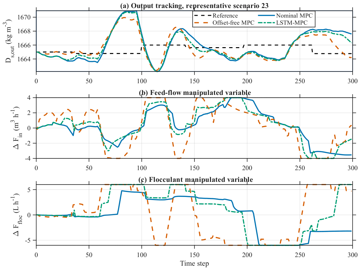
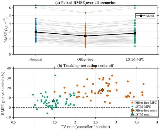
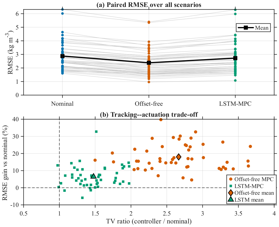

Disclaimer/Publisher’s Note: The statements, opinions and data contained in all publications are solely those of the individual author(s) and contributor(s) and not of MDPI and/or the editor(s). MDPI and/or the editor(s) disclaim responsibility for any injury to people or property resulting from any ideas, methods, instructions or products referred to in the content. |
© 2026 by the authors. Licensee MDPI, Basel, Switzerland. This article is an open access article distributed under the terms and conditions of the Creative Commons Attribution (CC BY) license.