Monocular 3D Tennis Serve Analysis and Rule-Based Feedback: System Design and Quasi-Experimental Validation

Abstract

This study aimed to develop a monocular vision-based tennis serve analysis system and evaluate its effectiveness in beginner training. The system uses MediaPipe Pose to extract 33 body landmarks from monocular video, calculates joint angles using three-dimensional vector operations, identifies serve phases through threshold-based rules, constructs an approximate 3D pose representation using anthropometric constraints, and generates corrective feedback through a rule-based expert system. In a quasi-experimental study, 90 beginner tennis players (final n = 82) completed an 8-week intervention and were allocated to a high-frequency feedback group, a moderate-frequency feedback group, or a conventional training group. All groups showed significant improvements in Serve Quality Mastery (SQM) scores (p < 0.001). The high-frequency feedback group showed the greatest SQM improvement (SQM: +30.5 points), followed by the moderate-frequency feedback group (+24.2 points) and the conventional training group (+15.5 points). Between-group differences were significant F(2, 79) = 74.30, p < 0.001, η² = 0.65. These findings indicate a graded pattern across the feedback-frequency groups, with more frequent system-generated feedback being associated with greater improvements in training performance. The findings support the potential use of the monocular pose-based, rule-driven feedback system as a supplementary tool for beginner tennis serve instruction.

1. Introduction

Tennis is a globally practiced sport with a broad and increasingly diverse participation base. According to recent international participation reports, worldwide tennis participation has continued to grow, reflecting the sport’s accessibility across recreational, educational, and competitive settings. Tennis players range from occasional recreational participants and school or university learners to trained amateur and professional athletes. This wide player profile creates a strong need for training methods that can support not only elite performance analysis but also beginner skill acquisition, especially in settings where access to expert coaching and advanced biomechanical equipment may be limited. Tennis is also a technically demanding sport in which competitive performance depends heavily on the correctness and consistency of stroke technique. A standardized stroke technique not only improves ball control and speed but also effectively prevents sports injuries [1]. From a bioenergetic perspective, tennis is an intermittent sport characterized by repeated short bursts of high-intensity effort interspersed with brief recovery periods. The tennis serve is an explosive movement that relies heavily on rapid force production through the kinetic chain, and its immediate energy demand is primarily supported by the phosphagen system and anaerobic metabolism. During repeated practice or match play, aerobic metabolism also plays an important role by supporting recovery between points, maintaining technical consistency, and delaying fatigue. The phosphagen-dominant nature of the serve, combined with the rapid recovery between individual serve attempts, makes repeated within-session practice physiologically feasible for beginner players. This also supports the value of between-trial corrective feedback: when motor patterns are not yet consolidated, timely and specific feedback provided during the recovery interval between serve attempts is more likely to influence the subsequent attempt than feedback delivered at the end of a session. Thus, effective serve training should consider not only biomechanical coordination but also the physiological demands associated with repeated explosive movement execution. However, tennis serves are highly complex and dynamic, involving coordinated movements of multiple joints throughout the body. Take the serve as an example: a complete serving motion requires precise coordination between the tosser and the server, coordinated rotation of the hips and shoulders, and a whipping motion of the arm—all of which place extremely high technical demands on the athlete [2]. Traditional tennis training relies heavily on coaches’ visual observation and subjective judgment, a model that has significant drawbacks. During training, a coach’s field of view is limited, making it impossible to fully capture all details of an athlete’s movements. Furthermore, constrained by the human eye’s resolution and reaction speed, it is difficult to accurately identify even minor deviations in an athlete’s form. Training effectiveness lacks a quantitative basis for evaluation, and assessment results are highly subjective. Athletes are also unable to receive real-time quantitative feedback on their movements, which hinders timely corrections [3].

With the rapid development of computer vision and artificial intelligence technologies, particularly the breakthroughs in deep learning for image recognition [4], it has become possible to use AI technology to assist in sports training. Human pose estimation (HPE) technology can automatically extract key point information of the human skeleton from images or videos, providing a data foundation for motion analysis [5]. By integrating biomechanical theory and expert knowledge, intelligent systems capable of automatically evaluating movement quality and providing improvement recommendations can be developed [6,7]. Human pose estimation is a classic problem in the field of computer vision, and significant progress has been made in recent years [8]. Early methods were primarily based on pictorial structures and deformable part models [9,10]; these approaches relied on manually designed feature extractors and had limited performance in complex scenes. In 2014, Toshev et al. first introduced deep learning into the field of human pose estimation by proposing the end-to-end DeepPose model [11]. Subsequently, a series of related models were introduced, such as Convolutional Pose Machines (CPM), Stacked Hourglass, OpenPose, and High-Resolution Networks (HRNet) [12,13,14,15,16]. Regarding 3D pose estimation, which leverages prior knowledge such as human anatomical and kinematic constraints to assist estimation [17,18], current mainstream monocular 3D methods include regression-based and reconstruction-based approaches [19,20,21]. However, due to depth ambiguity, the accuracy of monocular methods remains significantly lower than that of solutions based on multi-camera systems or depth sensors [22]. These methods have substantially improved the accuracy and robustness of pose estimation, laying the technical foundation for sports motion analysis [23,24,25,26]. While some existing commercial systems are powerful, they are often expensive and lack specific optimizations tailored to the characteristics of tennis [27,28].

Monocular 3D human pose estimation is commonly formulated as a 2D-to-3D pose-lifting problem, in which temporally ordered two-dimensional joint coordinates are mapped to three-dimensional pose sequences. VideoPose3D established an influential temporal-convolutional baseline by applying dilated temporal convolutions to 2D keypoint trajectories [29]. Subsequent transformer-based approaches placed greater emphasis on long-range spatial and temporal dependencies. PoseFormer separately models within-frame joint relationships and across-frame motion dynamics using spatial and temporal transformer modules [30], whereas MHFormer addresses monocular depth ambiguity by learning and integrating multiple plausible pose hypotheses [31]. MixSTE further improves sequence-level pose estimation by alternately modeling the spatial configuration of joints and the temporal trajectory of each joint [32]. More recent methods have extended this direction through large-scale motion pretraining and hybrid architectures. MotionBERT learns transferable human-motion representations by recovering underlying 3D motion from noisy or incomplete 2D observations [33], while PoseFormerV2 introduces frequency-domain representations to improve computational efficiency and robustness to noisy 2D detections [34]. MotionAGFormer combines transformer-based global modeling with graph-based local skeletal modeling to capture complementary spatial and temporal dependencies [35]. At the video-based 2D pose-estimation stage, DSTA decouples spatial relationships between adjacent joints from the temporal trajectory of each individual joint, providing an efficient strategy for obtaining more stable landmark sequences under motion blur and occlusion [36].

In sports biomechanics, pose estimation alone is insufficient unless the estimated landmarks can be translated into meaningful kinematic variables, technique assessments, and actionable feedback. Recent research has therefore increasingly connected markerless pose estimation with joint-angle analysis, movement-phase recognition, performance assessment, and coaching support. Sports-specific validation is particularly important because models trained on conventional human-pose datasets may not generalize reliably to rapid, high-acceleration athletic movements [37]. In tennis, recent studies have investigated spatiotemporal pose lifting for motion analysis [2], MediaPipe- and optical flow-based swing trajectory comparison [27], and multi-modal analysis of ball position, racket pose, and future trajectory through the Racket Vision benchmark [28]. Emerging explainable sports-analysis frameworks further seek to convert biomechanical and temporal motion features into interpretable diagnostic indicators and language-based training guidance rather than providing only a numerical score or a visually reconstructed pose. These developments indicate that practical sports-training systems must balance pose-estimation performance with computational accessibility, domain-specific biomechanical interpretation, and transparency of the generated recommendations.

Although recent temporal-convolutional, transformer-based, and hybrid architectures have achieved strong performance in monocular 3D human pose estimation, their use often requires task-specific model training, large-scale annotated datasets, higher computational resources, and offline sequence-level processing. These characteristics make them less suitable for the present study, which aims to develop an accessible, transparent, and practical feedback-support system for beginner tennis instruction rather than to advance state-of-the-art 3D pose-estimation accuracy. MediaPipe Pose was therefore selected because it provides real-time monocular landmark extraction, includes a dense set of 33 body landmarks, can be deployed with relatively low computational cost, and supports practical use in ordinary training environments without specialized motion-capture equipment. In this study, MediaPipe outputs are not treated as metrically accurate 3D joint positions; instead, they are used as accessible landmark inputs for approximate 3D pose representation, joint-angle calculation, serve-phase recognition, and rule-based feedback generation.

This study employs MediaPipe Pose [38] as the core pose estimation framework to develop a monocular tennis serve analysis and rule-based feedback system. The study extracts 33 body landmarks and uses three-dimensional vector angle calculation to obtain core joint angles; it divides the serve into phases based on temporal changes in joint angles while establishing a multidimensional movement-quality assessment framework. The study employs monocular vision combined with anthropometric constraints to construct an approximate 3D pose representation. By integrating biomechanical knowledge and professional expertise, a rule-based expert system is used to generate personalized corrective feedback, ultimately realizing an integrated application for the analysis, evaluation, and correction of tennis serve movements. Furthermore, this study uses a quasi-experimental design to evaluate whether different frequencies of system-generated feedback are associated with differences in serve performance and learning efficiency among beginner tennis players. Unlike data-driven 2D-to-3D lifting approaches such as VideoPose3D, MotionBERT, and MotionAGFormer, the present study does not propose or train a new 3D pose-estimation backbone. Its contribution lies in integrating an accessible pose-estimation framework with biomechanically interpretable measurements, transparent rule-based feedback, and a quasi-experimental evaluation of training outcomes.

2. Materials and Methods

2.1. Participants

This study recruited a total of 90 students enrolled in a tennis elective course at the School of Physical Education of a certain university as research subjects. None of the participants had previously received formal tennis training, had any prior tennis skills, were in good health, and had no history of physical injuries or cardiovascular or cerebrovascular diseases that would be associated with differences in their ability to exercise. All participants signed an informed consent form for the collection of training data prior to participation. Based on the intensity of the training intervention, the participants were divided into three groups: Experimental Group A underwent high-intensity system-assisted training with systematic analysis conducted four times per week; Experimental Group B underwent moderate-intensity system-assisted training with systematic analysis conducted twice per week; and the Control Group underwent conventional training using a traditional teaching model. The primary objective of establishing different intervention intensities was to investigate the impact of the system’s usage frequency on training outcomes. The experimental period lasted 8 weeks, with all groups scheduled for two training sessions per week, each lasting 90 min. All groups followed a standardized training curriculum, differing only in training methodology. Both experimental groups adopted a combined “conventional training + system-assisted analysis” model, comprising a 15 min warm-up, 30 min of fundamental skill practice, 15 min of competitive drills, and 30 min of system-assisted analysis. The control group followed the traditional “coach demonstration–student imitation–coach correction” training model, without the use of any system-generated feedback tools. Exclusion criteria included voluntary withdrawal, absence from more than 20% of total training sessions, or inability to complete all tests and training due to injury or illness.

2.2. Experimental Design

This experiment aims to systematically validate the practical value of a monocular pose-based tennis serve analysis system and to clarify its role in improving the quality of learners’ strokes. The study employed a pre-post test design with unequal groups within a quasi-experimental design, comprising three groups of 30 participants each. The specific grouping scheme is shown in

Table 1. Experimental Grouping Scheme.

Group	Number of Participants	Training Method	Intensity of Intervention
Experimental Group A	30	Conventional training + system-assisted analysis	High intensity (systematic analysis 4 times per week)
Experimental Group B	30	Conventional training + pose-based feedback	Moderate intensity (systematic analysis 2 times per week)
Control Group	30	Conventional training	Traditional instruction, no system-generated feedback tools

:

All participants were students enrolled in an elective tennis course at the School of Physical Education of a certain university. None had prior tennis experience, and all met the inclusion criteria. The baseline characteristics (age, height, and gender ratio) were balanced across the three groups to ensure the validity of the grouping. The study lasted 8 weeks, with each group scheduled for two 90 min training sessions per week. All groups followed a standardized training curriculum, differing only in training methods: the experimental group incorporated system-assisted analysis into some of their weekly training sessions, while the control group adhered to a traditional training model throughout. The groups differed in the availability and frequency of system-generated feedback rather than in the number of formal training sessions. The specific arrangements are shown in

Table 2. Weekly Training Content and Focus Areas.

Week	Training Content	Key Techniques
Weeks 1–2	Racket grip, ready position, ball feel drills and basic serve preparation	Basic stance and continental grip, ready posture, and serve preparation
Weeks 3–4	Serve toss drills without ball striking and segmented serve-practice drills	Toss-arm elevation, stable ball release, shoulder alignment, and preparation-to-toss transition
Weeks 5–6	Basic complete serve drills and serve-phase coordination practice	Backswing coordination, arm extension at impact, contact-point control, and trunk inclination control
Weeks 7–8	Consolidated complete serve practice and feedback-based correction	Serve rhythm, follow-through completion, movement stability, and consistency of serve execution

:

Methods for Experimental Data Collection and Processing

This experiment data included demographic characteristics, serve-performance scores, coach-rated movement assessment scores, and training efficiency indicators. Demographic variables included age, height, weight, and gender. Serve performance was assessed using the Serve Quality Mastery (SQM) score, while movement quality was additionally evaluated by three professional tennis coaches using the Movement Assessment Criteria (MAC). Training efficiency indicators included the time required to reach the predefined SQM and MAC thresholds. All data were checked for completeness before statistical analysis. The statistical procedures are described separately in Section 2.4.

The equipment and tools used for participant evaluation included anthropometric measurement tools, monocular video-recording equipment, the proposed pose-analysis system, standardized coach-rating forms, and statistical analysis software. Body height and body weight were measured using a stadiometer and an electronic weighing scale, respectively. Tennis serve movements were recorded using a monocular video camera or smartphone camera mounted on a tripod at a fixed position relative to the serving area. The same recording setup was used throughout the intervention to reduce variation caused by camera position or viewing angle. Coach-rated Movement Assessment Criteria (MAC) scores were recorded using standardized rating forms completed independently by three professional tennis coaches. Statistical analyses were performed using SPSS (version 26.0).

2.3. System Architecture

The system developed in this study consists of four core modules: pose estimation, movement-quality assessment, approximate 3D pose representation, and rule-based feedback generation. The system processes the input video through stages such as pose detection, keypoint extraction, joint angle calculation, motion phase recognition, quality scoring, and approximate 3D pose representation, ultimately generating personalized improvement recommendations.

2.3.1. Pose Estimation Model

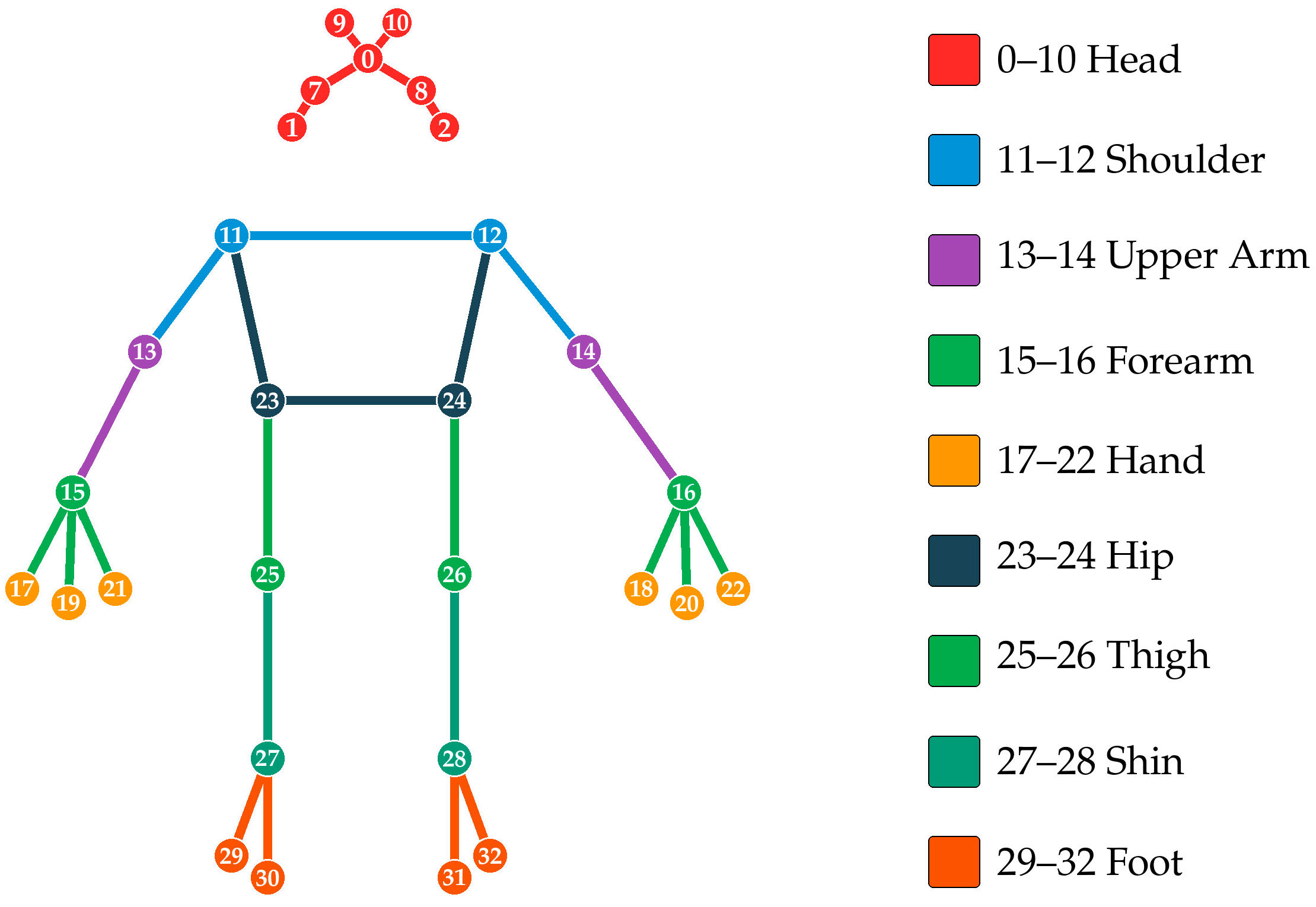
This study uses the MediaPipe Pose framework, which defines body landmarks covering all major regions of the head, torso, upper limbs, and lower limbs. The position of each landmark is represented by normalized image coordinates, a model-estimated relative-depth component, and a visibility score:

$$P_i=\left(x_i,y_i,z_i,v_i\right)$$

(1)

Here, $x_i$ and $y_i$ represent normalized image coordinates (with values ranging from [0, 1]), and $z_i$ represents the model-estimated relative-depth component, with the midpoint of the left and right hips as the origin, indicating the anterior–posterior displacement of the keypoint relative to the hip plane. Additionally, each keypoint includes a visibility score ${\mathrm{v}}_{\mathrm{i}}$, which represents the model’s confidence in detecting that keypoint, with values ranging from [0, 1]. The z-value is not a metrically calibrated camera-to-subject depth measurement, and the resulting landmark coordinates should not be interpreted as absolute three-dimensional joint positions. Instead, these outputs are used to construct an approximate 3D pose representation for subsequent joint-angle calculation, movement-phase recognition, and rule-based feedback generation.

Skeletal connections define the topological relationships between landmarks, forming a structural graph of the human skeleton. By defining 12 primary skeletal connections, the resulting graph is used for pose visualization and structural analysis, as shown in

Table 3. Skeletal Connection Table.

Number	Start	End	Bone Name	Anatomical Significance
1	11 (Left Shoulder)	12 (Right Shoulder)	Clavicle	Transverse line of the shoulder
2	11 (Left Shoulder)	13 (Left Elbow)	Left Upper Arm	From the left shoulder joint to the left elbow joint
3	13 (Left Elbow)	15 (Left Wrist)	Left Forearm	Left Elbow Joint to Left Wrist Joint
4	12 (Right Shoulder)	14 (Right Elbow)	Right Upper Arm	Right Shoulder Joint to Right Elbow Joint
5	14 (Right Elbow)	16 (Right Wrist)	Right Forearm	Right Elbow Joint to Right Wrist Joint
6	11 (Left Shoulder)	23 (Left Hip)	Left Trunk	From left shoulder to left hip
7	12 (Right Shoulder)	24 (Right Hip)	Right Trunk	From right shoulder to right hip
8	23 (Left Hip)	24 (Right hip)	Pelvis	Horizontal line at the hip
9	23 (Left Hip)	25 (Left knee)	Left thigh	From the left hip joint to the left knee joint
10	25 (Left knee)	27 (Left Ankle)	Left Lower Leg	From Left Knee to Left Ankle
11	24 (Right hip)	26 (Right Knee)	Right Thigh	From Right Hip to Right Knee
12	26 (Right Knee)	28 (Right Ankle)	Right Lower Leg	From Right Knee to Right Ankle

.

The topological structure of the human skeleton can be modeled using undirected graphs.

$$G=\left(V,E\right)$$

(2)

Here, $V = 0,1,2,...,32$ contains a total of 33 vertices, corresponding to the 33 key points of the human body, and $\mathrm{E}$ is the set of skeletal edges, containing 12 undirected edges, each of which represents the skeletal connection between adjacent key points. Any skeletal edge is defined as $e = i$, $j\in E$, indicating that key point $i$ is skeletally connected to key point $\mathrm{j}$, and the undirected edge satisfies the equivalence of $i$, $j$ and $j$, $i$ as shown in Figure 1.

2.3.2. Coordinate Systems and Data Preprocessing

To facilitate human pose modeling and mathematical quantification, three types of coordinate systems are used for keypoint representation and operations: the original pixel coordinate system, where the origin is located at the top-left corner of the image, with the positive x-axis extending horizontally to the right and the positive y-axis extending vertically downward. By mapping image pixel coordinates to the interval [0, 1], scale differences caused by varying image resolutions are eliminated, enabling cross-scene pose analysis. Formula for converting pixel coordinates to normalized coordinates.

$$\begin{array}{c}{x}_{norm}={\displaystyle \frac{x_{pixel}}{W_{image}}}\\ y_{norm}={\displaystyle \frac{y_{pixel}}{H_{image}}}\end{array}$$

(3)

Here, $W_{\mathit{image}}$ and $H_{\mathit{image}}$ represent the width and height of the image, respectively. The method for calculating the local coordinate system of the torso uses the center of the torso as the origin, which is used for quantitative analysis of torso posture rotation and relative motion relationships. The center of the torso is obtained by taking the average of the midpoints of the left and right shoulders and the midpoints of the left and right hips, as shown in Equation (4).

$$P_{torso\_center}={\displaystyle \frac{1}{2}}\left({\displaystyle \frac{p_{11}+p_{12}}{2}}+{\displaystyle \frac{p_{23}+p_{24}}{2}}\right)$$

(4)

2.3.3. Joint-Angle Calculation Using Three-Dimensional Vector Angles

Joint angles are a core metric for evaluating pose quality. Given three points A, B, and C in space, where B is the joint vertex (i.e., the vertex of the angle), $\angle \mathrm{ABC}$ can be calculated using the vector angle formula. The three points are represented by their three-dimensional coordinate vectors as follows: $\overrightarrow{\mathrm{A}} = \left({\mathrm{x}}_{\mathrm{A}},{\mathrm{y}}_{\mathrm{A}},{\mathrm{z}}_{\mathrm{A}}\right)$; $\overrightarrow{\mathrm{B}} = \left({\mathrm{x}}_{\mathrm{B}},{\mathrm{y}}_{\mathrm{B}},{\mathrm{z}}_{\mathrm{B}}\right)$; $\overrightarrow{\mathrm{C} }= \left({\mathrm{x}}_{\mathrm{C}},{\mathrm{y}}_{\mathrm{C}},{\mathrm{z}}_{\mathrm{C}}\right)$. Constructing the spatial vectors $\overrightarrow{\mathit{BA}}$ and $\overrightarrow{\mathit{BC}}$ with vertex B as the origin, and defining $\overrightarrow{\mathit{BA}}·\overrightarrow{\mathit{BC}} = ‖\overrightarrow{\mathit{BA}}‖‖\overrightarrow{\mathit{BC}}‖\cos \theta$ based on the dot product of spatial vectors, we obtain Equation (5).

$$\cos \theta ={\displaystyle \frac{\overrightarrow{\mathrm{BA}}·\overrightarrow{\mathrm{BC}}}{‖\overrightarrow{\mathrm{BA}}‖‖\overrightarrow{\mathrm{BC}}‖}}$$

(5)

Substituting the 3D coordinate components into the expansion yields the general formula for joint Equation (6).

$$\theta =\arccos \left({\displaystyle \frac{\left(x_A-x_B\right)\left(x_C-x_B\right)+\left(y_A-y_B\right)\left(y_C-y_B\right)+\left(z_A-z_B\right)\left(z_C-z_B\right)}{\sqrt{{\left(x_A-x_B\right)}^2+{\left(y_A-y_B\right)}^2+{\left(z_A-z_B\right)}^2}\cdot \sqrt{{\left(x_C-x_B\right)}^2+{\left(y_C-y_B\right)}^2+{\left(z_C-z_B\right)}^2}}}\right)$$

(6)

Due to floating-point calculation errors during the pose estimation process, the value of $\mathit{cos}\theta$ can easily exceed the domain of the inverse cosine function, which is −1 to 1. Therefore, by imposing a range constraint on the cosine value, we obtain Equation (7).

$$\cos {\theta }_{clamped}=\mathit{min}\left(1,\mathit{max}\left(-1,\mathit{cos}\theta \right)\right)$$

(7)

This paper selects two representative types of core joint angles in human motion and posture assessment for quantitative modeling. By combining these with the index coordinates of human key points, it establishes standardized definitions and solutions for each joint angle based on the aforementioned three-dimensional vector angle model.

The first category involves the calculation of joint angles in the limbs. Taking the right shoulder joint angle as an example, this angle represents the spatial angle between the right upper arm and the torso, and quantitatively reflects the range of motion of the right upper limb. The calculation utilizes the left hip keypoint ${\mathrm{P}}_{23}$, the right shoulder keypoint $P_{12}$, and the left shoulder keypoint ${\mathrm{P}}_{11}$. The formula is as follows:

$${\theta }_{r\_\mathrm{s}\mathrm{h}\mathit{oulder}} = \mathit{arccos}\left({\displaystyle \frac{\overrightarrow{P_{23}{P}_{12}}\cdot \overrightarrow{P_{23}{P}_{11}}}{‖\overrightarrow{P_{23}{P}_{12}}‖‖\overrightarrow{P_{23}{P}_{11}}‖}}\right)$$

(8)

The second category is trunk tilt angle, which represents the angle of deviation between the trunk’s central axis and the vertical direction. It is used to quantify the degree of forward, backward, and lateral tilt of the human trunk. First, the center points of the shoulders and hips are determined separately using the key points at the left and right shoulders and hips.

$$\begin{array}{c}{P}_{should\_centerP}={\displaystyle \frac{P_{11}+P_{12}}{2}}\\ P_{hip\_center}={\displaystyle \frac{P_{23}+P_{24}}{2}}\end{array}$$

(9)

Construct the reference vectors $\overrightarrow{{\mathrm{P}}_{\mathrm{hip}\_\mathrm{center}}{\mathrm{P}}_{\mathrm{shoulder}\_\mathrm{center}}}$. In the normalized image coordinate system, define the vertical upward reference vector as $\overrightarrow{{\mathrm{V}}_{\mathrm{up}}} = \left(0,-1,0\right)$, and solve for the trunk reference angle using the vector angle model.

$${\theta }_{\mathit{torso}}= \mathit{arccos}\left({\displaystyle \frac{\overrightarrow{V_{\mathit{up}}}\cdot \overrightarrow{P_{\mathrm{h}\mathit{ip}\_\mathit{center}}{P}_{s\mathrm{h}\mathit{oulder}\_\mathit{center}}}}{‖\overrightarrow{V_{\mathit{up}}}‖‖\overrightarrow{P_{\mathrm{h}\mathit{ip}\_\mathit{center}}{P}_{s\mathrm{h}\mathit{oulder}\_\mathit{center}}}‖}}\right)$$

(10)

To ensure the results of the actual pose estimation are both intuitive and physically meaningful, the arctangent function is used to optimize the solution for the trunk tilt angle. Let

$$\left\{\begin{array}{c}\Delta x=P_{s\mathrm{h}\mathit{oulder}\_\mathit{center}}\cdot x-P_{\mathrm{h}\mathit{ip}\_\mathit{center}}\cdot x\\ \Delta y=P_{\mathrm{h}\mathit{ip}\_\mathit{center}}\cdot y-{\mathrm{P}}_{s\mathrm{h}\mathit{oulder}\_\mathit{center}}\cdot y\end{array}\right.$$

(11)

then the trunk tilt angle can be expressed as:

$${\theta }_{\mathit{torso}\_\mathit{inclination}} = 90°-\mathit{arctan}2\left(\Delta y,\left|\Delta x\right|\right)$$

(12)

2.3.4. Action-Phase Recognition Algorithm

The tennis serve is a sequential process, and accurately identifying its phases is a prerequisite for targeted analysis. This section presents a phase recognition algorithm based on joint angle threshold rules. Taking the tennis serve as an example, a complete tennis serve can be broken down into the following five phases as shown in

Table 4. Movement Phases Table.

Phase	Phase Number	Key Characteristics	Estimated Duration
Preparation	1	Ball-holding hand hangs down, body upright, center of gravity stable	0.5–1.0 s
Toss	2	Non-ball-holding hand tosses the ball upward, arm extended	0.3–0.5 s
Backswing	3	Dominant hand raised backward and upward, elbow bent	0.5–1.0 s
Impact	4	Arm extended to strike the ball, body leaning forward	0.02–0.05 s
Follow-through	5	Arm drops naturally, body turns	0.5–1.0 s

.

Motion phase recognition is based on changes in key joint angles. This system employs a threshold-based method, setting a series of angle thresholds to determine the current phase of the motion. Let ${\theta }_{\mathrm{r}\_\mathrm{elbow}}$ denote the angle of the right elbow joint and ${\theta }_{\mathrm{r}\_\mathrm{shoulder}}$ denote the angle of the right shoulder joint. The phase determination rules are defined as follows:

$$phase\left(f\right)=\left\{\begin{array}{c}preparation if {\theta }_{r\_elbow}>150°\\ toss if if {\theta }_{r\_elbow}<150° and {\theta }_{r\_shoulder}<45°\\ \begin{array}{c}backswing if {45°\le \theta }_{r\_shoulder}<90°\\ impact if {\theta }_{r\_shoulder}\ge 90° and {\theta }_{r\_elbow}\ge 100°\\ followthrough if {\theta }_{r\_shoulder}\ge 90° and {\theta }_{r\_elbow}<100°\end{array}\end{array}\right.$$

(13)

The thresholds were determined based on preliminary experimental data from 10 amateur tennis players (aged 20–25, height 165–180 cm). Twenty serve motions were recorded for each player, and initial thresholds were set by analyzing the statistical characteristics (mean ± standard deviation) of joint angle distributions. These thresholds were then fine-tuned following manual annotation and verification by three tennis coaches. These threshold rules apply to standard right-handed serve techniques; left-handed players should apply a mirror-image adjustment.

2.3.5. Preliminary Rule-Based Serve Feedback Index

The system uses a preliminary rule-based index to convert selected kinematic features into structured and interpretable instructional feedback. The index is intended to support feedback generation and should not be interpreted as a fully validated biomechanical or psychometric measure of overall tennis serve quality.

The index includes four observable components derived from the available landmark and phase-recognition outputs: toss-arm elevation, arm extension, trunk inclination, and follow-through duration. These components represent selected aspects of the tennis serve rather than the complete kinetic chain as shown in

Table 5. Serve Motion Evaluation Indicators.

Name	Description	Max Score
Toss-Arm Elevation	Evaluates shoulder elevation during the ball-toss phase	100
Arm Extension	Evaluates elbow extension during the impact phase	100
Trunk Inclination	Evaluates whether trunk inclination during the backswing remains within a predefined phase-specific reference range	100
Follow-through Duration	Evaluates the duration of the recognized follow-through phase	100

.

The scores for each sub-indicator are combined using a weighted sum, resulting in a final composite score for the serve.

$${\mathrm{Score}}_{\mathit{overall}}={\displaystyle \frac{w_1\cdot S_{\mathit{toss}}+w_2\cdot S_{\mathit{extension}}+w_3\cdot S_{\mathit{rotation}}+w_4\cdot S_{\mathit{follow}}}{w_1+w_2+w_3+w_4}}$$

(14)

In the formula, ${\mathrm{S}}_{\mathrm{toss}},{ \mathrm{S}}_{\mathrm{extension}}, {\mathrm{S}}_{\mathrm{rotation}}, {\mathrm{S}}_{\mathrm{follow}}$ represent the component scores for toss-arm elevation, arm extension, trunk inclination, and follow-through duration, respectively; The corresponding weights $w_1,w_2,w_3,w_4$ are the weighting coefficients for the corresponding metrics. This paper adopts an equal-weighting evaluation model by default. Specifically, each component was assigned a weight of 0.25. Equal weighting was adopted because the four components represent different phases and technical characteristics of the tennis serve, and no prior empirical evidence was available to justify assigning greater importance to any single component. This neutral weighting strategy also avoids introducing additional subjective preference into the composite score. The equal weights should therefore be understood as a transparent rule-based design choice rather than as evidence that the four components have identical biomechanical importance.

(1) Ball Release Control Score

The ball release control score is calculated based on the average angle of the right shoulder joint during the ball release phase, as shown in the following formula:

$$S_{\mathit{toss}} = 100\max \left(0,\min \left(1,1-{\displaystyle \frac{{\mathrm{d}}_{\mathrm{toss}}}{{\tau }_{\mathrm{toss}}}}\right)\right)$$

(15)

In the formula, ${\stackrel{\mathrm{̄}}{\theta }}_{\mathrm{r}\_\mathrm{shoulder}}$ represents the average angle of the right shoulder joint during the ball-toss phase; ${\alpha }_{\mathrm{toss}}$ is a scaling factor, which is set to 1.5 based on the standard ball-toss posture (where the angle of the ball-holding shoulder ranges from 120° to 140°); the maximum score is 100 points. The original coefficient $\alpha =1.5$ was removed because the original formulation caused scores within the stated shoulder-angle range to saturate at 100. The revised rule assigns the maximum score within a predefined reference interval and progressively reduces the score outside that interval.

(2) Arm Extension Score

The arm extension score is determined based on the average angle of the right elbow joint during the swing phase, as shown in the following formula:

$$S_{\mathit{extension}} = \max \left(0,\min \left(100,100-{\beta }_{\mathrm{ext}}\left|180°-{\theta }_{\mathrm{e}\mathrm{l}\mathrm{b}\mathrm{o}\mathrm{w}}\right|\right)\right)$$

(16)

In the formula, ${\stackrel{\mathrm{̄}}{\theta }}_{\mathrm{r}\_\mathrm{elbow}}$ represents the average angle of the right elbow joint during the swing phase; ${\beta }_{\mathrm{ext}}$ is the extension correction factor, set to ${\beta }_{\mathrm{ext}} = 2.0$; the closer the elbow joint is to 180° (fully extended), the closer the score is to 100 points. The value ${\beta }_{\mathrm{e}\mathrm{x}\mathrm{t}}=2.0$ was used as a deviation penalty, such that each degree of deviation from the target extension angle reduces the component score by two points.

(3) Trunk Inclination Score

The available landmark-based variable represents trunk inclination relative to the vertical direction rather than axial hip–shoulder rotation. Therefore, this component was renamed the “trunk inclination score.” The original formulation increased the score as the trunk angle deviated further from $\left(90^{\circ }\right)$, which could incorrectly reward excessive inclination. The revised formulation assigns the highest score when the measured trunk angle falls within a predefined phase-specific reference interval and progressively reduces the score when the angle falls outside this interval:

$$S_{\mathit{trunk}} = 100·\max \left(0,\min \left(1,1-{\displaystyle \frac{\max \left({\theta }_{\mathrm{L}}-{\theta }_{\mathrm{t}\mathrm{o}\mathrm{r}\mathrm{s}\mathrm{o}},0,{\theta }_{\mathrm{t}\mathrm{o}\mathrm{r}\mathrm{s}\mathrm{o}}-{\theta }_{\mathrm{U}}\right)}{{\tau }_{\mathrm{trunk}}}}\right)\right)$$

(17)

Here, ${\theta }_{torso}$ represents the average trunk inclination angle during the backswing phase; $[{\theta }_L,{\theta }_U]$ is the acceptable phase-specific reference interval; and ${\tau }_{trunk}$ is the maximum tolerated deviation outside that interval. The distance function is zero when the measured angle lies within the reference interval and increases according to the distance from the nearest boundary when the angle lies outside the interval. Thus, the revised formula does not assume that a larger angular deviation represents better biomechanical performance. The original coefficient ${\gamma }_{rot}=1.0$ and the monotonic deviation-based scoring rule were removed.

(4) Follow-Through Completeness Score

The follow-through completeness score is quantified based on the number of frames in the follow-through phase, as shown in the following formula:

$$S_{\mathit{follow}} = \min \left(100,{\delta }_{\mathit{follow}}\cdot N_{\mathit{follow}}\right)$$

(18)

In the formula, $N_{\mathit{follow}}$ represents the number of frames in the follow-along phase; ${\delta }_{\mathrm{follow}}$ represents the weighting factor for a single frame. To meet the requirement for a complete follow-along (no fewer than 10 frames), ${\delta }_{\mathit{follow}}$ is set to 10; the maximum score is 100 points. The value ($\delta$ = 10) was selected because a complete follow-through was operationally defined as lasting at least 10 frames under the standardized video-recording conditions used in this study. Accordingly, each valid follow-through frame contributed 10 points, and 10 or more frames corresponded to the maximum score of 100. This parameter is specific to the fixed recording frame rate used in the present study and may require recalibration when other frame rates are used.

These coefficients were introduced as transparent heuristic parameters for instructional feedback rather than as universally validated biomechanical constants. Their external validity and optimal values should be examined in future studies using larger samples, structured expert evaluation, and comparisons with validated biomechanical or coaching assessments.

2.3.6. Provisional Feedback Categories

To achieve quantitative evaluation and classification of motion quality, based on the comprehensive score results described above, this system classifies motion quality into four grades. The specific criteria for each grade are shown in

Table 6. Motion Quality Classification Table.

Name	Score Range	Color	Description
Excellent	90–100	Green	The technique is standard and meets professional standards
Good	75–89	Blue	The technique is generally standard, with some room for improvement
Fair	60–74	Yellow	Significant issues are present; focused practice is needed
Poor	0–59	Red	Serious issues are present; it is recommended to start from the basics

.

2.3.7. Approximate 3D Pose Representation Using Anthropometric Constraints

Monocular video does not directly provide metrically calibrated depth information, and a single two-dimensional landmark may correspond to multiple possible positions in three-dimensional space. Therefore, the method used in this study does not claim to recover absolute three-dimensional joint positions. Instead, MediaPipe relative-depth estimates are combined with anthropometric constraints to construct an approximate 3D pose representation for movement visualization, joint-angle calculation, movement-quality assessment, and rule-based feedback generation. This system employs a height-based proportional estimation method to obtain an approximate relative-depth representation, using each participant’s measured body height ${\mathrm{H}}_{\mathrm{i}}$ as the scaling reference. It combines this with the principle of similar triangles to estimate an approximately scaled depth value. Let the image height be ${\mathrm{H}}_{\mathrm{image}}$, the normalized height ratio of the human body in the image be $h$ and the effective focal-length parameter $\mathrm{f}$ be approximated as half of the image width, and the measured height of participant $\mathrm{i}$ be ${\mathrm{H}}_{\mathrm{i}}$. Then, the formula for calculating depth $D_i$ is:

$$D_i = {\displaystyle \frac{f\cdot H_i}{h\cdot H_{\mathit{image}}}}$$

(19)

In a normalized coordinate system, this can be simplified to $D_i=k_i/h$, where $k_i$ is a participant-specific scaling constant determined by the measured height of participant $i$. Thus, the revised procedure no longer assumes a fixed height of 1.7 m for all participants.

A sensitivity analysis was also added to evaluate the potential error introduced by the previous fixed-height assumption. Because the estimated depth is linearly proportional to the assumed height, the relative scaling error can be approximated as:

$${\displaystyle \frac{H_{\mathrm{r}\mathrm{e}\mathrm{f}}-H_i}{H_i}}\times 100\%$$

(20)

The method uses each participant’s measured height to reduce systematic scaling bias.

The lengths of various parts of the human skeleton have relatively fixed proportional relationships, which serve as anthropometric regularization constraints for constructing the approximate 3D pose representation. The anthropometric constraints used in this study are based on classical human body segment parameter models. In these models, the human body is represented as a linked system of anatomical segments, and segment dimensions can be expressed as proportions of total body height. The representative segment-length proportions adopted in this study were determined with reference to established anthropometric studies on body segment properties and segment parameter adjustment [38,39]. The standard skeletal proportion parameters adopted by this system are shown in

Table 7. Standard Skeletal Proportion Parameters [39].

Name	Proportion Relative to Height	Typical Length (for a Person 1.7 m Tall)
Head + Neck	0.14	0.238m
Torso	0.30	0.510m
Upper Arm	0.18	0.306m
Forearm	0.15	0.255m
Hand	0.05	0.085m
Thigh	0.25	0.425m
Shin	0.25	0.425m
Foot	0.05	0.085m

.

In addition, the proportions of adjacent bone segments are consistent (e.g., upper arm: forearm: hand ≈ 1:0.85:0.28, thigh: lower leg ≈ 1:1), which can serve as auxiliary constraints.

Based on the approximate relative-depth values and two-dimensional landmark coordinates, an approximately scaled pose representation is constructed through coordinate mapping.

$$\left\{\begin{array}{c}{x}_i^{3D}=\left(x_i^{2D}-0.5\right)\cdot D\cdot {\mathit{scale}}_x\\ y_i^{3D}=\left(0.5-y_i^{2D}\right)\cdot D\cdot {\mathit{scale}}_y\\ z_i^{3D}=z_i^{\mathit{relative}}\cdot D\end{array}\right.$$

(21)

Here, $\mathrm{D}$ represents the approximately scaled relative-depth value, ${\mathrm{scale}}_{\mathrm{x}}$ and ${\mathrm{scale}}_{\mathrm{y}}$ are coordinate scaling factors, and ${\mathrm{z}}_{\mathrm{i}}^{\mathrm{relative}}$ is the relative depth value output by the pose estimation model. The mapped coordinates are used as an internally consistent approximate pose representation and are not expressed in a validated global metric coordinate system. To reduce anatomically implausible variations in the approximate pose representation, the preliminary coordinates are regularized using skeletal length constraints. Let the expected length of the bone joint $\left(i, j\right)$ be $L_{\mathit{ij}}$ (determined based on human proportions), and the current estimated length be ${\overline{\mathrm{L}}}_{\mathrm{ij}}$. Then, the scaling factor is ${\lambda }_{\mathrm{ij}} = {\displaystyle \frac{{\mathrm{L}}_{\mathrm{ij}}}{{\overline{\mathrm{L}}}_{\mathrm{ij}}}}$. By adjusting the coordinates at both ends of the bone based on the scaling factor, we obtain the following formula:

$$\left\{\begin{array}{c}{P}_i^{\mathit{new}} = P_{\mathit{center}}+\left({P_i-P}_{\mathit{center}}\right)\cdot {\lambda }_{\mathit{ij}}\\ P_j^{\mathit{new}} = P_{\mathit{center}}+\left({P_j-P}_{\mathit{center}}\right)\cdot {\lambda }_{\mathit{ij}}\end{array}\right.$$

(22)

Here, ${\mathrm{P}}_{\mathrm{center}} = {\displaystyle \frac{{\mathrm{P}}_{\mathrm{i}}+{\mathrm{P}}_{\mathrm{j}}}{2}}$ represents the coordinates of the midpoint of the bone segment. The desired length parameters for the core bone joints in this system are shown in

Table 8. Desired Lengths of Bone Joints [40].

Skeletal Joints	Index Pairs	Expected Length (Relative to Height)
Shoulder Width	(11, 12)	0.30
Left Upper Arm	(11, 13)	0.18
Left Forearm	(13, 15)	0.15
Right Upper Arm	(12, 14)	0.18
Right Forearm	(14, 16)	0.15
Left Thigh	(23, 25)	0.25
Left Calf	(25, 27)	0.25
Right Thigh	(24, 26)	0.25
Right Calf	(26, 28)	0.25

:

After anthropometric regularization, joint angles are calculated from the approximately scaled landmark coordinates for subsequent pose quality assessment. The anthropometric constraints reduce anatomically implausible variations and improve the internal consistency of the estimated pose; however, monocular pose estimation remains an ill-posed problem because depth ambiguity cannot be fully resolved from a single camera view. These constraints reduce the possible solution space, but they do not produce a unique or metrically accurate three-dimensional reconstruction. Because synchronized marker-based motion-capture data or calibrated multi-camera ground-truth data were not collected, MPJPE, P-MPJPE, PCK, and metric 3D joint-position errors could not be reliably calculated. The resulting output should therefore be interpreted as an approximate 3D pose representation used within the proposed movement-analysis and rule-based feedback framework.

2.3.8. Rule-Based Feedback Generation Method

To provide targeted guidance for tennis serve movements, a rule-based feedback generation module was designed based on the preliminary serve feedback index. This module employs an IF–THEN rule engine that combines biomechanical principles with specialized tennis-coaching expertise to construct a feedback-rule library. This design enables the rule-based identification of movement issues and the automatic generation of corrective recommendations. The rule-based feedback library is the core of the feedback generation module. Each rule consists of a trigger condition and corresponding recommendation content designed specifically for the tennis serve. The feedback rules for the serve are organized around four core elements: toss-arm elevation, arm extension, trunk inclination, and follow-through duration. The specific rules are shown in

Table 9. Feedback rules for the Tennis Serve.

Rule ID	Trigger Conditions	Recommendations
TR-01	Toss-arm elevation score < 70	It is recommended to practice a consistent toss motion, keeping the ball at eye level—ideally about 30 cm in front of the body and at a height of approximately 1.8 to 2.0 m.
TR-02	Arm extension score < 70	At the moment of contact, the arm should be fully extended to create a “whipping” effect, thereby increasing power and speed; it is recommended to strengthen the shoulders and core muscles through strength training to enhance the stability of the arm extension.
TR-03	Trunk inclination score < 60	Review trunk alignment during the backswing and avoid excessive forward, backward, or lateral inclination. Hip–shoulder rotation should be assessed separately because it is not directly quantified by the current trunk-inclination measure.
TR-04	Follow-through duration score < 50	The follow-through should be complete and natural; after striking the ball, the arm should fall to the left side of the body or behind it to ensure full release of power while improving accuracy in controlling the landing point.
TR-05	Otherwise	The overall serve technique is solid. It is recommended to maintain the current training routine while focusing on improving movement consistency.

.

This module should be interpreted as a transparent rule-based recommendation engine rather than a machine learning-based, reinforcement-learning-based, LLM-based, or adaptive recommendation model.

2.4. Sample Size Calculation

A priori sample size calculation was conducted for the planned between-group comparison of the three training groups. The primary outcome was the Serve Quality Mastery (SQM) score. Assuming a one-way analysis of variance with three groups, a significance level of (alpha = 0.05), statistical power of 0.80, and a large expected effect size of (f = 0.40) was selected. This effect size was selected based on comparable pose-based sports-feedback interventions reporting between-group Cohen’s f values in the range of 0.38–0.45 for serve-performance outcomes under different feedback-frequency conditions. Under these assumptions, the minimum required sample size was estimated to be approximately 66 participants, corresponding to 22 participants per group. Considering possible attrition during the 8-week intervention, 90 participants were initially recruited, with 30 participants assigned to each group. After attrition, 82 participants completed the study and were included in the final analysis, which remained above the minimum required sample size.

2.5. Statistical Analysis

All statistical analyses were performed using SPSS. Continuous variables were expressed as mean ± standard deviation, and categorical variables were expressed as frequencies and percentages. Data completeness was checked before analysis.

The Shapiro–Wilk test was used to assess the normality of continuous variables, and Levene’s test was used to assess homogeneity of variance. Baseline differences among the three groups were examined using one-way analysis of variance for continuous variables and chi-square tests for categorical variables where appropriate.

Within-group changes from pre-test to post-test were analyzed using paired-sample t-tests. Between-group differences in post-test SQM scores, SQM score changes, and training efficiency indicators were examined using one-way analysis of variance. When significant group effects were detected, Bonferroni-corrected post hoc pairwise comparisons were performed.

Effect sizes were reported using Cohen’s $d$ for within-group and pairwise comparisons, and eta squared ${\eta }^2$ for omnibus analysis of variance. Inter-rater reliability for coach-rated Movement Assessment Criteria (MAC) scores was assessed using a two-way mixed-effects, absolute-agreement, average-measures intraclass correlation coefficient $\left[ICC\right(3,k\left)\right]$, with 95% confidence intervals. When assumptions of normality or homogeneity of variance were not met, non-parametric tests were used as appropriate. The significance level was set at $p<0.05$.

3. Experimental Results

The results reported in this section describe participant training outcomes rather than standalone algorithmic performance. The primary outcomes were Serve Quality Mastery (SQM), coach-rated Movement Assessment Criteria (MAC), and training efficiency indicators. Because the quasi-experimental design evaluated the complete training-support intervention, the present results cannot isolate the independent contribution of each system component, such as the approximate 3D pose representation, rule-based feedback, learner engagement, or feedback frequency.

3.1. Demographic Characteristics of the Participants

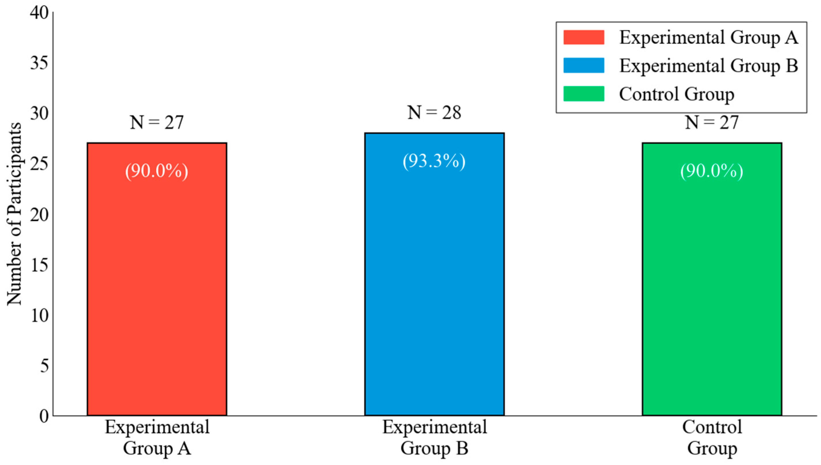
The initial enrollment for this experiment was 90 participants, with 30 participants in each group. During the experiment, some participants withdrew due to academic conflicts, illness or injury, or personal reasons. The final valid sample sizes were as follows: Experimental Group A, 27 participants (response rate: 90.0%); Experimental Group B, 28 participants (response rate: 93.3%); and the Control Group, 27 participants (response rate: 90.0%). The response rates for all three groups exceeded 80%, meeting the quality control requirements of the experimental design. The participant enrollment, group allocation, attrition reasons, and final sample sizes are summarized in Figure 2.

A one-way analysis of variance (ANOVA) was conducted to compare the baseline characteristics of the three groups of participants. The results showed no significant differences among the three groups in age $F(2, 79)=1.14,p=0.324$, height $F(2, 79)=0.95,p=0.392$, weight $F(2, 79)=0.68,p=0.510$, BMI $F(2, 79)=1.10,p=0.337$, pre-test SQM score $F(2, 79)=0.40,p=0.673$, or pre-test MAC score $F(2, 79)=0.64,p=0.530$. Gender distribution also did not differ significantly among the three groups ${\chi }^2\left(2\right)=1.21,p=0.546$. These results indicate that the baseline characteristics of the three groups were balanced and comparable before the intervention. The specific results are shown in

Table 10. Comparison of Baseline Characteristics.

Measure	Experimental Group A (n = 27)	Experimental Group B (n = 28)	Control Group (n = 27)	p-Value
Valid sample size, n	27	28	27	—
Male, n (%)	15 (55.6%)	14 (50.0%)	11 (40.7%)	0.546
Female, n (%)	12 (44.4%)	14 (50.0%)	16 (59.3%)	0.546
Age (years)	19.6 ± 1.1	20.1 ± 1.0	19.7 ± 1.4	0.324
Height (cm)	171.0 ± 6.3	173.5 ± 6.6	171.0 ± 10.0	0.392
Weight (kg)	64.8 ± 9.4	63.6 ± 15.3	67.3 ± 10.0	0.510
BMI (kg/m2)	22.3 ± 3.6	21.3 ± 5.9	23.2 ± 4.0	0.337
Pre-test SQM score	42.6 ± 3.1	42.2 ± 3.3	42.9 ± 2.2	0.673
Pre-test MAC score	3.1 ± 0.7	3.0 ± 0.6	3.2 ± 0.7	0.530

.

3.2. Analysis of SQM Scores

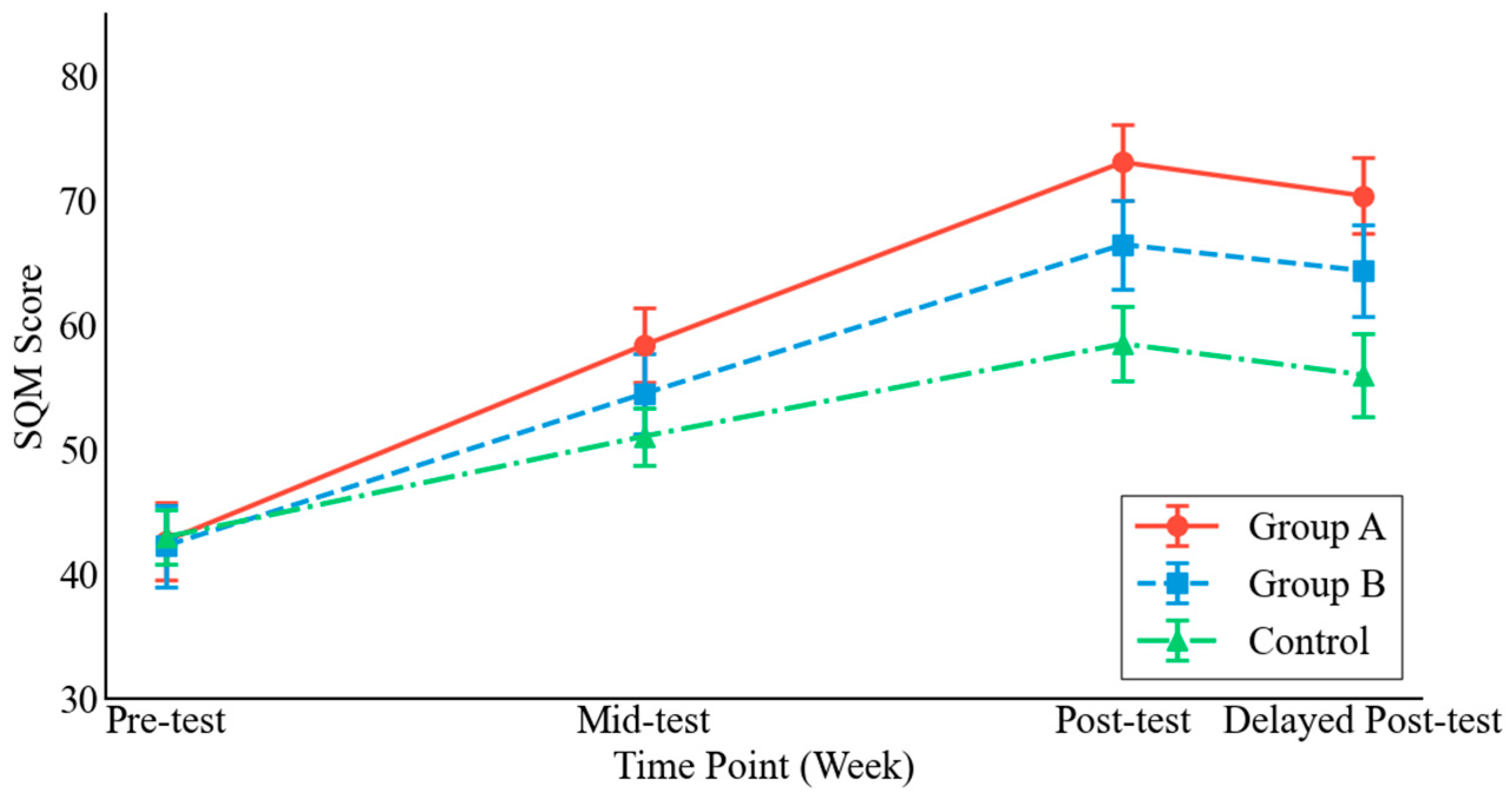
The changes in SQM scores across the four time points for each group are shown in Figure 3. Scores for all three groups showed a gradual upward trend. Experimental Group A scored higher than the other two groups at every time point, and the gap between groups gradually widened as training progressed. The specific results are shown in Figure 3.

A paired-sample t-test was used to analyze changes in SQM scores within each group before and after training. The results showed that SQM scores increased significantly in all three groups after the 8-week intervention $p<0.001$. Experimental Group A showed the largest increase in SQM score, +30.5 points, $\mathrm{t}=35.31,p<0.001,\mathrm{C}\mathrm{o}\mathrm{h}\mathrm{e}\mathrm{n}\mathrm{’}\mathrm{s} \mathrm{d}=6.80$, followed by Experimental Group B +24.2 points,$\mathrm{t}=26.90,p<0.001,\mathrm{C}\mathrm{o}\mathrm{h}\mathrm{e}\mathrm{n}\mathrm{’}\mathrm{s} \mathrm{d}=5.08$ and the Control Group +15.5 points, $\mathrm{t}=18.89,p<0.001,\mathrm{C}\mathrm{o}\mathrm{h}\mathrm{e}\mathrm{n}\mathrm{’}\mathrm{s} \mathrm{d}=3.64$. The specific results are shown in

Table 11. Pre–Post Changes in SQM Scores Across the Three Training Groups.

Group	Pre-Test	Post-Test	Change	t-Value	p-Value	Cohen’s d
Experimental Group A (n = 27)	42.6 ± 3.1	73.1 ± 3.0	+30.5	35.31	<0.001	6.80
Experimental Group B (n = 28)	42.2 ± 3.3	66.5 ± 3.6	+24.2	26.90	<0.001	5.08
Control Group (n = 27)	42.9 ± 2.2	58.5 ± 3.0	+15.5	18.89	<0.001	3.64

.

Table 11 summarizes within-group changes in human serve-training outcomes from pre-test to post-test. These changes should be interpreted as training-performance improvements observed under different instructional conditions rather than as direct measurements of algorithmic accuracy or isolated algorithmic effectiveness.

The results of the one-way ANOVA indicated significant differences in post-test SQM scores among the three groups $\mathrm{F}\left(2,79\right)=139.58,p<0.001$. The omnibus effect size was large ${\eta }^2=0.78$, 95%, $\mathrm{C}\mathrm{I}=\left[\mathrm{0.69,0.83}\right]$ and the achieved statistical power for the overall group comparison was greater than 0.99 at $\alpha =0.05$. Bonferroni-corrected pairwise comparisons showed that Experimental Group A scored significantly higher than the Control Group $\mathrm{m}\mathrm{e}\mathrm{a}\mathrm{n} \mathrm{d}\mathrm{i}\mathrm{f}\mathrm{f}\mathrm{e}\mathrm{r}\mathrm{e}\mathrm{n}\mathrm{c}\mathrm{e}=14.6 \mathrm{p}\mathrm{o}\mathrm{i}\mathrm{n}\mathrm{t}\mathrm{s}, p<0.001,\mathrm{C}\mathrm{o}\mathrm{h}\mathrm{e}\mathrm{n}\mathrm{’}\mathrm{s} \mathrm{d}=4.86$ and Experimental Group B $\mathrm{m}\mathrm{e}\mathrm{a}\mathrm{n} \mathrm{d}\mathrm{i}\mathrm{f}\mathrm{f}\mathrm{e}\mathrm{r}\mathrm{e}\mathrm{n}\mathrm{c}\mathrm{e}=6.6 \mathrm{p}\mathrm{o}\mathrm{i}\mathrm{n}\mathrm{t}\mathrm{s}, p<0.001,\mathrm{C}\mathrm{o}\mathrm{h}\mathrm{e}\mathrm{n}\mathrm{’}\mathrm{s} \mathrm{d}=1.99$. Experimental Group B also scored significantly higher than the Control Group $\mathrm{m}\mathrm{e}\mathrm{a}\mathrm{n} \mathrm{d}\mathrm{i}\mathrm{f}\mathrm{f}\mathrm{e}\mathrm{r}\mathrm{e}\mathrm{n}\mathrm{c}\mathrm{e}=8.0 \mathrm{p}\mathrm{o}\mathrm{i}\mathrm{n}\mathrm{t}\mathrm{s}, p<0.001,\mathrm{C}\mathrm{o}\mathrm{h}\mathrm{e}\mathrm{n}\mathrm{’}\mathrm{s} \mathrm{d}=2.41$. The specific results are shown in

Table 12. Between-Group Comparisons of Post-Test SQM Scores.

Comparison Group	Mean Difference	Standard Error	95% CI	p-Value	Cohen’s d
Group A vs. Control Group	+14.6	0.88	[12.9, 16.3]	<0.001	4.86
Group B vs. Control Group	+8.0	0.87	[6.3, 9.7]	<0.001	2.41
Group A vs. Group B	+6.6	0.87	[4.9, 8.3]	<0.001	1.99

Note: The omnibus one-way ANOVA showed a significant group effect on post-test SQM scores $\mathrm{F}(2,79)=139.58,p<0.001$, ${\eta }^2=0.78$, $95\%$, $\mathrm{C}\mathrm{I}=\left[\mathrm{0.69,0.83}\right]$. The achieved statistical power for the overall group comparison was greater than 0.99 at $\alpha =0.05$. Pairwise comparisons were performed using the Bonferroni correction. CI = confidence interval; SQM = Serve Quality Mastery.

.

3.3. Analysis of Movement Assessment Criteria (MAC) Scores

The MAC scores for the three groups of participants were evaluated by three professional tennis coaches, and the results are shown in

Table 13. Movement Assessment Criteria (MAC) Score Results.

Test Time Point	Group A (n = 27)	Group B (n = 28)	Control Group (n = 27)
Pre-test	3.1 ± 0.7	3.0 ± 0.6	3.2 ± 0.7
Post-test	7.9 ± 0.9	6.8 ± 0.9	5.9 ± 0.9
Change	+4.8	+3.7	+2.7

Note: Values are presented as mean ± standard deviation. MAC = Movement Assessment Criteria. The change value was calculated as post-test score minus pre-test score. Inter-rater reliability was assessed using a two-way mixed-effects, absolute-agreement, average-measures intraclass correlation coefficient ([ICC(3,k)]).

. The post-test MAC scores were higher than the pre-test scores in all three groups. Experimental Group A showed the highest post-test MAC score $7.9\pm 0.9$, followed by Experimental Group B $6.8\pm 0.9$ and the Control Group $5.9\pm 0.9$.

The inter-rater reliability analysis showed good reliability among the three professional coaches using a two-way mixed-effects, absolute-agreement, average-measures intraclass correlation coefficient $\left[ICC\right(3,k\left)\right]$, with $ICC=0.87$ (95%, $\mathit{CI}:0.82–0.91$). The Kruskal–Wallis test showed significant between-group differences in post-test MAC scores $H\left(2\right)=36.19,p<0.001$.

3.4. Analysis of Training Efficiency

There were significant differences among the three groups in the time taken to reach the SQM passing score (≥60 points) and the MAC good performance score (≥6 points), with an overall pattern of “Experimental Group A < Experimental Group B < Control Group.” as shown in

Table 14. Time Required to Reach Predefined SQM and MAC Thresholds.

Criteria	Group A	Group B	Control Group	F-Value	p-Value	${\mathsf{\eta }}^2$
SQM ≥ 60	4.1 ± 0.5	5.8 ± 0.7	7.1 ± 0.8	127.89	<0.001	0.76
MAC ≥ 6	4.6 ± 0.4	6.3 ± 0.7	7.6 ± 0.6	175.22	<0.001	0.82

Note: Values are presented as mean ± standard deviation and indicate the number of weeks required to reach the predefined thresholds. SQM = Serve Quality Mastery; MAC = Movement Assessment Criteria. Between-group differences were analyzed using one-way ANOVA ${\eta }^2=\mathrm{e}\mathrm{t}\mathrm{a} \mathrm{s}\mathrm{q}\mathrm{u}\mathrm{a}\mathrm{r}\mathrm{e}\mathrm{d}$.

.

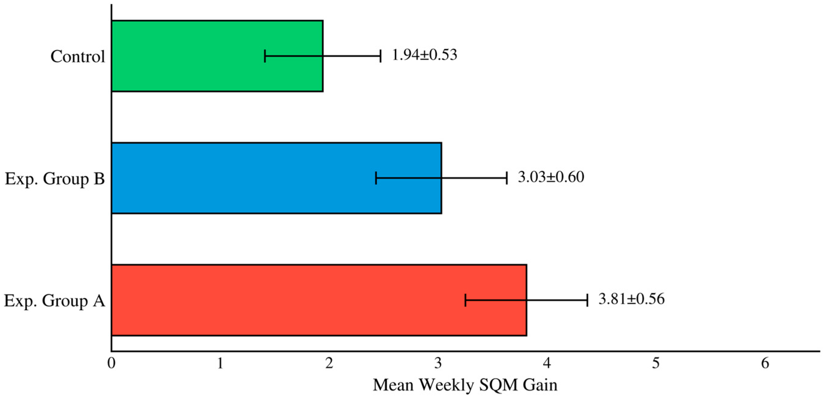
The results of the mean weekly SQM gain analysis are shown in Figure 4. Experimental Group A had the highest mean weekly SQM gain $3.81\pm 0.56$, followed by Experimental Group B $3.03\pm 0.60$ and the Control Group $1.94\pm 0.53$. The mean weekly SQM gain of Experimental Group A was 1.96 times that of the Control Group. A one-way ANOVA showed significant between-group differences in mean weekly SQM gain $F\left(2, 79\right)=74.30,p<0.001, {\eta }^2=0.65$.

In addition to the time required to reach the predefined SQM and MAC thresholds, a descriptive mean weekly SQM gain was calculated to summarize the average rate of SQM improvement during the 8-week intervention:

$$G_{\mathrm{S}\mathrm{Q}\mathrm{M}}={\displaystyle \frac{SQ{M}_{\mathrm{p}\mathrm{o}\mathrm{s}\mathrm{t}}-SQ{M}_{\mathrm{p}\mathrm{r}\mathrm{e}}}{T}}$$

(23)

where $\mathrm{S}\mathrm{Q}{\mathrm{M}}_{\mathrm{p}\mathrm{o}\mathrm{s}\mathrm{t}}$ and $\mathrm{S}\mathrm{Q}{\mathrm{M}}_{\mathrm{p}\mathrm{r}\mathrm{e}}$ represent the post-test and pre-test Serve Quality Mastery scores, respectively, and $\mathrm{T}$ represents the duration of the intervention in weeks. In this study $\mathrm{T}=8$. This value was used only as a descriptive training efficiency indicator and should not be interpreted as a validated or universally recognized measurement scale.

4. Discussion

This study evaluated a monocular pose-based, rule-driven feedback system for beginner tennis serve instruction. The results demonstrate a clear graded pattern across the three intervention conditions: greater frequency of system-generated feedback was consistently associated with larger improvements in serve performance over the 8-week intervention. This pattern suggests that timely, quantitative, and repeated corrective prompts may support early-stage motor learning by helping beginner players identify and adjust specific technical deviations that are difficult to perceive through unaided self-monitoring. The multidimensional feedback framework covering toss-arm elevation, arm extension, trunk inclination, and follow-through duration provided structured instructional cues tied to serve-specific biomechanical thresholds, which may have reinforced phase-by-phase technical refinement across repeated practice sessions. The results indicate that after 8 weeks of training, the SQM scores of all three groups of participants improved significantly, especially those of Experimental Group A. This was followed by Experimental Group B, which improved by 24.2 points, and the Control Group, which improved by 15.5 points. The between-group difference in SQM improvement was large ${\eta }^2=0.65$, indicating a clear graded pattern across the three intervention conditions.

The greater improvements observed in the feedback groups may be associated with the provision of timely and quantitative movement feedback, which could help learners identify and correct technical deviations during training. The system provides structured quantitative indicators derived from pose landmarks and rule-based thresholds, which may supplement coach observation but do not replace expert evaluation or independently validate algorithmic performance. The rule-based corrective feedback provides targeted instructional prompts according to predefined biomechanical thresholds and serve-phase rules. The multidimensional feedback framework covers four observable components—toss-arm elevation, arm extension, trunk inclination, and follow-through duration—providing structured feedback on selected aspects of the tennis serve.

A graded pattern was observed across the three groups: the high-frequency feedback group, which received system-generated feedback four times per week, demonstrated greater improvement than the moderate-frequency feedback group, which received feedback twice per week; the moderate-frequency feedback group, in turn, demonstrated greater improvement than the conventional training group. Experimental Group A reached the predefined SQM passing threshold in $4.1\pm 0.5$ weeks, approximately 42% faster than the Control Group, which required $7.1\pm 0.8$ weeks. Inter-rater reliability among the three professional coaches for the MAC scores was good (ICC (3, k) = 0.87, 95% CI: 0.82–0.91), indicating that the coaches applied the movement assessment criteria consistently with one another. It is important to note that MAC and SQM are entirely separate outcome measures: MAC scores were assigned independently by coaches without reference to any system output, while SQM scores were computed automatically by the rule-based system from pose-derived kinematic indicators. The ICC result therefore reflects coach-to-coach consistency in MAC ratings only and should not be interpreted as agreement between the system and expert evaluation, nor as evidence of the concurrent validity of the system’s scoring thresholds or rule parameters.

It should also be emphasized that the observed improvements cannot be attributed to a single technical component of the system. The intervention combined monocular pose estimation, an approximate 3D pose representation, rule-based corrective feedback, and repeated exposure to structured feedback. Therefore, the present quasi-experimental design does not allow the separate effects of the approximate 3D pose representation, the feedback rules, learner engagement, coach attention, or feedback frequency to be isolated. The findings should be interpreted as evidence of training outcomes associated with the complete feedback-supported training condition rather than as proof that any single algorithmic component independently caused the observed improvements.

These findings can be further contextualized in relation to recent work on monocular 3D human pose estimation in sports. VideoPose3D and related temporal pose-lifting methods mainly aim to estimate three-dimensional pose sequences from two-dimensional keypoint trajectories and are commonly evaluated using algorithmic accuracy metrics such as MPJPE, P-MPJPE, and PCK. Recent sports-oriented pose-estimation studies also indicate that athletic movements introduce additional challenges because they involve rapid, high-acceleration, and sport-specific motion patterns. In contrast, the present study does not attempt to outperform VideoPose3D-type methods in 3D pose-estimation accuracy. Its contribution lies in integrating an accessible pose-estimation framework, an approximate 3D pose representation, rule-based movement assessment, and corrective feedback into a practical training-support workflow for beginner tennis serve instruction.

This study has certain limitations. The sample consisted solely of college students aged 18–22 with no prior tennis experience, limiting its generalizability; while the 8-week experimental period was sufficient to evaluate short-term training outcomes, the long-term retention of skills requires further tracking; system performance is influenced by video recording quality; and the quasi-experimental design lacks true randomization. In addition, the study did not collect synchronized marker-based motion-capture data or calibrated multi-camera ground-truth data. Therefore, the metric accuracy of the approximate 3D pose representation could not be evaluated using MPJPE, P-MPJPE, PCK, or 3D joint-position error. The present findings should be interpreted as evidence concerning training outcomes and practical feasibility rather than validation of absolute 3D reconstruction accuracy. Future research could explore longitudinal tracking, expansion to diverse populations, and validation against reference motion-capture or calibrated multi-camera systems. This study provides theoretical and empirical support for integrating pose-based feedback technology into tennis teaching and training practices, offering broad prospects for application.

5. Conclusions

This study developed a monocular pose-based tennis serve analysis system and evaluated its use as a rule-driven feedback tool for beginner tennis instruction. The system integrates MediaPipe-based landmark extraction, joint-angle calculation, serve-phase recognition, an approximate 3D pose representation, and rule-based corrective feedback into a practical training-support workflow.

The quasi-experimental results show that the feedback-supported training condition was associated with greater improvements in beginner tennis serve performance than conventional instruction alone. A clear graded pattern was observed across the intervention conditions, with the high-frequency feedback group showing the greatest improvement, followed by the moderate-frequency feedback group and the conventional training group. These findings support the pedagogical usefulness of structured and repeated pose-based feedback as a supplementary instructional tool during early-stage serve learning.

The main scientific contribution of this study is the integration of accessible monocular pose estimation, biomechanically interpretable movement indicators, approximate 3D pose representation, and transparent rule-based feedback for sports training applications. The study demonstrates the practical feasibility of applying pose-derived movement information to beginner tennis serve instruction, while distinguishing this contribution from the development of a new 3D pose-estimation backbone or the validation of metric-level 3D reconstruction accuracy.

However, the present findings should be interpreted as evidence of training outcomes associated with the complete feedback-supported instructional workflow, rather than as independent quantitative validation of the computational system itself. The study did not include algorithmic validation against marker-based motion capture or calibrated multi-camera ground-truth data. Therefore, the results cannot establish the metric accuracy of the approximate 3D pose representation or independently validate the pose-estimation, phase-recognition, scoring, and feedback-generation components. In addition, the quasi-experimental design does not allow the separate effects of rule-based feedback, learner engagement, system use, feedback frequency, coach attention, and the approximate 3D component to be isolated.

Future studies should include larger and more diverse participant samples, longer follow-up periods, and independent algorithmic validation against synchronized marker-based motion capture or calibrated multi-camera reference data. Further work should also evaluate the metric accuracy of the approximate 3D pose representation using indicators such as MPJPE, P-MPJPE, PCK, 3D joint-position error, and joint-angle error, and compare the proposed workflow with temporal pose-lifting methods such as VideoPose3D. Future experimental designs should also include component-level ablation or factorial comparisons to distinguish the effects of feedback frequency, rule-based feedback, learner engagement, coach attention, and the approximate 3D representation. Accordingly, the present results should not be interpreted as demonstrating the superiority of the approximate 3D estimation method; rather, they support the practical usefulness of the complete rule-based feedback system for beginner tennis serve instruction.

References

- Amor-Salamanca, M.S.; Rodríguez-González, E.M.; Rosselló, D.; de Lluc-Bauza, M.; Hermosilla-Perona, F.; Martín-Castellanos, A.; Herrera-Peco, I. Risk Factors and Prevention of Musculoskeletal Injuries in Adolescent and Adult High-Performance Tennis Players: A Systematic Review. Sports 2025, 13, 336. [Google Scholar] [CrossRef] [Scilit]
- Kovacs, M.S. Applied physiology of tennis performance. Br. J. Sports Med. 2006, 40, 381–386. [Google Scholar] [CrossRef] [Scilit] [PubMed]
- Teferi, G.; Endalew, D. Methods of Biomechanical Performance Analyses in Sport: Systematic Review. Am. J. Sports Sci. Med. 2020, 8, 47–52. [Google Scholar] [CrossRef]
- Samkari, E.; Arif, M.; Alghamdi, M.; Al Ghamdi, M.A. Human Pose Estimation Using Deep Learning: A Systematic Literature Review. Mach. Learn. Knowl. Extr. 2023, 5, 1612–1659. [Google Scholar] [CrossRef] [Scilit]
- Lan, G.; Wu, Y.; Hu, F.; Hao, Q. Vision-Based Human Pose Estimation via Deep Learning: A Survey. IEEE Trans. Hum.-Mach. Syst. 2023, 53, 253–268. [Google Scholar] [CrossRef] [Scilit]
- Wang, J.; Tan, S.; Zhen, X.; Xu, S.; Zheng, F.; He, Z.; Shao, L. Deep 3D Human Pose Estimation: A Review. Comput. Vis. Image Underst. 2021, 210, 103225. [Google Scholar] [CrossRef] [Scilit]
- Zhang, Z.; Shin, S.-Y. Two-Dimensional Human Pose Estimation with Deep Learning: A Review. Appl. Sci. 2025, 15, 7344. [Google Scholar] [CrossRef] [Scilit]
- Huang, R.; Zhang, B.; Yao, Z.; Xie, B.; Guo, J. DESNet: Real-Time Human Pose Estimation for Sports Applications Combining IoT and Deep Learning. Alex. Eng. J. 2025, 112, 293–306. [Google Scholar] [CrossRef] [Scilit]
- Fischler, M.A.; Elschlager, R.A. The Representation and Matching of Pictorial Structures. IEEE Trans. Comput. 1973, C-22, 67–92. [Google Scholar] [CrossRef] [Scilit]
- Felzenszwalb, P.; McAllester, D.; Ramanan, D. A Discriminatively Trained, Multiscale, Deformable Part Model. In Proceedings of the 2008 IEEE Conference on Computer Vision and Pattern Recognition, Anchorage, AK, USA, 23–28 June 2008; pp. 1–8. [Google Scholar] [CrossRef] [Scilit]
- Toshev, A.; Szegedy, C. DeepPose: Human Pose Estimation via Deep Neural Networks. In Proceedings of the 2014 IEEE Conference on Computer Vision and Pattern Recognition (CVPR), Columbus, OH, USA, 23–28 June 2014; pp. 1653–1660. [Google Scholar] [CrossRef] [Scilit]
- Wei, S.-E.; Ramakrishna, V.; Kanade, T.; Sheikh, Y. Convolutional Pose Machines. In Proceedings of the 2016 IEEE Conference on Computer Vision and Pattern Recognition (CVPR), Las Vegas, NV, USA, 27–30 June 2016; pp. 4724–4732. [Google Scholar] [CrossRef] [Scilit]
- Newell, A.; Yang, K.; Deng, J. Stacked Hourglass Networks for Human Pose Estimation. Lect. Notes Comput. Sci. 2016, 9912, 29. [Google Scholar] [CrossRef] [Scilit]
- Cao, Z.; Hidalgo, G.; Simon, T.; Wei, S.-E.; Sheikh, Y. OpenPose: Realtime Multi-Person 2D Pose Estimation Using Part Affinity Fields. IEEE Trans. Pattern Anal. Mach. Intell. 2021, 43, 172–186. [Google Scholar] [CrossRef] [Scilit] [PubMed]
- Sun, K.; Xiao, B.; Liu, D.; Wang, J. Deep High-Resolution Representation Learning for Human Pose Estimation. In Proceedings of the 2019 IEEE/CVF Conference on Computer Vision and Pattern Recognition (CVPR), Long Beach, CA, USA, 15–20 June 2019; pp. 5686–5696. [Google Scholar] [CrossRef] [Scilit]
- El Kaid, A.; Baïna, K. A Systematic Review of Recent Deep Learning Approaches for 3D Human Pose Estimation. J. Imaging 2023, 9, 275. [Google Scholar] [CrossRef] [Scilit] [PubMed]
- Zhou, X.; Zhu, M.; Leonardos, S.; Derpanis, K.G. Sparseness Meets Deepness: 3D Human Pose Estimation from Monocular Video. In Proceedings of the 2016 IEEE Conference on Computer Vision and Pattern Recognition (CVPR), Las Vegas, NV, USA, 27–30 June 2016; pp. 4966–4975. [Google Scholar] [CrossRef] [Scilit]
- Zheng, C.; Wu, W.; Chen, C.; Yang, T.; Zhu, S.; Shen, J.; Kehtarnavaz, N.; Shah, M. Deep Learning-Based Human Pose Estimation: A Survey. ACM Comput. Surv. 2023, 56, 11. [Google Scholar] [CrossRef] [Scilit]
- Chen, Y.; Tian, Y.; He, M. Monocular Human Pose Estimation: A Survey of Deep Learning-Based Methods. Comput. Vis. Image Underst. 2020, 192, 102897. [Google Scholar] [CrossRef] [Scilit]
- Guo, Y.; Zhao, L.; Zhang, S.; Yang, J. Coarse-to-Fine 3D Human Pose Estimation. Lect. Notes Comput. Sci. 2019, 11903, 579–592. [Google Scholar] [CrossRef] [Scilit]
- Pavlakos, G.; Zhou, X.; Derpanis, K.G.; Daniilidis, K. Coarse-to-Fine Volumetric Prediction for Single-Image 3D Human Pose. In Proceedings of the 2017 IEEE Conference on Computer Vision and Pattern Recognition (CVPR), Honolulu, HI, USA, 21–26 July 2017; pp. 1263–1272. [Google Scholar] [CrossRef] [Scilit]
- Asriani, F.; Azhari, A.; Wahyono, W. Improving Badminton Action Recognition Using Spatio-Temporal Analysis and a Weighted Ensemble Learning Model. Comput. Mater. Contin. 2024, 81, 3079–3096. [Google Scholar] [CrossRef] [Scilit]
- Mitul, T.M.; Rahman, M.; Deb, K. A Deep Learning Based Approach for the Categorization of Actions in Cricket Videos. In Proceedings of the 2024 2nd International Conference on Information and Communication Technology, Dhaka, Bangladesh, 21–22 October 2024; pp. 71–75. [Google Scholar] [CrossRef] [Scilit]
- Dang, Q.; Yin, J.; Wang, B.; Zheng, W. Deep Learning Based 2D Human Pose Estimation: A Survey. Tsinghua Sci. Technol. 2019, 24, 663–676. [Google Scholar] [CrossRef] [Scilit]
- Murakami, T.; Nakamura, T. Athlete 3D Pose Estimation from a Monocular TV Sports Video Using Pre-Trained Temporal Convolutional Networks. In Proceedings of the 2020 IEEE International Conference on Systems, Man, and Cybernetics, Toronto, ON, Canada, 11–14 October 2020; pp. 2615–2620. [Google Scholar] [CrossRef] [Scilit]
- Liu, J. Automated Tennis Swing Analysis Using Pose Estimation and Optical Flow. Available online: https://web.stanford.edu/class/ee367/Winter2025/report/report_Jeffrey_Liu.pdf (accessed on 29 May 2026).
- Dong, L.; Yang, Y.; Wu, H.; Wang, W.; Hou, Y.; Zhong, Z.; Sun, X. RacketVision: A Multiple Racket Sports Benchmark for Unified Ball and Racket Analysis. Proc. AAAI Conf. Artif. Intell. 2026, 40, 3632–3640. [Google Scholar] [CrossRef] [Scilit]
- Quiñonez, Y.; Lizarraga, C.; Aguayo, R. Machine Learning Solutions with MediaPipe. In Proceedings of the 2022 11th International Conference On Software Process Improvement, Acapulco, Mexico, 19–21 October 2022; pp. 212–215. [Google Scholar] [CrossRef] [Scilit]
- Pavllo, D.; Feichtenhofer, C.; Grangier, D. 3D Human Pose Estimation in Video With Temporal Convolutions and Semi-Supervised Training. In Proceedings of the IEEE/CVF Conference on Computer Vision and Pattern Recognition (CVPR), Long Beach, CA, USA, 15–20 June 2019; pp. 7745–7754. [Google Scholar] [CrossRef] [Scilit]
- Zheng, C.; Zhu, S.; Mendieta, M.; Yang, T.; Chen, C.; Ding, Z. 3D Human Pose Estimation with Spatial and Temporal Transformers. In Proceedings of the IEEE/CVF International Conference on Computer Vision (ICCV), Virtual, 11–17 October 2021; pp. 11636–11645. [Google Scholar]
- Li, W.; Liu, H.; Tang, H.; Wang, P.; Van Gool, L. MHFormer: Multi-Hypothesis Transformer for 3D Human Pose Estimation. In Proceedings of the IEEE/CVF Conference on Computer Vision and Pattern Recognition (CVPR), New Orleans, LA, USA, 18–24 June 2022; pp. 13137–13146. [Google Scholar]
- Zhang, J.; Tu, Z.; Yang, J.; Chen, Y.; Yuan, J. MixSTE: Seq2seq Mixed Spatio-Temporal Encoder for 3D Human Pose Estimation in Video. In Proceedings of the IEEE/CVF Conference on Computer Vision and Pattern Recognition (CVPR), New Orleans, LA, USA, 18–24 June 2022; pp. 13222–13232. [Google Scholar]
- Zhu, W.; Ma, X.; Liu, Z.; Liu, L.; Wu, W.; Wang, Y. MotionBERT: A Unified Perspective on Learning Human Motion Representations. In Proceedings of the IEEE/CVF International Conference on Computer Vision (ICCV), Paris, France, 2–6 October 2023; pp. 15085–15099. [Google Scholar]
- Zhao, Q.; Zheng, C.; Liu, M.; Wang, P.; Chen, C. PoseFormerV2: Exploring Frequency Domain for Efficient and Robust 3D Human Pose Estimation. In Proceedings of the IEEE/CVF Conference on Computer Vision and Pattern Recognition (CVPR), Vancouver, BC, Canada, 17–24 June 2023; pp. 8877–8886. [Google Scholar]
- Mehraban, S.; Adeli, V.; Taati, B. MotionAGFormer: Enhancing 3D Human Pose Estimation with a Transformer-GCNFormer Network. In Proceedings of the IEEE/CVF Winter Conference on Applications of Computer Vision (WACV), Waikoloa, HI, USA, 3–8 January 2024; pp. 6690–6700. [Google Scholar] [CrossRef] [Scilit]
- He, J.; Yang, W. Video-Based Human Pose Regression via Decoupled Space-Time Aggregation. In Proceedings of the IEEE/CVF Conference on Computer Vision and Pattern Recognition (CVPR), Seattle, WA, USA, 16–22 June 2024; pp. 1022–1031. [Google Scholar] [CrossRef] [Scilit]
- Yeung, C.; Suzuki, T.; Tanaka, R.; Yin, Z.; Fujii, K. AthletePose3D: A Benchmark Dataset for 3D Human Pose Estimation and Kinematic Validation in Athletic Movements. In Proceedings of the IEEE/CVF Conference on Computer Vision and Pattern Recognition (CVPR) Workshops, Nashville, TN, USA, 10–11 June 2025; pp. 5991–6002. [Google Scholar]
- Kim, J.-W.; Choi, J.-Y.; Ha, E.-J.; Choi, J.-H. Human Pose Estimation Using MediaPipe Pose and Optimization Method Based on a Humanoid Model. Appl. Sci. 2023, 13, 2700. [Google Scholar] [CrossRef] [Scilit]
- Dempster, W.T.; Gaughran, G.R.L. Properties of Body Segments Based on Size and Weight. Am. J. Anat. 1967, 120, 33–54. [Google Scholar] [CrossRef] [Scilit]
- de Leva, P. Adjustments to Zatsiorsky-Seluyanov’s Segment Inertia Parameters. J. Biomech. 1996, 29, 1223–1230. [Google Scholar] [CrossRef] [Scilit] [PubMed]