Article

A Multi-Strategy Harris Hawks Optimization and Its Application in Feature Selection

1
Institute of Transportation and Economic Research, China Academy of Railway Sciences Corporation Limited, Beijing 100081, China
2
School of Economics and Management, Beijing Jiaotong University, Beijing 100044, China
*
Author to whom correspondence should be addressed.
Appl. Sci. 2026, 16(13), 6488; https://doi.org/10.3390/app16136488
Submission received: 25 February 2026 / Revised: 13 April 2026 / Accepted: 15 April 2026 / Published: 29 June 2026

Abstract

Feature selection (FS) is a pivotal preprocessing task in data mining aimed at identifying optimal feature subsets to improve model generalization and reduce computational overhead. However, its NP-hard nature poses significant challenges for traditional optimizers in terms of search efficiency and solution quality. The Harris Hawks Optimization (HHO) algorithm is a state-of-the-art population-based metaheuristic method that demonstrates powerful capabilities in various optimization challenges. Despite its advantages, HHO encounters problems such as early stagnation and reduced accuracy. To mitigate these problems, we introduce an advanced algorithm called the Hybrid Strategy Harris Hawks Optimization (HSHHO). The HSHHO combines three key enhancements to support global search diversity and local refinement: (1) an exploration mechanism that utilizes the Self-Parameterized Map (SPM) alongside a dynamic logarithmic spiral to expand search breadth; (2) a nonlinear adjustment to the escape energy parameter for improved phase equilibrium; and (3) an elite perturbation approach that uses Cauchy–Gaussian mutation to strengthen local optimization and solution quality. We assessed HSHHO against eight well-known algorithms on 30 benchmark functions, where it exhibited superior results in the majority of cases. Finally, HSHHO is applied to address 18 feature selection tasks. The results demonstrated that HSHHO achieved highly competitive outcomes in terms of objective values, feature subset size, and classification performance in most datasets, reaching an average accuracy of 94.47%.

1. Introduction

Nowadays, various industries generate a large amount of data, and finding valuable insights from multi-source data is a daunting challenge for data processing [1]. Model performance often requires clean, non-redundant input data. However, the collected raw data often has redundant, irrelevant, and noisy features [2]. High-dimensional data can lead to a curse of dimensionality, severely reducing the model’s generalization ability.
To address these issues, researchers widely use feature selection (FS) methods to identify key attributes in the data. The goal of feature selection is to find the optimal subset of features to eliminate irrelevant or redundant features, thereby improving model accuracy and reducing computational complexity [3]. Essentially, FS is a combinatorial optimization problem, where given a dataset with  n  features, the objective is to select the optimal feature subset from  2 n  candidate feature combinations [4]. Due to its NP hard nature and inherent multi-objective nature, this task has attracted in-depth research in recent years [5]. At present, the FS method has been applied in classification and regression tasks [6,7], engineering optimization [8,9], text classification [10,11], and many other fields. Especially in complex engineering applications, such as railway transportation emergency response scenarios, due to the involvement of multi-disciplinary collaboration, the emergency response process generates massive amounts of multi feature data. Researchers need to identify key influencing factors from these redundant and noisy raw features. FS, as a key preprocessing task, can effectively eliminate irrelevant variables in railway emergency data, thereby improving emergency decision-making capabilities in the event of sudden accidents.
FS approaches fall into three categories: filter, wrapper, and embedded methods [12,13,14,15,16]. Filter methods are computationally lightweight and classifier-independent, which explains their widespread popularity. However, they often produce suboptimal feature subsets and are prone to overfitting [17]. Wrapper methods, by contrast, evaluate subsets directly through a specific classifier; although they are more accurate and less susceptible to overfitting than filters, they can still select biased features when used in isolation and are computationally more demanding. Embedded methods integrate feature selection into the training process of the classifier itself and have therefore drawn considerable interest; numerous hybrid strategies have been proposed to further enhance their effectiveness [18,19]. Regardless of category, these techniques are typically paired with well-known classifiers such as decision trees [20,21], support vector machines [22], Bayesian networks [23,24], k-nearest neighbors [25], and artificial neural networks [26,27].
In recent years, metaheuristic optimization algorithms have become the main method for solving FS problems due to their powerful global search and local optimization capabilities [28,29,30,31,32,33]. The landscape optimized by metaheuristics can be divided into two main schools of thought. The first genre includes mature classic algorithms that have been rigorously tested for decades, such as genetic algorithms (GA), differential evolution (DE), and simulated annealing (SA). The second school represents recent biologically inspired swarm intelligence methods that utilize collective behavior in nature to solve complex engineering problems. For example, Particle Swarm Optimization (PSO), Gray Wolf Optimizer (GWO), Whale Optimization Algorithm (WOA), etc. These optimization algorithms can generate a set of candidate solutions. Their search process consists of two basic stages, the exploration stage and the exploitation stage [34]. However, the imbalance between the two stages is the main reason why these algorithms fall into local optima when processing high-dimensional data.
To overcome these limitations, researchers are increasingly turning to hybrid algorithms that combine complementary advantages. For example, chaotic cosine firefly (CSCF) algorithm [35], PSO-GWO hybrid algorithm [36], GSA-GA fusion algorithm [37], quantum enhanced bat algorithm (CCQBA) [38], and opponent based social spider optimizer (OBSSO) [39]. These hybrid algorithms demonstrate excellent solving capabilities in feature selection problems.
Among the popular swarm intelligence algorithms, the HHO algorithm has received widespread attention due to its simple mathematical structure and effectiveness in solving various engineering problems [40]. However, HHO performs poorly in dealing with high-dimensional and complex multimodal problems. This is because HHO has limitations of premature convergence and low solution accuracy. Therefore, it is urgent to propose improvement strategies to optimize HHO in order to enhance the algorithm’s fast gaming performance. At present, several enhancement methods have been proposed to alleviate these weaknesses: neighborhood perturbation [41], sine escape energy adjustment [42], logarithmic spiral exploration [43], and tent graph plus crossover mutation strategy [44]. Based on these insights, the present work introduces a novel algorithm called Hybrid Strategy Harris Hawks Optimization (HSHHO). As an improved feature selection wrapper method, HSHHO aims to obtain the optimal feature subset while improving classification accuracy.
The core contribution lies in three targeted improvement measures aimed at strengthening the exploration, transition, and mining stages of HHO:
(1)
SPM chaotic mapping and variable logarithmic spiral strategy were proposed to enhance burst diversity and global search.
(2)
A nonlinear escape energy function has been proposed, achieving a smoother and more adaptive balance between exploration and exploitation.
(3)
The Cauchy–Gaussian elite perturbation mechanism has been proposed, which can promote local refinement and help algorithms overcome local optima.
The rest of this article is organized as follows. Section 2 reviewed the standard HHO algorithm and proposed three improvement strategies for constructing HSHHO. Section 3 reports a comprehensive experiment on 30 benchmark functions and 18 real-world feature selection datasets, comparing HSHHO with eight well-known methods. Finally, Section 4 summarizes the research findings and outlines future research directions.

2. Methods

2.1. Harris Hawks Optimization

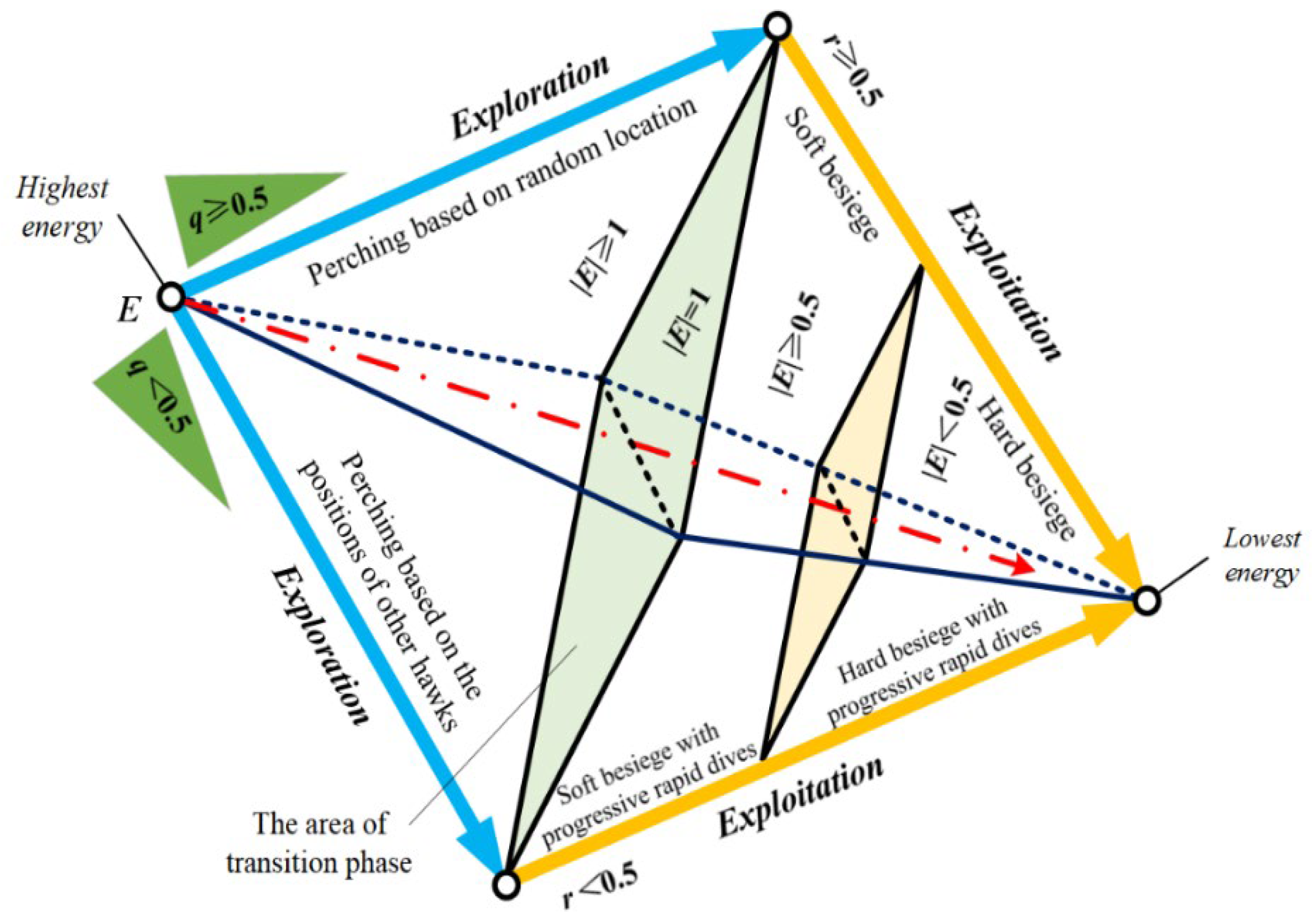
The Harris Hawks Optimization (HHO) is a population-based metaheuristic, inspired by the collaborative hunting tactics of Harris hawks in pursuing prey. This algorithm has shown robust performance in addressing various optimization challenges. To cope with the variability in prey behavior and environmental conditions, hawks adapt their strategies dynamically. Empirical evaluations indicate that HHO often surpasses other metaheuristics in terms of solution quality. The algorithm operates in two primary phases—exploration and exploitation—driven by the prey’s escape energy, as illustrated in Figure 1. Exploration employs two position-update mechanisms, while exploitation features four distinct strategies. The detail of the HHO is as follows.
Figure 1 shows the framework of the HHO algorithm, demonstrating the dynamic behavior between different hunting stages. The optimization process is mainly determined by the escape energy  E  of the prey. When  E 1 , the algorithm is in the exploration stage. When  E < 1 , the algorithm will enter the exploitation stage. In these stages, the specific strategy is determined by two variables:  q  determines the habitat mechanism during exploration, while  r  represents the probability of prey successfully escaping during exploitation. The arrow indicates the behavioral change in the eagle’s position from global search to local capture.

2.1.1. Exploration Phase

In HHO, each hawk represents a candidate solution within the population. Through iterative updates, hawks adjust their positions relative to the current best location. During exploration, two strategies are applied based on a random threshold  q . If  q     0.5 , hawks update positions using their own location and those of nearby individuals. If  q   <   0.5 , they select a random perch within the search space for observation. The mathematical formulations are:
X t + 1 = X r a n t t r 1 X r a n t t 2 r 2 X t                                                         q 0.5 X r a b b i t t X m t r 3 L B + r 4 U B L B           q < 0.5
where  X t + 1  is the expressed hawk position at iteration  t + 1 X r a n t t  is a randomly chosen hawk position at iteration  t X r a b b i t t  is the prey’s position (best solution) at iteration  t r 1 r 2 r 3 r 4  are random values in (0, 1).  U B  and  L B  denote the upper and lower bounds of the search space. The average population position  X m ( t )  is computed as:
X m t = 1 N i = 1 N X i t

2.1.2. Transition Phase

The transition from exploration to exploitation hinges on the prey’s escape energy  E , which dictates the hawks’ pursuit tactics. Initially, hawks scan broadly for prey; upon detection, they shift to targeted attacks. This phase ensures an equilibrium between global and local search, enhancing overall efficiency. The escape energy is modeled as:
E = 2 E 0 1 t T
where  E 0  represents is the initial escape energy, which is a random value with [−1, 1].  t  is the current iteration, and  T  is the maximum iterations.  E  decreases linearly from 2 to 0 over iterations, as depicted in the light green area of Figure 1.

2.1.3. Exploitation Phase

Exploitation encompasses four strategies, selected based on  E  and an escape probability  r . If  r 0.5 , the prey escapes successfully; otherwise, it fails. Figure 1 outlines the sequential application of these strategies.
  • Soft besiege strategy
When  E 0.5  and  r 0.5 , hawks gradually encircle the prey with sufficient energy remaining:
X t + 1 = X t E J X r a b b i t t X t
X t = X r a b b i t t X t
where  J  is a random number with [0, 2] denoting the strength of the rabbit’s jumps during its escape.  X r a b b i t t  denotes the best solution in iteration  t .
2.
Hard besiege strategy
When  E < 0.5  and  r 0.5 , the prey is fatigued, prompting a direct assault:
X t + 1 = X r a b b i t t E X t
3.
Soft besiege with progressive rapid dives
When  E 0.5  and  r < 0.5 , the prey evades energetically, leading to Lévy-flight-based dives:
Y = X r a b b i t t E J X r a b b i t t X t
Z = Y + S × L F D
X t + 1 = Y                                 i f   F Y < F X t Z                                 i f   F Z < F X t
where  S  is a random vector in [0, 1]. Y and Z denote the two strategies, respectively.  L F  denotes the Lévy flight function [45]:
L F x = 0.01 × μ × σ v 1 p
σ = Γ 1 + β × sin π β 2 Γ 1 + β 2 × β × 2 β 1 2
where  μ  and  v  normally distributed in (0, 1).  β  is 1.5 acquiescently.
4.
Hard besiege with progressive rapid dives
When  E < 0.5  and  r < 0.5 , a similar dive strategy is applied but with reduced energy:
Y = X r a b b i t t E J X r a b b i t t X m t
Z = Y + S × L F D
X t + 1 = Y                                 i f   F Y < F X t Z                                 i f   F Z < F X t

2.2. Hybrid Strategy Harris Hawks Optimization

While HHO excels in dynamic search, it shares common pitfalls with other swarm methods, such as limited accuracy and local optima entrapment when facing complex problems. These arise from random initialization and rigid exploration/exploitation mechanics. To remedy this, we propose HSHHO, incorporating: (1) SPM chaotic map and variable logarithmic spiral (SPM-VLS) for exploration; (2) nonlinear escape energy for transition; and (3) Cauchy–Gaussian elite perturbation for exploitation. The three proposed improvement strategies effectively address the inherent weaknesses of HHO. Although SPM-VLS expands the initial search range, the nonlinear energy method maintains a balance between the exploration stage and the mining stage during the mid-term iteration, and the dual mutation mechanism in the mining stage escapes the local optimal solution. This synergy ensures that each stage of the optimization process is particularly strengthened.

2.2.1. Population Initialization Based on a Chaotic Map

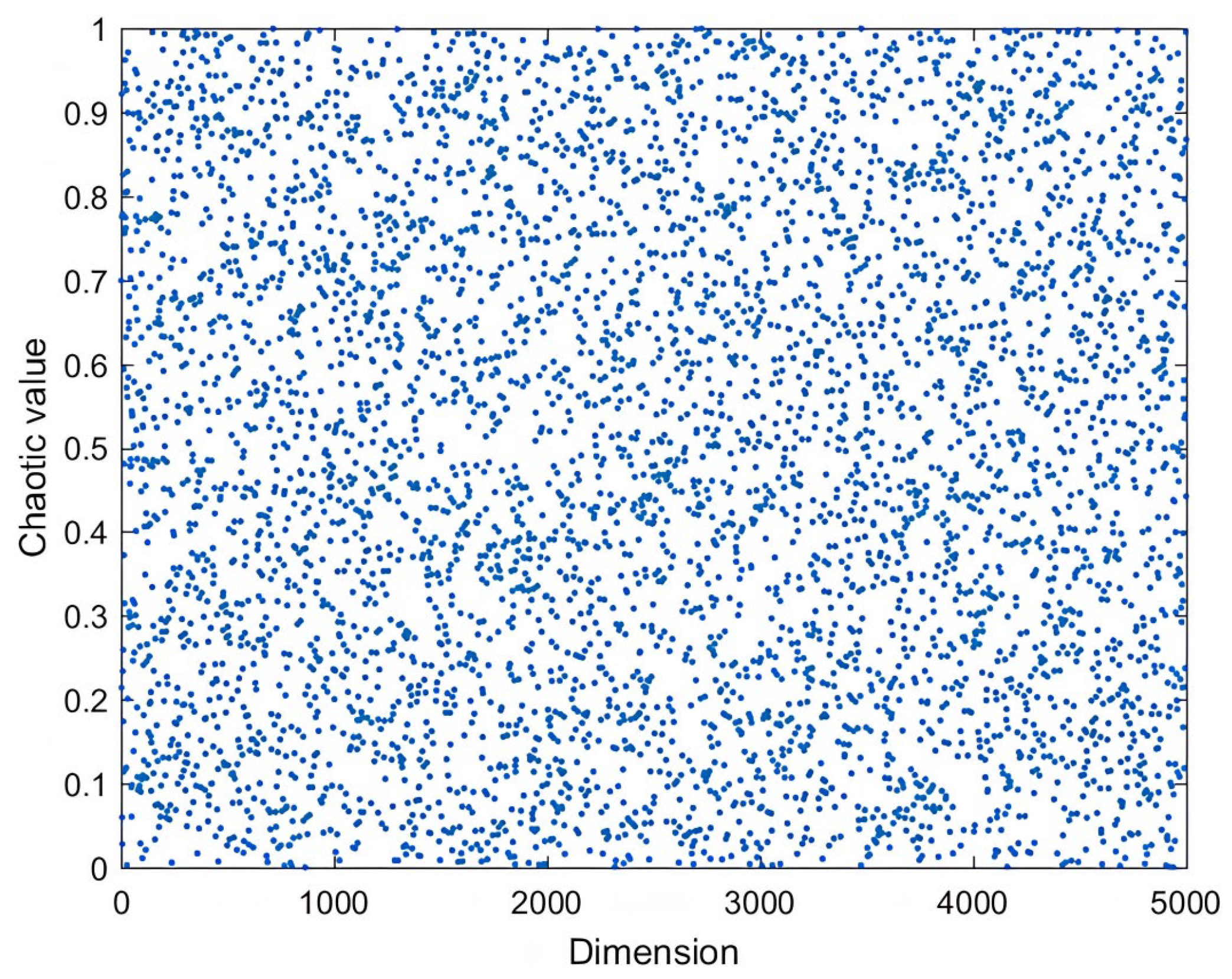
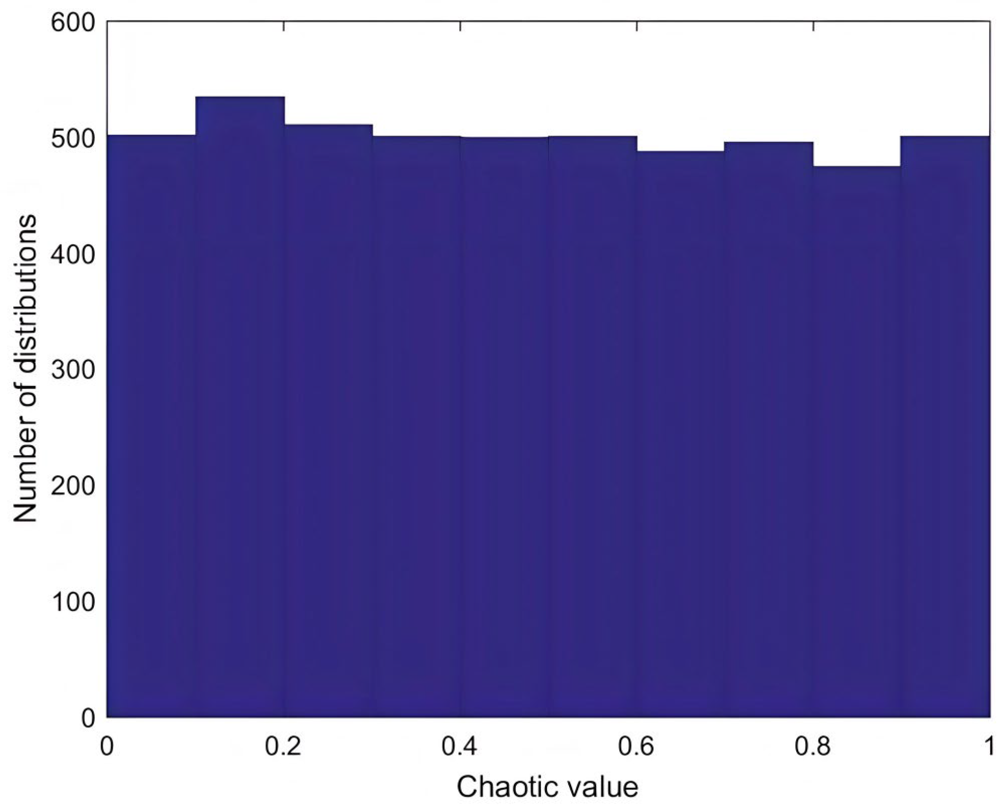
The population initialization of optimization algorithms is one of the key steps. The distribution of the population affects the search performance of the algorithm in the early stage. In the HHO algorithm, the initial population position is randomly generated, which may lead to an uneven distribution of individuals. The diversity of the initial population is the key to algorithm optimization, and it is necessary to enhance population diversity to improve overall search capability. Introducing chaotic mapping into the algorithm initialization phase can alleviate this problem. Chaotic mapping can provide traversal and non-repetitive sequences, which are superior to random initialization in improving population diversity [46]. This study chooses the SPM mapping method to replace the traditional random generation method. Figure 2 and Figure 3 show the distribution histograms and scatter plots of SPM, respectively. It is not difficult to see that the population generated using SPM mapping exhibits a uniform distribution. Therefore, SPM effectively enhances the diversity of the initial population, which is beneficial for the global search of the algorithm.
Therefore, we introduce the SPM to improve the population initialization of HHO:
x t + 1 = m o d x t μ + δ sin π x t + r , 1                     0 x t μ m o d x t μ 0.5 μ + δ sin π x t + r , 1                     μ x t 0.5 m o d 1 x t μ 0.5 μ + δ sin π 1 x t + r , 1                     0.5 x t 1 μ m o d 1 x t μ μ + δ sin π 1 x t + r , 1                     1 μ x t 1
where if  μ 0 , 1 ,   δ ( 0 , 1 ) , the system is in a chaotic state.  r ( 0 ,   1 )  is a random number.
Therefore, we can obtain the position of  x p o s i t i o n :
x p o s i t i o n = l b + x t × u b l b

2.2.2. Variable Logarithmic Spiral Strategy

HHO’s exploration relies heavily on random factors, which can lead to premature convergence. We integrate a variable logarithmic spiral, inspired by whale and moth algorithms [47], to refine position updates:
X t + 1 = X b e s t X t × e b l × c o s 2 π l + X b e s t
where  X b e s t  represents the best solution.  l  represents a random number in [−1, 1].  b  dynamically adjusts:
b = e π 1 t T
This enables larger spirals early on and finer adjustments later.

2.2.3. Improvement Strategies for the Transition Phase

The transition phase of HHO is based on the escape energy  E . The main purpose of the transition phase is to maintain a balance between exploration phase and exploitation phase. We propose a nonlinear method to address the limitation of linear function.
E t = E m i n + E m a x E m i n × c o s π 2 t T 2 q > 0.5 E m i n + E m a x E m i n × 1 X t X b e s t X m X b e s t q < 0.5
where  X m  represents the average position of the population.  E m i n  is the minimum value,  E m a x  is the maximum value.  ρ 0 , 1  of random numbers.
Equation (19) shows that  E t  varies nonlinearly with the number of iterations. Based on Figure 1, when  q > 0.5 E t  decreases nonlinearly from the exploration to the exploitation. According to the variation curve of the cos(x) function, with  E t  in the middle of the algorithm iteration, the rate of change accelerates, which enables the HHO to quickly switch to the exploitation phase. When  q < 0.5  and  E t  depends on the distance between the position of the Harris hawks and the position of the optimal solution, the closer to the optimal solution, the larger  E t  is, and the algorithm will shift from the exploitation stage to the exploration phase, which can relieve local population accumulation and avoid getting into a local optimum in the later stage of the algorithm.

2.2.4. Improvement Strategies for the Exploitation Phase

To overcome limitations of HHO, we introduce an elite-guided perturbation strategy [48]. The disturbance probability  P d i s  is introduced to determine whether the current optimal individual  X b e s t  performs the elite perturbation operation:
P d i s = D 1 × e t 1 T 4 D
where  P d i s  is the disturbance probability of an elite individual and  D  is the problem dimension.
To improve the capability of running away from local optima, an improved method is proposed by integrating the Cauchy–Gaussian mutation mechanism into the traditional elite perturbation strategy. The specific calculation formula of the Cauchy–Gaussian mutation is expressed as follows:
P o s i t o n b e s t t = X t × 1 + λ 1 C a u c h y 0 , 1 + λ 2 G u a s s 0 , 1
where  C a u c h y 0 , 1  represents a Cauchy random variable, and  G u a s s 0 , 1  represents a Gaussian variable.  λ 1 = 1 t 2 T 2 , whose value gradually decreases with the iterations,  λ 2 = t 2 T 2 , and the value gradually increases with the iterations.
Therefore, the best individual position is as shown:
X b e s t = P o s i t o n b e s t               α > P d i s F X b e s t > F X b s e t X b s e t                                                                                               o t h e r w i s e
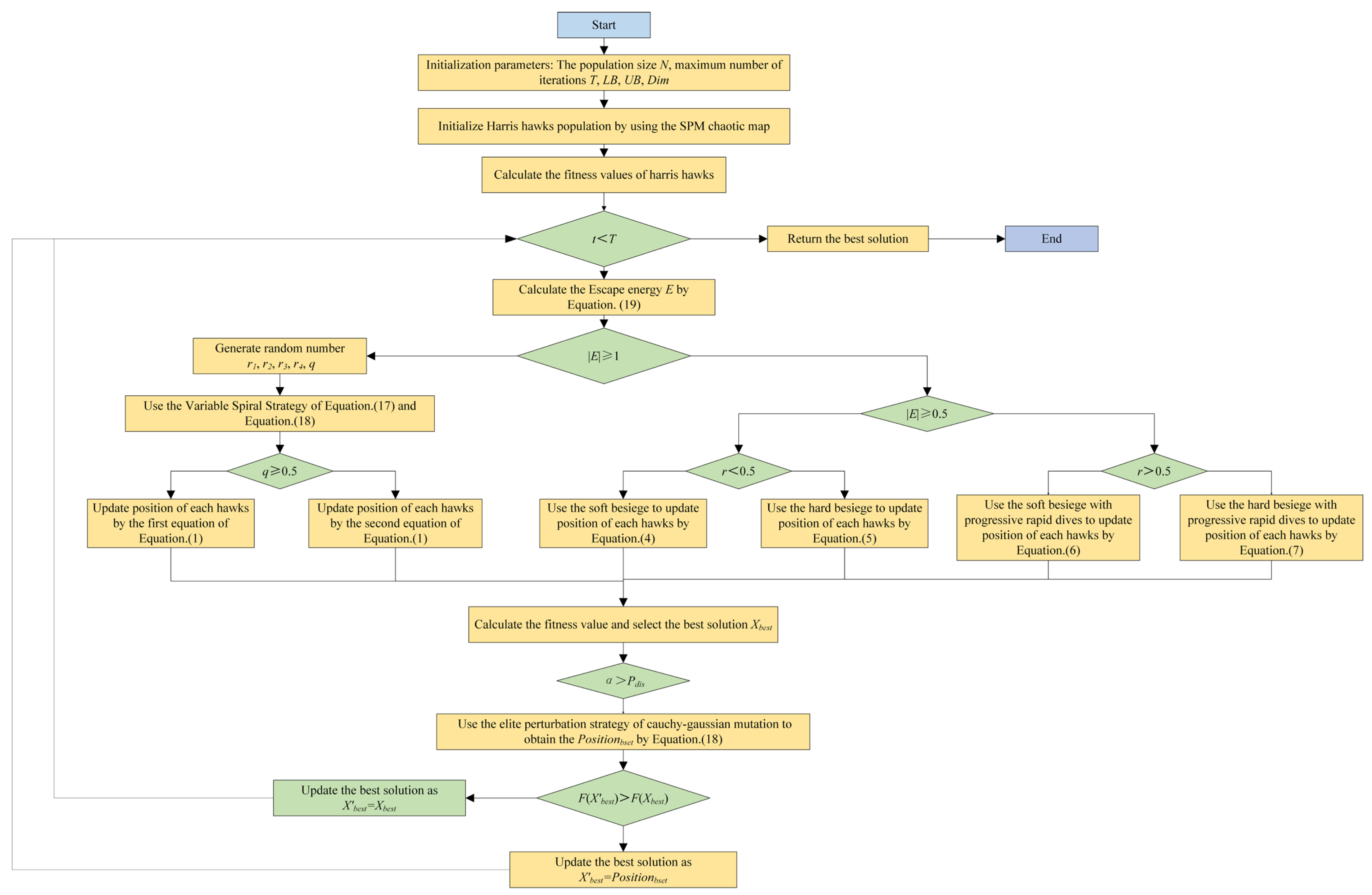
In summary, the proposed HSHHO algorithm is shown in Figure 4.

2.3. Complexity of the HSHHO Algorithm

The computational complexity of the HSHHO algorithm is mainly composed of the following three parts:
  • Initialization of the population. The computational complexity of this part mainly depends on population size  N  and the problem dimension  D , and the calculated complexity is  O ( N × D ) .
  • Evaluating the fitness of the initial population. The computational complexity of this part is mainly determined by the population size  N . The computational complexity is  O ( N ) .
  • The population position is cyclically updated. The computational complexity of this part mainly depends by the population size  N , the problem dimension  D  and the number of iterations  T . It is composed of individual position updates and fitness calculations. The position of the individual is updated through different search strategies. The execution of two different stages is determined by whether the algorithm satisfies the judgment condition. The computational complexity of this part is calculated as  O ( N × D × T ) .
Based on the above analysis, we can deduce that the time complexity of our proposed HSHHO algorithm follows a similar structure to that of the standard HHO algorithm. Specifically, the time complexity primarily includes population position initialization, population position update, and population fitness calculation. Consequently, the computational complexity of these components should remain unchanged. Similarly, the different strategy in this paper is to improve the method of updating the population position without increasing the number of populations and the iteration time, which does not change the time complexity of this component.
Therefore,  O ( H S H H O )  =  O I n i t i a l i s a t i o n   o f   t h e   H a r r i s   H a w k s   p o p u l a t i o n  +  O ( H a r r i s   H a w k s   f i t n e s s   c a l c u l a t i o n )  +  O ( H a r r i s   H a w k s   p o s i t i o n   u p d a t e ) . where  O I n i t i a l i s a t i o n   o f   t h e   H a r r i s   H a w k s   p o p u l a t i o n = O ( N × D ) O H a r r i s   H a w k s   f i t n e s s   c a l c u l a t i o n = O ( N ) O H a r r i s   H a w k s   p o s i t i o n   u p d a t e = O ( N × D × T ) . Total complexity of the HSHHO is  O H S H H O = O ( N × D × T ) .

3. Results

To assess the efficacy and optimization potential of HSHHO, we conduct a series of simulation experiments. Initially, the algorithm is tested on 23 standard benchmark functions to evaluate the impact of its three enhancement strategies relative to the baseline HHO. Subsequently, HSHHO is benchmarked against eight established metaheuristic algorithms using IEEE CEC 2017 problems, with statistical analyses to highlight its advantages. Finally, HSHHO is deployed on 18 feature selection datasets to demonstrate its practical utility. All simulations are executed on a Windows 10 system equipped with an Intel Core i7-7700, CPU @ 3.60 GHz and 32 G of RAM, using MATLAB R2022b for implementation.
The common parameters for all algorithms are set such that the population size  N  is 30 and the maximum iteration  T  is 500. In this study, to ensure fairness in computational workload between algorithms, the total number of function evaluations  F E  is set to  N × T = 15000 . In addition, we define one iteration of the algorithm as a complete loop. In this loop, the positions of all individuals in the group are updated, followed by a round of fitness assessment.

3.1. Comparison of the Effects of Different Improvement Strategies

To bolster HHO’s optimization capabilities, we introduce three targeted enhancements: a hybrid SPM chaotic map with variable logarithmic spiral (SPM-VLS), a nonlinear escape energy mechanism for smoother phase transitions, and a Cauchy–Gaussian elite perturbation approach. These are integrated to form the comprehensive HSHHO algorithm. This section aims to empirically verify the independent contribution of each strategy to HHO and demonstrate the excellent performance achieved through its fusion effect.
To conduct this analysis, we decomposed HSHHO into three variants, including HSHHO1, HSHHO2, and HSHHO3. Each variant contains only one improvement strategy. HSHHO1 only enhances HHO through SPM-VLS and ignores other functions. HSHHO2 only applies nonlinear escape energy updates. HSHHO3 is only available for the police Cauchy Gauss Elite. These variants, as well as the proposed HSHHO and HHO, are evaluated and compared on 23 standard benchmark functions, as shown in Table 1.
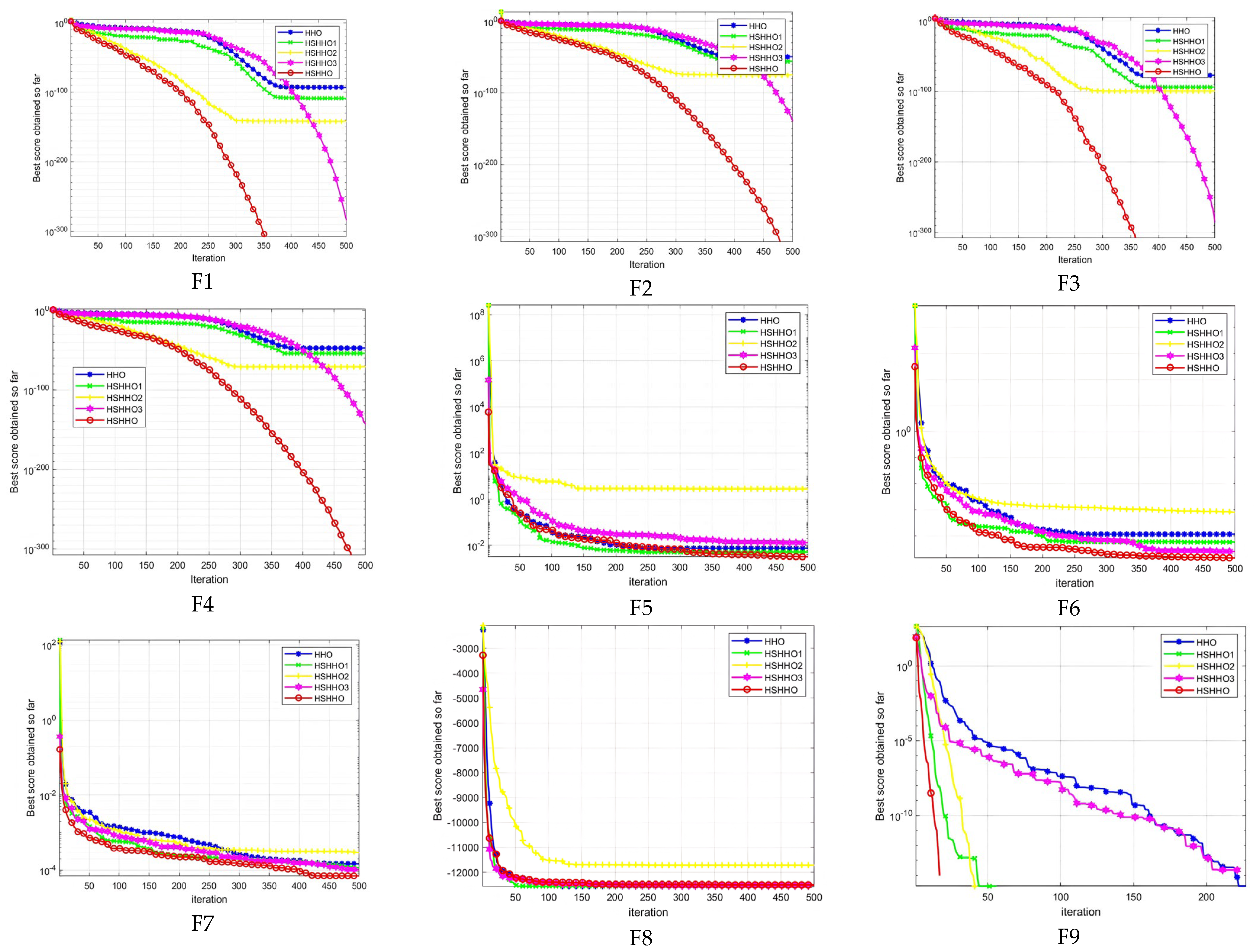
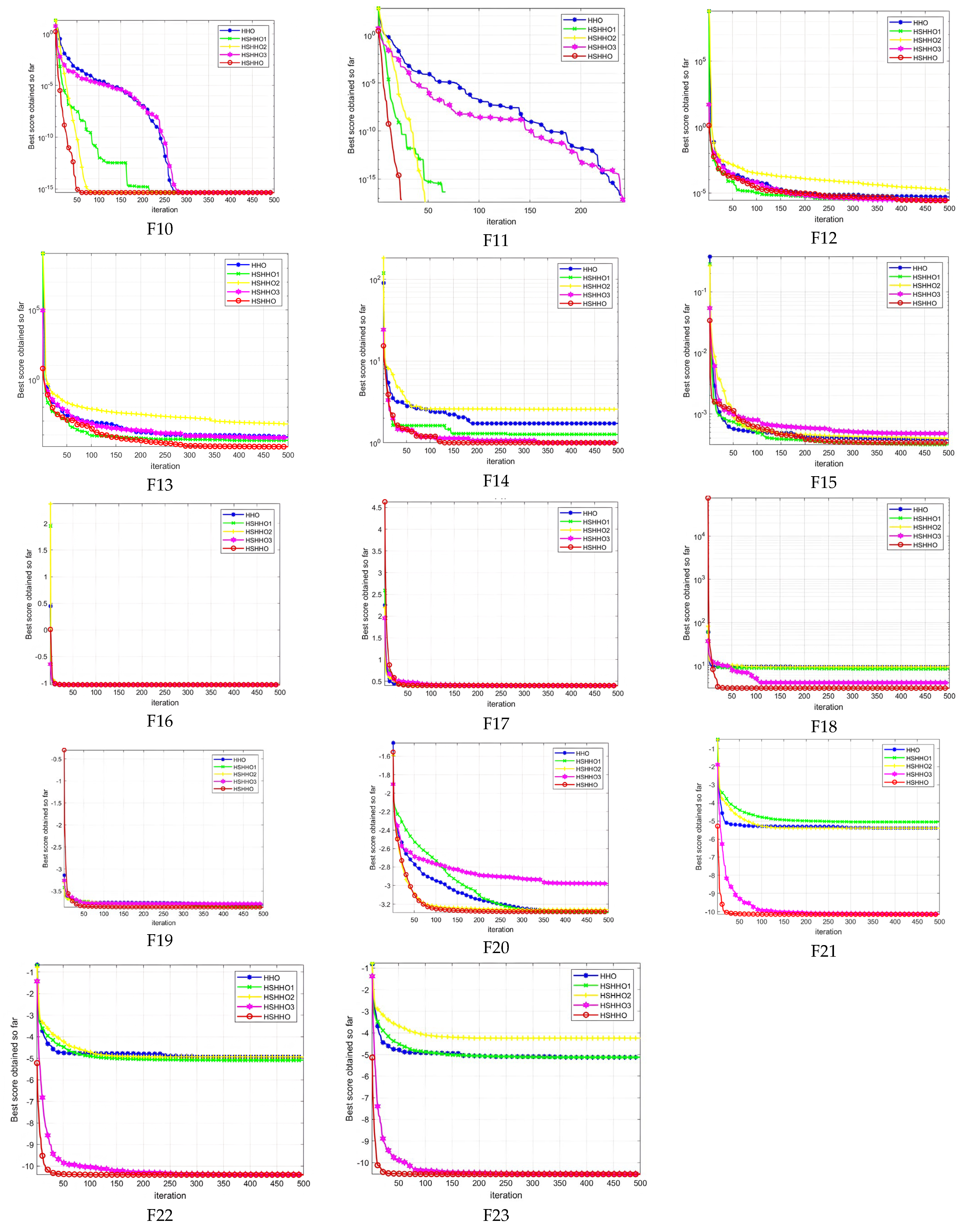
Table 2 shows the experimental results of HHO, HSHHO, and these function variants, with the optimal values displayed in bold. Figure 5 shows the convergence curves of these algorithms. Overall, the ARV in Table 2 indicates that in most tests, HSHHO and its variants perform better than HHO. This confirms the effectiveness of SPM-VLS, nonlinear escape energy, and Cauchy–Gaussian perturbation strategies in improving the quality of HHO solutions.
The Wilcoxon rank sum test in Table 3 shows significant differences between HSHHO1 and HHO in most functions. HSHHO2 performs well on eight functions, but performs poorly on F5–F8, F12–F14, and F23. This indicates that nonlinear escape energy faces difficulties in maintaining phase balance in unimodal and multimodal scenarios. However, the p-values in Table 3 indicate that all optimization strategies except F14 can improve the performance of HHO. Meanwhile, HSHHO3 ensures an optimal solution for all problems except F5, emphasizing the promoting effect of the perturbation strategy on local refinement. The p-value indicates that all functions except F6 and F12 show significance.

3.2. Comparison Between HSHHO and Other Optimization Algorithms

This section evaluates the performance comparison between HSHHO and eight popular optimization algorithms based on 30 benchmark functions of CEC 2017. Table 4 shows the description of the CEC 2017. Especially, the F2 of the CEC 2017 test function has been officially proven to have issues. However, in order to maintain the integrity and continuity of the testing, F2 is retained but not used in the experiment in this study.
Eight popular optimization algorithms include WOA, SSA, MFO, GOA, SCA, PSO, and GWO. Table 5 reports the AVG and STD metrics, with the best performers highlighted in bold. To emphasize performance differences, we applied the non-parametric Wilcoxon rank sum test, with p-values detailed in Table 6.
The unimodal benchmark has a single global optimum, making it an ideal choice for convergence speed and accuracy. According to Table 4, F1–F3 belong to this category. As shown in Table 5, HSHHO ensures the lowest AVG and STD. The p-values in Table 6 show significant differences compared to competitors on all unimodal functions. These results highlight HSHHO’s enhanced handling of unimodal challenges, thanks to the robust global exploration of the SPM-VLS strategy during the search phase.
In contrast, multimodal benchmarks contain multiple local optima, which test the algorithm’s ability to avoid getting stuck and optimize locally. The CEC 2017 test ensured comprehensive validation, improving the reliability and breadth of the experiment. Table 5 shows that HSHHO dominates all multimodal functions except for F4 and F7. However, for most functions, HSHHO exhibits significant advantages. This highlights its powerful utilization ability, which is driven by Cauchy–Gaussian elite perturbations and helps escape local minima and broader global pursuits.
To increase rigor, we studied the mixed (F11–F20) and combined (F21–F30) functions of CEC 2017, which are more complex than single or multi peak types. Table 5 confirms the highest AVG and STD of HSHHO on all functions except F17 and F27. On F17 and F27, HSHHO ranks second in value. The p-values in Table 6 confirm that they are significantly better than other algorithms on each mixing and combining function. These results stem from the nonlinear escape energy mechanism, which promotes optimal phase balance in HSHHO and produces excellent performance on complex problems.
In summary, according to the results in Table 5, HSHHO exhibits excellent performance in 26 out of 30 benchmark functions. However, according to the “no free lunch” theorem, it can be observed that HSHHO is not the optimal executor in all cases. For example, it ranks second on functions F4, F7, F17, and F27 or is comparable to GWO and SSA. This indicates that although HSHHO has strong robustness to mixing and combining problems, specific landscape features in certain multimodal functions may still be more effectively navigated through other metaheuristic methods.
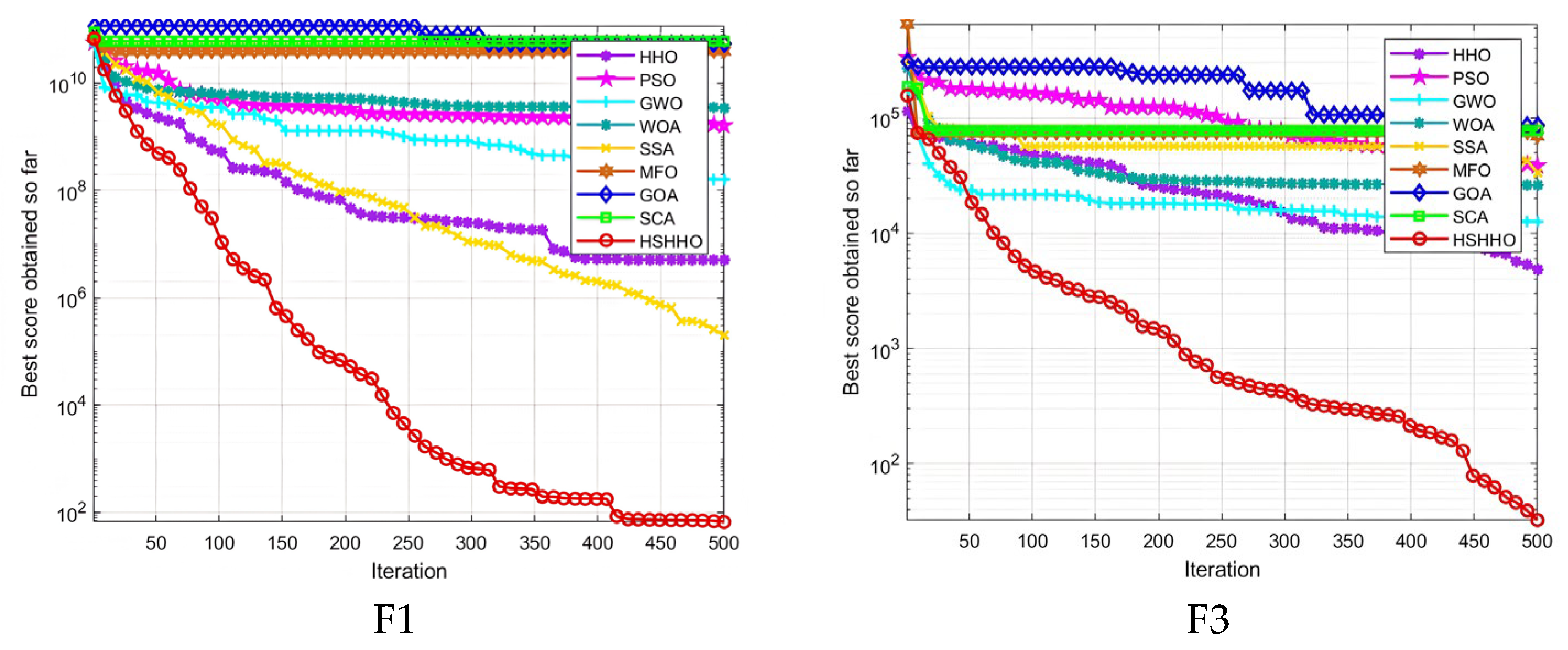
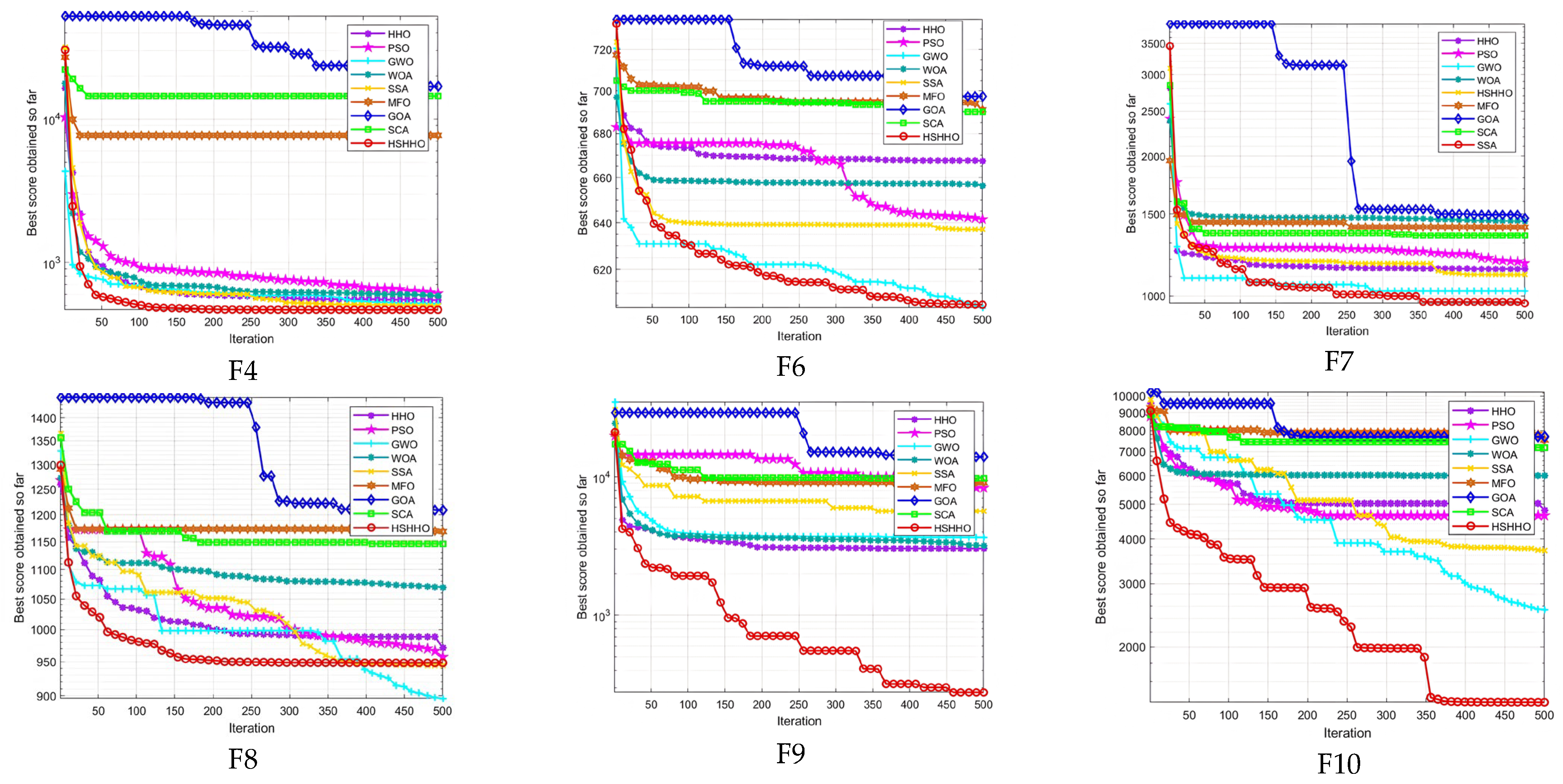
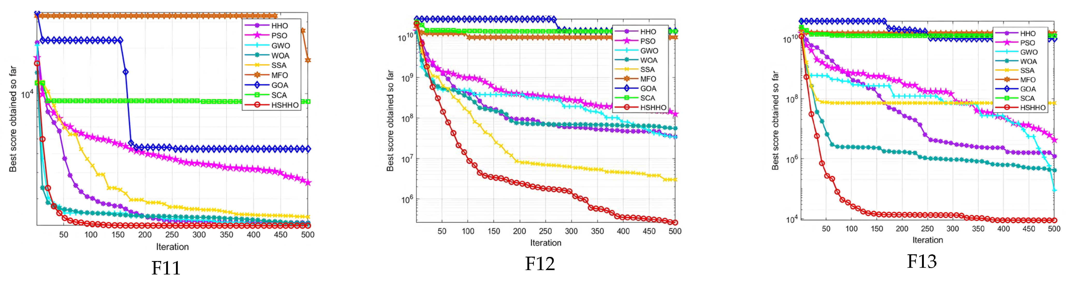
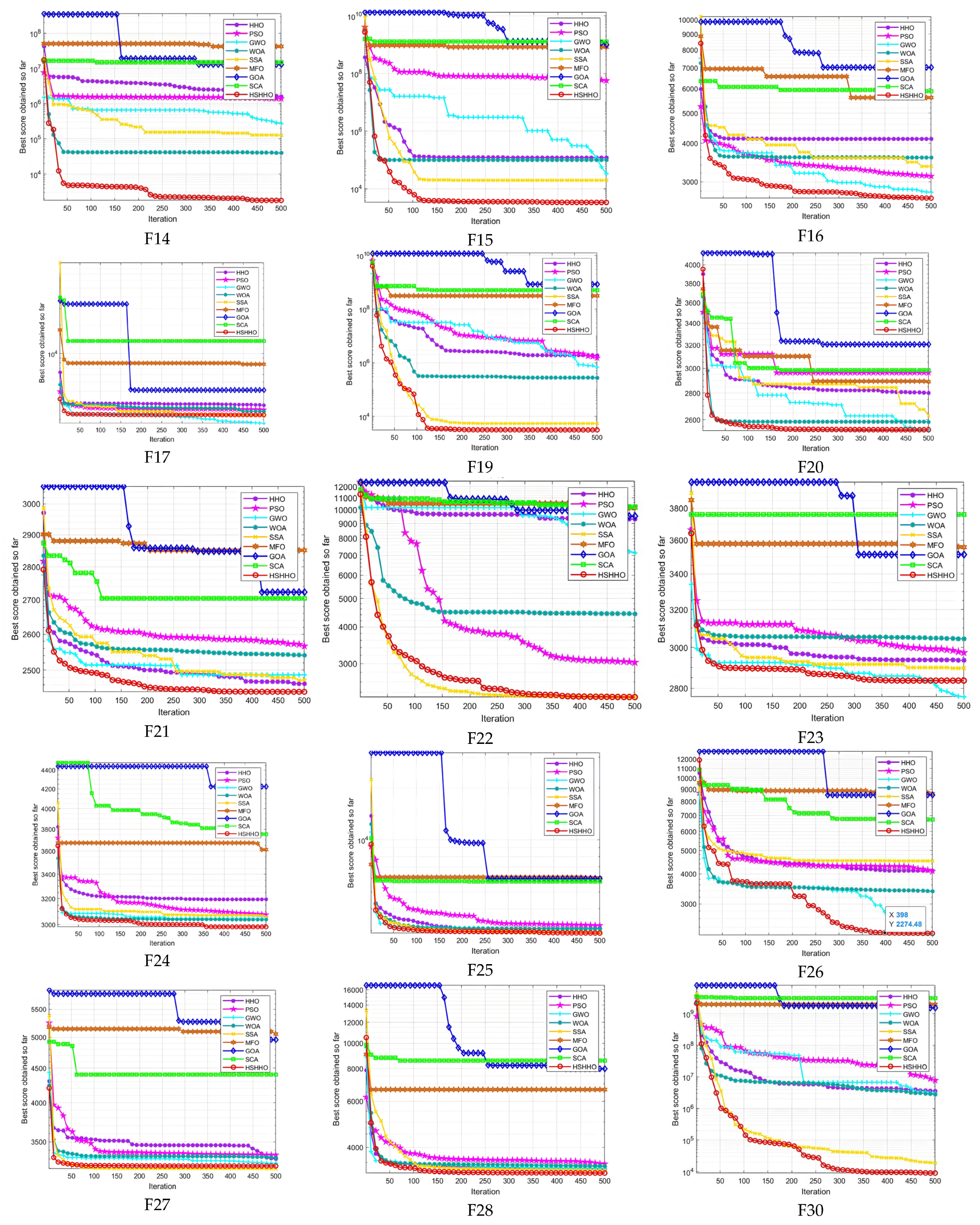
The convergence graph in Figure 6, Figure 7 and Figure 8 visually compares HSHHO with different optimization algorithms. Figure 6 depicts the rapid decline and sustained accuracy advantage of HSHHO. Figure 7 shows that HSHHO quickly reaches its optimal value, surpassing other algorithms. Figure 8 highlights the leading speed of HSHHO on all functions except F22, ultimately achieving unparalleled accuracy.
In addition, we compare the average time. According to Table 7, PSO and WOA achieved good results on the benchmark test function. Compared with HHO, the average time of HSHHO increased due to the influence of three improvement strategies. However, achieving better computational results at a smaller time cost is often acceptable.

3.3. HSHHO for Feature Selection

To demonstrate the practical value of HSHHO, we apply it to feature selection tasks spanning datasets with feature counts ranging from a few to several hundred. Its performance is benchmarked against several established metaheuristic algorithms.

3.3.1. Datasets and Parameter Settings

We selected 18 widely used UCI datasets, detailed in Table 8, that have been extensively validated in prior feature selection research, ensuring both reliability and relevance.
Using the wrapper approach, the optimizer is combined with the classifier to identify the optimal feature subset. In order to evaluate the accuracy of the selected feature subset, a classifier must be used for classification after feature selection. The KNN classifier is a popular classification method in the field of feature selection. The selection of K value and distance measurement in KNN affect the effectiveness of KNN. In this study, the selection of K value refers to the existing literature, with a value of 5 [49]. For each dataset, the samples are divided into 80% training set and 20% testing set, and reliability is improved through 10-fold cross validation. All experiments were repeated 10 times to eliminate the influence of random fluctuations.
For comparative analysis, HSHHO is tested alongside HHO, PSO, GWO, WOA, SSA, and GOA. Common parameters are fixed as follows: population size = 10, maximum iterations = 100, and search dimension equal to the number of features in each dataset. The parameters of each algorithm are summarized in Table 9. All implementations are developed and executed in MATLAB R2022b.

3.3.2. Performance Indicators

To evaluate the performance of the HSHHO, three statistical indicators are introduced, including average fitness, average accuracy, and average feature selection size.
  • Average fitness (AvgFit): Average value of the fitness obtained.
    A v g F i t = 1 T i = 1 T F i t b e s t i
    where  F i t b e s t i  denotes the best fitness obtained in the  i -th iteration.
  • Average accuracy (AvgAcc): Accuracy of the classifier in selecting the best feature subset.
    A v g A c c = 1 T i = 1 T A c c i
    where  A c c i  is the accuracy achieved by the optimal subset in the  i -th iteration.
  • Average number of feature selections (AvgSel): Average value of the ratio of the number of features selected.
    A v g S e l = 1 T i = 1 T F S n u m b e r i D
    where  F S n u m b e r i  the number of features selected in the  i -th iteration, and  D  is the total number of original features.
  • Average run-time (AvgRt): Average value of the algorithm’s run time.
    A v g R t = 1 T i = 1 T T i m e i
    where  T i m e i  denotes the run time in the  i -th iteration.

3.3.3. Comparison Results on the 18 Feature Datasets

For average fitness, the results are reported in Table 10. According to Table 10, it can be observed that HSHHO obtains the best value on the 16-feature datasets. Compared to HHO, PSO, GWO and WOA, HSHHO achieves the best results on all datasets. SSA achieves the optimal fitness value on the WaveformEW dataset, while GOA achieves better results on the Vote dataset.
For average accuracy, the results are reported in Table 11. It is evident that HSHHO demonstrates superior performance. Compared to SSA, HSHHO also achieves the best results on other datasets except the HeartEW, IonosphereEW, and WaveformEW datasets. For PSO, GWO, and GOA, HSHHO achieves the best results on all datasets. Additionally, SSA ranks second for accuracy.
In terms of the number of selected features, based on the average number of selected features by HSHHO and other optimization algorithms reported in Table 12, it can be observed that, compared to the standard HHO, HSHHO obtains the minimum number of selected features on all 18-feature datasets. Compared to GWO, HSHHO obtains the best feature subset on all datasets except the KrvskpEW dataset. SSA obtains the least number of features on the SonarEW and PenglungEW datasets. The GOA finds the optimal number of selected features on the WaveformEW dataset. In total, HSHHO finds the best feature subsets on 14 datasets (Exactly, Exactly2, Breastcancer, Lymphography, Vote, Zoo, BreastEW, CongressEW, HeartEW, IonosphereEW, WineEW, SpectEW, Tic-tac-toe and PenglungEW), and the number of features obtained on the remaining four datasets ranked second.
For average accuracy, the results are reported in Table 13. It is evident that HSHHO demonstrates superior performance. Compared to SSA, HSHHO also achieves the best results on other datasets except the HeartEW, IonosphereEW, and WaveformEW datasets. For PSO, GWO, and GOA, HSHHO achieves the best results on all datasets. Additionally, SSA ranks second for accuracy.
In addition, Table 13 provides detailed information on the average time. The analysis of experimental results shows that, compared with other algorithms, the proposed method requires the longest time. This is due to the introduction of three improvement strategies, which extend the time required to mine the optimal solution. When used for FS, the number of features is a dimension, and the higher the dimension, the longer the required time. Although PSO and WOA require the shortest time in the dataset, their classification accuracy is not the highest and they cannot minimize the number of features. Therefore, considering other metrics, HSHHO still outperforms other algorithms in terms of FS.

3.3.4. Comprehensive Correlation Analysis

To evaluate whether the improvement of fitness is essentially based on classification performance, a three indicators correlation analysis was conducted on Table 8, Table 9 and Table 10. Firstly, the comparison between fitness and accuracy indicates that the optimization of HSHHO is performance-oriented. In 16 out of 18 datasets, a decrease in fitness values was accompanied by a significant increase in accuracy. It is worth noting that on high-dimensional datasets such as KrvskpEW and PenglingEW, HSHHO achieved excellent accuracy while significantly reducing fitness scores. This confirms that the fitness function effectively captures the algorithm’s ability to enhance discriminative power. Secondly, the relationship between accuracy and feature subset size indicates the efficiency of HSHHO in noise filtering. According to Table 10, HSHHO achieved a smaller feature subset than HHO in all 18 datasets. In most cases, a decrease in the feature count leads to a reverse improvement in accuracy, indicating that the eliminated features are mainly redundant or noisy.
In addition to solving quality, the practical usability of the proposed HSHHO framework should also be evaluated based on computational costs. Since HSHHO incorporates three improvement strategies, its processing naturally requires more time than the original HHO. Therefore, the runtime results should be interpreted in conjunction with accuracy results rather than in isolation.
According to Table 7 and Table 13, we can observe that on the feature selection dataset, the average computation time increased from 597.67 s for HHO to 630.35 s for HSHHO; on the benchmark functions, it rose from 16.54 s for HHO to 22.24 s. Although this indicates an increase in computational cost, HSHHO demonstrates superior algorithmic performance.
These results indicate that the additional runtime of HSHO is associated with improved search quality and stronger convergence behavior, rather than an unnecessary computational burden. In other words, HSHO achieves higher optimization accuracy, enhanced robustness, and more reliable final solutions at the cost of a moderate additional runtime. This trade-off is advantageous in applications where solution quality and stability are more critical than minimal execution time. In summary, the improved HSHHO fitness is a collaborative result of achieving higher classification accuracy with a more concise feature set.

4. Conclusions

In this paper, we introduce an enhanced Harris Hawks Optimization algorithm, named HSHHO, which incorporates the SPM with variable logarithmic spiral, nonlinear escape energy mechanism, and Cauchy–Gaussian elite perturbation. By integrating these enhancements, HSHHO improves initial population diversity, global search efficiency, and local refinement accuracy. To evaluate its effectiveness, we first examined the impact of the three strategies on HHO that use 23 classical benchmark functions, revealing that each contributes meaningfully to overall improvement. Next, IEEE CEC 2017 is used to compare HSHHO with eight well-known algorithms. The results indicate that HSHHO dominates a significant competitive advantage at most benchmark functions. Finally, when applied to 18 feature selection tasks, HSHHO delivered outstanding results, notably reducing feature counts by 70.92% while elevating average classification accuracy to 94.47%.
Although HSHHO has demonstrated strong optimization capabilities, the inherent limitations in hybrid strategies need to be addressed. The integration of SPM chaotic mapping and Cauchy–Gaussian mutation significantly improves the search performance of the algorithm, but also enhances its sensitivity by increasing the initial parameter configuration. Meanwhile, experimental results indicate that HSHHO dominates in most benchmark tests, but its performance in specific functions still needs improvement. In addition, the transition between exploration and mining may still experience local stagnation, indicating that a single nonlinear energy model may not be universally applicable to all complex multimodal problems.
From these insights, several avenues for future exploration have emerged. Firstly, the development phase can be improved by integrating search operators from alternative optimizers. Secondly, its application may be extended to real engineering problems, such as railway emergency scenario prediction, medical big data analysis, intelligent risk assessment, etc. Thirdly, future research will compare HSHHO with the latest feature selection algorithms and continuously optimize algorithm performance. In addition, a notable prospect lies in developing a unified framework to interactively orchestrate multiple metaheuristics and machine learning models, leveraging their collective strengths to tackle daunting real-world challenges and generate higher-quality solutions. On the basis of this project, we will improve the HSHHO algorithm and apply it to key point recognition in typical emergency response scenarios of railways. By identifying the core feature subset in the collaborative emergency process of multiple disciplines, a scientific method is provided for railway emergency response operation standards, and an important role is played in risk warning and emergency plan optimization.


Author Contributions

Conceptualization, G.L. and X.L.; methodology, G.L. and X.L.; software, G.L. and R.Y.; validation, R.Y.; formal analysis, X.L.; writing—original draft preparation, G.L.; writing—review and editing, G.L. and R.Y.; supervision, X.L. All authors have read and agreed to the published version of the manuscript.

Funding

This work was funded by the China State Railway Group Co., Ltd. Science and Technology Research and Development Plan Project, grant number [2025F028]; China Academy of Railway Sciences Research Fund, grant number [2025YJ092].

Data Availability Statement

The original contributions presented in this study are included in the article. Further inquiries can be directed to the corresponding author.

Conflicts of Interest

Author Guanyi Liu was employed by the company China Academy of Railway Sciences Corporation Limited. The remaining authors declare that the research was conducted in the absence of any commercial or financial relationships that could be construed as a potential conflict of interest. The authors declare that this study received funding from China State Railway Group Co., Ltd. The funder was not involved in the study design, collection, analysis, interpretation of data, the writing of this article or the decision to submit it for publication.

References

  1. Mach-Król, M. On a certain research gap in big data mining for customer insights. Appl. Sci. 2021, 11, 6993. [Google Scholar] [CrossRef] [Scilit]
  2. Lohrmann, C.; Lohrmann, A.; Kumbure, M.M. On the benefit of feature selection and ensemble feature selection for fuzzy k-nearest neighbor classification. Appl. Soft. Comput. 2025, 171, 112784. [Google Scholar] [CrossRef] [Scilit]
  3. Keerthana, G.; Annabel, L.S.P. A survey on big data classification. Data Knowl. Eng. 2025, 156, 102408. [Google Scholar] [CrossRef] [Scilit]
  4. Gurcan, F.; Gudek, B.; Dalveren, G.G.M.; Derawi, M. Future-Ready skills across big data ecosystems: Insights from machine learning-driven human resource analytics. Appl. Sci. 2025, 15, 5841. [Google Scholar] [CrossRef] [Scilit]
  5. Nogueira, A.R.; Pugnana, A.; Ruggieri, S.; Pedreschi, D.; Gama, J. Methods and tools for causal discovery and causal inference. Wiley Interdiscip. Rev. Data Min. Knowl. Discov. 2022, 12, e1449. [Google Scholar] [CrossRef] [Scilit]
  6. Zhang, Y.; Liu, R.; Wang, X.; Chen, H.L. Boosted binary Harris hawks optimizer and feature selection. Eng. Comput. 2021, 37, 3741–3770. [Google Scholar] [CrossRef] [Scilit]
  7. Bharti, K.K.; Singh, P.K. Opposition chaotic fitness mutation based adaptive inertia weight BPSO for feature selection in text clustering. Appl. Soft Comput. 2016, 43, 20–34. [Google Scholar] [CrossRef] [Scilit]
  8. Yang, X.X.; Liu, J.; Liu, Y.; Xu, P.; Yu, L.; Zhu, L.; Chen, H.Y.; Deng, W. A novel adaptive sparrow search algorithm based on chaotic mapping and T-distribution mutation. Appl. Sci. 2021, 11, 11192. [Google Scholar] [CrossRef] [Scilit]
  9. Shan, W.F.; He, X.X.; Liu, H.J.; Heidari, A.A.; Wang, M.F.; Cai, Z.N.; Chen, H.L. Cauchy mutation boosted Harris hawk algorithm: Optimal performance design and engineering applications. J. Comput. Des. Eng. 2023, 10, 503–526. [Google Scholar] [CrossRef] [Scilit]
  10. Gundluru, N.; Rajput, D.S.; Lakshmanna, K.; Kaluri, R.; Shorfuzzaman, M.; Uddin, M.; Khan, M.A.R. Enhancement of Detection of Diabetic Retinopathy Using Harris Hawks Optimization with Deep Learning Model. Comput. Intell. Neurosci. 2022, 2022, 8512469. [Google Scholar] [CrossRef] [Scilit]
  11. Liu, K.Z.; Dai, Y.Q.; Liu, H. Improvement of Dung Beetle Optimization Algorithm Application to Robot Path Planning. Appl. Sci. 2025, 15, 396. [Google Scholar] [CrossRef] [Scilit]
  12. Mohamed, B.; Mohaisen, L.; Amin, M. Computing Connected Resolvability of Graphs Using Binary Enhanced Harris Hawks Optimization. Intell. Autom. Soft Comput. 2023, 36, 2349–2361. [Google Scholar] [CrossRef] [Scilit]
  13. Gupta, A.; Chhikara, R.; Sharma, P. An improved continuous and discrete Harris Hawks optimiser applied to feature selection for image steganalysis. Int. J. Comput. Sci. Eng. 2024, 27, 515–535. [Google Scholar] [CrossRef] [Scilit]
  14. Özbay, F.A. An enhanced zebra optimization algorithm with multiple strategies for global optimization and feature selection problems: A hepatocellular carcinoma case study. IEEE Access 2025, 13, 30036–30057. [Google Scholar] [CrossRef] [Scilit]
  15. Li, J.; Sun, K.X. Pressure vessel design problem using improved gray wolf optimizer based on cauchy distribution. Appl. Sci. 2023, 13, 12290. [Google Scholar] [CrossRef] [Scilit]
  16. Wen, L.; Wang, G.P.; Yue, L.W.; Liang, X.D.; Chen, H.N. Multistrategy Harris Hawks Optimization Algorithm Using Chaotic Method, Cauchy Mutation, and Elite Individual Guidance. Discret. Dyn. Nat. Soc. 2022, 2022, 5129098. [Google Scholar] [CrossRef] [Scilit]
  17. Sun, Y.S.; Huang, Q.; Liu, T.; Cheng, Y.T.; Li, Y.Q. Multi-strategy enhanced harris hawks optimization for global optimization and deep learning-based channel estimation problems. Mathematics 2023, 11, 390. [Google Scholar] [CrossRef] [Scilit]
  18. Chen, X.L.; Qin, H.; Liu, S.; Chen, J.W.; Li, Y.X.; Zhu, X. Intelligent Scheduling Method for Cascade Reservoirs Driven by Dual Optimization of Harris Hawks and Marine Predators. Water 2025, 17, 3291. [Google Scholar] [CrossRef] [Scilit]
  19. Long, W.; Jiao, J.J.; Xu, M.; Tang, M.Z.; Wu, T.B.; Cai, S.H. Lens-imaging learning Harris hawks optimizer for global optimization and its application to feature selection. Expert Syst. Appl. 2022, 204, 117555. [Google Scholar] [CrossRef] [Scilit]
  20. Saelee, J.; Wetchapram, P.; Wanichsombat, A.; Intarasit, A.; Muangprathub, J.; Boongasame, L.; Choopradit, B. Enhanced Feature Selection via Hierarchical Concept Modeling. Appl. Sci. 2024, 14, 10965. [Google Scholar] [CrossRef] [Scilit]
  21. Ding, J.Y.; Du, J.C.; Wang, H.J.; Xiao, S. A novel two-stage feature selection method based on random forest and improved genetic algorithm for enhancing classification in machine learning. Sci. Rep. 2025, 15, 16828. [Google Scholar] [CrossRef] [Scilit]
  22. Zhao, M.; Ye, N. FS-SVM: High-Dimensional Ensemble Learning Classification: An Ensemble Learning Classification Algorithm Based on High-Dimensional Feature Space Reconstruction. Appl. Sci. 2024, 14, 1956. [Google Scholar] [CrossRef] [Scilit]
  23. Yang, K.K.; Liu, L.; Wen, Y.L. The impact of Bayesian optimization on feature selection. Sci. Rep. 2024, 14, 3948. [Google Scholar] [CrossRef] [Scilit] [PubMed]
  24. Zhang, M.L.; Peña, J.M.; Robles, V. Feature selection for multi-label naive Bayes classification. Inf. Sci. 2009, 179, 3218–3229. [Google Scholar] [CrossRef] [Scilit]
  25. Gbashi, S.M.; Adedeji, P.A.; Olatunji, O.O.; Madushele, N. Optimal feature selection for a weighted k-nearest neighbors for compound fault classification in wind turbine gearbox. Results Eng. 2025, 25, 103791. [Google Scholar] [CrossRef] [Scilit]
  26. Nemati, K.; Sheikhani, A.H.R.; Kordrostami, S.; Roudposhti, K.K. New Hybrid Feature Selection Approaches Based on ANN and Novel Sparsity Norm. J. Electr. Comput. Eng. 2024, 2024, 7112770. [Google Scholar] [CrossRef] [Scilit]
  27. Passemiers, A.; Folco, P.; Raimondi, D.; Birolo, G.; Moreau, Y.; Fariselli, P. A quantitative benchmark of neural network feature selection methods for detecting nonlinear signals. Sci. Rep. 2024, 14, 31180. [Google Scholar] [CrossRef] [Scilit]
  28. Xiao, J.E.; Hong, M. A Feature Selection Method Based on a Convolutional Neural Network for Text Classification. Electronics 2025, 14, 4615. [Google Scholar] [CrossRef] [Scilit]
  29. Xu, Y.T.; Chen, H.L.; Heidari, A.A.; Luo, J.; Zhang, Q.; Zhao, X.H.; Li, C.Y. An efficient chaotic mutative moth- flame-inspired optimizer for global optimization tasks. Expert Syst. Appl. 2019, 129, 135–155. [Google Scholar] [CrossRef] [Scilit]
  30. Emary, E.; Zawbaa, H.M.; Sharawi, M. Impact of Levy flight on modern meta-heuristic optimizers. Appl. Soft. Comput. 2019, 75, 775–789. [Google Scholar] [CrossRef] [Scilit]
  31. Shen, C.N.; Zhang, K. Two-stage improved grey wolf optimization algorithm for feature selection on high-dimensional classification. Complex Intell. Syst. 2022, 8, 2769–2789. [Google Scholar] [CrossRef] [Scilit]
  32. Mirjalili, S.; Saremi, S.; Mirjalili, S.M.; Coelho, L.D. Multi-objective grey wolf optimizer: A novel algorithm for multi-criterion optimization. Expert Syst. Appl. 2016, 47, 106–119. [Google Scholar] [CrossRef] [Scilit]
  33. Adegboye, O.R.; Feda, A.K.; Ojekemi, O.S.; Agyekum, E.B.; Hussien, A.G.; Kamel, S. Chaotic opposition learning with mirror reflection and worst individual disturbance grey wolf optimizer for continuous global numerical optimization. Sci. Rep. 2024, 14, 4660. [Google Scholar] [CrossRef] [Scilit]
  34. Liu, X.L.; Tian, H.W. A novel hybrid feature selection method combining binary grey wolf optimization and cuckoo search. Sci. Rep. 2025, 15, 45190. [Google Scholar] [CrossRef] [Scilit] [PubMed]
  35. Al-Tashi, Q.; Abdulkadir, S.J.; Rais, H.M.; Mirjalili, S.; Alhussian, H. Binary optimization using hybrid grey wolf optimization for feature selection. IEEE Access 2019, 7, 39496–39508. [Google Scholar] [CrossRef] [Scilit]
  36. Hassan, B.A. CSCF: A chaotic sine cosine firefly algorithm for practical application problems. Neural Comput. Appl. 2021, 33, 7011–7038. [Google Scholar] [CrossRef] [Scilit]
  37. Garg, H. A hybrid GSA-GA algorithm for constrained optimization problems. Inf. Sci. 2019, 478, 499–523. [Google Scholar] [CrossRef] [Scilit]
  38. Li, M.W.; Wang, Y.T.; Geng, J.; Hong, W.C. Chaos cloud quantum bat hybrid optimization algorithm. Nonlinear Dyn. 2021, 103, 1167–1193. [Google Scholar] [CrossRef] [Scilit]
  39. Ibrahim, R.A.; Abd Elaziz, M.; Oliva, D.; Cuevas, E.; Lu, S.F. An opposition-based social spider optimization for feature selection. Soft. Comput. 2019, 23, 13547–13567. [Google Scholar] [CrossRef] [Scilit]
  40. Heidari, A.A.; Mirjalili, S.; Faris, H.; Aljarah, I.; Mafarja, M.; Chen, H. Harris hawks optimization: Algorithm and applications. Future Gener. Comput. Syst. 2019, 97, 849–872. [Google Scholar] [CrossRef] [Scilit]
  41. Jiao, S.B.; Wang, C.; Gao, R.; Li, Y.X.; Zhang, Q. Harris Hawks Optimization with multi-strategy search and application. Symmetry 2021, 13, 2364. [Google Scholar] [CrossRef] [Scilit]
  42. Long, W.; Jiao, J.J.; Liang, X.M.; Tang, M.Z. An exploration-enhanced grey wolf optimizer to solve high-dimensional numerical optimization. Eng. Appl. Artif. Intell. 2018, 68, 63–80. [Google Scholar] [CrossRef] [Scilit]
  43. Zhang, Z.R.; Huang, H.Q.; Huang, C.Q.; Han, B. An improved TLBO with logarithmic spiral and triangular mutation for global optimization. Neural Comput. Appl. 2019, 31, 4435–4450. [Google Scholar] [CrossRef] [Scilit]
  44. Mondal, B.; Singh, S.; Kumar, P. A secure image encryption scheme based on cellular automata and chaotic skew tent map. J. Inf. Secur. Appl. 2019, 45, 117–130. [Google Scholar] [CrossRef] [Scilit]
  45. Wu, Y.B.; Sun, D.F.; Zhang, M.J.; Zhao, J.Y.; Wu, H.F. Beetle swarm with constrained levy flight for image matching. IEEE Trans. Autom. Sci. Eng. 2025, 22, 3366–3376. [Google Scholar] [CrossRef] [Scilit]
  46. Almotairi, S.; Alqahtani, A.; Alkhaldi, A.; Alshathri, S.; Alhenawi, E. Three chaotic strategies for enhancing the self-adaptive Harris Hawk optimization algorithm for global optimization. Mathematics 2023, 11, 4181. [Google Scholar] [CrossRef] [Scilit]
  47. Mirjalili, S.; Gandomi, A.H.; Mirjalili, S.Z.; Saremi, S.; Faris, H.; Mirjalili, S.M. Salp swarm algorithm: A bio-inspired optimizer for engineering design problems. Adv. Eng. Softw. 2017, 114, 163–191. [Google Scholar] [CrossRef] [Scilit]
  48. Zhu, Y.B.; Li, T.; Lan, X.L. Feature selection optimized by the artificial immune algorithm based on genome shuffling and conditional lethal mutation. Appl. Intell. 2023, 53, 13972–13992. [Google Scholar] [CrossRef] [Scilit]
  49. Tamara, A.Q.; Mohd, M.N.; Mohammed, A.B.; Ahamad, T.K. Improved gray wolf harris hawk algorithm based feature selection for sentiment analysis. Results Control Optim. 2025, 20, 100604. [Google Scholar] [CrossRef] [Scilit]
Figure 1. Different stages of HHO.
Applsci 16 06488 g001
Figure 2. Population distribution diagrams of SPM.
Applsci 16 06488 g002
Figure 3. Histograms of distributions of SPM.
Applsci 16 06488 g003
Figure 4. Flowchart of the HSHHO algorithm.
Applsci 16 06488 g004
Figure 5. Convergence curves on 23 classical benchmark functions.
Applsci 16 06488 g005aApplsci 16 06488 g005b
Figure 6. Convergence curves on unimodal benchmark functions.
Applsci 16 06488 g006
Figure 7. Convergence curves on multimodal benchmark functions.
Applsci 16 06488 g007
Figure 8. Convergence curves on hybrid and composition benchmark functions.
Applsci 16 06488 g008aApplsci 16 06488 g008b
Table 1. Descriptions of the 23 standard benchmark functions.
FunctionDimRangeOptimumClass
F 1 ( x ) = i = 1 n x i 2 30[−100, 100]0Unimodal benchmark functions
F 2 ( x ) = i = 1 n x i + i = 1 n x i 30[−10, 10]0
F 3 ( x ) = i = 1 n j 1 i x j 2 30[−100, 100]0
F 4 ( x ) = m a x i x i , 1 i n 30[−100, 100]0
F 5 ( x ) = i = 1 n 1 100 x i + 1 x i 2 2 + x i 1 2 30[−30, 30]0
F 6 ( x ) = i = 1 n x i + 0.5 2 30[−100, 100]0
F 7 ( x ) = i = 1 n i x i 4 + r a n d o m [ 0 , 1 ] 30[−1.28, 1.28]0
F 8 ( x ) = i = 1 n x i s i n x i 30[−500, 500] 418.98 × D i m Multimodal benchmark functions
F 9 ( x ) = i = 1 n x i 2 10 c o s 2 π x i + 10 30[−5.12, 5.12]0
F 10 x = 20 e x p 0.2 1 n i = 1 n x i 2 e x p 1 n i = 1 n cos 2 π x i + 20 + e 30[−32, 32]0
F 11 x = 1 4000 i = 1 n x i 2 i = 1 n c o s x i i + 1 30[−600, 600]0
F 12 x = π n 10 s i n π y i + i = 1 n 1 y i 1 2 1 + 10 s i n 2 π y i + 1 + y n 1 2 + i = 1 n u ( x i , 10 , 100 , 4 )
y i = 1 + x i + 1 4
u x i , a , k , m = k ( x i a ) m                   x i > a 0                           a < x i < a k ( x i a ) m       x i < a
30[−50, 50]0
F 13 x = 0.1 s i n 2 3 π x 1 + i = 1 n x i 1 2 1 + s i n 2 3 π x 1 + 1 + x n 1 2 1 + s i n 2 2 π x n + i = 1 n u x i , 5 , 100 , 4 30[−50, 50]0
F 14 x = 1 500 + j = 1 25 1 j + i = 1 2 x i a i j 6 1 2[−65, 65]1Fixed-dimension multimodal benchmark functions
F 15 x = i = 1 11 a i x 1 ( b i 2 + b 1 x 2 ) b i 2 + b i x 3 + x 4 2 4[−5, 5]0.00030
F 16 x = 4 x 1 2 2.1 x 1 2 + 1 3 x 1 6 + x 1 x 2 4 x 2 2 + 4 x 2 4 2[−5, 5]−1.0316
F 17 x = x 2 5.1 4 π 2 x 1 2 + 5 π x 1 6 2 + 10 1 1 8 π c o s x 1 + 10 2[−5, 5]0.398
F 18 x = 1 + ( x 1 + x 2 + 1 ) 2 19 14 x 1 + 3 x 1 2 14 x 2 + 6 x 1 x 2 + 3 x 2 2 × 30 + 2 x 1 3 x 2 2 18 32 x 1 + 12 x 1 2 + 48 x 2 36 x 1 x 2 + 27 x 2 2 2[−2, 2]3
F 19 x = i = 1 4 c i e x p j = 1 3 a i j x j p i j 2 3[1, 3]−3.86
F 20 x = i = 1 4 c i e x p j = 1 6 a i j x j p i j 2 6[0, 1]−3.32
F 21 x = i = 1 5 X a i X a i T + c i 1 4[0, 10]−10.1532
F 22 x = i = 1 7 X a i X a i T + c i 1 4[0, 10]−10.4028
F 23 x = i = 1 10 X a i X a i T + c i 1 4[0, 10]−10.5363
Table 2. Experimental results.
FunctionIndexHHOHSHHO1HSHHO2HSHHO3HSHHO
F1AVG9.2202 × 10−941.9297 × 10−1091.6754 × 10−1422.3264 × 10−2840.0000
STD5.0487 × 10−931.0565 × 10−1089.1533 × 10−1420.00000.0000
F2AVG3.0247 × 10−501.2447 × 10−565.5461 × 10−763.0287 × 10−1400.0000
STD1.0607 × 10−496.1266 × 10−562.1252 × 10−751.6589 × 10−1390.0000
F3AVG8.1637 × 10−781.7914 × 10−943.7932 × 10−1003.0046 × 10−2860.0000
STD4.0442 × 10−779.5497 × 10−942.0373 × 10−990.00000.0000
F4AVG6.1139 × 10−486.6739 × 10−551.0344 × 10−712.7746 × 10−1440.0000
STD3.3448 × 10−472.5437 × 10−545.6653 × 10−711.5197 × 10−1430.0000
F5AVG7.4754 × 10−35.1007 × 10−32.77181.2976 × 10−23.1645 × 10⁻³
STD9.9405 × 10−37.0617 × 10−38.23812.2918 × 10−25.4109 × 10⁻³
F6AVG1.1492 × 10−45.4432 × 10−57.8722 × 10−42.4963 × 10−51.4019 × 10−5
STD1.1033 × 10−41.3313 × 10−43.9139 × 10−44.8599 × 10−51.8865 × 10−5
F7AVG1.4853 × 10−41.1531 × 10−42.9132 × 10−41.0458 × 10−46.9998 × 10−5
STD1.5813 × 10−49.0161 × 10−57.5267 × 10−41.2357 × 10−46.4866 × 10−5
F8AVG−1.2568 × 10⁴−1.2568 × 10⁴−1.1717 × 10⁴−1.2541 × 10⁴−1.2507 × 10⁴
STD8.5821 × 10−11.83052.1650 × 1039.7629 × 1013.1601 × 102
F9AVG0.00000.00000.00000.00000.0000
STD0.00000.00000.00000.00000.0000
F10AVG4.4409 × 10−164.4409 × 10−164.4409 × 10−164.4409 × 10−164.4409 × 10⁻¹⁶
STD0.00000.00000.00000.00000.0000
F11AVG0.00000.00000.00000.00000.0000
STD0.00000.00000.00000.00000.0000
F12AVG5.0048 × 10−63.0985 × 10−61.5908 × 10−52.9053 × 10−62.6737 × 10−6
STD7.5440 × 10−65.2977 × 10−68.1661 × 10−68.7679 × 10−66.2248 × 10−6
F13AVG7.3854 × 10−54.1608 × 10−56.1878 × 10−46.4770 × 10−51.4577 × 10−5
STD1.0268 × 10−45.3595 × 10−52.0259 × 10−31.6530 × 10−42.6671 × 10−5
F14AVG1.72301.26262.56989.9800 × 10−19.9800 × 10⁻¹
STD1.48666.8599 × 10−12.92061.9366 × 10−61.5070 × 10⁻⁷
F15AVG3.7550 × 10−43.1184 × 10−43.9282 × 10−44.7645 × 10−43.3515 × 10−4
STD3.4535 × 10−41.0682 × 10−53.1044 × 10−43.4231 × 10−42.6490 × 10−5
F16AVG−1.0316−1.0316−1.0316−1.0316−1.0316
STD9.9897 × 10−103.6767 × 10−103.0363 × 10−101.8941 × 10−56.0994 × 10−6
F17AVG3.9789 × 10−13.9789 × 10−13.9789 × 10−13.9789 × 10−13.9789 × 10−1
STD7.8303 × 10−75.5480 × 10−73.2770 × 10−44.9781 × 10−41.1796 × 10−7
F18AVG9.30008.40009.30003.98763.0000
STD1.1615 × 1011.0984 × 1011.1615 × 1015.40513.7568 × 10−8
F19AVG−3.8112−3.0897−3.0898−3.6037−3.8615
STD1.9611 × 10−13.1446 × 10−12.3587 × 10−19.3659 × 10−21.8628 × 10−3
F20AVG−3.2858−3.2929−3.2584−2.9789−3.2823
STD5.5976 × 10−15.3445 × 10−16.0406 × 10−11.5164 × 10−15.7081 × 10−2
F21AVG−5.395−5.0548−5.395−1.0129 × 101−1.0152 × 101
STD1.29338.1976 × 10−51.29343.9687 × 10−23.1446 × 10⁻³
F22AVG−4.9338−5.0876−4.9313−1.0383 × 101−1.0402 × 101
STD6.3550 × 10−14.9794 × 10−51.88833.3322 × 10−23.7548 × 10⁻⁴
F23AVG−5.1282−5.1284−4.2499−1.0510 × 101−1.0535 × 101
STD1.23035.4647 × 10−51.80404.1428 × 10−27.4586 × 10⁻⁴
Bold represents the optimal value.
Table 3. The p-values of the Wilcoxon rank-sum test with 5% significance of experimental results.
FunctionHHOHSHHO1HSHHO2HSHHO3HSHHO
F11.2118 × 10−121.9457 × 10−91.2118 × 10−121.6572 × 10⁻¹¹NaN
F21.2118 × 10−121.2118 × 10−121.2118 × 10−121.2118 × 10⁻¹²NaN
F31.2118 × 10−121.9346 × 10−101.2118 × 10−121.2118 × 10⁻¹²NaN
F41.2118 × 10−121.2118 × 10−121.2118 × 10−121.2118 × 10⁻¹²NaN
F53.1830 × 10−31.4945 × 10−13.0059 × 10−44.8413 × 10⁻²¹
F61.8608 × 10−66.9522 × 10−13.0199 × 10−115.6922 × 10⁻¹¹
F72.0681 × 10−21.4412 × 10−29.4683 × 10−32.9727 × 10⁻¹¹
F87.6171 × 10−31.2212 × 10−21.2023 × 10−82.2257 × 10⁻¹¹
F9NaNNaNNaNNaNNaN
F10NaNNaNNaNNaNNaN
F11NaNNaNNaNNaNNaN
F124.6371 × 10−39.3519 × 10−11.5964 × 10−76.3088 × 10⁻¹¹
F139.5207 × 10−45.1877 × 10−24.5043 × 10−112.8129 × 10⁻²¹
F149.7052 × 10−15.9706 × 10−54.2896 × 10−14.5146 × 10⁻²¹
F152.8790 × 10−66.0104 × 10−81.8682 × 10−56.5486 × 10−41
F163.3384 × 10−113.0199 × 10−113.0180 × 10−117.2208 × 10−61
F173.0180 × 10−113.0180 × 10−113.0199 × 10−115.8737 × 10−41
F182.6784 × 10−61.6062 × 10−62.0620 × 10−13.0199 × 10−111
F192.1959 × 10−78.1200 × 10−41.0666 × 10−71.8731 × 10−71
F204.2259 × 10−31.0315 × 10−24.6756 × 10−23.0199 × 10−111
F211.6132 × 10−103.0199 × 10−113.8202 × 10−101.3250 × 10−41
F223.0199 × 10−113.0199 × 10−115.0723 × 10−101.2212 × 10⁻²¹
F239.9186 × 10−113.0199 × 10−115.5727 × 10−103.5012 × 10⁻³¹
Table 4. Description of the CEC 2017 benchmark function.
FunctionClassNameOptimum
F1UnimodalShifted and rotated bent cigar function100
F2Shifted and rotated sum of different power function200
F3Shifted and rotated Zakharov function300
F4MultimodalShifted and rotated Rosenbrock’s function400
F5Shifted and rotated Rastrigin’s function500
F6Shifted and rotated expanded Scaffer’s F6 function600
F7Shifted and rotated Lunacek Bi-Rastrigin function700
F8Shifted and rotated non-continuous Rastrigin’s function800
F9Shifted and rotated Lévy function900
F10Shifted and rotated Schwefel’s function1000
F11HybridHybrid function 1 (N = 3)1100
F12Hybrid function 2 (N = 3)1200
F13Hybrid function 3 (N = 3)1300
F14Hybrid function 4 (N = 4)1400
F15Hybrid function 5 (N = 4)1500
F16Hybrid function 6 (N = 4)1600
F17Hybrid function 6 (N = 5)1700
F18Hybrid function 6 (N = 5)1800
F19Hybrid function 6 (N = 5)1900
F20Hybrid function 6 (N = 6)2000
F21CompositionComposition function 1 (N = 3)2100
F22Composition function 2 (N = 3)2200
F23Composition function 3 (N = 4)2300
F24Composition function 4 (N = 4)2400
F25Composition function 5 (N = 5)2500
F26Composition function 6 (N = 5)2600
F27Composition function 7 (N = 6)2700
F28Composition function 8 (N = 6)2800
F29Composition function 9 (N = 3)2900
F30Composition function 10 (N = 3)3000
Table 5. Experimental results on CEC 2017.
FunctionIndexHSHHOHHOPSOGWOWOASSAMFOGOASCA
F1AVG9.7554 × 1081.4424 × 1095.2538 × 1092.4450 × 1092.5804 × 1092.3372 × 1092.8575 × 1098.0766 × 10105.8199 × 1010
STD5.4143 × 1096.5741 × 1095.5493 × 1093.4282 × 1094.3683 × 1098.1278 × 1092.6039 × 1092.7315 × 1091.3062 × 109
F2AVG/////////
STD/////////
F3AVG7.7346 × 1032.8155 × 1041.0714 × 1051.9994 × 1043.7978 × 1046.2690 × 1047.7053 × 1041.9390 × 1058.1068 × 104
STD2.0756 × 1042.1616 × 1045.5314 × 1041.5863 × 1042.7229 × 1042.7250 × 1043.3063 × 1047.7895 × 1041.5926 × 104
F4AVG2.4112 × 1025.3278 × 1021.2129 × 1032.2951 × 1024.0682 × 1026.7315 × 1029.9462 × 1031.9333 × 1041.1779 × 104
STD9.5843 × 1021.3907 × 1031.8819 × 1036.1623 × 1029.8022 × 1022.7435 × 1032.0508 × 1031.5372 × 1045.2096 × 102
F5AVG5.0963 × 1026.9076 × 1026.5948 × 1026.5181 × 1026.2562 × 1027.0892 × 1028.1565 × 1028.2432 × 1028.4106 × 102
STD5.5005 × 1013.8815 × 1023.2668 × 1023.0402 × 1013.5242 × 1013.2511 × 1011.6248 × 1011.3062 × 1021.6025 × 102
F6AVG6.2109 × 1026.7078 × 1026.6349 × 1026.2159 × 1026.5872 × 1026.4165 × 1026.9733 × 1027.1644 × 1026.9524 × 102
STD1.9088 × 1016.30821.4431 × 1021.1583 × 1014.41509.56424.20811.3201 × 1013.2228
F7AVG1.0692 × 1031.1702 × 1031.2815 × 1031.0671 × 1031.4792 × 1031.1979 × 1031.4280 × 1032.5667 × 1031.3778 × 103
STD1.7055 × 1028.3467 × 1011.4583 × 1021.1888 × 1025.8544 × 1011.5932 × 1023.3147 × 1011.0580 × 1038.9837 × 101
F8AVG9.6935 × 1021.0152 × 1031.0497 × 1039.9726 × 1021.0949 × 1031.0276 × 1031.1746 × 1031.3347 × 1031.1614 × 103
STD4.5695 × 1014.5533 × 1017.7940 × 1015.9885 × 1012.7073 × 1017.1590 × 1011.0623 × 1011.1185 × 1022.5866 × 101
F9AVG1.1732 × 1033.4357 × 1031.1845 × 1044.2391 × 1033.9085 × 1036.9409 × 1039.8570 × 1032.1962 × 1041.0510 × 104
STD1.7086 × 1031.2991 × 1032.6032 × 1032.3797 × 1031.9680 × 1032.1619 × 1031.8012 × 1037.3233 × 1031.5287 × 103
F10AVG2.6175 × 1035.3673 × 1035.0912 × 1034.6130 × 1036.0938 × 1035.3090 × 1037.9793 × 1038.3024 × 1037.5284 × 103
STD1.2863 × 1037.3927 × 1028.2120 × 1021.7038 × 1033.3632 × 1021.5889 × 1032.5281 × 1028.7545 × 1033.1626 × 103
F11AVG1.5683 × 1032.3048 × 1034.3565 × 1031.6463 × 1031.6190 × 1032.8943 × 1033.2019 × 1041.0292 × 1049.0029 × 103
STD1.2944 × 1032.4938 × 1032.0074 × 1031.2138 × 1037.3213 × 1022.5054 × 1032.2547 × 1038.5421 × 1035.4543 × 102
F12AVG4.2102 × 1075.9459 × 1087.0906 × 1084.0726 × 1083.2593 × 1083.9936 × 1081.0424 × 1082.1557 × 1081.4221 × 108
STD2.1806 × 1081.7850 × 1091.1717 × 1091.0358 × 1091.0214 × 1091.8102 × 1081.3041 × 1096.8755 × 1099.9834 × 108
F13AVG8.1013 × 1077.9847 × 1086.6440 × 1082.7493 × 1082.2803 × 1082.1827 × 1081.5359 × 1082.1256 × 1091.2800 × 108
STD6.9252 × 1082.1941 × 1091.5194 × 1089.7112 × 1082.2425 × 1091.2221 × 1095.6837 × 1081.2771 × 1091.5157 × 109
F14AVG1.3977 × 1043.6344 × 1061.7095 × 1056.8557 × 1051.0412 × 1055.4506 × 1054.8018 × 1071.2024 × 1071.5302 × 107
STD1.3511 × 1052.2885 × 1059.3932 × 1052.7528 × 1057.1384 × 10518,003 × 1063.7231 × 1061.5338 × 1076.9547 × 105
F15AVG1.9451 × 1055.7895 × 1061.4988 × 1081.7983 × 1071.3562 × 1074.1858 × 1078.8706 × 1087.2240 × 1091.2949 × 109
STD1.8413 × 1083.4082 × 1073.4754 × 1081.1703 × 1081.6151 × 1084.9335 × 1081.4493 × 1085.5912 × 1095.0938 × 107
F16AVG2.9309 × 1034.1662 × 1033.4670 × 1033.3016 × 1033.6725 × 1033.8787 × 1036.3544 × 1038.2050 × 1035.9973 × 103
STD4.6591 × 1021.6355 × 1023.0824 × 1025.0062 × 1023.3962 × 1026.1309 × 1025.8768 × 1021.2939 × 1031.1485 × 102
F17AVG2.2657 × 1032.9546 × 1032.6320 × 1032.1743 × 1032.7152 × 1032.6852 × 1037.9980 × 1031.4139 × 1041.4521 × 104
STD9.3955 × 1011.8629 × 1021.2796 × 1022.5942 × 1021.7518 × 1024.0460 × 1037.7827 × 1021.4003 × 1044.4589 × 103
F18AVG8.6175 × 1042.8386 × 1067.2322 × 1063.9432 × 1055.2915 × 1058.5918 × 1061.3414 × 1087.9891 × 1081.8390 × 108
STD1.0155 × 1067.8252 × 1061.5028 × 1079.1560 × 1062.7621 × 1066.5267 × 1077.3483 × 1071.1184 × 1092.8442 × 107
F19AVG1.6928 × 1076.8774 × 1071.1339 × 1083.0044 × 1072.5613 × 1075.2711 × 1073.7551 × 1086.9040 × 1095.6175 × 108
STD1.9357 × 1084.6015 × 1085.7385 × 1081.2692 × 1072.9562 × 1086.0870 × 1084.4435 × 1085.0033 × 1092.8577 × 108
F20AVG2.5585 × 1032.8746 × 1033.0259 × 1032.7561 × 1032.6048 × 1032.9083 × 1033.0248 × 1033.5063 × 1033.0591 × 103
STD1.1734 × 1021.2163 × 1021.1190 × 1021.8765 × 1021.1117 × 1021.7356 × 1021.6338 × 1024.2353 × 1021.7163 × 102
F21AVG2.4670 × 1032.5092 × 1032.6093 × 1032.5084 × 1032.5626 × 1032.5388 × 1032.8623 × 1032.8970 × 1032.7270 × 103
STD4.2120 × 1015.3443 × 1014.2037 × 1013.1562 × 1013.2519 × 1017.4717 × 1011.4568 × 1011.1938 × 1024.4329 × 101
F22AVG2.8911 × 1039.7133 × 1035.0588 × 1039.5586 × 1034.8736 × 1032.7969 × 1031.0536 × 1041.0944 × 1041.0621 × 104
STD1.2239 × 1035.0372 × 1022.8100 × 1039.5533 × 1021.0690 × 1031.2912 × 10318,570 × 1021.0526 × 1032.6537 × 102
F23AVG2.8797 × 1032.9789 × 1033.0721 × 1032.8891 × 1033.0603 × 1032.9458 × 1033.5757 × 1033.7814 × 10313.7595 × 103
STD7.5436 × 1016.7255 × 1017.9489 × 1016.0165 × 1014.0440 × 1017.4876 × 1011.4033 × 1012.2267 × 1024.5520 × 10−12
F24AVG3.0174 × 1033.2164 × 1033.1769 × 1033.0648 × 1033.0504 × 1033.0993 × 1033.6709 × 1034.3821 × 1033.9736 × 103
STD6.1227 × 1014.6854 × 1011.0267 × 1023.8740 × 1014.1633 × 1016.5872 × 1011.1944 × 1019.6448 × 1012.3097 × 102
F25AVG3.0424 × 1033.2084 × 1033.7651 × 1033.1629 × 1033.2049 × 1033.1182 × 1036.1033 × 1031.4818 × 1045.7999 × 103
STD4.5556 × 1026.1504 × 1029.2433 × 1024.7527 × 1025.9302 × 1029.3944 × 1021.4116 × 1021.1568 × 1042.5444 × 102
F26AVG3.1925 × 1034.6352 × 1034.6003 × 1033.3619 × 1033.6146 × 1034.7397 × 1038.8722 × 1031.0881 × 1047.6574 × 103
STD1.1725 × 1039.2160 × 1027.1127 × 1026.3521 × 1026.4589 × 1024.9364 × 1021.5270 × 1022.2137 × 1031.0669 × 103
F37AVG3.2358 × 1033.4859 × 1033.4342 × 1033.3020 × 1033.3448 × 1033.2209 × 1035.1244 × 1035.5392 × 1034.4582 × 103
STD6.9045 × 1019.3751 × 1011.9107 × 1026.4110 × 1016.8558 × 1011.3339 × 1022.3661 × 1013.1244 × 1021.5417 × 102
F28AVG3.3520 × 1033.4450 × 1033.7245 × 1033.4335 × 1033.5450 × 1033.5965 × 1036.6752 × 1031.1238 × 1048.6292 × 103
STD6.2793 × 1023.9747 × 1023.6686 × 1023.2141 × 1025.7435 × 1028.6539 × 1021.8916 × 1023.8618 × 1031.4005 × 102
F29AVG1.5134 × 1032.1430 × 1031.6622 × 1031.5884 × 1032.4300 × 1031.7066 × 1033.0916 × 1037.5102 × 1044.7342 × 103
STD6.2592 × 1024.9253 × 1022.5559 × 1023.4425 × 1023.4094 × 1021.1404 × 1023.7210 × 1011.0100 × 1058.0851 × 102
F30AVG1.3070 × 1073.0329 × 1077.5994 × 1075.2071 × 1071.9112 × 1074.4620 × 1071.9878 × 1093.8709 × 1093.1083 × 109
STD1.1167 × 1071.5930 × 1081.1917 × 1081.3604 × 1081.2049 × 1083.0214 × 1081.6568 × 1082.9225 × 1098.7558 × 104
Bold represents the optimal value.
Table 6. The p-values of the Wilcoxon rank-sum test.
FunctionHSHHOHHOPSOGWOWOASSAMFOGOASCA
F112.4505 × 10−521.3578 × 10−1012.1937 × 10−917.1341 × 10−961.6461 × 10−503.2687 × 10−1701.6826 × 10−1661.2052 × 10−184
F2/////////
F312.7364 × 10−1061.0698 × 10−1501.2169 × 10−1024.0594 × 10−1197.5041 × 10−1462.1346 × 10−1751.7823 × 10−1622.2654 × 10−174
F411.5807 × 10−865.9609 × 10−1368.3792 × 10−841.5402 × 10−1161.0254 × 10−571.9029 × 10−1711.0770 × 10−1659.0280 × 10−180
F515.1281 × 10−1231.0307 × 10−653.9458 × 10−452.3397 × 10−204.2295 × 10−1562.9920 × 10−1718.6114 × 10−1681.5884 × 10−172
F612.1907 × 10−1389.3983 × 10−1342.3177 × 10−81.8893 × 10−1333.3498 × 10−1036.3278 × 10−1608.8139 × 10−1652.6404 × 10−158
F711.2578 × 10−786.5618 × 10−1051.7044 × 10−181.3242 × 10−1441.1097 × 10−803.6721 × 10−1423.2632 × 10−1607.0028 × 10−144
F817.1216 × 10−971.6341 × 10−1011.0671 × 10−277.5621 × 10−1484.2674 × 10−255.3393 × 10−1723.4864 × 10−1639.0326 × 10−158
F918.5290 × 10−1349.6441 × 10−1621.9577 × 10−1402.0053 × 10−1393.4686 × 10−1582.7326 × 10−1641.0824 × 10−1669.3955 × 10−163
F1011.2651 × 10−1431.1409 × 10−1421.1424 × 10−784.3445 × 10−1491.7836 × 10−1166.3156 × 10−1662.1529 × 10−1635.9644 × 10−162
F1113.3557 × 10−1052.7481 × 10−1485.1738 × 10−942.3019 × 10−1062.3703 × 10−1291.0447 × 10−1806.5783 × 10−1571.8588 × 10−162
F1215.6236 × 10−1013.9015 × 10−1197.4343 × 10−1102.5835 × 10−1014.5002 × 10−643.2022 × 10−1663.8472 × 10−1678.8867 × 10−169
F1311.8683 × 10−1351.3924 × 10−1455.3217 × 10−1422.3769 × 10−1213.9456 × 10−1431.4514 × 10−1831.8803 × 10−1663.8959 × 10−177
F1418.6576 × 10−1591.1420 × 10−1588.6996 × 10−1585.3128 × 10−1368.8309 × 10−1463.7732 × 10−1713.8842 × 10−1658.5869 × 10−169
F1514.3809 × 10−1325.9466 × 10−1538.3282 × 10−1431.4954 × 10−1191.1148 × 10−1051.6725 × 10−1676.6941 × 10−1652.5733 × 10−181
F1614.9359 × 10−1493.4985 × 10−1161.3640 × 10−636.7324 × 10−1413.9267 × 10−1431.2781 × 10−1641.9035 × 10−1677.8800 × 10−167
F1718.5216 × 10−1612.3512 × 10−1553.3784 × 10−51.3423 × 10−1551.3702 × 10−421.2047 × 10−1788.9322 × 10−1691.6800 × 10−185
F1811.2741 × 10−1472.2843 × 10−1416.6136 × 10−1496.2608 × 10−1012.4879 × 10−1458.0513 × 10−1752.6433 × 10−1667.2446 × 10−168
F1911.1257 × 10−1379.6772 × 10−1465.8565 × 10−1431.9589 × 10−1095.3174 × 10−597.1361 × 10−1745.4396 × 10−1671.2369 × 10−167
F2012.0556 × 10−1531.2510 × 10−1633.8778 × 10−1141.3509 × 10−1123.9971 × 10−1567.8589 × 10−1603.9635 × 10−1637.8907 × 10−164
F2111.4426 × 10−715.1796 × 10−1518.3808 × 10−841.7256 × 10−1408.4876 × 10−954.5765 × 10−1701.3651 × 10−1656.1059 × 10−173
F2216.6759 × 10−1611.3576 × 10−1036.5272 × 10−1614.7120 × 10−1324.9235 × 10−73.3084 × 10−1732.2345 × 10−1652.1766 × 10−163
F2311.4315 × 10−1356.9279 × 10−1481.3726 × 10−161.9428 × 10−1462.3292 × 10−1181.7869 × 10−1774.4065 × 10−1693.1364 × 10−188
F2414.5083 × 10−1558.2203 × 10−1512.7798 × 10−1306.2504 × 10−1117.7082 × 10−1445.7836 × 10−1781.1461 × 10−1733.3953 × 10−165
F2511.3838 × 10−577.4399 × 10−1361.1967 × 10−981.0154 × 10−993.5981 × 10−81.1203 × 10−1781.2006 × 10−1663.8691 × 10−164
F2611.1804 × 10−1062.9114 × 10−1031.3490 × 10−91.9441 × 10−146.5831 × 10−1238.2492 × 10−1648.6851 × 10−1683.0531 × 10−157
F2711.0250 × 10−1572.0206 × 10−1553.6442 × 10−1473.6280 × 10−1539.4130 × 10−971.9708 × 10−1702.0139 × 10−1692.3166 × 10−180
F2811.3695 × 10−813.4568 × 10−1301.6581 × 10−884.3739 × 10−1022.4493 × 10−731.5066 × 10−1794.0790 × 10−1645.2728 × 10−177
F2913.0822 × 10−1091.0659 × 10−795.9170 × 10−642.0918 × 10−1251.2884 × 10−35.8818 × 10−1671.6202 × 10−1643.4176 × 10−182
F3011.4871 × 10−1244.3231 × 10−1401.4709 × 10−1332.5568 × 10−1221.3894 × 10−165.2403 × 10−1826.6758 × 10−1671.2636 × 10−178
Table 7. Average running time on CEC 2017.
FunctionHSHHOHHOPSOGWOWOASSAMFOGOASCA
F12.485 × 10−12.036 × 10−19.21 × 10−21.629 × 10−19.57 × 10−28.8799 × 10−21.242 × 10−13.0461.391 × 10−1
F2/////////
F33.121 × 10−12.266 × 10−19.77 × 10−21.769 × 10−11.089 × 10−11.791 × 10−11.517 × 10−13.4921.594 × 10−1
F42.715 × 10−12.305 × 10−11.044 × 10−11.770 × 10−19.94 × 10−21.702 × 10−11.418 × 10−13.3491.487 × 10−1
F54.047 × 10−13.387 × 10−11.58 × 10−12.532 × 10−11.572 × 10−12.260 × 10−12.072 × 10−14.2552.188 × 10−1
F64.433 × 10−13.408 × 10−11.679 × 10−12.337 × 10−11.725 × 10−12.203 × 10−12.045 × 10−12.9612.153 × 10−1
F74.236 × 10−13.461 × 10−11.423 × 10−12.293 × 10−11.551 × 10−12.211 × 10−11.910 × 10−13.9622.113 × 10−1
F83.115 × 10−12.498 × 10−11.125 × 10−11.816 × 10−11.19 × 10−11.722 × 10−11.527 × 10−13.0061.635 × 10−1
F93.370 × 10−12.801 × 10−11.234 × 10−11.947 × 10−11.328 × 10−11.805 × 10−11.561 × 10−13.221.805 × 10−1
F104.253 × 10−13.330 × 10−11.478 × 10−12.288 × 10−11.490 × 10−12.115 × 10−11.966 × 10−13.3492.003 × 10−1
F115.082 × 10−13.991 × 10−11.885 × 10−13.307 × 10−12.006 × 10−12.737 × 10−12.446 × 10−15.1582.811 × 10−1
F125.915 × 10−14.641 × 10−12.102 × 10−13.366 × 10−12.032 × 10−13.243 × 10−12.734 × 10−15.3532.793 × 10−1
F134.737 × 10−13.690 × 10−11.731 × 10−13.058 × 10−11.717 × 10−12.789 × 10−12.349 × 10−14.8552.504 × 10−1
F146.786 × 10−15.008 × 10−12.255 × 10−13.751 × 10−12.616 × 10−13.436 × 10−13.331 × 10−15.8673.392 × 10−1
F157.823 × 10−16.416 × 10−12.617 × 10−14.748 × 10−12.544 × 10−14.730 × 10−14.501 × 10−18.4033.738 × 10−1
F165.396 × 10−14.156 × 10−11.845 × 10−13.035 × 10−12.036 × 10−12.923 × 10−12.630 × 10−15.2602.745 × 10−1
F177.151 × 10−14.757 × 10−12.347 × 10−13.404 × 10−12.293 × 10−13.210 × 10−13.084 × 10−14.2852.966 × 10−1
F185.645 × 10−14.416 × 10−11.871 × 10−13.406 × 10−12.095 × 10−13.059 × 10−12.758 × 10−16.1322.911 × 10−1
F191.8271.3598.538 × 10−18.775 × 10−17.597 × 10−17.929 × 10−17.979 × 10−15.9248.388 × 10−1
F206.111 × 10−14.527 × 10−12.240 × 10−13.207 × 10−12.261 × 10−12.960 × 10−12.744 × 10−13.7752.873 × 10−1
F219.612 × 10−16.025 × 10−13.063 × 10−14.262 × 10−13.222 × 10−13.883 × 10−13.937 × 10−14.8883.816 × 10−1
F221.1578.730 × 10−14.302 × 10−15.959 × 10−14.446 × 10−15.615 × 10−15.699 × 10−16.1155.346 × 10−1
F231.0107.321 × 10−13.884 × 10−14.746 × 10−13.717 × 10−14.985 × 10−14.544 × 10−14.4744.431 × 10−1
F249.775 × 10−17.216 × 10−13.804 × 10−14.922 × 10−13.915 × 10−14.350 × 10−14.245 × 10−14.3104.541 × 10−1
F258.633 × 10−16.273 × 10−13.277 × 10−14.363 × 10−13.263 × 10−14.049 × 10−13.855 × 10−14.1864.000 × 10−1
F261.4711.0775.276 × 10−16.695 × 10−15.275 × 10−16.465 × 10−17.273 × 10−15.8216.262 × 10−1
F271.3329.058 × 10−14.765 × 10−15.886 × 10−14.996 × 10−15.604 × 10−16.032 × 10−14.9475.460 × 10−1
F281.1587.613 × 10−14.246 × 10−15.236 × 10−14.289 × 10−15.074 × 10−14.869 × 10−14.6304.995 × 10−1
F299.254 × 10−16.879 × 10−13.503 × 10−14.640 × 10−13.457 × 10−14.326 × 10−13.994 × 10−14.5344.142 × 10−1
F302.2021.4878.179 × 10−19.519 × 10−18.427 × 10−19.272 × 10−18.962 × 10−15.4319.000 × 10−1
Bold represents the optimal value.
Table 8. Detailed features of the 18 feature selection datasets.
NumberDatasetsNumber of FeaturesNumber of Samples
1Exactly131000
2Exactly2131000
3Breastcancer9699
4Lymphography18148
5Vote16300
6Zoo16101
7BreastEW30569
8CongressEW16435
9HeartEW13270
10IonosphereEW34351
11KrvskpEW363196
12WaveformEW405000
13WineEW13178
14SonarEW60208
15SpectEW22267
16Tic-tac-toe9958
17M-of-n13100
18PenglungEW32573
Table 9. Parameter setting.
AlgorithmParameterValue
HSHHO/HHO E 0 ,   r E 0 : Random in [−1, 1]
r : Random in [0, 1]
PSO ω ,   c 1 ,   c 2 ω = 0.7 c 1 = c 2 = 2
GWO a a = 2
WOA b , p b = 1 p = 0.5
SSA c 2 ,   c 3 Random in [0, 1]
GOA f , l f = 0.5 l = 1.5
Table 10. Comparison of the results for average fitness.
DatasetsIndexHSHHOHHOPSOGWOWOASSAGOA
ExactlyAVG0.01860.17820.13950.27880.16430.04450.2876
STD0.05330.10360.16670.18330.09350.06840.1308
Exactly2AVG0.21540.26370.29150.26690.27430.25570.2648
STD0.07420.02350.03640.02800.01760.01130.0383
BreastcancerAVG0.02370.02850.03640.03380.03780.03560.0493
STD0.00820.00660.01370.01050.01330.00750.0063
LymphographyAVG0.04170.15230.19830.13970.11760.10340.1451
STD0.00620.01530.02710.01960.01330.01270.0184
VoteAVG0.01730.02950.05580.06230.05730.04720.0086
STD0.01290.02730.02350.02880.02540.01760.0067
ZooAVG0.01360.04220.10650.06030.02550.01570.0336
STD0.02530.03530.03770.02860.01470.01360.0241
BreastEWAVG0.02390.03270.03880.04360.03850.03140.0539
STD0.00680.00710.00730.00760.00730.00680.0084
CongressEWAVG0.02170.03260.04690.04350.03890.02640.0477
STD0.00560.00770.00830.00850.00750.00670.0085
HeartEWAVG0.04270.16350.24510.14430.15320.12060.2135
STD0.01650.02380.02950.02260.02550.01840.0209
IonosphereEWAVG0.06210.07570.14250.10860.08530.11400.0743
STD0.01330.02680.02360.01730.02120.01580.0254
KrvskpEWAVG0.02030.03640.05360.19340.03360.02590.0557
STD0.00470.00550.00670.13370.00530.00470.0079
WaveformEWAVG0.16080.18730.22940.17200.18350.15650.2380
STD0.00550.01350.01780.01640.01270.00730.0215
WineEWAVG0.00660.01840.02130.03220.00760.00580.0368
STD0.00270.01330.01620.01860.00600.00530.0155
SonarEWAVG0.01160.04630.13760.08550.03610.03780.0996
STD0.00740.01360.07460.03550.02280.02380.0330
SpectEWAVG0.12830.17720.14570.19700.17380.16530.2371
STD0.01370.01630.01770.01660.01730.01760.0236
Tic-tac-toeAVG0.13850.15960.24330.21230.18250.16720.2677
STD0.01540.02540.02690.01870.03520.02460.0371
M-of-nAVG0.00530.02380.11740.03630.03310.01630.0578
STD0.00110.01740.05660.01650.01830.01380.0221
PenglungEWAVG0.00480.02670.03190.04760.05240.01840.0553
STD0.00350.01580.01940.02830.02660.01390.0258
Bold represents the optimal value.
Table 11. Comparison results for accuracy.
DatasetsIndexHSHHOHHOPSOGWOWOASSAGOA
ExactlyAVG0.99310.85270.87530.82150.86740.96640.7681
STD0.07340.11470.10940.14870.10730.09160.1628
Exactly2AVG0.78330.72540.73360.75470.73230.77340.7496
STD0.01410.01760.01820.01220.01880.01060.0337
BreastcancerAVG0.98470.97360.94710.96740.97300.96480.9534
STD0.00340.00760.01840.01640.00860.01370.0155
LymphographyAVG0.92900.91160.76530.87820.90460.92730.8692
STD0.00530.00870.03640.02840.01260.00760.0314
VoteAVG0.98730.95810.89660.95820.96330.96710.9347
STD0.00940.01480.02370.01370.01250.00780.0183
ZooAVG0.98260.96820.88930.95270.96430.97140.9580
STD0.00760.01260.02570.01210.01160.00960.0175
BreastEWAVG0.98620.96130.94570.95660.98730.97340.9407
STD0.00510.01030.01760.01240.00610.00820.0137
CongressEWAVG0.96820.95340.94560.96370.97860.97430.9581
STD0.01350.01030.02570.01280.00570.00660.0216
HeartEWAVG0.88430.83790.78330.87420.83070.88740.8173
STD0.01450.01950.02660.01510.01820.01730.0214
IonosphereEWAVG0.96350.93620.90780.91330.91570.97220.9353
STD0.00830.01780.38420.24570.22390.02640.0133
KrvskpEWAVG0.98390.97460.93840.93750.96610.97030.9564
STD0.00330.01080.02960.01730.01840.01650.0192
WaveformEWAVG0.85030.80570.76930.83750.78320.85720.8174
STD0.00430.01950.02860.01630.02710.01150.0188
WineEWAVG0.99780.97330.95720.97660.98340.99450.9763
STD0.00540.01620.01970.01330.00990.00860.0145
SonarEWAVG0.96830.92480.78300.86770.91860.96350.9178
STD0.01430.02720.04640.02380.03060.01570.0349
SpectEWAVG0.90330.86720.79210.84930.90960.87760.8530
STD0.00760.01660.02650.01930.01310.01540.0175
Tic-tac-toeAVG0.83970.79180.81340.77850.80730.78060.7849
STD0.01280.01560.00870.02170.01090.01320.0174
M-of-nAVG1.00000.95770.87700.95380.93640.97690.9137
STD0.01780.02610.05890.03520.03870.01430.0225
PenglungEWAVG1.00000.97510.78850.88730.96821.00000.9744
STD0.00240.01390.02880.01830.01220.00810.0163
Bold represents the optimal value.
Table 12. Comparison results for number of selected features.
DatasetsIndexHSHHOHHOPSOGWOWOASSAGOA
ExactlyAVG4.23336.60009.80006.13338.50006.73336.9000
STD0.86572.73122.51462.89401.68450.77352.2875
Exactly2AVG2.13336.83336.20004.13334.33336.23336.2000
STD1.43522.68242.04672.36472.78211.84032.5473
BreastcancerAVG3.43335.10005.70006.30005.00004.33335.6667
STD1.53762.74222.24572.47251.49731.84782.1447
LymphographyAVG3.600010.36679.00008.46677.43338.50008.5667
STD1.38623.14572.75492.29672.43691.36451.5783
VoteAVG3.63338.76677.30008.96677.96678.10008.5000
STD1.34651.67431.33452.47242.69481.90642.1445
ZooAVG4.23339.633318.73338.56676.66675.36676.7000
STD1.67542.61373.64762.43361.85441.76481.8532
BreastEWAVG7.633315.333316.600017.500015.800010.633312.5000
STD2.68433.92273.98533.58723.69542.89473.3427
CongressEWAVG2.36676.63334.00006.00007.63335.13338.1000
STD1.30472.41831.67372.16412.73491.84522.3457
HeartEWAVG4.43337.66676.20008.43338.60004.63336.4667
STD2.35841.64271.45762.04581.86741.73431.8174
IonosphereEWAVG4.30009.73338.60007.633310.16678.266610.2000
STD1.35422.37682.19752.68411.67432.45572.3864
KrvskpEWAVG13.266720.633322.833311.966721.366717.666719.6333
STD3.06674.16945.13932.83352.57491.77351.5873
WaveformEWAVG12.633324.366722.633318.300029.433313.733311.3000
STD2.04573.70643.05132.83373.39632.64531.7364
WineEWAVG2.63337.60008.40007.63336.03336.20007.0667
STD1.30561.64472.36242.01541.67831.95641.4358
SonarEWAVG18.000036.733331.933332.666744.000016.233329.0000
STD2.62475.34965.09745.21676.77462.40973.6379
SpectEWAVG6.53338.63339.60007.30007.63337.73338.3667
STD1.36782.23072.83442.48372.73451.97642.6843
Tic-tac-toeAVG4.33338.36674.83335.66679.00005.53335.2000
STD1.53752.14531.56311.83322.46371.75911.7344
M-of-nAVG5.63337.00009.73337.26677.33336.66676.6000
STD1.04731.47521.67131.41431.77261.39271.5173
PenglungEWAVG130.6333167.4667178.7333167.5667142.0000116.3000184.3333
STD8.64138.87239.41579.13797.51637.38279.4476
Bold represents the optimal value.
Table 13. Comparison results for average running time.
DatasetsHSHHOHHOPSOGWOWOASSAGOA
Exactly34.372636.548213.334813.687213.566713.473414.2581
Exactly232.449234.105411.538112.628811.604712.674913.1574
Breastcancer31.423832.685613.465513.827313.175213.857415.7863
Lymphography31.504328.724810.648210.705410.247710.912719.5838
Vote34.862229.571211.458611.872311.337511.820712.6343
Zoo33.577430.158810.879210.735410.351010.936711.3116
BreastEW32.764733.782112.376212.651012.634412.750812.8943
CongressEW29.734030.534411.017511.373812.204811.462611.5746
HeartEW33.942632.579612.821613.195312.443813.469313.7352
IonosphereEW32.425728.689615.185110.968310.614511.257211.5113
KrvskpEW37.236235.539213.582415.734213.873313.756515.3044
WaveformEW67.485556.683718.428621.476119.348020.784521.3482
WineEW32.185629.855710.730810.871354.684210.876111.7505
SonarEW31.723830.358011.823713.937412.283613.882313.7548
SpectEW32.480429.945211.635711.364811.182111.687211.2387
Tic-tac-toe35.716334.396211.428312.483511.935212.488313.7543
M-of-n33.892732.273412.670413.887313.715513.048914.8157
PenglungEW32.578231.258312.873320.874615.179615.843816.8748
Bold represents the optimal value.
Disclaimer/Publisher’s Note: The statements, opinions and data contained in all publications are solely those of the individual author(s) and contributor(s) and not of MDPI and/or the editor(s). MDPI and/or the editor(s) disclaim responsibility for any injury to people or property resulting from any ideas, methods, instructions or products referred to in the content.