A Learning-Based Decision Support Framework for the Automated Classification of Multivariate Control Chart Signals

Abstract

Multivariate control charts (MCC) are widely used to detect out-of-control (OOC) situations in interrelated processes; however, they do not directly provide information about the source(s) of these signals. Although various methods for signal decomposition and interpretation have been proposed in the literature, most of them are limited to statistical interpretation and do not support automated signal classification. To overcome this limitation, an intelligent decision-support approach combining MCCs and machine learning for OOC signal classification has been developed. Interrelated cost and schedule performance indicators obtained through earned value analysis (EVA) were monitored by a Hotelling T² control chart. When an OOC signal occurred, the associated variable(s) were identified using the Mason–Young–Tracy (MYT) decomposition method, and the resulting MYT classifications were used as class labels for supervised learning of an artificial neural network (ANN). The Box–Behnken experimental design was used to determine the optimal network architecture and training hyperparameters of the ANN. The findings showed that the optimized ANN model achieved 93.33% classification accuracy, and the optimization model explained 85.14% of the variation in Mean Squared Error (MSE). The main contribution of this study is the integration of statistical signal decomposition and machine learning into a learning-based decision-support mechanism for the automated interpretation of MCC signals. The developed approach provides a systematic, practical decision-support tool for identifying which EVA-based performance parameter(s) are associated with an OOC signal in the monitoring of complex processes.

1. Introduction

Statistical Process Control (SPC) is widely used in manufacturing and service systems to monitor quality, ensure process stability, and reduce variation [1]. In SPC applications, multivariate control charts (MCCs) are commonly used to detect out-of-control (OOC) conditions in interrelated processes. Among MCCs, the Hotelling T² control chart stands out for its ability to monitor the overall process behavior by accounting for relationships among variables [2]. However, a key limitation of these charts is their inability to directly identify the variable associated with OOC signals.

To overcome these limitations, machine learning methods have been integrated into process monitoring systems in recent years. Artificial neural networks (ANNs) are widely used to detect and classify OOC signals because they can learn nonlinear relationships without requiring strict distributional assumptions. However, the success of ANN models largely depends on network architecture and hyperparameter selection. Therefore, optimization approaches, such as experimental design, are used for systematic hyperparameter tuning [3]. In this context, the Box–Behnken design is a prominent method due to its ability to model interactions and second-order effects [4] effectively.

Identifying the variable(s) associated with OOC signals is critical for implementing corrective actions. The Mason–Young–Tracy (MYT) decomposition method, developed to address this need, statistically identifies the variable(s) responsible for OOC signals detected by the Hotelling T² control chart. Although MYT outputs are widely used for signal interpretation, studies integrating MYT-based signal interpretation with supervised learning approaches for the automated classification of OOC signals remain limited.

A learning-based decision-support framework was developed in this study to classify OOC signals by integrating MCCs with machine learning. In the proposed approach, the Cost Performance Index (CPI) and Schedule Performance Index (SPI), derived from earned value analysis (EVA), were used as multivariate input variables. OOC signals detected by the Hotelling T² control chart were analyzed using the MYT decomposition method, and the resulting MYT outputs were then converted into a labeled dataset for supervised learning. OOC signals were then classified into the variable categories associated with MYT outputs using an ANN optimized through a Box–Behnken design.

The proposed approach was applied to a manufacturing case study based on a real project, and this data was used in the model development and validation processes. The findings show that the system can effectively detect OOC conditions and classify the variables associated with these signals with high classification performance. The main contribution of this study is to transform the statistical signal decomposition process into a learning-based decision-support framework. This enables automated classification of multivariate control chart signals and provides an effective decision-support tool for identifying the performance dimension associated with OOC signals in complex monitoring environments.

The rest of the article is structured as follows: Section 2 reviews the relevant literature. Section 3 describes the methodology, including EVA, Hotelling T² control charts, MYT decomposition, ANN, and Box–Behnken design. Section 4 presents the case study and experimental results. Finally, Section 5 concludes the study and discusses future research directions.

2. Literature Review

SPC is widely used to monitor and control production and service processes effectively. MCCs enable the simultaneous monitoring of multiple correlated quality characteristics and play a critical role in multivariate process monitoring. Among MCCs, the Hotelling T² chart is among the most widely used due to its ability to evaluate correlated variables simultaneously. It is considered a fundamental tool in multivariate SPC [5].

Recent studies have extensively applied the Hotelling T² control chart in multivariate process monitoring across various domains [6,7,8,9,10,11,12,13,14,15,16]. The findings reported in these studies demonstrate the effectiveness of the Hotelling T² chart in detecting OOC situations. However, despite its effectiveness, an important limitation of the Hotelling T² control chart is its inability to identify the specific variable(s) associated with these deviations.

To address this limitation, various decomposition methods have been developed. One of the most frequently used decomposition methods is the MYT decomposition method, which identifies the contribution of individual variables to OOC signals by decomposing the Hotelling T² statistic [17]. The MYT method has been applied in different fields for diagnostic purposes [18,19,20,21,22,23]. While these studies successfully determine the contributing variables, they primarily focus on analytical interpretation and do not support automated classification of OOC signals.

In recent years, machine learning techniques have been increasingly integrated into process monitoring systems to overcome these limitations. Among machine learning methods, ANN models have attracted considerable attention because of their capability to model complex nonlinear relationships. Several studies have utilized ANN models for OOC detection and pattern recognition in MCCs [24,25,26,27,28,29,30,31,32]. The reported results indicate that ANN models provide strong predictive performance for OOC signal detection and classification. However, they are generally applied independently of statistical decomposition methods.

The performance of ANN models strongly depends on the selection of appropriate network hyperparameters. In this context, optimization approaches such as the design of experiments (DoE) are commonly used. These methods provide a systematic framework for determining optimal hyperparameter combinations and analyzing hyperparameter sensitivity. Recent studies have explored the use of DoE in ANN optimization [33,34,35,36,37,38]. Among these, the Box–Behnken design is widely used for its effectiveness in modeling interactions and second-order effects.

In the context of project performance evaluation, EVA is widely used to integrate cost and schedule parameters [39]. Several studies have applied EVA in different domains such as construction, software, and manufacturing [40,41,42,43,44,45,46,47]. However, studies combining EVA with MCCs are limited. Only a few studies, such as Hadian and Rahimifard [48] and Votto et al. [49], have explored this integration by using the Hotelling T² control chart to monitor cost and schedule performance indicators derived from EVA.

Although numerous studies have applied machine learning techniques to detect OOC signals, integrating MYT based decomposition outputs into learning frameworks remains limited. In particular, the use of DoE to systematically optimize machine learning models for OOC classification has received limited attention. These gaps indicate the need for a comprehensive framework that combines multivariate control charts, MYT-based signal interpretation, and optimized machine learning within a decision-support framework.

3. Methodology

This study used EVA, a Hotelling T² control chart, the MYT decomposition method, and an ANN model optimized with a Box–Behnken design to monitor project performance and detect OOC situations.

3.1. Earned Value Analysis (EVA)

EVA is a project management technique that examines the cost, time, and quality performance of projects together [50]. Three fundamental parameters are used to evaluate project performance: Planned Value (PV), Earned Value (EV), and Actual Cost (AC). PV represents the total cost of work planned to be completed within a specific timeframe. AC is the total project budget realized to date during project monitoring. EV is the budgeted cost of the work performed. There are two commonly used methods for calculating EV. In the first method, the predetermined PV for each work package is multiplied by its completion percentage to obtain the EV. In the second method, an approach based more on physical progress, EV is calculated by multiplying the work completed by the unit price anticipated in the project’s baseline budget [51].

Based on these three fundamental EVA parameters, several derived indicators are calculated to evaluate project cost and schedule performance. These indicators provide quantitative information about whether the project is progressing according to the planned budget and schedule. The parameters used in this study are summarized in Table 1. This study focused specifically on the CPI and SPI, which represent cost and schedule performance, respectively. Theoretically, both indices are expected to be equal to 1.0. The CPI reflects the relationship between the budgeted cost and the actual cost of completed work, while the SPI reflects the relationship between the budgeted cost and the planned value of completed work. Deviations from 1.0 in the CPI and/or SPI values indicate that the project is deviating from its planned performance in terms of cost and/or schedule, respectively. These deviations are considered an early warning indicator for the project and signal the need for proactive intervention. In EVA, CPI, and SPI are used not as direct managerial root causes, but as cost performance or schedule performance indicators. If there is a deviation within the relevant cost or schedule dimension, project managers should also investigate the underlying managerial causes, such as supplier delays, scope changes, rework, resource shortages, or planning errors.

Table 1. Parameters in the EVA method.

Parameter	Abbreviation	Calculation Method
Planned Value	PV	Planned Value
Actual Cost	AC	Actual Cost
Percentage of Completion	POC	Percentage of Completion
Earned Value	EV	$PV\ast POC$
Cost Performance Index	CPI	$EV/AC$
Schedule Performance Index	SPI	$EV/PV$

3.2. Hotelling T² Control Chart

Hotelling T² Control Charts, which consider the relationship between data in a multivariate process and are based on arithmetic means, were developed by Harold Hotelling as a multivariate version of univariate Shewhart control charts [5]. The Hotelling T² chart is defined as a measure of statistical distance based on a multivariate normal distribution. The T² statistic was formulated using the univariate Student-t statistic to test multivariate hypotheses when the sample variance-covariance matrix is unknown [1].

Assume that a multivariate normally distributed process has a mean vector of μ and a variance-covariance matrix of ∑. Let n samples of dimension p with mean vector $\overline{x}$ be taken from this defined process. The T² statistic and the corresponding upper control limit (UCL) are given in Equations (1) and (2), respectively.

$$T^2=n{(\overline{x}-\mu )}^{\prime }{\sum }^{-1}(\overline{x}-\mu )$$

(1)

$$UCL=X_{\alpha ,p}^2$$

(2)

Since the Hotelling T² statistic is a quadratic form, its values are always non-negative; therefore, only the UCL is required.

When the variability of the process to be examined is unknown, the mean of all observations $\stackrel{̿}{x}$ is used to estimate μ, while the sample variance-covariance matrix (S) is used to estimate ∑. From here, the equations are rearranged, and the T² statistic is recalculated accordingly, as shown in Equation (3).

$$T^2=n{(\overline{x}-\stackrel{̿}{x})}^{\prime }{S}^{-1}(\overline{x}-\stackrel{̿}{x})$$

(3)

The UCL is then calculated using the F-distribution depending on the sample size and number of variables. Observations exceeding the UCL are considered OOC and indicate significant deviations from the target process performance.

Although the Hotelling T² control chart is effective in detecting multivariate deviations, it cannot identify which variable or combination of variables is responsible for the OOC signal. Therefore, additional decomposition methods are required.

The Hotelling T² control chart requires several statistical assumptions, including multivariate normality, linear relationships among variables, absence of autocorrelation, and homogeneity of the variance-covariance matrix. If these assumptions are violated, appropriate transformation or corrective methods should be applied to ensure the validity of the analysis.

3.3. Mason–Young–Tracy Decomposition Method

The primary purpose of MCC is to monitor process variability and identify potential OOC situations. However, when an OOC occurs, these charts cannot directly determine which variable or combination of variables contributed to the deviation. Therefore, decomposition methods are needed to determine which variables contribute to the OOC situation and to what extent.

One of the most common methods used for this purpose is the Mason-Young-Tracy decomposition method, specifically developed for the Hotelling T² control chart [17]. The MYT method identifies the variable(s) responsible for the OOC signal by decomposing the total T² statistic into unconditional and conditional components.

$$T^2=T_{p-1}^2+T_{p/\mathrm{1,2},\dots ,p-1}^2$$

(4)

The unconditional component indicates whether a variable is OOC when considered alone, while the conditional component assesses whether the dependency structure between variables deviates from the expected structure [52]. If the total T² statistic produces an OOC signal but the unconditional components remain within the control limits, then the conditional components are examined in detail.

Both components are compared with predetermined critical values to identify the variable(s) responsible for the OOC situation. This approach requires less computation than many other decomposition methods and provides faster and more effective signal interpretation [22].

According to the decomposition results, observations are classified by variation source. Observations with common cause variation are labeled as in-control (IC), while observations with assignable cause variation are labeled as OOC. The labeled observations obtained in this study constitute the training dataset for the ANN model, thus transforming the statistical signal interpretation into a supervised learning-based decision-support system.

3.4. ANN

Artificial Neural Networks (ANNs), as one of the most widely used AI techniques, are effective models for solving complex, multidimensional, and nonlinear problems [53]. In process monitoring applications, ANN models can be used to classify OOC signals and to support the identification of variables associated with them.

In this study, an ANN was used as a supervised model to classify OOC signals by learning labels from Hotelling T² and MYT. Observations were labeled as: IC, CPI-related OOC, SPI-related OOC, and CPI-SPI-related OOC. These labeled data were used to train and test the ANN model. In this context, the ANN model serves as a MYT-guided decision-support layer that learns labels from MYT and automatically classifies similar future OOC observations. The performance of the ANN model depends significantly on the correct selection of the network architecture, learning algorithm, and training hyperparameters. Therefore, hyperparameters such as the number of neurons in the hidden layer, the learning and momentum coefficients, the number of epochs, and the stopping criterion were systematically optimized using a Box–Behnken design.

A confusion matrix was used to evaluate the classification performance. This matrix summarizes the model’s correct and incorrect classifications by comparing them with the actual values, and it plays a critical role in evaluating model performance, especially in multi-class classification problems. Table 2 shows the general structure of the confusion matrix. In this study, the confusion matrix was extended to a multi-class structure to evaluate the classification performance of four OOC categories.

Table 2. Structure of the confusion matrix.

		Predicted Values
		Positive (1)	Negative (0)
Actual Values	Positive (1)	TP	FP
	Negative (0)	FN	TN

Here, TP (True Positive) represents the observations that the model correctly classified as positive; FP (False Positive) refers to observations that are actually negative but classified as positive; FN (False Negative) refers to observations that are actually positive but classified as negative; and TN (True Negative) refers to observations that the model correctly classified as negative.

Performance metrics such as accuracy, precision, recall, specificity, and F1-score are calculated from the confusion matrix. These metrics enable a multidimensional evaluation of model performance, especially when the class distribution is unbalanced. The calculations for these performance metrics are presented in Table 3.

Table 3. Performance metrics derived from the confusion matrix.

Metric Name	Formula
Accuracy	$(TP+TN)/(TP+TN+FP+FN$)
Precision	$TP/(TP+FP)$
Recall	$TP/(TP+FN)$
Specificity	$TN/(TN+FP)$
F1-score	$2\ast {\displaystyle \frac{Precision\ast Recall}{Precision+Recall}}$

Evaluating these metrics together allows for a more comprehensive analysis of the model’s strengths and weaknesses. Therefore, the ANN model was evaluated not only by its accuracy rate but also by considering all performance metrics.

3.5. Box–Behnken Design

The performance of an ANN model highly depends on the appropriate selection of its hyperparameters, such as the number of hidden-layer neurons, learning coefficient, number of epochs, and stopping criteria. Instead of determining these parameters through trial and error, this study used a Box–Behnken design to systematically optimize the ANN architecture. The Box–Behnken design is a response surface methodology developed by Box and Behnken [54], and it is widely used to model the main effects, interactions, and second-order relationships of factors with a smaller number of experiments [4]. Compared to other response surface designs, it offers an efficient optimization structure because it does not include corner points. In the Box–Behnken design, the number of experiments is calculated as follows:

$$N=2k(k-1)+n_C$$

(5)

Here, k represents the number of factors, and n_C represents the number of center points. Thanks to this design, a systematic ANN optimization is performed with fewer experiments, and a statistical basis is established for determining the most suitable network architecture.

4. Case Study

4.1. Proposed Model

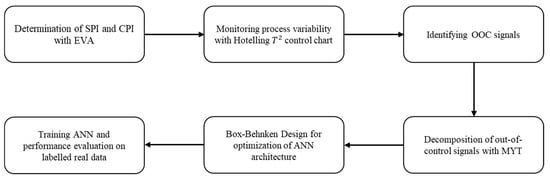
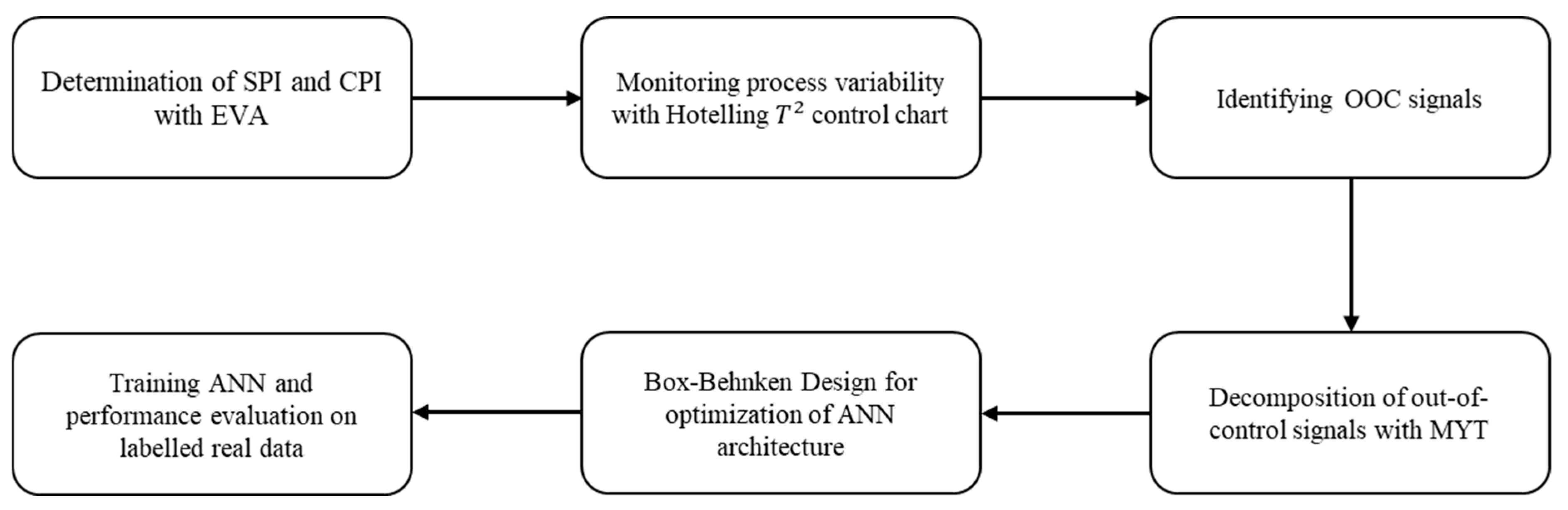
The proposed framework was implemented on a real-world manufacturing project to evaluate its effectiveness in detecting and classifying OOC signals. The overall workflow of the proposed framework, including EVA-based parameter extraction, Hotelling T² monitoring, MYT-based labeling, and ANN classification, is illustrated in Figure 1.

Figure 1. Application process flow chart.

The developed system enables simultaneous monitoring of project cost and schedule performance, early detection of OOC situations, and systematic classification of the variable(s) associated with these deviations. This structure supports managers in making proactive interventions and increases the effectiveness of project control and decision-making processes.

4.2. Data Collection and Processing

The study was conducted using real data from a manufacturing company. A nationally funded project was selected because it showed significant deviations from the planned cost and schedule despite its strategic importance for delivery within the planned cost and timeframe.

The project undertaken within the scope of the application consists of three main work packages and numerous sub-work packages: “Design and Concept Development,” “Validation and Prototype Production,” and “Production Verification and Improvement Studies.” The project was planned for 27 months, with a total cost of $54,489.26, and completed in 32 months for $91,383.54. Although the project consists of work packages and sub-work packages, the observations used in the ANN model were organized as CPI-SPI-based monitoring records rather than independent work packages. This project is fundamental for the company, and other project proposals that will proceed with a similar methodology are ongoing. Identifying the performance indicators associated with the deviations within this project and taking action will form the basis for similar project proposals. Furthermore, the intelligent system developed with this data will increase the company’s R&D efficiency by preemptively identifying potential deviations in new projects.

4.3. Determination of Parameters with EVA

The EVA method was applied to the selected project using information obtained from the company, and the calculations yielded CPI and SPI parameter values. Some examples of the calculations performed in the study are provided in Table 4. Parameter values below 1 indicate that the project fell short of its planned cost and/or duration. These CPI and SPI values were used as input variables in the subsequent multivariate analysis.

Table 4. Application of the EVA Method (for sample data).

Work Package	POC	PV ($)	EV ($)	AC ($)	CPI	SPI
**	83.33%	975.93	813.27	1171.11	0.69444	0.83333
**	83.33%	650.62	542.18	780.74	0.69444	0.83333
**	74.29%	2602.47	1933.27	3667.86	0.52708	0.74286
**	69.09%	3903.71	2697.11	8705.27	0.30982	0.69091
**	67.50%	3253.09	2195.84	5473.32	0.40119	0.67500
**	55.00%	65.06	35.78	97.59	0.36667	0.55000
**	66.00%	11,385.82	7514.64	13,604.42	0.55237	0.66000
**	59.88%	9108.65	5453.95	9829.21	0.55487	0.59877
**	80.00%	325.31	260.25	3488.94	0.07459	0.80000
**	46.75%	9759.27	4562.78	17,387.77	0.26241	0.46753

Note: Work package names are represented by “**” to preserve the confidentiality of the case company.

4.4. Monitoring Process Variability with Hotelling T² Control Chart

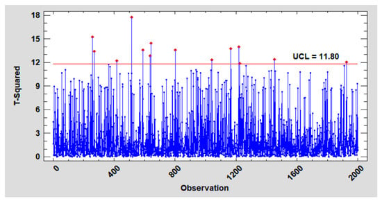
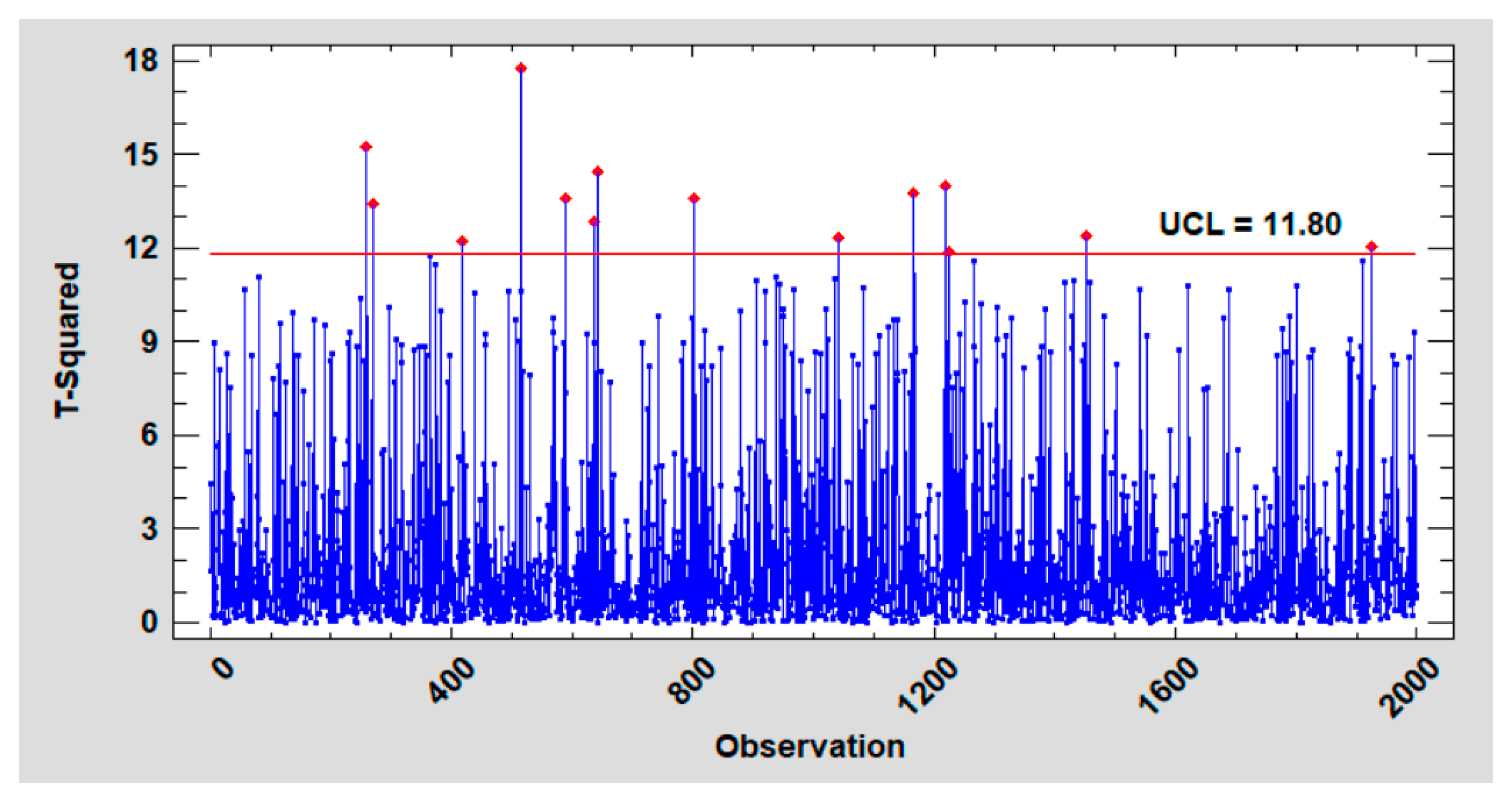
Before applying the Hotelling T² control chart, the underlying assumptions were checked. Since no violations of these assumptions were detected, the analysis proceeded. The Hotelling T² control chart for the case study data is given in Figure 2. In this case study, the number of monitored variables (CPI and SPI) was p = 2, and the significance level was selected as α = 0.0027. The upper control limit was calculated as UCL = 11.80 using the Hotelling T² control limit formulation given in Equation (2). Points outside the UCL indicate that the process is statistically out-of-control. These OOC observations were analyzed in more detail using the MYT decomposition method to identify the associated variable(s).

Figure 2. Hotelling T² chart. The red horizontal line indicates the UCL, and the red points indicate OOC observations.

4.5. Decomposition with MYT Method

The MYT method was used in the study to determine which parameter(s) were associated with the OOC situation. It was determined whether the OOC behavior was caused by the CPI, SPI or both parameters simultaneously. All OOC data required for training the ANN model were monitored and labeled accordingly.

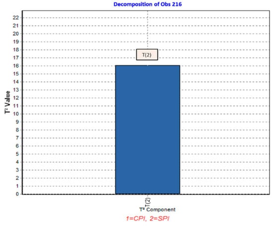
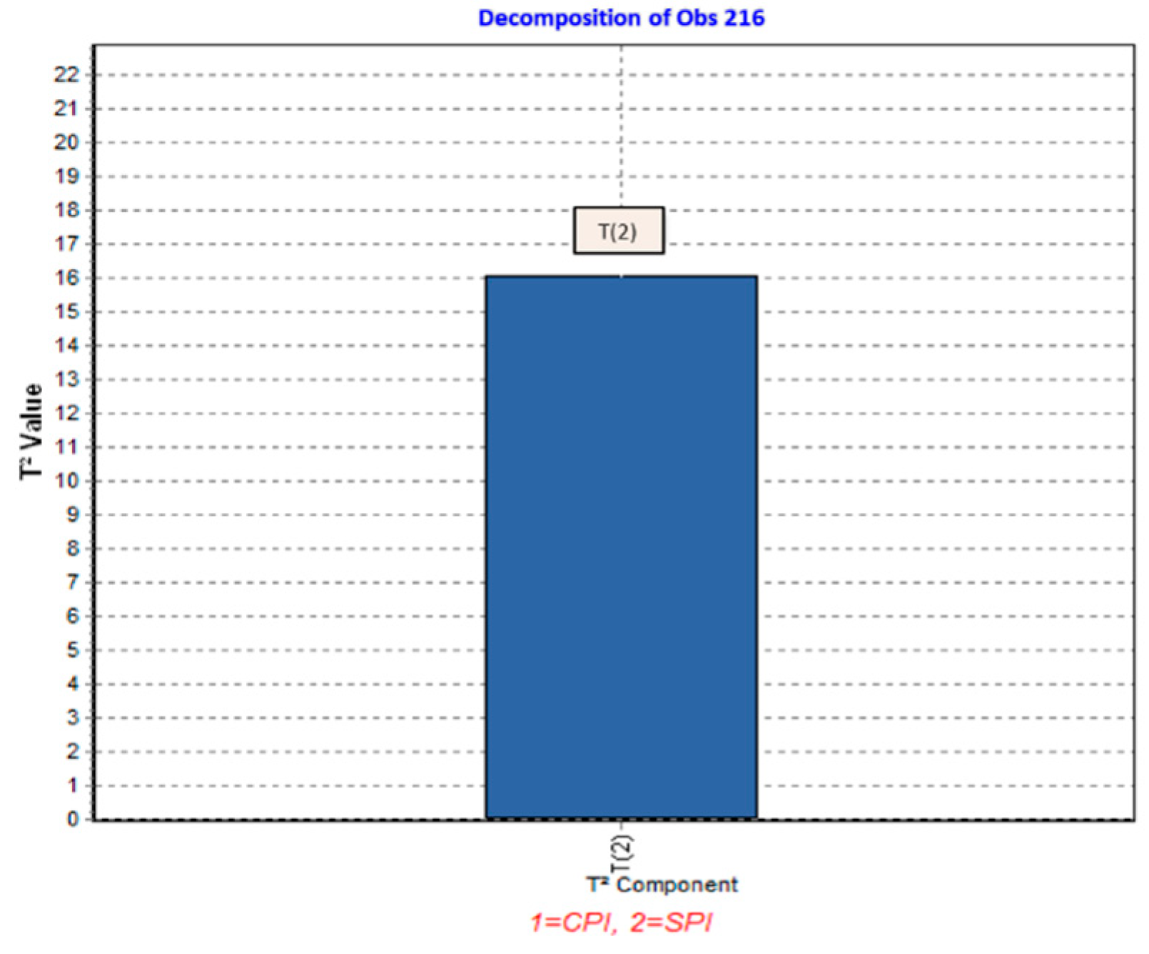
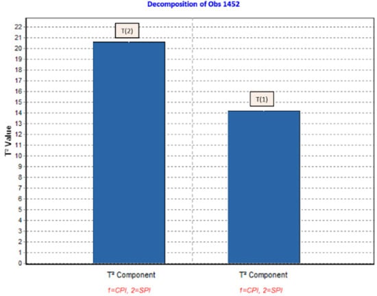
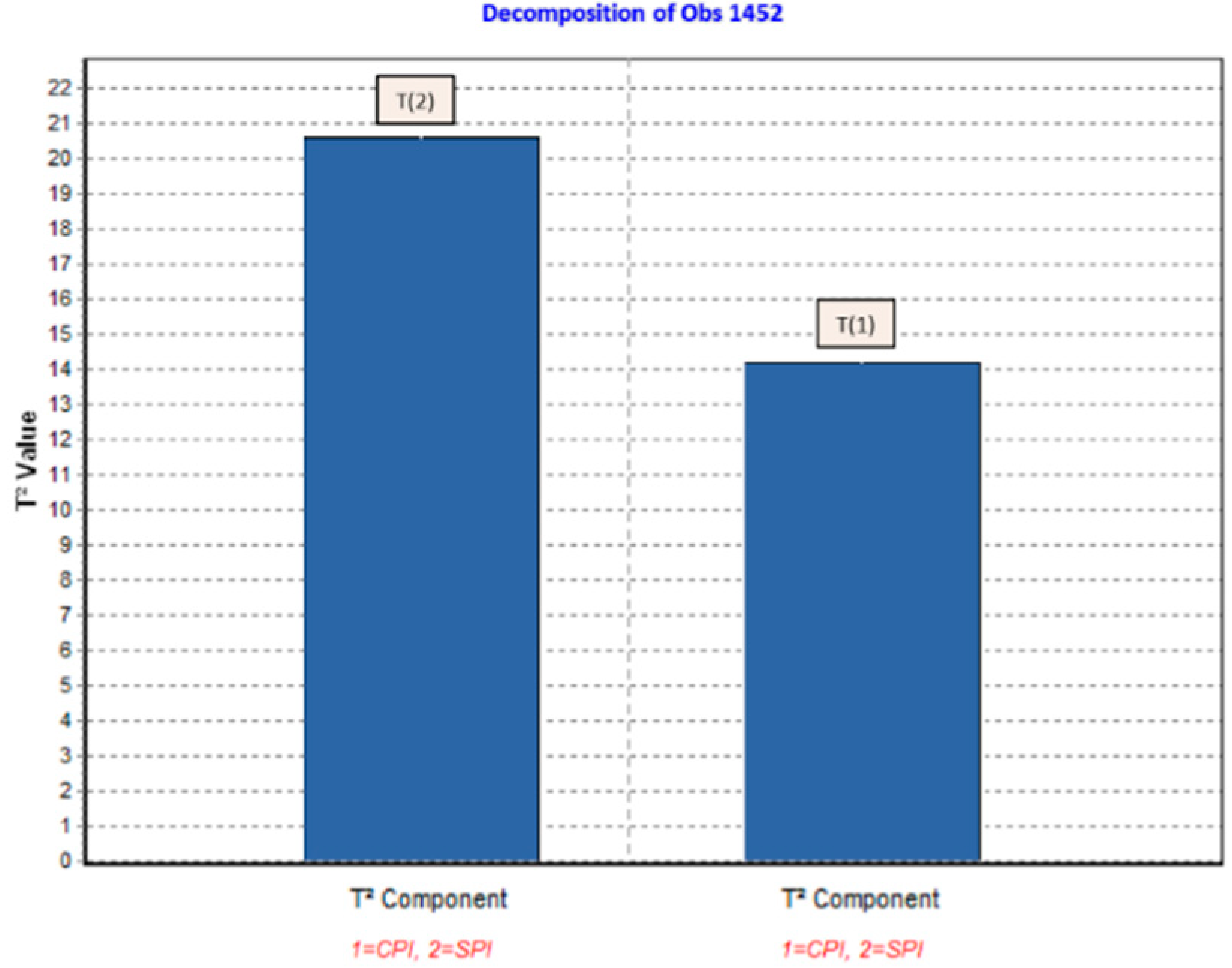
For illustrative purposes, randomly selected OOC points (216 and 1452) from the dataset were examined to determine the parameter associated with the OOC. The MYT decomposition results for these observations are presented in Figure 3 and Figure 4. Figure 3 shows that in observation 216, the OOC signal is associated with the second variable, the SPI parameter. In contrast, in observation 1452 in Figure 4, the OOC signal is jointly attributed to CPI and SPI. Labeled OOC observations derived from MYT decomposition were used to train the ANN model.

Figure 3. Sources of variability in observation 216.

Figure 4. Sources of variability in observation 1452.

4.6. Construction of the DOE-Supported ANN Architecture

In this study, an ANN model was developed to automatically classify OOC signals based on labels obtained from the Hotelling T² control chart and the MYT decomposition method. The Hotelling T² control chart was first used to detect OOC observations, and the MYT decomposition method was then applied to identify the variable(s) associated with each OOC signal.

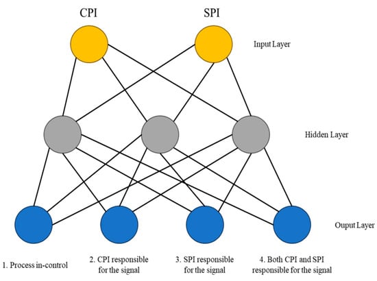
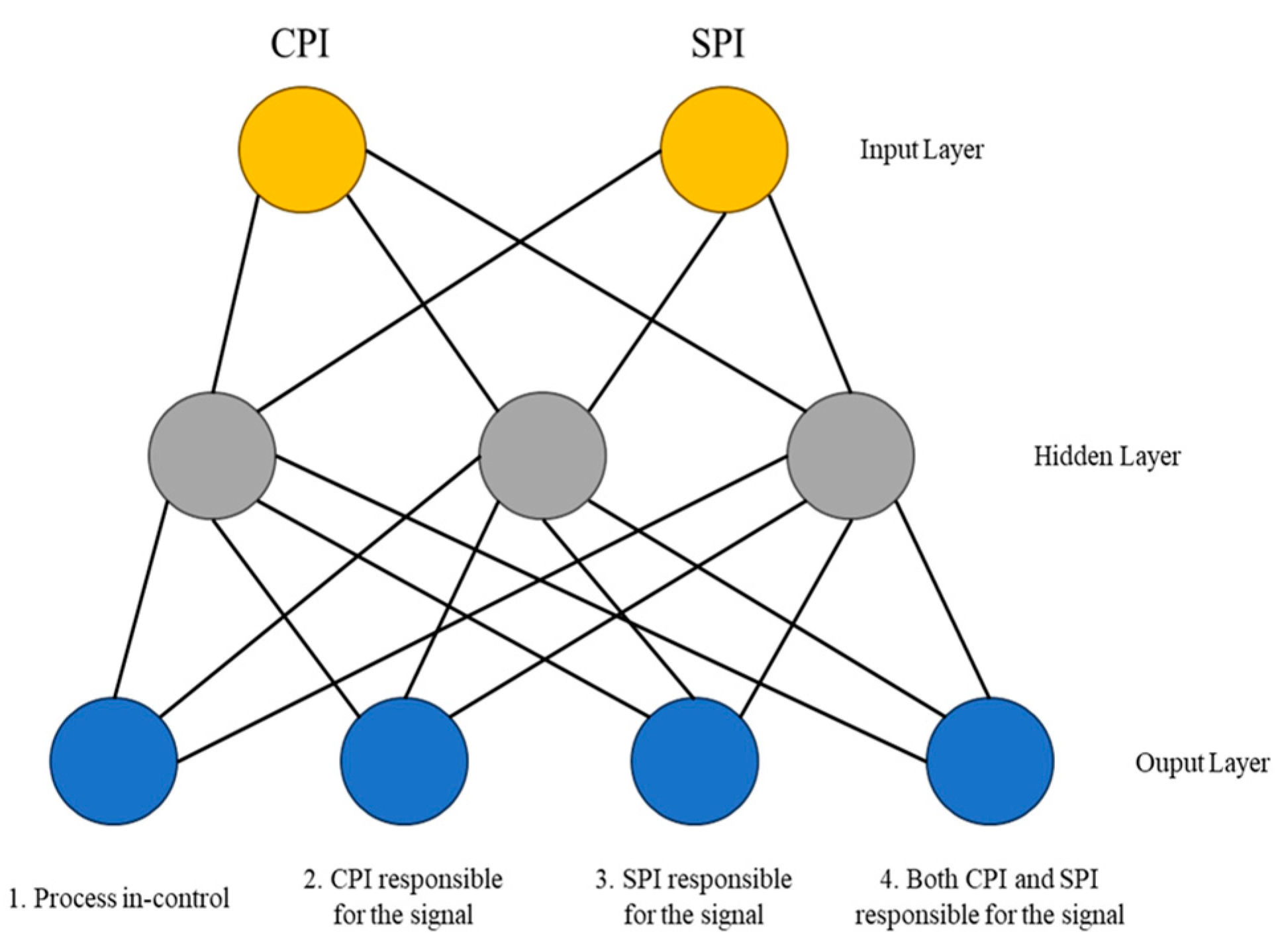
For ANN training and testing, the observations were labeled as 1 (process IC), 2 (CPI-related OOC), 3 (SPI-related OOC), and 4 (CPI-SPI-related OOC), as shown in Figure 5. The numerical labels assigned to the four classes were used solely as nominal/categorical identifiers. The MSE target was used only as a training error criterion, aiming for a value of 0. Final classification performance was evaluated using classification-based metrics such as accuracy, precision, recall, specificity, and F1-score.

Figure 5. ANN Model architecture.

To improve the accuracy of the designed ANN model and reduce the risk of overfitting, the dataset was split into 70% for training and 30% for testing. Accordingly, 1400 observations were used for training and 600 observations for testing. The ANN model was trained only on the training data, and the test data were used to evaluate generalization performance.

4.7. Experimental Design–Based ANN Architecture and Performance Evaluation of the Integrated System

Within the scope of the study, the Box–Behnken design was used as a hyperparameter optimization approach for the ANN models. Two learning algorithms were evaluated: Gradient Descent Backpropagation with Momentum and Adaptive Learning Rate, and the Levenberg–Marquardt algorithm. The response variable in the experimental design was the ANN training error criterion, and the objective was to determine the ANN hyperparameter combination that minimized the MSE. However, the final classification performance of the optimized ANN models was evaluated using classification-based metrics, including accuracy, precision, recall, specificity, and F1-score.

The design factors and levels for each learning method, determined based on expert opinions and the literature [55,56,57,58,59,60,61,62], are presented in Table 5. Optimum ANN settings were determined from the quadratic regression models generated by the experimental design, yielding the most suitable ANN architecture.

Table 5. Comparison of Box–Behnken experimental design results for ANN architecture.

	Number of Designs
	1	2
Learning Method	Gradient Descent Backpropagation Algorithm with Momentum and Adaptive Learning Rate	Levenberg–Marquardt Algorithm
Factors and Levels	x1: Learning Coefficient (0.005–0.05) x2: Momentum Coefficient (0.1–0.9) x3: Epoch Number (1–999) x4: Stopping Criterion (1.5–2) x5: Number of Hidden Neurons (10–80)	x1: Epoch Number (1–999) x2: Stopping Criterion (1.5–2) x3: Number of Hidden Neurons (10–80)
Number of Experiments	92	30
Regression Model	$\begin{array}{c}\widehat{y}=0.28185-0.09004x_2-0.73451x_3+\\ 0.77177x_3{x}_3-0.20541x_2{x}_3\end{array}$	$\begin{array}{c}\widehat{y}=0.48550-0.00209x_1+0.35566x_2-\\ 0.00988x_3+0.000001x_1{x}_1+0.00001x_1{x}_3\end{array}$
Coefficient of Determination	83.26%	85.14%
Optimum Factors and Levels	Momentum Coefficient: 0.72 Epoch Number: 793	Epoch Number: 915 Stopping Criterion: 1.5 Number of Hidden Neurons: 75

The experimental design results indicate that the ANN model trained using the Levenberg–Marquardt algorithm (Design 2) exhibits better performance compared to the alternative configuration, based on R². The higher coefficient of determination (85.14%) indicates improved model fit and error minimization capabilities under the proposed optimization framework.

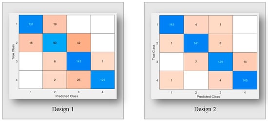
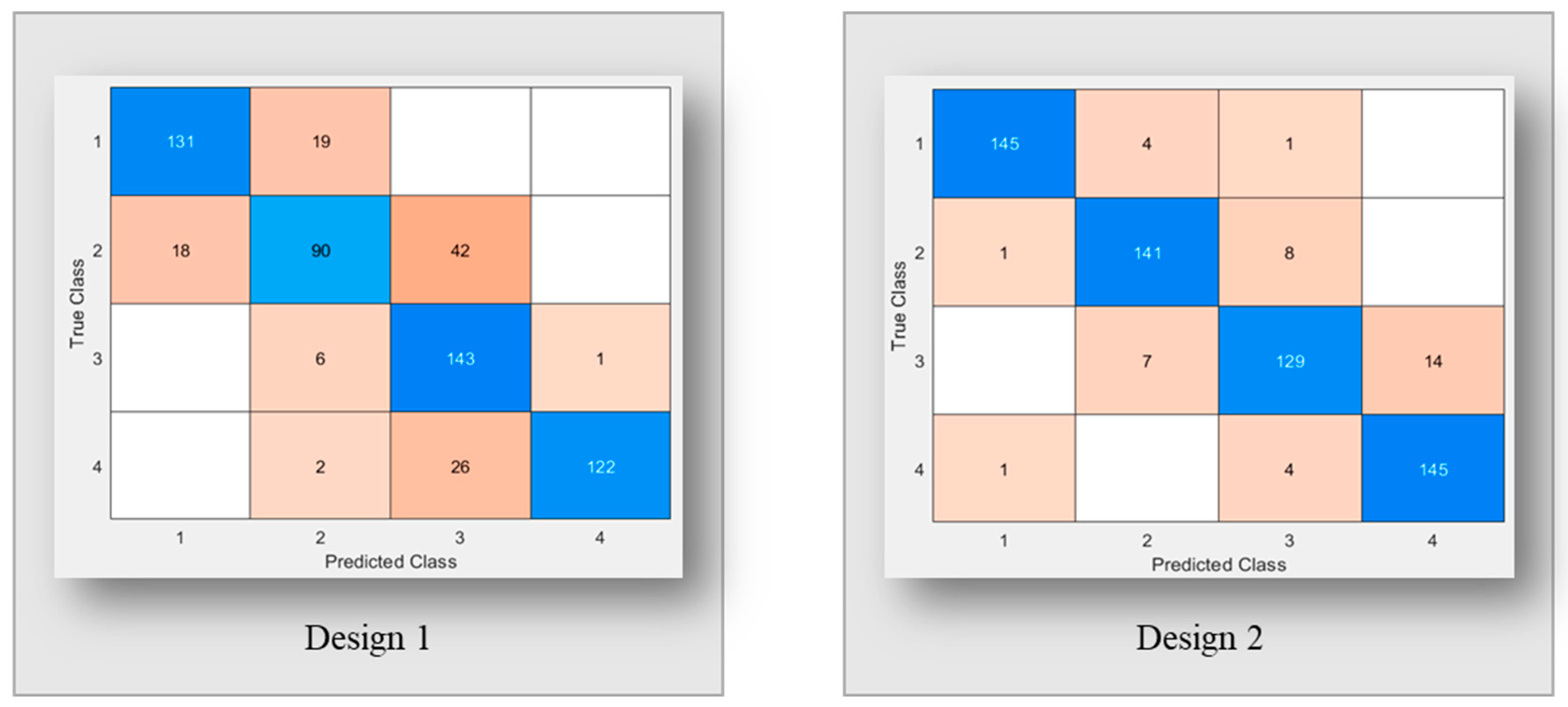
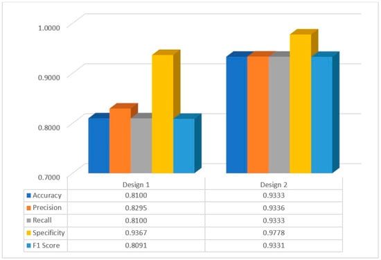
Within the scope of the study, a 4 × 4 confusion matrix for four classes (IC, CPI, SPI, and CPI-SPI) was generated to evaluate the performance of the ANN models on the test data, as presented in Figure 6. The performance metrics in Table 3 were calculated for each design based on the confusion matrix and presented in Figure 7.

Figure 6. Confusion matrix comparison.

Figure 7. Confusion matrix performance comparison.

In the four-class balanced dataset, Design 2 demonstrated better performance than Design 1 across all reported evaluation metrics. The confusion matrices show that Design 1 produced more misclassifications involving Class 3, whereas Design 2 exhibited a clearer diagonal pattern and better separation among classes. These results indicate that Design 2 provides better test performance and a lower error rate. The results confirm that the proposed framework can effectively classify OOC signals and distinguish whether they are associated with CPI, SPI, or both.

Overall, the results demonstrate that the proposed integrated framework is effective in detecting OOC situations and classifying the variable(s) associated with them. The integration of statistical process control, MYT-based signal interpretation, and optimized machine learning provides a decision-support tool for advanced process monitoring and continuous improvement.

5. Conclusions

Accurate interpretation of OOC signals is critical for maintaining stability and reliability in multivariate process monitoring systems. In this study, an integrated decision-support framework combining multivariate statistical process control and machine learning was developed.

The proposed approach combines the Hotelling T² control chart, the MYT decomposition method, and an ANN model optimized by using the Box–Behnken design. This framework enables monitoring of correlated process variables using performance metrics derived from EVA as multivariate inputs. The Hotelling T² chart was used to detect OOC signals, while the MYT decomposition method was used to identify the influencing variables. The outputs obtained from MYT were converted into labeled data and then used by the ANN model to classify the OOC signals according to the associated EVA-based performance indicator, namely CPI, SPI, or both.

The key contribution of this study is to transform statistical OOC decomposition into a machine-learning-based decision-support framework. Unlike traditional approaches, the proposed method not only detects OOC signals but also automatically classifies them using an optimized machine learning model. This approach provides a structured, actionable decision-support mechanism for identifying EVA-based performance indicators associated with process deviations.

The findings showed that the proposed framework achieves high classification performance and effectively distinguishes between different OOC scenarios. The integration of statistical monitoring, MYT-based signal interpretation, and optimized machine learning enhances the system’s interpretability and predictive capabilities.

Nevertheless, this study has several limitations. The proposed approach considered only the Hotelling T² control chart and ANN models, and the experimental design was limited to certain factors and levels. Since the application is based on a single manufacturing project, the findings should be interpreted as a case-based proof of concept rather than as evidence of universal generalizability. In addition, since the dataset consists of sequential project monitoring records, a random 70/30 train/test split may introduce the risk of data leakage due to the relationship between adjacent observations. Accordingly, future studies may use time-based data splitting or forward-chaining cross-validation approaches to evaluate model performance more comprehensively. Beyond this limitation, the framework could be extended by including alternative MCCs, such as MEWMA or MCUSUM; comparing different machine learning algorithms; applying alternative hyperparameter optimization methods; testing broader experimental settings; and validating the framework using additional project datasets. Furthermore, although the application focuses on a manufacturing project, the proposed framework can be adapted to other project-based sectors, such as construction, software development, and R&D, provided that reliable cost and schedule performance indicators are available.

References

- Montgomery, D.C. Introduction to Statistical Quality Control; John Wiley & Sons: Hoboken, NJ, USA, 2020. [Google Scholar]
- Imran, M.; Dai, H.-L.; Zaidi, F.S.; Hu, X.; Tran, K.P.; Sun, J. Analyzing out-of-control signals of T2 control chart for compositional data using artificial neural networks. Expert Syst. Appl. 2024, 238, 122165. [Google Scholar] [CrossRef] [Scilit]
- Midilli, Y.E. Utilizing Experimental Design to Optimize Parameters of Artificial Neural Networks: Example of Tobacco Industry. Master’s Thesis, Ondokuz Mayis University, Samsun, Turkey, 2018. [Google Scholar]
- Myers, R.H.; Montgomery, D.C.; Anderson-Cook, C.M. Response Surface Methodology: Process and Product Optimization Using Designed Experiments; John Wiley & Sons: Hoboken, NJ, USA, 2016. [Google Scholar]
- Hotelling, H. Multivariate quality control illustrated by the air testing of sample bombsights. In Techniques of Statistical Analysis; Eisenhart, C., Hastay, M.W., Wallis, W.A., Eds.; McGraw-Hill: New York, NY, USA, 1947; pp. 111–184. [Google Scholar]
- Asri, G.; Citra, F.; Nisa, S.; Lestari, T. The bread production process using application of the Hotelling T2 control chart. J. Phys. Conf. Ser. 2019, 1402, 022047. [Google Scholar] [CrossRef] [Scilit]
- Tomé, E.S.; Pimentel, M.; Figueiras, J. Damage detection under environmental and operational effects using cointegration analysis—Application to experimental data from a cable-stayed bridge. Mech. Syst. Signal Process. 2020, 135, 106386. [Google Scholar] [CrossRef] [Scilit]
- Zhao, Y.; He, X.; Zhang, J.; Ji, H.; Zhou, D.; Pecht, M.G. Detection of intermittent faults based on an optimally weighted moving average T2 control chart with stationary observations. Automatica 2021, 123, 109298. [Google Scholar] [CrossRef] [Scilit]
- Mashuri, M.; Ahsan, M.; Lee, M.H.; Prastyo, D.D.; Wibawati. PCA-based Hotelling’s T2 chart with fast minimum covariance determinant estimator and kernel density estimation for network intrusion detection. Comput. Ind. Eng. 2021, 158, 107447. [Google Scholar] [CrossRef] [Scilit]
- Wang, A.Q.; Pei, Y.; Qian, Z.; Zareipour, H.; Jing, B.; An, J.Y. A two-stage anomaly decomposition scheme based on multi-variable correlation extraction for wind turbine fault detection and identification. Appl. Energy 2022, 321, 119373. [Google Scholar] [CrossRef] [Scilit]
- Cacciarelli, D.; Kulahci, M. A novel fault detection and diagnosis approach based on orthogonal autoencoders. Comput. Chem. Eng. 2022, 163, 107853. [Google Scholar] [CrossRef] [Scilit]
- Ershadi, M.J.; Niaki, S.T.A.; Azizi, A.; Esfahani, A.A.; Abadi, R.E. Monitoring data quality using Hotelling T2 multivariate control chart. Commun. Stat. Simul. Comput. 2023, 52, 1591–1606. [Google Scholar] [CrossRef] [Scilit]
- Shojaee, M.; Noori, S.; Jafarian-Namin, S.; Johannssen, A. Integration of production-maintenance planning and monitoring simple linear profiles via Hotelling’s T2 control chart and particle swarm. Comput. Ind. Eng. 2024, 188, 109864. [Google Scholar] [CrossRef] [Scilit]
- Mahmood, T.; Ahmed, F.; Riaz, M.; Abbas, N. High-dimensional control charts with application to surveillance of grease damage in bearings of wind turbines. Prod. Manuf. Res. 2024, 12, 2377739. [Google Scholar] [CrossRef] [Scilit]
- Saha, S.; Khoo, M.B.C.; Chatterjee, K.; Godase, D.G. Multivariate triple sampling Hotelling’s T2 control chart. Qual. Technol. Quant. Manag. 2025, 23, 129–143. [Google Scholar] [CrossRef] [Scilit]
- Hsu, Y.C.; Wu, C.H. Application of Hotelling’s T2 control chart for non-destructive quality management of the green tea beverage rapid cooling process. J. Food Meas. Charact. 2025, 19, 5601–5610. [Google Scholar] [CrossRef] [Scilit]
- Mason, R.L.; Tracy, N.D.; Young, J.C. Decomposition of T2 for multivariate control chart interpretation. J. Qual. Technol. 1995, 27, 99–108. [Google Scholar] [CrossRef] [Scilit]
- Mason, R.L.; Chou, Y.M.; Young, J.C. Detection and interpretation of a multivariate signal using combined charts. Commun. Stat. Theory Methods 2011, 40, 942–957. [Google Scholar] [CrossRef] [Scilit]
- Mason, R.L.; Chou, Y.M.; Young, J.C. The relationship between the T2 statistic and the influence function. Commun. Stat. Theory Methods 2014, 43, 2844–2857. [Google Scholar] [CrossRef] [Scilit]
- Chen, Y.K.; Durango-Cohen, P.L. Development and field application of a multivariate statistical process control framework for health-monitoring of transportation infrastructure. Transp. Res. Part B Methodol. 2015, 81, 78–102. [Google Scholar] [CrossRef] [Scilit]
- Lee, S. Identification of the out-of-control variable based on Hotelling’s T2 statistic. Korean J. Appl. Stat. 2018, 31, 811–823. [Google Scholar] [CrossRef]
- Li, X.L.; Liu, S.S. Fault separation and detection algorithm based on Mason Young Tracy decomposition and Gaussian mixture models. Int. J. Intell. Comput. Cybern. 2020, 13, 81–101. [Google Scholar] [CrossRef] [Scilit]
- Sharifnia, S.G.; Saghaei, A. Exponential random graph modeling for diagnosis of out-of-control signals in social network surveillance: Signal interpretation in social networks with ERG modeling. Qual. Reliab. Eng. Int. 2021, 37, 1287–1306. [Google Scholar] [CrossRef] [Scilit]
- Hwarng, H.B.; Wang, Y. Shift detection and source identification in multivariate autocorrelated processes. Int. J. Prod. Res. 2010, 48, 835–859. [Google Scholar] [CrossRef] [Scilit]
- Rezki, N.; Kazar, O.; Mouss, L.H.; Kahloul, L.; Rezki, D. A hybrid approach for complex industrial process monitoring. J. Sci. Ind. Res. 2017, 76, 608–613. [Google Scholar]
- Awad, M.I.; AlHamaydeh, M.; Faris, A. Fault detection via nonlinear profile monitoring using artificial neural networks. Qual. Reliab. Eng. Int. 2018, 34, 1195–1210. [Google Scholar] [CrossRef] [Scilit]
- Ruelas-Santoyo, E.A.; Vargas-Rodríguez, B.L.; Cardiel-Ortega, J.J.; Llamas-Perez, G. Analysis of the Hotelling’s T2 multivariate control chart through fuzzy ARTMAP artificial neural network. DYNA 2018, 93, 21. [Google Scholar] [CrossRef] [Scilit] [PubMed]
- Tegegne, D.A.; Azene, D.K.; Atanaw, E.B. Design multivariate process statistical control procedure in the case of Ethio cement. Int. J. Qual. Reliab. Manag. 2022, 39, 1617–1636. [Google Scholar] [CrossRef] [Scilit]
- Kumar, A.; Das, A. A nonlinear process monitoring strategy with a 2-phase fault diagnosis approach. Eng. Res. Express 2022, 4, 025015. [Google Scholar] [CrossRef] [Scilit]
- Sabahno, H.; Amiri, A. New statistical and machine learning based control charts with variable parameters for monitoring generalized linear model profiles. Comput. Ind. Eng. 2023, 184, 109562. [Google Scholar] [CrossRef] [Scilit]
- Chen, B.S.; Huang, C.C.; Liao, T.W.; Kuo, C.F.J. Integration of the multivariate statistical control chart and machine learning to identify faults in the quality characteristics for polylactic acid with glass fiber composites in injection molding. Text. Res. J. 2024, 94, 2130–2146. [Google Scholar] [CrossRef] [Scilit]
- Okhrin, Y.; Schmid, W.; Semeniuk, I. A control chart for monitoring image processes based on convolutional neural networks. Stat. Neerl. 2025, 79, 12366. [Google Scholar] [CrossRef] [Scilit]
- Nourbakhsh, H.; Emam-Djomeh, Z.; Omid, M.; Mirsaeedghazi, H.; Moini, S. Prediction of red plum juice permeate flux during membrane processing with ANN optimized using RSM. Comput. Electron. Agric. 2014, 102, 1–9. [Google Scholar] [CrossRef] [Scilit]
- Pontes, F.J.; Amorim, G.F.; Balestrassi, P.P.; Paiva, A.P.; Ferreira, J.R. Design of experiments and focused grid search for neural network parameter optimization. Neurocomputing 2016, 186, 22–34. [Google Scholar] [CrossRef] [Scilit]
- Midilli, Y.E.; Elevli, S. Optimization of neural networks with response surface methodology: Prediction of cigarette pressure drop. In Proceedings of the 60th International Scientific Conference on Information Technology and Management Science of Riga Technical University (ITMS), Riga, Latvia, 10–11 October 2019; pp. 1–6. [Google Scholar] [CrossRef] [Scilit]
- Akbarzadeh, S.; Ahderom, S.; Alameh, K. A statistical approach to provide explainable convolutional neural network parameter optimization. Int. J. Comput. Intell. Syst. 2019, 12, 1635–1648. [Google Scholar] [CrossRef] [Scilit]
- Ibrahim, S.; Abdul Wahab, N. Improved artificial neural network training based on response surface methodology for membrane flux prediction. Membranes 2022, 12, 726. [Google Scholar] [CrossRef] [Scilit] [PubMed]
- Ibrahim, S.; Abdul Wahab, N. Optimizing neural network algorithms for submerged membrane bioreactor: A comparative study of OVAT and RSM hyperparameter optimization techniques. Water Sci. Technol. 2024, 89, 1701–1724. [Google Scholar] [CrossRef] [Scilit] [PubMed]
- Lipke, W.; Zwikael, O.; Henderson, K.; Anbari, F. Prediction of project outcome: The application of statistical methods to earned value management and earned schedule performance indexes. Int. J. Proj. Manag. 2009, 27, 400–407. [Google Scholar] [CrossRef] [Scilit]
- Zohoori, B.; Verbraeck, A.; Bagherpour, M.; Khakdaman, M. Monitoring production time and cost performance by combining earned value analysis and adaptive fuzzy control. Comput. Ind. Eng. 2019, 127, 805–821. [Google Scholar] [CrossRef] [Scilit]
- Mahmoudi, A.; Javed, S.A.; Deng, X. Earned duration management under uncertainty. Soft Comput. 2021, 25, 8921–8940. [Google Scholar] [CrossRef] [Scilit]
- Priyo, M. Earned value management system in Indonesian construction projects. Int. J. Integr. Eng. 2021, 13, 37–45. [Google Scholar] [CrossRef] [Scilit]
- Roghabadi, M.A.; Moselhi, O. Forecasting project duration using risk-based earned duration management. Int. J. Constr. Manag. 2022, 22, 3077–3087. [Google Scholar] [CrossRef] [Scilit]
- Konior, J. Determining cost and time performance indexes for diversified investment tasks. Buildings 2022, 12, 1198. [Google Scholar] [CrossRef] [Scilit]
- Zhang, X.; Zhang, X. An automated project carbon planning, monitoring and forecasting system integrating building information model and earned value method. J. Clean. Prod. 2023, 397, 136526. [Google Scholar] [CrossRef] [Scilit]
- Emblemsvåg, J. Lean project planning—Bridging last planner system and earned value management. Heliyon 2024, 10, e37810. [Google Scholar] [CrossRef] [Scilit] [PubMed]
- Ottaviani, F.M.; De Marco, A.; Narbaev, T.; Rebuglio, M.; Preziosa, S. A review and mapping of project schedule monitoring methods. Procedia Comput. Sci. 2025, 256, 1788–1795. [Google Scholar] [CrossRef] [Scilit]
- Hadian, H.; Rahimifard, A. Multivariate statistical control chart and process capability indices for simultaneous monitoring of project duration and cost. Comput. Ind. Eng. 2019, 130, 788–797. [Google Scholar] [CrossRef] [Scilit]
- Votto, R.; Ho, L.L.; Berssaneti, F. Multivariate control charts using earned value and earned duration management observations to monitor project performance. Comput. Ind. Eng. 2020, 148, 106691. [Google Scholar] [CrossRef] [Scilit]
- Elsaid, M.; Nassar, K.; Alqahtani, F.K.; Abotaleb, I. Comparative analysis of earned value management techniques in construction projects. Sci. Rep. 2025, 15, 23606. [Google Scholar] [CrossRef] [Scilit] [PubMed]
- Kocak, S. PRIMAVERA P6 Supported Cost Control with Earned Value Analysis in Construction Projects and an Application. Master’s Thesis, Akdeniz University, Antalya, Turkey, 2018. [Google Scholar]
- Mason, R.L.; Tracy, N.D.; Young, J.C. A practical approach for interpreting multivariate T2 control chart signals. J. Qual. Technol. 1997, 29, 396–406. [Google Scholar] [CrossRef] [Scilit]
- Montgomery, D.C.; Peck, E.A.; Vining, G.G. Introduction to Linear Regression Analysis; John Wiley & Sons: Hoboken, NJ, USA, 2021. [Google Scholar]
- Box, G.E.P.; Behnken, D.W. Some new three level designs for the study of quantitative variables. Technometrics 1960, 2, 455–475. [Google Scholar] [CrossRef]
- Lin, T.; Tseng, C. Optimum design for artificial neural networks: An example in a bicycle derailleur system. Eng. Appl. Artif. Intell. 2000, 13, 3–14. [Google Scholar] [CrossRef] [Scilit]
- Kim, Y.S.; Yum, B.J. Robust design of multilayer feedforward neural networks: An experimental approach. Eng. Appl. Artif. Intell. 2004, 17, 249–263. [Google Scholar] [CrossRef] [Scilit]
- Balestrassi, P.P.; Popova, E.; Paiva, A.P.; Marangon Lima, J.W. Design of experiments on neural network’s training for nonlinear time series forecasting. Neurocomputing 2009, 72, 1160–1178. [Google Scholar] [CrossRef] [Scilit]
- Laosiritaworn, W.; Chotchaithanakorn, N. Artificial neural networks parameters optimization with design of experiments: An application in ferromagnetic materials modeling. Chiang Mai J. Sci. 2009, 36, 83–91. [Google Scholar]
- Lasheras, F.S.; Vilán, J.V.; Nieto, P.G.; del Coz Díaz, J. The use of design of experiments to improve a neural network model in order to predict the thickness of the chromium layer in a hard chromium plating process. Math. Comput. Model. 2010, 52, 1169–1176. [Google Scholar] [CrossRef] [Scilit]
- Nazghelichi, T.; Aghbashlo, M.; Kianmehr, M.H. Optimization of an artificial neural network topology using coupled response surface methodology and genetic algorithm for fluidized bed drying. Comput. Electron. Agric. 2011, 75, 84–91. [Google Scholar] [CrossRef] [Scilit]
- Chen, M.Y.; Fan, M.H.; Chen, Y.L.; Wei, H.M. Design of experiments on neural network’s parameters optimization for time series forecasting in stock markets. Neural Netw. World 2013, 23, 369. [Google Scholar] [CrossRef] [Scilit]
- Midilli, Y.E.; Parsutins, S. Optimization of deep learning hyperparameters with experimental design in exchange rate prediction. In Proceedings of the 61st International Scientific Conference on Information Technology and Management Science of Riga Technical University (ITMS), Riga, Latvia, 15–16 October 2020; pp. 1–4. [Google Scholar] [CrossRef] [Scilit]
Disclaimer/Publisher’s Note: The statements, opinions and data contained in all publications are solely those of the individual author(s) and contributor(s) and not of MDPI and/or the editor(s). MDPI and/or the editor(s) disclaim responsibility for any injury to people or property resulting from any ideas, methods, instructions or products referred to in the content. |
© 2026 by the authors. Licensee MDPI, Basel, Switzerland. This article is an open access article distributed under the terms and conditions of the Creative Commons Attribution (CC BY) license.