Probabilistic Assessment of Transit Heavy-Vehicle Impacts on CO₂e Emissions and External Pollution Costs in Urban Transport Corridors

Abstract

Heavy-duty transit vehicles (N1–N3) (heavy vehicles) can generate disproportionate environmental and economic impacts in urban transport corridors despite representing a relatively small share of total traffic volume. This study develops an integrated probabilistic framework for assessing the relationships between traffic-flow variability, CO₂e emissions, particulate-matter-derived climate impacts, and external pollution costs associated with transit transport. The methodology combines traffic-flow modeling, emission estimation, PM-to-CO₂e transformation, probabilistic analysis, Monte Carlo simulation, sensitivity analysis, and scenario-based intervention assessment. Separate analyses were conducted for M1 passenger vehicles and heavy vehicles to evaluate differences in emission behavior, uncertainty, and economic impacts. The results indicate substantial structural differences between light-duty and heavy-vehicle regimes. Passenger-car traffic exhibited relatively stable emission distributions, whereas heavy vehicles demonstrated significantly greater variability, uncertainty, and emission intensity. Sensitivity analysis identified heavy-vehicle flow as the dominant factor influencing overall system emissions and pollution costs. Scenario analysis indicated that restrictions targeting heavy-vehicle traffic have the potential to generate considerably larger environmental benefits than generalized traffic-reduction measures. Probabilistic assessment further revealed that heavy vehicles contribute disproportionately to high-emission risk regimes and uncertainty propagation within the system. The proposed framework provides an integrated approach for evaluating climate impacts, uncertainty and economic externalities of transit transport. The results highlight the importance of heavy-vehicle management in reducing emissions and pollution costs while supporting risk-informed transport policy development.

1. Introduction

Transit transport in urban and regional traffic networks has a disproportionate impact on both air quality and infrastructure load [1,2]. The literature consistently highlights that heavy vehicles, although they account for a relatively small share of traffic flows, generate a significant share of emissions and external costs. For example, in the Paris region, urban freight transport is found to account for only 6% of trips and 8% of the distance traveled but generates 36% of the total social costs of air pollution caused by road transport [3]. This indicates a structural disproportion between the share of flow and the environmental impact.

Similarly, a regional-scale analysis in Ontario showed that medium and heavy vehicles cause approximately $1.9 billion in annual transboundary damage costs, equivalent to $0.16 per kilometer traveled [4]. These results confirm that the impact of heavy vehicles is not limited to local pollution but has a wider interregional effect.

At the urban level, empirical evaluation in Hong Kong has shown that freight and bus traffic are strongly correlated with NOx emissions, and their intensity increases significantly on weekdays due to increased transport demand [5]. Meanwhile, passenger cars, although dominating the traffic structure, generate a relatively lower contribution of NOx and particulate matter per kilometer, but remain the main source of CO and volatile organic compounds [6].

In addition, validation studies of emission models have revealed that macro models can significantly underestimate NOx emissions from heavy vehicles. Comparing the results of the MATSim–HBEFA model with real PEMS measurement values, it was found that on certain road sections, NOx from heavy vehicles can be underestimated by up to 100 times [7]. This is of fundamental importance in assessing the role of transit transport in the city’s emission balance.

The formation of transport emissions is directly related to the type of vehicle, speed profile, load, and traffic regime [8]. The literature emphasizes that the use of average speed alone for emission assessment is methodologically limited, since real emissions strongly depend on instantaneous speed and acceleration [9]. Microscopic models allow us to capture the second-by-second dynamics of emissions but require detailed input data and more complex calibration.

Experimental PEMS measurements have shown that real NOx emissions can be about 50% higher than previously used laboratory estimates [10]. This is especially relevant for heavy vehicles with advanced systems for treating exhaust gases, the effectiveness of which depends on real operating conditions.

The speed profile and road gradient are also of fundamental importance. In modeling CO₂ emissions from CNG and diesel trucks, it has been found that excluding the road profile can lead to an underestimation of emissions by up to 24% [11]. This confirms that estimating emissions without topographic parameters can distort results, especially in hilly areas.

The analysis of urban intersections also reveals the importance of traffic regimes. Studies indicate that saturated conditions, characterized by braking–acceleration cycles, amplify the differences in emissions between signalized intersections and roundabouts [12]. Under unsaturated conditions, the differences in emissions between intersection types become less significant, and the results of the methods often diverge.

A study in alpine regions showed that a nighttime ban on >7.5 t vehicles had a limited impact on annual concentrations and, in some areas, even led to an increase in concentrations during the morning peak due to traffic congestion [13]. This confirms that time restrictions can have a temporal redistribution effect on emissions.

Spatial restrictions include low emission zones (LEZs), city center restrictions or transit diversions. In the case of Milan, high-resolution bottom-up emission modeling found that emissions were lower in the LEZ area due to a cleaner fleet and lower traffic volumes [14]. This suggests that spatial measures can have a locally tangible effect.

Vehicle class restrictions include weight limits, filtering of emission standards, or age restrictions. In Hebei Province, simulations of emission reduction scenarios showed that updating emission standards could reduce VOC emissions by up to 80% [15]. This shows the potential of technological restrictions.

A study conducted in Maribor (Slovenia) showed that eliminating the top 10% of black carbon (BC) emitters would reduce emissions by up to 39%, while removing vehicles older than 15 years would reduce emissions by approximately 19% [16]. This confirms that selective class restrictions can be more effective than general restrictions.

It should be noted that the environmental performance of heavy vehicles is not uniform across the fleet. Emission characteristics vary substantially according to propulsion technology, emission-control systems, vehicle age, fuel type, load factor, and operational practices. Modern Euro VI diesel vehicles equipped with advanced SCR and particulate-filter technologies, as well as battery-electric, hydrogen fuel-cell, and alternative-fuel heavy vehicles, may exhibit significantly lower pollutant emissions than older conventional fleets. Consequently, the environmental impact of heavy vehicles depends not only on the vehicle category but also on fleet composition and operational characteristics.

The impact of transit restrictions on air pollution has been assessed in the literature using before–after, difference-in-differences, and modeling approaches. However, empirical results show that the effect is often heterogeneous and dependent on meteorological conditions and traffic redistribution.

Analysis of port accesses using GPS data showed that emission “hot spots” form at entrances and highway junctions, and emission intensity is strongly affected by low-speed modes [17]. This means that even if the total volume of traffic decreases, local congestion nodes can remain high-pollution hotspots.

The impact of transit transport restrictions on traffic capacity and travel times is twofold: in the short term, congestion reduction is often observed on restricted sections, but at the system level, the effects of flow redistribution and the formation of new bottlenecks may become apparent.

Comparison of macroscopic and microscopic modeling shows that aggregated average speed models do not always adequately reflect the impact of congestion on emissions and travel time [18,19]. Therefore, when assessing the impact of restrictions, it is necessary to consider driving dynamics.

The assessment of transit-transport emissions and their interaction in the literature is based on modeling methods of varying levels of detail—from macroscopic traffic models to microsimulation and integrated emissions–air quality chains. The choice of method directly determines the accuracy and interpretation of the results.

Transport-emission modeling is commonly divided into macroscopic and microscopic approaches. Macroscopic models describe traffic conditions using aggregated variables such as average traffic speed, traffic-flow volume, vehicle-kilometers traveled (VKT) and network-level travel demand. These models evaluate the collective behavior of traffic streams and are typically applied at corridor, urban, or regional scales. In contrast, microscopic models simulate the movement of individual vehicles and explicitly represent vehicle-specific characteristics, acceleration–deceleration behavior, lane-changing actions, and car-following dynamics. Because emissions are strongly influenced by instantaneous operating conditions, microscopic approaches generally provide a more detailed representation of emission-generation processes, although at the cost of substantially greater data and computational requirements.

Macroscopic models are therefore particularly suitable for large-scale strategic assessments, whereas microscopic models are more appropriate when detailed traffic dynamics and vehicle-level emission processes must be represented [20]. This approach is suitable for spatial planning but has limited representation of driving dynamics.

Microsimulation models (e.g., VISSIM integration with emission models) allow the estimation of instantaneous speed and acceleration profiles. The integrated VISSIM–CMEM platform in Beijing has shown that emissions strongly depend on instantaneous acceleration and the driving mode [21]. This is particularly important for intersection and congestion analysis.

A comparison of intersection controls (roundabout vs. signalized) using microsimulation has shown that roundabouts often generate lower NOx and PM emissions, although the differences in emissions are smaller than in operational efficiency [22].

A two-level optimization model under disruption conditions has shown that signal optimization reduces both travel time and emissions, but the computational cost is very high [23]. This highlights the computational complexity of micromodels.

Recent studies have increasingly applied dynamic traffic-simulation environments such as VISSIM and Aimsun to analyze urban corridors, signalized intersections, and multimodal transport networks. These platforms enable detailed representation of vehicle interactions, queue formation, stop-and-go dynamics, acceleration profiles, and corridor-level operational performance. Because trajectory-level information can be directly linked to emission-estimation modules, dynamic simulation approaches are particularly useful for evaluating the environmental consequences of traffic-management strategies, signal-control modifications, and corridor reconfiguration measures. However, despite their high behavioral realism, such models generally require extensive calibration data, substantial computational resources, and site-specific network information, which may limit their applicability for broader probabilistic policy assessment and uncertainty analysis.

In contrast, the framework proposed in the present study focuses on system-level uncertainty characterization, probabilistic risk assessment, and climate-impact evaluation. Rather than reproducing detailed vehicle trajectories within a specific corridor, the approach is intended to evaluate the sensitivity, variability, and economic implications of different transport-emission regimes under uncertainty. Consequently, the framework should be viewed as complementary to dynamic simulation methodologies rather than as a replacement for them.

Previous studies have indicated that transport-emission estimates may vary considerably depending on the model structure, input data, and calibration assumptions, highlighting the importance of uncertainty assessment in transport-emission research [24]. This indicates methodological uncertainty.

The need for updates to the MOVES model was highlighted in an analysis of US commercial transport, where it was found that emissions results strongly depend on the actual fleet structure [25]. This confirms that emission models need to be calibrated with local data.

A review of integrated models has shown that there is no “best” single model combination, and the choice depends on the purpose of the study, scale, and data availability [26]. Emissions are identified as the most uncertain component of air quality modeling.

Integrated agent modeling (MATSim) in combination with emissions and dispersion models allows tracing the entire causal chain from transport demand to population exposure [27]. Such models allow for the assessment of policy scenarios at the microscale.

Integrated modeling in Ontario has shown that a 5% share of zero-emission trucks can reduce GHG emissions by 0.8 MtCO₂ and generate cross-border air quality co-benefits of $83/tCO₂ [4]. This suggests that climate policy measures can have significant local air quality effects.

Multimodal dynamic analysis has shown that route selection based on total cost, emission cost, and exposure cost leads to a balanced outcome, reducing both travel time and emissions [28]. However, emission and exposure criteria emphasize different aspects of the system and cannot be considered separately.

Research in the UK has shown that rapid deployment of BEVs can significantly reduce CO₂ and NOx emissions and generate monetary benefits of up to £1.3 billion, but too slow a transition creates risks of infrastructure and energy system strain [29]. This illustrates the importance of the time dimension of technological transformation.

A two-level game model analysis of mobility service providers (MSPs) shows that stricter carbon policy standards reduce emissions but can increase mobility prices and reduce consumer surplus [30]. Thus, regulatory measures have a direct distributional effect.

Despite the extensive literature on transit emissions and the impact of restrictions, significant gaps remain in research, including the transferability of results, the assessment of heavy-duty and light-duty interactions, and the lack of integrated optimization models.

Many studies analyze heavy and light transport separately but rarely model the dynamic interaction between them. A study comparing MATSim and PEMS showed that the NOx contribution of heavy transport can be up to 100 times higher than that of light vehicles, but macro models often underestimate this disproportion [31,32]. This emphasizes the necessity to model the interaction between different classes in more detail at the network level.

The Hebei Province (China) emissions inventory showed that non-local trucks account for a significant proportion of total emissions [10]. This emphasizes the necessity for systematic, cross-category models.

Although models exist that integrate emissions and travel time [33], such models have not yet been widely applied to the optimization of transit restrictions. Most policy evaluations analyze emissions or capacity separately.

The carbon policy model for mobility service providers also analyzes the trade-off between emissions and prices but does not include detailed network traffic optimization [34]. This indicates that large-scale, multi-level optimization models that integrate transport demand, emissions, health effects, and economic costs are still lacking.

Many studies highlight the lack of local emission factors and real-world speed profiles. Validation of emission models in Hong Kong has shown that modeled values can differ by up to 50% from real-world measurements [35]. This confirms the need to develop local emission databases.

Despite the extensive body of literature addressing transit-transport emissions, heavy-vehicle restrictions, and urban air-pollution mitigation strategies, several important methodological and systemic gaps remain unresolved. Existing studies are frequently based on localized case studies whose results are strongly context-dependent and difficult to generalize across different urban transport corridors. Furthermore, most previous research evaluates either emissions, traffic-flow performance, or economic impacts separately, while integrated probabilistic frameworks combining traffic-flow variability, CO₂e formation, particulate-matter-derived climate effects, and external economic costs remain limited. Current approaches also tend to analyze heavy-duty and passenger-car transport independently, without systematically modeling their interaction within the same transport system.

Another important limitation concerns the deterministic nature of many transport-emission assessments. Conventional macroscopic approaches often rely on average-speed assumptions and aggregated emission factors, which may substantially underestimate the variability and uncertainty of heavy-vehicle emissions under real operational conditions. Although several studies have applied Monte Carlo simulations, sensitivity analysis, or traffic microsimulation separately, relatively few investigations integrate probabilistic uncertainty analysis, exceedance-risk evaluation, marginal-benefit assessment, and external pollution-cost modeling into a single systems-level framework focused specifically on heavy vehicles in urbanized corridors. Consequently, there remains a lack of comprehensive methodologies capable of simultaneously evaluating climate impact, emission uncertainty, operational sensitivity, and economic externalities associated with heavy-vehicle flows.

The scientific novelty of this study lies in the development of an integrated probabilistic framework for assessing the climate and economic impacts of transit heavy vehicles in urbanized transport corridors. Unlike conventional deterministic transport-emission studies, the proposed methodology combines traffic-flow modeling, PM → CO₂e transformation, probabilistic emission analysis, Monte Carlo uncertainty assessment, Pearson correlation analysis, sensitivity analysis, exceedance-probability evaluation, and marginal-benefit modeling within a unified analytical structure.

Importantly, the contribution of the present study does not reside in the introduction of a new standalone statistical technique. Monte Carlo simulation, sensitivity analysis, probabilistic risk assessment, and scenario modeling are well-established methods individually. The novelty lies in their integration into a unified transport-emission–economic assessment framework specifically designed for heavy-vehicle corridors. To the best of the authors’ knowledge, few previous studies have combined traffic-flow variability, PM-derived climate-equivalent impacts, exceedance-risk assessment, marginal benefit analysis, and external pollution-cost evaluation within a single probabilistic decision-support structure. Consequently, the proposed framework advances methodological integration rather than introducing a new mathematical algorithm.

A further novel contribution of the study is the separate yet interconnected analysis of M1 passenger-car flows and heavy vehicles, allowing the identification of strong structural disproportions between traffic intensity, emission formation, and external economic costs. The results demonstrate that heavy vehicles act not only as the dominant source of CO₂e emissions but also as the primary generator of stochastic uncertainty, high-emission regimes, and external financial damage within the transport system.

In addition, the study introduces an exceedance-probability and marginal-benefit interpretation of transit transport interventions, enabling transport policies to be evaluated not only from the perspective of average emissions reduction but also in terms of climate-risk mitigation, uncertainty reduction, and diminishing-return dynamics. This system-level integration of probabilistic risk analysis, climate-impact assessment, and economic externality evaluation provides a substantially more comprehensive methodological approach than traditional aggregated transport-emission models and contributes to the advancement of climate-oriented transport-policy optimization methodologies.

2. Materials and Methods

This section describes the methodological framework used to assess the environmental and economic impacts of transit heavy vehicles in an urbanized transport corridor. The section first presents the general modeling structure and analytical workflow, followed by the procedures used for traffic-flow data generation, emissions estimation, PM-to-CO₂e transformation, financial-cost assessment, and probabilistic scenario analysis. The purpose of this section is to provide a transparent explanation of how traffic-flow variability was transformed into climate-impact indicators and external pollution costs within a unified probabilistic framework.

2.1. Research Structure and General Modeling Scheme

This study uses an integrated modeling approach of transport flows, emissions, climate impacts, and economic costs to assess the impact of transit transport on an urbanized transport corridor. The methodology is based on the principle of multi-level analysis, combining traffic-flow analysis, emissions calculation, CO₂ equivalent transformation, statistical analysis, scenario modeling and economic impact assessment.

The 60%, 65% and 70% heavy-vehicle restriction scenarios were intentionally selected as exploratory high-intervention cases designed to investigate the upper sensitivity limits of the transport emissions system. These scenarios should not be interpreted as direct policy recommendations or predictions of immediately achievable traffic reductions. Instead, they represent stress-test conditions intended to evaluate the potential environmental response of the system under progressively restrictive heavy-vehicle management assumptions.

The general modeling chain in this study consists of four main stages:

• Analysis of transport flows;
• Modeling of emissions and PM → CO₂e transformation;
• Assessment of the financial impact of pollution;
• Statistical and probabilistic scenario assessment.

The logic of the study is based on the causal chain of emissions formation:

$$Q\to E_{{\mathrm{C}\mathrm{O}}_2}+E_{PM}\to {CO}_{2e}\to C_f$$

(1)

where Ԛ—transport flow; $E_{{\mathrm{C}\mathrm{O}}_2}$—direct CO₂ emissions; $E_{PM}$—particulate matter emissions; ${CO}_{2e}$—total climate impact equivalent; $C_f$—financial cost of pollution.

The study separately modeled two main transport categories:

• M1-class passenger cars;
• N1–N3-class heavy transit transport.

This division was chosen due to fundamentally different emission generation modes, energy efficiency, and disproportionate impact of heavy vehicles on climate and air quality systems.

The analytical workflow was designed to progressively transform traffic-flow information into environmental and economic impact indicators. Traffic-flow distributions were first generated and statistically characterized. These flow values were subsequently converted into emission estimates using emission-factor-based calculations. The resulting CO₂ and particulate matter emissions were then transformed into integrated climate-impact indicators expressed as CO₂ equivalents. Finally, probabilistic, sensitivity, and scenario analyses were applied to evaluate uncertainty propagation, intervention effectiveness, and associated economic externalities.

2.2. Processing of Transport-Flow Data

The study used synthetic transport-flow data generated based on empirical flow amplitudes and probability distributions. The use of synthetic traffic-flow data was motivated by the methodological objective of evaluating uncertainty propagation and probabilistic system behavior across a wide range of operating conditions. The generated flow ranges were not selected arbitrarily but were constrained by traffic-volume intervals reported in previous studies of urban arterial corridors and heavy-vehicle routes. Synthetic data generation enabled systematic exploration of both typical and extreme traffic states that are often underrepresented in short-term field measurements.

The study does not represent a specific measured transport corridor. Instead, it considers a generalized urbanized transport corridor designed to reflect traffic conditions commonly reported in the literature for mixed passenger-car and transit-heavy traffic environments. The empirical flow amplitudes used for synthetic-data generation were derived from traffic-volume ranges reported in previous transport and freight-corridor studies cited in the Introduction Section 1.

For the M1 category, traffic flows were represented within an interval of approximately 1800–2800 vehicles h⁻¹, corresponding to moderate-to-high urban corridor demand conditions. For the N1–N3 category, flows were represented within an interval of approximately 50–300 vehicles h⁻¹, reflecting typical heavy-vehicle activity levels reported for transit-oriented corridors. Synthetic observations were generated using probability distributions constrained by these empirical ranges in order to reproduce plausible operating conditions rather than exact site-specific measurements.

Such an approach is widely applied in probabilistic transport and environmental modeling when the objective is to investigate system sensitivity, uncertainty structure and scenario responses rather than reproduce a specific corridor at a specific time. The generated datasets therefore represent plausible traffic regimes observed in urban transport systems rather than exact measurements from a single location. For the M1 transport segment, the following was formed: $n_{M1}=300$. Sample of simulated cases: $n_{N1–N3}=1350$.

Transport flows are defined as:

$$Q_i\in [Q_{min},Q_{max}]$$

(2)

where $Q_i$—individual simulated flow case; $Q_{min},Q_{max}$—minimum and maximum empirical flow limits.

For the M1 segment, $Q_{M1}\in [1719,2770]$ veh h⁻¹; and for the N1–N3 segment, $Q_{N1–N3}\in [53,293]$ veh h⁻¹.

The following methods were used in the analysis of the flow distribution:

• Histograms;
• Kernel density functions (KDFs);
• Empirical 95% intervals;
• Quartile analysis of variance.

The empirical distribution was estimated using:

$$f_h(x)={\displaystyle \frac{1}{nh}}{\sum }_{i=1}^{n}K({\displaystyle \frac{x-x_i}{h}})$$

(3)

where K—kernel function; h—smoothing parameter; $x_i$—individual observations.

The sample sizes were selected to provide sufficient representation of distributional variability while maintaining computational efficiency for probabilistic analysis. The larger N1–N3 sample was intentionally used to capture the greater heterogeneity and multimodal behavior observed in heavy-vehicle traffic regimes. Preliminary testing indicated that additional increases in sample size produced only marginal changes in the estimated distributional statistics and uncertainty intervals.

2.3. Emissions Modeling Methodology

Direct CO₂ emissions were calculated using the emission factor method:

$$E_{{\mathrm{C}\mathrm{O}}_2}=Q·{EF}_{{\mathrm{C}\mathrm{O}}_2}·L$$

(4)

where $E_{{\mathrm{C}\mathrm{O}}_2}$—CO₂ emissions (kg); Q—transport flow; ${EF}_{{\mathrm{C}\mathrm{O}}_2}$—emission factor; L—length of the road under consideration (km).

Calculation of particulate emissions is done analogously:

$$E_{PM}=Q·{EF}_{PM}·L$$

(5)

where ${EF}_{PM}$—particulate matter emission factor.

Since heavy-vehicle emissions strongly depend on operating modes, emission factors were interpreted as stochastic quantities: $EF~\mathrm{{\rm N}}(\mu ,\sigma )$ allowing for modeling of regime uncertainty.

To represent operational variability, emission factors were treated as stochastic parameters. Probability distributions were assigned based on reported variability ranges from the literature, and random sampling was performed within these bounds during Monte Carlo simulation. This approach enabled the representation of uncertainty associated with vehicle operating conditions, fleet heterogeneity, and traffic regimes.

PM-to-CO₂e Transformation Method

The impact of particulate matter on the climate system was transformed into CO₂ equivalent using the conversion factor:

$${CO}_{2e,PM}=E_{PM}·\alpha$$

(6)

where ${CO}_{2e,PM}$—CO₂ equivalent of PM origin; $\alpha$—PM $\to {CO}_{2e}$ transformation coefficient.

The total climate impact is calculated as:

$${CO}_{2e,total}=E_{{\mathrm{C}\mathrm{O}}_2}+{CO}_{2e,PM}$$

(7)

This methodology allows for the integration of both the direct impact of combustion and the indirect impact of aerosols into the overall climate indicator.

To improve methodological transparency and reproducibility,

Table 1. Principal model parameters adopted in the probabilistic framework.

Parameter	Symbol	Unit	Value	Assumption/Description
Number of synthetic observations per traffic segment	n	–	150	Synthetic sample generation for each traffic segment
Corridor length	L	km	4	Urbanized transport corridor segment
Heavy-duty vehicle PM emission factor	EFPM, HGV	g km−1 veh−1	0.08	Representative heavy-duty vehicle particulate matter emission factor
Passenger-car PM emission factor	EFPM, M1	g km−1 veh−1	0.025	Representative passenger-car particulate matter emission factor
Heavy-duty vehicle CO emission factor	EFCO, HGV	g km−1 veh−1	6.0	Representative heavy-duty vehicle carbon monoxide emission factor
Heavy-duty vehicle CO2 emission factor	EFCO2, HGV	kg km−1 veh−1	2.088	Representative heavy-duty vehicle CO2 emission factor
PM-to-CO2e conversion coefficient	kPM → CO2e	kg CO2e g−1 PM	0.9	Conversion of particulate matter emissions into climate-equivalent impact
Economic valuation coefficient	kcost	EUR t−1 CO2e	75.86	CO2e monetization coefficient
Random seed	–	–	6 May 2026	Reproducibility of synthetic-data generation
Traffic-flow range (M1)	QM1	veh h−1	1800–2800	Synthetic traffic-flow interval
Traffic-flow range (N1–N3)	QHGV	veh h−1	50–300	Synthetic traffic-flow interval
Confidence interval	CI	%	95	Empirical uncertainty interval

summarizes the principal traffic-flow, emission, climate-impact, and economic parameters adopted in the probabilistic framework. The table provides the parameter values, units, assumptions, and corresponding references used throughout the modeling procedure.

The PM-to-CO₂e transformation adopted in this study should be interpreted as an integrated climate-impact approximation rather than a direct physical equivalence between particulate matter and carbon dioxide. The objective of this conversion is to express heterogeneous environmental burdens within a common assessment framework, thereby enabling combined evaluation of direct greenhouse-gas emissions and particulate-matter-related climate impacts.

Particulate matter influences the climate system through multiple pathways, including radiative forcing effects, interactions with cloud formation processes, and the presence of light-absorbing components such as black carbon. Because these mechanisms are considerably more complex than direct CO₂ forcing, the adopted conversion coefficient represents a simplified aggregation parameter intended for comparative system-level assessment rather than precise climate attribution.

An important source of uncertainty is associated with the PM-to-CO₂e conversion coefficient itself. The climate effects of particulate matter depend on particle composition, size distribution, atmospheric lifetime, and geographical conditions. Consequently, the adopted coefficient should be interpreted as a representative modeling assumption rather than a universally applicable physical constant. Future research should investigate sensitivity of the framework to alternative PM-to-CO₂e conversion factors and incorporate pollutant-specific climate metrics where sufficient data are available.

2.4. Financial Impact Model

The economic valuation coefficient represents an external-cost estimate expressed in EUR per tonne of CO₂e. It should not be interpreted as a market carbon price or emissions-trading value. Instead, it reflects a monetized estimate of environmental damage associated with transport-related emissions and was adopted to provide a simplified economic interpretation of climate impacts within the proposed framework. The selected coefficient was derived from the published environmental-cost assessment literature and is used consistently across all scenarios to enable comparative evaluation.

The financial costs of pollution were calculated using the monetary valuation coefficient:

$$C_f={CO}_{2e,total}·\beta$$

(8)

where $C_f$—financial cost of pollution (EUR); $\beta$—economic impact coefficient (EUR/t ${CO}_{2e}$).

The model uses a marginal gradient, $\beta \approx 75.86{\displaystyle \frac{EUR}{t}}{CO}_{2e}$, which allows for a direct link between changes in emissions and economic impact.

The financial-cost estimates presented in this study are directly derived from CO₂e emissions using a fixed monetary valuation coefficient. Consequently, the observed variability in pollution costs reflects emission variability rather than an independent economic uncertainty model. The purpose of the cost analysis is therefore to provide a monetary interpretation of emission changes rather than a comprehensive economic-impact assessment.

Statistical analysis.

Descriptive statistical analysis was performed to characterize the central tendency and dispersion of the generated traffic-flow and emission datasets. The evaluated indicators included mean values, medians, quartiles, interquartile ranges, standard deviations, and coefficients of variation. These metrics were used to assess distributional stability and variability across different traffic and emission regimes. The coefficient of variation was calculated:

$$CV={\displaystyle \frac{\sigma }{\mu }}100\%$$

(9)

where $\sigma$ is standard deviation and $\mu$ is average.

Empirical 95% intervals were calculated using:

$${CI}_{95}=[P_{2.5};P_{97.5}]$$

(10)

Correlation analysis.

Pearson correlation analysis was applied between the variables:

$$r_{xy}={\displaystyle \frac{\Sigma (x_i-\overline{x})(y_i-\overline{y})}{\sqrt{{\Sigma (x_i-\overline{x})}^2\Sigma {(y_i-\overline{y})}^2}}}$$

(11)

The correlation matrix was used to assess the relationships between flow; CO₂; PM; $PM\to {CO}_{2e}$; total ${CO}_{2e}$; and financial costs.

Sensitivity analysis.

The sensitivity of the model was assessed using the comparative intervention sensitivity assessment method:

$$S_i={\displaystyle \frac{∆Y_i}{Y_0}}·100\%$$

(12)

where $S_i$—relative sensitivity; $Y_0$—baseline value; $∆Y_i$—change in parameter.

Scenarios assessed:

• Conservative;
• Medium;
• Ambitious;
• 60–70% heavy traffic restrictions.

Monte Carlo Analysis.

Probabilistic analysis was performed using the Monte Carlo principle:

$$X^{\left(k\right)}~P\left(X\right)$$

(13)

where $X^{\left(k\right)}$—k-th simulation realization; $P\left(X\right)$—probability distribution.

Monte Carlo simulation was employed to evaluate the probabilistic behavior of the emission system. The analysis quantified emission variance, identified dominant probability regimes, estimated 95% uncertainty intervals, and characterized the occurrence of extreme-emission tails associated with high-risk operating conditions.

Scenario modeling.

Interventions used in the scenario analysis:

$$I=[0;5;10;15;60;65;70]\%$$

(14)

These evaluate:

• Reductions in heavy-vehicle transit;
• PM reduction measures;
• Combined interventions.

Relative emission reductions are calculated:

$$R={\displaystyle \frac{{CO}_{2e,0}-{CO}_{2e,i}}{{CO}_{2e,0}}}·100\%$$

(15)

Exceedance probability analysis.

Exceedance probability is calculated:

$$P(X>x)$$

(16)

where $x$—selected ${CO}_{2e}$ threshold; critical threshold $x=2.0t{CO}_{2e}$ is used in the analysis.

Marginal Benefit Analysis.

Marginal efficiency is calculated as:

$$ME={\displaystyle \frac{∆R}{∆I}}$$

(17)

where $ME$—marginal efficiency; $∆R$—emission reduction; $∆I$—intervention change.

The marginal benefit analysis was used to identify the onset of diminishing returns, determine the intervention range associated with the highest environmental efficiency, and estimate the saturation threshold beyond which additional restrictions produced progressively smaller benefits.

Model limitations.

The sensitivity analysis was performed to quantify the relative response of CO₂e emissions and financial pollution costs to changes in selected intervention parameters. The relative sensitivity index was calculated as:

$$S_r={\displaystyle \frac{{\mathrm{Y}}_i-{\mathrm{Y}}_0}{{\mathrm{Y}}_0}}·100\%,$$

(18)

where (S_r) is the relative sensitivity index (%), (Y₀) is the baseline value of the analyzed output variable, and (Y_i) is the value obtained under the (i)-th intervention scenario. For CO₂e emissions, (Y) is expressed in tonnes of CO₂e per 4 km corridor segment (t CO₂e 4 km⁻¹). For financial pollution costs, (Y) is expressed in euros per 4 km corridor segment (EUR 4 km⁻¹).

All physical and economic quantities used in the modeling framework were expressed with explicit units. Traffic flow was expressed in vehicles per hour (veh h⁻¹), corridor length in kilometers (km), CO₂ emissions in kilograms or tonnes of CO₂ per 4 km corridor segment, PM emissions in grams per 4 km corridor segment, total climate impact in tonnes of CO₂ equivalent per 4 km corridor segment (t CO₂e 4 km⁻¹), and financial pollution costs in euros per 4 km corridor segment (EUR 4 km⁻¹). Emission factors were expressed as mass per vehicle-kilometer, i.e., kg km⁻¹ veh⁻¹ for CO₂ and g km⁻¹ veh⁻¹ for PM. The PM-to-CO₂e transformation coefficient was expressed as kg CO₂e g⁻¹ PM, while the economic valuation coefficient was expressed as EUR t⁻¹ CO₂e. Scenario intensities and emission reductions were expressed as percentages (%). Dimensionless parameters, including sample size, correlation coefficients, random seed, and relative indices, were treated as unitless quantities.

An additional limitation is the absence of direct calibration against site-specific traffic observations. Consequently, the presented results should not be interpreted as exact forecasts for a particular urban corridor. Instead, the framework should be viewed as a probabilistic assessment tool intended to investigate the relative behavior of transport emission systems under varying traffic regimes. Future research should integrate continuous traffic-count data, vehicle-class observations, and corridor-specific emission factors to validate and calibrate the proposed framework under real-world operating conditions.

The emission factors used in this study were adopted from the established literature sources and were not calibrated using corridor-specific measurements. Consequently, the absolute emission values should be interpreted as representative estimates rather than exact local forecasts. Nevertheless, because the primary objective of the study was to evaluate relative system behavior, uncertainty propagation, and intervention sensitivity, the framework remains suitable for comparative scenario assessment. Future applications should incorporate locally measured emission factors and vehicle-fleet characteristics to improve site-specific accuracy.

The scenario analysis assumes direct proportional reductions in heavy-vehicle traffic and does not explicitly model behavioral adaptation mechanisms such as route diversion, temporal rescheduling, freight consolidation, modal substitution, or induced traffic responses. Previous studies have shown that such effects may partially offset expected environmental benefits. Therefore, the estimated emission reductions should be interpreted as first-order responses rather than complete representations of long-term transport-system adaptation. Future research should integrate behavioral and network-level feedback mechanisms into the scenario framework.

The present framework does not explicitly differentiate between heavy vehicles’ propulsion technologies, emission standards, or fleet-age structures. Heavy vehicles are represented as an aggregated vehicle category, and therefore the model does not capture potential emission reductions associated with fleet electrification, hydrogen-based transport, advanced Euro VI technologies, or alternative-fuel vehicles. Similarly, operational factors such as load factor, freight consolidation efficiency, and route optimization are not explicitly represented. Future research should incorporate fleet-composition heterogeneity and technology-specific emission profiles to improve assessment accuracy.

An additional limitation concerns the PM-to-CO₂e transformation methodology. While the adopted conversion coefficient enables integration of particulate-matter impacts into a unified climate-assessment framework, it necessarily simplifies the complex atmospheric, climatic, and health-related effects associated with particulate pollution. Therefore, the PM-derived CO₂e values should be interpreted as comparative indicators rather than exact representations of climate forcing.

3. Results

This section presents the main modeling results obtained from the proposed probabilistic transport-emission assessment framework. The results are organized to move progressively from traffic-flow distributions to emission variability, correlation structure, sensitivity analysis, economic-cost response, scenario evaluation, and uncertainty assessment. This structure allows the reader to follow how differences between M1 passenger-car traffic and N1–N3 heavy-vehicle flows propagate through the emission, climate-impact, and financial-cost components of the model.

The results of the study reveal significant structural differences between M1 passenger-car traffic and heavy-vehicle flows in terms of traffic variability, CO₂e emission formation, and economic impact. The obtained distributions, sensitivity structures, and scenario-based responses demonstrate that the environmental burden of the transport system is not directly proportional to traffic intensity alone, but strongly depends on transport composition, operating regimes, and the interaction between direct CO₂ emissions and particulate-matter-derived CO₂e components. The probabilistic, correlation, and sensitivity analyses additionally show that heavy vehicles act as the dominant source of both emission uncertainty and external financial costs. Scenario modeling further confirms that selective restrictions targeting heavy-vehicle flows generate disproportionately large environmental and economic benefits compared with generalized traffic-reduction measures. The following figures present the detailed statistical, probabilistic and system-level relationships identified in the analyzed transport corridor.

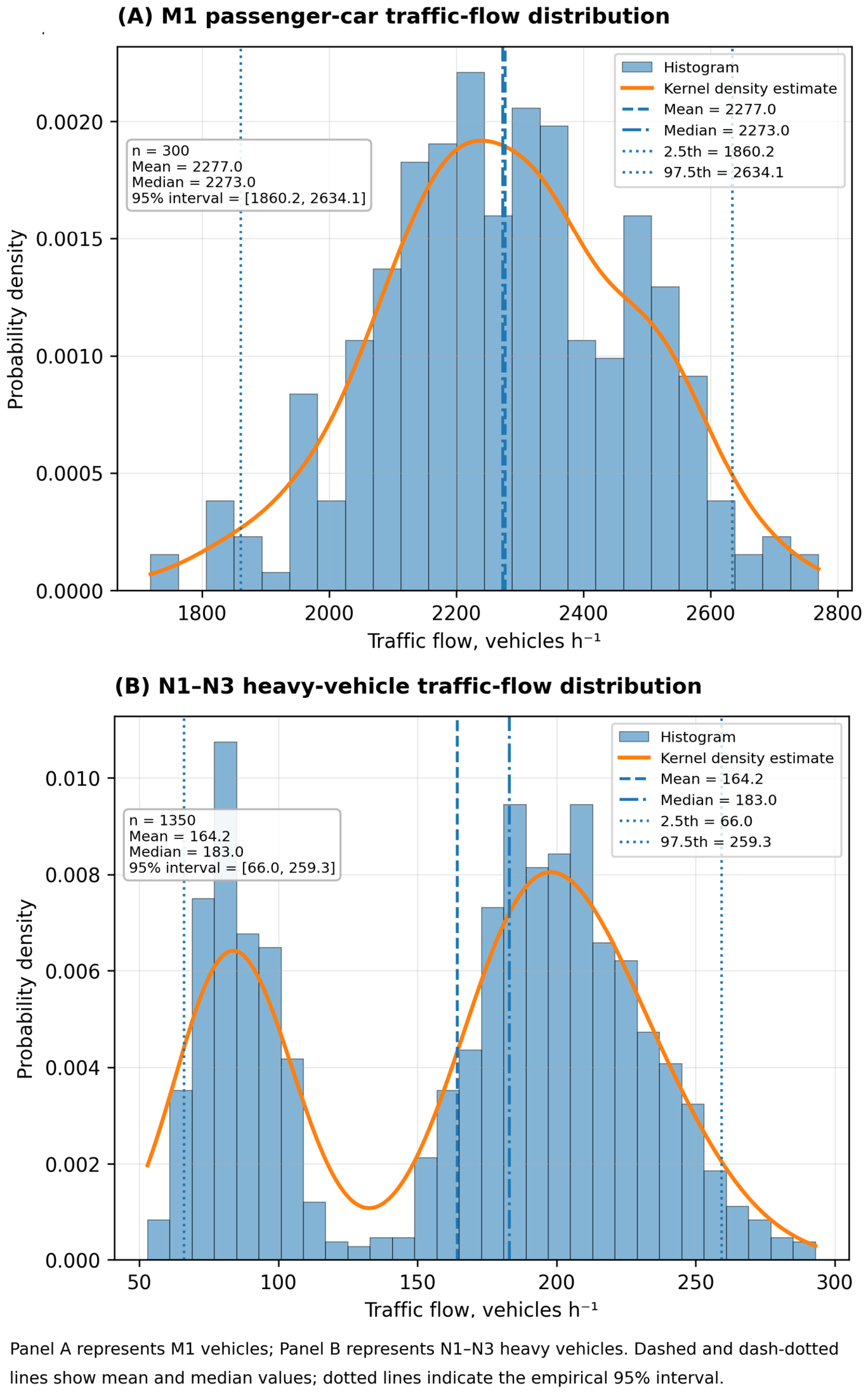
The probability distributions of traffic flows of class M1 passenger cars and heavy vehicles presented in Figure 1 allow us to assess not only the absolute difference in transport intensity between vehicle categories, but also the structural stability, variation and potential impact of the flows themselves on the formation of emissions in the transport system. The distribution of M1 transport flows seen in Part A of the figure is characterized by a shape relatively close to a normal distribution, the central part of which is concentrated in the interval ~2200–2350 veh h⁻¹.

Traffic-flow observations were generated using probability distributions fitted to the selected empirical ranges. Distribution parameters were chosen to reproduce realistic traffic variability and to avoid excessive concentration near boundary values. The resulting synthetic datasets therefore preserve the statistical characteristics of plausible transport-flow regimes while enabling systematic uncertainty analysis.

Meanwhile, the distribution of heavy vehicles presented in Part B is clearly more heterogeneous and characterized by two pronounced maxima, allowing us to identify different transit transport modes. In the case of M1 transport flows, the average value reaches 2277 veh h⁻¹, and the median—2273 veh h⁻¹; therefore, the difference between the central tendency indicators is minimal. This indicates a fairly symmetrical distribution and a relatively stable structure of passenger-car traffic on the section under consideration. The empirical 95% interval from ~1860 to ~2634 veh h⁻¹ additionally confirms that even in the presence of traffic variation, the main state of the transport system remains concentrated around the average value. From an engineering point of view, such a distribution is typical of urbanized arterial corridors dominated by periodically recurring weekday mobility patterns. The relatively small variance also allows us to assume that the dynamics of M1 flows mainly depend on the general urban mobility demand, and not on random logistical or transit processes. On the other hand, even in the presence of a relatively stable structure of M1 flows, a slight broadening of the distribution observed on the right side of the histogram in the ~2450–2600 veh h⁻¹ zone indicates the possible formation of a saturated traffic regime. In such conditions, even a small additional increase in traffic can disproportionately affect emissions due to more frequent braking–acceleration cycles, reduced average speed, and increased idling time. The literature has repeatedly shown that emissions are not linearly proportional to traffic intensity alone, as traffic dynamics and traffic regimes also play a significant role. Therefore, even a relatively homogeneous M1 distribution can shift to a significantly less efficient regime if the transport system approaches the capacity limit.

Meanwhile, the distribution of heavy vehicles has a fundamentally different structure. The average N1–N3 flow value is about 164 veh h⁻¹, but the median reaches ~183 veh h⁻¹, which means that the distribution is not symmetrical. The clear bimodality that is visible allows the identification of at least two separate heavy-vehicle regimes. The first maximum is concentrated in the range of ~70–100 veh h⁻¹ and can be associated with periods of lower transit activity or partial restriction of heavy vehicles. The second maximum at ~180–220 veh h⁻¹ indicates a more intensive transit transport regime, characteristic of active periods of logistics and interregional movement.

This bimodal structure is particularly important from the perspective of emission modeling, as it shows that heavy vehicles in the system do not function as a constant background flow but as a periodically activated intensive emission generator. The literature discusses a relatively small number of studies showing how such a structure directly relates to the disproportionate impact of heavy vehicles on air pollution. Heavy vehicles can generate a significant share of CO₂, NOx, and social costs, and particulate matter due to higher specific emission factors, higher mass, and lower energy efficiency.

It is also important to note that the left part of the heavy vehicles’ distribution has a longer “tail,” which indicates greater regime instability. This means that heavy-vehicle flows are more sensitive to changes in logistics, infrastructure, or regulation. This feature has major repercussions for transit transport management. Even small interventions, such as time restrictions or transit diversion, can fundamentally change the structure of heavy-vehicle flows and, accordingly, the distribution of emissions.

Analyzing both distributions together reveals a fundamental disproportion of the transport system: M1 transport dominates in absolute traffic volume, but heavy-vehicle modes are characterized by significantly greater structural variability and potentially greater emission sensitivity. Such a combination creates the prerequisites for a situation where the total traffic intensity remains relatively stable, but the total environmental impact can fluctuate significantly depending on the share of heavy vehicles. It is this disproportion that becomes one of the main reasons why heavy-vehicle management is considered in the literature as one of the most effective measures for reducing emissions and external social costs of urbanized corridors.

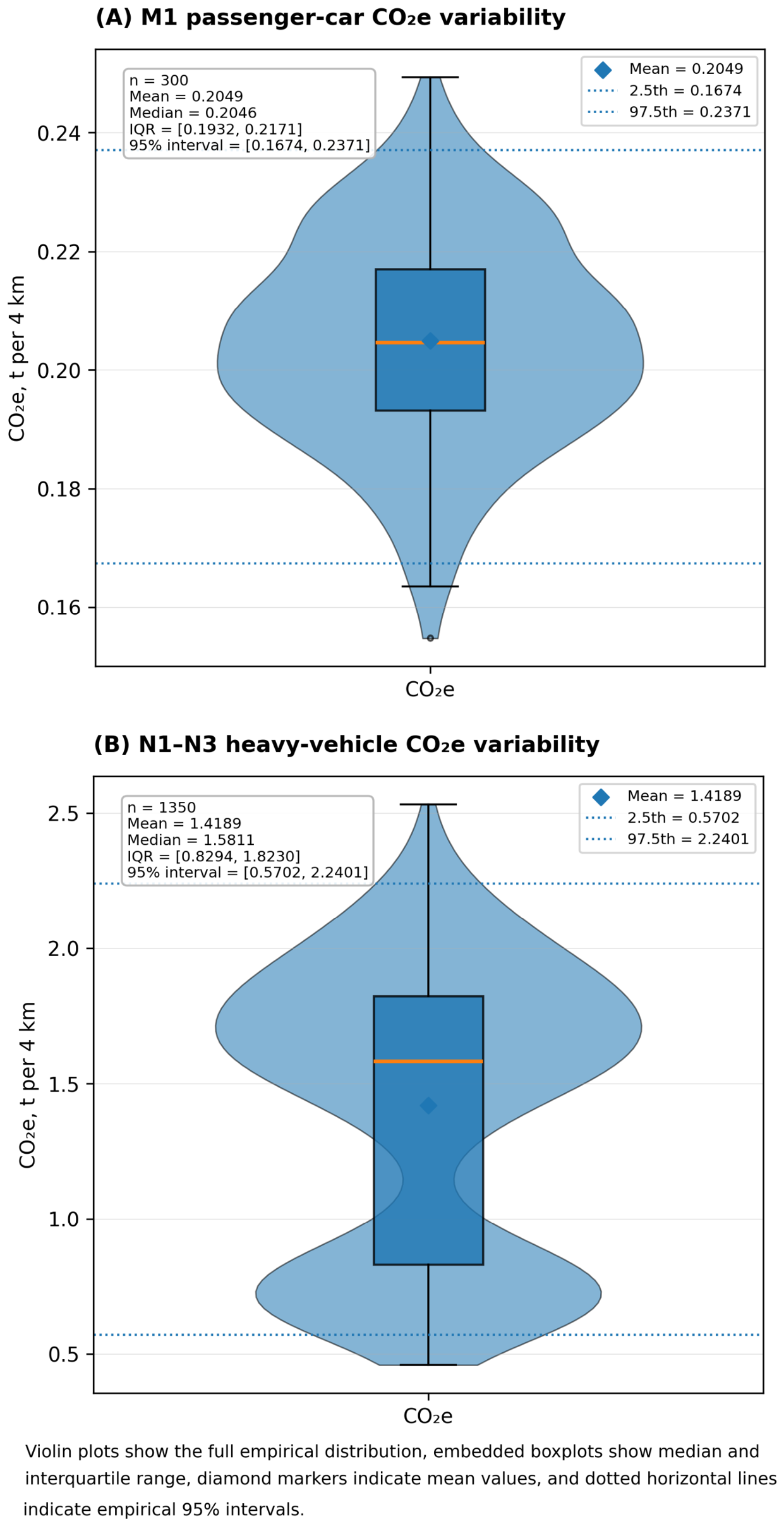
The assessment of the variability in the distribution of CO₂e emissions presented in Figure 2 allows for a comprehensive comparison of the climate impact created by M1-class passenger cars and heavy vehicles not only in terms of absolute emission values but also in terms of emission stability, dispersion structure, and probabilistic regimes. Unlike average classical analyses, violin-type diagrams allow for the simultaneous identification of central tendency, dispersion, distribution density, and possible signs of multimodality. Such a methodology is particularly important in transport-emission studies, since the real impact of the transport system is formed not only from the average emission value but also from the heterogeneity of regimes, peak states, and uncertainty.

The CO₂e distribution of M1 transport presented in Part A of Figure 2 is characterized by a rather narrow variation range and is relatively close to a unimodal distribution. The mean value of CO₂e is about 0.205 t/4 km, and the median is 0.2046 t/4 km, so the central tendency indicators practically coincide. This indicates a stable and slightly asymmetric emission regime. The interquartile range from ~0.193 to ~0.217 t additionally confirms that the majority of M1 emission values are concentrated in a narrow interval around the mean. Such a structure is typical of systems where emission generation mainly depends on relatively even traffic intensity and a homogeneous vehicle fleet. It is important to note that the violin shape of the M1 distribution does not have pronounced secondary maxima or longer asymmetric tails; therefore, it can be stated that the emission regimes of light vehicles are quite homogeneous. In practical terms, this means that the dynamics of M1 transport emissions primarily depend on the overall traffic intensity and average movement regime, rather than on individual extreme states. Such an emissions structure is more favorable in terms of modeling stability, since there are fewer probabilistic “jumps” in the system that could cause disproportionate short-term increases in emissions.

On the other hand, even with a relatively narrow distribution of M1, the 95% interval from ~0.167 to ~0.237 t indicates that the emission amplitude can differ by more than 40% between the lowest and highest regimes. This means that even emissions from light vehicles are not completely stable and are sensitive to changes in traffic conditions. The literature has repeatedly shown that even small changes in speed and acceleration in dense urban traffic can significantly affect emission factors, especially when moving from steady movement to a saturated braking–acceleration regime.

Meanwhile, the distribution of CO₂e for heavy vehicles presented in Part B has a fundamentally different structure. First of all, the significantly higher absolute scale of emissions is obvious—the average CO₂e value reaches about 1.42 t/4 km, i.e., almost seven times more than in M1 transport. However, the shape of the distribution itself is even more important. Unlike in the M1 case, the violin diagram of heavy vehicles is characterized by a pronounced bimodality, with one maximum forming in the ~0.7–0.8 t zone, and the second in the ~1.6–1.8 t interval.

Such a double density maximum indicates that the heavy-vehicle emission system functions in at least two different operational modes. The first mode can be associated with periods of lower intensity transit transport or more efficient movement, when flows remain more even. The second mode most likely reflects more intensive logistical states, higher load, more frequent acceleration cycles and higher fuel consumption. Such a structure directly corresponds to the sensitivity of heavy vehicles to traffic regime, speed and load changes described in the literature.

The very large dispersion of heavy vehicles is particularly significant. The interquartile range from ~0.83 to ~1.82 t indicates a very wide range of emissions, while the 95% interval from ~0.57 to ~2.24 t confirms that there are very different emission regimes in the system. From an engineering point of view, this means that heavy-vehicle emissions are significantly more sensitive to the condition of the infrastructure, speed regime, congestion, acceleration cycles and load changes than passenger car emissions. It is also important to note that the mean for heavy vehicles (~1.42 t) is lower than the median (~1.58 t), which indicates an asymmetric distribution with a longer “tail” of low emissions. Such a structure means that the system periodically exhibits relatively efficient heavy-vehicle regimes, but most of the emissions are concentrated in the zone of higher values. This is why even a relatively small reduction in heavy-vehicle traffic can generate a disproportionately large reduction in total CO₂e.

Analyzing both transport categories together reveals a systemic disproportion between traffic stability and emissions stability. Although M1 transport generates a higher total traffic load, its emissions distribution remains relatively homogeneous. Meanwhile, heavy vehicles are characterized not only by higher absolute emissions, but also by much greater mode heterogeneity. This means that heavy vehicles become the main source of uncertainty in system emissions. It is this feature that explains why heavy-vehicle management is often identified in the literature as one of the most effective measures for reducing both climate impact and external social costs in urbanized transport corridors.

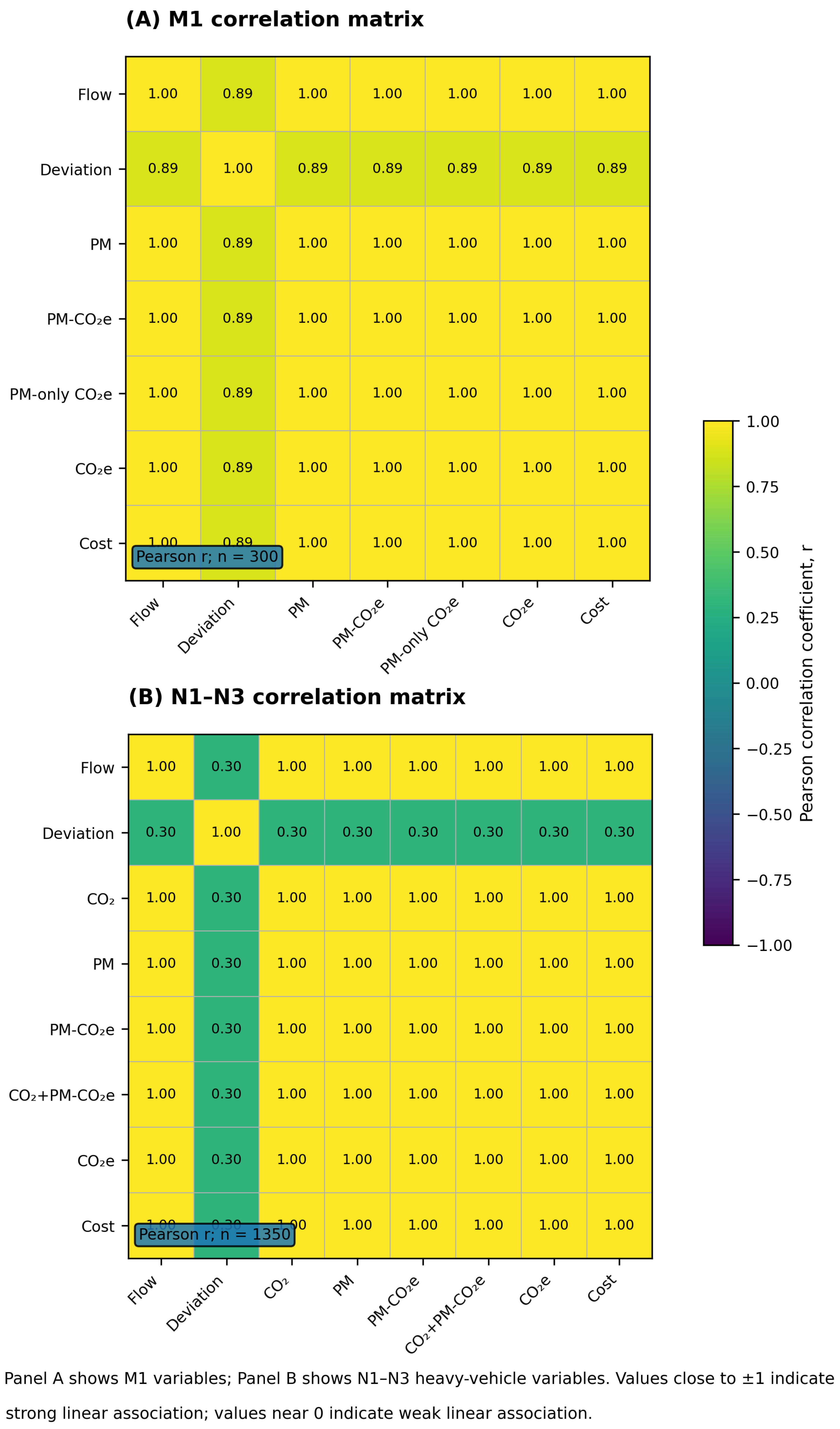
The Pearson correlation structure between traffic flow, emissions and financial impact indicators presented in Figure 3 allows for a systematic assessment of the interdependencies between the main variables of the model and for identifying which parameters have the greatest impact on the formation of CO₂e and the economic costs of pollution. The correlation matrix should primarily be interpreted as an assessment of internal model consistency rather than as independent empirical evidence of causal relationships. Because several variables are mathematically linked through the model structure, strong correlations are expected and provide confirmation that the emission, climate-impact and economic modules remain internally coherent.

It is important to note that several variables included in the correlation analysis are not statistically independent. The CO₂e indicator is partially derived from CO₂ and PM emissions, while financial pollution costs are directly calculated from CO₂e using a fixed valuation coefficient. Consequently, very high correlation coefficients are partly a structural consequence of the modeling framework itself. The correlation analysis is therefore used primarily to verify internal consistency and variable propagation throughout the analytical chain rather than to establish independent empirical relationships.

The correlation matrix for class M1 passenger cars presented in Part A of Figure 3 shows an extremely strong interdependence of almost all variables. Most of the Pearson correlation coefficients reach r ≈ 1.00, which means an almost ideal linear dependence between traffic flow, particulate matter (PM), PM-to-CO₂e transformation, total CO₂e and financial cost indicators. This result shows that in the M1 emissions system, the main factor in the formation of emissions is the transport intensity itself, and all other emission indicators are largely derived deterministically from changes in flow.

From an engineering point of view, this means that the M1 emissions model is characterized by very high structural stability. As the flow of passenger cars increases, both PM, CO₂e, and the financial impact of pollution increase almost proportionally. Such a situation is typical for homogeneous transport flows, in which the vehicle fleet is relatively homogeneous, and the operating modes do not differ radically. In other words, M1 transport emissions depend mainly on the quantitative traffic intensity, and not on mode changes or specific operating conditions.

However, it is important to note that such high correlation coefficients also indicate a possible multicollinearity problem. Since most indicators are almost perfectly correlated with each other, from a statistical point of view they convey very similar information. This means that when developing regression or predictive models, some of these parameters may be redundant. On the other hand, this result is not unexpected, as emissions in the M1 system were calculated using relatively constant emission factors, so the overall change in CO₂e directly inherits the flow dynamics.

The only slightly lower correlation coefficient (~0.89) is observed between the flow deviation and the other variables. This indicates that the deviation parameter does not reflect the absolute amplitude of emission generation, but rather the relative instability of the flow. Such a feature is important for interpreting the sensitivity of the system to short-term changes in the traffic regime. Even if the overall M1 emission pattern remains very stable, local flow fluctuations can still affect the instantaneous emission dynamics.

Meanwhile, the correlation matrix for heavy vehicles presented in Part B has a much more complex structure. Although very strong correlations are also observed between the main emission indicators (r ≈ 1.00), the significantly reduced relationship between the flow deviation and the other parameters (r ≈ 0.30) indicates a much greater heterogeneity of the heavy-vehicle modes. This is one of the most important results of Figure 3.

This relatively weaker relationship means that the heavy-vehicle emissions system is not a purely linear flow function in M1 transport. Unlike in M1 transport, here the formation of emissions is significantly influenced by additional factors: load, speed regime, acceleration cycles, logistics nature, differences in vehicle types and traffic organization conditions. Therefore, even a heavy-vehicle flow of similar intensity can generate significantly different emissions.

It is particularly important that the heavy-vehicle emission indicators maintain a very high mutual correlation between CO₂, PM and financial costs. This means that the impact of heavy vehicles on the system is not only large in absolute terms, but also systematically propagates through the entire emission chain—from primary pollutants to economic impact. Such a structure confirms the disproportionate role of heavy vehicles in pollution of urban and regional transport systems, often emphasized in the literature.

The correlation of financial costs with CO₂e and PM indicators also remains practically ideal. This shows that the economic impact model is very sensitive to changes in emissions and that even a relatively small reduction in heavy-vehicle emissions can lead to a disproportionately large reduction in economic damage. Such dependence is particularly important when assessing the effectiveness of transit transport restriction policies. When analyzing both matrices together, it becomes obvious that the M1 and N1–N3 transport systems have different emission generation logics. In the case of M1 transport, the emissions structure is more deterministic and stably dependent on the volume of traffic, while the heavy-vehicle emissions system is much more sensitive to regime changes and structural heterogeneity. This feature explains why heavy vehicles regulation measures are often identified in the literature as one of the most effective strategies for reducing both CO₂e emissions and the social costs of pollution.

From a methodological point of view, the figure also confirms that the emissions model used maintains internal consistency between the flow, emissions and economic impact links. At the same time, it reveals that in the case of heavy vehicles, the macroscopic flow parameter alone is not sufficient to fully explain emissions; therefore, detailed regime modeling becomes a prerequisite for an accurate analysis of the impact of transit transport.

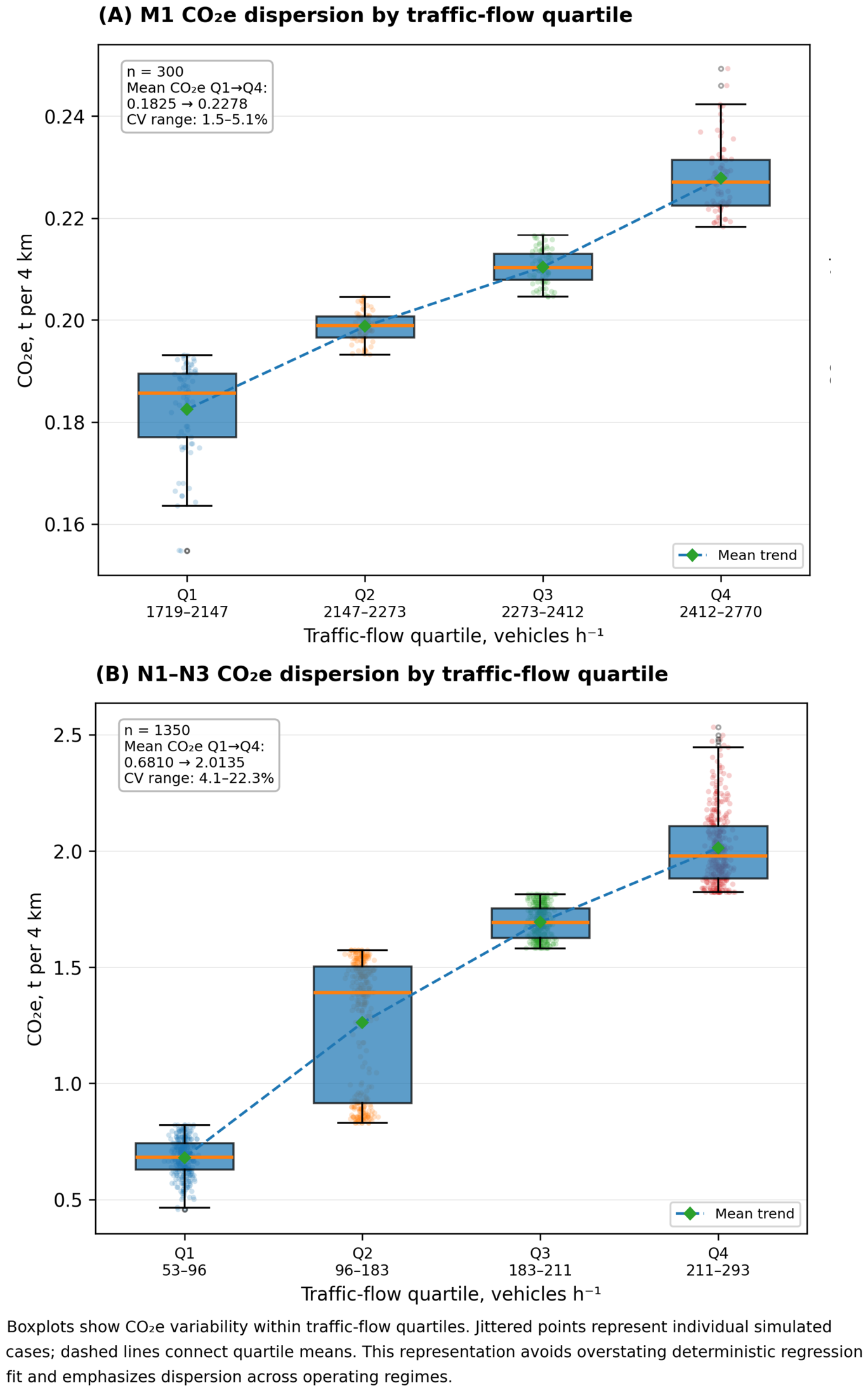
The sensitivity and variance analysis of CO₂e emissions by traffic-flow quartiles presented in Figure 4 allows us to assess how emissions dynamics change when moving from lower to higher traffic intensity regimes. Unlike classical regression dependencies, this analysis focuses not only on the average emission trend, but also on the internal variability, stability and probabilistic dispersion of each traffic regime. Such an approach is particularly important in transport emissions research, because in real systems emissions are often formed not according to a single deterministic function, but as a result of several regimes and different operational states.

The CO₂e dispersion of class M1 passenger cars by traffic-flow quartiles presented in Part A of Figure 4 shows a fairly consistent and close to linear emission growth trend. The average emission values from the first to the fourth quartile increase from ~0.1825 to ~0.2278 t/4 km, which corresponds to about a 25% increase in emissions with increasing transport intensity from the lowest to the highest traffic regimes. This trend indicates a relatively stable response of emissions to traffic changes, typical of a more homogeneous passenger-car transport regime. It is important to note that the boxplot structure remains quite compact within each quartile. The interquartile ranges are relatively narrow, and the number of outliers is small. This indicates that M1 transport emissions remain quite stable and insensitive to random mode changes even with increasing traffic. The range of the coefficient of variation (CV) from ~1.5 to ~5.1% further confirms the low internal uncertainty of emissions. This emission structure shows that the formation of emissions in the passenger car system depends mainly on the total volume of transport, and not on complex operational regimes or a highly heterogeneous composition of the transport fleet.

On the other hand, when moving to the fourth quartile, a slightly more pronounced increase in dispersion and more high-value outliers are visible. This allows us to assume that less stable traffic regimes begin to form as the network load approaches. In such states, even small additional growth in traffic can lead to a disproportionate increase in emissions due to more frequent acceleration–braking cycles and a decrease in average speed. The literature has repeatedly shown that it is precisely in saturated traffic conditions that emissions begin to increase at a faster rate than the flow itself.

However, the overall response of M1 emissions remains quite consistent and monotonous. The average values between quartiles increase gradually, which indicates that the passenger car emission system is characterized by relatively high predictability. This feature is important both for model validation and for planning emission reduction measures, since even at higher flows it is possible to predict the expected change in emissions with sufficient accuracy.

Meanwhile, the heavy-vehicle CO₂e dispersion presented in Part B of Figure 4 has a fundamentally different structure. First of all, a significantly larger absolute scale of emissions is visible—the average value of the fourth quartile exceeds 2.0 t/4 km, i.e., it is almost ten times higher than the M1 fourth quartile value. However, the dispersion dynamics themselves are even more important.

In the first quartile, heavy-vehicle emissions remain quite concentrated at the ~0.6–0.8 t interval, but already in the second quartile a very pronounced increase in dispersion is visible. It is in this regime that one of the most important points of system instability is formed. The boxplot structure becomes much wider, a larger amplitude of values appears, and the coefficient of variation reaches significantly higher values than in M1 transport. The CV range from ~4.1 to ~22.3% indicates that the heavy-vehicle emissions system is very sensitive to regimes.

This phenomenon has a clear engineering interpretation. Heavy-vehicle emissions strongly depend not only on the traffic intensity, but also on the operating conditions: load, speed regime, road profile, acceleration cycles and the technological condition of vehicles. Therefore, even a heavy-vehicle flow of similar intensity can generate very different emissions. It is for this reason that the heavy vehicles system develops a much larger dispersion of emissions than in the case of passenger cars.

Of particular importance is the trajectory of average emissions between the third and fourth quartiles. Although emissions continue to increase, their growth rate becomes less uniform, and the dispersion remains large. This indicates that the system is moving into a more saturated regime, in which an additional increase in traffic no longer leads only to a proportional increase in emissions, but also creates additional instability. This structure directly corresponds to the sensitivity of heavy vehicles to congestion, low-speed regimes and frequent acceleration cycles described in the literature.

It is also important to note that in the case of heavy vehicles, even in the lower quartiles, the dispersion of emissions remains larger than in the fourth quartile of M1. This indicates that the very nature of heavy vehicles leads to greater uncertainty in emissions. In practical terms, this means that regulating heavy vehicles can have a disproportionately large impact not only on average emissions, but also on their stability.

When considering both transport categories together, it becomes clear that the M1 emissions system is relatively deterministic and predictable, while the N1–N3 system is characterized by strong regime heterogeneity. These results indicate that emission dispersion increases nonlinearly across heavy-vehicle traffic regimes, highlighting the importance of regime-dependent emission management.

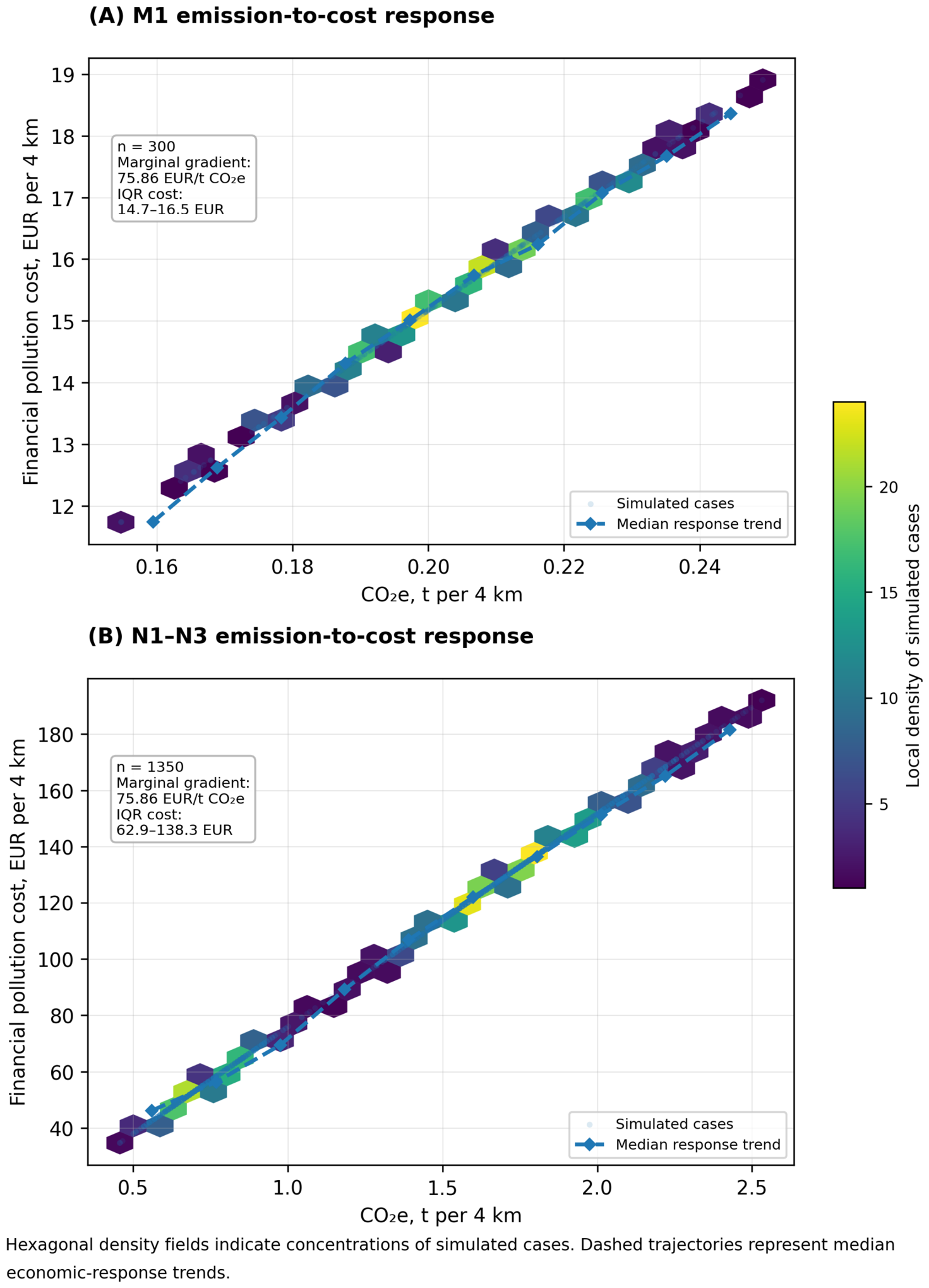
The dependence of the economic impact of pollution on CO₂e emissions presented in Figure 5 allows us to assess how changes in emissions are transformed into financial external costs in different transport categories. The analysis of emission intensity, economic impact and probability density combined in the figure allows us not only to identify the general emission-cost dependence, but also to assess the sensitivity of the system to different emission regimes. Such an analysis is particularly important in the assessment of transport policy, as it allows us to move from physical emission indicators to the interpretation of social and economic consequences.

The emission-cost response of class M1 passenger cars presented in Part A of Figure 5 shows a very consistent and almost linear dependence between the amount of CO₂e and the financial costs of pollution. As emissions increase from approximately 0.15 to 0.25 t/4 km, the financial costs increase consistently from ~12 to ~19 EUR/4 km. The presented marginal gradient (~75.86 EUR/t CO₂e) shows that each additional ton of CO₂e in the system generates relatively constant additional economic damage. Such an almost deterministic dependence indicates that the economic impact of M1 transport depends mainly on the total amount of emissions, and not on specific regime effects.

Hexagonal density analysis additionally allows us to identify the most likely states of the system. The highest density of points is concentrated at ~0.18–0.21 t CO₂e and ~14–16 EUR intervals; therefore, it can be stated that the majority of M1 emissions generate a relatively medium-sized economic impact. At the same time, the density structure remains quite narrow, which means that there are no pronounced economic extremes or abrupt transitional regimes in the system. Such a structure is characteristic of a homogeneous urban passenger-car flow, in which the dynamics of emissions fairly directly inherit changes in the flow.

However, even this relatively stable structure shows a clear sensitivity of the economic impact to the growth of emissions. For example, an increase in CO₂e from ~0.18 to ~0.24 t/4 km leads to an increase in financial damage of more than 4 EUR/4 km on a stretch. On a systemic scale, such differences become significant, especially in dense urban corridors where transport flows are constantly repeated. This means that even relatively small changes in emissions can create disproportionately high external costs in the long term.

It is also important to note that the median trajectory curve almost perfectly follows the overall density structure. This indicates a high stability of the economic model and low sensitivity to random fluctuations in emissions. In other words, the economic impact of M1 transport is quite predictable and increases quite evenly with increasing emission levels. Such a feature is important when planning emission reduction measures, as it allows for a fairly accurate forecast of the expected scale of economic benefits from reducing passenger car emissions.

Meanwhile, the heavy-vehicle emissions–cost relationship presented in Part B is of a much larger scale and has much more important systemic implications. The CO₂e range for heavy vehicles is around 0.4–2.5 t/4 km, and the corresponding financial costs increase to ~190 EUR/4 km. This means that the absolute economic impact of heavy vehicles is more than ten times higher than the financial damage caused by M1 vehicles.

Of particular importance is that although the marginal gradient remains the same (~75.86 EUR/t CO₂e), the total impact of heavy vehicles becomes disproportionately large due to much higher emissions. The results demonstrate that economic externalities scale more rapidly with heavy-vehicle emission intensity than with passenger-car activity. In other words, the disproportion of economic impact does not arise from a different cost factor, but from a much larger scale of emissions.

The hexagonal density structure in Part B is also much wider than in the M1 case. The highest concentration of points is observed at ~1.4–1.9 t CO₂e and ~110–150 EUR intervals, but the system clearly shows greater dispersion and longer “tails” of high values. This means that the economic impact of heavy vehicles is characterized by much greater regime heterogeneity. Even relatively small changes in the heavy-vehicle regime can significantly affect the overall scale of economic damage.

The shape of the median trajectory also shows that as emissions increase, the economic impact consistently increases. However, unlike in M1 transport, in the heavy vehicles system, the greater dispersion of emissions also implies greater economic uncertainty. In practical terms, this means that the regulation of heavy vehicles can have a disproportionately large impact not only on the average amount of emissions, but also on the stability of the economic impact of the entire system.

It is also important to pay attention to the interquartile range of costs. In the case of M1 transport, it is only ~14.7–16.5 EUR, while in the heavy vehicles system the range increases to ~62.9–138.3 EUR. This means that the economic damage of heavy vehicles is characterized not only by a larger absolute scale, but also by a much higher variance. Such a feature is especially important when assessing transit transport management policies, since even a partial reduction in heavy-vehicle traffic can significantly reduce not only the average economic damage, but also the probability of extreme pollution costs. When analyzing both transport categories together, it becomes obvious that the economic impact of emissions in the system is strongly disproportionate. Although M1 transport generates a larger share of the total traffic, heavy vehicles become the main source of financial pollution damage. It is this disproportion that explains why restrictions on heavy vehicles are often identified in the literature as one of the most effective measures for reducing both emissions and social external costs in urbanized transport corridors.

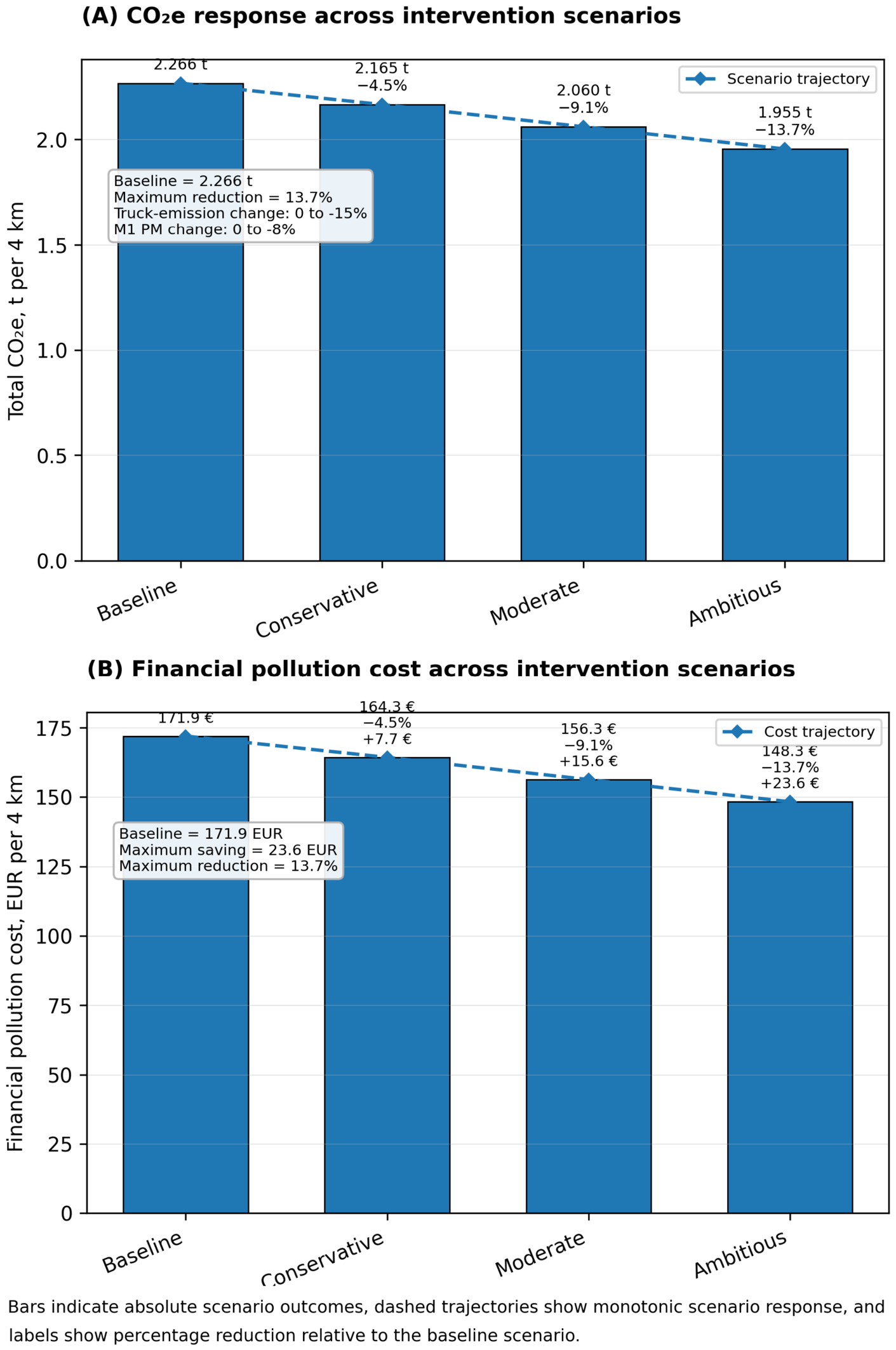
The scenario analysis presented in Figure 6 allows us to assess how different intensities of transit transport restriction measures affect the total CO₂e emissions and the financial costs of pollution. Unlike the previous figures, which mainly analyzed the internal structure of the system and the dynamics of emissions, this stage moves on to assessing the effectiveness of interventions. Part A of the figure presents the change in total CO₂e between the baseline, conservative, medium and ambitious scenarios, and Part B analyzes how these emission changes are transformed into the economic impact of pollution.

Part A of Figure 6 shows a clear monotonic trajectory of emission reduction with increasing intensity of interventions. In the baseline scenario, the total CO₂e amount reaches about 2.266 t/4 km, but when moving to the conservative scenario, it decreases to ~2.165 t/4 km, to ~2.060 t/4 km in the medium scenario, and to ~1.955 t/4 km in the ambitious scenario. This means that the measures taken allow for a reduction in the total amount of CO₂e by approximately 13.7% compared to the initial state.

It is important to note that the emission reduction between the scenarios remains quite consistent. This result indicates that the modeled system is characterized by a relatively stable response to transit transport restriction measures. In other words, each additional level of intervention generates the predicted emission reduction, and the system does not show sudden non-linear jumps or emission “collapse” effects. This is an important result from an engineering point of view, as it shows that even gradually implemented measures can generate tangible climate benefits.

At the same time, this trajectory also allows us to identify a trend of relatively decreasing efficiency. Although the emission reduction between the scenarios remains stable in percentage terms, the absolute size of the additional benefit gradually decreases. This means that the system begins to approach a regime in which each additional restriction measure generates an increasingly smaller additional emission reduction. Such a trend in transport systems is often associated with the “diminishing returns” effect, when the initial stage of restrictions eliminates the most emission-generating modes, and further regulation already affects relatively more efficient flows.

It is particularly important that the combination of interventions presented in the figure include not only the reduction in heavy-vehicle emissions (up to −15%) but also changes in M1 particulate matter (up to −8%). This shows that the emission reduction effect is formed as a result of the interaction of several components of the transport system. Such a structure corresponds to the need to assess transport policy in a comprehensive manner, emphasized in the literature, since restrictions in one category often spread to other links in the system.

When analyzing the amplitude of the emission reduction itself, it becomes obvious that even a relatively small percentage reduction in absolute terms can have a significant impact on the climate impact balance. For example, in an ambitious scenario, the emission reduction exceeds 0.31 t CO₂e/4 km. When considering longer transport corridors and permanent transit flows, such an effect can be transformed into a very significant annual reduction in emissions.

The response of the financial costs of pollution to the scenario changes presented in Part B of Figure 1 largely replicates the emission reduction trajectory but provides an additional economic interpretation. In the baseline situation, the financial costs amount to about 171.9 EUR/4 km, but in the conservative scenario they decrease to ~164.3 EUR, in the medium scenario to ~156.3 EUR, and in the ambitious scenario to ~148.3 EUR. In this way, the maximum reduction in financial damage reaches about 23.6 EUR/4 km.

This economic dynamic is particularly important from the point of view of transport policy, as it allows the transformation of the climate impact into a directly interpretable socio-economic indicator. In other words, emission reduction measures not only reduce the physical amount of CO₂e but also generate direct economic benefits in the form of lower external costs. Such an interpretation is particularly important when assessing the effectiveness of restrictions at the municipal or regional level, where decision-makers often focus not only on the amount of emissions, but also on the financial benefits.

It is also important to note the very consistent trajectory of the decline in economic costs. Since the financial model in this study is directly linked to the CO₂e indicator, the cost decline curve maintains an almost identical structure to the emissions curve. However, from a practical point of view, the economic effect becomes much easier to interpret than CO₂e quantities alone. For example, a reduction of EUR 23.6 in one 4 km section may seem small at first glance, but at the scale of the transport network and in multiple transit modes such differences transform into a significant overall reduction in social costs.

It is additionally important to note that the trajectories of both emissions and economic costs remain monotonic and do not have anomalous jumps. This indicates high stability of the model and relatively good consistency of scenarios. Such a feature is important when assessing the predictability of policy measures. If the system were to exhibit strong nonlinear effects or abrupt tipping points, the consequences of transit transport regulation would be much more difficult to predict.

When analyzing both parts of the picture together, it becomes clear that even relatively limited transit transport interventions can generate a disproportionately large reduction in the overall climate and economic impact. This is especially important considering that heavy vehicles make up a relatively small share of total traffic but generate a significant amount of emissions and social costs. It is precisely because of this disproportion that restrictions on transit heavy vehicles are often considered in the literature as one of the most effective measures to reduce the climate and economic impact of urban and regional transport corridors.

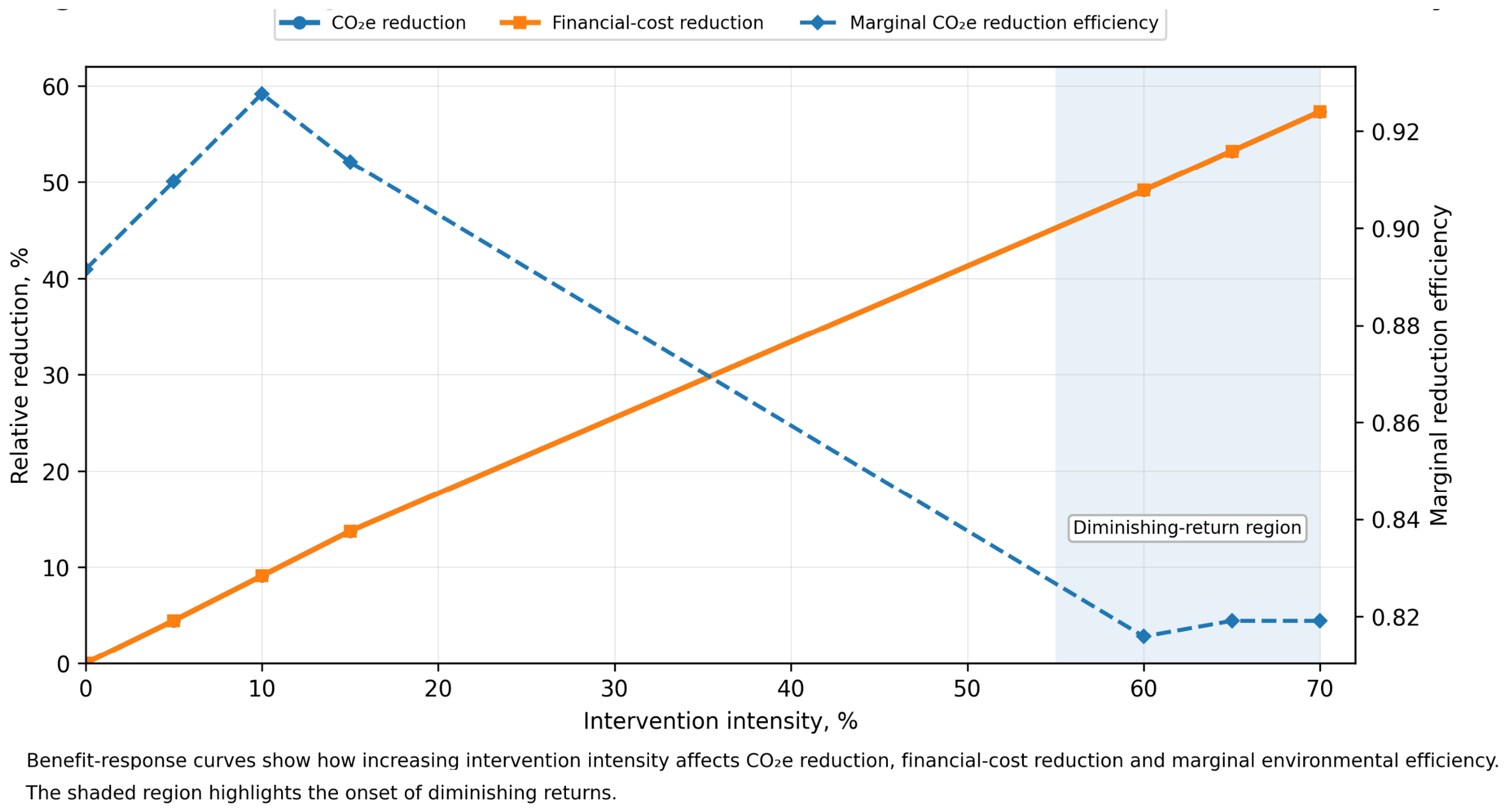
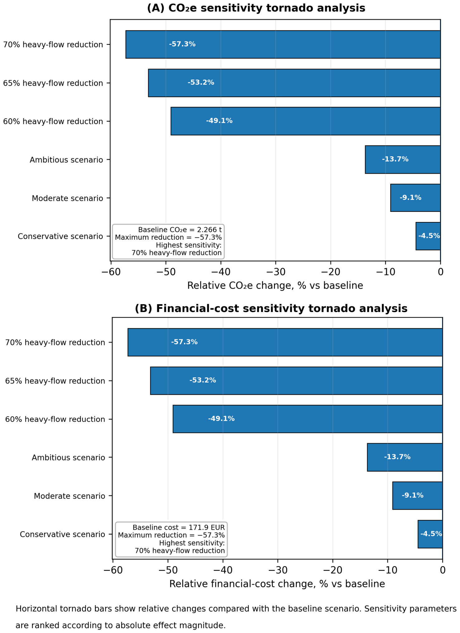
The analysis presented in Figure 7 should be interpreted as a comparative ranking of intervention sensitivities rather than a classical bidirectional tornado analysis. The objective was to compare the relative magnitude of emission and cost reductions generated by different intervention scenarios with respect to the baseline condition. The 60%, 65% and 70% heavy-flow reduction cases were not treated as independent model parameters. Instead, they represent alternative intervention scenarios included to illustrate the response of the system under progressively more restrictive heavy-vehicle management assumptions. Such analysis is extremely significant in the modeling of transport systems, as it allows us to identify which regulatory factors have the largest systemic effect and which generate only limited additional benefits.

The CO₂e sensitivity analysis presented in Part A of Figure 7 shows a very clear disproportion in the impact of interventions. The largest effect is generated by aggressive heavy-vehicle flow restrictions—60%, 65% and 70% heavy-flow reduction scenarios. The maximum emission reduction reaches about −57.3%, which is more than four times greater than in the most ambitious variant of the general intervention scenario. This result shows that the system’s emission dynamics are particularly sensitive to the intensity of heavy vehicles.

From an engineering point of view, this disproportion is logical. The analysis of the previous figures showed that N1–N3 transport is characterized not only by a much higher absolute amount of CO₂e, but also by a significantly higher regime heterogeneity. Therefore, even a partial reduction in heavy-vehicle traffic eliminates the most emission-inefficient regimes. In other words, the system first eliminates the highest intensity emission segments, so the overall effect becomes disproportionately large.

It is particularly important that the 60–70% heavy-vehicle restriction scenarios create an almost exponential emission reduction effect, while the conservative, medium and ambitious scenarios cause relatively moderate changes—from about −4.5 to −13.7%. This shows that general emission reduction measures aimed at the entire transport system generate a limited effect if they are not directly targeted at heavy vehicles. This conclusion is in good agreement with the structural disproportion between the share of heavy vehicles in the flow and its contribution to total pollution described in the literature.

It is also important to note the structure of the tornado diagram itself. Since the bars are arranged according to the absolute magnitude of the effects, it becomes obvious that the system has one clearly dominant intervention scenario—the intensity of heavy-vehicle flow. This means that the model is characterized by a high concentric dependence on one main group of emissions. Such a property is extremely important when planning policy measures, as it allows directing interventions to the most effective link in the system.

On the other hand, such a distribution of sensitivity also indicates the potential vulnerability of the system. If the dynamics of emissions depend too strongly on one transport segment, even small changes in the logistics system can significantly affect the overall climate balance. This is especially relevant in the areas of ports, logistics corridors or international transit nodes, where heavy-vehicle flows are characterized by high time and mode variability.

The sensitivity analysis of financial costs presented in Part B of the figure essentially replicates the structure of CO₂e sensitivity. The maximum reduction in financial damage also reaches about −57.3%, and the sensitivity hierarchy remains practically identical. This indicates a very strong dependence of the economic impact on the amount of emissions. In other words, financial damage in the system directly inherits changes in emissions, so emission reduction measures are automatically transformed into economic benefits.

This dependence has an important methodological significance. Since the structure of the sensitivity of the economic impact almost perfectly replicates the sensitivity of emissions, it can be stated that the economic coefficients used in the model maintain a high internal consistency. This means that the financial assessment is not random or independent of the dynamics of emissions, but functions as an integrated part of the emissions system.

It is particularly important that the amplitude of the sensitivity of the financial impact becomes very large precisely in the case of aggressive heavy-vehicle restrictions. This means that the regulation of transit transport generates not only climatic, but also significant economic benefits. From a practical point of view, such a conclusion is of great importance for municipal and regional planning institutions, as it allows them to base emission reduction measures not only on environmental but also economic efficiency.

It is also significant that the conservative scenario leads to a reduction in financial costs of only about −4.5%. This indicates that minimal interventions may not be sufficient to achieve tangible economic benefits. In other words, there is a certain threshold of interventions in the system, below which the impact remains limited. Such a tendency is characteristic of many complex transport systems, in which emission regimes are strongly related to the flow structure and the logistics network.

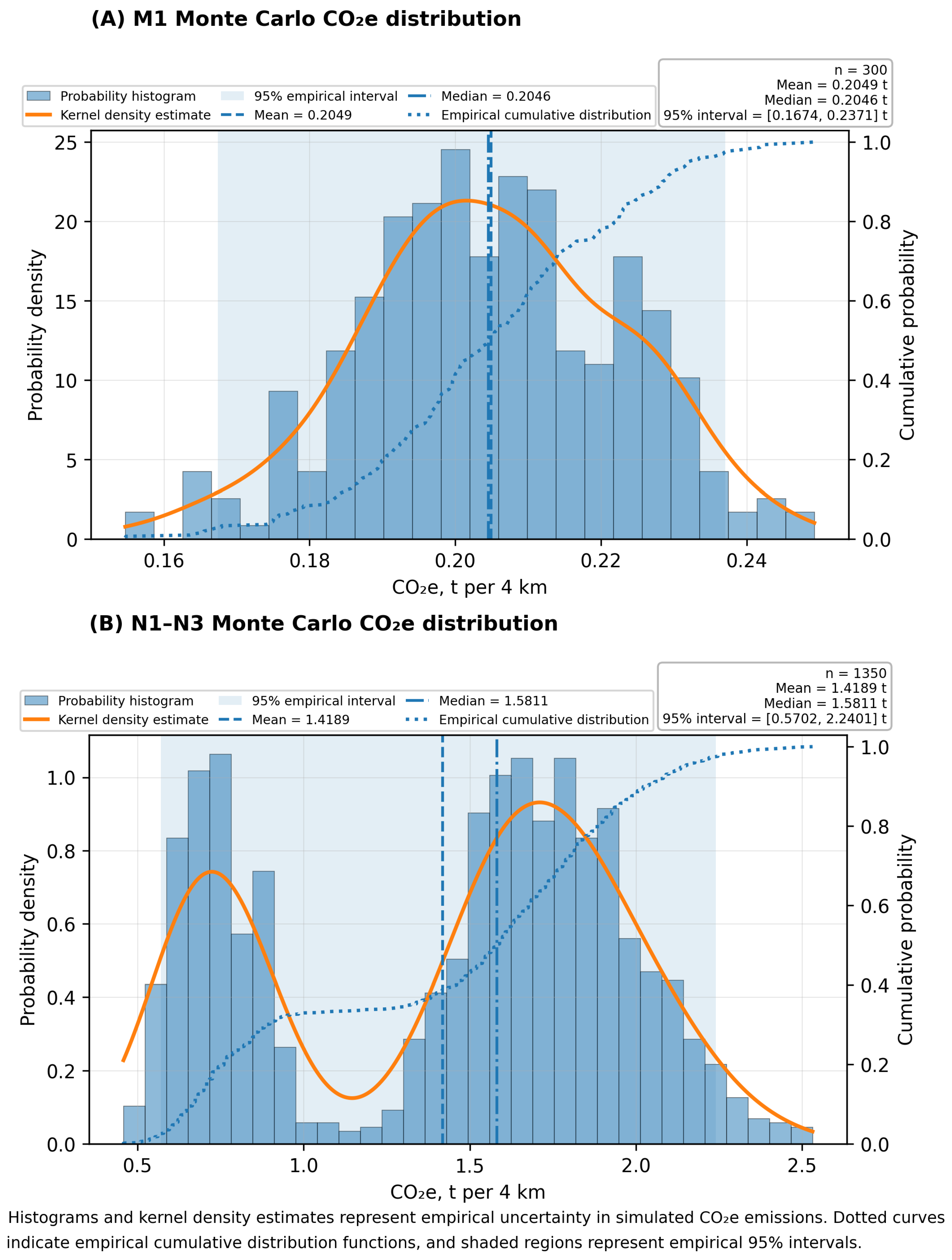
The Monte Carlo-type analysis of the distribution of CO₂e emissions presented in Figure 8 allows us to assess not only the average emission values, but also their probability structure, uncertainty and risk amplitude in different transport categories. Unlike the previous figures, which were dominated by deterministic or scenario assessment, this analysis focuses on the stochastic interpretation of the system. Such a methodology is particularly important in the modeling of transport emissions, since real traffic systems are characterized by high regime variability, which is determined by the dynamics of transport flows, logistical chains, meteorological conditions and heterogeneous operation of vehicles. The probability distribution of CO₂e for M1-class passenger cars presented in Part A of the figure shows a rather narrow and relatively homogeneous emission structure. The average CO₂e value is about 0.2049 t/4 km, and the median is ~0.2046 t/4 km; therefore, the central tendency indicators practically coincide. This result indicates very low asymmetry and a fairly stable emission regime. The histogram and the nuclear density function (KDE) curve show a single dominant maximum at ~0.20–0.21 t, suggesting that most of the states of the M1 system are concentrated around one main operating mode.

The empirical 95% interval from ~0.167 to ~0.237 t additionally shows that even the more extreme emission states remain relatively close to the central tendency. In other words, the M1 emission system is characterized by relatively low stochastic uncertainty. From an engineering point of view, such a structure is typical of homogeneous urban passenger-car flows, where the emission dynamics depend mainly on the overall traffic intensity and to a lesser extent on individual operating anomalies.

The empirical cumulative distribution function (CDF) curve additionally confirms this stability. The curve increases quite evenly and does not have sharp jumps, so the probability of transitioning to extreme emission modes remains relatively small. In practical terms, this means that the M1 transport emissions system is highly predictable and has a relatively low risk of generating very high emission values. This feature is important both for model validation and for planning long-term emission reduction strategies.

However, even this relatively stable structure shows some sensitivity to higher emission regimes. The right-hand “tail” of the KDE curve at ~0.22–0.24 t suggests that emissions may increase disproportionately during saturated traffic or more intense braking–acceleration regimes. The literature has repeatedly shown that even passenger car emission factors are sensitive to changes in the flow regime, especially with decreasing average speed and increasing short-term acceleration cycles.

Meanwhile, the Monte Carlo-type distribution of heavy vehicles presented in Part B of the figure has a fundamentally different and much more complex structure. First of all, the much larger absolute scale of emissions is obvious—the average value reaches about 1.4189 t/4 km, and the median is even ~1.5811 t/4 km. The difference between the average and the median indicates an asymmetric distribution and an increased influence of low emission values on the average value.

Even more important is the shape of the distribution itself. Unlike in the case of M1, the KDE curve for heavy vehicles is characterized by clear bimodality. One maximum form exists in the ~0.6–0.8 t zone, and the second at the ~1.6–1.9 t interval. This result indicates that the heavy-vehicle emissions system functions in at least two different operational modes. The first mode is likely related to lower intensity or more efficient transit movement, while the second reflects a more intensive logistics mode, higher load and more frequent acceleration cycles.

Of particular importance is the very wide amplitude of the 95% interval—from ~0.57 to ~2.24 t. This means that the heavy-vehicle emissions system is characterized by very high stochastic uncertainty. From a practical point of view, this shows that even with a similar heavy-vehicle flow, real emissions can differ several times depending on specific operating conditions. Such a feature is especially important when assessing the impact of transit transport on urbanized corridors, since “hot states” of very high emissions can periodically form in the system.

The shape of the CDF curve additionally confirms this heterogeneity. Unlike M1 transport, the cumulative function of heavy vehicles is characterized by uneven growth and pronounced transition zones between different modes. This means that there are relatively clear groups of emission states in the system, and the transition between them is not uniform. Such a structure is characteristic of complex logistics systems, in which emission modes are strongly affected by loads, speed modes, the infrastructure condition and transport organization features.

It is also important to note that the right “tail” of the heavy-vehicle distribution remains quite long. This means that there is a relatively small, but significant, probability of very high emission regimes in the system. Such regimes are usually associated with low speed, congestion or high load states. The literature has repeatedly shown that heavy vehicles are disproportionately sensitive to such regimes, especially in infrastructure nodes and logistics corridors.

When analyzing both transport categories together, it becomes obvious that the M1 system is characterized by a relatively stable and predictable distribution of emissions, while the N1–N3 system becomes the main source of emission uncertainty. It is the bimodality of heavy vehicles and the wide risk interval that determines that the overall climate impact of the system becomes sensitive to changes in transit transport regimes.

Such a structure has very important practical implications. Since the heavy-vehicle emissions system is characterized by high uncertainty and the probability of high emission regimes, even partial regulation of heavy vehicles can not only reduce average emissions, but also significantly reduce the risk of extreme emission states. It is this characteristic that explains why in the literature, heavy-vehicle management is often identified as one of the most effective measures for reducing both the overall climate impact and emission uncertainty in urban and regional transport networks.

An important advantage of the proposed framework compared with conventional deterministic transport-emission approaches is its ability to quantify uncertainty and emission-risk distributions rather than relying solely on average values. Deterministic models typically provide a single expected emission estimate for a given traffic state, whereas the probabilistic framework additionally characterizes variability, exceedance probabilities and the likelihood of extreme-emission regimes. Consequently, the framework enables risk-oriented policy assessment and supports decision-making under uncertainty, which cannot be directly achieved using traditional average-value methodologies.

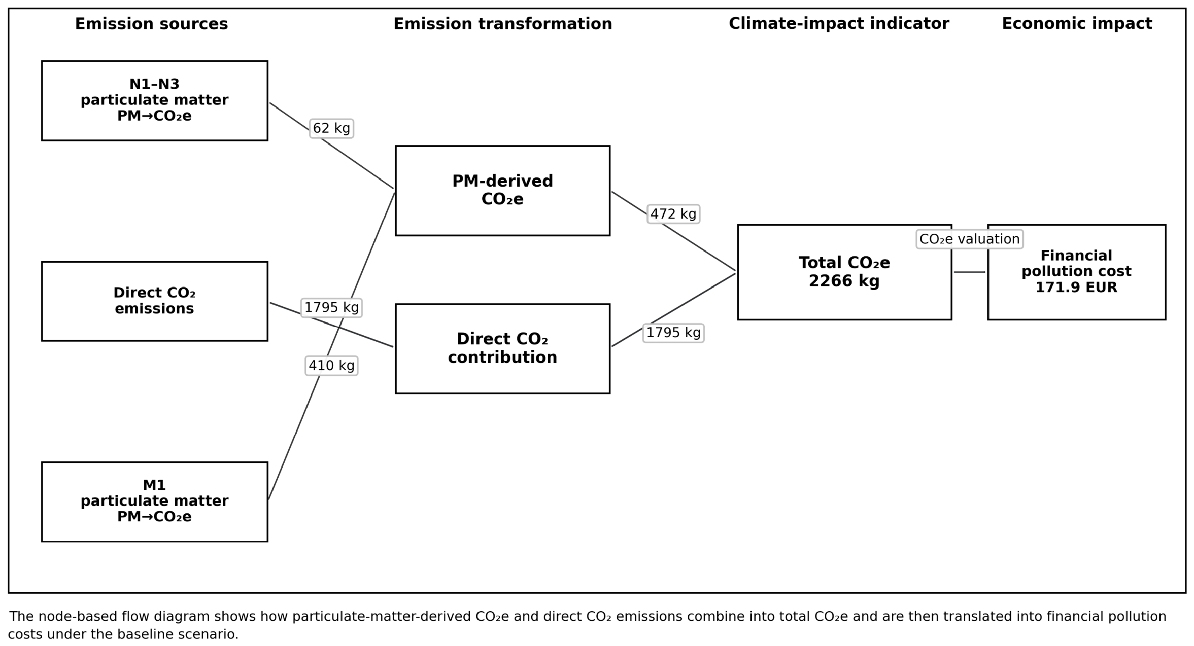
The node-based scheme of transport emissions, CO₂e formation and economic impact presented in Figure 9 allows for a systematic representation of the entire structure of the emissions chain under consideration—from primary pollution sources to the final economic impact. Unlike previous figures, which were dominated by statistical or probabilistic analysis, this scheme focuses on a systematic interpretation of causal relationships. Such a representation principle is particularly important in transport system research, as it allows us not only to identify the main emission sources, but also to show how different emission components are transformed into an aggregated climate impact indicator and subsequently into economic damage. The main emission sources are presented on the left side of the scheme: the heavy-vehicle particulate matter (PM to CO₂e), direct CO₂ emissions and the M1 transport PM-to-CO₂e component. This arrangement allows for a clear identification that the system under consideration is not based solely on direct CO₂ assessment. On the contrary, the total climate impact is formed as the sum of several emission links, where the conversion of particulate matter into CO₂ equivalent also plays an important role.

At first glance, the larger PM-derived CO₂e contribution associated with M1 vehicles may appear counterintuitive given the higher per-vehicle emission intensity of heavy vehicles. However, this result reflects the substantially larger traffic volume of M1 vehicles within the analyzed system. While heavy vehicles generate considerably higher emissions on a per-vehicle basis, the cumulative PM-derived contribution from the much larger passenger-car fleet exceeds that of the heavy vehicles segment. Consequently, Figure 9 represents aggregate system-level contributions rather than vehicle-specific emission intensities.

Of particular importance is that the diagram clearly shows the disproportion between different emission components. Direct CO₂ emissions amount to about 1795 kg and are the dominant source of the total climate impact. Meanwhile, the CO₂e components of PM origin are significantly smaller—about 62 kg in the heavy vehicles segment and about 410 kg in M1 transport. However, even the relatively smaller PM → CO₂e contribution remains significant in the structure of the overall system, since particulate matter is often associated with additional local health impacts and higher social costs in urbanized areas.

From an engineering point of view, this disproportion is very important. It shows that although the climate impact balance is dominated by direct CO₂ from fuel combustion, the contribution of particulate matter is not insignificant and must be integrated into the overall emission assessment. This methodology is consistent with the modern direction of transport emissions modeling, where the impact of emissions is assessed not only in terms of the direct amount of carbon dioxide, but also in terms of a wider spectrum of climate and health impacts.

The emissions transformation chain presented in the central part of the diagram additionally allows us to understand how the primary emission sources are combined into a common climate impact indicator. The PM-derived CO₂e node shows that the impact of particulate matter in the system is not assessed separately but is transformed into the form of CO₂ equivalent. This is a methodologically important step, as it allows us to unify the impact of different pollution components on the overall climate measure.

The value of 472 kg PM-derived CO₂e becomes particularly important here. Although it constitutes only a part of the total amount of CO₂e, its existence shows that the climate impact in the system is not only the result of direct combustion emissions. From a practical point of view, this means that CO₂ reduction measures alone do not necessarily ensure the maximum climate effect if particulate matter emissions are not also reduced. It is for this reason that the importance of integrated emissions management is increasingly emphasized in the literature.

The overall climate impact indicator presented on the right side of the diagram—total CO₂e 2266 kg—reflects the final integrated result of the system’s emissions. This node becomes the main intersection point of all previous links. This means that the overall climate impact in the system is not formed as the result of a single component, but as a complex sum of several emission links. Such a structure reflects the nature of modern transport emission systems, where the impact of pollution is multilayered and strongly dependent on the interaction of transport modes.

The last part of the chain, where CO₂e is transformed into the financial impact of pollution, is particularly significant. The financial pollution cost node, reaching about 171.9 EUR, shows that physical emissions in the system are directly converted into economic damage. Such a transformation gives the model an extremely important practical dimension. Emissions become not only a physical environmental indicator, but also a socio-economic parameter that can be used to assess the effectiveness of policies.

From a causal point of view, the diagram very clearly shows the logic of the emissions chain. Transport flows generate primary emissions, which are transformed into an aggregated CO₂e indicator, which in turn creates a financial impact. However, it is important that this causal chain is not just mathematical. It reflects a real systemic mechanism, where changes in transport modes directly affect not only the climate balance, but also social and economic losses.

It is also important to note the structure of the diagram itself. Emission sources, the transformation chain, the climate impact indicator and the economic impact are arranged sequentially from left to right. Such an arrangement not only improves visual clarity but also allows the system to be interpreted as a single emissions-impact chain. This is particularly important in transport policy analysis, as it allows for a clear identification of where interventions could generate the greatest effect in the system.

When analyzing the whole scheme together, it becomes clear that the main source of climate and economic impact in the system remains direct CO₂ emissions, but the PM-to-CO₂e component also contributes significantly to the overall impact. This structure explains why reducing total transport flow alone is not necessarily the most effective strategy. Selective management of the modes and transport segments generating the highest emission intensity becomes much more important, especially focusing on heavy vehicles and modes with high PM intensity.

Although synthetic datasets cannot fully substitute long-term field observations, they provide an effective means of evaluating uncertainty propagation, sensitivity structures and scenario responses in complex transport emission systems. The purpose of the present study was therefore not to reproduce a specific measured corridor but to examine how different traffic regimes influence climate impacts and external pollution costs within a probabilistic modeling environment. Nevertheless, future validation against observed traffic-flow datasets remains an important step for further development of the framework.

4. Discussion

The present study was not designed as a benchmarking exercise against a specific deterministic transport-emission model. Consequently, the results should not be interpreted as evidence that probabilistic approaches universally outperform deterministic methodologies. Instead, the framework is intended to complement conventional approaches by providing additional information regarding uncertainty, variability and emission-risk distributions that are typically not represented in average-value assessments. The estimated emission reductions associated with aggressive heavy-vehicle restrictions represent direct first-order responses of the modeled system. They do not account for secondary behavioral adaptations such as route diversion, temporal rescheduling, freight consolidation, modal substitution or induced demand effects. Previous studies from Bogotá and São Paulo have demonstrated that such adaptation mechanisms may partially offset expected environmental benefits. Therefore, the reported 57% reduction should be interpreted as a theoretical upper-bound response within the assumptions of the present framework rather than a guaranteed real-world outcome.

The high-restriction scenarios involving 60–70% reductions in heavy-vehicle flows should be interpreted as exploratory policy experiments rather than realistic short-term implementation targets. In practice, achieving such reductions would require substantial changes in freight organization, logistics networks, modal distribution and corridor management strategies. Potential responses could include traffic redistribution to alternative routes, temporal rescheduling of freight movements, consolidation of shipments, increased use of rail transport or adoption of lower-emission vehicle technologies.

Consequently, the environmental benefits estimated under the most restrictive scenarios should be viewed as indicative upper-bound responses within the modeling framework. Real-world outcomes would likely depend on behavioral adaptation, infrastructure capacity, regulatory feasibility and the ability of logistics operators to reorganize freight flows while maintaining service levels.

The interpretation of the correlation analysis requires particular caution. Because several variables are linked through deterministic model equations, the resulting correlation structure reflects both the underlying transport–emission relationships and the mathematical dependencies embedded within the framework. Therefore, the correlation matrix should be interpreted primarily as evidence of internal model coherence and variable propagation rather than as standalone empirical validation of transport-system behavior.

The results should be interpreted in the context of methodological integration rather than methodological invention. The objective of the study was not to develop a new probabilistic algorithm, but to demonstrate how multiple established analytical approaches can be systematically combined to evaluate climate impacts, uncertainty propagation and economic externalities of heavy-vehicle flows. In this respect, the framework provides a systems-level assessment tool that links engineering, environmental and economic dimensions that are often analyzed separately in previous studies.

The analysis of the probability of exceeding CO₂e emissions presented in the Section 4 allows us to move from a deterministic assessment of emissions to an interpretation of risk and uncertainty. Unlike the statistical distributions or sensitivity analyses presented in the Section 3, this graph focuses on the probabilistic risk of emissions under different intervention scenarios. This approach is particularly important in the assessment of transport policy, since the management of real systems is usually based not only on average values, but also on the probability of exceeding certain critical limits.

The probability of exceeding probability curves presented in Figure 10 show how the probability of exceeding a certain CO₂e level changes when moving from the baseline to the conservative, medium and ambitious scenarios. The horizontal axis reflects the CO₂e limit in t/4 km format, and the vertical axis represents the probability that the system will exceed this emission limit. Such a representation allows us to interpret the transport system not as a single fixed emission state, but as a probabilistic process in which the risk of different emission regimes exists.

The baseline scenario has the highest probability of exceedance over almost the entire CO₂e range. The curve remains close to the 1.0 to approximately 2.0 t threshold, which means that in the current state of the system the probability of exceeding the 2.0 t CO₂e level is very high. Even at the ~2.2 t threshold, the probability of exceedance remains significant, which indicates a strong tendency of the system to form high-intensity emission regimes. Such a structure reflects the heterogeneity of heavy-vehicle emissions identified in the previous figures and the existence of high emission states.

The 2.0 t CO₂e policy threshold marked in the graph is particularly important. This value acts as a critical control point for the system, allowing us to assess how many different scenarios reduce the probability of exceeding the environmentally undesirable emission level. In the baseline scenario, the probability of exceedance at this threshold remains very high; therefore, it can be stated that the current structure of the transport system is characterized by insufficient climate impact stability.

A clear reduction in risk is visible when moving to the conservative scenario. The curve shifts to the left, which means that the same emission limit becomes less likely. However, even in the case of conservative measures, the system remains quite sensitive to higher emission regimes. This shows that partial or relatively weak restrictions on transit transport can reduce average emissions, but do not effectively eliminate the highest risk regimes.

The average scenario is characterized by a much more pronounced reduction in the probability of exceedance. The curve becomes steeper and approaches zero more quickly at higher CO₂e values. This shape indicates not only lower average emissions, but also a significantly reduced probability of high emission states. In practical terms, this means that the system becomes more stable and less sensitive to unfavorable operating regimes.

The ambitious scenario generates the largest effect. The curve in this scenario is shifted the most to the left, so even relatively low CO₂e limits become unlikely to be exceeded. At 2.0 t, the probability of exceeding the threshold decreases to a relatively small level, and the probability of higher emission states practically approaches zero. This shows that more aggressive transit transport management measures not only reduce the total amount of emissions, but also significantly reduce the climate risk of the system.

From an engineering point of view, the shift in the curves to the left has a very clear interpretation. It means that the system is moving to a lower emission regime and that high emissions become statistically less likely. This feature is especially important in urbanized transport corridors, where short-term episodes of high emissions often lead to disproportionate impacts on air quality and public health.

It is also important to note the shape of the curves themselves. The baseline scenario is characterized by a relatively slower decrease in probability, which indicates greater regime heterogeneity. Meanwhile, the curve of the ambitious scenario is steeper and more concentrated. This means that interventions not only reduce average emissions but also narrow the range of possible system states. In other words, the system becomes not only “cleaner”, but also more stable.

This type of analysis is particularly valuable in the context of transport policy, as it allows decision-makers to assess not only the average change in emissions, but also the expected reduction in climate risk. The literature increasingly emphasizes that it is precisely the reduction in risk and uncertainty that is becoming one of the most important criteria for the management of sustainable transport systems.

When analyzing all the curves together, it becomes obvious that transit transport interventions affect not only the overall level of emissions, but also the risk structure of the system itself. More ambitious scenarios significantly reduce the likelihood of entering high-climate-impact regimes; therefore, such measures can be interpreted as strategies not only for reducing emissions, but also for increasing climate stability. It is this feature that explains why, in the literature, the regulation of heavy vehicles is often considered one of the most effective measures for reducing both climate impact and emission uncertainty in urban and regional transport systems.

The presented marginal benefit analysis allows us to assess how the increasing intensity of transit transport interventions affects not only the overall emission reduction, but also the effectiveness of the measures themselves. Unlike the scenario analysis presented in the Section 3, which is mainly focused on absolute changes in emissions and financial costs, this graph focuses on the dynamics of the effectiveness of interventions. Such analysis is particularly important in the assessment of transport policy, as it allows us to identify the threshold from which additional regulatory measures begin to generate diminishing additional benefits.

Figure 11 presents three main trajectories: relative CO₂e reduction, reduction in financial pollution costs and marginal emission-reduction efficiency. The horizontal axis reflects the intervention intensity in percentage terms, while the left vertical axis shows the overall relative reduction in emissions and financial costs. The right vertical axis presents marginal environmental efficiency, which allows us to assess how much additional benefit is created by increasing the scale of interventions.

The trajectory of CO₂e reduction shows a fairly consistent reduction in emissions with increasing intervention intensity. When moving from the 0 to 70% intervention level, the total emission reduction approaches ~57–58%. This means that more aggressive heavy-vehicle restrictions and emission control measures can eliminate more than half of the total climate impact in the corridor under consideration. Such a result is very consistent with the disproportionate role of heavy vehicles in the emissions system identified in the previous figures.

It is particularly important that the emission reduction curve initially rises quite rapidly. Even with relatively small interventions of 5–15%, a clear CO₂e reduction effect is observed. This indicates that the system has the most inefficient modes in terms of emissions, which can be eliminated with relatively limited measures. From an engineering point of view, such dynamics mean that the transit transport system is highly sensitive to the initial regulatory stage.

However, as the intervention intensity increases, the growth rate of the curve gradually decreases. Although the total CO₂e reduction continues to increase, the amplitude of the additional benefits becomes smaller and smaller. It is this trend that is marked in the graph as the “diminishing-return region”. This zone, which starts at around 55–60% of the intervention level, indicates that the system is approaching the saturation point for emission reduction.

This effect is very important in the analysis of transport systems. It means that early interventions eliminate the most inefficient transport modes, but later measures already start to affect relatively more efficient flows. In other words, the more the system is optimized, the more difficult it is to achieve additional significant emission reductions. In the literature, such a trend is often associated with the operational efficiency limit, when additional interventions start to generate a smaller relative effect.

The curve of the decline in the financial costs of pollution almost perfectly repeats the trajectory of the decline in CO₂e. This indicates a very strong dependence of the economic impact on the amount of emissions. As the intensity of the intervention increases, the reduction in financial costs reaches almost the same extent as the reduction in emissions. In practical terms, this means that emission control measures are directly transformed into economic benefits in the form of lower external costs.

This dependence has a very important policy interpretation. Since the economic effect practically directly inherits the change in emissions, transport regulation measures can be justified not only by climatic but also by financial arguments. Such a feature is especially important in the context of municipal and regional planning, where the economic efficiency of measures often becomes one of the main decision-making criteria.

The marginal emission-reduction efficiency curve provides an additional systemic interpretation. In the initial stages of interventions, efficiency remains very high and even increases slightly. This shows that early measures are particularly effective, because they first eliminate the most polluting and inefficient transit transport modes. Such a structure corresponds very well to the strong dependence of the system on heavy vehicles identified in previous sensitivity analyses.

However, later, the marginal efficiency starts to decrease. At around the 60% intervention level, the efficiency curve reaches its lowest point and a further increase in interventions generates only very limited additional benefits. This means that the system is moving into a saturated emission control regime. Such dynamics are very important for planning real policy measures, as they allow identifying economically and technically rational levels of intervention.

The marked diminishing-return region is of particular practical importance. It shows that beyond a certain threshold, additional measures to restrict transit transport begin to generate fewer and fewer environmental benefits, although the costs of their implementation may continue to grow. Such a situation is often observed in complex transport systems, where the initial regulation eliminates the most obvious inefficiencies, but further optimization becomes much more complicated.

When analyzing all trajectories together, it becomes obvious that the efficiency of transit transport management is not infinite. Although larger interventions allow for greater emission reductions, there is a clear limit in the system, beyond which the additional benefit begins to decrease. Such a result is very important from both a methodological and practical point of view, because it allows us to move from the logic of purely reducing emissions to the search for the optimal balance of interventions.

It is this feature that explains why the importance of optimal, rather than maximum, transit transport control is increasingly emphasized in the literature. The most effective strategy is not the absolute elimination of transit, but the selective management of the highest-emission-intensity modes, which allows us to achieve the greatest climatic and economic benefits with the least additional intervention burden for the transport system.

The interpretation of heavy vehicles as a dominant emission source should be viewed within the context of the fleet assumptions adopted in the present framework. In practice, the environmental performance of heavy vehicles is increasingly influenced by technological modernization, electrification, alternative fuels and improved logistics management. Consequently, corridors characterized by a larger share of low-emission heavy vehicles may exhibit substantially different emission structures and intervention responses than those represented in the current analysis.

The proposed framework is designed to be transferable to other urban transport corridors because it relies on a modular structure consisting of traffic-flow inputs, emission factors, probabilistic uncertainty analysis and economic valuation modules. Application to another corridor would primarily require recalibration of traffic distributions, fleet composition parameters, corridor length and locally relevant emission factors. The analytical workflow itself remains unchanged. Therefore, the framework can be adapted to different urban, regional or transit-dominated transport systems while preserving methodological consistency.

5. Conclusions

This paper offers a summary of the key findings of the study and discusses its methodological and practical consequences. The conclusions are focused on the comparative involvement of M1 passenger vehicles and N1–N3 heavy vehicles in CO₂e emission creation, uncertainty propagation and external pollution costs. The section also describes the main contribution of the proposed probabilistic framework and the main limitations that should be addressed in any future study.

Within the assumptions of the analyzed fleet structure and emission factors, the modeling results suggest that heavy vehicles may generate a disproportionately large climate and economic impact compared with their share of total traffic activity.

The M1 transport system was characterized by a relatively homogeneous and close-to-normal distribution in emission regimes, while heavy-vehicle distributions demonstrated pronounced bimodality, large dispersion and high regime heterogeneity. This indicates that heavy-vehicle emissions strongly depend on operational conditions, traffic regime, load and logistics dynamics.

Correlation analysis confirmed a very strong direct dependence between transport flows, CO₂e emissions and financial pollution costs. However, the lower correlation between the flow deviation and emission parameters in the heavy vehicles segment showed that the macroscopic flow parameter alone is not sufficient to fully explain the emissions of transit transport. This confirms the need to apply a regime and probabilistic modeling approach.

Sensitivity analysis revealed that the largest systemic impact is generated by restrictions on heavy vehicles. Within the assumptions of the probabilistic framework, scenarios involving a 60–70% reduction in heavy-vehicle flows produced potential reductions exceeding 57% in total CO₂e emissions and pollution costs. These high-restriction scenarios were intended to evaluate the sensitivity limits of the modeled system and should therefore be interpreted as exploratory intervention cases rather than immediately implementable transport-policy targets. However, these estimates do not incorporate behavioral adaptation mechanisms and should therefore be interpreted as indicative upper-bound responses.

Monte Carlo analysis showed that heavy vehicles become the main source of uncertainty in system emissions. The N1–N3 segment is characterized by wide 95% emission intervals and long “tails” of high emission regimes, indicating a high probability of extreme emission states. Meanwhile, the M1 transport system remained much more stable and predictable.

Exceedance probability analysis showed that ambitious transit transport limitation scenarios significantly reduce the probability of exceeding critical CO₂e limits. This allows transport interventions to be interpreted not only as emission reduction measures, but also as strategies for reducing climate risk and system uncertainty.

Marginal benefit analysis identified a “diminishing-return” region at approximately 55–60% intervention intensity. This shows that after a certain threshold, additional transit transport limitation measures begin to generate increasingly smaller additional climate and economic benefits. Therefore, the most effective strategy is not maximum transit elimination, but optimized management of the highest emission intensity modes.

Integrated modeling, combining transport flows, PM-to-CO2e transformation, economic costs, probabilistic analysis and scenario modeling, allowed for a comprehensive assessment of the impact of transit transport in the urbanized corridor. The study demonstrates that multi-level statistical and probabilistic methods provide additional insight into uncertainty, emission variability and risk structures that are not explicitly represented in traditional aggregated transport-emission assessments.

The principal methodological contribution of this research is the development of an integrated assessment architecture that combines probabilistic emission modeling, climate-impact estimation, uncertainty quantification, sensitivity analysis and economic externality assessment within a single analytical workflow. While the individual analytical techniques are established in the literature, their combined application enables a more comprehensive evaluation of heavy vehicles’ impacts and supports evidence-based transport policy design under uncertainty.

The results obtained show that heavy-vehicle management can be one of the most effective measures to reduce CO₂e emissions, financial pollution costs and climate risk in urbanized transport corridors. At the same time, the study confirms the need to move from purely deterministic emission assessments to integrated risk, sensitivity and uncertainty analyses in the transport policy-making process.

Future development of the framework should include calibration against observed traffic-flow datasets, comparison with deterministic transport-emission models, integration of behavioral adaptation mechanisms and application across multiple transport corridors to evaluate transferability and generalizability.