WaveletMask: Wavelet-Domain Mask-Guided Degradation Detection for Old-Film Restoration

Abstract

Old films suffer from scratches, dust, and brightness flicker caused by aging film stock and unstable analog exposure. Recurrent restoration frameworks suppress these artifacts under the guidance of degradation masks, yet pixel-domain frame differencing provides weak evidence for thin structural defects and confuses global brightness variation with content change. We present WaveletMask, a wavelet-domain degradation sensing framework that disentangles these two failure modes by construction: a high-frequency branch localizes transient structural defects from Haar detail-band differences between adjacent frames, a low-frequency branch isolates frame-level brightness deviations from coarse approximation responses, and a parameter-free maximum fusion rule passes the dominant cue to the recurrent gate. On the Synthetic and Real-World Old Video (SRWOV) benchmark, WaveletMask attains the best PSNR among ten re-trained methods (26.60 dB, $+0.61$ dB over the strongest competitor), and a paired comparison against the Recurrent Transformer Network (RTN) confirms a $+0.45$ dB gain while adding only 898 detector parameters. On real archival footage, WaveletMask removes scratches and flicker more cleanly while better preserving film texture and temporal stability. These results indicate that explicit wavelet-domain separation of structural and photometric cues offers a reliable, nearly cost-free upgrade for mask-guided recurrent restoration.

1. Introduction

Preserving and restoring old films is essential for safeguarding the cultural and historical heritage embedded in moving images from earlier eras [1]. As physical film materials deteriorate through chemical decay, mechanical wear, and improper storage, digital restoration becomes a practical means of recovering damaged visual records [2]. In practice, old footage rarely exhibits a single isolated degradation. It typically combines spatially localized defects, such as scratches, dust, and blotches, with temporally varying photometric artifacts, such as brightness flicker and fading, as well as noise or grain introduced by aging and acquisition [3,4]. Because these degradations arise at different spatial and temporal scales, an effective degradation indicator should capture both high-frequency local anomalies and low-frequency frame-level variation, rather than relying solely on a single pixel-domain difference map.

Learning-based old-film restoration (OFR) has advanced rapidly with deep low-level vision models [5,6]. DeepRemaster [2] formulates spatiotemporal restoration with 3D convolutions and reference-based colorization. RTN [3] introduces bidirectional recurrent propagation with a learnable defect mask, where a pixel-domain degradation indicator gates the aggregation of propagated and current-frame features. RRTN [7] further improves alignment with recursive transformer blocks and second-order grid propagation. MambaOFR [8] replaces heavier restoration modules with efficient Mamba-based [9] components and degradation-aware prompting. Despite this progress, recurrent OFR still commonly relies on a spatial-domain frame-difference signal for gating [3]. Although attractive for its simplicity, such a signal is not equally sensitive to the mixed artifacts present in old films.

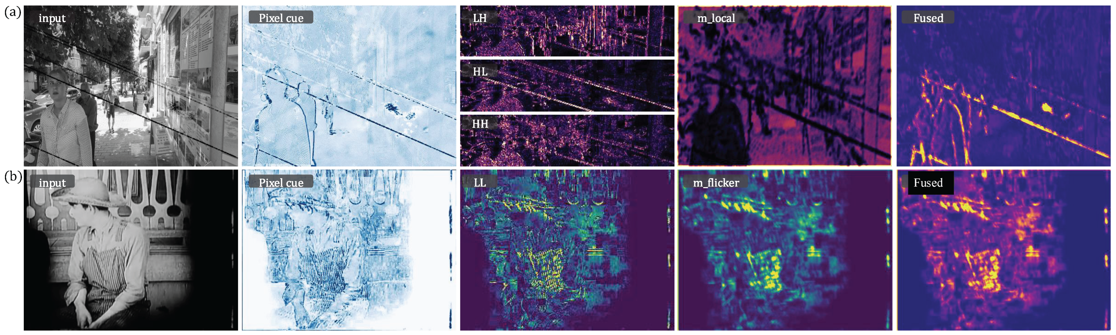
Figure 1 highlights the two cases that motivate this work. First, spatially sparse high-frequency damage, such as thin scratches and isolated dust, may affect only a small number of pixels and can therefore be diluted in a dense pixel-domain difference map. Second, brightness flicker is broad and low-frequency, often appearing as a near-uniform temporal offset that is difficult to disentangle from legitimate scene illumination changes using pixel differences alone. Treating these two regimes with the same detector can therefore yield an ambiguous gating signal for recurrent restoration.

Wavelet analysis offers a natural multi-resolution representation for separating these regimes [10]. The Haar discrete wavelet transform (DWT) decomposes an image into one low-frequency approximation band (LL) and three directional high-frequency detail bands (LH, HL, and HH). More broadly, wavelet coefficients have been used as localized damage evidence in signal-analysis detection settings, including continuous-wavelet-transform features coupled with sparse autoencoders [11]. Of course, wavelet coefficients are not semantic labels: motion boundaries and textured content can also activate detail bands. Even so, the decomposition provides a practical basis for OFR, because the high-frequency bands concentrate abrupt local discontinuities relevant to scratches and dust [12], whereas the LL band preserves coarse luminance structure that is informative for flicker. This frequency separation directly motivates the LHFM/GFM design adopted in this work.

Building on this motivation, we propose WaveletMask, a wavelet-domain degradation detection framework for recurrent OFR. The Local High-Frequency Mask Module (LHFM; Section 3.3) applies geometric-mean differencing to the Haar detail sub-bands to emphasize transient local damage. The Global Flicker Mask Module (GFM; Section 3.4) applies a minimum-difference temporal criterion to the LL sub-band to emphasize frame-level brightness changes. The two branch masks are then combined by an element-wise maximum to form the wavelet-domain gate used for recurrent aggregation. We also evaluate learned pixel-wise fusion with the original RTN spatial indicator as an ablation. However, it is not included in the proposed model because, under the tested training recipe, it underperforms the wavelet-only gate (

Table A11. Fusion strategy comparison on SRWOV synthetic data (Y-channel protocol). Checkmarks indicate included branches, and dashes indicate absent branches. WaveletMask with LHFM/GFM branch-level maximum fusion is the proposed model, and learned-fusion rows use the four-layer CNN recipe described in the text. All rows except the WaveletMask row are measured in one dedicated fusion-ablation evaluation run, in which the proposed configuration scores 26.6017 dB; the WaveletMask row displays the reference same-protocol value from Table A1, and the cross-run drift is below 0.002 on LPIPS and DISTS. In each metric column, the best result is in red and the second-best in blue.

Variant	LHFM	GFM	Fusion	PSNR ↑	SSIM ↑	LPIPS ↓	DISTS ↓
RTN	—	—	—	26.1580	0.8917	0.1034	0.0953
+LHFM	✓	—	direct	26.3778	0.8966	0.0914	0.0790
+LHFM + learned	✓	—	CNN	25.9858	0.8978	0.0889	0.0830
+GFM	—	✓	direct	26.1024	0.8980	0.0969	0.0916
+GFM + learned	—	✓	CNN	25.9488	0.8956	0.0946	0.0814
WaveletMask	✓	✓	max	26.6125	0.8954	0.0886	0.0827
WaveletMask + gated	✓	✓	gated CNN	26.3515	0.8966	0.0869	0.0842
WaveletMask + learned	✓	✓	max + CNN	24.9827	0.8896	0.1068	0.0867

). The overall pipeline is shown in Figure 2, and the two branches are detailed in Figure 3 and Figure 4.

The main contributions are as follows:

• WaveletMask: frequency-aware gating for recurrent OFR. We formulate degradation sensing in the Haar wavelet domain and replace a single pixel-domain difference gate with a two-branch design that separately models high-frequency local damage and low-frequency flicker cues.
• LHFM for transient structural defects. LHFM applies geometric-mean differencing to the LH, HL, and HH sub-bands across three consecutive frames, emphasizing frame-specific scratches, dust, and other local defects while suppressing responses from persistent edges and one-sided temporal changes.
• GFM for frame-level brightness instability. GFM applies a minimum-difference criterion in the LL sub-band to detect current-frame brightness deviations relative to both temporal neighbors, yielding a dedicated cue for low-frequency flicker.
• A diagnostic evaluation framework for frequency-domain degradation masks. Under the SRWOV protocol, we establish a diagnostic evaluation framework that combines a unified re-training benchmark over ten methods with a strict paired statistical analysis against the RTN, and analyzes mask behavior through multi-seed reproducibility tests, paired clip-level significance analysis, artifact-stratified and failure-mode probes, fusion and wavelet-family ablations, and runtime measurement.

The remainder of the paper is organized as follows. Section 2 reviews related work. Section 3 describes WaveletMask. Section 4 presents synthetic, real-world, ablation, and complexity results. Section 5 discusses interpretation, failure modes, and current limitations, including broader real-world variation and motion-related failure cases. Section 6 concludes the paper.

2. Related Work

2.1. Old-Film Restoration Methods

Old-film restoration differs from general video restoration because archival footage often contains structured artifacts such as scratches, dust, and blotches together with photometric degradation such as flicker, grain, and fading [1]. Kokaram [1] summarized classical film restoration pipelines and showed that these degradations often coexist in the same sequence, but such pipelines usually treat each artifact with a separate module. Kokaram et al. [13] detected blotches from temporal intensity discontinuities, Joyeux et al. [14] tracked line scratches for reconstruction, and van Roosmalen et al. [15] corrected brightness flicker with temporal modeling, but these methods rely on hand-crafted cues and are typically specialized to one artifact class at a time.

Wan et al. [4] proposed a domain-translation framework for old photo restoration and showed that mixed defects can be handled in a unified latent space, but the formulation is image-based and does not use temporal redundancy across frames. Iizuka and Simo-Serra [2] introduced DeepRemaster with 3D convolutions over spatiotemporal volumes, but the fixed receptive field makes long-range temporal aggregation less flexible. Wan et al. [3] proposed RTN with bidirectional recurrent propagation and a learnable soft defect mask, but the gating cue is still estimated from pixel-domain frame differences. Lin and Simo-Serra [7] extended this line with recursive recurrent transformers, second-order grid propagation, and flow-guided deformable alignment, but the degradation indicator remains tied to spatial-domain discrepancies. Mao et al. [8] further incorporated Mamba-based restoration blocks and degradation-aware prompts on top of the MambaIR backbone [9], but the adaptation signal is not explicitly decomposed into low-frequency and high-frequency artifact evidence.

Rota et al. [16] reviewed deep video restoration and identified temporal propagation, motion compensation, and feature fusion as the main ingredients behind recent progress, but most existing designs are developed for generic degradations rather than archival artifacts. Chan et al. [17] established bidirectional recurrent propagation as an efficient temporal backbone, but the original formulation does not explicitly model degradation uncertainty. Chan et al. [18] strengthened recurrent restoration with second-order grid propagation and flow-guided deformable alignment driven by optical flow estimators such as SPyNet [19] and RAFT [20], but flow-guided alignment can become unreliable when severe scratches, blotches, or flicker violate motion assumptions. Vaswani et al. [21] established the transformer formulation, and Liu et al. [22] adapted it to vision through shifted-window attention, but these generic attention mechanisms do not by themselves distinguish old-film artifacts from valid scene motion. Liang et al. [23] and Liang et al. [24] used transformer-based temporal aggregation with guided deformable attention and spatiotemporal self-attention, while Li et al. [25] explored grouped spatial–temporal shifts for efficient restoration, but these models are still not designed around OFR-specific degradation cues. Liang et al. [26], Zamir et al. [27], and Wang et al. [28] also improved restoration backbones on the image side, whereas Zeng et al. [29] and Zhou et al. [30] showed that propagation and attention are effective for video completion, but these methods are not built for dense defect-aware gating in aged film. Different from these methods, our approach keeps the recurrent OFR setting but introduces a wavelet-domain cue so that local high-frequency defects and global low-frequency flicker can be inspected separately during temporal gating.

Table 1. Method-level comparison of representative old-film restoration methods, focusing on the degradation-gating cue. “–” denotes that the method does not use a recurrent degradation-gating cue of this type. Bold denotes the proposed method (WaveletMask).

Method	Year	Backbone	Gating Cue Domain	Temporal Criterion
DeepRemaster [2]	2019	3D CNN	–	–
RTN [3]	2022	Bi-RNN + Swin	Pixel difference	Single-frame
RRTN [7]	2024	Recursive RNN + Swin	Pixel difference	Bilateral
MambaOFR [8]	2025	Mamba	Latent prompt	–
WaveletMask (ours)	2026	Bi-RNN + Swin	Haar wavelet sub-bands	Bilateral geometric mean/minimum

summarizes how these representative methods differ in backbone, degradation-gating cue domain, and temporal criterion, and positions WaveletMask within this progression.

2.2. Wavelet Transforms in Image and Video Restoration

Mallat [10] established multiresolution wavelet analysis as a way to decompose a signal into one approximation band and multiple directional detail bands, but the theory itself does not prescribe how these sub-bands should be used for degradation detection. This decomposition is relevant to old-film restoration because scratches, dust, and blotches usually produce localized high-frequency discontinuities, whereas flicker and fading mainly affect coarse luminance statistics. In this context, a single-level Haar transform provides a lightweight partition between approximation and detail responses, which is well matched to the goal of separating global brightness variation from localized defect evidence.

Liu et al. [12] used wavelet decomposition and inverse wavelet reconstruction as substitutes for pooling and upsampling in MWCNN, but their goal was representation learning for image restoration rather than temporal artifact detection. Huang et al. [31] predicted wavelet coefficients for face super-resolution, and Deng et al. [32] introduced wavelet-domain supervision for perception–distortion control, but these methods use wavelets in reconstruction or loss design rather than in recurrent gating.

Chen et al. [33] investigated optical-flow estimation in the wavelet domain, and Selesnick et al. [34] developed the dual-tree complex wavelet transform with improved directional selectivity and approximate shift invariance, but these studies were not developed for the compound and temporally varying degradations of old films. In contrast, WaveletMask operates on a single-level Haar decomposition to build a dense gating cue, using high-frequency bands to emphasize localized defects and the low-frequency band to track brightness fluctuations.

2.3. Degradation Detection and Adaptive Mechanisms

Li et al. [35] learned a degradation representation for all-in-one image restoration and used it to guide restoration under unknown corruption, but the conditioning is performed at the latent level rather than along a dense temporal gating path. Potlapalli et al. [36] introduced degradation-conditioned prompts to adapt restoration behavior across multiple corruption types, but the prompts serve as high-level control tokens instead of localized frame-wise cues. Chan et al. [18] and Liang et al. [23] showed that adaptive temporal aggregation and alignment are crucial in video restoration, but their mechanisms are still designed for generic motion compensation and feature fusion. In the OFR setting, Wan et al. [3] used a representative pixel-domain indicator by comparing the current frame with flow-warped neighboring frames, and Mao et al. [8] further adopted prompt-style adaptation for mixed old-film degradation, but these strategies do not explicitly separate high-frequency local damage from low-frequency photometric variation.

Table 2. Conceptual comparison of pixel-domain and wavelet-domain degradation cues for recurrent OFR gating. The entries summarize the design motivation rather than a separate quantitative experiment.

	Pixel-Domain Detection	Wavelet-Domain Detection (Ours)
Signal domain	Spatial intensity values	Haar wavelet sub-bands
High-frequency damage	Response can be diluted when the defect footprint is spatially sparse	Detail bands often preserve sharper local responses
Flicker discrimination	Global intensity changes can be confounded with legitimate scene variation	The approximation band provides a more direct brightness cue
Temporal criterion	Single-frame absolute difference	Bilateral geometric mean (LHFM) and minimum strategy (GFM)

summarizes the conceptual difference between the two types of cues.

Different from the global or patch-level degradation estimation used in prior work [8,35,36], our approach injects a dense wavelet-domain cue into the recurrent gating path so that local defect evidence and global flicker evidence are modeled with different temporal criteria.

3. Materials and Methods

3.1. Problem Setup

WaveletMask is built on the bidirectional recurrent propagation framework of RTN [3]. Given a degraded clip ${\left\{I_t^{\mathrm{LQ}}\right\}}_{t=1}^T$ with spatial resolution $H\times W$, the goal is to reconstruct restored frames ${\left\{I_t^{\mathrm{HQ}}\right\}}_{t=1}^T$ while suppressing both local structural damage and temporal photometric artifacts. Unless otherwise stated, the batch dimension B is omitted in the equations. Input frames are represented as $I_t^{\mathrm{LQ}}\in {\mathbb{R}}^{3\times H\times W}$, luminance frames as $I_t^{\mathrm{gray}}\in {\mathbb{R}}^{1\times H\times W}$, and masks as single-channel tensors in ${[0,1]}^{1\times H\times W}$.

In the RTN, optical flow is estimated between adjacent frames with RAFT [20], and a warped pixel-domain difference is used as the degradation indicator. For propagation direction $d\in \{-1,+1\}$, the directed spatial indicator is

$$r_{t,d}^{\mathrm{spatial}}=\left|\mathcal{W}\right(I_{t+d}^{\mathrm{LQ}},{\varphi }_{t+d\to t})-I_t^{\mathrm{LQ}}|Y,$$

(1)

where $\mathcal{W}(·,·)$ denotes flow-based warping, ${\varphi }_{t+d\to t}$ is the estimated optical flow, and ${|·|}_Y$ denotes conversion to the luminance channel after the absolute RGB difference. High indicator values encourage the gated aggregation module to rely more on current-frame evidence, whereas low values encourage reuse of propagated features.

WaveletMask replaces this motion-sensitive spatial indicator with a frame-centered wavelet-domain mask computed from bilateral temporal evidence. The detector first predicts $m_t^{\mathrm{wavelet}}$ from the current frame and its temporal neighbors, and the same mask is then injected into both propagation directions:

$$m_{t,d}^{\mathrm{gate}}=m_t^{\mathrm{wavelet}}, d\in \{-1,+1\}.$$

(2)

Using a shared gate mask for $d\in \{-1,+1\}$ matches the implementation and reflects the fact that the wavelet detector is anchored at frame t rather than at a specific propagation direction. In the proposed model, $m_t^{\mathrm{wavelet}}$ is obtained from LHFM and GFM followed by element-wise maximum fusion. Learned variants that additionally combine the RTN spatial indicator with the wavelet mask are evaluated only as ablations in Appendix D.1 and are not part of the final architecture.

3.2. Pipeline Overview

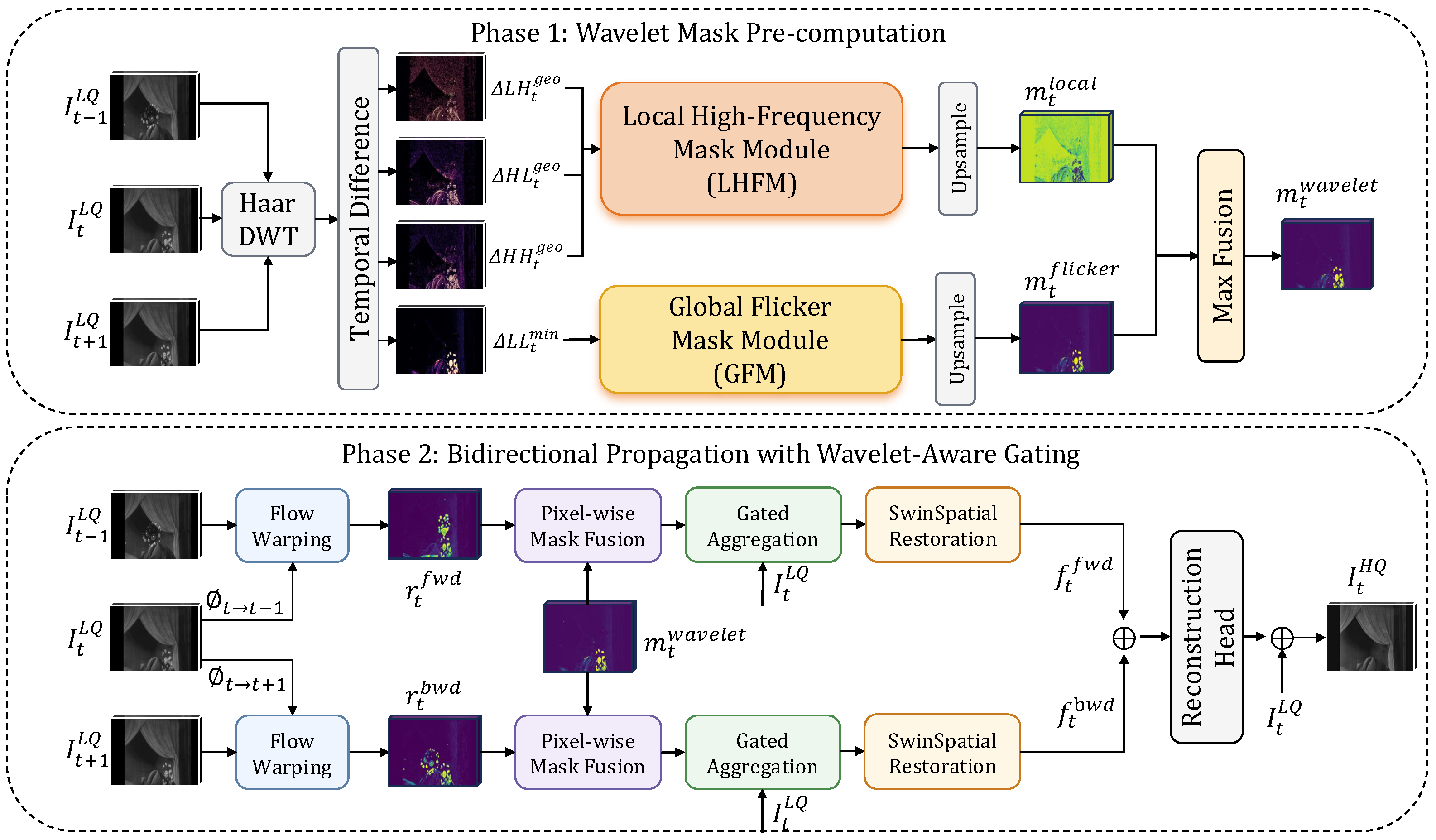
Figure 2 summarizes the final WaveletMask pipeline. For each frame, the WaveletNoiseMask block pre-computes a wavelet-domain gate mask from the current frame and its two temporal neighbors, and the resulting $m_t^{\mathrm{wavelet}}$ is injected directly into the forward and backward recurrent gates in Equation (2). The restoration backbone, bidirectional propagation schedule, and training losses remain identical to RTN; only the gate input is changed.

Unlike the flow-guided propagation path in RTN, the wavelet detector intentionally operates on raw temporal neighbors instead of motion-compensated ones. An auxiliary code path includes an optional flow-compensated wavelet variant, but this switch is disabled in the proposed model because a small pixel-domain misregistration perturbs multiple LL/LH/HL/HH coefficients after the discrete wavelet transform, thereby amplifying optical-flow errors into structured false responses near motion boundaries. For the same reason, the proposed model fixes a single-level Haar decomposition; alternative wavelet families and learned fusion variants are reserved for ablation-only experiments.

The recurrent aggregation step can be written as

$$f_t^{\mathrm{agg}}=\mathrm{GatedAgg}(f_{\mathrm{prop}},I_t^{\mathrm{LQ}},m_{t,d}^{\mathrm{gate}}),$$

(3)

where $m_{t,d}^{\mathrm{gate}}$ is broadcast along the feature-channel dimension. The reconstruction head follows the original RTN contract:

$$I_t^{\mathrm{HQ}}=tanh\left(\mathrm{Upsample}\right([f_t^{\mathrm{bwd}},f_t^{\mathrm{fwd}}])+I_t^{\mathrm{LQ}}).$$

(4)

Because the wavelet mask is pre-computed before recurrent propagation and the final fusion is parameter-free, the proposed variant changes only the gate input while leaving the restoration backbone, losses, and propagation structure unchanged.

Figure 2. Overview of the final WaveletMask pipeline. The WaveletNoiseMask module pre-computes the branch-max wavelet mask $m_t^{\mathrm{wavelet}}$ from neighboring frames, and the resulting mask is injected directly into the forward and backward recurrent gates. Learned CNN fusion variants that additionally use the RTN spatial indicator are ablated in Table A11 and are not part of the proposed model.

Figure 2. Overview of the final WaveletMask pipeline. The WaveletNoiseMask module pre-computes the branch-max wavelet mask $m_t^{\mathrm{wavelet}}$ from neighboring frames, and the resulting mask is injected directly into the forward and backward recurrent gates. Learned CNN fusion variants that additionally use the RTN spatial indicator are ablated in Table A11 and are not part of the proposed model.

3.3. Local High-Frequency Mask Module (LHFM)

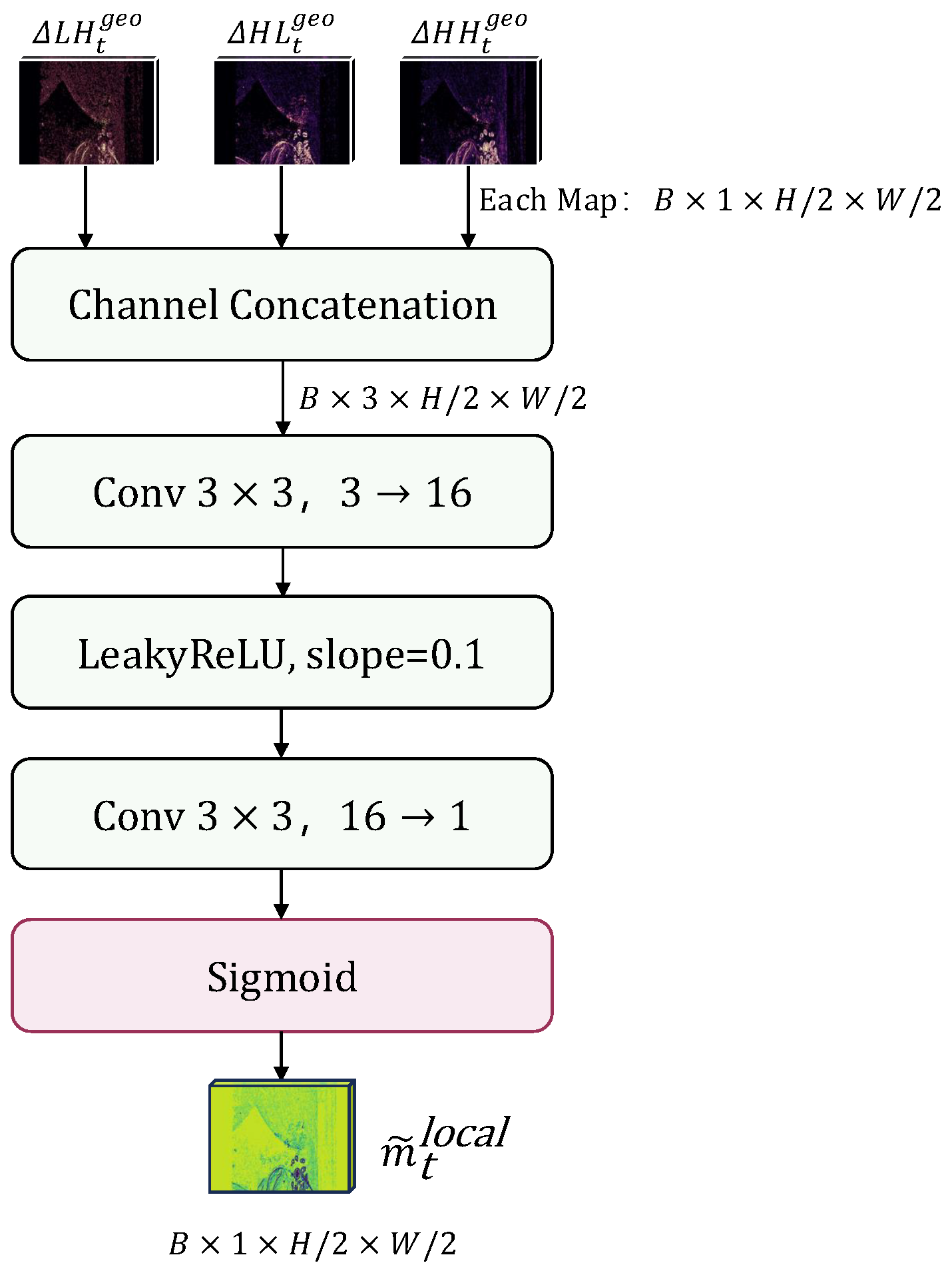
Unlike pixel-domain differences that entangle thin defects with motion boundaries and warping residuals, LHFM isolates transient local corruption by measuring bilateral consistency in the wavelet detail sub-bands. Figure 3 shows the module architecture.

Each RGB frame is first converted to luminance using the BT.601 transform, $I_t^{\mathrm{gray}}=0.299R+0.587G+0.114B$, and is then decomposed of a single-level Haar DWT:

$$\{{\mathrm{LL}}_t,{\mathrm{LH}}_t,{\mathrm{HL}}_t,{\mathrm{HH}}_t\}=\mathrm{HaarDWT}2\mathrm{d}\left(I_t^{\mathrm{gray}}\right).$$

(5)

Here, ${\mathrm{LL}}_t$ denotes the low-frequency approximation, while ${\mathrm{LH}}_t$, ${\mathrm{HL}}_t$, and ${\mathrm{HH}}_t$ denote the horizontal, vertical, and diagonal detail coefficients, respectively. The proposed model uses fixed $2\times 2$ Haar analysis filters normalized by $1/2$, so the transform introduces no learnable parameters.

To suppress one-sided temporal residuals, LHFM requires simultaneous disagreement with both temporal neighbors. For each high-frequency sub-band $S\in \{\mathrm{LH},\mathrm{HL},\mathrm{HH}\}$, the bilateral response is computed as

$$d_t^S=\sqrt{|S_t-S_{t^{-}}\left|\right|S_t-S_{t^{+}}|+ϵ},$$

(6)

where $t^{-}$ and $t^{+}$ denote the previous and next neighbors for non-boundary frames, and $ϵ={10}^{-8}$ is used for numerical stability. The geometric mean behaves like a bilateral “and” operator: if either temporal difference is small, the overall response remains small. Consequently, one-sided motion or warping residuals are attenuated, whereas a transient scratch or dust particle that differs from both neighbors produces a strong activation. Boundary frames do not have bilateral temporal evidence and are assigned zero wavelet masks. This design is effective for single-frame defects, but when a scratch persists across three or more consecutive frames at nearly the same image-plane position ($S_{t-1}\approx S_t\approx S_{t+1}$), both temporal differences vanish and $d_t^S\to 0$, suppressing the LHFM response (see Section 3.6 and

Table A7. Detector response to controlled persistent scratches. Relative response is normalized by the same mode’s single-frame ($L=1$) response. Suppression is $1-\mathrm{relative}$ for the raw LHFM response.

Mode	L	Clips	Raw LHFM	Raw Relative Response	Raw Suppression	${\mathit{m}}_{\mathbf{wavelet}}$ Relative Response
Fixed	1	12	0.0862	1.0000	0.0000	1.0000
Fixed	2	12	0.0462	0.5355	0.4645	0.0167
Fixed	3	12	0.0302	0.3498	0.6502	0.0108
Fixed	5	12	0.0302	0.3498	0.6502	0.0108
Drift	1	12	0.0862	1.0000	0.0000	1.0000
Drift	2	12	0.0894	1.0364	−0.0364	0.1363
Drift	3	12	0.0957	1.1097	−0.1097	0.0419
Drift	5	12	0.0957	1.1097	−0.1097	0.0419

).

Figure 3. LHFM architecture. Geometric-mean temporal differences from the LH, HL, and HH detail sub-bands are concatenated and processed by high_freq_conv, consisting of a 3 × 3 3→16 convolution, LeakyReLU, a 3 × 3 16→1 convolution, and sigmoid activation. The half-resolution output ${\tilde{m}}_t^{\mathrm{local}}\in {[0,1]}^{1\times H/2\times W/2}$ is bilinearly upsampled before fusion.

Figure 3. LHFM architecture. Geometric-mean temporal differences from the LH, HL, and HH detail sub-bands are concatenated and processed by high_freq_conv, consisting of a 3 × 3 3→16 convolution, LeakyReLU, a 3 × 3 16→1 convolution, and sigmoid activation. The half-resolution output ${\tilde{m}}_t^{\mathrm{local}}\in {[0,1]}^{1\times H/2\times W/2}$ is bilinearly upsampled before fusion.

The three directional responses are then aggregated by a lightweight prediction head:

$${\tilde{m}}_t^{\mathrm{local}}=\sigma \left({\mathrm{Conv}}_{16\to 1}\right(\mathrm{LeakyReLU}\left({\mathrm{Conv}}_{3\to 16}\right([d_t^{\mathrm{LH}},d_t^{\mathrm{HL}},d_t^{\mathrm{HH}}]\left)\right)\left)\right),$$

(7)

where $\sigma$ denotes the sigmoid activation and $[·]$ denotes channel-wise concatenation. The resulting half-resolution prediction is bilinearly upsampled to the image resolution:

$$m_t^{\mathrm{local}}=\mathrm{Up}\left({\tilde{m}}_t^{\mathrm{local}}\right), m_t^{\mathrm{local}}\in {[0,1]}^{1\times H\times W},$$

(8)

where $\mathrm{Up}(·)$ denotes bilinear upsampling.

3.4. Global Flicker Mask Module (GFM)

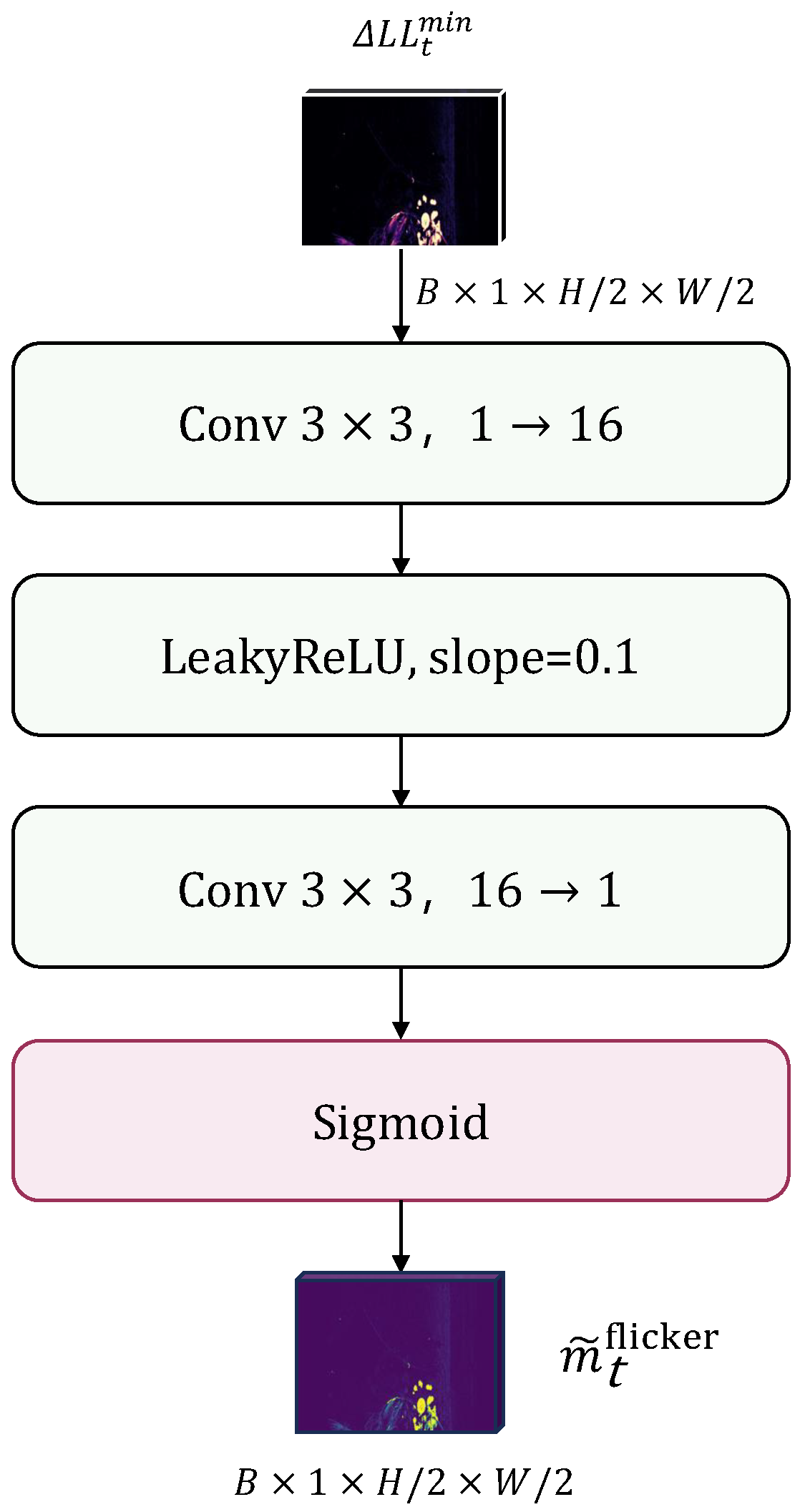
Unlike pixel-domain differences that are dominated by edges, texture, and local motion, GFM captures frame-level photometric instability by measuring bilateral low-frequency deviations on the LL sub-band. Figure 4 shows the module architecture.

After obtaining the LL coefficients, we compute the forward and backward low-frequency deviations as

$$d_t^{\mathrm{fwd}}=|{\mathrm{LL}}_t-{\mathrm{LL}}_{t^{-}}|, d_t^{\mathrm{bwd}}=|{\mathrm{LL}}_t-{\mathrm{LL}}_{t^{+}}|.$$

(9)

GFM then enforces bilateral agreement through a minimum operator:

$$d_t^{\mathrm{flicker}}=min(d_t^{\mathrm{fwd}},d_t^{\mathrm{bwd}}).$$

(10)

The minimum rule is used instead of an average because a genuine flicker event should increase both forward and backward LL differences. If only one direction is large, the response is limited to the smaller value, which reduces sensitivity to one-sided brightness changes. At the same time, abrupt scene cuts, flashes, and other broad illumination changes can also elevate both LL differences. These failure modes are quantified in

Table A6. GFM response on synthetic failure-mode probes. Activation is the mean GFM mask value on non-boundary frames. Ratio compares probe activation with the corresponding clean clip. Suppression reports the activation reduction after a simple luminance-difference cut guard, which is evaluated post hoc and is not part of the deployed WaveletMask model.

Probe	Clips	Clean Activation	Probe Activation	Ratio	FPR	Guarded Activation	Suppression
Scene cut	12	0.0041	0.0066	2.35×	0.0505	0.0024	0.6141
Exposure flash	12	0.0041	0.0257	10.41×	0.1574	0.0015	0.9470
Illumination ramp	12	0.0041	0.0051	1.52×	0.0352	0.0049	0.0247

and discussed in Section 3.6.

Figure 4. GFM architecture. The minimum LL temporal response is processed by low_freq_conv, consisting of a 3 × 3 1→16 convolution, LeakyReLU, a 3 × 3 16→1 convolution, and sigmoid activation. The half-resolution output ${\tilde{m}}_t^{\mathrm{flicker}}\in {[0,1]}^{1\times H/2\times W/2}$ is bilinearly upsampled before fusion.

Figure 4. GFM architecture. The minimum LL temporal response is processed by low_freq_conv, consisting of a 3 × 3 1→16 convolution, LeakyReLU, a 3 × 3 16→1 convolution, and sigmoid activation. The half-resolution output ${\tilde{m}}_t^{\mathrm{flicker}}\in {[0,1]}^{1\times H/2\times W/2}$ is bilinearly upsampled before fusion.

The low-frequency response is decoded by a second lightweight prediction head:

$${\tilde{m}}_t^{\mathrm{flicker}}=\sigma \left({\mathrm{Conv}}_{16\to 1}\right(\mathrm{LeakyReLU}\left({\mathrm{Conv}}_{1\to 16}\left(d_t^{\mathrm{flicker}}\right)\right)\left)\right),$$

(11)

followed by bilinear upsampling to the original resolution:

$$m_t^{\mathrm{flicker}}=\mathrm{Up}\left({\tilde{m}}_t^{\mathrm{flicker}}\right), m_t^{\mathrm{flicker}}\in {[0,1]}^{1\times H\times W}.$$

(12)

3.5. Mask Fusion and Integration

Unlike pixel-domain differences that collapse local scratches and global luminance shifts into a single motion-sensitive residual, the integration stage preserves whichever wavelet branch provides the stronger evidence at each pixel. As further clarified in Section 3.6, LHFM and GFM are complementary rather than redundant, so the fusion rule should avoid attenuating a decisive single-branch response.

WaveletMask therefore uses a branch-level maximum operation:

$$m_t^{\mathrm{wavelet}}=max(m_t^{\mathrm{local}},m_t^{\mathrm{flicker}}).$$

(13)

The element-wise maximum treats local structural damage and global flicker as alternative degradation evidence: if either branch fires, the wavelet mask is activated. This choice also matches the implementation exactly, where $max(·,·)$ is used directly after the two mask heads. Compared with learned convex fusion, this rule preserves a strong activation from either branch instead of averaging it with a weak companion response. The ablation results in Table A11 further show that parameter-free max fusion is preferable to learned PixelWiseMaskFusion, which supports the final design choice.

The complete detector consists of the fixed Haar DWT and two lightweight CNN heads, introducing only 898 learnable detector parameters. By contrast, the learned PixelWiseMaskFusion ablation adds 14,497 additional fusion parameters and also mixes in the RTN spatial indicator. These learned spatial–wavelet fusion variants are therefore treated as ablations rather than components of the final WaveletMask model.

3.6. Response Analysis

To clarify the design rationale and boundary conditions of LHFM and GFM, we analyze several canonical temporal patterns.

Local high-frequency response. Equation (6) is designed to respond strongly only when the current high-frequency coefficient differs from both temporal neighbors. For a single-frame transient scratch at time t ($S_{t-1}=0,S_t>0,S_{t+1}=0$), both terms under the geometric mean are large, producing the intended strong $d_t^S$ response. If only one directional difference is elevated, the product remains limited, which explains why the geometric mean suppresses one-sided motion or warping residuals more effectively than a simple sum or average. Conversely, for a persistent fixed scratch spanning ≥3 frames ($S_{t-1}\approx S_t\approx S_{t+1}$), both temporal differences vanish and $d_t^S\to 0$, suppressing the LHFM response. This is an inherent boundary condition of the bilateral design: persistent image-plane-fixed scratches are progressively attenuated with increasing persistence length (46% suppression at $L=2$, 65% at $L\ge 3$; see Table A7). Drifting scratches that shift spatially between frames break the equality condition and are therefore not suppressed in the same way.

Global flicker response. Equation (10) similarly enforces bilateral agreement, but on the low-frequency LL component. A valid flicker event causes both forward and backward LL differences to increase, so the minimum remains high; this is why the minimum rule is better aligned with frame-level flicker than an average that can be dominated by a single-sided deviation. However, scene cuts and exposure flashes also produce bilateral LL elevation. In our probes, a scene cut yields $2.35\times$ baseline activation, and a flash yields $10.41\times$ (Table A6). A luminance-difference guard can suppress 61% of scene-cut and 95% of flash false responses, but it is not integrated into the current model in order to keep the proposed detector lightweight and scope-consistent.

Taken together, these complementary response patterns explain the integration strategy in Section 3.5: the final gate should preserve the stronger local or global cue at each pixel, rather than learn an averaging rule that may dilute a decisive single-branch response.

3.7. Training Objective

Training follows the RTN protocol [3]. The total objective is

$${\mathcal{L}}_{\mathrm{total}}={\mathcal{L}}_{\mathrm{pix}}+{\lambda }_{\mathrm{perc}}{\mathcal{L}}_{\mathrm{perc}}+{\lambda }_{\mathrm{gan}}{\mathcal{L}}_{\mathrm{gan}},$$

(14)

where ${\mathcal{L}}_{\mathrm{pix}}$ is an $L_1$ reconstruction loss, ${\mathcal{L}}_{\mathrm{perc}}$ is a VGG-based perceptual loss [37,38], and ${\mathcal{L}}_{\mathrm{gan}}$ is a non-saturating adversarial loss [39]. The weights are ${\lambda }_{\mathrm{perc}}=1.0$ and ${\lambda }_{\mathrm{gan}}=0.01$, following RTN [3]. No explicit mask supervision is used; the wavelet branches and the restoration backbone are optimized only through the restoration losses. This choice preserves compatibility with the baseline training loop, but it also limits how strongly the learned masks can be interpreted as ground-truth artifact segmentations.

4. Experiments

This section describes the experimental setup, compares WaveletMask with state-of-the-art methods on synthetic and real-world data, presents the ablation study, and analyzes computational complexity. Detailed statistical-reliability analyses, robustness and cross-content generalization studies, detector diagnostic probes, and full ablation sweeps are reported in Appendix A, Appendix B, Appendix C and Appendix D.

4.1. Datasets

Experiments were conducted on the Synthetic and Real-World Old Video (SRWOV) benchmark introduced with MambaOFR [8]. The synthetic split provides paired ground truth and is used for full-reference evaluation. The real-world split contains archival clips without paired ground truth and is used for no-reference metrics and qualitative comparisons.

Training used the REDS training split [40]. Clean REDS frames were degraded on the fly with the synthetic film degradation pipeline used by RTN [3], including scratches, dust, blotches, flicker, and grain. The SRWOV synthetic test set contains 30 clips rendered from held-out REDS sequences, and the SRWOV real-world set contains 216 archival clips. Unless otherwise noted, the quantitative results below are reported within this SRWOV protocol. Qualitative figures are illustrative; statistical claims rest on the unified re-training benchmark in

Table 3. Unified re-training benchmark on the SRWOV synthetic split (30 clips, Y-channel protocol), listed in chronological order of publication with the proposed WaveletMask in the last row. All methods, including WaveletMask, were re-trained and re-evaluated by us under one unified benchmark pipeline, so the rows are directly comparable. Best results are in red and second-best results in blue. Bold denotes the proposed method. Upward arrows indicate metrics for which higher values are better, and downward arrows indicate metrics for which lower values are better.

Method	Year	PSNR ↑	SSIM ↑	LPIPS ↓	DISTS ↓
DeepRemaster [2]	2019	25.0590	0.9185	0.1108	0.0895
DeOldify [41]	2019	23.2197	0.8923	0.2775	0.1260
OldPhoto [4]	2020	24.6174	0.8524	0.2252	0.1144
RTN [3]	2022	25.8514	0.8869	0.1214	0.0862
RVRT [23]	2022	22.4317	0.8710	0.1655	0.1078
ShiftNet [25]	2023	21.4817	0.8234	0.2030	0.1303
RRTN [7]	2024	24.1450	0.9006	0.1082	0.0668
VRT [24]	2024	22.3866	0.8631	0.1750	0.1087
MambaOFR [8]	2025	25.9938	0.9059	0.0815	0.0822
WaveletMask (ours)	2026	26.6017	0.8951	0.0891	0.0831

and the strict paired controlled analysis in Appendix A.

4.2. Implementation Details

RTN and all WaveletMask variants are trained with the same recipe. We use Adam [42] with ${\beta }_1=0.9$, ${\beta }_2=0.99$, initial learning rate $2\times {10}^{-4}$, and a MultiStep schedule with milestones at 50K, 100K, and 150K iterations. Training uses 200K iterations, seven input frames, $256\times 256$ crops, and batch size 1 per GPU. The configuration sets fix_flow_iters = 0.0005, so the RAFT [20] optical-flow estimator is effectively trained jointly from the start rather than frozen for a 500-iteration warm-up. Experiments are implemented in PyTorch with the BasicSR toolbox [43]; inference is performed at full resolution. The strict paired controlled comparison against the RTN (Appendix A) is reported for seed 2021, and a three-seed Y-channel re-test is reported separately to assess seed stability.

4.3. Evaluation Metrics

Following common practice in old-film restoration [3,7,8], we adopt three complementary groups of metrics. (1) On the synthetic split with paired ground truth, we report the fidelity metrics PSNR and SSIM [44] together with the perceptual metrics LPIPS [45] and DISTS [46]; all full-reference metrics are computed under the Y-channel protocol. (2) On the real-world split without ground truth, we report the no-reference metrics NIQE [47], BRISQUE [48], and CLIPIQA+ [49]; these no-reference metrics, together with the qualitative comparisons, constitute the primary real-world evidence. (3) To quantify statistical reliability, we report clip-level bootstrap confidence intervals, two-sided paired permutation tests, and a three-seed re-test for the paired controlled comparison; the complete statistics are provided in Appendix A.

For completeness, the two primary full-reference metrics are defined as follows. Given a restored luminance frame $\widehat{I}$ and its ground truth I with N pixels, the peak signal-to-noise ratio (PSNR) is

$$\mathrm{PSNR}(\widehat{I},I)=10{log}_{10}{\displaystyle \frac{L^2}{\frac{1}{N}{\sum }_{i=1}^N{({\widehat{I}}_i-I_i)}^2}},$$

(15)

where L is the maximum possible pixel value, and the structural similarity index (SSIM) is

$$\mathrm{SSIM}(\widehat{I},I)={\displaystyle \frac{(2{\mu }_{\widehat{I}}{\mu }_I+c_1)(2{\sigma }_{\widehat{I}I}+c_2)}{({\mu }_{\widehat{I}}^2+{\mu }_I^2+c_1)({\sigma }_{\widehat{I}}^2+{\sigma }_I^2+c_2)}},$$

(16)

where ${\mu }_{·}$ and ${\sigma }_{·}$ denote local means and standard deviations; ${\sigma }_{\widehat{I}I}$ is the local covariance; and $c_1,c_2$ are small stabilizing constants. The perceptual metrics LPIPS and DISTS and the no-reference metrics NIQE, BRISQUE, and CLIPIQA+ follow the definitions in their original references.

4.4. Comparison with State-of-the-Art Methods

We compare WaveletMask with representative methods from three categories: old photo restoration applied per frame (OldPhoto [4] and DeOldify [41]); general video restoration (ShiftNet [25], VRT [24], and RVRT [23]); and dedicated old-film restoration (DeepRemaster [2], RTN [3], RRTN [7], and MambaOFR [8]). All ten methods, including WaveletMask, were re-trained and re-evaluated on the same SRWOV synthetic split under one unified benchmark pipeline, so they are directly comparable; in addition, a strict paired controlled analysis against RTN—which shares the backbone, training data, degradation pipeline, and metric scripts with WaveletMask—is reported in Appendix A.

4.4.1. Quantitative Comparison on Synthetic Data

Table 3 reports the unified re-training benchmark over ten methods. Under this single comparable protocol, WaveletMask attains the best PSNR (26.60 dB, $+0.61$ dB over the strongest competitor MambaOFR) and the second-best LPIPS. On DISTS it is essentially tied with the second-best method (0.0831 vs. 0.0822 for MambaOFR), whereas on SSIM it sits mid-table, behind the perception-oriented methods DeepRemaster, MambaOFR, and RRTN. The benchmark thus indicates a clear fidelity advantage, together with competitive perceptual quality, rather than uniform dominance across metrics: among the recent dedicated baselines, MambaOFR remains the strongest on the structural and perceptual scores, while WaveletMask leads on PSNR at a fraction of the detector parameter cost (Section 4.6). Beyond this benchmark, a strict paired controlled comparison against the RTN isolates the contribution of the proposed gate: WaveletMask improves PSNR by $+0.45$ dB, all four paired clip-level gains are statistically significant under two-sided permutation tests ($p\le 1.5\times {10}^{-3}$), and a three-seed re-test confirms that the advantage persists with markedly higher stability than the baseline (26.22 ± 0.37 vs. 24.56 ± 1.67 dB PSNR; Appendix A,

Table A1. Paired controlled comparison on the SRWOV synthetic benchmark (seed 2021, Y-channel protocol, 30 clips). RTN and WaveletMask share the same data, degradation pipeline, implementation, and metric scripts, so this strict paired comparison is the controlled evidence for the proposed gate. The paired improvement reports WaveletMask minus RTN for PSNR/SSIM and RTN minus WaveletMask for LPIPS/DISTS (positive favors WaveletMask); confidence intervals use clip-level bootstrap resampling and p-values use a two-sided paired permutation test. The WaveletMask paired-protocol PSNR (26.6125 dB) differs slightly from the unified-benchmark value in Table 3 (26.6017 dB) because the two protocols use different training checkpoints and metric configurations. Best values in each row are in red.

Metric	RTN	WaveletMask	Paired Improvement	95% CI/Two-Sided p
PSNR ↑	26.1648	26.6125	$+0.4477$	$[0.2955,0.5981]$, $p=5\times {10}^{-5}$
SSIM ↑	0.8923	0.8954	$+0.0031$	$[0.0014,0.0050]$, $p=1.5\times {10}^{-3}$
LPIPS ↓	0.1023	0.0886	$+0.0137$	$[0.0108,0.0166]$, $p=5\times {10}^{-5}$
DISTS ↓	0.0946	0.0827	$+0.0119$	$[0.0103,0.0136]$, $p=5\times {10}^{-5}$

and

Table A2. Three-seed same-protocol Y-channel re-test on the SRWOV synthetic benchmark. Values are mean ± standard deviation over seeds 2021, 2022, and 2023. Best results are in red. Bold denotes the proposed method.

Method	PSNR ↑	SSIM ↑	LPIPS ↓	DISTS ↓
RTN [3]	24.5570 ± 1.6667	0.8808 ± 0.0129	0.1083 ± 0.0118	0.0922 ± 0.0040
WaveletMask (ours)	26.2183 ± 0.3725	0.8983 ± 0.0045	0.0879 ± 0.0026	0.0831 ± 0.0015
Mean difference	+1.6613	+0.0175	−0.0205	−0.0091

). The WaveletMask unified-benchmark entry (26.6017 dB) differs slightly from this paired value (26.6125 dB), and the unified-benchmark RTN entry (25.8514 dB) likewise differs from the paired-protocol RTN (26.1648 dB in the ablation study), because the two protocols use different training checkpoints and metric configurations. The gain is not confined to a single degradation mode: it is positive in all artifact-dominant strata, remains stable across motion and occlusion terciles, and transfers to unseen DAVIS content in PSNR, LPIPS, and DISTS under the same degradation pipeline (Appendix B).

4.4.2. No-Reference Comparison on Real-World Data

Real-world SRWOV clips do not have paired ground truth, so we report them separately from the full-reference synthetic results.

Table 4. No-reference evaluation on the 216-clip SRWOV real-world split. All values are measured by us under the unified benchmark pipeline; the degraded-input row is the unrestored anchor scored with the same per-frame protocol. Best results among the restoration methods are in red and second-best in blue; the degraded-input anchor is excluded from the ranking. Bold denotes the proposed method.

Method	NIQE ↓	BRISQUE ↓	CLIPIQA+ ↑
Degraded input	5.7745	43.1050	0.3873
DeOldify [41]	5.7218	41.6118	0.3768
DeepRemaster [2]	5.9917	40.6158	0.3991
OldPhoto [4]	6.5601	30.4532	0.4503
RTN [3]	5.1723	19.0031	0.4163
VRT [24]	5.6551	42.7296	0.3985
RVRT [23]	5.7217	42.6402	0.4013
ShiftNet [25]	5.7126	42.8195	0.3975
RRTN [7]	5.6664	32.8572	0.3969
MambaOFR [8]	5.3381	29.7853	0.4351
WaveletMask (ours)	5.2288	24.2023	0.4356

reports our unified-benchmark no-reference scores for all ten methods, together with the degraded-input anchor on the 216-clip SRWOV real-world split. A no-reference ablation over the RTN/LHFM/GFM variants under the strict paired protocol (Appendix A) is provided in Appendix D (

Table A14. No-reference ablation of the RTN/LHFM/GFM variants on the 216-clip SRWOV real-world split, measured under the strict paired protocol (Appendix A). Checkmarks indicate included branches, and dashes indicate absent branches. Lower NIQE/BRISQUE indicates better statistical naturalness; higher CLIPIQA+ indicates better CLIP-based perceptual quality. The best result within this ablation is in red.

Variant	LHFM	GFM	NIQE ↓	BRISQUE ↓	CLIPIQA+ ↑
RTN	—	—	5.3340	29.3119	0.4359
+LHFM only	✓	—	5.3392	19.5562	0.4115
+GFM only	—	✓	5.0400	28.7878	0.4388
WaveletMask	✓	✓	5.2288	24.2023	0.4356

).

In Table 4, the ranking is mixed across NIQE, BRISQUE, and CLIPIQA+, which is expected for content-dependent no-reference metrics: the RTN checkpoint attains the best NIQE and BRISQUE; OldPhoto attains the best CLIPIQA+; and WaveletMask ranks second on all three metrics—the only method placing within the top two on every no-reference dimension, although its CLIPIQA+ margin over MambaOFR is narrow (0.4356 vs. 0.4351). Restoration clearly improves NIQE and BRISQUE over the degraded-input anchor for the strongest methods, yet individual no-reference metrics disagree on the absolute ranking, and the scores are sensitive to the training checkpoint: the paired-protocol RTN checkpoint in Appendix D (Table A14) receives a clearly different BRISQUE score. The no-reference scores are therefore interpreted jointly with the qualitative comparisons below rather than as a standalone ranking. As an additional perceptual assessment on the real-world clips, an expert-level subjective evaluation is reported in the Supplementary Materials (Tables S1 and S2 and Figure S4).

4.4.3. Qualitative Comparison

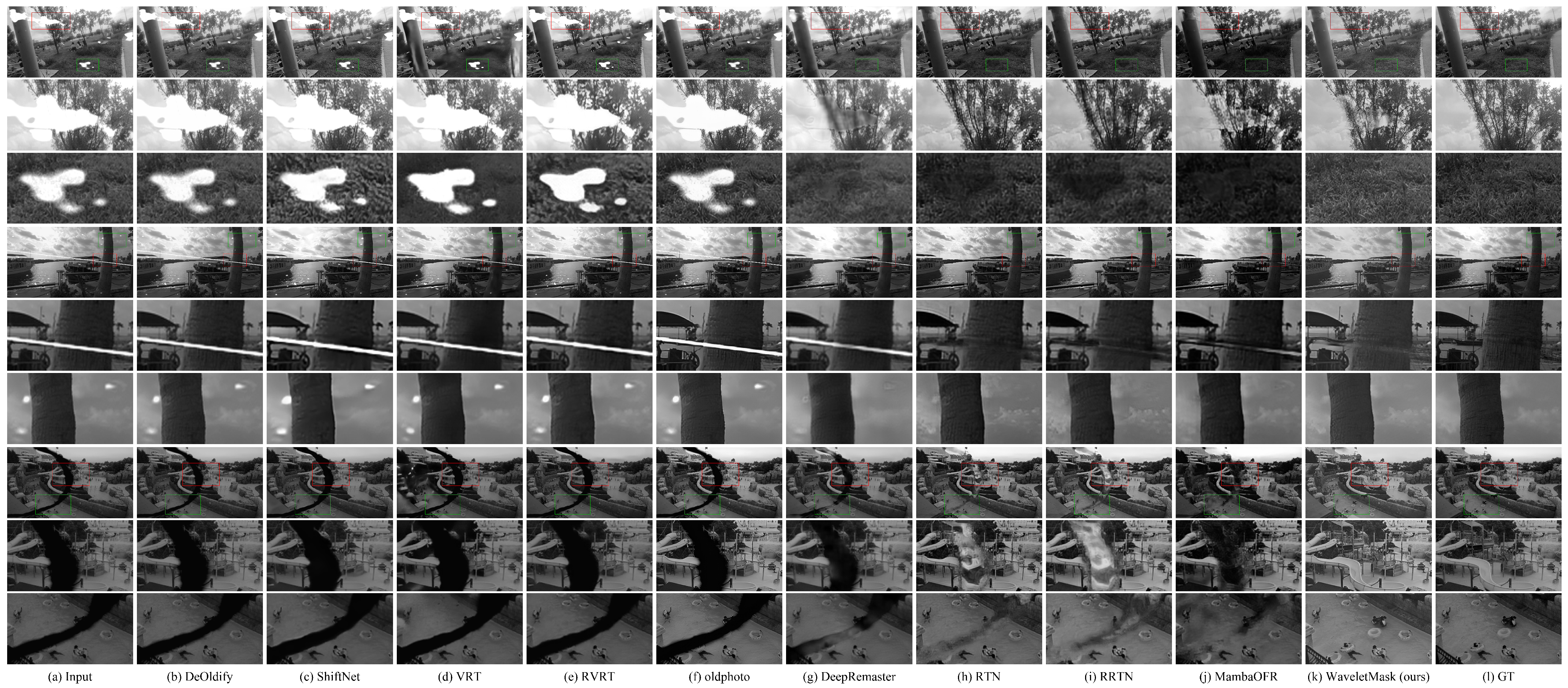
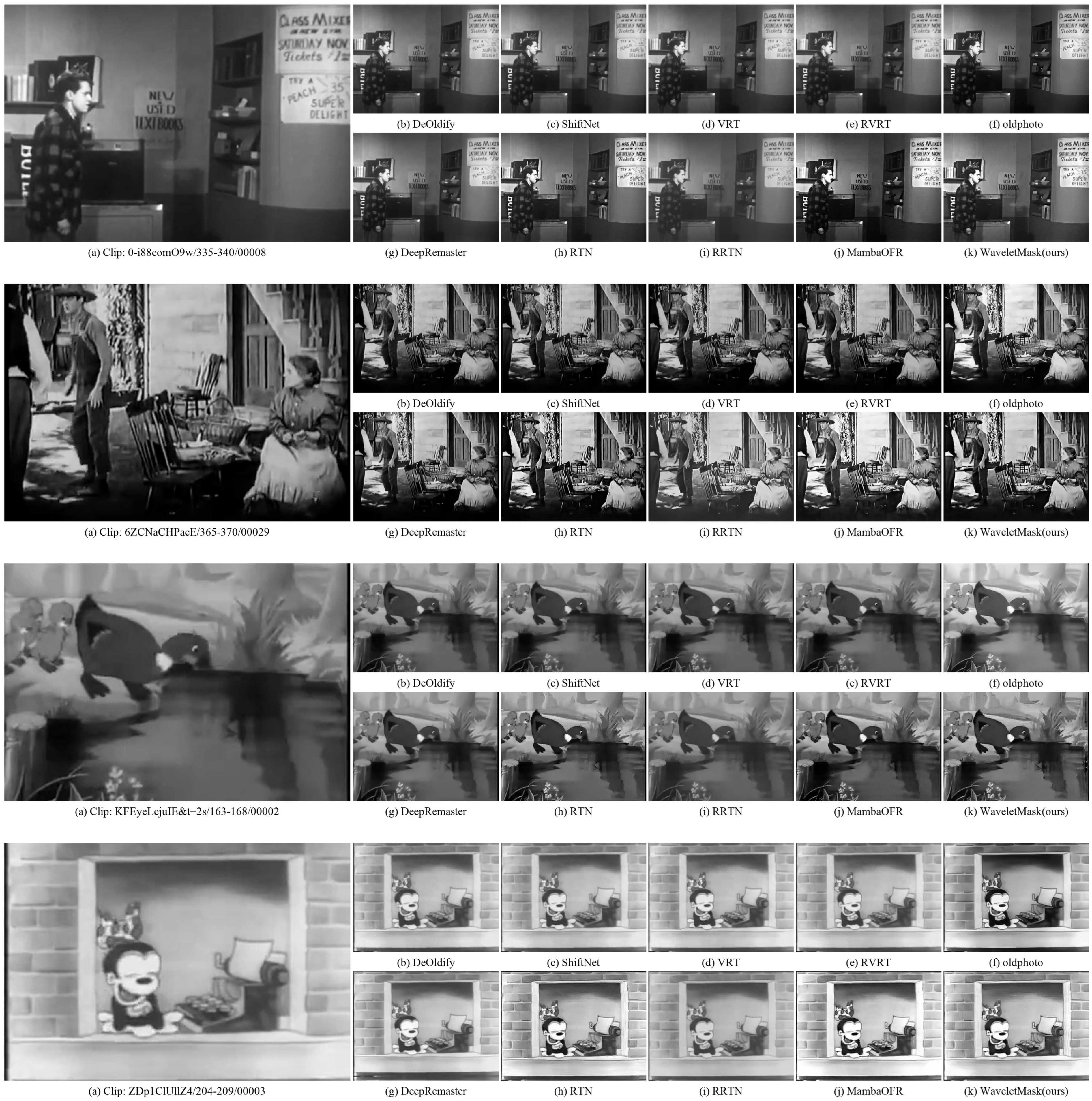
Figure 5 shows representative synthetic examples, where WaveletMask removes scratch and dust residuals more cleanly than the RTN output in the highlighted ROIs. Figure 6 shows the same tendency on archival clips, with cleaner local damage removal and more stable brightness restoration while preserving scene appearance. Spatial-error-map analysis confirms that the gains are concentrated in damaged regions (Supplementary Figure S5). The overall improvement raises the question of whether the gain is uniform across degradation types, which is analyzed in Appendix B.1.

4.5. Ablation Study

The ablation study is organized around four questions:

• Q1 (branch effectiveness). Do LHFM and GFM each improve over the RTN pixel-domain gate, and are the two branches complementary?
• Q2 (fusion rule). Is parameter-free branch-level maximum fusion preferable to learned pixel-wise fusion?
• Q3 (wavelet family). How sensitive is the gate to the wavelet basis and the number of decomposition levels?
• Q4 (robustness). Do the gains persist across artifact types, motion and occlusion levels, and unseen content (Appendix B)?

Q1–Q3 are addressed by the three panels of

Table 5. Ablation study on SRWOV synthetic data: panel (a) compares the detection-branch components; panel (b) the proposed branch-level maximum rule against representative learned-fusion variants; and panel (c) representative wavelet families. All variants share the same RTN backbone and training recipe. Within panel (a), best results are in red and second-best results in blue. Italic sub-headers denote the three ablation panels (a)–(c), and bold denotes the proposed WaveletMask configuration. Upward arrows indicate metrics for which higher values are better, and downward arrows indicate metrics for which lower values are better.

Variant	PSNR ↑	SSIM ↑	LPIPS ↓	DISTS ↓
(a) Detection-branch components
RTN	26.1648	0.8923	0.1023	0.0946
+LHFM only	26.3778	0.8966	0.0914	0.0790
+GFM only	26.1024	0.8980	0.0969	0.0916
WaveletMask (max fusion)	26.6125	0.8954	0.0886	0.0827
(b) Fusion strategy (key contrasts)
Branch-level maximum (proposed)	26.6125	0.8954	0.0886	0.0827
Gated CNN fusion	26.3515	0.8966	0.0869	0.0842
Max + pixel-wise CNN fusion	24.9827	0.8896	0.1068	0.0867
(c) Wavelet family (key contrasts)
Haar, single level (proposed)	26.6125	0.8954	0.0886	0.0827
Haar, two levels	26.5175	0.9011	0.0847	0.0760
DTCWT (dual-tree complex)	26.4506	0.8992	0.0862	0.0780
Daubechies-2	17.9208	0.6473	0.4136	0.3154

, while Q4 is examined in Appendix B. To isolate the contribution of the wavelet-domain branches and the key design choices, Table 5 groups three sets of contrasts under the same RTN backbone and training recipe: (a) the detection-branch components (RTN, +LHFM-only, +GFM-only, and the full WaveletMask variant with branch-level maximum fusion as defined in Equation (13)); (b) the key fusion-strategy contrasts between the parameter-free maximum rule and learned CNN fusion; and (c) the key wavelet-family contrasts around the single-level Haar default. The RTN, WaveletMask, and panel (c) rows are measured under the primary Y-channel re-test, whereas the +LHFM-only, +GFM-only, and learned-fusion rows come from an earlier identical-recipe evaluation run with a slightly different LPIPS/DISTS configuration; the cross-run drift is below 0.002 on these two metrics and does not affect the within-panel ranking.

Panel (a) of Table 5 shows that LHFM alone improves PSNR by $+0.21$ dB over the RTN and yields the lowest DISTS, confirming the value of high-frequency local cues. GFM alone slightly reduces PSNR ($-0.06$ dB) but achieves the best SSIM, indicating stronger structural consistency. The full WaveletMask model reaches 26.61 dB, a $+0.45$ dB gain over RTN, and the best LPIPS among the four variants. This is because LHFM targets local scratches and dust, whereas GFM stabilizes low-frequency temporal brightness variation, so their fusion provides complementary guidance. The combined improvement is larger than the arithmetic sum of the individual PSNR changes ($+0.21-0.06=+0.15$ dB), which further supports the complementarity of the two branches.

Figure 6. Qualitativecomparison on SRWOV real-world archival clips without paired ground truth. Each row compares one input clip/ROI with outputs from (a) input, (b) DeOldify, (c) ShiftNet, (d) VRT, (e) RVRT, (f) OldPhoto, (g) DeepRemaster, (h) RTN, (i) RRTN, (j) MambaOFR, and (k) WaveletMask. Full-reference scores are unavailable for this split; repeated method-column labels denote the same method order across rows.

Figure 6. Qualitativecomparison on SRWOV real-world archival clips without paired ground truth. Each row compares one input clip/ROI with outputs from (a) input, (b) DeOldify, (c) ShiftNet, (d) VRT, (e) RVRT, (f) OldPhoto, (g) DeepRemaster, (h) RTN, (i) RRTN, (j) MambaOFR, and (k) WaveletMask. Full-reference scores are unavailable for this split; repeated method-column labels denote the same method order across rows.

Panel (b) condenses the fusion-strategy finding: every learned-fusion variant underperforms its direct counterpart in PSNR under the tested recipe (within the fusion-ablation evaluation run, the gated CNN variant trails the maximum rule by 0.25 dB and the max + CNN variant by 1.62 dB), because the compact CNN must fuse heterogeneous sparse cues only through the final restoration loss, making optimization less stable than the parameter-free maximum rule. The gated variant does attain slightly better SSIM and LPIPS than the maximum rule, but it remains behind on PSNR and DISTS, whereas the max + CNN variant is inferior on all four metrics; the parameter-free rule therefore remains the preferred default for the fidelity-oriented design goal. Panel (c) condenses the wavelet-family finding: single-level Haar is the most stable PSNR-oriented default, Haar two-level and DTCWT remain competitive with small PSNR costs and partial perceptual gains, and longer-support wavelets fail catastrophically because filter lengths exceeding two require boundary padding in the wavelet analysis, which introduces border artifacts into the half-resolution sub-band maps processed by the detector heads. The complete fusion comparison, the full wavelet-family and stronger-fusion sweeps, and a cross-domain frequency-operator diagnostic that situates Haar among Sobel/Laplacian, Gaussian-pyramid, Fourier-temporal, and learned shallow alternatives are reported in Appendix D (Table A11 and

Table A12. Extended ablation of wavelet families and stronger fusion alternatives under the Y-channel protocol. The proposed configuration is single-level Haar with branch-level maximum fusion.

Variant	PSNR ↑	SSIM ↑	LPIPS ↓	DISTS ↓
Haar, single level (seed 2021)	26.6125	0.8954	0.0886	0.0827
Haar, two levels	26.5175	0.9011	0.0847	0.0760
DTCWT (dual-tree complex)	26.4506	0.8992	0.0862	0.0780
Coiflet-1	25.8533	0.8874	0.1026	0.0893
Symlet-2	24.2087	0.8509	0.1507	0.1226
Daubechies-2	17.9208	0.6473	0.4136	0.3154
Attention fusion	23.2479	0.8281	0.1768	0.1359
Residual fusion	25.9777	0.8929	0.0966	0.0811

) and Appendix C (

Table A10. Cross-domain frequency-operator diagnostic on SRWOV/REDS residual proxies. Top-5 non-proxy reports the fraction of top-5% response pixels outside the residual-proxy region; lower is better. AUPRC is the primary ranking metric because several deterministic operators reach their best F1 only at a near-all-positive threshold. Learned shallow values report the five-fold mean.

Operator	Family	AUPRC ↑	Top-5 Hit ↑	Top-5 Non-Proxy ↓
Haar fused	Haar DWT	0.3166	0.3685	0.6315
Sobel	Gradient edge	0.3062	0.3470	0.6530
Laplacian	Gradient edge	0.2993	0.3352	0.6648
Gaussian fused	Gaussian pyramid	0.3270	0.3815	0.6185
Fourier temporal fused	Fourier temporal	0.3885	0.4384	0.5616
Learned shallow frequency	Proxy-supervised	0.4265	0.5278	0.4722

).

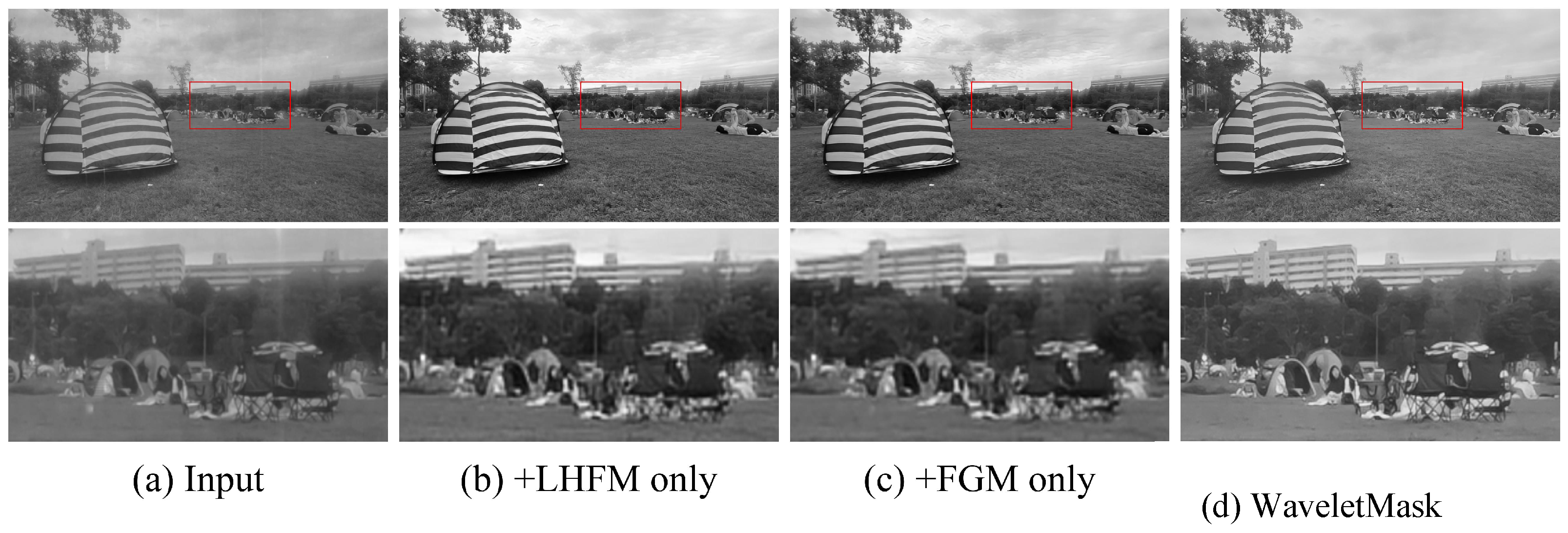
Figure 7 visually supports the same trend: LHFM mainly removes local scratches, GFM mainly stabilizes frame-level brightness, and the full model combines both effects. Beyond these end-to-end ablations, four detector diagnostic probes confirm that the two branches are complementary rather than redundant and that the fused mask aligns with residual-proxy regions (Appendix C).

4.6. Computational Complexity

Table 6. Computational cost measured by us under one unified protocol on a single NVIDIA L40 GPU (NVIDIA Corporation, Santa Clara, CA, USA) in FP32 (batch size 1, seven-frame $256\times 256$ clips, three warm-up and ten timed runs). Parameters and FLOPs cover the full executable forward pass on a $1\times 7\times 3\times 256\times 256$ input and include the RAFT flow estimator for the flow-based methods (RTN, RRTN, MambaOFR, WaveletMask); DeepRemaster uses no flow estimator. Latency is reported per seven-frame clip. The measurement protocol and additional batch/resolution settings are detailed in Appendix D.

Method	Params (M)	FLOPs (G)	Latency (ms/clip) ↓	Throughput (fps) ↑	Peak Mem. (GB) ↓
DeepRemaster [2]	9.8781	914.0	17.9	391.6	0.35
RTN [3]	5.7351	2184.7	169.5	41.3	0.24
RRTN [7]	7.0503	2782.2	298.4	23.5	0.75
MambaOFR [8]	8.2984	2832.8	404.8	17.3	0.60
WaveletMask	5.7360	2184.9	171.4	40.8	0.24

summarizes parameters, floating point operations (FLOPs), and runtime cost. We report these figures to make the cost of the proposed detector explicit rather than to claim minimum latency. All rows are measured by us under one unified protocol on the same device, so the comparison is consistent across methods; the deployment-relevant quantity is the overhead that the proposed gate adds to its host network.

The proposed detector adds 898 learnable parameters and 0.1494 G FLOPs to the RTN, with nearly identical latency (171.4 vs. 169.5 ms per clip) and identical peak memory. At $1280\times 720$, batch-size-1 inference takes about 5.4 s per seven-frame clip with 9.9 GB peak memory for both models, so WaveletMask inherits the cost profile of its backbone and is not yet real-time at high resolution in FP32. The full measurement protocol, additional batch and resolution settings, and the per-module parameter breakdown of the detection pathway are provided in Appendix D (

Table A13. Per-module parameter count of the WaveletMask detection pathway. The proposed detector excludes PixelWiseMaskFusion; that module is included only in learned-fusion ablations.

Module	Parameters	Description
Haar DWT	0	Fixed $2\times 2$ filter kernels, no learnable weights
WaveletNoiseMask CNNs	898	LHFM and GFM lightweight branches (Section 3.3 and Section 3.4)
PixelWiseMaskFusion	14,497	Learned spatial confidence weighting, ablated only (Appendix D.1)
WaveletMask detector	898	LHFM + GFM + maximum fusion (proposed)
Learned-fusion variant	15,395	Detector with PixelWiseMaskFusion (ablation)

).

5. Discussion

5.1. Why the Wavelet-Domain Cues Help

The revised evidence supports a focused interpretation of the main result. Under the unified re-training protocol, WaveletMask improves the RTN on the synthetic benchmark (Table 5), so the most stable conclusion is not that every metric moves in the same direction, but that wavelet-domain priors improve the overall trade-off between structural repair and perceptual plausibility, which supports the proposed mask as an auxiliary restoration cue rather than a dataset-specific optimization artifact. Consistent with this, the DAVIS experiment (

Table A5. Cross-content generalization on DAVIS synthetic data (50 clips). Same degradation pipeline as REDS, different video content. Best results are in red. The final row reports improvement; for LPIPS and DISTS, it is computed as RTN minus WaveletMask.

Model	PSNR ↑	SSIM ↑	LPIPS ↓	DISTS ↓
RTN	25.8417	0.8827	0.1223	0.1089
WaveletMask	25.9883	0.8795	0.1206	0.1048
Improvement	+0.15	−0.003	+0.002	+0.004

) changes the underlying scenes while keeping the degradation pipeline fixed, and the gain over the RTN persists, indicating that the cue is not tied to one video category, camera motion pattern, or clip identity, although cross-degradation generalization remains open.

Why parameter-free maximum fusion is preferred. The fusion ablation in Table A11 is best stated directly: among the tested strategies, the parameter-free branch-level maximum rule is the most reliable choice for the current learned-fusion design, the $b=+5$ spatial-prior initialization, the 200K-iteration training budget, and the reconstruction-only supervision, which is an architecture- and training-specific finding rather than a general verdict against learned fusion. The likely reason is the heterogeneity of the two inputs: LHFM is sparse and highly localized, whereas GFM is broader and tied to low-frequency photometric change, so a learned convex mixture can attenuate a sparse but informative response when the other input is weak but spatially widespread. The branch-level maximum rule avoids this mismatch by preserving the stronger cue at each location, which is especially useful when the two branches encode different temporal assumptions rather than two noisy estimates of the same quantity.

The same picture also clarifies why the flow-compensated (FC) variant does not surpass the uncompensated setting: compensating before mask formation can blur the inter-frame deviations that LHFM exploits and may inject optical-flow errors around occlusion boundaries, and because RTN-style propagation already performs temporal alignment downstream [3,7], the uncompensated mask preserves old-film defect contrast better, consistent with the motion-binned analysis in which the improvement is largest in the high-motion and high-occlusion terciles (

Table A4. Motion- and occlusion-binned analysis on the 30 fixed synthetic clips. Motion and occlusion descriptors are RAFT statistics on clean ground-truth frames, and bins are clip terciles rather than absolute thresholds. The improvement columns report gains of WaveletMask over the RTN (positive is better for all four metrics). Clean-FP is the fraction of each detector cue’s top-5% activation outside the residual proxy (lower is better); the max-fused mask follows the GFM column because the GFM response dominates the fused scale.

					Improvement over RTN
Group	Bin	Clips	Motion	Occl.	PSNR (dB)	SSIM	LPIPS	DISTS	LHFM/GFM Clean-FP
Motion	Low	10	0.77	0.009	+0.085	+0.0009	+0.0115	+0.0127	0.646/0.440
Motion	Medium	10	1.87	0.027	+0.477	+0.0036	+0.0172	+0.0135	0.782/0.627
Motion	High	10	3.90	0.053	+0.769	+0.0056	+0.0143	+0.0103	0.681/0.584
Occlusion	Low	10	0.85	0.005	+0.186	+0.0018	+0.0119	+0.0133	0.716/0.515
Occlusion	Medium	10	2.02	0.022	+0.498	+0.0018	+0.0139	+0.0113	0.703/0.541
Occlusion	High	10	3.67	0.062	+0.647	+0.0065	+0.0172	+0.0119	0.690/0.594

).

What the frequency-domain cues add. The frequency-domain design is most interpretable when LHFM and GFM are read as modeling two different classes of temporal irregularity. LHFM targets thin, spatially localized, high-frequency defects such as dust and narrow scratches: Haar detail sub-bands retain these abrupt local changes while suppressing much of the low-frequency scene content, so wavelet-domain inter-frame differences become more sensitive to defect-like perturbations than raw pixel differences, which matches the LHFM gains in Table 5 and recent Applied Sciences findings that frequency-domain representations are particularly effective for structured degradations [50,51]. GFM instead encodes gradual low-frequency photometric instability; its broader response profile is expected because flicker is a frame-level or region-level brightness inconsistency rather than a point artifact, which also explains why GFM tends to help SSIM more than PSNR in Table 5.

Two diagnostics reinforce this reading. The complementarity probe (

Table A9. Pairwise cue relation in the flow-aligned complementarity analysis. Top-5 overlap and Jaccard are computed from each cue’s top 5% response pixels on the same frame. Low overlap indicates that two cues emphasize different spatial regions.

Cue Pair	Frames	Pearson	Spearman	Top-5 Overlap/Jaccard
Spatial/$m_{\mathrm{local}}$	60	0.0717	−0.0418	0.1641/0.0938
Spatial/$m_{\mathrm{flicker}}$	60	0.3763	0.4850	0.2300/0.1408
$m_{\mathrm{local}}$/$m_{\mathrm{flicker}}$	60	−0.1635	−0.3364	0.0024/0.0012

) shows that the original RTN spatial indicator, LHFM, and GFM do not activate on identical regions and that the two wavelet branches are nearly disjoint in their top-response areas, precisely the regime in which branch-wise preservation is more appropriate than premature averaging. The residual-proxy probe (

Table A8. Mask interpretability probe on SRWOV/REDS synthetic frames. Proxy regions are derived from paired input–ground-truth residuals rather than generator-side artifact annotations. AUPRC, F1, IoU, precision, and recall are computed against these residual proxies.

Mask	Proxy Area	AUPRC	Best F1	Best IoU	Prec.	Rec.	In/Out	Top-5 Hit
$m_{\mathrm{local}}$	0.0820	0.0552	0.1515	0.0820	0.0820	1.0000	0.6103	0.0412
$m_{\mathrm{flicker}}$	0.2858	0.4888	0.4949	0.3288	0.4087	0.6271	3.5714	0.6854
$m_{\mathrm{wavelet}}$	0.2907	0.4943	0.4996	0.3330	0.4128	0.6328	3.5638	0.6908

) shows strong alignment of GFM and the max-fused mask with the low-frequency proxy, while the weaker alignment of LHFM indicates that it functions as a gating prior for recurrent restoration rather than as a surrogate for supervised scratch or dust segmentation. This also positions WaveletMask relative to learned all-in-one restoration models such as AirNet, PromptIR, and MambaOFR [8,35,36]: instead of learning degradation representations at global, prompt, or state-space levels, WaveletMask injects a dense, hand-structured temporal cue into an RTN-style recurrent gate, trading generality for low overhead and interpretability.

Wavelet family choice. Finally, the wavelet-family sweep (Table A12) indicates that the benefit does not come from adding an arbitrary transform. Single-level Haar remains the most stable default under the current training budget, two-level Haar improves several perceptual metrics at a small PSNR cost, more oscillatory families such as db2 and sym2 are less stable in this lightweight setting, and DTCWT remains competitive but does not surpass Haar; for sparse old-film defects, sharp spatial localization is more valuable than a richer but less localized basis, and Haar’s fixed $2\times 2$, parameter-free filters match this goal. The cross-domain diagnostic (Table A10) narrows the claim: Fourier temporal responses and proxy-supervised shallow filters can align more strongly with residual-proxy labels, so Haar is the most stable tested wavelet for end-to-end restoration gating rather than a universally optimal frequency detector. This is consistent with wavelet-based restoration work showing that decompositions can enlarge effective receptive fields [12] and that complex-valued transforms offer richer directional selectivity and approximate shift invariance [34], while for mask construction in old-film restoration, the simpler Haar basis already captures the defect statistics that matter most under the current method.

5.2. Transferability, Boundary Conditions, and Evaluation Scope

Two challenging cases are best understood as boundary conditions rather than contradictions of the method. First, persistent fixed scratches are difficult for LHFM by construction. The detector compares short-term differences and is most sensitive to transient, non-stationary defects; if a scratch remains in nearly the same image-plane position for three or more frames, the geometric-mean difference is attenuated and the response is strongly reduced (Table A7). Drifting scratches are less problematic because they continue to produce inter-frame inconsistency. The relevant conclusion is therefore not that LHFM fails on scratches in general, but that it faces challenges when the degradation becomes temporally stationary.

Second, GFM assumes gradual photometric evolution. Scene cuts and abrupt exposure flashes violate this assumption, so elevated GFM responses around such events are expected (Table A6). The luminance-difference guard already shows that most of this false activation can be suppressed without changing the backbone. Scene cuts should therefore be treated as a boundary condition of the current cue definition, not as evidence against low-frequency flicker modeling itself.

The no-reference evaluation on real footage should be interpreted with the same care. BRISQUE and NIQE are both natural-scene-statistics measures, but they are built on different priors: BRISQUE is opinion-aware and operates in the spatial domain [48], whereas NIQE is opinion-unaware and measures deviation from pristine-image statistics without distortion-specific training [47]. CLIPIQA+, in turn, derives its preference from CLIP-based visual-language priors and is therefore more sensitive to semantic and perceptual plausibility [49]. Old-film restoration often changes grain, contrast, local sharpness, and semantic realism at the same time, so disagreement among BRISQUE, NIQE, and CLIPIQA+ is not only possible but expected. Recent work in Applied Sciences on no-reference assessment likewise emphasizes the limited universality of individual NR metrics and the value of combining complementary indicators instead of relying on a single score [52]. For this reason, the no-reference metrics are interpreted jointly with the qualitative comparisons rather than individually.

The scope of the comparison protocol should also be stated explicitly. All ten methods, including WaveletMask, were re-trained and re-evaluated under one unified benchmark pipeline (Table 3), which supports a direct cross-method ranking on the synthetic split. To isolate the proposed gate from training confounds, RTN and WaveletMask were additionally compared under a strictly identical paired protocol (Appendix A, Table A1). The two views are complementary: the controlled paired comparison remains the primary evidence for the proposed gate, while the unified benchmark situates the magnitude of the gains within the old-film restoration landscape.

5.3. Limitations and Future Work

Despite the encouraging evidence, several limitations define the current scope. First, all full-reference experiments rely on the SRWOV degradation pipeline. The DAVIS study confirms cross-content transfer, but transfer to independently synthesized degradations or real paired archival benchmarks remains open. Second, the present multi-seed analysis is stronger than a single-run report yet still modest; a larger five-seed or ten-seed study would provide tighter uncertainty estimates. Third, the mask is computed without explicit scene-cut awareness and without explicit mask supervision, so it may fail to detect temporally stationary damage and may produce false activation around abrupt editing events; in addition, clip-boundary frames lack bilateral temporal neighbors and are assigned zero wavelet masks, so the first and last frames of each clip currently receive no wavelet-domain degradation cue. Fourth, while the motion- and occlusion-binned analysis in Table A4 shows that ordinary motion does not erode the restoration gain on the present benchmark, that evidence is camera-motion-dominated and tercile-grained; object-dominant motion, extreme displacements, and absolute motion thresholds remain to be characterized. Fifth, the cross-domain diagnostic in Table A10 shows that Fourier-temporal and proxy-supervised operators can align more strongly with residual proxies than frozen Haar responses, and these alternatives have not yet been retrained end-to-end inside the gating pipeline; the present evidence therefore supports Haar as the most stable tested wavelet choice rather than the optimal frequency operator. Finally, very large missing regions or long-term severe deterioration prove difficult for the current restoration-only formulation, because the problem gradually shifts from defect suppression to content completion.

These limitations suggest several concrete next steps. A first direction is event-aware gating, including scene-cut and flash detectors for GFM and persistence-aware detectors for stationary scratches. A second direction is to revisit learned fusion with stronger supervision, uncertainty calibration, and longer schedules, since the current max rule likely benefits from its robustness to scale mismatch more than from greater expressive power. A third direction is to couple restoration with explicit completion modules when film loss becomes spatially extensive; recent work in Applied Sciences on unified inpainting and colorization provides a useful template for this scenario [53]. Finally, broader validation on real archival collections and a larger public release of per-run evidence would strengthen both the empirical claims and the reproducibility value of the work.

Overall, the results support a balanced claim: WaveletMask leads to a lightweight and interpretable improvement in RTN-style old-film restoration when degradations remain temporally informative, while persistent structural damage, abrupt temporal discontinuities, and large missing regions define the main frontier for future development.

6. Conclusions

In this paper, we propose WaveletMask to improve recurrent old-film restoration by replacing the raw pixel-domain gate cue with a wavelet-domain gate that captures local high-frequency damage responses and global flicker responses. On the unified SRWOV re-training benchmark, WaveletMask attains the best PSNR among ten uniformly re-trained methods while adding only 898 detector parameters and remaining competitive on the perceptual metrics, and a strict paired comparison against the RTN confirms a statistically significant clip-level PSNR improvement. Additional robustness experiments across three random seeds and artifact-stratified analyses further show that the wavelet-domain gate is particularly effective for scratch- and flicker-related degradations. Beyond full-reference evaluation, the method also shows practical value on real archival clips: WaveletMask is the only method placing within the top two on all three no-reference metrics (narrowly so on CLIPIQA+), and the qualitative comparisons show cleaner scratch and flicker removal with better-preserved film texture and temporal stability. Taken together, these findings indicate that WaveletMask provides a lightweight and effective degradation-aware gating strategy for old-film restoration. Because the wavelet-domain gate adds only 898 detector parameters on top of an existing recurrent backbone, it can be integrated as a drop-in gating cue into current restoration pipelines, making it practical for large-scale archival-film and legacy-video remastering where per-clip overhead matters.

These gains nonetheless come with clear boundary conditions: persistent image-plane-fixed scratches, abrupt temporal discontinuities such as scene cuts, and spatially extensive film losses remain challenging for the current restoration-only formulation (Section 5.3). Future work can further improve persistent scratch handling and replace the current fusion design with learned fusion under explicit supervision. It is also important to evaluate the method on more diverse real-world archival datasets to strengthen cross-degradation generalization and robustness in challenging restoration scenarios.

References

1. Kokaram, A.C. Motion Picture Restoration: Digital Algorithms for Artefact Suppression in Degraded Motion Picture Film and Video; Springer: London, UK, 1998. [Google Scholar] [CrossRef]
2. Iizuka, S.; Simo-Serra, E. DeepRemaster: Temporal Source-Reference Attention Networks for Comprehensive Video Enhancement. ACM Trans. Graph. 2019, 38, 176:1–176:13. [Google Scholar] [CrossRef]
3. Wan, Z.; Zhang, B.; Chen, D.; Liao, J. Bringing Old Films Back to Life. In Proceedings of the IEEE/CVF Conference on Computer Vision and Pattern Recognition (CVPR), New Orleans, LA, USA, 19–24 June 2022; pp. 17694–17703. [Google Scholar] [CrossRef]
4. Wan, Z.; Zhang, B.; Chen, D.; Zhang, P.; Chen, D.; Liao, J.; Wen, F. Bringing Old Photos Back to Life. In Proceedings of the IEEE/CVF Conference on Computer Vision and Pattern Recognition (CVPR), Virtual, 14–19 June 2020; pp. 2747–2757. [Google Scholar] [CrossRef]
5. Su, J.; Xu, B.; Yin, H. A Survey of Deep Learning Approaches to Image Restoration. Neurocomputing 2022, 487, 46–65. [Google Scholar] [CrossRef]
6. Tian, C.; Fei, L.; Zheng, W.; Xu, Y.; Zuo, W.; Lin, C.W. Deep Learning on Image Denoising: An Overview. Neural Netw. 2020, 131, 251–275. [Google Scholar] [CrossRef] [PubMed]
7. Lin, S.; Simo-Serra, E. Restoring Degraded Old Films with Recursive Recurrent Transformer Networks. In Proceedings of the IEEE/CVF Winter Conference on Applications of Computer Vision (WACV), Waikoloa, HI, USA, 3–8 January 2024; pp. 6718–6728. [Google Scholar] [CrossRef]
8. Mao, Y.; Luo, H.; Zhong, Z.; Chen, P.; Zhang, Z.; Wang, S. Making Old Film Great Again: Degradation-aware State Space Model for Old Film Restoration. In Proceedings of the IEEE/CVF Conference on Computer Vision and Pattern Recognition (CVPR), Nashville, TN, USA, 11–15 June 2025; pp. 28039–28049. [Google Scholar] [CrossRef]
9. Guo, H.; Li, J.; Dai, T.; Ouyang, Z.; Ren, X.; Xia, S.T. MambaIR: A Simple Baseline for Image Restoration with State-Space Model. In Proceedings of the Computer Vision—ECCV 2024, Milan, Italy, 29 September–4 October 2024; pp. 222–241. [Google Scholar] [CrossRef]
10. Mallat, S.G. A Theory for Multiresolution Signal Decomposition: The Wavelet Representation. IEEE Trans. Pattern Anal. Mach. Intell. 1989, 11, 674–693. [Google Scholar] [CrossRef]
11. Bernardini, L.; Bono, F.M.; Collina, A. Drive-by Damage Detection and Localization Exploiting Continuous Wavelet Transform and Multiple Sparse Autoencoders. Railw. Eng. Sci. 2025, 33, 721–745. [Google Scholar] [CrossRef]
12. Liu, P.; Zhang, H.; Zhang, K.; Lin, L.; Zuo, W. Multi-Level Wavelet-CNN for Image Restoration. In Proceedings of the IEEE/CVF Conference on Computer Vision and Pattern Recognition Workshops (CVPRW), Salt Lake City, UT, USA, 18–22 June 2018; pp. 773–782. [Google Scholar] [CrossRef]
13. Kokaram, A.C.; Morris, R.D.; Fitzgerald, W.J.; Rayner, P.J.W. Detection of Missing Data in Image Sequences. IEEE Trans. Image Process. 1995, 4, 1496–1508. [Google Scholar] [CrossRef] [PubMed]
14. Joyeux, L.; Boukir, S.; Besserer, B.; Buisson, O. Reconstruction of Degraded Image Sequences. Application to Film Restoration. Image Vis. Comput. 2001, 19, 503–516. [Google Scholar] [CrossRef]
15. van Roosmalen, P.M.B.; Lagendijk, R.L.; Biemond, J. Correction of Intensity Flicker in Old Film Sequences. IEEE Trans. Circuits Syst. Video Technol. 1999, 9, 1013–1019. [Google Scholar] [CrossRef][Green Version]
16. Rota, C.; Buzzelli, M.; Bianco, S.; Schettini, R. Video Restoration Based on Deep Learning: A Comprehensive Survey. Artif. Intell. Rev. 2023, 56, 5317–5364. [Google Scholar] [CrossRef]
17. Chan, K.C.; Wang, X.; Yu, K.; Dong, C.; Loy, C.C. BasicVSR: The Search for Essential Components in Video Super-Resolution and Beyond. In Proceedings of the IEEE/CVF Conference on Computer Vision and Pattern Recognition (CVPR), Virtual, 19–25 June 2021; pp. 4947–4956. [Google Scholar] [CrossRef]
18. Chan, K.C.; Zhou, S.; Xu, X.; Loy, C.C. BasicVSR++: Improving Video Super-Resolution with Enhanced Propagation and Alignment. In Proceedings of the IEEE/CVF Conference on Computer Vision and Pattern Recognition (CVPR), New Orleans, LA, USA, 19–24 June 2022; pp. 5972–5981. [Google Scholar] [CrossRef]
19. Ranjan, A.; Black, M.J. Optical Flow Estimation Using a Spatial Pyramid Network. In Proceedings of the IEEE/CVF Conference on Computer Vision and Pattern Recognition (CVPR), Honolulu, HI, USA, 21–26 July 2017; pp. 4161–4170. [Google Scholar] [CrossRef]
20. Teed, Z.; Deng, J. RAFT: Recurrent All-Pairs Field Transforms for Optical Flow. In Proceedings of the Computer Vision—ECCV 2020, Glasgow, UK, 23–28 August 2020; pp. 402–419. [Google Scholar] [CrossRef]
21. Vaswani, A.; Shazeer, N.; Parmar, N.; Uszkoreit, J.; Jones, L.; Gomez, A.N.; Kaiser, L.; Polosukhin, I. Attention Is All You Need. In Proceedings of the Advances in Neural Information Processing Systems, Long Beach, CA, USA, 4–9 December 2017; Volume 30, pp. 5998–6008. [Google Scholar]
22. Liu, Z.; Lin, Y.; Cao, Y.; Hu, H.; Wei, Y.; Zhang, Z.; Lin, S.; Guo, B. Swin Transformer: Hierarchical Vision Transformer Using Shifted Windows. In Proceedings of the IEEE/CVF International Conference on Computer Vision (ICCV), Virtual, 11–17 October 2021; pp. 10012–10022. [Google Scholar] [CrossRef]
23. Liang, J.; Fan, Y.; Xiang, X.; Ranjan, R.; Ilg, E.; Green, S.; Cao, J.; Zhang, K.; Timofte, R.; Van Gool, L. Recurrent Video Restoration Transformer with Guided Deformable Attention. In Proceedings of the Advances in Neural Information Processing Systems, New Orleans, LA, USA, 28 November–3 December 2022; Volume 35, pp. 378–393. [Google Scholar] [CrossRef]
24. Liang, J.; Cao, J.; Fan, Y.; Zhang, K.; Ranjan, R.; Li, Y.; Timofte, R.; Van Gool, L. VRT: A Video Restoration Transformer. IEEE Trans. Image Process. 2024, 33, 2171–2182. [Google Scholar] [CrossRef] [PubMed]
25. Li, D.; Shi, X.; Zhang, Y.; Cheung, K.C.; See, S.; Wang, X.; Qin, H.; Li, H. A Simple Baseline for Video Restoration with Grouped Spatial-Temporal Shift. In Proceedings of the IEEE/CVF Conference on Computer Vision and Pattern Recognition (CVPR), Vancouver, BC, Canada, 17–24 June 2023; pp. 9822–9832. [Google Scholar] [CrossRef]
26. Liang, J.; Cao, J.; Sun, G.; Zhang, K.; Van Gool, L.; Timofte, R. SwinIR: Image Restoration Using Swin Transformer. In Proceedings of the IEEE/CVF International Conference on Computer Vision Workshops (ICCVW), Virtual, 11–17 October 2021; pp. 1833–1844. [Google Scholar] [CrossRef]
27. Zamir, S.W.; Arora, A.; Khan, S.; Hayat, M.; Khan, F.S.; Yang, M.H. Restormer: Efficient Transformer for High-Resolution Image Restoration. In Proceedings of the IEEE/CVF Conference on Computer Vision and Pattern Recognition (CVPR), New Orleans, LA, USA, 19–24 June 2022; pp. 5728–5739. [Google Scholar] [CrossRef]
28. Wang, X.; Xie, L.; Dong, C.; Shan, Y. Real-ESRGAN: Training Real-World Blind Super-Resolution with Pure Synthetic Data. In Proceedings of the IEEE/CVF International Conference on Computer Vision Workshops (ICCVW), Virtual, 11–17 October 2021; pp. 1905–1914. [Google Scholar] [CrossRef]
29. Zeng, Y.; Fu, J.; Chao, H. Learning Joint Spatial-Temporal Transformations for Video Inpainting. In Proceedings of the Computer Vision—ECCV 2020, Glasgow, UK, 23–28 August 2020; pp. 528–543. [Google Scholar] [CrossRef]
30. Zhou, S.; Li, C.; Chan, K.C.; Loy, C.C. ProPainter: Improving Propagation and Transformer for Video Inpainting. In Proceedings of the IEEE/CVF International Conference on Computer Vision (ICCV), Paris, France, 2–6 October 2023; pp. 10477–10486. [Google Scholar] [CrossRef]
31. Huang, H.; He, R.; Sun, Z.; Tan, T. Wavelet-SRNet: A Wavelet-Based CNN for Multi-Scale Face Super Resolution. In Proceedings of the IEEE International Conference on Computer Vision (ICCV), Venice, Italy, 22–29 October 2017; pp. 1689–1697. [Google Scholar] [CrossRef]
32. Deng, X.; Yang, R.; Xu, M.; Dragotti, P.L. Wavelet Domain Style Transfer for an Effective Perception-Distortion Tradeoff in Single Image Super-Resolution. In Proceedings of the IEEE/CVF International Conference on Computer Vision (ICCV), Seoul, Republic of Korea, 27 October–2 November 2019; pp. 3076–3085. [Google Scholar] [CrossRef]
33. Chen, L.F.; Liao, H.Y.M.; Lin, J.C. Wavelet-Based Optical Flow Estimation. IEEE Trans. Circuits Syst. Video Technol. 2002, 12, 1–12. [Google Scholar] [CrossRef]
34. Selesnick, I.W.; Baraniuk, R.G.; Kingsbury, N.G. The Dual-Tree Complex Wavelet Transform. IEEE Signal Process. Mag. 2005, 22, 123–151. [Google Scholar] [CrossRef]
35. Li, B.; Liu, X.; Hu, P.; Wu, Z.; Lv, J.; Peng, X. All-in-One Image Restoration for Unknown Corruption. In Proceedings of the IEEE/CVF Conference on Computer Vision and Pattern Recognition (CVPR), New Orleans, LA, USA, 19–24 June 2022; pp. 17452–17462. [Google Scholar] [CrossRef]
36. Potlapalli, V.; Zamir, S.W.; Khan, S.H.; Khan, F.S. PromptIR: Prompting for All-in-One Image Restoration. In Proceedings of the Advances in Neural Information Processing Systems, New Orleans, LA, USA, 10–16 December 2023; Volume 36, pp. 71275–71293. [Google Scholar] [CrossRef]
37. Johnson, J.; Alahi, A.; Li, F.F. Perceptual Losses for Real-Time Style Transfer and Super-Resolution. In Proceedings of the Computer Vision—ECCV 2016, Amsterdam, The Netherlands, 8–16 October 2016; pp. 694–711. [Google Scholar] [CrossRef]
38. Simonyan, K.; Zisserman, A. Very Deep Convolutional Networks for Large-Scale Image Recognition. In Proceedings of the International Conference on Learning Representations (ICLR), San Diego, CA, USA, 7–9 May 2015. [Google Scholar]
39. Goodfellow, I.; Pouget-Abadie, J.; Mirza, M.; Xu, B.; Warde-Farley, D.; Ozair, S.; Courville, A.; Bengio, Y. Generative Adversarial Nets. In Proceedings of the Advances in Neural Information Processing Systems, Montreal, QC, Canada, 8–13 December 2014; Volume 27, pp. 2672–2680. [Google Scholar]
40. Nah, S.; Baik, S.; Hong, S.; Moon, G.; Son, S.; Timofte, R.; Lee, K.M. NTIRE 2019 Challenge on Video Deblurring and Super-Resolution: Dataset and Study. In Proceedings of the IEEE/CVF Conference on Computer Vision and Pattern Recognition Workshops (CVPRW), Long Beach, CA, USA, 16–20 June 2019; pp. 1996–2005. [Google Scholar] [CrossRef]
41. Antic, J. DeOldify. 2019. Available online: https://github.com/jantic/DeOldify (accessed on 1 April 2026).
42. Kingma, D.P.; Ba, J. Adam: A Method for Stochastic Optimization. In Proceedings of the International Conference on Learning Representations (ICLR), San Diego, CA, USA, 7–9 May 2015. [Google Scholar]
43. Wang, X.; Xie, L.; Yu, K.; Chan, K.C.; Loy, C.C.; Dong, C. BasicSR: Open Source Image and Video Restoration Toolbox. GitHub Repository. 2022. Available online: https://github.com/XPixelGroup/BasicSR (accessed on 1 April 2026).
44. Wang, Z.; Bovik, A.C.; Sheikh, H.R.; Simoncelli, E.P. Image Quality Assessment: From Error Visibility to Structural Similarity. IEEE Trans. Image Process. 2004, 13, 600–612. [Google Scholar] [CrossRef] [PubMed]
45. Zhang, R.; Isola, P.; Efros, A.A.; Shechtman, E.; Wang, O. The Unreasonable Effectiveness of Deep Features as a Perceptual Metric. In Proceedings of the IEEE/CVF Conference on Computer Vision and Pattern Recognition (CVPR), Salt Lake City, UT, USA, 18–22 June 2018; pp. 586–595. [Google Scholar] [CrossRef]
46. Ding, K.; Ma, K.; Wang, S.; Simoncelli, E.P. Image Quality Assessment: Unifying Structure and Texture Similarity. IEEE Trans. Pattern Anal. Mach. Intell. 2022, 44, 2567–2581. [Google Scholar] [CrossRef] [PubMed]
47. Mittal, A.; Soundararajan, R.; Bovik, A.C. Making a “Completely Blind” Image Quality Analyzer. IEEE Signal Process. Lett. 2013, 20, 209–212. [Google Scholar] [CrossRef]
48. Mittal, A.; Moorthy, A.K.; Bovik, A.C. No-Reference Image Quality Assessment in the Spatial Domain. IEEE Trans. Image Process. 2012, 21, 4695–4708. [Google Scholar] [CrossRef] [PubMed]
49. Wang, J.; Chan, K.C.; Loy, C.C. Exploring CLIP for Assessing the Look and Feel of Images. Proc. AAAI Conf. Artif. Intell. 2023, 37, 2555–2563. [Google Scholar] [CrossRef]
50. Kim, K.; Kim, Y.; Kim, Y.J. Hybrid Frequency–Spatial Domain Learning for Image Restoration in Under-Display Camera Systems Using Augmented Virtual Big Data Generated by the Angular Spectrum Method. Appl. Sci. 2025, 15, 30. [Google Scholar] [CrossRef]
51. Park, C.H.; Choi, H.D.; Lim, M.T. Harnessing Spatial-Frequency Information for Enhanced Image Restoration. Appl. Sci. 2025, 15, 1856. [Google Scholar] [CrossRef]
52. Rubel, A.; Ieremeiev, O.; Lukin, V.; Fastowicz, J.; Okarma, K. Combined No-Reference Image Quality Metrics for Visual Quality Assessment Optimized for Remote Sensing Images. Appl. Sci. 2022, 12, 1986. [Google Scholar] [CrossRef]
53. Yeo, W.H.; Ryu, H.C. An Integration Framework for the Inpainting and Colorization of Arbitrary Masked Grayscale Images. Appl. Sci. 2025, 15, 1978. [Google Scholar] [CrossRef]
Figure 1. Motivation examples for wavelet-domain degradation sensing. (a) Sparse structural damage in a synthetic validation region of interest (ROI) produces clearer Haar detail-band responses; warmer colors indicate stronger normalized responses (LH/HL/HH) than the warped pixel-domain cue. (b) Brightness flicker in a real triplet from the Synthetic and Real-World Old Video (SRWOV) benchmark is emphasized by the LL temporal response and carried into the fused WaveletMask indicator. The branch-mask column reports m local in (a) and m flicker in (b). Except for the fixed-scale pixel cue, response and mask panels are display-normalized for visualization. The panels are qualitative motivation examples and are not used as quantitative evidence.
Applsci 16 06415 g001
Figure 5. Qualitative comparison on synthetic old-film degradation from the SRWOV/REDS synthetic test setting. Columns: (a) input, (b) DeOldify, (c) ShiftNet, (d) VRT, (e) RVRT, (f) OldPhoto, (g) DeepRemaster, (h) RTN, (i) RRTN, (j) MambaOFR, (k) WaveletMask, and (l) ground truth (GT). Red ROI boxes highlight selected damage regions.
Applsci 16 06415 g005
Figure 7. Ablation visual comparison on selected synthetic old-film examples. Columns: (a) degraded input, (b) +LHFM only, (c) +GFM only, and (d) WaveletMask. Red ROI boxes mark local damage regions.
Applsci 16 06415 g007