Research on Multi-Class and Weak Signal Recognition of Microseismic Events Based on an Optimized U-Net Model

Abstract

Microseismic monitoring is essential for the early warning of mine dynamic disasters; however, weak signal characteristics and strong environmental noise often lead to missed detections and false alarms. To address these challenges, this study proposes an optimized U-Net model for multi-class microseismic signal recognition under low-signal-to-noise-ratio conditions. The method combines Short-Time Fourier Transform, a U-Net encoder–decoder architecture, residual learning, and squeeze-and-excitation attention modules to enhance weak feature extraction and noise suppression. A multi-source dataset containing microseismic, knocking, blasting, noise, and earthquake signals was constructed using both field-measured data and public seismic datasets. Experimental results show that the proposed model achieved an overall validation accuracy of 99.25% and excellent recall performance for microseismic events. Under extreme noise conditions with a signal-to-noise ratio of −5 dB, the model still maintained a microseismic recognition accuracy of 98.25%. Comparative experiments further demonstrate that the integration of Short-Time Fourier Transform and residual attention modules significantly improves robustness and weak-signal discrimination capability. The proposed method provides an effective approach for intelligent microseismic monitoring and mine dynamic disaster early warning.

1. Introduction

Microseismic monitoring is a crucial technique for predicting major dynamic hazards in mines and is indispensable in rock mass engineering, including underground mining and tunnel excavation [1,2]. Although China has established a monitoring network composed of diverse equipment, traditional systems face critical technical challenges as mining depth increases and geological conditions become more complex. First, microseismic signals possess low magnitude and low SNR, making them easily obscured by background noise [3]. Second, the acquisition of field microseismic data is difficult and costly, hindering the formation of large-scale datasets and leading to training inefficiencies in deep learning models due to data scarcity [4]. Third, interference signals in the environment are easily confused with microseismic signals; traditional algorithms exhibit limited recognition accuracy and experience sharp performance degradation under low-signal-to-noise-ratio (SNR) conditions [5].Conventional signal processing methods have struggled to handle complex microseismic signals. For instance, machine learning algorithms such as Support Vector Machines (SVMs) and Random Forests [6,7], commonly used in traditional microseismic recognition, rely heavily on manually designed time–frequency or statistical features. However, mine environments contain complex noise from mechanical vibrations and blasting, and microseismic signal features change dynamically with the mining process. Effective features of weak signals are often masked or difficult to capture due to signal non-stationarity, limiting the generalization ability and recognition precision of these methods in complex scenarios.

The application of artificial intelligence to seismic signal analysis has evolved over several decades. Early studies demonstrated that artificial neural networks (ANNs) could effectively identify seismic events from background noise, representing early efforts toward intelligent seismic monitoring [8]. Subsequently, hybrid ANN-based workflows were developed for automatic picking of passive seismic arrivals, offering promising improvements for microseismic data processing [9]. Neural network and statistical learning methods were also employed for discriminating induced microearthquakes with different source depths [10]. With the advent of deep learning, convolutional neural networks (CNNs) enabled robust earthquake detection and localization even under complex noise conditions [11]. More recently, unsupervised deep learning approaches have been proposed to cluster earthquake signals and background noise in continuous seismic data, providing complementary strategies for large-scale seismic monitoring [12]. Comprehensive reviews have further synthesized the expanding role of machine learning in microseismic monitoring [13].

Building upon these advances, the specific integration of time–frequency analysis with deep learning has emerged as a particularly effective strategy for microseismic signal recognition. Microseismic signals are inherently non-stationary, and their spectral characteristics vary significantly with time. Therefore, time–frequency analysis has become an effective approach for characterizing the dynamic evolution of microseismic events. Among various time–frequency analysis methods, the Short-Time Fourier transform (STFT) has been widely adopted because it can simultaneously preserve temporal and spectral information while maintaining computational efficiency. Ma et al. [14] transformed microseismic waveforms into STFT spectrograms and combined them with deep learning models, achieving fine-grained classification of massive microseismic signals including rock fracture events, blasting noise, and mechanical vibrations. Jiang et al. [15] systematically compared STFT with wavelet and time-domain representations for microseismic event classification and demonstrated that STFT provides competitive accuracy with significantly lower computational cost, making it particularly suitable for real-time monitoring systems. These studies indicate that STFT provides robust and discriminative features for microseismic signal recognition, especially under noisy conditions. However, studies indicate that under low-SNR conditions, deep networks are still prone to losing weak signal features due to data distribution constraints [16].

Despite these advances, accurately recognizing weak microseismic signals under complex mine environments remains challenging due to severe noise interference and limited training samples. To address these challenges, this study proposes a multi-domain feature fusion deep learning method based on the U-Net architecture to achieve precise recognition of weak microseismic signals. The core innovation lies in the construction of an intelligent recognition system that integrates STFT, residual networks, and attention mechanisms for deep modeling and dynamic weighting of time–frequency features [17].

2. Materials and Methods

2.1. Data Source and Dataset Construction

The sample database constructed in this study consists of both field-measured recordings from an operational underground coal mine and a public seismic dataset. Crucially, to ensure the practical engineering value and applicability of the proposed model in real mining environments, the core target signals—including microseismic events, blasting signals, and knocking signals—were entirely derived from actual recordings captured by the real-time monitoring system of an underground coal mine in Shanxi Province, China. These field data directly reflect the complex monitoring conditions encountered in practical mine operations. To establish a comprehensive multi-class classification framework, additional signal categories were introduced from the publicly available Stanford Earthquake Dataset (STEAD) [18]. Specifically, background seismic noise samples were extracted from STEAD to represent the noise category, while earthquake waveforms with magnitudes ranging from 0.5 to 2.0 were introduced as contrast signals. Earthquake events within this magnitude range exhibit energy levels comparable to those of mine microseismic events, thereby providing representative challenging samples for model training. The integration of real mine recordings with public seismic data enhances the model’s discrimination capability and is expected to reduce false alarms in practical deployment.

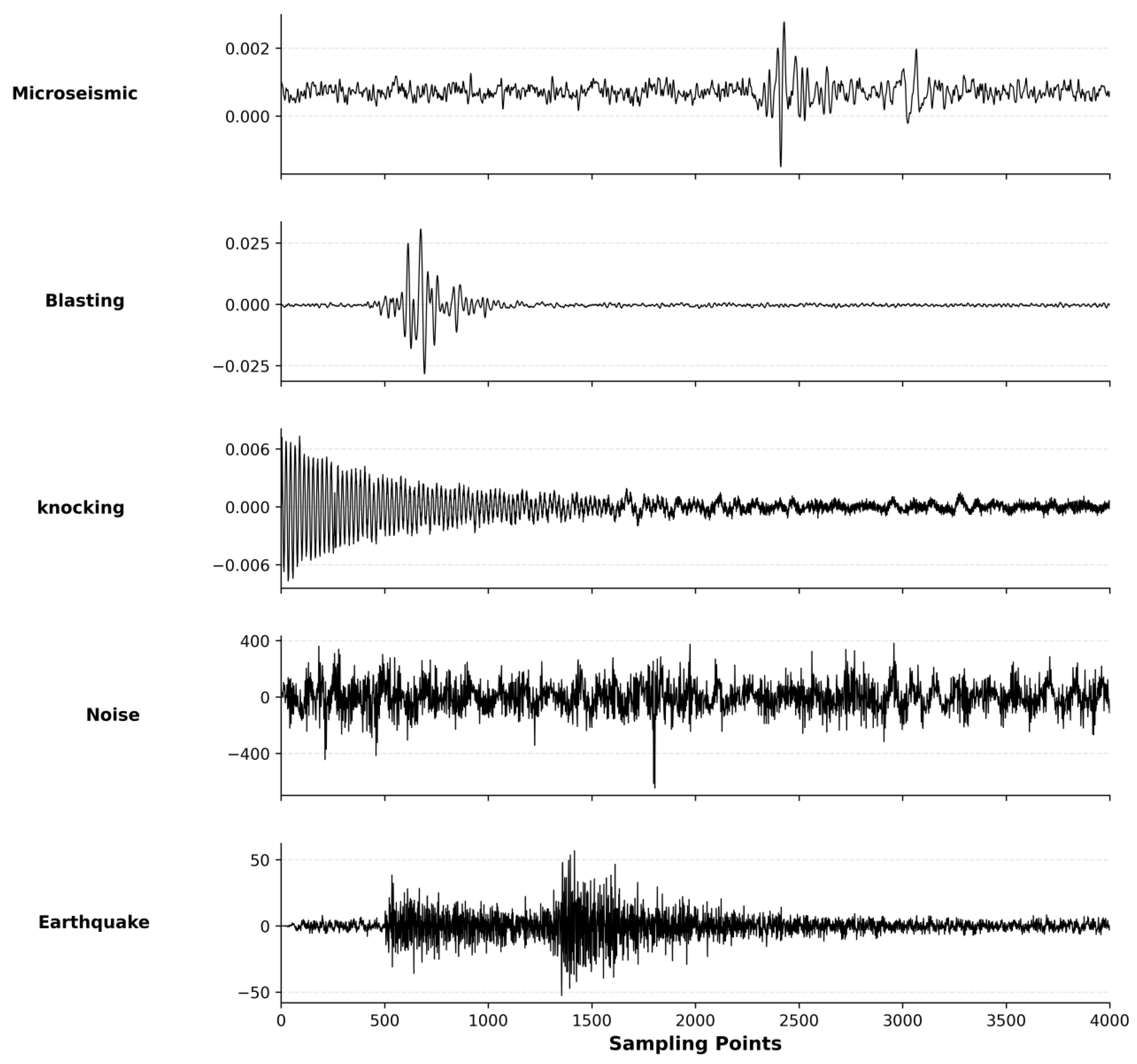
Regarding the dataset specifications, this study covers five typical sample categories: microseismic, knocking, blasting, noise, and earthquake. To ensure class balance during training, 400 representative waveforms were selected for each category, forming a total dataset of 2000 samples. The length of each waveform was uniformly set to 4000 sampling points to maintain consistency in input features. For practical deployment in a working mine, continuous monitoring data can be processed using conventional wave arrival detection algorithms, such as the Short-Time Average/Long-Time Average (STA/LTA) method, to automatically detect potential seismic arrivals. After event triggering, fixed-length waveform segments containing the detected arrival, together with the pre-event noise baseline and post-event coda intervals, are extracted for subsequent analysis. In this study, this 4000-point window length provides sufficient temporal coverage to capture both the pre-event noise floor and the post-event decay characteristics under noisy conditions. Such a windowing strategy allows the generated STFT spectrograms to preserve not only the primary event arrivals but also the surrounding background noise characteristics, thereby providing richer contextual information for classification. Typical time-domain waveforms for each signal type are shown in Figure 1. A comparison reveals significant physical differences among the events regarding amplitude characteristics, frequency distribution, and duration.

Although Figure 1 reveals apparent differences in amplitude, frequency, and duration among the five signal categories, these features exhibit substantial overlaps in practical mine environments with variable SNR, rendering simple threshold-based classification unreliable.

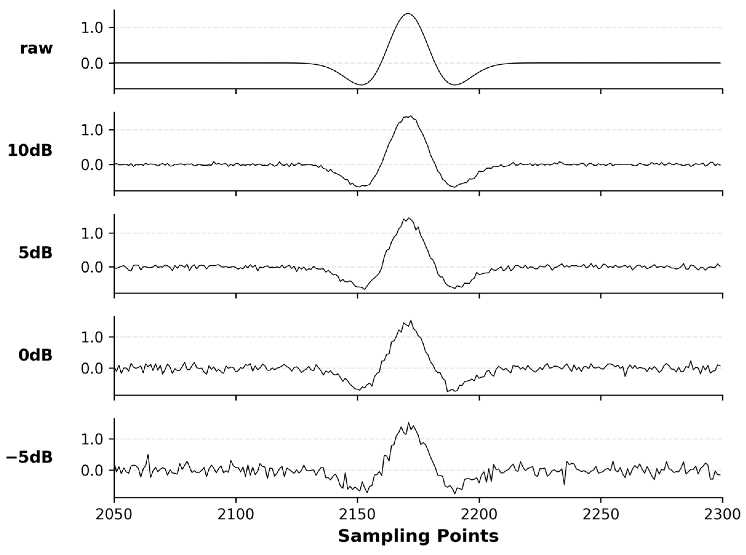
Considering the complexity of mine environments and strong noise interference, this study further enhances recognition robustness through a controlled data augmentation strategy. To verify the model’s performance under extremely low-SNR conditions and eliminate the influence of inherent noise in field data on SNR control precision, Ricker-wavelet-simulated signals were used as clean baseline waveforms [19]. On this basis, multi-gradient training samples with SNRs of 10, 5, 0, and −5 dB were generated by superimposing random Gaussian noise. Figure 2 shows examples of these simulated microseismic signals at different SNR levels. This method enables the model to fully learn the discriminative features of microseismic waveforms against strong noise, thereby ensuring cross-domain generalization in extreme environments and providing a reliable foundation for subsequent weak signal recognition performance evaluation. The generated samples with different SNR levels were combined into a single mixed-noise training set, rather than being segregated into separate fixed-SNR subsets. This strategy ensures that the model encounters varying noise intensities throughout the training process, thereby learning robust feature representations applicable to the fluctuating noise conditions in real mining environments. For quantitative evaluation, dedicated test sets with fixed SNR levels (10 dB, 5 dB, 0 dB, and −5 dB) were employed to assess model performance under controlled noise conditions.

2.2. Signal Preprocessing

A multi-step preprocessing workflow was established to address issues such as inconsistent acquisition equipment, chaotic environmental noise, and obscured time–frequency features. Amplitude normalization was first applied to eliminate systematic differences between devices and facilitate initial model convergence. Band-pass filtering was then used to remove high-frequency noise and isolate the effective frequency range of microseismic signals. Zero-mean unit-variance standardization was implemented to eliminate mean shift and ensure consistent data distribution across samples. Finally, STFT was employed to map one-dimensional time-domain waveforms into two-dimensional spectrograms, enhancing spatial features for robust recognition.

To eliminate equipment discrepancies and accelerate network convergence, max-value normalization was applied to the raw waveforms, scaling the signal to the range of [−1, 1] [20].

However, the necessity of normalization extends beyond equipment discrepancy elimination. In our dataset, the raw amplitude ranges of different signal categories differ by several orders of magnitude: noise signals exhibit peak amplitudes of approximately ±400, whereas microseismic signals are as low as ~0.002. Without amplitude normalization, the STFT spectrograms preserve this extreme dynamic range, which can induce the network to rely on trivial amplitude-based shortcuts rather than learning discriminative time–frequency features. A comparative ablation experiment conducted under identical network configurations confirmed this vulnerability: the model achieved only 35.25% validation accuracy when trained on unnormalized waveforms, whereas incorporating the 1D normalization step improved the accuracy to 99%. This substantial performance gap underscores that normalization is essential not only for training stability but also for guiding the network toward physically meaningful feature representations.

Band-pass filtering served as the second step of preprocessing, with its core function being the selection of the effective frequency range of microseismic signals while filtering out low-frequency interference and high-frequency noise, thereby providing a signal foundation for subsequent feature extraction. In this study, a fifth-order Butterworth band-pass filter with a passband of 1–500 Hz was selected. The lower cutoff frequency of 1 Hz suppresses ultra-low-frequency environmental disturbances. The upper cutoff frequency of 500 Hz ensures that the dominant spectral content of all signal categories involved in this study, including microseismic, blasting, and knocking signals, is retained, while simultaneously suppressing high-frequency noise components outside the useful signal band.

Following filtration, zero-mean unit-variance standardization was required. On the basis of amplitude normalization, this step further eliminated mean offsets and variance discrepancies in the signal. The formula is

$$x^{″}={\displaystyle \frac{x^{\prime }-{\mu }_{x^{\prime }}}{\max ({\sigma }_{x^{\prime }},10^{-8})}}$$

(1)

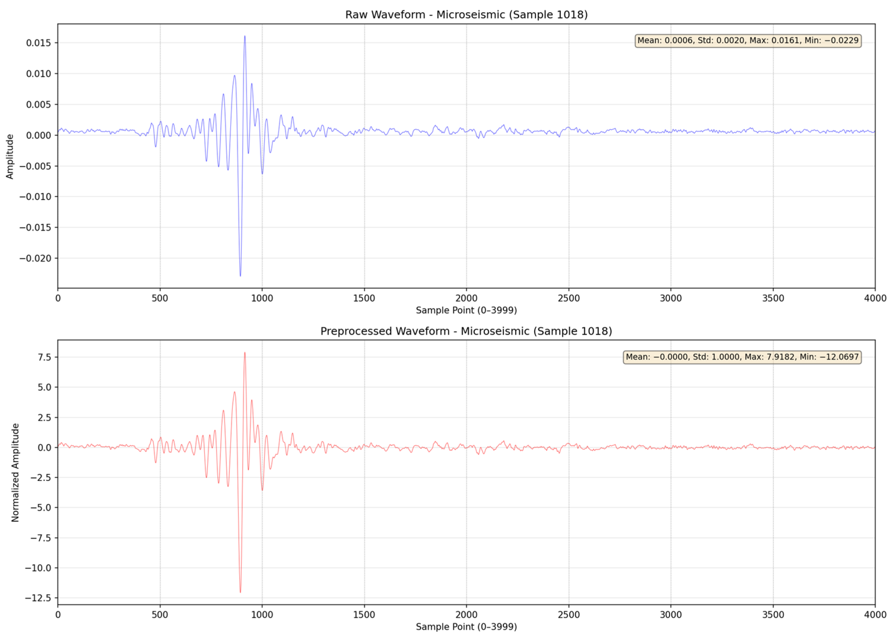
where μ_x′ is the mean of the band-pass filtered signal, σ_x′ is its standard deviation, and the term 10⁻⁸ is introduced to avoid division by zero. After this standardization, the signal’s mean and variance are adjusted to approximately 0 and 1, respectively. This process ensures that the model’s training is not adversely affected by disparate data scales, thereby mitigating risks of slow convergence or overfitting [21], as illustrated in Figure 3.

The distinguishing characteristics of microseismic signals lie in the time–frequency relationship, which is not directly accessible from the raw one-dimensional time-domain waveform. The STFT addresses this by converting a 1D time-domain signal into a 2D time–frequency spectrogram. This transformation visually represents the signal’s frequency distribution across different time points, thereby providing learnable spatial features for the subsequent 2D U-Net model [15].

STFT is a linear time–frequency analysis method [22]. It employs a fixed-length window function to segment a continuous signal into a series of short, overlapping segments in the time domain. This approach sacrifices some dynamic adaptability in time–frequency resolution in exchange for greater computational stability and efficiency. A Fourier transform is then applied to each windowed segment to obtain the local frequency distribution within that specific time window. The results collectively form a two-dimensional time–frequency matrix. The STFT is mathematically defined as follows:

$$X(\tau ,\omega )={\int }_{-\mathrm{\infty }}^{\mathrm{\infty }}x(t)w(t-\tau ){\mathrm{e}}^{-\mathrm{j}\mathsf{\omega }t} \mathrm{d}\mathrm{t}$$

(2)

where x(t) is the one-dimensional signal sequence, τ is the time variable, ω is the analysis frequency, and w(t − τ) is the fixed window function. To suppress spectral leakage caused by time-domain truncation, a Hann window was adopted as the smoothing (tapering) function in this study due to its favorable trade-off between frequency resolution and sidelobe suppression. The window function is defined as

$$\mathrm{w}(\mathrm{t})=\{\begin{array}{c}0.5\left[1-\cos \left({\displaystyle \frac{2\mathsf{\pi }\mathrm{t}}{\mathrm{T}}}\right)\right],0\le \mathrm{t}\le \mathrm{T}\\ 0, \mathrm{otherwise}\end{array}$$

(3)

where T denotes the window duration. In the numerical implementation, the window length was set to 256 sampling points, with an overlap of 128 sampling points. This window function slides along the time axis, thereby extracting the local frequency characteristics of the signal at different time instants.

With a fixed window length and overlap rate set, the STFT was applied to the preprocessed 1D signals to generate their two-dimensional spectrograms. These spectrograms were then uniformly resized to 64 × 64 pixels to ensure consistent input dimensions for the subsequent neural network. Such a time–frequency representation aids in preserving the discriminative features of weak microseismic signals at specific frequency bands and temporal locations, even within a multi-class signal mixture.

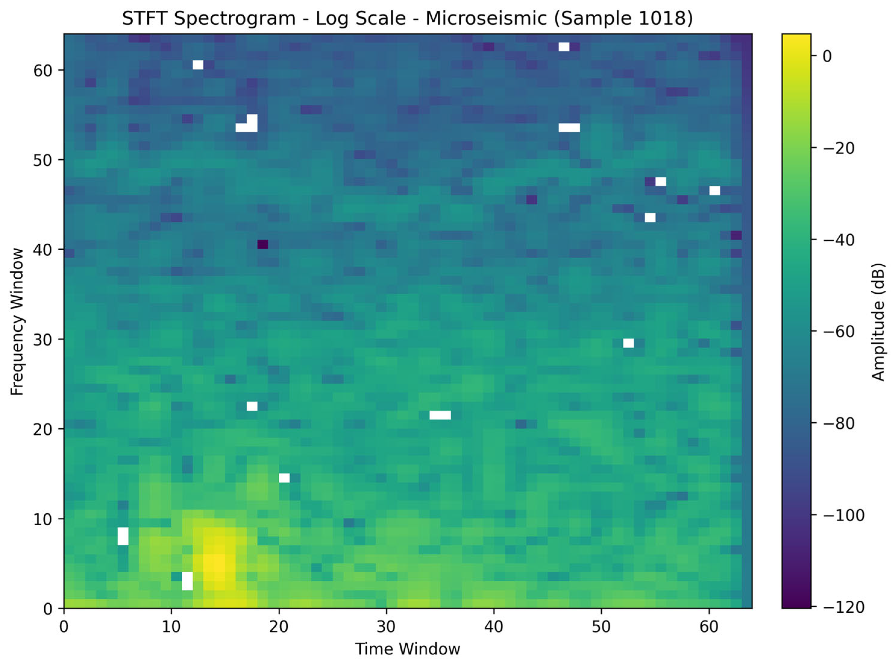
For illustration, the standardized signal from Figure 3 was processed via STFT using a window length of 256 samples and an overlap of 128 samples, followed by interpolation to yield a 64 × 64 time–frequency matrix. Since linear-amplitude representations tend to compress low-energy spectral components into values close to zero, weak signal characteristics are often difficult to observe in linear-scale spectrograms. Therefore, a logarithmic amplitude scale (decibels, dB) was adopted to generate the final spectrogram shown in Figure 4. The logarithmic transformation is defined as

$$X_{\mathrm{d}\mathrm{B}}(\tau ,\omega )=20 {\log }_{10}(\left|X\right(\tau ,\omega \left)\right|+ϵ)$$

(4)

where |$X$(τ, ω)| denotes the linear spectral amplitude obtained from Equation (2), and $ϵ$ = 10⁻⁸ is a small constant introduced to avoid numerical singularity. As shown in Figure 4, the logarithmic representation reveals weak spectral structures that are difficult to observe on a linear scale, including low-amplitude background noise and faint signal coda components. These additional time–frequency details improve the interpretability of microseismic signals and facilitate qualitative analysis of weak signal characteristics. While training the neural network directly with logarithmic-scale spectrograms could potentially enhance the extraction of faint features by balancing the numerical weights of high- and low-energy components, the proposed model retains linear-amplitude spectrograms for training to preserve the original physical energy relationships of the signals, which may be important for subsequent microseismic analysis and engineering applications. Therefore, the logarithmic representation is employed exclusively for visualization in this study, while future work may investigate the potential benefits of logarithmic-scale inputs for model training.

The linear frequency partitioning of the STFT is adopted in this study for three main reasons. First, the FFT-based STFT provides an efficient implementation and is widely used in real-time signal processing applications. Second, although microseismic events are mainly concentrated in the low-frequency range, blasting and knocking signals contain higher-frequency spectral components that are important for classification. Retaining the original linear frequency representation preserves the complete spectral information within the selected frequency band without introducing additional frequency-domain distortions. Third, a linear frequency axis provides a uniform frequency resolution across the entire spectrum, enabling the convolutional layers of the U-Net to learn spectral patterns under a consistent representation.

3. Model Description

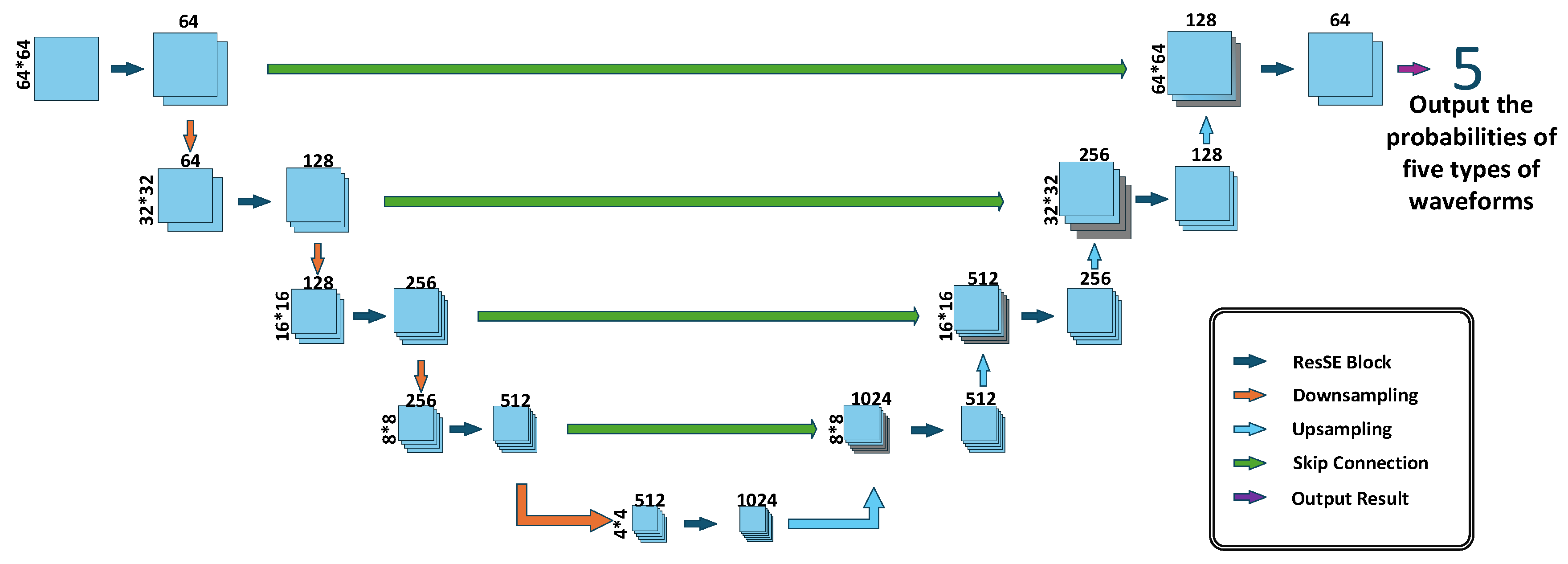
The early warning model proposed in this study for mine dynamic disasters is built upon a U-Net encoder–decoder architecture, enhanced with the Squeeze-and-Excitation (SE) attention mechanism and residual networks. In this architecture, the encoder performs downsampling to extract deep features, while the decoder uses upsampling to restore spatial dimensions. Skip connections are employed to fuse shallow, high-resolution time–frequency details with deep, high-level semantic features. This design provides inherent advantages for feature enhancement and noise suppression when processing weak microseismic signals. The model operates on 64 × 64 single-channel spectrograms derived from microseismic signals via STFT, enabling the joint recognition of five event categories. In the context of mine disaster early warning, accurately identifying microseismic events requires the model not only to capture their intrinsic features but also to robustly distinguish them from other high-energy events. Therefore, a multi-class joint modeling strategy was adopted, which incorporates blasting, knocking, noise, and earthquake signals during training. This approach is designed to improve the overall reliability of microseismic signal recognition.

The model follows an end-to-end learning scheme. It takes the preprocessed time–frequency spectrogram as input and outputs a probability distribution over the five event categories. This design allows the network to autonomously learn discriminative features under complex conditions, thereby establishing a foundation for subsequent performance evaluation in low-SNR scenarios.

3.1. Design of the Residual SE Attention Block (Res-SE)

To balance deep feature extraction capability with training stability, a Res-SE unit was designed. This unit integrates the SE attention module into a residual learning framework, creating a cohesive structure that sequentially performs feature extraction, channel calibration, and residual reconstruction. Utilizing a parallel branch design, it achieves nonlinear mapping of high-dimensional features while leveraging the attention mechanism to adaptively highlight key seismic signatures and suppress background noise [23,24].

The main branch consisted of two consecutive 3 × 3 convolutional layers for feature extraction, each followed by Batch Normalization to accelerate convergence. The LeakyReLU activation function was employed to mitigate the “dying ReLU” problem and maintain continuous gradient flow. Although the input STFT magnitude spectrogram consists of strictly non-negative values, the intermediate feature maps generated by subsequent convolutional and batch normalization layers inevitably contain both positive and negative values due to negative filter weights and data centering. Its mathematical expression is as follows:

$$\mathrm{L}\mathrm{e}\mathrm{a}\mathrm{k}\mathrm{y}\mathrm{R}\mathrm{e}\mathrm{L}\mathrm{U}(x)=\{\begin{array}{ll}x,& x\ge 0\\ \mathsf{\alpha }\cdot x,& x<0\end{array}$$

(5)

where α is the negative slope. This property ensures that a small gradient is propagated even for negative inputs, preventing neurons from becoming permanently inactive. This mechanism helps preserve and propagate faint feature representations of weak microseismic signals within deep network architectures. The selection of LeakyReLU is primarily motivated by its ability to maintain gradient propagation in deep networks, which is particularly beneficial for preserving weak feature representations. In the present study, the proposed model achieved satisfactory performance under low-SNR conditions, indicating that the selected activation function is suitable for the target task.

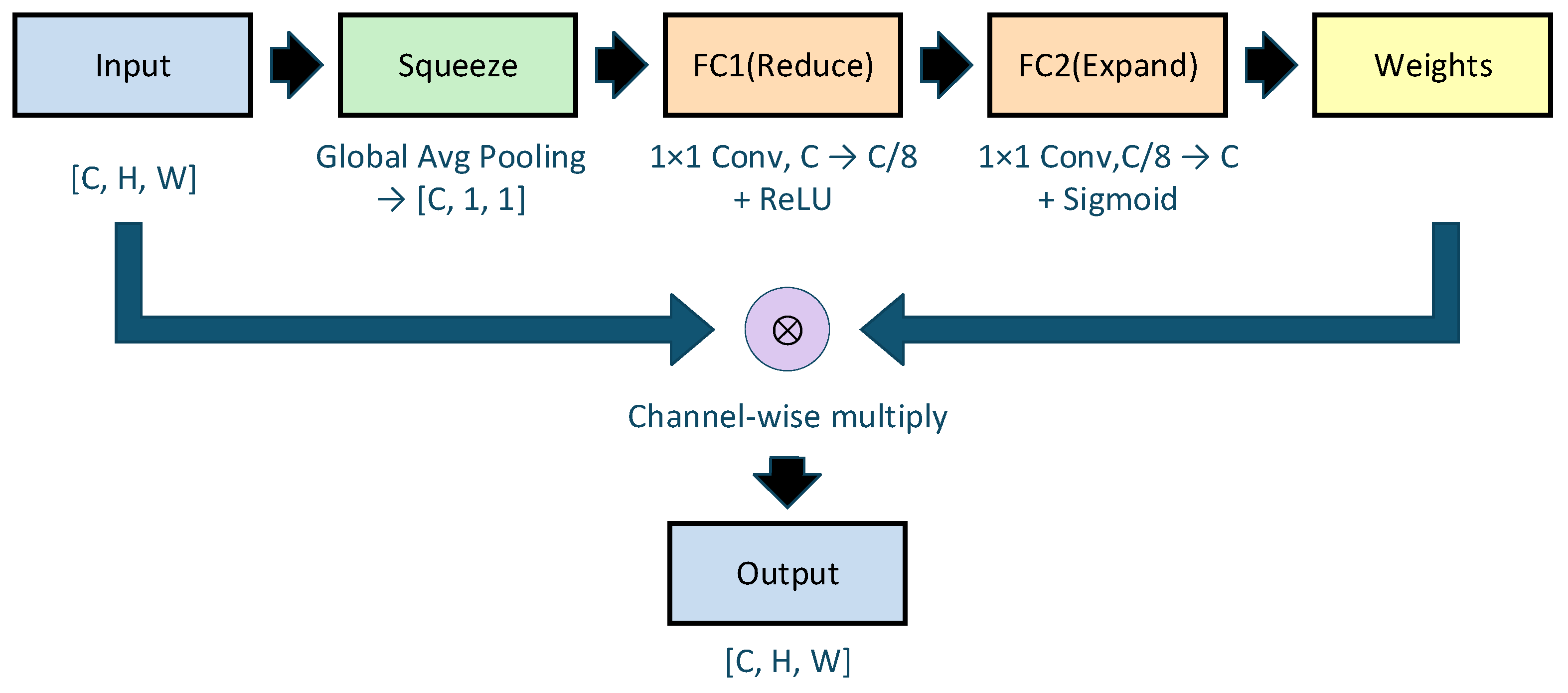
Subsequently, an SE module was utilized to recalibrate the feature maps produced by the main branch. It first captures the global context via global average pooling and then adaptively generates channel-wise weights through convolutional layers, achieving refined feature representation and channel-level optimization.

The shortcut branch was used to construct the residual connection, addressing common deep network issues such as performance degradation and gradient vanishing. When the input and output channel counts of the main branch were equal, an identity mapping directly passed the original features. Otherwise, a 1 × 1 convolution was employed to adjust the feature dimensions. This ensures that the recalibrated output from the main branch can be element-wise added to the features from the shortcut branch. This mechanism preserves feature propagation continuity and effectively enhances the model’s robustness for weak signal recognition.

The SE module was embedded within this residual path. It operates by first aggregating spatial information through global average pooling, followed by two fully connected layers that adaptively learn channel weights. Its operation is formulated as

$$z_{\mathrm{c}}={\displaystyle \frac{1}{\mathrm{H}\times \mathrm{W}}}{\displaystyle \sum _{i=1}^{\mathrm{H}}}{\displaystyle \sum _{j=1}^{\mathrm{W}}}{x}_{i,j,c}$$

(6)

where x_i,j,c represents the feature value at position (i, j) in the c-th, and z_c is the output of the global average pooling over the spatial dimensions for that channel. This operation effectively captures the global energy distribution across specific frequency channels, reducing the interference of local noise on feature discrimination. The detailed structure of the SE module is illustrated in Figure 5.

The first fully connected layer adaptively learns channel weights through a compression and recalibration mechanism. A weight vector was then generated via a Sigmoid activation function to recalibrate the feature maps, thereby enhancing the response to key microseismic frequencies.

3.2. Encoder–Decoder Network Architecture

The encoder comprised four downsampling stages. At each stage, features were first extracted by a Res-SE block and then downsampled by a 2 × 2 max-pooling layer. As the network deepened, the spatial size of the feature maps was halved stage by stage, while the number of channels was doubled. A dropout layer was added after the fourth downsampling stage to mitigate overfitting.

The decoder similarly consisted of four stages. It used transposed convolution (deconvolution) to progressively upsample the feature maps. At each decoder stage, a skip connection concatenated the corresponding shallow high-resolution features from the encoder with the upsampled deep semantic features. The fused features were then processed by a Res-SE block for further refinement and channel reduction. This design effectively compensates for the loss of fine time–frequency textures, which is critical for identifying weak microseismic signals.

The classification head compresses the feature map output by the decoder into a feature vector via global average pooling. Subsequently, a two-layer fully connected network outputs the category scores corresponding to the five event types, which are used for subsequent multi-class discrimination.

The overall architecture is depicted in Figure 6. This design enables the model to suppress the dominant influence of high-energy interference events while simultaneously preserving the subtle time–frequency characteristics of weak microseismic signals under low-SNR conditions.

3.3. Training Parameters and Strategy

The inputs for model training consist of preprocessed time–frequency spectrograms and their corresponding labels, both of which were segmented into 64 × 64 patches. The optimization algorithm employs AdamW with the integration of weight decay. This configuration effectively addresses the issues of gradient sparsity and noise in the model, provides a robust adaptive learning rate, accelerates convergence, and enhances overall training performance. The initial learning rate was set to 1 × 10⁻³, with a weight decay coefficient of 5 × 10⁻⁴ to implement adaptive optimization for stochastic gradient descent.

To prevent overfitting during the training process, a dropout rate was applied between the fully connected layers of the classification head, further reducing inter-neuron dependency. Learning rate scheduling follows the ReduceLROnPlateau strategy, utilizing validation accuracy as the monitoring metric. If the validation accuracy fails to improve for a specified number of consecutive epochs, the learning rate was multiplied by a factor of 0.5, assisting the model in escaping local optima during convergence stagnation.

The cross-entropy loss function was selected to accommodate the multi-class classification task involving five types of signals. Cross-entropy effectively measures the divergence between the predictive distribution and the ground truth distribution, guiding the network to optimize its parameters and minimize classification error.

To balance computational efficiency with the stability of training results, the total number of epochs was set to 80, and the batch size was fixed at 32. This setup maintains an optimal equilibrium between computing speed and memory footprint, avoiding excessively long training durations caused by overly small batch sizes or the degradation of generalization performance resulting from excessively large ones. All experiments were implemented using the PyTorch framework (version 2.7.1) and executed on NVIDIA GPU to ensure the stability and high efficiency of both model training and inference.

4. Results and Discussion

This chapter systematically validates the capability of the proposed method to concurrently mitigate misidentification and missed detection in mine dynamic disaster early warning scenarios through multi-class recognition and weak-signal comparative experiments.

4.1. Experimental Setup

All samples underwent standardized preprocessing and were subsequently divided into training and validation sets using an 8:2 stratified ratio. The AdamW optimizer was employed during the training process, with an initial learning rate of $1\times {10}^{-3}$ and a weight decay coefficient of $5\times {10}^{-4}$. Furthermore, the ReduceLROnPlateau strategy was introduced for dynamic learning rate adjustment, and the training was conducted for a total of 80 epochs.

4.2. Overall Recognition Performance and Core Microseismic Metrics

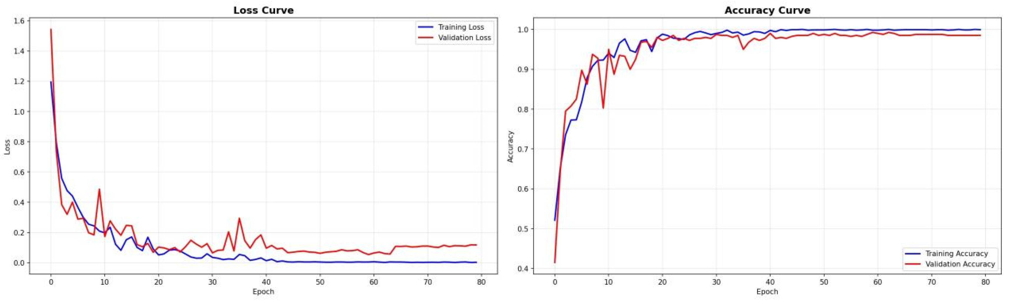
The training results are illustrated in Figure 7. The model demonstrates rapid and stable convergence without significant overfitting. Stability was achieved around the 40th epoch, ultimately yielding an overall recognition accuracy of 99.25% on the validation set.

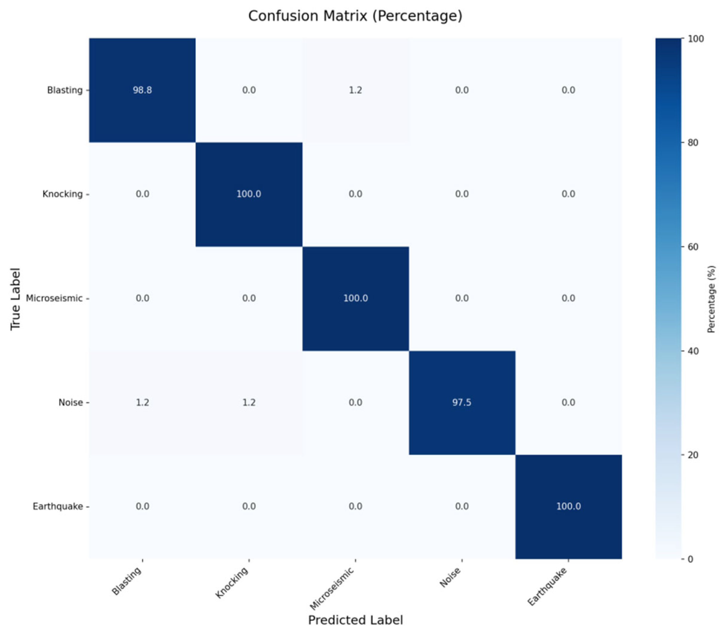
To further assess the model’s recognition capability for individual signal categories, Figure 8 presents the confusion matrix for the five signal types on the validation set. The model demonstrated exceptional performance across all categories. Notably, it attained a perfect 100% classification accuracy for microseismic, knocking, and earthquake signals. For microseismic signals—the most critical indicator for mine safety—the model achieved a recall of 100%. The matrix confirms that all true microseismic samples were correctly identified, with zero instances misclassified as noise or interference, thereby substantially reducing the risk of undetected disasters.

Regarding precision, the microseismic category reached 98.77%. Inspecting the misclassifications reveals that only a very small number of blasting samples were mistaken for microseismic ones. This margin of error is considered acceptable in engineering practice; since the primary objective of an early-warning system is to prevent catastrophic events, maintaining high sensitivity for microseismic detection takes precedence over the minor risk of false alarms.

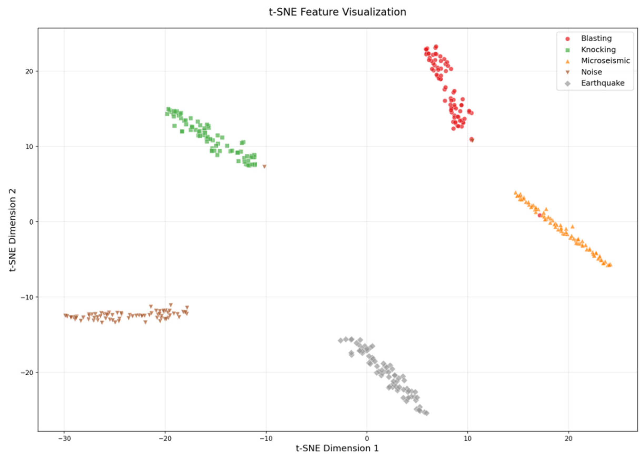
The effectiveness of the learned features was further validated by visualizing the high-dimensional feature space using t-SNE, as shown in Figure 9. The five signal categories formed well-separated, distinct clusters with minimal overlap. This high separability indicates that the model successfully learned the intrinsic time–frequency characteristics distinguishing each signal type. Moreover, interference signals such as blasting and knocking were positioned far from the microseismic cluster. This effective disentanglement explains the low misclassification rate observed in the confusion matrix. Additionally, the tight clustering and high intra-class cohesion underscore the consistency and robustness of the feature extraction process.

To quantitatively evaluate the model’s prediction confidence and the distinctiveness between the target class and its closest competitor, the classification margin (M) was calculated for each sample on the validation set. The margin is defined as

$$M=P_{first}-P_{second}$$

(7)

where $P_{first}$ and $P_{second}$ represent the highest and second-highest predicted probabilities from the softmax layer, respectively. A margin close to 1.0 indicates that the network categorizes the signal with high confidence and minimal ambiguity with respect to competing classes.

Table 1. Statistical metrics of classification margins for the five signal categories.

Class	Samples	Mean	Median	Max	Min
Blasting	80	0.98069	0.99995	1.00000	0.27181
Knocking	80	0.99998	0.99999	1.00000	0.99978
Microseismic	80	0.98552	0.99966	1.00000	0.69509
Noise	80	0.98953	0.99999	1.00000	0.23061
Earthquake	80	0.99095	1.00000	1.00000	0.43373

lists the statistical metrics of the classification margins for the five signal categories.

As demonstrated in Table 1, the median classification margins for all five categories are exceptionally close to 1.00000, while the mean margins consistently exceed 0.98, indicating that the proposed model distinguishes the target category with high confidence for the vast majority of samples. Notably, the noise category exhibits a relatively low minimum margin of 0.23061. This observation suggests that certain noise samples share partial time–frequency characteristics with microseismic or blasting events, leading to increased classification ambiguity. Nevertheless, the median margin for noise remains as high as 0.99999, indicating that such ambiguous cases are rare and do not affect the overall reliability of the classifier.

4.3. Comparative Experimental Analysis of Weak Microseismic Signal Recognition

In practical mine monitoring environments, microseismic signals are frequently subject to complex conditions where multi-source interference and background noise coexist. Since the SNR fluctuates significantly with varying working conditions, model robustness across different SNR levels is a critical determinant of early warning system practicality. To verify the applicability of the model in complex environments and clarify the superiority of the proposed STFT and Residual SE-attention U-Net (STFT-ResU-Net) in processing weak signals, this study designed four SNR levels of 10 dB, 5 dB, 0 dB, and −5 dB, using Ricker wavelet-synthesized signals to simulate monitoring environments ranging from low to intense noise. Furthermore, three groups of comparative models were constructed for ablation experiments to evaluate performance variations as the SNR decreased from 10 dB to −5 dB.

Regarding the comparative model configurations, four architectures with distinct structures were established for comprehensive evaluation, as summarized in

Table 2. Configuration of comparative models.

Model Name	Input Features	Network Architecture	Core Component/Difference	Validation Purpose
Model A	1D Time-Domain Waveform	U-Net (1D)	Res-SE Module	Verify the necessity of STFT
Model B	2D STFT	ResNet-18	Pure Encoder (No Decoder)	Verify the advantages of U-Net architecture
Model C	2D STFT	U-Net (2D)	No Res-SE Module	Verify the effect of Res-SE Module
Model D	2D STFT	U-Net (2D)	Res-SE Module	Verification of the complete solution

. Model A is the 1D Res-SE U-Net, which directly takes one-dimensional time-domain waveforms as input and incorporates Res-SE modules to verify the necessity of STFT-based time–frequency features. Model B is ResNet-18, which uses 2D STFT spectrograms as input and adopts a classic deep convolutional architecture to evaluate the U-Net architecture’s capability in preserving weak features. Model C is the standard 2D U-Net, which also uses 2D STFT spectrograms but excludes Res-SE modules to verify the noise suppression effect of the attention mechanism. Model D is STFT-ResU-Net, representing the complete proposed scheme that integrates STFT, the U-Net architecture, and Res-SE modules.

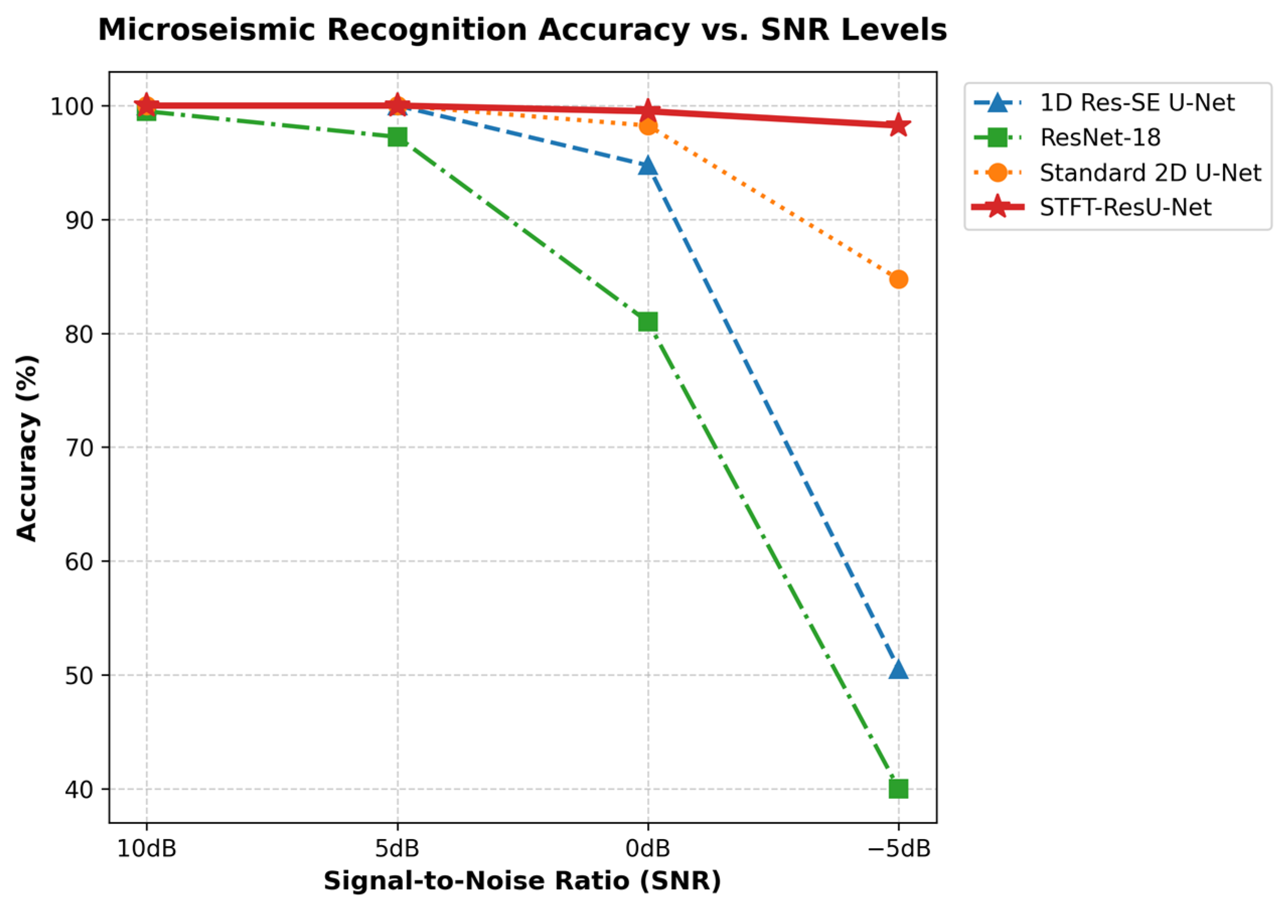
As shown in Figure 10, the proposed STFT-ResU-Net model exhibits remarkable robustness. It achieved perfect 100% accuracy at high SNRs of 5 dB and 10 dB. When the SNR dropped to 0 dB, the accuracy experienced only a marginal decline to 99.50%. Crucially, even under the extreme noise condition of −5 dB, the model maintained a high accuracy of 98.25%.

A comparative analysis underscores this superiority. At −5 dB, the accuracy of the 1D U-Net plummeted to 50.50%, trailing the proposed model by 47.75 percentage points. This sharp contrast indicates that 1D time-domain features become severely aliased and indistinguishable under strong noise. Conversely, STFT preprocessing, by mapping signals into the time–frequency domain, preserves the discriminative energy distribution of microseismic events in specific frequency bands, establishing it as a fundamental prerequisite for accurate weak-signal recognition. The skip connections in the U-Net architecture proved vital for retaining weak features. At −5 dB, ResNet-18 attained a mere 40.00% accuracy, which was even lower than the 1D U-Net, highlighting how deep downsampling causes severe loss of subtle time–frequency textures. In comparison, the standard 2D U-Net achieved 84.75% accuracy, confirming that skip connections effectively transmit high-resolution shallow details to deeper layers, thereby preventing the loss of faint features.

Furthermore, the Res-SE module substantially enhanced robustness. Integrating this module into the standard 2D U-Net boosted the −5 dB accuracy dramatically from 84.75% to 98.25%. This significant improvement demonstrates the efficacy of the SE attention mechanism, which suppresses interference from background noise channels by adaptively recalibrating channel weights, enabling the model to focus precisely on the salient energy regions of microseismic signals.

Regarding computational efficiency, as detailed in

Table 3. Performance comparison of different models for microseismic signal recognition under varying SNR levels.

Model	Accuracy (10 dB)	Accuracy (5 dB)	Accuracy (0 dB)	Accuracy (−5 dB)	Inference Time (ms)
1D Res-SE U-Net	100%	100%	94.75%	50.50%	4.06
ResNet-18	99.50%	97.25%	81.00%	40.00%	2.48
Standard 2D U-Net	100%	100%	98.25%	84.75%	2.14
STFT-ResU-Net	100%	100%	99.50%	98.25%	6.59

, the average inference time was 6.59 ms per sample. Although this is higher than that of ResNet-18, the modest computational overhead is overwhelmingly justified by the model’s transformative performance gains.

Furthermore, to explore how noise intensity affects prediction certainty, the classification margins of the complete STFT-ResU-Net model were analyzed across different SNR levels.

Table 4. Classification margins of the proposed model under different SNR levels.

SNR (dB)	Samples	Mean	Median	Max	Min
10	400	1.00000	1.00000	1.00000	0.99999
5	400	0.99999	1.00000	1.00000	0.99737
0	400	0.99516	1.00000	1.00000	0.11946
−5	400	0.99181	1.00000	1.00000	0.08555

presents the sample size, mean, median, maximum, and minimum classification margins under varying noise conditions.

The results in Table 4 demonstrate that the predictions remain highly distinguishable under different noise levels. At SNRs of 5 dB and 10 dB, both the mean and median margins are nearly 1.00000, indicating highly confident predictions. As the SNR decreases to 0 dB and −5 dB (corresponding to increased noise intensity), the minimum margins decrease to 0.11946 and 0.08555, respectively, reflecting the increasing difficulty of distinguishing signals that are strongly masked by noise. Importantly, the vast majority of samples still maintain high confidence, as evidenced by mean margins of 0.99516 and 0.99181, with medians remaining at 1.00000. These results indicate that the proposed STFT-ResU-Net framework maintains stable classification performance and strong class separability even under extremely low-signal-to-noise-ratio conditions.

5. Conclusions

By deeply integrating the STFT with a Residual SE-attention U-Net architecture, this study has developed a microseismic signal recognition model tailored for mine dynamic disaster early warning, achieving the synergistic expression of time–frequency detailed features and high-level semantic information. The SE attention mechanism adaptively highlights the key discriminative features of microseismic signals while effectively suppressing noise redundancy, ensuring both recognition precision and the computational efficiency essential for real-time monitoring.

Comprehensive experimental results demonstrate that, under small-sample conditions, where five signal categories (microseismic, knocking, blasting, noise, and earthquake) are involved in training with only 400 samples per category, the proposed method maintains stable and high-precision multi-class recognition performance, yielding an overall accuracy of 99.25% on the validation set. Further analysis reveals that by incorporating multiple types of typical interference signals for joint modeling, the model exhibits exceptional discriminative capabilities in complex monitoring environments. The cross-misidentification rate between various interference events and microseismic signals is significantly reduced, thereby enhancing the reliability of mine dynamic disaster early warning results.

Weak signal experiments conducted on this basis further validate the model’s robustness. Even under an extreme SNR of −5 dB, the model maintains a 98.25% recognition accuracy for microseismic signals. This indicates that the proposed method possesses stable and reliable detection capabilities for weak microseismic signals, even when they are obscured by intense noise.

In conclusion, the method proposed in this study demonstrates high recognition accuracy, superior noise robustness, and excellent engineering applicability under small-sample constraints. It provides a feasible technical path for the engineering implementation of microseismic recognition modules in mine dynamic disaster early warning systems.

References

1. Li, Z.; Qiao, D.; Yang, T.; Wang, J.; Chen, H. Event recognition technology and short-term rockburst early warning model based on microseismic monitoring and ensemble learning. Sci. Rep. 2025, 15, 18674. [Google Scholar] [CrossRef]
2. Ma, T.; Tang, C.; Liu, F.; Zhang, S.; Feng, Z. Microseismic monitoring, analysis and early warning of rockburst. Geomat. Nat. Hazards Risk 2021, 12, 2956–2983. [Google Scholar] [CrossRef]
3. Huang, W.; Wang, R.; Li, H.; Chen, Y. Unveiling the signals from extremely noisy microseismic data for high-resolution hydraulic fracturing monitoring. Sci. Rep. 2017, 7, 11996. [Google Scholar] [CrossRef] [PubMed]
4. Peng, P.; He, Z.; Wang, L.; Jiang, Y. Microseismic records classification using capsule network with limited training samples in underground mining. Sci. Rep. 2020, 10, 13925. [Google Scholar] [CrossRef] [PubMed]
5. Dong, L.; Tang, Z.; Li, X.; Chen, Y.; Xue, J. Discrimination of mining microseismic events and blasts using convolutional neural networks and original waveform. J. Cent. South Univ. 2020, 27, 3078–3089. [Google Scholar] [CrossRef]
6. Duan, Y.; Shen, Y.; Canbulat, I.; Luo, X.; Si, G. Classification of clustered microseismic events in a coal mine using machine learning. J. Rock Mech. Geotech. Eng. 2021, 13, 1256–1273. [Google Scholar] [CrossRef]
7. Pu, Y.; Apel, D.B.; Hall, R. Using machine learning approach for microseismic events recognition in underground excavations: Comparison of ten frequently-used models. Eng. Geol. 2020, 268, 105519. [Google Scholar] [CrossRef]
8. Wang, J.; Teng, T. Artificial neural network-based seismic detector. Bull. Seismol. Soc. Am. 1995, 85, 308–319. [Google Scholar] [CrossRef]
9. Maity, D.; Aminzadeh, F.; Karrenbach, M. Novel hybrid artificial neural network based autopicking workflow for passive seismic data. Geophys. Prospect. 2014, 62, 834–847. [Google Scholar] [CrossRef]
10. Mousavi, S.M.; Horton, S.P.; Langston, C.A.; Samei, B. Seismic features and automatic discrimination of deep and shallow induced-microearthquakes using neural network and logistic regression. Geophys. J. Int. 2016, 207, 29–46. [Google Scholar] [CrossRef]
11. Perol, T.; Gharbi, M.; Denolle, M. Convolutional neural network for earthquake detection and location. Sci. Adv. 2018, 4, e1700578. [Google Scholar] [CrossRef] [PubMed]
12. Seydoux, L.; Balestriero, R.; Poli, P.; de Hoop, M.; Campillo, M.; Baraniuk, R. Clustering earthquake signals and background noise in continuous seismic data with unsupervised deep learning. Nat. Commun. 2020, 11, 3972. [Google Scholar] [CrossRef] [PubMed]
13. Anikiev, D.; Birnie, C.; Waheed, U.; Alkhalifah, T.; Gu, C.; Verschuur, D.J.; Eisner, L. Machine learning in microseismic monitoring. Earth-Sci. Rev. 2023, 239, 104371. [Google Scholar] [CrossRef]
14. Ma, C.; Ran, X.; Xu, W.; Yan, W.; Li, T.; Dai, K.; Wan, J.; Lin, Y.; Tong, K. Fine Classification Method for Massive Microseismic Signals Based on Short-Time Fourier Transform and Deep Learning. Remote Sens. 2023, 15, 502. [Google Scholar] [CrossRef]
15. Jiang, J.; Stankovic, V.; Stankovic, L.; Parastatidis, E.; Pytharouli, S. Microseismic Event Classification With Time-, Frequency-, and Wavelet-Domain Convolutional Neural Networks. IEEE Trans. Geosci. Remote Sens. 2023, 61, 1–14. [Google Scholar] [CrossRef]
16. Liu, D.m.; Zhang, J.; Zhao, B.; Gao, L.; Zhou, H.; Cheng, Z.; Chen, L.; Li, M. Research on computational propagation and identification of mine microseismic signals based on deep learning. PLoS ONE 2025, 20, 0334641. [Google Scholar] [CrossRef] [PubMed]
17. Wei, M.; Sun, X.; Zong, J. Time–Frequency Domain Seismic Signal Denoising Based on Generative Adversarial Networks. Appl. Sci. 2024, 14, 4496. [Google Scholar] [CrossRef]
18. Mousavi, S.M.; Sheng, Y.; Zhu, W.; Beroza, G.C. STanford EArthquake Dataset (STEAD): A Global Data Set of Seismic Signals for AI. IEEE Access 2019, 7, 179464–179476. [Google Scholar] [CrossRef]
19. Wang, T.; Trugman, D.; Lin, Y. SeismoGen: Seismic waveform synthesis using GAN with application to seismic data augmentation. J. Geophys. Res. Solid Earth 2021, 126, e2020JB020077. [Google Scholar] [CrossRef]
20. Chernykh, V.; Stepnov, A.A.; Lukyanova, O. Data preprocessing for machine learning in seismology. In Proceedings of the VI International Conference Information Technologies and High-Performance Computing (ITHPC-2021), Khabarovsk, Russia, 14–16 September 2021; pp. 119–123. [Google Scholar]
21. Zhang, B.; Wu, H.; Yao, J.; Wang, Y. A strategy for preparing training data for machine learning for seismic noise reduction. Geoenergy Sci. Eng. 2025, 250, 213817. [Google Scholar] [CrossRef]
22. Leiber, M.; Barrau, A.; Marnissi, Y.; Abboud, D. A differentiable short-time Fourier transform with respect to the window length. In Proceedings of the 2022 30th European Signal Processing Conference (EUSIPCO), Belgrade, Serbia, 29 August–2 September 2022; pp. 1392–1396. [Google Scholar]
23. Hu, J.; Shen, L.; Sun, G. Squeeze-and-Excitation Networks. In Proceedings of the 2018 IEEE/CVF Conference on Computer Vision and Pattern Recognition, Salt Lake City, UT, USA, 18–22 June 2018; pp. 7132–7141. [Google Scholar]
24. He, K.; Zhang, X.; Ren, S.; Sun, J. Deep Residual Learning for Image Recognition. In Proceedings of the 2016 IEEE Conference on Computer Vision and Pattern Recognition (CVPR), Las Vegas, NV, USA, 27–30 June 2016; pp. 770–778. [Google Scholar]
Figure 1. Five representative signal samples.
Applsci 16 06417 g001
Figure 2. Simulated microseismic signals at different SNRs.
Applsci 16 06417 g002
Figure 3. Raw microseismic waveform and the standardized waveform after preprocessing.
Applsci 16 06417 g003
Figure 4. Logarithmic-scale STFT spectrogram of the preprocessed microseismic signal.
Applsci 16 06417 g004
Figure 5. Structure of the SE attention module.
Applsci 16 06417 g005
Figure 6. Overall network architecture.
Applsci 16 06417 g006
Figure 7. Training curves of accuracy and loss.
Applsci 16 06417 g007
Figure 8. Confusion matrix for the recognition of five signal categories.
Applsci 16 06417 g008
Figure 9. 2D t-SNE visualization of feature distribution.
Applsci 16 06417 g009
Figure 10. Microseismic recognition accuracy of different models under varying SNRs.
Applsci 16 06417 g010