


Abstract
PM2.5 is a major air pollutant that threatens urban air quality and public health. Its concentration is influenced by both meteorological conditions and air pollutants, exhibiting complex nonlinear and temporal characteristics. Traditional statistical methods are limited in their ability to model complex relationships among environmental variables, while machine learning models still require improvements in hyperparameter optimization and interpretability. Therefore, developing an accurate and interpretable PM2.5 estimation model remains an important research objective. This study used daily air-quality and meteorological data collected in Wuhan from 2016 to 2025 to develop six machine learning models: Decision Tree (DT), Random Forest (RF), XGBoost, LightGBM, Support Vector Machine (SVM), and Multilayer Perceptron (MLP). The Particle Swarm Optimization (PSO) algorithm was employed to optimize the hyperparameters of these models. By comparing the root mean square error (RMSE), coefficient of determination (R2), and mean absolute error (MAE) of each model on both the training and test sets, the PSO-MLP model was identified as the best-performing model. Furthermore, the Shapley Additive Explanations (SHAP) method was applied to perform both global and local interpretation analyses of the best-performing model. The results indicate that the PSO-MLP model achieved the highest estimation performance among all evaluated models, with an R2 value of 0.746 on the test set. SHAP analysis revealed that CO, Temperature (Temp), and NO2 were the most influential predictors, while all variables exhibited distinct nonlinear relationships with PM2.5 concentration. These findings may contribute to PM2.5 concentration estimation, air-quality management, and environmental decision-making.
1. Introduction
The sharp increase in air pollution, particularly fine particulate matter (PM2.5), has become a major environmental challenge threatening global public health and hindering sustainable social development [1,2]. Due to its small aerodynamic diameter (less than 2.5 micrometers) and large specific surface area, PM2.5 can adsorb toxic substances and penetrate the lung barrier into the bloodstream, thereby increasing the incidence of cardiovascular and respiratory diseases [3,4] and the risk of premature death [5]. Therefore, constructing a high-precision and highly reliable PM2.5 concentration estimation model to accurately capture its temporal variation patterns is of critical practical significance for governments to formulate effective air pollution prevention and control strategies and for public health early warning [6,7].
In the study of PM2.5 concentration estimation, traditional methods primarily fall into two categories: numerical models based on physicochemical mechanisms (e.g., WRF-Chem [8], CMAQ [9]) and traditional statistical models (e.g., multiple linear regression (MLR) [10,11], autoregressive integrated moving average (ARIMA) [12,13]). Physical models can simulate atmospheric diffusion and chemical transport processes, but they are structurally complex, require high-precision meteorological and surface emission inventory data, and are extremely computationally expensive [7,14,15]. On the other hand, traditional statistical models are mostly based on linear assumptions. Since PM2.5 concentration is influenced by both natural factors and human activities and exhibits highly nonlinear and non-stationary characteristics, traditional statistical models often suffer from limited estimation accuracy when dealing with complex relationships [16,17].
In recent years, with the rapid development of artificial intelligence technology, data-driven machine learning models have been widely applied in the field of air quality prediction [18,19]. Machine learning methods can automatically learn feature patterns from large amounts of data, overcoming the limitations of traditional linear approaches. For example, models such as Decision Tree (DT) [20], Random Forest (RF) [21], Support Vector Machine (SVM) [22,23], and Multilayer Perceptron (MLP) [24], as well as XGBoost [25] and LightGBM [26] based on gradient boosting mechanisms, have demonstrated significant advantages in PM2.5 estimation due to their excellent performance in handling high-dimensional data and capturing complex nonlinear relationships [1]. However, the performance of machine learning models heavily depends on the proper configuration of hyperparameters. Manual tuning is not only time-consuming and labor-intensive but also makes it difficult to identify optimal hyperparameter combinations [27]. To address this issue, heuristic swarm intelligence optimization algorithms, particularly Particle Swarm Optimization (PSO) [28], have been widely introduced for automated hyperparameter optimization. By simulating the foraging behavior of biological populations and iteratively updating particle positions based on individual and global best solutions, the PSO algorithm can help avoid local optima and improve the accuracy and generalization ability of estimation models [19,29,30].
Although machine learning and deep learning models have achieved significant breakthroughs in estimation accuracy, many of them still operate as “black-box” models, lacking sufficient transparency and interpretability. This makes it difficult for the environmental research community to directly validate and understand the physicochemical driving mechanisms behind changes in PM2.5 concentration [29]. In practical applications, clarifying the direction and relative importance of meteorological conditions and related air pollution indicators affecting PM2.5 concentration is important for understanding regional pollution patterns and implementing effective pollution control measures. In recent years, the SHAP method [31] has provided a unified theoretical foundation for overcoming this “black-box” limitation. Based on game theory, SHAP assigns consistent and locally accurate contribution values to each input feature. It not only provides the global importance ranking of meteorological and pollution factors but also reveals their positive or negative effects on PM2.5 concentration [32]. It is worth noting that, in recent years, time-series deep learning models such as LSTM and Transformer have been widely used in estimation research. However, these methods typically rely on time-lag features. Existing studies have shown that the introduction of time-lag features may increase the complexity of model interpretation [33,34].
As a major city in central China, Wuhan is one of the core cities in the middle reaches of the Yangtze River urban agglomeration. PM2.5 concentration changes are influenced not only by local emissions from industrial production, transportation, and residential activities, but also by the regional transport of pollutants from surrounding areas, exhibiting complex nonlinear and seasonal characteristics [35]. Meanwhile, Wuhan is located in a subtropical monsoon climate zone, where significant seasonal differences exist in atmospheric diffusion conditions, boundary layer structure, and pollutant transport processes. This makes Wuhan a representative study area for investigating PM2.5 concentration patterns and their driving mechanisms. Currently, few studies have conducted long-term and systematic comparisons of multiple machine learning models combined with in-depth attribution analysis for this region [7,36].
Based on the above background, this study took Wuhan as the study area and used daily air quality and meteorological observation data from 2016 to 2025. An estimation framework based on contemporaneous environmental variables was developed to estimate PM2.5 concentrations and investigate their driving mechanisms. The objectives were as follows. (1) To systematically compare the performance of six typical machine learning models within a unified experimental framework: Decision Tree (DT), Random Forest (RF), XGBoost, LightGBM, Support Vector Machine (SVM), and Multi-layer Perceptron (MLP). To improve hyperparameter optimization efficiency and model performance using Particle Swarm Optimization (PSO). (2) To use the SHAP method to reveal the main driving factors of PM2.5 concentration changes from multiple perspectives, including global importance, nonlinear response relationships, and seasonal differences, thereby improving the understanding of the environmental mechanisms associated with PM2.5 variability in Wuhan. This study aims to provide both scientific evidence for understanding urban air pollution evolution and practical support for air quality management and pollution prevention decision-making.
2. Materials and Methods
2.1. Study Area
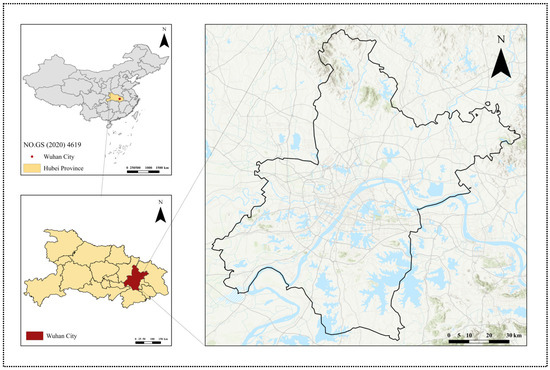
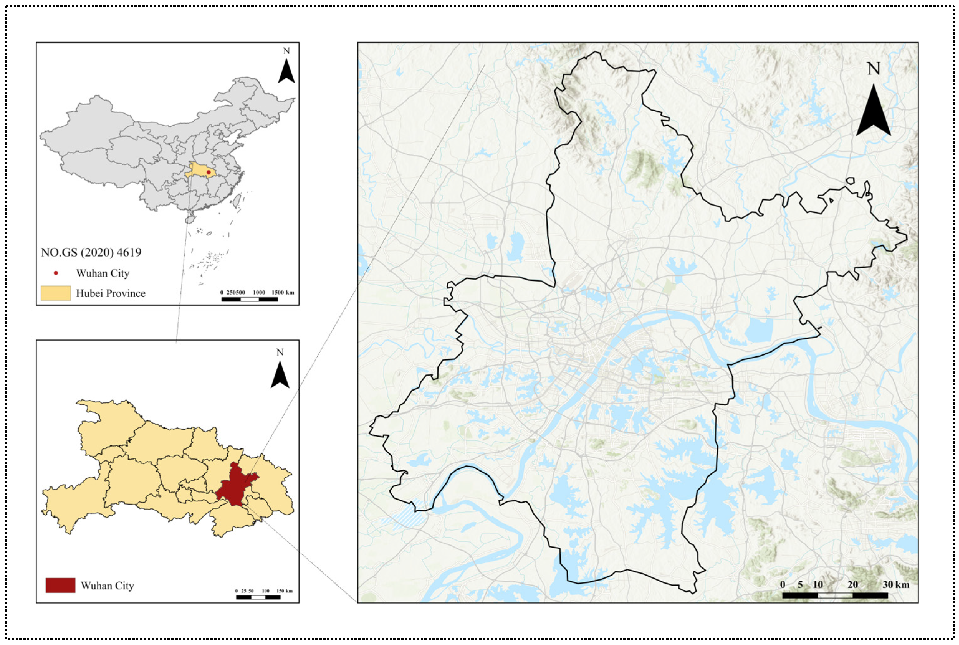
Wuhan (113°41′ E–115°05′ E, 29°58′ N–31°22′ N) is located in the eastern part of the Jianghan Plain, where the Yangtze River and the Han River converge. This region has a typical subtropical monsoon climate, with four distinct seasons and abundant rainfall. In summer, influenced by the Western Pacific Subtropical High, southerly winds prevail, atmospheric convection is strong, and pollutants can be easily dispersed. In contrast, during winter and spring, under the combined influence of cold air from the north and local temperature inversions, northerly winds prevail, facilitating regional pollutant accumulation and cross-border transport. The geographical location of Wuhan is shown in Figure 1.
Figure 1.
Geographical location of Wuhan.
2.2. Data Sources and Data Preprocessing
The dataset used in this study spanned from 1 January 2016 to 31 December 2025, with a daily temporal resolution. Air quality monitoring data were obtained from the China Air Quality Historical Data Platform (https://www.aqistudy.cn/historydata/, accessed on 20 February 2026). The collected indicators included daily PM2.5 concentration (target variable, μg/m3) as well as co-pollutant variables SO2 (μg/m3), NO2 (μg/m3), CO (mg/m3) and O3 (μg/m3).
Meteorological data were obtained from the ERA5 global atmospheric reanalysis dataset [37] released by the European Centre for Medium-Range Weather Forecasts (ECMWF) (https://cds.climate.copernicus.eu/datasets/reanalysis-era5-single-levels, accessed on 20 February 2026). The study first downloaded hourly gridded meteorological data covering Wuhan, performed spatial masking and clipping based on the city boundary, and calculated the mean value of all grid cells within the study area to obtain meteorological time series representing the overall characteristics of the city. Subsequently, temporal aggregation was performed to generate daily-scale meteorological variables: daily average temperature (Temp), relative humidity (RH), average wind speed (WS), and pressure (Pres) were calculated as 24-h mean values, while precipitation (Prec) was calculated as the 24-h cumulative amount. This process generated daily meteorological variables and ensured spatiotemporal consistency with the air quality monitoring data. The target variable, air pollutant variables, and meteorological variables used in this study are listed in Table 1. All predictor variables were constructed using observations from the same day as the target PM2.5 concentration. Time-lagged variables were not included in order to maintain model interpretability and facilitate subsequent SHAP-based attribution analysis of the direct relationships between environmental factors and PM2.5 concentration.
Table 1.
Description of Variables Used in This Study.
To improve data quality and reduce the impact of abnormal samples on model training, the raw data were first subjected to missing value imputation, outlier identification, and time-series alignment. For a small number of missing data points, the mean of adjacent time steps was used for imputation. Outlier identification was performed using the 3σ principle: a sample was identified as an outlier if its value fell outside the range of mean ± 3 standard deviations and was then replaced by the mean of adjacent time periods. Subsequently, all variables were aligned according to the time series to ensure data integrity and temporal consistency.
Since air pollutant concentrations and meteorological variables have different scales and numerical ranges, all input variables were normalized using the Min–Max method before model training. The variables were mapped to the [0, 1] interval to reduce the influence of feature scale differences and improve training efficiency and convergence stability.
2.3. Machine Learning Models
2.3.1. Tree-Based Machine Learning Models
This study selected four tree-based machine learning models—Decision Tree (DT), Random Forest (RF), XGBoost, and LightGBM—for PM2.5 concentration estimation.
Decision Tree (DT) is a supervised learning method based on recursive feature partitioning. It achieves regression of the target variable by repeatedly selecting the optimal features to partition the sample space [38]. In regression tasks, the decision tree typically uses the principle of minimizing squared error to determine the optimal split point, and its objective function can be expressed as:
where yi and ŷi represent the actual and estimated values, respectively.
Random Forest (RF) is an ensemble learning model based on decision trees. It generates multiple training subsets through Bootstrap random sampling and constructs multiple decision trees for ensemble learning, thereby improving model stability and reducing the risk of overfitting [39].
XGBoost is an ensemble learning algorithm based on gradient boosting. It iteratively builds weak learners and continuously optimizes residuals to enhance model performance [40]. Compared with traditional boosting tree models, XGBoost offers advantages in regularization control and computational efficiency.
LightGBM is also a gradient boosting decision tree model. It employs a histogram-based feature splitting strategy and a leaf-wise growth approach, which improve training efficiency and reduce memory consumption [41].
2.3.2. Support Vector Machine
Support Vector Machine (SVM) is a supervised learning method based on statistical learning theory. In regression tasks, Support Vector Regression (SVR) is typically used to perform nonlinear regression. SVM maps input features into a high-dimensional space using a kernel function and constructs an optimal regression hyperplane in that space, thereby improving the model’s ability to represent complex nonlinear relationships [42].
The regression function can be expressed as:
where ϕ(x), w and b represent the kernel mapping function, weight vector, and bias term, respectively.
Due to its strong generalization ability and capability to model nonlinear relationships, SVM is widely used in air quality modeling studies [43].
2.3.3. Multilayer Perceptron
The Multilayer Perceptron (MLP) is a typical feedforward artificial neural network, consisting of an input layer, hidden layers, and an output layer. Through multi-layer nonlinear mapping, the MLP can effectively learn complex relationships between input variables and target variables, making it suitable for modeling air quality data [44].
During the training process, neurons in the hidden layers perform nonlinear transformations of the input features to generate outputs. The computation process can be expressed as:
where xi, wi, b and f represent the input feature, connection weight, bias term, and activation function, respectively.
In this study, the MLP model was used to estimate PM2.5 concentration, and the PSO algorithm was employed to optimize its hyperparameters, thereby improving model performance.
2.3.4. Particle Swarm Optimization Algorithm
Particle Swarm Optimization (PSO) is a global optimization algorithm based on the concept of swarm intelligence. It performs optimization in the parameter space by simulating the cooperative search process of a particle swarm [45].
In the PSO algorithm, the position of each particle represents a set of parameters to be optimized. Particles perform a global search by continuously updating their velocity and position. The update process is as follows:
where denotes the particle velocity, denotes the particle position, and denote the personal best position and global best position, respectively, w denotes the inertia weight, and c1 and c2 denote the learning factors.
In this study, the PSO algorithm was used to optimize the hyperparameters of each machine learning model, aiming to improve estimation accuracy and generalization ability.
2.3.5. SHAP Interpretability Analysis Method
To improve the interpretability of machine learning models, this study employed the SHAP (Shapley Additive Explanations) method to analyze the contributions of different input variables to PM2.5 estimation results [46,47].
The SHAP method is based on Shapley value theory. It provides global and local interpretation of complex models by calculating the marginal contribution of each input variable to the model output. The calculation formula is as follows:
where ϕi denotes the SHAP value of feature i, F denotes the set of all features, and S denotes a feature subset.
In this study, SHAP global importance analysis, beeswarm plots, heatmaps, and dependence plots were combined to analyze the contributions of different variables to PM2.5 estimation.
2.4. Evaluation Metrics
To comprehensively evaluate the performance of each PSO-optimized machine learning model for PM2.5 concentration estimation, this study adopted three evaluation metrics: Root Mean Square Error (RMSE), Mean Absolute Error (MAE), and the coefficient of determination (R2). These metrics evaluate model performance from different perspectives, including estimation error, absolute deviation, and overall goodness of fit, thereby providing a comprehensive assessment of estimation performance. The calculation formulas for each evaluation metric are as follows:
where yi, ŷi, and n represent the actual PM2.5 concentration, the estimated value output by the model, and the number of samples, respectively. Smaller RMSE and MAE values indicate better model performance. The coefficient of determination R2 ranges from 0 to 1; values closer to 1 indicate better goodness of fit and higher estimation accuracy.
3. Results
3.1. Exploratory Analysis
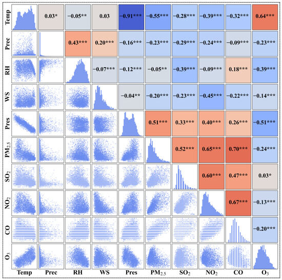
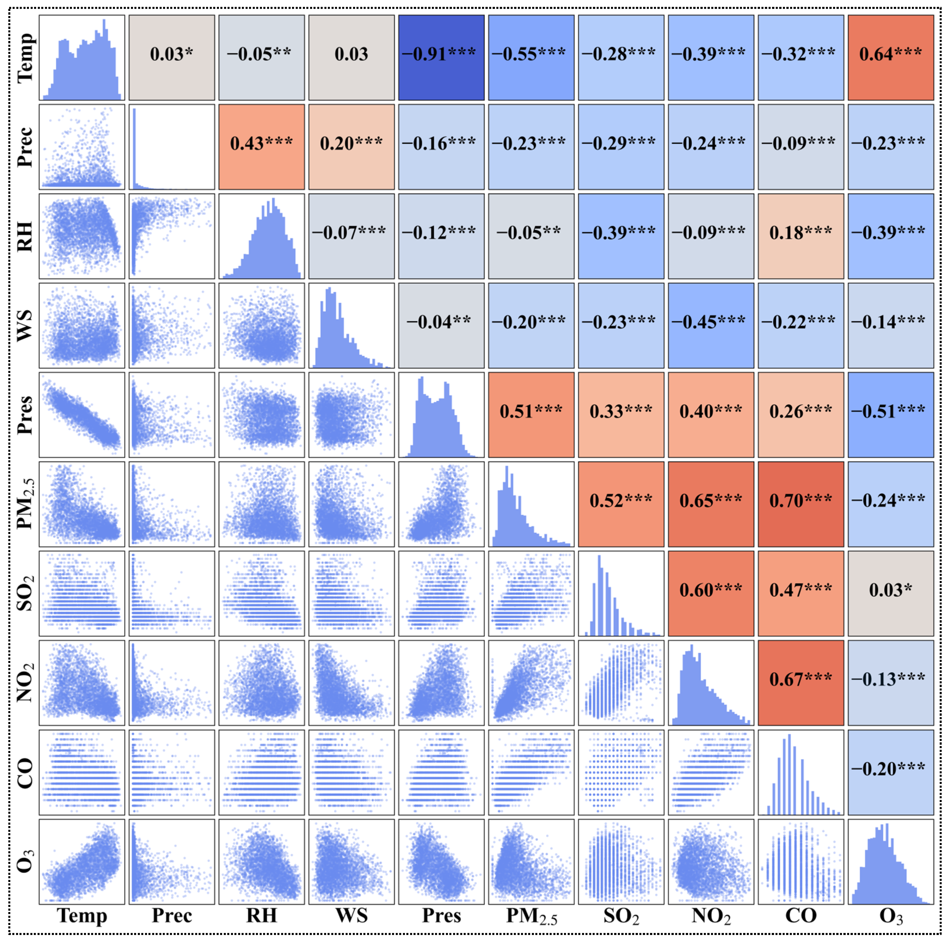
In atmospheric environmental data monitoring and modeling, systematically analyzing the association between each feature variable and the target variable is a prerequisite. It helps evaluate the effectiveness of feature engineering and understand the basic characteristics of the data. To explore the relationships between PM2.5 concentrations and meteorological factors as well as co-pollutants in Wuhan, this study conducted exploratory data analysis based on daily data from 2016 to 2025 (Figure 2). The upper triangular region of the figure shows the Spearman correlation coefficients (r) and their significance levels between variables [48]. The lower triangular region illustrates the pairwise relationship patterns between variables through scatter plots. The diagonal shows the frequency distribution of each variable. Together, these visualizations provide a comprehensive overview of the correlations, relationship patterns, and statistical distributions of the variables.
Figure 2.
Variable Distribution and Correlation Matrix. (Note: *, **, and *** indicate statistical significance at the p < 0.05, p < 0.01, and p < 0.001 levels, respectively).
In terms of variable distribution, air pressure (Pres), temperature (Temp), and ozone (O3) generally exhibit wide value ranges. Among them, Temp and O3 exhibit bimodal distributions, reflecting significant seasonal variations in Wuhan. Precipitation (Prec), wind speed (WS), as well as CO, NO2, and SO2, show a clear right-skewed distribution. Most observations are concentrated in the lower range, with only a few samples showing high values. PM2.5 concentration also exhibits a typical right-skewed distribution, indicating that high-concentration pollution events occur relatively infrequently, whereas PM2.5 levels remain at low or moderate levels during most periods.
Regarding the relationships among variables, most air pollutants exhibit strong linear relationships with PM2.5. Among the meteorological factors, Prec and Temp show relatively high degrees of linear association with PM2.5, whereas the remaining factors exhibit more complex relationships with PM2.5. Further Spearman correlation analysis results indicate that PM2.5 has a strong positive correlation with CO (r = −0.7, p < 0.001) and NO2 (r = −0.65, p < 0.001), suggesting that different pollution indicators exhibit significant temporal synchrony. Among them, CO and NO2 are commonly regarded as indicators of urban traffic activity and overall pollution levels. Their strong correlations with PM2.5 suggest that PM2.5 levels are closely associated with urban pollution accumulation processes.
Among the meteorological factors, wind speed (WS) and precipitation (Prec) are generally negatively correlated with PM2.5. The correlation coefficient between WS and PM2.5 is −0.20 (p < 0.01), and that between Prec and PM2.5 is −0.23 (p < 0.01), indicating that stronger atmospheric diffusion conditions and precipitation processes typically correspond to lower PM2.5 concentrations. Temperature (Temp) and pressure (Pres) also show noticeable correlations with PM2.5, suggesting that meteorological conditions may influence PM2.5 concentration variations.
Furthermore, the correlation between relative humidity (RH) and PM2.5 is relatively weak (r = −0.05, p < 0.01), suggesting a potentially complex nonlinear relationship between the two.
3.2. PSO Hyperparameter Optimization and Model Performance Comparison
To improve the estimation performance of each machine learning model, this study employed the Particle Swarm Optimization (PSO) algorithm to optimize model hyperparameters. The PSO algorithm iteratively searched the parameter space to identify the optimal hyperparameter combination for each model.
Given the temporal characteristics of air quality and meteorological data, the experiment adopted a time series-based split into training and test sets [49], without randomly shuffling the samples. The first 80% of the time-series data was used as the training set for model construction, and the remaining 20% was used as the test set for model performance evaluation, thereby preventing future temporal information leakage from affecting the results.
To enhance model training stability and reduce the risk of overfitting, this study optimized model parameters using a five-fold cross-validation method based on time series rolling windows (Time Series Split). In each round of training, the model was trained on historical time-series data and validated on the subsequent time window, ensuring that the evaluation process reflects the real-world scenario of time-series estimation tasks. All experiments were conducted on the Windows 11 operating system, with an Intel Core i7-12700H CPU and 16 GB RAM. Model training and analysis were implemented using Python 3.11.
Based on previous studies [50] and preliminary experiments, the PSO parameters were set as follows. The particle swarm size was 30, and the maximum number of iterations was 100. The inertia weight was set to 0.7, and both the cognitive and social learning factors were set to 1.5. The convergence threshold was set to 1 × 10⁻⁶. The RMSE obtained during cross-validation was used as the objective function to be minimized. When the improvement in the objective function was less than 1 × 10⁻⁶ over 10 consecutive iterations, the algorithm was considered to have met the convergence condition, and the search process was terminated early.
Table 2 presents the optimal hyperparameter combinations and computational efficiency results for each model after PSO. The models exhibited notable differences during the parameter search process. Among them, the DT model converged the fastest, while the MLP model required relatively higher training time due to its complex network structure. Overall, the PSO algorithm effectively explored the parameter space and identified optimal hyperparameter configurations for different models.
Table 2.
Hyperparameters and computational efficiency of six machine learning models optimized by the PSO algorithm.
To evaluate the impact of PSO on model performance, this study further compared the performance of each model before and after optimization. The results are shown in Table 3. Overall, PSO improved the performance of all six machine learning models. This was reflected in higher R2 values and lower RMSE and MAE values. These results indicate that PSO effectively identified improved hyperparameter combinations, thereby enhancing estimation performance and generalization ability.
Table 3.
Performance comparison before and after PSO.
Among them, the decision tree (DT) model showed the greatest improvement. Its R2 increased from 0.3535 to 0.6423, an increase of 81.70%. At the same time, RMSE and MAE decreased by 25.62% and 30.57%, respectively. This suggests that appropriate hyperparameter settings can substantially improve the estimation performance of a single decision tree model. Ensemble learning models such as random forest (RF), XGBoost, and LightGBM also showed consistent performance improvements. Their R2 values increased to 0.6962, 0.7182, and 0.7215, respectively, accompanied by corresponding reductions in RMSE and MAE. This indicates that PSO can further enhance the performance of ensemble learning models.
In addition, the SVM and MLP models showed better estimation performance after optimization. The R2 of the SVM model increased from 0.6024 to 0.7451, while its RMSE decreased from 15.8421 to 12.6693, a reduction of 20.03%. This indicates that the SVM model is relatively sensitive to hyperparameter settings. After optimization, the MLP model achieved the highest coefficient of determination (R2 = 0.7465) among all models, with RMSE and MAE reduced to 12.6356 and 8.8582, respectively. This suggests that appropriate hyperparameter tuning can effectively enhance the capability of neural networks to learn complex nonlinear relationships.
Overall, PSO had a positive effect on all models. It not only improved model performance but also reduced estimation errors. Among them, parameter-sensitive models such as SVM and MLP showed greater performance improvements, further demonstrating the effectiveness of PSO for hyperparameter optimization in machine learning models.
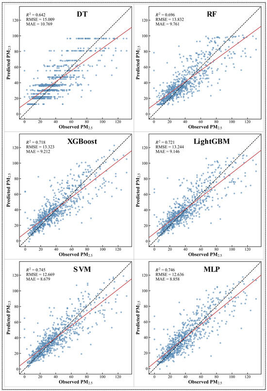
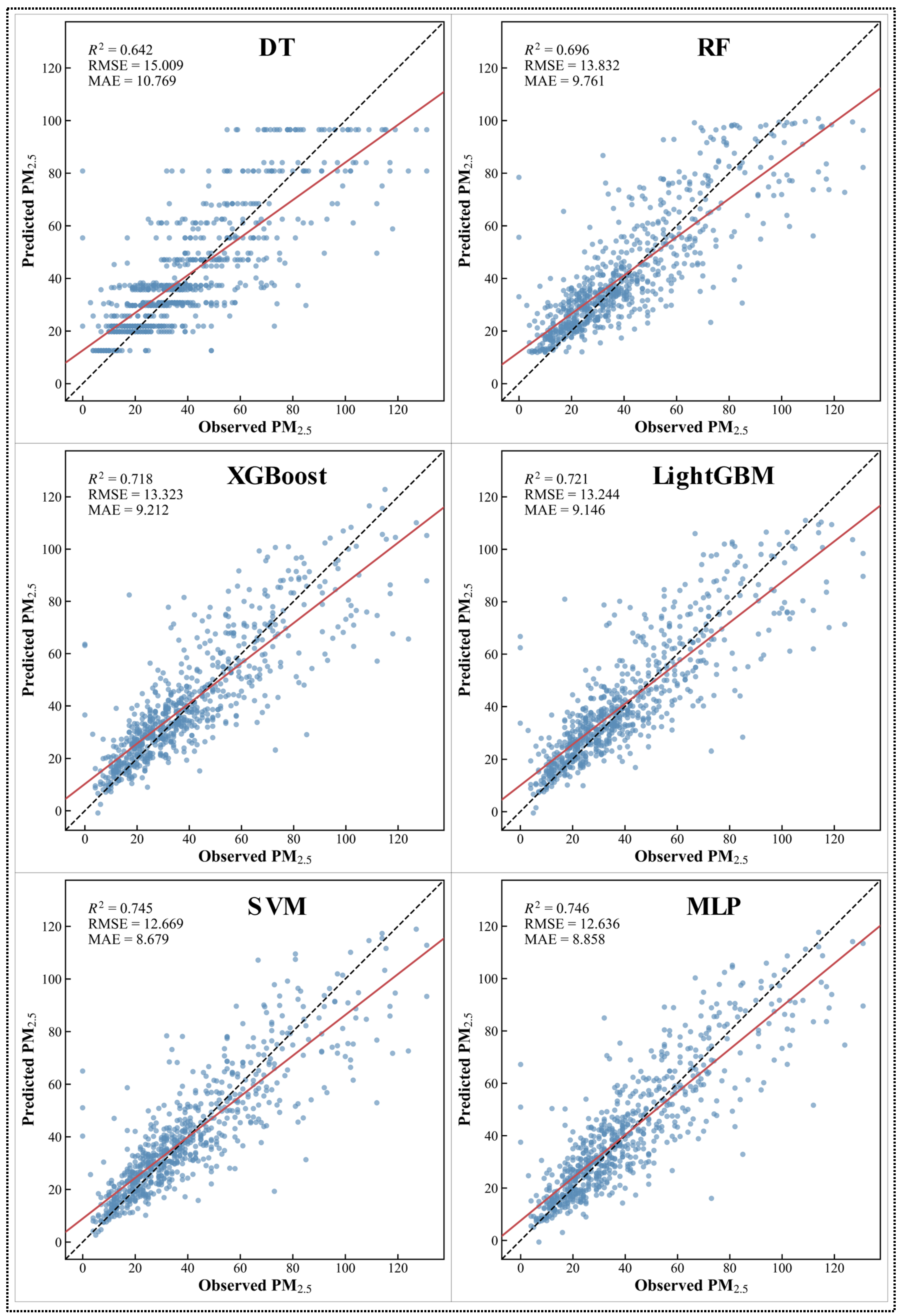
To further compare the performance of different models for PM2.5 concentration estimation, this study evaluated the performance of each model using an independent test set. The scatter plots of observed versus estimated values are shown in Figure 3.
Figure 3.
Scatter plots of estimated versus observed values for six machine learning models on the independent test set. (Note: The black dashed line represents the 1:1 line, and the red solid line represents the linear regression line).
Based on the R2, RMSE, and MAE results shown in Figure 3, the estimation performance of the models differed substantially on the test set.
Among them, the Decision Tree (DT) model showed relatively weak estimation performance, with an R2 of only 0.642 on the test set, and RMSE and MAE reaching 15.009 μg/m3 and 10.769 μg/m3, respectively. The scatter points were widely dispersed, suggesting that a single decision tree has limitations when handling continuously changing air quality data.
In contrast, the ensemble learning models (RF, XGBoost, LightGBM) showed improved estimation performance. The RF model achieves an R2 of 0.696 on the test set, while XGBoost and LightGBM achieve R2 values of 0.718 and 0.721, respectively, with scatter points gradually approaching the 1:1 reference line. This indicates that ensemble learning methods can better capture PM2.5 concentration dynamics.
Furthermore, the SVM and MLP models demonstrated superior estimation performance on the test set. The SVM model achieved a relatively low MAE (8.679 μg/m3), indicating good stability. Among all models, the PSO-MLP achieved the best overall performance, with an R2 of 0.746 on the test set, and RMSE and MAE reduced to 12.636 μg/m3 and 8.858 μg/m3, respectively. Its scatter points were closest to the 1:1 reference line.
The results indicate that, compared with the interval-based partitioning strategy of tree-based models, the MLP model can better learn the complex nonlinear relationships between input variables and PM2.5 concentration through multi-layer nonlinear mapping [24,51], thus achieving superior estimation performance on the dataset used in this study.
Based on the comprehensive evaluation results, PSO-MLP was identified as the optimal estimation model and was subsequently used for SHAP analysis.
3.3. SHAP-Based Global Interpretation and Seasonal Dynamic Analysis of PM2.5 Estimation
To improve the interpretability of the neural network model, the SHAP method was applied to the optimal PSO-MLP model to quantify the contributions of individual input variables to PM2.5 estimation.
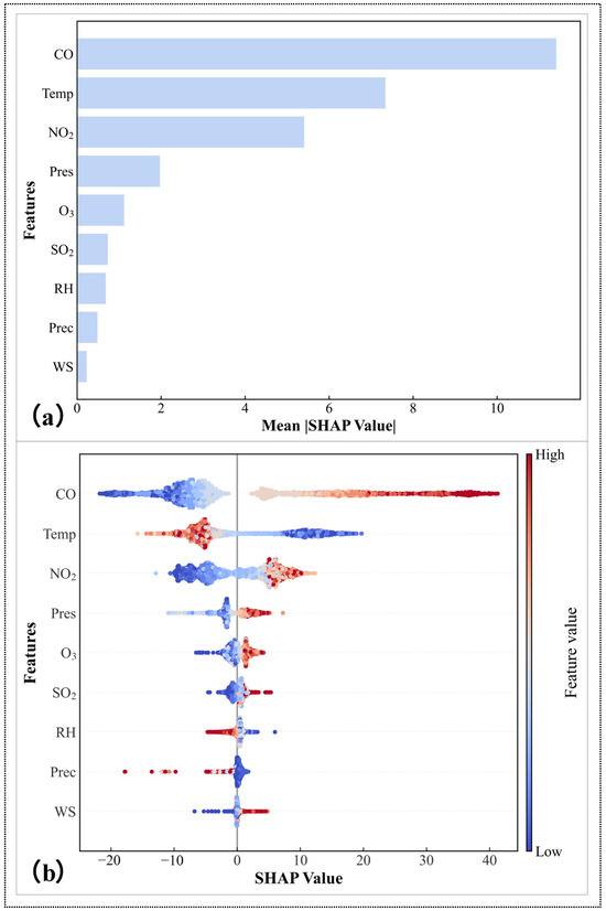
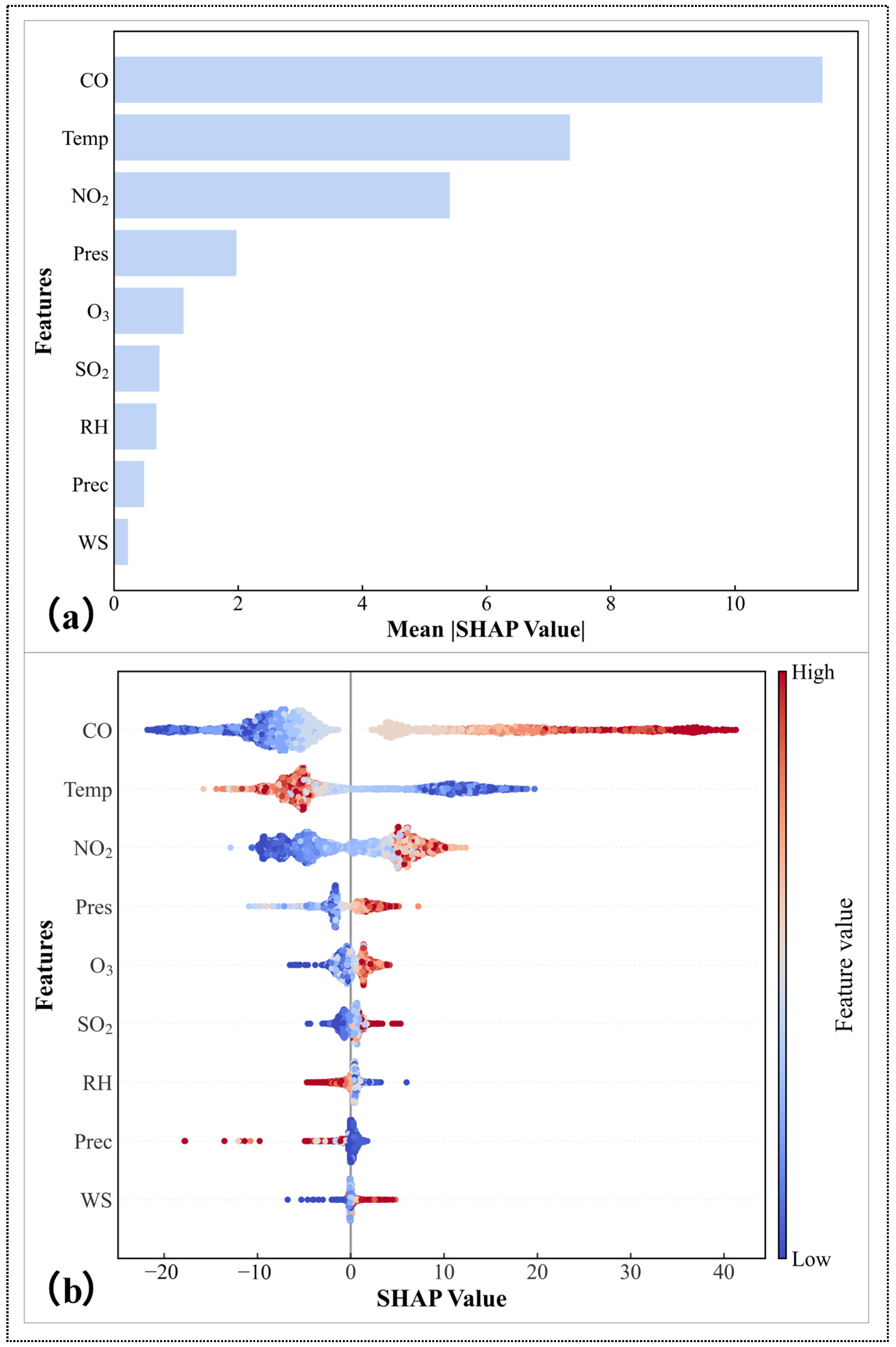
Figure 4a presents the global feature importance ranking based on the mean absolute SHAP values. There were substantial differences in the contributions of different input variables to PM2.5 estimation. Among them, CO showed the highest importance, with a mean absolute SHAP value of 11.4, indicating the largest contribution to model outputs. Temp and NO2 ranked second and third, with values of 7.3 and 5.4, respectively, suggesting that both meteorological conditions and air pollutants jointly influence PM2.5 concentrations. In contrast, variables such as SO2, RH, Prec, and WS have relatively lower importance and contribute less to the model’s overall performance.
Figure 4.
Global SHAP interpretation results of the PSO-MLP model. (a) Mean absolute SHAP value ranking of input features; (b) SHAP beeswarm distribution of feature contributions.
Figure 4b further illustrates the SHAP value distributions of different variables across all samples. The results show that each variable exhibited a clear nonlinear relationship with PM2.5 estimation. Among them, high values of CO and NO2 were generally associated with larger positive SHAP values, indicating that elevated CO and NO2 levels were associated with higher estimated PM2.5 concentrations. In contrast, high temperatures were generally associated with lower SHAP values, whereas lower temperatures tended to produce larger positive SHAP contributions, suggesting that temperature plays an important role in PM2.5 estimation. Additionally, wind speed (WS) and precipitation (Prec) generally exhibited negative SHAP contributions, meaning that higher wind speed and precipitation conditions are typically associated with lower PM2.5 estimation.
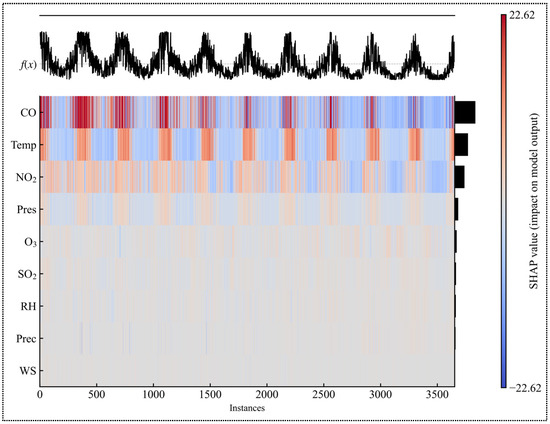
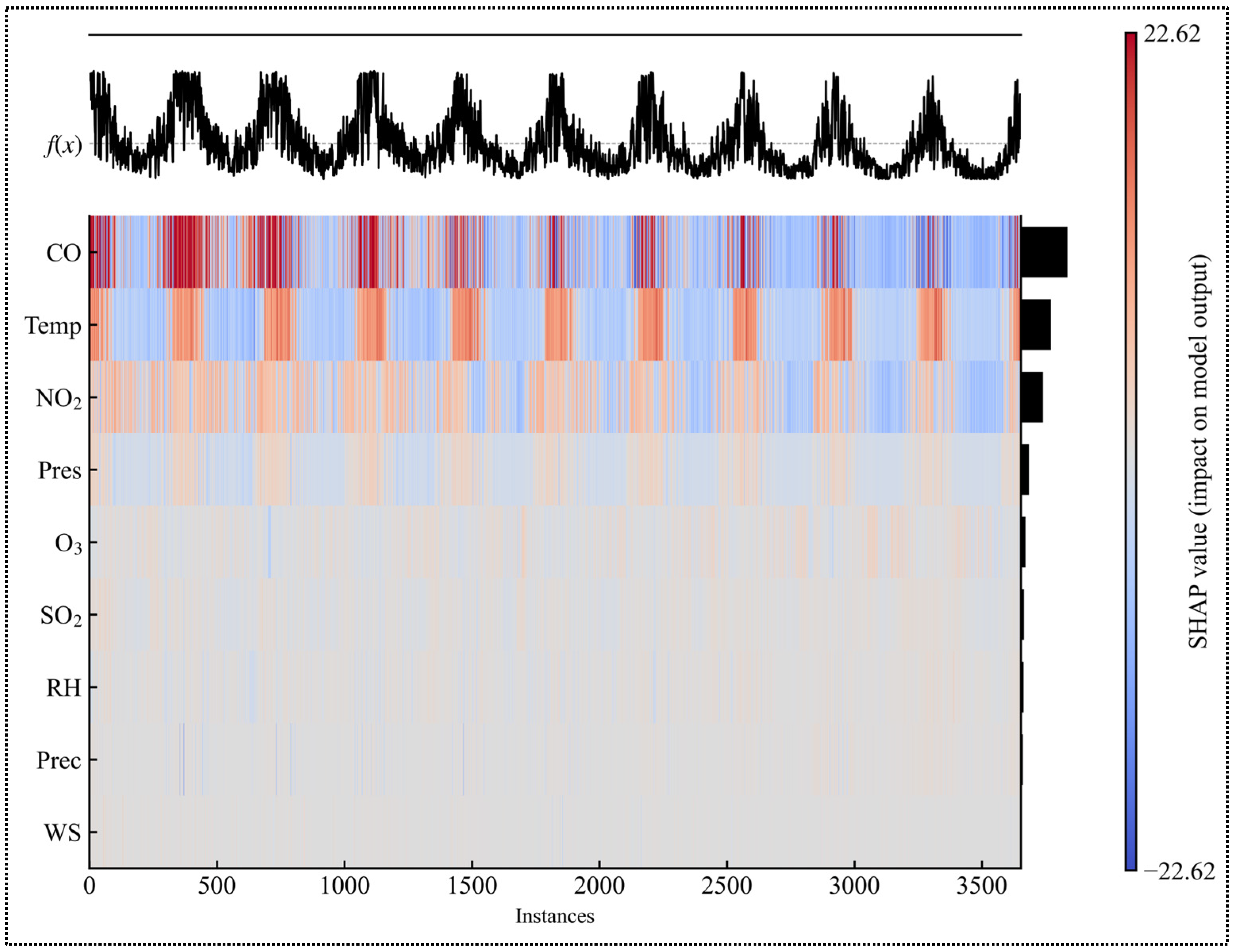
To further analyze the temporal dynamic of different influencing factors, a long-term SHAP heatmap for the period 2016–2025 was generated, as shown in Figure 5. The results indicate that PM2.5 estimates exhibit a clear seasonal pattern, generally following a “higher in winter and lower in summer” trend.
Figure 5.
Seasonal SHAP heatmap of different influencing factors from 2016 to 2025.
The SHAP values of Temp exhibit a clear seasonal pattern, with contributions fluctuating regularly across seasons. CO and NO2 generally exhibit higher SHAP contributions during winter, coinciding with periods of elevated PM2.5 concentrations. This indicates that the effects of air pollutants and meteorological conditions on PM2.5 estimates vary over time. Overall, the contributions of different variables to PM2.5 estimates exhibit substantial temporal variability.
3.4. Nonlinear Response Characteristics of Different Influencing Factors Based on SHAP Dependence Analysis
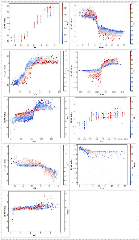
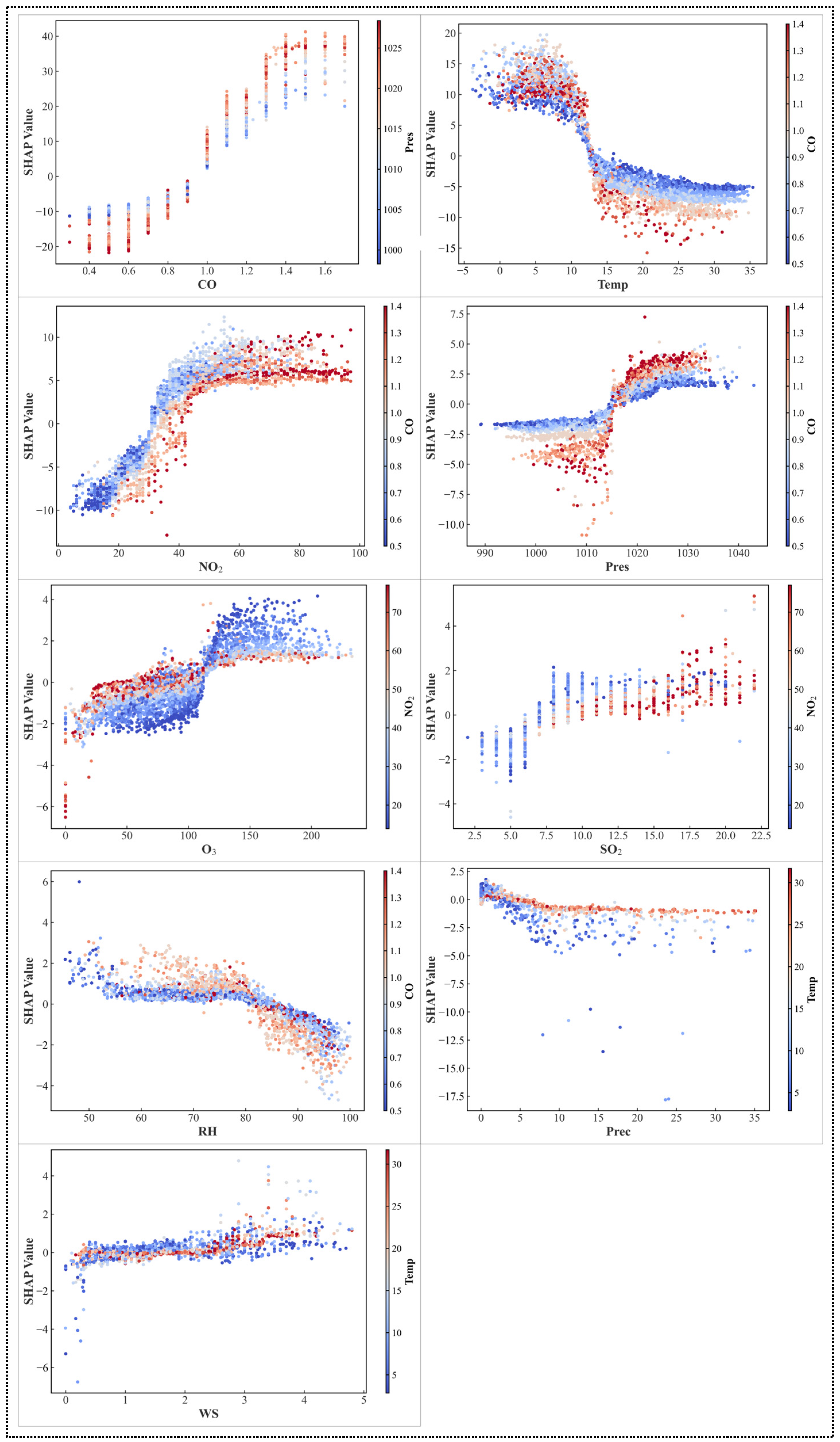
To further investigate the nonlinear relationships between input variables and PM2.5 estimates, SHAP dependence plots were used to analyze the local effects of individual variables. The results are shown in Figure 6.
Figure 6.
SHAP dependence plots of different influencing factors for PM2.5 estimation.
Overall, each variable exhibits a clear nonlinear relationship with PM2.5 estimation. Higher values of CO and NO2 generally correspond to larger positive SHAP contributions, indicating a relatively strong association between high values of these pollution indicators and higher PM2.5 estimation. This result is generally consistent with findings from existing air quality studies, which have concluded that CO, NO2, and meteorological conditions play important roles in influencing changes in PM2.5 concentration [48]. In contrast, SO2 exhibits relatively small SHAP contributions, suggesting a weaker influence on model estimation than the other pollution indicators.
Meteorological factors also exhibit complex nonlinear relationships with PM2.5 estimation. Among them, Temp exhibits a distinct threshold-like response pattern with respect to PM2.5 estimation. Low-temperature conditions generally correspond to higher positive SHAP contributions, while as temperature increases, the SHAP values tend to decline. Higher Pres values are associated with larger positive SHAP contributions, indicating that model estimation values are generally higher under high-pressure conditions.
Additionally, as precipitation (Prec) and wind speed (WS) increase, the SHAP values show an overall decreasing trend, indicating that stronger atmospheric dispersion and precipitation conditions are generally associated with lower PM2.5 estimation. Relative humidity (RH) exhibits a more complex nonlinear pattern, with its SHAP contribution fluctuating across different humidity ranges.
4. Discussion
4.1. Driving Mechanisms of Major Environmental Factors on PM2.5 Concentration
SHAP analysis results indicate that CO, Temp, and NO2 are the primary factors influencing PM2.5 concentration in Wuhan. CO and NO2 rank high in feature importance, indicating that anthropogenic emission processes play an important role in PM2.5 concentration changes. Both CO and NO2 mainly originate from vehicle exhaust emissions, industrial combustion, and fossil fuel consumption. Therefore, they can serve as indicators of urban anthropogenic activity and pollution emission intensity [52]. In addition, as important precursors of atmospheric photochemical reactions, NO2 can also participate in the formation of secondary aerosols such as nitrates, thereby contributing to increased PM2.5 concentrations [53].
Temperature is the second most important influencing factor after CO. Its SHAP results show that higher temperatures generally correspond to lower PM2.5 concentrations. This phenomenon may be related to changes in boundary-layer structure and enhanced atmospheric dispersion. Under higher-temperature conditions, atmospheric convection activity intensifies and the boundary layer height increases, which facilitates the vertical diffusion and dilution of pollutants. In contrast, lower temperatures are more likely to create stagnant weather and temperature inversions, leading to the accumulation of pollutants [54].
Wind speed and precipitation generally show negative contributions. Higher wind speed can enhance the horizontal transport and vertical diffusion of pollutants, reducing the accumulation of pollutants near the surface. Precipitation can effectively remove atmospheric particulate matter through wet deposition, and therefore typically corresponds to lower PM2.5 concentrations [55]. In contrast, relative humidity exhibits a more complex nonlinear relationship with PM2.5. Its effects may result from multiple interacting processes, including hygroscopic growth of particles, changes in the boundary layer, and secondary aerosol formation [56].
4.2. Temporal Dynamics of Environmental Drivers and Seasonal Variability
The SHAP heatmap shows clear seasonal variations in the contributions of different environmental factors to PM2.5 concentrations, generally presenting a pattern of “higher in winter and lower in summer”. Among them, CO and NO2 exhibit higher positive contributions during winter and coincide with periods of elevated PM2.5 concentrations.
This phenomenon may be closely related to unfavorable meteorological conditions and the pollutant accumulation effect in winter. In winter, the boundary layer height decreases, the atmospheric stratification becomes stable, and near-surface diffusion conditions deteriorate. At the same time, the frequency of stagnant weather and temperature inversions increases, making it easier for pollutants to accumulate near the surface [57]. In addition, the enhanced regional transport effect and the cumulative effect of anthropogenic emissions in winter jointly contribute to elevated PM2.5 concentrations, leading to a significant increase in the contribution of CO and NO2 to model estimation [58].
In contrast, high temperatures, strong convection, and frequent precipitation processes in summer facilitate pollutant diffusion and removal. Consequently, PM2.5 concentrations are generally lower, and the SHAP contributions of the driving factors are correspondingly reduced [55]. These results indicate that PM2.5 concentrations are influenced not only by emission intensity but also by meteorological conditions and regional transport processes.
4.3. Limitations and Future Perspectives
Although the PSO-optimized machine learning framework achieved satisfactory performance in PM2.5 estimation and driving-factor analysis, several limitations remain. To maintain model interpretability, this study did not incorporate time-lagged features or temporal deep learning models such as LSTM and Transformer, which may limit the exploitation of temporal dependencies in PM2.5 variations. In addition, the meteorological variables were derived from the ERA5 reanalysis dataset, which may introduce uncertainties compared with ground-based observations. In addition, this study primarily considered routinely available air quality and meteorological variables. Although these variables capture the major atmospheric conditions associated with PM2.5 variability, other important influencing factors—such as emission intensity variations [59], regional transport processes [60], land-use characteristics [61], and socioeconomic activities [62]—were not explicitly included due to data availability and scale consistency constraints. These factors are known to play important roles in shaping urban air pollution patterns, and their absence may limit the completeness of mechanistic interpretation in this study. Future studies could integrate multi-source environmental data and socioeconomic datasets, including satellite-derived aerosol optical depth (AOD) products, emission inventories, land-use information, and human activity indicators, and explore the combination of temporal deep learning models, graph neural networks (GNNs), and explainable artificial intelligence methods. In addition, transfer learning strategies could be investigated to improve model generalization and adaptability across different regions.
5. Conclusions
Based on daily air quality and meteorological data from Wuhan during 2016–2025, this study constructed six machine learning models—Decision Tree (DT), Random Forest (RF), XGBoost, LightGBM, Support Vector Machine (SVM), and Multilayer Perceptron (MLP)—and optimized their hyperparameters using the Particle Swarm Optimization (PSO) algorithm. On this basis, the SHAP method was used to perform an interpretability analysis on the optimal model. The main conclusions are as follows:
- (1)
- Different machine learning models exhibited substantial differences in predictive performance in the task of PM2.5 concentration estimation. Among them, the PSO-MLP model achieved the best overall performance, with a coefficient of determination (R2) of 0.746 on the test set and root mean square error (RMSE) and mean absolute error (MAE) values reducing to 12.636 μg/m3 and 8.858 μg/m3, respectively, demonstrating strong predictive performance and generalization capability.
- (2)
- The global interpretation results of SHAP indicate that the contributions of different input variables to PM2.5 estimation vary significantly. Among them, CO, Temp, and NO2 showed relatively high importance, whereas variables such as SO2, RH, and WS contributed less to model outputs. This suggests that both air pollution indicators and meteorological conditions jointly influence PM2.5 concentrations.
- (3)
- The SHAP heatmap analysis showed that the contributions of different variables to PM2.5 estimation exhibited clear seasonal variations. Among them, Temp demonstrates a pronounced periodic pattern, while CO and NO2 generally exhibited higher contributions during winter.
- (4)
- The SHAP dependence analysis results indicate that each influencing factor exhibited a clear nonlinear relationship with PM2.5 estimation. Among them, CO and NO2 in their higher value ranges were generally associated with higher SHAP contributions, while as wind speed and precipitation increased, the SHAP values showed an overall decreasing trend.
Overall, machine learning models optimized by PSO effectively improved the predictive performance of PM2.5 concentration models, and SHAP provides valuable insights into the behavior of complex machine learning models. Future work may further integrate remote sensing data, multi-region transfer learning, and long-term time series data to enhance model generalizability and applicability across different regions.
Author Contributions
Conceptualization, Q.L. and J.F.; methodology, Q.L.; software, Q.L.; validation, Q.L. and J.F.; formal analysis, Q.L.; investigation, J.F.; resources, Q.L.; data curation, Q.L.; writing—original draft preparation, Q.L.; writing—review and editing, Q.L. and J.F.; visualization, Q.L.; supervision, J.F.; project administration, J.F.; funding acquisition, J.F. All authors have read and agreed to the published version of the manuscript.
Funding
This research was funded by the National Natural Science Foundation of China, grant number 42171413.
Data Availability Statement
The data used in this study are all derived from public domain resources: Air quality data were obtained from the China Air Quality Historical Data Platform (https://www.aqistudy.cn/historydata/ (accessed on 25 February 2026)). Meteorological data were obtained from the ERA5 global atmospheric reanalysis dataset provided by the European Centre for Medium-Range Weather Forecasts (ECMWF) (https://cds.climate.copernicus.eu/datasets/reanalysis-era5-single-levels (accessed on 26 February 2026)). The processed meteorological data derived from the above original data by our team are not publicly available temporarily, and can be obtained from the corresponding author upon reasonable request.
Acknowledgments
We would like to thank the editors and reviewers for their constructive comments and suggestions.
Conflicts of Interest
The authors declare no conflicts of interest.
Abbreviations
Since some parts of this article are abbreviated, a table explaining what each abbreviation means has been inserted to further enhance the readability of the article.
| DT | Decision Tree |
| RF | Random Forest |
| XGBoost | Extreme Gradient Boosting |
| LightGBM | Light Gradient Boosting Machine |
| SVM | Support Vector Machine |
| MLP | Multilayer Perceptron |
| PSO | Particle Swarm Optimization |
| SHAP | Shapley Additive Explanations |
| RMSE | Root Mean Square Error |
| MAE | Mean Absolute Error |
| R2 | Coefficient of Determination |
References
- Akhtar, N.; Han, J.-Y. Machine Learning–Driven Reclassification of Air Quality Zones and PM2.5 Prediction: A Case Study in a Subtropical Region. Urban Clim. 2026, 65, 102766. [Google Scholar] [CrossRef] [Scilit]
- Ni, Q.; Wang, Y.; Yuan, J. Adaptive Scalable Spatio-Temporal Graph Convolutional Network for PM2.5 Prediction. Eng. Appl. Artif. Intell. 2023, 126, 107080. [Google Scholar] [CrossRef] [Scilit]
- Choi, S.-M.; Choi, H. Statistical Modeling for PM10, PM2.5 and PM1 at Gangneung Affected by Local Meteorological Variables and PM10 and PM2.5 at Beijing for Non- and Dust Periods. Appl. Sci. 2021, 11, 11958. [Google Scholar] [CrossRef] [Scilit]
- Kim, S.-M.; Koo, J.-H.; Lee, H.; Mok, J.; Choi, M.; Go, S.; Lee, S.; Cho, Y.; Hong, J.; Seo, S.; et al. Comparison of PM2.5 in Seoul, Korea Estimated from the Various Ground-Based and Satellite AOD. Appl. Sci. 2021, 11, 10755. [Google Scholar] [CrossRef] [Scilit]
- Yin, P.-Y.; Chang, R.-I.; Day, R.-F.; Lin, Y.-C.; Hu, C.-Y. Improving PM2.5 Concentration Forecast with the Identification of Temperature Inversion. Appl. Sci. 2021, 12, 71. [Google Scholar] [CrossRef] [Scilit]
- Xu, W.; Fu, F.; Zhang, Q.; Wang, L. A Deep Learning-Based Multi-Objective Optimization Model for PM2.5 Prediction. Int. J. Comput. Intell. Syst. 2023, 16, 141. [Google Scholar] [CrossRef] [Scilit]
- Wu, F.; Min, P.; Jin, Y.; Zhang, K.; Liu, H.; Zhao, J.; Li, D. A Novel Hybrid Model for Hourly PM2.5 Prediction Considering Air Pollution Factors, Meteorological Parameters and GNSS-ZTD. Environ. Model. Softw. 2023, 167, 105780. [Google Scholar] [CrossRef] [Scilit]
- Noynoo, L.; Tekasakul, P.; Limna, T.; Choksuchat, C.; Wichitsa-Nguan Jetwanna, K.; Tsai, C.-J.; Le, T.-C.; Suwattiga, P.; Morris, J.; Dejchanchaiwong, R. Hybrid Machine Learning to Enhance PM2.5 Forecasting Performance by the WRF-Chem Model. Atmos. Pollut. Res. 2025, 16, 102558. [Google Scholar] [CrossRef] [Scilit]
- Chen, G.; Liu, Y.; Wang, H.; Wang, M.; Chen, L.; Hu, H.; Zhang, S.; Ai, B.; Cai, M.; Zhang, Z.; et al. Lifetime Exposure to Health-Related Air Pollutants in the United Kingdom: A Spatiotemporal Evaluation (1930–2010) through WRF-CMAQ Modeling. Atmos. Environ. 2025, 346, 121093. [Google Scholar] [CrossRef] [Scilit]
- Lesar, T.T.; Filipčić, A. The Hourly Simulation of PM2.5 Particle Concentrations Using the Multiple Linear Regression (MLR) Model for Sea Breeze in Split, Croatia. Water Air Soil Pollut. 2021, 232, 261. [Google Scholar] [CrossRef] [Scilit]
- Wang, W.; Chen, C.; Liu, D.; Wang, M.; Han, Q.; Zhang, X.; Feng, X.; Sun, A.; Mao, P.; Xiong, Q.; et al. Health Risk Assessment of PM2.5 Heavy Metals in County Units of Northern China Based on Monte Carlo Simulation and APCS-MLR. Sci. Total. Environ. 2022, 843, 156777. [Google Scholar] [CrossRef] [Scilit] [PubMed]
- Chumnaul, J.; Damkliang, K. Integrating Quantile Regression with ARIMA and ANN for Interpretable and Accurate PM2.5 Forecasting in Hat Yai, Thailand. Sci. Rep. 2025, 15, 43352. [Google Scholar] [CrossRef] [Scilit] [PubMed]
- Zhao, L.; Li, Z.; Qu, L. Forecasting of Beijing PM2.5 with a Hybrid ARIMA Model Based on Integrated AIC and Improved GS Fixed-Order Methods and Seasonal Decomposition. Heliyon 2022, 8, e12239. [Google Scholar] [CrossRef] [Scilit] [PubMed]
- Zhang, C.; Li, X.; Sheng, H.; Shen, Y.; Xie, W.; Zhu, X. Long-Term Prediction Method for PM2.5 Concentration Using Edge Channel Graph Attention Network and Gating Closed-Form Continuous-Time Neural Networks. Process. Saf. Environ. Prot. 2024, 189, 356–373. [Google Scholar] [CrossRef] [Scilit]
- Lin, M.-D.; Liu, P.-Y.; Huang, C.-W.; Lin, Y.-H. The Application of Strategy Based on LSTM for the Short-Term Prediction of PM2.5 in City. Sci. Total. Environ. 2024, 906, 167892. [Google Scholar] [CrossRef] [Scilit] [PubMed]
- Xie, X.; Wang, Z.; Xu, M.; Xu, N. Daily PM2.5 Concentration Prediction Based on Variational Modal Decomposition and Deep Learning for Multi-Site Temporal and Spatial Fusion of Meteorological Factors. Environ. Monit. Assess. 2024, 196, 859. [Google Scholar] [CrossRef] [Scilit] [PubMed]
- Wang, Y.; Tian, S.; Zhang, P. Novel Spatio-Temporal Attention Causal Convolutional Neural Network for Multi-Site PM2.5 Prediction. Front. Environ. Sci. 2024, 12, 1408370. [Google Scholar] [CrossRef] [Scilit]
- Li, B.; Dong, B.; Li, J.; Fan, G.; Yu, F.; Zhang, J. Medium-Term Prediction of Atmospheric PM2.5 Concentration Based on the VG-TCABI Hybrid Architecture. Neural Netw. 2026, 200, 108881. [Google Scholar] [CrossRef] [Scilit] [PubMed]
- Yang, H.; Wang, W.; Li, G. Multi-Factor PM2.5 Concentration Optimization Prediction Model Based on Decomposition and Integration. Urban Clim. 2024, 55, 101916. [Google Scholar] [CrossRef] [Scilit]
- Zhai, B.; Duan, Q.; Liu, J.; Zhang, H.; Xu, Z. Using Machine Learning to Evaluate the Impact of Urban Development on PM2.5 Concentrations and Health Risks in Chinese Cities. Environ. Impact Assess. Rev. 2026, 117, 108185. [Google Scholar] [CrossRef] [Scilit]
- Wei, Q.; Chen, Y.; Zhang, H.; Jia, Z.; Yang, J.; Niu, B. Simulation and Prediction of PM2.5 Concentrations and Analysis of Driving Factors Using Interpretable Tree-Based Models in Shanghai, China. Environ. Res. 2025, 270, 121003. [Google Scholar] [CrossRef] [Scilit] [PubMed]
- Bennis, M.; Youssfi, M.; Morabet, R.E.; Alsubih, M.; Khan, R.A. Particulate Matter (PM2.5 and PM10) Prediction Using Fourier Series Decomposition in Combination with LSTM and SVM. Sci. Rep. 2026, 16, 7665. [Google Scholar] [CrossRef] [Scilit] [PubMed]
- Gong, H.; Guo, J.; Mu, Y.; Guo, Y.; Hu, T.; Li, S.; Luo, T.; Sun, Y. Atmospheric PM2.5 Prediction Model Based on Principal Component Analysis and SSA–SVM. Sustainability 2024, 16, 832. [Google Scholar] [CrossRef] [Scilit]
- Xiao, F.; Yang, M.; Fan, H.; Fan, G.; Al-qaness, M.A.A. An Improved Deep Learning Model for Predicting Daily PM2.5 Concentration. Sci. Rep. 2020, 10, 20988. [Google Scholar] [CrossRef] [Scilit] [PubMed]
- Song, Y.; Zhang, C.; Jin, X.; Zhao, X.; Huang, W.; Sun, X.; Yang, Z.; Wang, S. Spatial Prediction of PM2.5 Concentration Using Hyper-Parameter Optimization XGBoost Model in China. Environ. Technol. Innov. 2023, 32, 103272. [Google Scholar] [CrossRef] [Scilit]
- Ji, X.; Xu, W.; Yan, Y.; Aslam, R.; Cui, Y. Comparative Analysis of LASSO and LightGBM Models in Predicting PM2.5 Concentration: Evidence from China. Environ. Eng. Manag. J. 2025, 24, 2355–2367. [Google Scholar] [CrossRef] [Scilit]
- Li, S.; Sun, Y.; Wang, P. Prediction of PM2.5 Concentration on the Basis of Multitemporal Spatial Scale Fusion. Appl. Sci. 2024, 14, 7152. [Google Scholar] [CrossRef] [Scilit]
- Eberhart, R.; Kennedy, J. A New Optimizer Using Particle Swarm Theory; IEEE: Nagoya, Japan, 1995; pp. 39–43. [Google Scholar]
- Li, L.; Tan, C.; Xiao, L.; Wei, Q.; Dang, H.; Kang, S.; Liang, W.; Dong, X.; Liu, L. Prediction of Water Saturation in Lacustrine Tight Reservoirs of Chang8 in the Central Ordos Basin—Based on the PSO+LightGBM Model. Processes 2025, 14, 42. [Google Scholar] [CrossRef] [Scilit]
- Jiang, L.; Tao, Z.; Zhu, J.; Zhang, J.; Chen, H. Exploiting PSO-SVM and Sample Entropy in BEMD for the Prediction of Interval-Valued Time Series and Its Application to Daily PM2.5 Concentration Forecasting. Appl. Intell. 2023, 53, 7599–7613. [Google Scholar] [CrossRef] [Scilit]
- Chu, C.C.F.; Chan, D.P.K. Feature Selection Using Approximated High-Order Interaction Components of the Shapley Value for Boosted Tree Classifier. IEEE Access 2020, 8, 112742–112750. [Google Scholar] [CrossRef] [Scilit]
- Han, C.; Wang, H.; Gui, K.; Zhang, X.; Zhang, W.; Peng, Y.; Zhao, Y.; Liu, Z.; Che, H.; Zhang, X. A Gradient Boosting-Based Machine Learning Framework for Improving Atmospheric Visibility Numerical Prediction. Atmos. Res. 2026, 338, 109012. [Google Scholar] [CrossRef] [Scilit]
- Eun Choi, J.; Won Shin, J.; Wan Shin, D. Vector SHAP Values for Machine Learning Time Series Forecasting. J. Forecast. 2025, 44, 635–645. [Google Scholar] [CrossRef] [Scilit]
- Aas, K.; Jullum, M.; Løland, A. Explaining Individual Predictions When Features Are Dependent: More Accurate Approximations to Shapley Values. Artif. Intell. 2021, 298, 103502. [Google Scholar] [CrossRef] [Scilit]
- Chen, Y.; Hu, C. Hourly PM2.5 Concentration Prediction Based on Empirical Mode Decomposition and Geographically Weighted Neural Network. ISPRS Int. J. Geo-Inf. 2024, 13, 79. [Google Scholar] [CrossRef] [Scilit]
- Liu, Z.; Ge, C.; Zheng, K.; Bao, S.; Cui, Y.; Yuan, Y.; Zhang, Y. Forecasting Daily PM2.5 Concentrations in Wuhan with a Spatial-Autocorrelation-Based Long Short-Term Memory Model. Atmos. Environ. 2024, 331, 120605. [Google Scholar] [CrossRef] [Scilit]
- Hersbach, H.; Bell, B.; Berrisford, P.; Hirahara, S.; Horányi, A.; Muñoz-Sabater, J.; Nicolas, J.; Peubey, C.; Radu, R.; Schepers, D.; et al. The ERA5 Global Reanalysis. Q. J. R. Meteorol. Soc. 2020, 146, 1999–2049. [Google Scholar] [CrossRef] [Scilit]
- Quinlan, J.R. Induction of Decision Trees. Mach. Learn. 1986, 1, 81–106. [Google Scholar] [CrossRef] [Scilit]
- Iverson, L.R.; Prasad, A.M.; Matthews, S.N.; Peters, M. Estimating Potential Habitat for 134 Eastern US Tree Species under Six Climate Scenarios. For. Ecol. Manag. 2008, 254, 390–406. [Google Scholar] [CrossRef] [Scilit]
- Chen, T.; Guestrin, C. XGBoost: A Scalable Tree Boosting System. In Proceedings of the 22nd ACM SIGKDD International Conference on Knowledge Discovery and Data Mining, San Francisco, CA, USA, 13–17 August 2016; pp. 785–794. [Google Scholar]
- Ke, G.; Meng, Q.; Finley, T.; Wang, T.; Chen, W.; Ma, W.; Ye, Q.; Liu, T.-Y. LightGBM: A Highly Efficient Gradient Boosting Decision Tree; Curran Associates Inc.: Red Hook, NY, USA, 2017; Volume 30, pp. 3149–3157. [Google Scholar]
- Cortes, C.; Vapnik, V. Support-Vector Networks. Mach. Learn. 1995, 20, 273–297. [Google Scholar] [CrossRef] [Scilit]
- Gao, Z.; Do, K.; Li, Z.; Jiang, X.; Maji, K.J.; Ivey, C.E.; Russell, A.G. Predicting PM2.5 Levels and Exceedance Days Using Machine Learning Methods. Atmos. Environ. 2024, 323, 120396. [Google Scholar] [CrossRef] [Scilit]
- Li, Z.; Zhao, B.; Li, S.; Shi, Z.; Yin, D.; Wu, Q.; Zhang, F.; Yun, X.; Huang, G.; Zhu, Y.; et al. Tracking County-Level Cooking Emissions and Their Drivers in China from 1990 to 2021 with Ensemble Machine Learning. Earth Syst. Sci. Data 2025, 17, 5113–5135. [Google Scholar] [CrossRef] [Scilit]
- Wang, D.; Tan, D.; Liu, L. Particle Swarm Optimization Algorithm: An Overview. Soft Comput. 2018, 22, 387–408. [Google Scholar] [CrossRef] [Scilit]
- Ansari, A.; Quaff, A.R. Comparative Benchmarking of Eleven Machine Learning Regressors for Daily Air Quality Index (AQI) Forecasting: Sensitivity Analysis and SHapley Additive exPlanations (SHAP)-Based Interpretability Framework. Theor. Appl. Clim. 2025, 156, 620. [Google Scholar] [CrossRef] [Scilit]
- Lundberg, S.M.; Lee, S.I. A Unified Approach to Interpreting Model Predictions; Curran Associates Inc.: Red Hook, NY, USA, 2017; Volume 30, pp. 4765–4774. [Google Scholar]
- Zhou, J.; Cheng, T.; Yang, Y.; Zhang, X.; Wang, K.; Wang, L. Seasonal Co-Occurrence and Inhalation Risks of Microplastics and Benzotriazole Ultraviolet Stabilizers in Atmospheric PM2.5 from Northern Chinese City. Environ. Int. 2025, 202, 109721. [Google Scholar] [CrossRef] [Scilit] [PubMed]
- Shan, M.; Ye, C.; Chen, P.; Zhu, Z. An Adaptive Temporal Convolutional Network for Urban PM2.5 Concentration Prediction. Water Air Soil. Pollut. 2026, 237, 153. [Google Scholar] [CrossRef] [Scilit]
- Lei, K.; Wang, M.; Wang, M.; Liu, Q.; Zhang, F.; Xing, M.; Wu, W.; Jiang, F.; Guo, X.; Han, Q.; et al. SHAP Explainable PSO-CNN-BiLSTM for 6-Hour Prediction Analysis of Urban PM2.5 and O3 Concentrations. Atmos. Pollut. Res. 2025, 16, 102705. [Google Scholar] [CrossRef] [Scilit]
- Talepour, N.; Birgani, Y.T.; Kelly, F.J.; Jaafarzadeh, N.; Goudarzi, G. Analyzing Meteorological Factors for Forecasting PM10 and PM2.5 Levels: A Comparison between MLR and MLP Models. Earth Sci. Inform. 2024, 17, 5603–5623. [Google Scholar] [CrossRef] [Scilit]
- Huang, X.; Liu, Z.; Liu, J.; Hu, B.; Wen, T.; Tang, G.; Zhang, J.; Wu, F.; Ji, D.; Wang, L.; et al. Chemical Characterization and Source Identification of PM2.5 at Multiple Sites in the Beijing–Tianjin–Hebei Region, China. Atmos. Chem. Phys. 2017, 17, 12941–12962. [Google Scholar] [CrossRef] [Scilit]
- Lecœur, È.; Seigneur, C. Dynamic Evaluation of a Multi-Year Model Simulation of Particulate Matter Concentrations over Europe. Atmos. Chem. Phys. 2013, 13, 4319–4337. [Google Scholar] [CrossRef] [Scilit]
- Heald, C.L.; Henze, D.K.; Horowitz, L.W.; Feddema, J.; Lamarque, J.-F.; Guenther, A.; Hess, P.G.; Vitt, F.; Seinfeld, J.H.; Goldstein, A.H.; et al. Predicted Change in Global Secondary Organic Aerosol Concentrations in Response to Future Climate, Emissions, and Land Use Change. J. Geophys. Res. 2008, 113, 2007JD009092. [Google Scholar] [CrossRef] [Scilit]
- Li, X.; Song, H.; Zhai, S.; Lu, S.; Kong, Y.; Xia, H.; Zhao, H. Particulate Matter Pollution in Chinese Cities: Areal-Temporal Variations and Their Relationships with Meteorological Conditions (2015–2017). Environ. Pollut. 2019, 246, 11–18. [Google Scholar] [CrossRef] [Scilit] [PubMed]
- Tie, X.; Huang, R.-J.; Cao, J.; Zhang, Q.; Cheng, Y.; Su, H.; Chang, D.; Pöschl, U.; Hoffmann, T.; Dusek, U.; et al. Severe Pollution in China Amplified by Atmospheric Moisture. Sci. Rep. 2017, 7, 15760. [Google Scholar] [CrossRef] [Scilit] [PubMed]
- Xiang, Y.; Zhang, T.; Liu, J.; Lv, L.; Dong, Y.; Chen, Z. Atmosphere Boundary Layer Height and Its Effect on Air Pollutants in Beijing during Winter Heavy Pollution. Atmos. Res. 2019, 215, 305–316. [Google Scholar] [CrossRef] [Scilit]
- Jing, Z.; Liu, P.; Wang, T.; Song, H.; Lee, J.; Xu, T.; Xing, Y. Effects of Meteorological Factors and Anthropogenic Precursors on PM2.5 Concentrations in Cities in China. Sustainability 2020, 12, 3550. [Google Scholar] [CrossRef] [Scilit]
- Ye, X.; Yang, J.; Chen, Z.; Liu, G.; Sun, J.; Jiang, Q.; Huang, X.; Gao, Y.; Niu, X.; Xu, H.; et al. Triangulating Residential Biomass Burning Impacts on PM2.5 via PMF, Satellite Observation-Based Emission Inventory, and WRF-Chem. Environ. Int. 2025, 201, 109580. [Google Scholar] [CrossRef] [Scilit] [PubMed]
- Liu, S.; Wang, G.; Kong, F.; Zhao, N.; Gao, W.; Zhang, H. PM2.5 Pollution Characteristics, Drivers, and Regional Transport during Different Pollution Levels in Linyi, China: An Integrated PMF-ML-SHAP Framework and Transport Models. J. Hazard. Mater. 2025, 494, 138534. [Google Scholar] [CrossRef] [Scilit] [PubMed]
- Wang, M.; Young, M.; Marshall, J.D.; Piepmeier, L.; Bi, J.; Kaufman, J.D.; Szpiro, A.A. National PM2.5 Spatiotemporal Model Integrating Intensive Monitoring Data and Land Use Regression in a Likelihood-Based Universal Kriging Framework in the United States: 2000–2019. Environ. Pollut. 2025, 366, 125405. [Google Scholar] [CrossRef] [Scilit] [PubMed]
- Musa, M.; Rahman, P.; Saha, S.K.; Chen, Z.; Ali, M.A.S.; Gao, Y. Cross-Sectional Analysis of Socioeconomic Drivers of PM2.5 Pollution in Emerging SAARC Economies. Sci. Rep. 2024, 14, 16357. [Google Scholar] [CrossRef] [Scilit] [PubMed]

Disclaimer/Publisher’s Note: The statements, opinions and data contained in all publications are solely those of the individual author(s) and contributor(s) and not of MDPI and/or the editor(s). MDPI and/or the editor(s) disclaim responsibility for any injury to people or property resulting from any ideas, methods, instructions or products referred to in the content. |
© 2026 by the authors. Licensee MDPI, Basel, Switzerland. This article is an open access article distributed under the terms and conditions of the Creative Commons Attribution (CC BY) license.