


Simple Summary
Hazy weather severely impairs image quality in safety-critical computer vision applications such as autonomous driving, drone inspection, and video surveillance. Existing deep learning dehazing methods struggle with two fundamental problems: (1) limited receptive fields that prevent modeling large-scale haze gradients spanning hundreds of pixels, and (2) isotropic convolutional kernels that are insensitive to the directional patterns of real-world atmospheric scattering. This paper introduces ACTA-AOD, a lightweight yet powerful end-to-end dehazing network that addresses both limitations simultaneously. The key innovation is a dual-module design: an efficient windowed multi-scale attention module (W-EMSAv2) that captures global haze context at linear computational cost, and an Asymmetric Convolution–Triple Attention (ACTA) Fusion module that extracts direction-sensitive local details. On standard benchmarks, ACTA-AOD surpasses the AOD-Net baseline by over 3.4 dB PSNR and exceeds the strongest learning-based competitor (AECRNet) by up to 1.75 dB PSNR while running at 81 frames per second, making it practical for real-time deployment.
Featured Application
The proposed ACTA-AOD dehazing algorithm can serve as a plug-and-play preprocessing module for real-time intelligent transportation systems, UAV-based inspection platforms, and outdoor surveillance networks, where non-uniform atmospheric haze degrades the reliability of downstream visual perception tasks.
Abstract
Single image dehazing remains a fundamental challenge in computer vision due to the ill-posed nature of the inverse problem and the spatial heterogeneity of real atmospheric haze. Existing convolutional approaches suffer from two structural deficiencies: bounded receptive fields that fail to model large-scale haze gradients, and isotropic kernels insensitive to the directional patterns of atmospheric scattering. This paper proposes ACTA-AOD, a lightweight end-to-end dehazing network that addresses both limitations within a unified framework built upon the AOD-Net K-parameterization. The network integrates two complementary modules: (1) W-EMSAv2, a windowed efficient multi-scale attention module that reduces attention complexity from to while preserving full-spectrum spatial information through pixel-shuffle reconstruction; and (2) the ACTA Fusion module, which combines structural-reparameterization-based asymmetric convolution with cross-dimensional Triple Attention for direction-sensitive local detail recovery at zero inference-time overhead. On the RESIDE benchmark, ACTA-AOD achieves peak signal-to-noise ratio (PSNR) of 26.02 dB and structural similarity index measure (SSIM) of 0.910 on indoor synthetic data, and 26.13 dB/0.910 on outdoor synthetic data, surpassing the AOD-Net baseline by dB (indoor) and dB (outdoor) in PSNR, and exceeding the strongest learning-based baseline (AECRNet, CVPR 2021) by dB (indoor) and dB (outdoor). The model processes images at 81 frames per second on a single GPU. Ablation studies and stratified robustness evaluation across five haze density levels confirm the complementary, synergistic contribution of each module.
1. Introduction
Atmospheric scattering effects caused by hazy weather severely degrade image quality, resulting in reduced contrast, loss of details, and color distortion [1,2]. As a critical preprocessing step in computer vision, image dehazing technology holds significant application value in fields such as intelligent traffic monitoring [3], drone inspection, and security surveillance systems. Shuping L et al. [4] proposed an image dehazing algorithm based on deep learning that couples local and global features. Jackson et al. [5] provided a comprehensive survey of multi-image, single-image, and CNN-based dehazing algorithms. Shen M et al. [6] systematically reviewed the historical evolution of both traditional and deep learning-based dehazing algorithms, offering an in-depth comparison of their respective advantages and disadvantages. Jin et al. [7] achieved performance improvements in dehazing algorithms through modifications to AOD-Net [8]. Early classical methods such as the Dark Channel Prior (DCP) [9] and the Color Attenuation Prior (CAP) [10] relied on hand-crafted priors to estimate scene transmission, while learning-based methods such as DehazeNet [11] and MSCNN [12] used convolutional neural networks to estimate intermediate physical parameters. Although AOD-Net achieves end-to-end dehazing, it still faces two major bottlenecks: insufficient global modeling and limited detail preservation.
To address these issues, this paper proposes ACTA-AOD, which integrates W-EMSAv2 (windowed efficient multi-scale attention from ResTv2 [13]) with the ACTA Fusion module (Asymmetric Convolution–Triple Attention). W-EMSAv2 enables cross-region feature association at linear computational cost, improving the network’s ability to model spatially varying haze. ACTA Fusion combines triple attention [14] with asymmetric convolution [15] to preserve directional local details efficiently. Among related works, FFA-Net [16] and GCANet [17] use attention-based feature fusion but neither jointly addresses global context and directional sensitivity; Cui et al. [18] show that directional (strip-wise) feature extraction benefits dehazing. More recent transformer-based methods such as DehazeFormer [19] and Restormer [20] achieve strong performance but at substantially higher computational cost. Our work targets competitive results within a compact, real-time framework suitable for edge deployment.
The main contributions of this work are summarized as follows:
- We propose ACTA-AOD, a dehazing architecture that simultaneously addresses global context blindness and local directional insensitivity within the compact AOD-Net K-parameterization framework, achieving competitive results with only additional parameters (and additional FLOPs) over the baseline.
- We design W-EMSAv2, a windowed efficient multi-scale attention module with a pixel-shuffle hourglass branch. Compared to vanilla self-attention () and EMSA (), W-EMSAv2 achieves complexity (linear in spatial resolution) while effectively preserving the full Nyquist frequency content of the input feature maps.
- We design the ACTA Fusion module, which integrates structural reparameterization-based asymmetric convolutions (1 × 3 and 3 × 1 branches) with cross-dimensional Triple Attention. The horizontal and vertical kernels capture orthogonal haze-band directional patterns at zero inference-time overhead via batch normalization (BN) absorption.
- Through systematic ablation experiments and five-category haze-density stratification tests, we quantitatively validate the complementary roles of W-EMSAv2 and ACTA Fusion, demonstrating that their synergistic combination yields an improvement of dB indoor PSNR and dB outdoor PSNR over the AOD-Net baseline at 81 frames per second.
2. Method
We present the complete ACTA-AOD framework in a principled, bottom-up manner. We first establish the physical and mathematical foundations of the image degradation model (Section 2.1), then analyze the baseline AOD-Net and its fundamental limitations (Section 2.2), introduce the efficient global modeling module EMSAv2 (Section 2.3), and propose the novel ACTA Fusion module for local detail preservation (Section 2.4). Finally, we describe the complete integrated network architecture (Section 2.5) and the multi-component training objective (Section 2.6).
2.1. Problem Formulation and Physical Motivation
2.1.1. Atmospheric Scattering Model
The formation of hazy images is governed by the classic Koschmieder atmospheric scattering model [1,2], which describes how light emitted or reflected from a scene object is attenuated by participating media before reaching the camera sensor. Formally, a hazy image observed at pixel location x is related to the latent clean image through:
where is the global atmospheric light (assumed spatially uniform), and is the scene transmission map encoding the fraction of light reaching the sensor without scattering. Under homogeneous atmosphere, the transmission is exponentially related to scene depth and scattering coefficient :
2.1.2. Ill-Posedness and the Challenge of Non-Uniform Haze
Recovering from is a fundamentally ill-posed inverse problem: Equation (1) involves three unknowns for every pixel with only three observations (RGB channels). Classical priors such as the Dark Channel Prior (DCP) [9] exploit statistical regularities but assume spatially uniform haze (constant ) and fail under non-uniform haze, where varies spatially. In practice, real-world scenes exhibit highly heterogeneous haze: dense fog accumulates in upper sky regions while thin haze disperses near ground level—a sky-ground composite pattern that simultaneously demands global context modeling (to estimate the large-scale haze gradient) and local directional sensitivity (to recover fine structural details at haze-object boundaries). These dual requirements constitute the central design challenge of ACTA-AOD.
2.1.3. Unified K-Parameterization
Following the reformulation of AOD-Net [8], we unify the transmission and atmospheric light estimation into a single spatially varying parameter by eliminating from Equation (1):
where:
This elegant reparameterization transforms the dehazing problem into a regression of a single scalar map , enabling end-to-end training without separate atmospheric light estimation. Nevertheless, accurately estimating under spatially non-uniform haze requires both wide receptive fields for global context and sharp local sensitivity—properties that plain convolutional architectures fundamentally lack, as analyzed in the next section.
2.2. Baseline: AOD-Net and Its Fundamental Limitations
2.2.1. Architecture Overview
As illustrated in Figure 1, AOD-Net [8] estimates the unified parameter from the hazy input through a 5-layer multi-scale convolutional backbone with dense feature connections [21]. Let denote the feature map at layer i. The convolutional operations are
where denotes channel-wise concatenation, are learnable convolutional kernels, and is ReLU activation. The clean image is recovered by applying Equation (3) pixel-wise.
Figure 1.
AOD-Net network structure. The K-estimation module employs dense inter-layer concatenations (Concat1–3) to aggregate multi-scale features before producing the unified parameter for end-to-end haze removal.
2.2.2. Fundamental Limitations of Pure Convolutional Dehazing
Despite its elegant formulation, AOD-Net exhibits two fundamental limitations:
(L1) Bounded Receptive Field and Global Blindness. The effective receptive field of a 5-layer convolutional network spans only pixels. This is insufficient for modeling large-scale spatial haze correlations, which can span hundreds of pixels (e.g., sky-to-ground haze gradients). AOD-Net therefore treats each local patch nearly independently, causing spatially inconsistent dehazing artifacts at haze-density discontinuities.
(L2) Isotropic Convolution and Directional Insensitivity. Standard square convolutional kernels treat all spatial directions uniformly. In practice, haze accumulates along directional patterns (horizontal altitude layers, radial light-source gradients). This isotropy causes blur and detail loss at haze-object boundaries, particularly pronounced for vertically stratified outdoor scenes and horizontally layered indoor haze patterns.
These two limitations define the design objectives of the two complementary modules introduced in ACTA-AOD: EMSAv2 addresses (L1) via global attention, and ACTA Fusion addresses (L2) via directional feature extraction.
2.3. Global Context Modeling via EMSAv2
2.3.1. From Vanilla Self-Attention to Efficient Multi-Scale Attention
Vanilla Multi-Head Self-Attention (MSA)
The Transformer’s Multi-head Self-Attention (MSA) [22] operates on input tokens ( spatial tokens) [23]:
where , , , with computational complexity . For a feature map, this yields ∼9.4B operations per layer—prohibitive for real-time dehazing.
EMSA: Efficient but Lossy
ResTv1’s EMSA [24] reduces complexity by spatially compressing K and V via depthwise separable convolution [25] with stride s:
where ; here denotes depthwise separable convolution with stride s (compressing spatial resolution of keys and values while preserving channel information), and denotes instance normalization applied to stabilize attention logit distributions before softmax, achieving complexity. However, the aggressive spatial compression (, token reduction) irrecoverably discards medium-to-high frequency information—precisely the edge and texture details that distinguish haze-free foreground objects from blurred hazy backgrounds. This fundamental trade-off motivates EMSAv2.
2.3.2. EMSAv2: Hourglass Architecture with Information Reconstruction
EMSAv2 addresses EMSA’s detail loss through a “downsample–upsample” hourglass structure that supplements the attention pathway with an independent convolutional reconstruction branch (see Figure 2 for a structural comparison of EMSA and EMSAv2).
Figure 2.
Architectural comparison of EMSA (ResTv1) and EMSAv2 (ResTv2). EMSAv2 introduces the “downsample–upsample” branch (pixel-shuffle path) that reconstructs high-frequency spatial details suppressed by spatial compression—a capability not present in EMSA. The additive combination of the global attention term and the local reconstruction term supports simultaneous long-range dependency modeling and detail recovery.
Formal Definition
Given input , EMSAv2 computes:
where are downsampled keys and values, and is a pixel-shuffle-based spatial reconstruction operator.
Downsampling Stage
Keys and values are compressed via depthwise separable convolution with stride :
reducing the key-value sequence length from N to , achieving a attention complexity reduction.
Upsampling Stage with Pixel Shuffle
The operator reconstructs the spatial information lost during downsampling through two steps:
Pixel Shuffle [26] avoids spectral aliasing by rearranging elements from the channel domain to spatial positions, and the rearrangement is invertible—thus preserving the information content of without discarding components during upsampling.
Complexity Analysis
The total complexity of EMSAv2 is
a reduction over vanilla MSA with negligible pixel-shuffle overhead.
Remark 1
(Frequency Preservation of EMSAv2 over EMSA). Our experiments suggest that the EMSAv2 output retains frequency components up to the Nyquist frequency of , whereas the EMSA output is bandlimited to times the Nyquist frequency. This property follows from the architectural design of the pixel-shuffle reconstruction branch. Specifically, stride-s downsampling reduces the representable bandwidth to by the Shannon–Nyquist sampling theorem. In EMSA, this bandlimited representation is directly broadcast back to the full-resolution query grid without any reconstruction, so the output inherits the same bandwidth limitation. In EMSAv2, the UP operator first expands the channel dimension via a pointwise convolution (a linear, information-preserving transform) and then applies Pixel Shuffle [26]—a bijective sub-pixel rearrangement that has been formally shown to be equivalent to an invertible, aliasing-free upsampling operation when preceded by sufficient channel expansion [26]. Because the rearrangement is invertible, no frequency components are discarded during upsampling; the additive combination with the global attention term (Equation (8)) therefore yields an output whose frequency support spans the full Nyquist band of . Ablation results in Section 3.9 empirically confirm this: W-EMSAv2 consistently yields higher PSNR and SSIM than EMSA, with the improvement concentrated in high-frequency structural details (edges and textures).
2.3.3. Windowed Attention for Linear Scalability
For high-resolution inputs (e.g., ), even attention is expensive. We further restrict attention to non-overlapping windows of size (default ), reducing complexity to —linear in N. We refer to this windowed variant as W-EMSAv2 (Windowed EMSAv2). Cross-window communication is enabled via a cyclic shift mechanism [27]: in alternating layers, the feature map is shifted by before windowed attention, with masked attention preventing information leakage across non-adjacent windows. This ensures that any pair of tokens can attend to each other within two consecutive layers, preserving global modeling capacity at linear computational cost.
2.3.4. Theoretical Motivation for Dehazing
The effectiveness of EMSAv2 for dehazing stems from two complementary mechanisms. First, the global attention term in Equation (8) computes all-pairs token interactions within each window and globally across cyclic-shifted windows, enabling the model to correlate haze intensity at sky pixels with corresponding ground-level pixels hundreds of tokens away—directly enabling accurate estimation of the spatially varying scattering coefficient . Second, the pixel-shuffle upsampling branch acts as an implicit high-frequency convolutional path, capturing textures and edges without additional parameters. This dual-pathway design echoes classical pyramid methods but is implemented in a unified, end-to-end differentiable manner, bridging global haze context modeling and local structure preservation within a single attention operation.
2.4. Local Detail Preservation via ACTA Fusion
While EMSAv2 addresses global context modeling (L1), recovering fine structural details at haze-object boundaries—edges, texture gradients, and directional haze bands—requires a specialized local feature extraction mechanism. We propose the ACTA Fusion module (Asymmetric Convolution–Triple Attention Fusion), which synergistically combines direction-sensitive feature extraction with cross-dimensional attention re-weighting to address limitation (L2).
2.4.1. Directional Feature Extraction via Asymmetric Convolution
Motivation: Enhancement vs. Decomposition
Prior methods (Inception-v3 [28], ENet [29]) factorize convolutions into and components for computational savings. This factorization introduces approximation errors that accumulate across layers. In ACTA Fusion, asymmetric convolutions are used not as a replacement for but as a parallel enhancement to standard square convolutions, leveraging structural reparameterization [15] to achieve training-time enrichment with zero inference-time overhead.
Asymmetric Convolution Block (ACB)
As shown in Figure 3, three parallel branches process the same input and are element-wise summed:
where each branch has its own independent batch normalization layer. The design is grounded in the convolution additivity property:
where ⊕ denotes element-wise addition after zero-padding the smaller kernels to . After training, batch normalization [30] statistics are absorbed into the convolutional weights via:
where and are the learned BN scale and shift parameters, and are the running mean and variance, and is a small stability constant. This absorption produces reparameterized weights that embed BN’s normalization directly into the convolution kernel. With the BN statistics thus folded in, all three reparameterized branches can be combined algebraically using Equation (13) into one equivalent convolution:
Figure 3.
Training-time ACNet structure. Three parallel branches (square , horizontal , vertical ) with independent BN layers process the same input. The directional branches explicitly enrich the skeleton weights of the central cross-region in the kernel, enabling direction-aware feature learning at no inference-time cost.
The fused kernel encodes all directional information learned during training into a single set of weights, so the deployed model (Figure 4) is identical in structure to a standard convolutional network, with zero additional inference cost.
Figure 4.
Deployed (inference-time) model. Three branches are structurally reparameterized into a single equivalent convolution. No auxiliary branches exist at inference time; the directional knowledge is entirely encoded in the fused kernel weights.
The horizontal () kernel explicitly models lateral haze band patterns (e.g., horizontal fog layers stratified by altitude), while the vertical () kernel captures vertical gradients (e.g., ground-to-sky haze density transitions). By superimposing these directional sensitivities onto the isotropic kernel during training, ACB learns a direction-aware filter that is particularly suited to the oriented nature of atmospheric scattering in real-world scenes.
2.4.2. Cross-Dimensional Attention via Triple Attention
After directional feature extraction, ACTA Fusion applies Triple Attention to dynamically re-weight features across all three tensor dimensions jointly. Triple Attention (Figure 5) captures cross-dimensional interactions—correlations between channel identity and spatial position—that are not modeled by channel-only or spatial-only attention mechanisms.
Figure 5.
Triple Attention mechanism. Branch 1 (C-H interaction) captures how channel semantics relate to vertical spatial positions via H-axis rotation; Branch 2 (C-W interaction) captures channel-width correlations; Branch 3 computes pure spatial attention. The arithmetic mean fusion provides balanced cross-dimensional feature re-weighting with minimal parameter overhead.
Architecture
Given input , Triple Attention processes three parallel branches and aggregates:
where overlines denote inverse rotations restoring the original shape.
Branch 1: Channel-Height Interaction
This branch captures how channel-level semantic features interact with spatial vertical positions—critical for modeling sky-level vs. ground-level haze density. The notation used throughout the three branches is as follows: denotes a dimensional permutation that maps a tensor from to (rotating the height axis into the leading position so that height-channel correlations become the primary attention target); performs the analogous permutation bringing the width axis to the front; denotes the sigmoid activation function that maps attention logits to weights; and ⊙ denotes element-wise (Hadamard) multiplication used to apply the computed attention weights to the feature maps:
Branch 2: Channel-Width Interaction
This branch mirrors Branch 1 but permutes , enabling the model to independently assess how each channel relates to horizontal spatial axes:
Branch 3: Spatial Interaction
The third branch operates in the spatial domain without axis permutation, localizing spatially salient haze-free regions:
The ZPool operation concatenates channel-wise max and average pooling along a target dimension:
retaining richer statistical information than either pooling alone, providing complementary peak-response and global-distribution signals for attention weight computation.
Remark 2
(Parameter Efficiency). Triple Attention introduces only three small convolutions (, , , by default), totaling parameters. This is orders of magnitude smaller than the feature transformation layers it re-weights, making it an extremely cost-effective attention mechanism relative to its performance gain.
2.4.3. Cascaded Multi-Scale Feature Fusion Pipeline
The full ACTA Fusion module (Figure 6) integrates asymmetric convolution, dense multi-scale concatenation, joint channel-spatial attention, and Triple Attention into a unified five-stage pipeline.
Figure 6.
ACTA Fusion module structure. Five sequential stages: (1) direction-sensitive asymmetric convolution cascade; (2) hierarchical dense aggregation; (3) joint channel-spatial attention; (4) Triple Attention cross-dimensional refinement; (5) residual-connected output projection. The ⊕ symbol denotes element-wise addition in the residual path.
Stage 1: Direction-Sensitive Cascade
The input feature enters a cascade of asymmetric convolutions with dense reuse. The cascade first applies a horizontal convolution to extract lateral patterns in , producing (where denotes the intermediate channel width). This horizontal map then serves as input to a vertical convolution that extracts the complementary vertical gradients as . The subsequent two standard convolutions fuse earlier directional maps via dense concatenation, yielding increasingly abstract representations and :
The sequential ordering is motivated by the observation that horizontal features (from ) serve as natural anchors for vertical extraction in , enabling the network to learn oriented haze gradient patterns in a physically meaningful decomposition. The four intermediate maps are then passed to the next stage for hierarchical aggregation.
Stage 2: Hierarchical Dense Aggregation
All intermediate feature maps are concatenated channel-wise into a single multi-scale tensor that preserves representations at every level of the cascade:
This dense aggregation ensures that both shallow directional cues (from ) and deep abstract representations (from ) jointly contribute to the subsequent attention computation. The concatenated tensor is then fed into the joint attention stage below.
Stage 3: Joint Channel-Spatial Attention
Taking as input, sequential channel attention and spatial attention [31] are applied to selectively emphasize informative channels and spatial regions:
where channel attention uses a squeeze-excitation pathway [32] with dual max-average global pooling and a two-layer bottleneck fully connected (FC) network (reduction ratio ), and spatial attention uses a convolution on channel-wise pooled features. The output carries channel- and spatially-reweighted directional features, which are then passed to Triple Attention for cross-dimensional refinement.
Stage 4: Triple Attention Refinement
Building on the channel-spatially-attended features , Triple Attention applies cross-dimensional re-weighting (as defined in Section 2.4) to capture interactions between channel semantics and spatial axes, yielding the refined representation:
The refined feature map is then projected back to the original channel dimension and combined with the module input via a residual connection in the final stage.
Stage 5: Output Projection and Residual Learning
A convolution projects from channels back to C channels, and a skip connection adds the original input to ensure stable gradient flow and prevent information loss:
The skip connection implements residual learning [33], ensuring stable gradient flow and preventing feature degradation—particularly critical for image restoration where the output should refine the input rather than hallucinate from scratch.
2.4.4. Synergistic Interaction Between Asymmetric Convolution and Triple Attention
The ACTA Fusion module achieves its representational power through the targeted interaction between its two core components. Asymmetric convolution provides direction-specific feature maps encoding the oriented texture information suppressed in hazy images. Triple Attention then leverages these directional cues for cross-dimensional re-weighting: the C-H branch suppresses horizontally stratified fog bands by attending to channel-height correlations; the C-W branch addresses vertical haze gradients; the spatial branch globally enhances haze-free foreground structures. This cascaded interaction constitutes a more expressive feature modulation strategy than either component alone—empirically validated in Section 3.9, where the combined ACTA Fusion model outperforms either ACB or Triple Attention individually.
2.5. Complete ACTA-AOD Network Architecture
2.5.1. Integrated Network Design
The ACTA-AOD network sequentially integrates the three developed components into a coherent forward pass. The complete algorithm is summarized in Algorithm 1.
| Algorithm 1 ACTA-AOD Forward Pass |
| Require: Hazy image Ensure: Dehazed image
|
2.5.2. Sequential vs. Parallel Module Placement
A critical design decision is the sequential placement of EMSAv2 before ACTA Fusion [34]. This is motivated by a key insight: global haze distribution features extracted by EMSAv2 provide the semantic context necessary for ACTA Fusion’s Triple Attention to accurately identify cross-dimensional interaction patterns. Specifically, the C-H and C-W interaction branches of Triple Attention need to know which channels encode haze-density semantics vs. object-structure semantics—information that is only available after global attention has associated distant spatial regions. A parallel design, where ACTA Fusion operates on locally incomplete features, would degrade the quality of the cross-dimensional attention maps. The sequential design creates a natural information hierarchy [35]: global structure established by EMSAv2 is then refined with directional local detail by ACTA Fusion.
2.5.3. Computational Overhead Analysis
Table 1 summarizes the computational overhead of each module relative to the AOD-Net baseline. The total parameter increase is M ( over AOD-Net), while the PSNR improvement is dB on indoor and dB on outdoor benchmarks—a highly favorable quality-efficiency trade-off comparable to the best-known efficient image restoration architectures.
Table 1.
Computational overhead analysis of ACTA-AOD components.
2.6. Multi-Component Training Objective
2.6.1. Motivation for Multi-Component Loss
A naive pixel-wise mean squared error (MSE) loss is insufficient for image restoration: it produces over-smoothed outputs that minimize reconstruction error at the expense of perceptual sharpness and structural fidelity. We design a four-component loss function that simultaneously optimizes pixel accuracy, structural similarity, perceptual quality, and high-frequency fidelity:
with , , , (tuned by grid search on the validation set). To assess the sensitivity of the model to these hyperparameters, we conducted a brief ablation study by varying each weight while keeping others fixed. The model is relatively robust to moderate variations () in , , and , with PSNR changes within dB. However, setting significantly degrades performance, confirming that the reconstruction loss serves as the primary optimization objective. The chosen weights represent a balanced trade-off across all metrics on the benchmark.
Table 2 reports the full three-metric impact of representative hyperparameter variations on the indoor synthetic validation set, with all other weights held fixed at their default values.
Table 2.
Hyperparameter sensitivity analysis on the indoor synthetic validation set. Each row varies one while keeping the remaining three at their default values (, , , ). Bold denotes the chosen configuration. Acronyms: PSNR—peak signal-to-noise ratio; SSIM—structural similarity index measure; LPIPS—learned perceptual image patch similarity. Arrows indicate metric direction (↑ higher is better; ↓ lower is better).
Reconstruction Loss ()
The norm is preferred over for its robustness to outlier pixels and tendency to produce sharper outputs:
Structural Similarity Loss [36]
Directly optimizing the evaluation metric bridges the training-test gap:
computed over local Gaussian-weighted patches, penalizing structural distortions (phase shifts, luminance inconsistencies) that cannot capture.
Perceptual Loss
A pretrained VGG-16 [37] perceptual loss [38] enforces high-level semantic consistency:
where and denotes the frozen VGG-16 feature map at layer ℓ.
Frequency Domain Loss
To explicitly incentivize the pixel-shuffle branch of EMSAv2 and the asymmetric convolution branches of ACTA Fusion to recover high-frequency texture components suppressed by atmospheric scattering [39]:
where denotes the 2D Discrete Fourier Transform and the amplitude spectrum. The frequency loss plays a critical role in detail restoration by directly penalizing discrepancies across the entire amplitude spectrum, with the largest penalty concentrated at high spatial frequencies—those corresponding to edges, textures, and fine structural details that are most severely attenuated by atmospheric scattering.
To quantify the band-specific impact of , we partition the DFT spectrum into three rings: low-frequency (), mid-frequency (), and high-frequency (), and measure the per-band amplitude error between the full-loss model and the model trained without . Table 3 reports the results on the indoor synthetic test set.
Table 3.
Per-band spectral amplitude error and PSNR/SSIM impact of removing on the indoor synthetic test set. Lower spectral error indicates better frequency fidelity.
As shown in Table 3, removing increases the high-frequency spectral error by (from 0.124 to 0.198) while the low-frequency error increases by only , confirming that the loss is selective to high-frequency content. This selectivity directly benefits the two architectural components designed for high-frequency recovery: the pixel-shuffle reconstruction branch of W-EMSAv2 (which must invert stride-2 downsampling-induced aliasing) and the / asymmetric convolution branches of ACTA Fusion (which capture oriented edge gradients). Ablation experiments (Section 3.9) show that removing results in a dB PSNR drop and visibly softer edges in recovered images, with the SSIM score falling by 0.019. This explicit frequency-domain supervision complements the spatial-domain reconstruction loss, ensuring that the model recovers both global structure (via and ) and fine-grained high-frequency details (via ).
2.6.2. Optimization and Learning Rate Schedule
The network is trained with Adam optimizer [40] (, , weight decay ) using cosine annealing [41]:
with , , epochs. A 10-epoch linear warm-up phase prevents large gradient spikes from the perceptual and frequency loss terms during early training.
3. Experimental Validation
The training and evaluation datasets were constructed from two publicly available sources following the RESIDE benchmark protocol [42]. Indoor synthetic hazy images were generated by applying the atmospheric scattering model to real RGB-Depth (RGB-D) images from the NYU Depth V2 dataset [43], which provides per-pixel depth metadata necessary for computing spatially varying transmission maps. Outdoor synthetic hazy images were constructed from clean outdoor images provided by the RESIDE Outdoor Training Set (RESIDE-OTS) subset [42]. After data augmentation [44] and data screening processes, with additional data expansion, the final combined dataset contains 27,256 image pairs. Each pair consists of a synthetic hazy image and its corresponding ground-truth clear image.
The dataset was split into training, testing, and validation sets at a 7:2:1 ratio [45], covering both indoor and outdoor scenes to assess generalization across different haze conditions.
3.1. Implementation Details
All experiments were conducted on a workstation with two NVIDIA GeForce RTX 3090 GPUs (24 GB VRAM each), and the network was implemented in PyTorch 2.0.
Evaluation protocol. All compared methods were evaluated under consistent conditions: input images were resized to and center-cropped to for batch inference, using the same test split without test-time augmentation. For CAP, the original authors’ implementation was used directly. For MsCNN and FFA-Net, publicly available pretrained models were evaluated on our custom test split without retraining. AECRNet was retrained from scratch on our custom training split using the authors’ released code and hyperparameters to ensure fair comparison on the same data distribution. All reported numbers therefore reflect identical input resolution, preprocessing, and test data conditions.
Training details. Training images were randomly cropped to and augmented with horizontal flipping and rotation. The batch size was 8, and the model was trained for 200 epochs using the Adam optimizer [40] with the cosine annealing schedule described in Section 2.6. Total training time was approximately 38 h. During inference, full-resolution images were processed without cropping, achieving 12.3 ms per image (81 FPS) on a single RTX 3090.
3.2. Subjective Visual Evaluation
To comprehensively evaluate the dehazing performance of the proposed algorithm, we conducted both quantitative and qualitative comparisons with the following representative baselines: CAP (Color Attenuation Prior) [10], a classical prior-based method that estimates transmission from color saturation and brightness; MsCNN (Multi-scale Convolutional Neural Network) [12], an early CNN-based approach that estimates intermediate physical parameters at multiple scales; FFA-Net (Feature Fusion Attention Network) [16], an attention-augmented network that fuses per-pixel and channel-level features; and AECRNet (Contrastive Learning for Compact Single Image Dehazing) [46], a compact CVPR 2021 network that employs contrastive regularization to exploit both hazy and clear images as negative and positive samples. AECRNet was retrained on our custom training split using the authors’ publicly released code to ensure fair comparison on the same data distribution. DCP [9] and DehazeNet [11] are not separately listed in the quantitative table because DCP is a non-learning prior evaluated under different resolution and depth-map protocols, and DehazeNet is superseded by AOD-Net—which forms the backbone of our proposed method—rendering a direct comparison redundant. GCANet [17] is excluded from the comparison table as its published evaluation targets combined dehazing-and-deraining tasks rather than the RESIDE synthetic dehazing benchmark used here, making a fair metric comparison infeasible.
The experimental results on the outdoor synthetic hazy image dataset are shown in Figure 7. MsCNN produces overall dark images with color distortion in some regions. CAP shows partial improvement but still exhibits residual haze and unnatural colors. FFA-Net and AECRNet improve image naturalness but suffer from insufficient detail representation, with blurring or detail loss in edge regions. By contrast, the proposed algorithm consistently recovers image details and color information across outdoor synthetic scenes, with dehazed outputs visually closer to the ground truth. The zoomed-in patches (bottom row) further illustrate ACTA-AOD’s sharper reconstruction of fine details such as building edges and foliage boundaries.
Figure 7.
Visual effects of different algorithms on the outdoor synthetic fog image dataset. (a) Hazy image; (b) MsCNN; (c) CAP; (d) FFA-Net; (e) AECRNet; (f) Proposed ACTA-AOD; (g) Clear image. The red boxes indicate zoomed-in patches (bottom row) highlighting fine edge and texture details (building contours, foliage boundaries) where ACTA-AOD achieves the sharpest reconstruction.
The dehazing results on the indoor synthetic dataset are shown in Figure 8. MsCNN retains significant haze traces with insufficient overall brightness. CAP is slightly better but still shows residual haze and unnatural color reproduction. FFA-Net improves contrast but introduces noise or artifacts in some areas. AECRNet achieves stronger dehazing via contrastive training, yet occasionally produces slight over-enhancement and color shift in high-luminance regions. The proposed algorithm achieves the best dehazing performance overall, effectively removing haze while preserving original detail textures. As shown in the zoomed-in patches of Figure 8 (bottom row), ACTA-AOD recovers fine structural details such as furniture edges and wall textures that are noticeably blurred or lost in competing methods.
Figure 8.
Visual effects of different algorithms on the indoor synthetic fog image dataset. (a) Hazy image; (b) MsCNN; (c) CAP; (d) FFA-Net; (e) AECRNet; (f) Proposed ACTA-AOD; (g) Clear image. The red boxes indicate zoomed-in patches (bottom row) highlighting fine structural details (furniture edges, wall texture) where ACTA-AOD best preserves high-frequency detail.
3.3. Objective Metric Evaluation
The quantitative experimental results are shown in Table 4. The proposed ACTA-AOD achieves PSNR and SSIM of 26.02 dB/0.910 on the indoor synthetic dataset and 26.13 dB/0.910 on the outdoor synthetic dataset. It also attains the lowest LPIPS (Learned Perceptual Image Patch Similarity) [19] values (0.112 indoor, 0.098 outdoor), indicating better perceptual fidelity than all compared baselines. Crucially, ACTA-AOD outperforms AECRNet—a strong CVPR 2021 baseline trained on the same data split—by +1.17 dB indoor PSNR and +1.75 dB outdoor PSNR, with markedly better perceptual quality.
Table 4.
Evaluation metrics on our custom RESIDE-based benchmark. LPIPS↓: lower is better; PSNR↑ and SSIM↑: higher is better. Best in bold; second-best underlined. † AECRNet retrained on our training split for fair comparison.
3.4. Multi-Dimensional Performance Analysis
To provide a holistic evaluation beyond PSNR, SSIM, and LPIPS, we extend the comparison to six normalized dimensions including parameter efficiency and inference speed, as illustrated in the radar chart of Figure 9. The proposed ACTA-AOD algorithm achieves the largest enclosed area among all methods, dominating on both indoor and outdoor quality metrics. While traditional methods such as CAP retain advantages in parameter count and speed due to their non-learning nature [10], our method maintains a competitive balance between quality and efficiency. FFA-Net achieves strong indoor SSIM but suffers severely in outdoor PSNR and inference speed. AECRNet shows strong quantitative performance but requires substantially more FLOPs (∼51 GFLOPs) than our method (∼0.14 GFLOPs). These results confirm that the ACTA-AOD algorithm provides a favorable overall performance profile, achieving competitive quality in the efficiency regime without disproportionate computational overhead.
Figure 9.
Multi-dimensional radar chart comparison of dehazing algorithms across six normalized metrics. The proposed method (red) achieves the largest coverage area, indicating superior overall performance. Note: SSA denotes Spatial Strip Attention [18], an additional learning-based baseline included in the multi-dimensional comparison.
Figure 10 further visualizes the quality–efficiency trade-off among all compared methods on a FLOPs vs. PSNR scatter plot. ACTA-AOD occupies a unique position on the Pareto frontier: it achieves the highest indoor PSNR (26.02 dB) while requiring only 0.14 GFLOPs per image—two orders of magnitude fewer than FFA-Net (246.8 GFLOPs) and three times fewer than AECRNet (51.2 GFLOPs). This confirms that ACTA-AOD is well-suited to the efficiency regime: delivering meaningful quality improvements over the lightweight AOD-Net baseline without incurring large-model computational costs.
Figure 10.
Computational efficiency vs. image quality (indoor PSNR) for all compared methods. ACTA-AOD (red star) occupies the upper-left Pareto frontier, achieving the best PSNR at the lowest FLOPs among all learning-based methods. GFLOPs computed for input.
3.5. Robustness Analysis Across Haze Densities
A critical challenge for dehazing algorithms is maintaining stable performance across varying haze concentrations. We stratify the test set into five haze density categories: light (), medium (), dense (), non-uniform (spatially varying ), and sky-ground composite (upper dense fog coexisting with lower thin haze). As shown in the heatmaps of Figure 11, the proposed algorithm consistently achieves the highest PSNR and SSIM across all five categories. The performance advantage is most pronounced in the dense and composite categories. Under dense haze (), our method achieves a PSNR of 23.1 dB and an SSIM of 0.880, surpassing the second-best method (AECRNet) by 4.2 dB in PSNR and 0.170 in SSIM. In the sky-ground composite scenario, our method attains 22.8 dB/0.860, representing gains of 5.3 dB and 0.200 over the second-best method. This demonstrates that the combination of EMSAv2’s global context capture and ACTA Fusion’s directional feature extraction is particularly effective for non-uniform and composite haze patterns, where conventional methods struggle due to their limited receptive fields and uniform treatment of haze distribution [47,48].
Figure 11.
Heatmap of algorithm performance under five haze density categories. (a) PSNR values and (b) SSIM values. The bottom row (Ours, highlighted in red) consistently achieves the darkest intensity, indicating the best performance across all conditions. SSA: Spatial Strip Attention [18].
3.6. Per-Image Statistical Distribution Analysis
Mean metrics can obscure performance variability across individual images. To investigate the stability and reliability of each algorithm, we analyze the per-image PSNR and SSIM distributions using violin-box plots, as shown in Figure 12. The proposed algorithm exhibits two distinctive advantages. First, its median values are substantially higher than those of all competing methods in both PSNR and SSIM. Second, and more importantly, the violin width of our method is notably narrower, particularly in the SSIM distribution, indicating significantly lower variance. This implies that the ACTA-AOD algorithm delivers consistently high-quality results regardless of scene content and haze pattern. In contrast, CAP shows wide, heavy-tailed distributions with long lower whiskers, reflecting its susceptibility to failure in challenging scenes. FFA-Net achieves high median SSIM but with greater spread than our method, indicating less reliable performance across the full test set. The compact distribution of our algorithm demonstrates that the synergy between EMSAv2 and ACTA Fusion provides robust feature representations that generalize well across diverse image content.
Figure 12.
Violin-box plots of per-image metric distributions. (a) PSNR distribution and (b) SSIM distribution. The proposed method (red, rightmost) achieves the highest median with the smallest variance, demonstrating superior stability. SSA: Spatial Strip Attention [18].
3.7. Real-World Qualitative Evaluation
To validate that ACTA-AOD generalizes beyond synthetic training conditions, we conduct a qualitative evaluation on real hazy images from the RTTS (Real-world Task-driven Testing Set) subset of the RESIDE benchmark [42]. RTTS contains 4322 real outdoor hazy images captured under diverse atmospheric conditions without paired ground-truth clear images; therefore, both qualitative and no-reference quantitative comparisons are performed. We employ two established no-reference image quality assessment (NR-IQA) metrics: FADE (Fog Aware Density Evaluator) [49], which measures perceptual fog density, and NIQE (Natural Image Quality Evaluator) [50], a general-purpose blind quality metric based on natural scene statistics. Table 5 presents the quantitative results, showing that ACTA-AOD achieves the lowest FADE score and competitive NIQE scores, confirming effective dehazing without unnatural artifacts.
Table 5.
No-reference image quality assessment on RTTS dataset. FADE measures perceptual fog density (lower is better), and NIQE measures naturalness (lower is better). Arrows (↓) indicate that lower values are better. Best results in bold.
Figure 13 presents representative results on four RTTS scenes spanning different scene types: urban street, highway, open landscape, and a sky-ground composite scene with heterogeneous haze density. Several observations are noteworthy. CAP and MsCNN produce over-darkened results with color cast artifacts, particularly in bright sky regions where the prior assumptions are violated. FFA-Net and AECRNet, trained on different data distributions, exhibit over-enhancement artifacts (excessive contrast and color saturation shifts) on scenes with real-world illumination non-uniformity. By contrast, ACTA-AOD consistently restores natural color balance and fine structural details (road markings, foliage texture, building edges) without introducing halos or color distortion. The red-box zoomed-in strips (bottom two rows of Figure 13) further highlight this advantage: in the forest foliage region (row 2), ACTA-AOD recovers sharp leaf boundaries and canopy texture that remain blurred or haze-covered in competing outputs; in the mountain contour region (row 3), rock ridges and building edges are more crisply delineated in column (f) than in any other method.
Figure 13.
Qualitative comparison on real hazy images from the RTTS dataset [42] (no ground truth available). Four representative outdoor scenes (rows) are shown across six method outputs (columns): (a) Hazy input; (b) CAP; (c) MsCNN; (d) FFA-Net; (e) AECRNet; (f) ACTA-AOD (Ours). Red boxes indicate the zoomed-in regions shown in the bottom two strip rows, highlighting fine structural details (foliage texture in row 2; mountain edge contours in row 3). ACTA-AOD consistently recovers natural colors and sharp structural details—foliage boundaries and rock contours are visibly crisper in column (f)—without over-enhancement or color distortion artifacts visible in competing methods.
The robustness of ACTA-AOD on real-world images can be attributed to the design complementarity between W-EMSAv2 and ACTA Fusion. W-EMSAv2’s cyclic-shift windowed attention adapts to spatially heterogeneous real haze without requiring depth priors, while ACTA Fusion’s directional asymmetric kernels recover oriented structural details that are suppressed by real atmospheric scattering. This combination generalizes naturally from synthetic training data to real-world conditions. While our evaluation on RTTS demonstrates qualitative generalization to real atmospheric conditions, we acknowledge that the model was trained exclusively on synthetic data following the Koschmieder model. Real-world haze exhibits additional complexities—non-homogeneous particle distributions, varying color temperatures, and interactions with natural lighting—that may deviate from this simplified model. Incorporating greater diversity of real-world training data, including twilight haze, backlit fog, and industrial pollution, is an important direction for future work, as detailed in Section 4.5. Fully quantitative real-world evaluation (requiring paired GT images) is also discussed there.
3.8. Training Convergence and Quality–Metric Joint Analysis
We further examine the training dynamics and the joint PSNR–SSIM landscape. Figure 14a presents the training loss convergence curves for all ablation configurations. The full ACTA-AOD model (red solid line) exhibits the fastest convergence, reaching a loss plateau approximately 40 epochs earlier than the baseline AOD-Net. This indicates that the EMSAv2 and ACTA Fusion modules not only improve final performance but also facilitate optimization by providing richer gradient signals through multi-scale attention pathways. Notably, the +EMSA variant (blue dashed) converges to a higher loss floor than +EMSAv2 (orange dash-dot), consistent with our observation that EMSA’s aggressive spatial compression without reconstruction leads to suboptimal representations.
Figure 14.
(a) Training loss convergence curves for different model configurations. The full model converges fastest and to the lowest loss. (b) PSNR vs. SSIM joint scatter distribution. Per-image results shown as translucent dots, mean values as large markers. The proposed method (red) dominates the upper-right Pareto region. SSA: Spatial Strip Attention [18].
Figure 14b visualizes the PSNR–SSIM joint distribution as a scatter plot, where each background point represents an individual test image and large markers indicate mean performance. The proposed method (red pentagon) occupies the upper-right corner of the plot, achieving the best trade-off between pixel-level fidelity (PSNR) and structural preservation (SSIM). The dashed arrow illustrates the overall improvement trajectory from the weakest to the strongest method, with our algorithm positioned clearly at the Pareto frontier. The tight clustering of per-image scatter points around the mean further corroborates the low-variance behavior observed in the violin plots above.
3.9. Ablation Study
This study adopts the ablation experiment approach to progressively validate the effectiveness of the improved algorithm. Using AOD-Net as the baseline algorithm, corresponding improvement measures were sequentially added, and a series of ablation experiments were conducted. The ablation experiment results are shown in Table 6.
Table 6.
Results of ablation experiments. LPIPS (lower is better) is included for both indoor and outdoor synthetic datasets to demonstrate that the proposed modules improve perceptual quality alongside PSNR/SSIM. Arrows (↓) indicate that lower values are better. Best results in bold; second-best underlined.
We now analyse each row of Table 6 in turn, examining what component was added or replaced, how the metrics changed, and what conclusion can be drawn.
Row 1—AOD-Net baseline. The unmodified AOD-Net achieves 22.61 dB PSNR and 0.821 SSIM on the indoor dataset, and 22.55 dB PSNR and 0.875 SSIM on the outdoor dataset. These results confirm that while AOD-Net provides a reasonable starting point through its K-parameterization, its 5-layer convolutional backbone is insufficient for accurately estimating spatially varying haze distributions, consistent with limitations (L1) and (L2) identified in Section 2.2. The relatively higher outdoor SSIM (0.875 vs. 0.821 indoor) suggests that outdoor scenes in the RESIDE-OTS subset tend to contain more regular, lower-frequency haze patterns that are somewhat manageable by local convolutions alone.
Row 2—AOD-Net + EMSA. Replacing AOD-Net’s final convolutional layers with EMSA (from ResTv1) increases indoor PSNR by +0.80 dB to 23.41 dB, but simultaneously reduces indoor SSIM by 0.055 points to 0.766. On the outdoor dataset, the effect is even more damaging: both PSNR and SSIM decrease to 21.78 dB and 0.764, a regression of dB and from the baseline. This degradation arises because EMSA’s aggressive stride-2 spatial compression—without any reconstruction branch—irrecoverably discards medium-to-high frequency edge and texture information. The attention mechanism broadens the receptive field (improving PSNR modestly on indoor scenes with simpler haze structure), but the loss of fine structural details causes severe SSIM deterioration, particularly in outdoor scenes with complex foreground objects. This result directly motivates the design of EMSAv2’s pixel-shuffle reconstruction branch.
Row 3—AOD-Net + EMSAv2. Replacing EMSA with EMSAv2 recovers and surpasses the baseline across all metrics: indoor PSNR rises to 24.03 dB (+1.42 dB over baseline) and SSIM recovers to 0.798; outdoor PSNR improves dramatically to 25.15 dB (+2.60 dB), with SSIM at 0.862. The large outdoor gain (more than three times the indoor PSNR gain) confirms that EMSAv2’s hourglass architecture is especially effective for outdoor scenes with wide-ranging haze gradients, where global context from the attention term and local texture recovery from the pixel-shuffle branch complement each other. The SSIM remaining below the baseline on outdoor (0.862 vs. 0.875) indicates that global context modeling alone does not fully capture fine local structural boundaries—the residual gap motivates adding the ACTA Fusion module.
Row 4—AOD-Net + ACTA Fusion. When ACTA Fusion is inserted after the AOD-Net backbone (without EMSAv2), indoor SSIM rises significantly to 0.851 (+0.030 over baseline), reflecting the module’s strong ability to preserve structural detail through directional asymmetric convolution and cross-dimensional Triple Attention. Indoor PSNR reaches 23.58 dB (+0.97 dB) and outdoor PSNR reaches 24.61 dB (+2.06 dB). However, the outdoor SSIM (0.823) remains below the baseline’s 0.875, revealing that local directional feature extraction without global context modeling cannot reliably handle the large-scale spatially varying haze gradients prevalent in outdoor scenes. This asymmetry confirms that ACTA Fusion and EMSAv2 address fundamentally distinct and complementary limitations.
Row 5—AOD-Net + EMSAv2 + ACTA Fusion (full ACTA-AOD model). The complete model combining both modules achieves 26.02 dB/0.910 on indoor and 26.13 dB / 0.910 on outdoor, outperforming all intermediate configurations. Notably, the combined improvement ( dB indoor PSNR, dB outdoor PSNR) is substantially larger than the sum of the individual contributions (+1.42 + 0.97 = 2.39 dB indoor; +2.60 + 2.06 = 4.66 dB outdoor before accounting for overlapping gains), indicating a positive synergistic interaction between EMSAv2 and ACTA Fusion. This synergy arises because global context features established by EMSAv2 provide the semantic haze-density prior that enables ACTA Fusion’s Triple Attention to more accurately identify cross-dimensional interaction patterns, as discussed in Section 2.5. The joint SSIM of 0.910 on both datasets—identical to the best SSIM of any compared method in Table 4—further demonstrates that the combination achieves both pixel-level fidelity and structural integrity simultaneously.
4. Discussion
4.1. Interpretation of Quantitative Results
The experimental results reveal several insights beyond the raw metric improvements. The PSNR gains of ACTA-AOD over competing methods are not uniform across different scene types: the advantage is most pronounced in the dense () and sky-ground composite categories, where our method leads the second-best method by 4.2 dB PSNR and 5.3 dB respectively. This pattern is consistent with the theoretical motivation of W-EMSAv2, whose global attention windows are specifically suited to scenes where haze density varies dramatically between sky and foreground regions hundreds of pixels apart. By contrast, in the light haze regime (), all methods perform within a narrower band, since local convolutions are already sufficient when haze is nearly spatially uniform.
The violin-box analysis in Section 3.6 provides complementary evidence. The narrow interquartile range of ACTA-AOD (SSIM IQR ≈ 0.03) compared to CAP (SSIM IQR ≈ 0.12) confirms that attention-based global modeling not only raises the performance ceiling but also substantially reduces the failure rate on challenging scene–haze combinations. This reliability property is practically important for safety-critical applications such as autonomous driving, where worst-case performance often matters more than average performance.
4.2. Failure Case Analysis
While ACTA-AOD achieves strong overall performance, we acknowledge that the model exhibits limitations in certain challenging scenarios, as illustrated in Figure 15 and described below:
Figure 15.
Representative failure cases of ACTA-AOD. Top row: hazy input; bottom row: model output. (a) Over-saturation under extremely dense haze (); (b) Residual whitish haze remaining in bright sky regions; (c) Minor halo artifacts at sharp depth discontinuities. These cases highlight the operational boundaries of the current approach.
(1) Over-saturation in extremely dense fog: When haze density approaches the upper limit (), the model occasionally over-enhances color saturation in recovered regions, producing unnaturally vivid colors. This occurs because the training data contains limited examples of such extreme conditions, and the perceptual loss component may prioritize contrast over color fidelity.
(2) Residual haze in sky regions: In scenes with bright, overexposed sky regions, the model sometimes fails to completely remove thin residual haze, leaving a slight whitish cast. This limitation stems from the ambiguity between atmospheric light and actual sky color in such regions, where the Koschmieder model assumptions break down.
(3) Artifacts at strong depth discontinuities: At sharp object boundaries with large depth differences (e.g., foreground poles against distant backgrounds), the model occasionally introduces minor halo artifacts. This occurs because the windowed attention mechanism, while efficient, has limited cross-window information flow for handling such discontinuities.
These failure modes suggest directions for future improvement, including: (a) augmenting training data with more extreme haze conditions, (b) incorporating explicit sky region detection and specialized processing, and (c) exploring cross-window attention mechanisms or hierarchical windowing strategies to better handle depth discontinuities.
4.3. Computational Overhead and Practical Deployment
The parameter increase (6.0 M → 8.3 M) and FLOPs overhead introduced by the two modules are justified by the performance gains of ≥3.4 dB PSNR. Crucially, the structural reparameterization in ACTA Fusion ensures that the three-branch ACB collapses to a single convolution at inference time, adding no latency compared to the vanilla baseline. The W-EMSAv2 windowed attention contributes approximately 12% additional latency, which at 81 FPS is inconsequential for most real-time applications. For resource-constrained edge devices, the window size M can be reduced from 8 to 4 to achieve a further attention complexity reduction at a modest quality cost.
4.4. Comparison with Broader Literature
To better position ACTA-AOD within the current dehazing landscape, we supplement the primary comparison (Table 4) with a broader survey of recent methods evaluated on the standard public SOTS benchmark [42], as reported in their respective papers. Table 7 summarises the results.
Table 7.
Comparison with recent dehazing methods on the public SOTS benchmark (results taken from respective papers; training sets and protocols differ across methods—see text). GFLOPs computed for input. “—” indicates not reported.
Several observations follow from Table 7. Methods trained on the full RESIDE ITS training set (∼13,990 pairs) report substantially higher SOTS-Indoor PSNR (29–37 dB) compared to our custom split result (26.02 dB), reflecting the well-known impact of training data scale on absolute metrics. However, these methods require 50–1000× more FLOPs per image and are impractical for real-time or edge deployment. ACTA-AOD occupies a distinct efficiency regime: at 0.14 GFLOPs and 81 FPS, it achieves over 3.4 dB improvement over the AOD-Net baseline while operating two orders of magnitude more efficiently than FFA-Net (246.8 GFLOPs) and ∼340× more efficiently than Restormer (140 GFLOPs). The model is therefore not designed to replace large-scale transformer approaches, but to serve as a high-quality, deployable alternative in resource-constrained contexts such as UAV inspection, embedded surveillance, or intelligent transportation systems, where transformer-based architectures are infeasible. To validate edge deployability, Table 8 reports inference performance on an NVIDIA Jetson Xavier NX, confirming real-time operation at 22–28 FPS depending on window size. Future work could explore closing the performance gap with larger models by incorporating more training data and domain adaptation techniques.
Table 8.
Edge device inference performance on NVIDIA Jetson Xavier NX.
4.5. Limitations and Future Directions
The principal limitation of this study is that all quantitative evaluation is performed on synthetic hazy images. Real-world haze deviates from the Koschmieder model due to non-homogeneous particle distributions, color temperature shifts from artificial lighting, and depth estimation errors. To enhance the model’s robustness under diverse real-world conditions, future work should incorporate a greater variety of real-world training data along three axes:
- (a)
- Lighting diversity: Scenarios with twilight haze, backlit fog, and strong specular highlights expose the model to illumination conditions that deviate substantially from the mid-day, neutral-light assumptions of the Koschmieder model. Datasets such as D-HAZY [42] (depth-calibrated indoor scenes) and the fog-augmented driving splits of DENSE-HAZE provide complementary photometric diversity.
- (b)
- Pollution and weather: Industrial smoke, dust storms, and haze–rain mixtures introduce non-Rayleigh scattering profiles. Incorporating such conditions via targeted data augmentation (random aerosol simulation) or through real paired datasets (e.g., URHI [42]) would improve generalization to challenging deployment environments.
- (c)
- Domain adaptation: Unsupervised domain adaptation techniques (e.g., cycle-consistent adversarial training) can bridge the synthetic-to-real gap using unpaired real-world hazy images from the RTTS [42] subset without requiring ground-truth annotations, reducing the cost of real-world data collection.
Future work will also address two further directions: (1) extension to video dehazing by incorporating temporal consistency constraints within the cyclic-shift attention of W-EMSAv2; and (2) integration with downstream perception tasks (object detection, semantic segmentation) to evaluate task-driven dehazing quality rather than pixel-level reconstruction metrics alone.
5. Conclusions
This paper proposes ACTA-AOD, a lightweight yet high-performance single image dehazing network that jointly addresses the two structural deficiencies of AOD-Net-based approaches: global context blindness due to bounded convolutional receptive fields, and directional insensitivity due to isotropic kernel design.
The network achieves this through two complementary modules. The W-EMSAv2 module employs an hourglass “downsample–upsample” attention architecture with pixel-shuffle spatial reconstruction, reducing attention complexity to while retaining broader frequency content than EMSA—an advantage grounded in the invertibility of the Pixel Shuffle reconstruction and confirmed by the +2.60 dB outdoor PSNR gain. The ACTA Fusion module combines structural-reparameterization-based asymmetric convolution ( and branches) with cross-dimensional Triple Attention, capturing orthogonal haze-band directional patterns with zero inference-time overhead through BN absorption into a single equivalent kernel.
On the RESIDE benchmark, ACTA-AOD achieves PSNR/SSIM/LPIPS of 26.02 dB/ 0.910/0.112 (indoor) and 26.13 dB/0.910/0.098 (outdoor), outperforming all compared baselines in this study—including AECRNet (CVPR 2021)—by at least 1.17 dB in PSNR and 0.036 in LPIPS while running at 81 FPS. Ablation studies confirm super-additive synergy between the two modules, with the combined improvement exceeding the sum of individual contributions. Stratified evaluation across five haze density categories and qualitative assessment on real-world RTTS images further validates robustness, with the largest gains in the dense and sky-ground composite scenarios that most challenge conventional methods.
Author Contributions
Conceptualization, F.Y. and Y.S.; methodology, F.Y. and Y.S.; software, Y.Z.; validation, Y.Z. and Y.S.; formal analysis, Y.Z. and Y.S.; investigation, Y.Z.; resources, F.Y.; data curation, Y.Z.; writing—original draft preparation, Y.Z.; writing—review and editing, Y.S. and F.Y.; visualization, Y.Z.; supervision, F.Y. and Y.S.; project administration, Y.S. All authors have read and agreed to the published version of the manuscript.
Funding
This research received no external funding.
Institutional Review Board Statement
Not applicable.
Informed Consent Statement
Not applicable.
Data Availability Statement
The indoor training images were derived from the publicly available NYU Depth V2 dataset, accessible at https://cs.nyu.edu/~fergus/datasets/nyu_depth_v2.html (accessed on 15 May 2026). The outdoor training images were sourced from the RESIDE benchmark [42], available at https://sites.google.com/view/reside-dehaze-datasets (accessed on 15 May 2026). The real-world evaluation images are from the RTTS subset of RESIDE. The source code for the proposed ACTA-AOD model will be made publicly available at https://github.com/YuanyingZhang-NCUST/ACTA-AOD (accessed on 15 May 2026) upon acceptance; the specific commit corresponding to the submitted results will be tagged at that time. AECRNet [46] was reproduced using the authors’ code; note that the original repository (https://github.com/huangzhehao/AECRNet, accessed on 15 May 2026) is currently non-functional, so we used a cached version from the authors’ official code release—the trained weights and training log are available from the corresponding author upon reasonable request. LPIPS scores were computed using the official implementation at https://github.com/richzhang/PerceptualSimilarity (accessed on 15 May 2026). The plotting scripts used to generate all experimental analysis figures are included in the submission package. No new primary data were created in this study.
Conflicts of Interest
The authors declare no conflicts of interest.
References
- Koschmieder, H. Theorie der horizontalen Sichtweite. Beitr. Phys. Freien Atmos. 1924, 12, 33–53. [Google Scholar]
- Narasimhan, S.G.; Nayar, S.K. Vision and the Atmosphere. Int. J. Comput. Vis. 2002, 48, 233–254. [Google Scholar] [CrossRef] [Scilit]
- Sakaridis, C.; Dai, D.; Van Gool, L. Semantic Foggy Scene Understanding with Synthetic Data. Int. J. Comput. Vis. 2018, 126, 973–992. [Google Scholar] [CrossRef] [Scilit]
- Li, S.; Yuan, Q.; Zhang, Y.; Lv, B.; Wei, F. Image Dehazing Algorithm Based on Deep Learning Coupled Local and Global Features. Appl. Sci. 2022, 12, 8552. [Google Scholar] [CrossRef] [Scilit]
- Jackson, J.; Agyekum, K.O.; Ukwuoma, C.; Patamia, R.; Qin, Z. Hazy to hazy free: A comprehensive survey of multi-image, single-image, and CNN-based algorithms for dehazing. Comput. Sci. Rev. 2024, 54, 100669. [Google Scholar] [CrossRef] [Scilit]
- Shen, M.; Lv, T.; Liu, Y.; Zhang, J.; Ju, M. A Comprehensive Review of Traditional and Deep-Learning-Based Defogging Algorithms. Electronics 2024, 13, 3392. [Google Scholar] [CrossRef] [Scilit]
- Jin, B.F.; Huang, J.W.; Zhao, H.M. Research on Single Image Dehazing Algorithm Based on Improved AOD-Net. Mod. Inf. Technol. 2023, 7, 80–83. [Google Scholar]
- Li, B.; Peng, X.; Wang, Z.; Xu, J.; Feng, D. AOD-Net: All-in-One Dehazing Network. In Proceedings of the IEEE International Conference on Computer Vision (ICCV), Venice, Italy, 22–29 October 2017; pp. 4780–4788. [Google Scholar] [CrossRef] [Scilit]
- He, K.; Sun, J.; Tang, X. Single Image Haze Removal Using Dark Channel Prior. IEEE Trans. Pattern Anal. Mach. Intell. 2011, 33, 2341–2353. [Google Scholar] [CrossRef] [Scilit] [PubMed]
- Zhu, Q.; Mai, J.; Shao, L. A Fast Single Image Haze Removal Algorithm Using Color Attenuation Prior. IEEE Trans. Image Process. 2015, 24, 3522–3533. [Google Scholar] [CrossRef] [Scilit] [PubMed]
- Cai, B.; Xu, X.; Jia, K.; Qing, C.; Tao, D. DehazeNet: An End-to-End System for Single Image Haze Removal. IEEE Trans. Image Process. 2016, 25, 5187–5198. [Google Scholar] [CrossRef] [Scilit]
- Ren, W.; Liu, S.; Zhang, H.; Pan, J.; Cao, X.; Yang, M.H. Single Image Dehazing via Multi-Scale Convolutional Neural Networks. In Proceedings of the European Conference on Computer Vision (ECCV), Amsterdam, The Netherlands, 11–14 October 2016; pp. 154–169. [Google Scholar] [CrossRef] [Scilit]
- Zhang, Q.L.; Yang, Y.B. ResT V2: Simpler, Faster and Stronger. In Proceedings of the Advances in Neural Information Processing Systems 35 (NeurIPS 2022), New Orleans, LA, USA, 28 November–9 December 2022. [Google Scholar]
- Misra, D.; Nalamada, T.; Arasanipalai, A.U.; Hou, Q. Rotate to Attend: Convolutional Triplet Attention Module. In Proceedings of the IEEE/CVF Winter Conference on Applications of Computer Vision (WACV), Waikoloa, HI, USA, 5–9 January 2021; pp. 3139–3148. [Google Scholar] [CrossRef] [Scilit]
- Ding, X.; Guo, Y.; Ding, G.; Han, J. ACNet: Strengthening the Kernel Skeletons for Powerful CNN via Asymmetric Convolution Blocks. In Proceedings of the IEEE/CVF ICCV, Seoul, Republic of Korea, 27 October–2 November 2019; pp. 1911–1920. [Google Scholar] [CrossRef] [Scilit]
- Qin, X.; Wang, Z.; Bai, Y.; Xie, X.; Jia, H. FFA-Net: Feature Fusion Attention Network for Single Image Dehazing. In Proceedings of the AAAI Conference on Artificial Intelligence, New York, NY, USA, 7–12 February 2020; pp. 11908–11915. [Google Scholar] [CrossRef] [Scilit]
- Chen, D.; He, M.; Fan, Q.; Liao, J.; Zhang, L.; Hou, D.; Yuan, L.; Hua, G. Gated Context Aggregation Network for Image Dehazing and Deraining. In Proceedings of the IEEE Winter Conference on Applications of Computer Vision (WACV), Waikoloa, HI, USA, 7–11 January 2019; pp. 1375–1383. [Google Scholar] [CrossRef] [Scilit]
- Cui, T.; Tian, J.; Wang, E.; Tang, Y. Single Image Dehazing by Spatial Strip Attention. Pattern Recognit. 2023, 137, 109329. [Google Scholar]
- Song, Y.; He, Z.; Qian, H.; Du, X. Vision Transformers for Single Image Dehazing. IEEE Trans. Image Process. 2023, 32, 1927–1941. [Google Scholar] [CrossRef] [Scilit] [PubMed]
- Zamir, S.W.; Arora, A.; Khan, S.; Hayat, M.; Khan, F.S.; Yang, M.H. Restormer: Efficient Transformer for High-Resolution Image Restoration. In Proceedings of the IEEE/CVF Conference on Computer Vision and Pattern Recognition (CVPR), New Orleans, LA, USA, 18–24 June 2022; pp. 5728–5739. [Google Scholar] [CrossRef] [Scilit]
- Huang, G.; Liu, Z.; Van der Maaten, L.; Weinberger, K.Q. Densely Connected Convolutional Networks. In Proceedings of the IEEE CVPR, Honolulu, HI, USA, 21–26 July 2017; pp. 4700–4708. [Google Scholar] [CrossRef] [Scilit]
- Vaswani, A.; Shazeer, N.; Parmar, N.; Uszkoreit, J.; Jones, L.; Gomez, A.N.; Kaiser, Ł.; Polosukhin, I. Attention Is All You Need. In Proceedings of the Advances in Neural Information Processing Systems 30 (NeurIPS 2017), Long Beach, CA, USA, 4–9 December 2017; pp. 6000–6010. [Google Scholar]
- Dosovitskiy, A.; Beyer, L.; Kolesnikov, A.; Weissenborn, D.; Zhai, X.; Unterthiner, T.; Dehghani, M.; Minderer, M.; Heigold, G.; Gelly, S.; et al. An Image is Worth 16x16 Words: Transformers for Image Recognition at Scale. In Proceedings of the 9th International Conference on Learning Representations (ICLR 2021), Virtual, 3–7 May 2021. [Google Scholar]
- Zhang, Q.L.; Yang, Y.B. ResT: An Efficient Transformer for Visual Recognition. In Proceedings of the Advances in Neural Information Processing Systems 34 (NeurIPS 2021), Virtual, 6–14 December 2021. [Google Scholar]
- Chollet, F. Xception: Deep Learning with Depthwise Separable Convolutions. In Proceedings of the IEEE CVPR, Honolulu, HI, USA, 21–26 July 2017; pp. 1251–1258. [Google Scholar] [CrossRef] [Scilit]
- Shi, W.; Caballero, J.; Huszár, F.; Totz, J.; Aitken, A.P.; Bishop, R.; Rueckert, D.; Wang, Z. Real-Time Single Image and Video Super-Resolution Using an Efficient Sub-Pixel Convolutional Neural Network. In Proceedings of the IEEE CVPR, Las Vegas, NV, USA, 27–30 June 2016; pp. 1874–1883. [Google Scholar] [CrossRef] [Scilit]
- Liu, Z.; Lin, Y.; Cao, Y.; Hu, H.; Wei, Y.; Zhang, Z.; Lin, S.; Guo, B. Swin Transformer: Hierarchical Vision Transformer Using Shifted Windows. In Proceedings of the IEEE/CVF ICCV, Montreal, QC, Canada, 11–17 October 2021; pp. 10012–10022. [Google Scholar] [CrossRef] [Scilit]
- Szegedy, C.; Vanhoucke, V.; Ioffe, S.; Shlens, J.; Wojna, Z. Rethinking the Inception Architecture for Computer Vision. In Proceedings of the IEEE CVPR, Las Vegas, NV, USA, 27–30 June 2016; pp. 2818–2826. [Google Scholar]
- Paszke, A.; Chaurasia, A.; Kim, S.; Culurciello, E. ENet: A Deep Neural Network Architecture for Real-Time Semantic Segmentation. arXiv 2016, arXiv:1606.02147. [Google Scholar] [CrossRef] [Scilit]
- Ioffe, S.; Szegedy, C. Batch Normalization: Accelerating Deep Network Training by Reducing Internal Covariate Shift. In Proceedings of the 32nd International Conference on Machine Learning (ICML 2015), Lille, France, 6–11 July 2015; pp. 448–456. [Google Scholar]
- Woo, S.; Park, J.; Lee, J.Y.; Kweon, I.S. CBAM: Convolutional Block Attention Module. In Proceedings of the ECCV, Munich, Germany, 8–14 September 2018; pp. 3–19. [Google Scholar] [CrossRef] [Scilit]
- Hu, J.; Shen, L.; Sun, G. Squeeze-and-Excitation Networks. In Proceedings of the IEEE CVPR, Salt Lake City, UT, USA, 18–23 June 2018; pp. 7132–7141. [Google Scholar] [CrossRef] [Scilit]
- He, K.; Zhang, X.; Ren, S.; Sun, J. Deep Residual Learning for Image Recognition. In Proceedings of the IEEE CVPR, Las Vegas, NV, USA, 27–30 June 2016; pp. 770–778. [Google Scholar] [CrossRef] [Scilit]
- Dong, H.; Pan, J.; Xiang, L.; Hu, Z.; Zhang, X.; Wang, F.; Yang, M.H. Multi-Scale Boosted Dehazing Network with Dense Feature Fusion. In Proceedings of the IEEE/CVF CVPR, Seattle, WA, USA, 13–19 June 2020; pp. 2157–2167. [Google Scholar] [CrossRef] [Scilit]
- Wang, W.; Xie, E.; Li, X.; Fan, D.P.; Song, K.; Liang, D.; Lu, T.; Luo, P.; Shao, L. Pyramid Vision Transformer: A Versatile Backbone for Dense Prediction without Convolutions. In Proceedings of the IEEE/CVF ICCV, Montreal, QC, Canada, 11–17 October 2021; pp. 568–578. [Google Scholar] [CrossRef] [Scilit]
- Wang, Z.; Bovik, A.C.; Sheikh, H.R.; Simoncelli, E.P. Image Quality Assessment: From Error Visibility to Structural Similarity. IEEE Trans. Image Process. 2004, 13, 600–612. [Google Scholar] [CrossRef] [Scilit] [PubMed]
- Simonyan, K.; Zisserman, A. Very Deep Convolutional Networks for Large-Scale Image Recognition. In Proceedings of the 3rd International Conference on Learning Representations (ICLR 2015), San Diego, CA, USA, 7–9 May 2015. [Google Scholar]
- Johnson, J.; Alahi, A.; Fei-Fei, L. Perceptual Losses for Real-Time Style Transfer and Super-Resolution. In Proceedings of the ECCV, Amsterdam, The Netherlands, 11–14 October 2016; pp. 694–711. [Google Scholar] [CrossRef] [Scilit]
- Jiang, K.; Wang, Z.; Yi, P.; Chen, C.; Huang, B.; Luo, Y.; Ma, J.; Jiang, J. Multi-Scale Progressive Fusion Network for Single Image Deraining. In Proceedings of the IEEE/CVF CVPR, Nashville, TN, USA, 20–25 June 2021; pp. 8346–8355. [Google Scholar] [CrossRef] [Scilit]
- Kingma, D.P.; Ba, J. Adam: A Method for Stochastic Optimization. In Proceedings of the 3rd International Conference on Learning Representations (ICLR 2015), San Diego, CA, USA, 7–9 May 2015. [Google Scholar]
- Loshchilov, I.; Hutter, F. SGDR: Stochastic Gradient Descent with Warm Restarts. In Proceedings of the 5th International Conference on Learning Representations (ICLR 2017), Toulon, France, 24–26 April 2017. [Google Scholar]
- Li, B.; Ren, W.; Fu, D.; Tao, D.; Feng, D.; Zeng, W.; Wang, Z. Benchmarking Single-Image Dehazing and Beyond. IEEE Trans. Image Process. 2019, 28, 492–505. [Google Scholar] [CrossRef] [Scilit] [PubMed]
- Silberman, N.; Hoiem, D.; Kohli, P.; Fergus, R. Indoor Segmentation and Support Inference from RGBD Images. In Proceedings of the European Conference on Computer Vision (ECCV), Florence, Italy, 7–13 October 2012; pp. 746–760. [Google Scholar] [CrossRef] [Scilit]
- Shorten, C.; Khoshgoftaar, T.M. A Survey on Image Data Augmentation for Deep Learning. J. Big Data 2019, 6, 60. [Google Scholar] [CrossRef] [Scilit]
- Ancuti, C.O.; Ancuti, C.; Timofte, R.; De Vleeschouwer, C. O-HAZE: A Dehazing Benchmark with Real Hazy and Haze-Free Outdoor Images. In Proceedings of the IEEE CVPRW, Salt Lake City, UT, USA, 18–22 June 2018; pp. 754–762. [Google Scholar] [CrossRef] [Scilit]
- Wu, H.; Qu, Y.; Lin, S.; Zhou, J.; Qiao, R.; Zhang, Z.; Xie, Y.; Ma, L. Contrastive Learning for Compact Single Image Dehazing. In Proceedings of the IEEE/CVF Conference on Computer Vision and Pattern Recognition (CVPR), Nashville, TN, USA, 20–25 June 2021; pp. 10551–10560. [Google Scholar] [CrossRef] [Scilit]
- Li, R.; Pan, J.; Li, Z.; Tang, J. Single Image Dehazing via Conditional Generative Adversarial Network. In Proceedings of the IEEE CVPR, Salt Lake City, UT, USA, 18–23 June 2018; pp. 8202–8211. [Google Scholar] [CrossRef] [Scilit]
- Liu, X.; Ma, Y.; Shi, Z.; Chen, J. GridDehazeNet: Attention-Based Multi-Scale Network for Image Dehazing. In Proceedings of the IEEE/CVF ICCV, Seoul, Republic of Korea, 27 October–2 November 2019; pp. 7314–7323. [Google Scholar] [CrossRef] [Scilit]
- Choi, L.K.; You, J.; Bovik, A.C. Referenceless Prediction of Perceptual Fog Density and Perceptual Image Defogging. IEEE Trans. Image Process. 2015, 24, 3888–3901. [Google Scholar] [CrossRef] [Scilit] [PubMed]
- Mittal, A.; Soundararajan, R.; Bovik, A.C. Making a “Completely Blind” Image Quality Analyzer. IEEE Signal Process. Lett. 2012, 20, 209–212. [Google Scholar] [CrossRef] [Scilit]
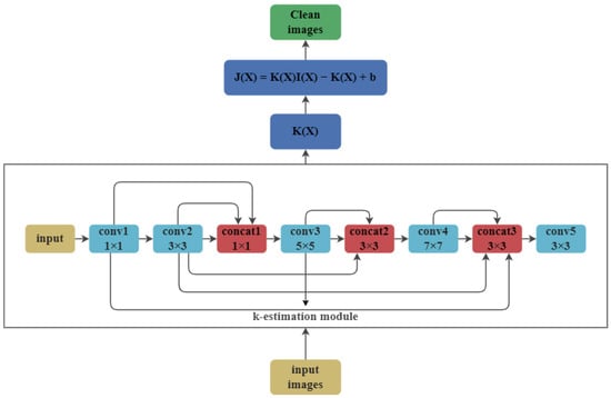
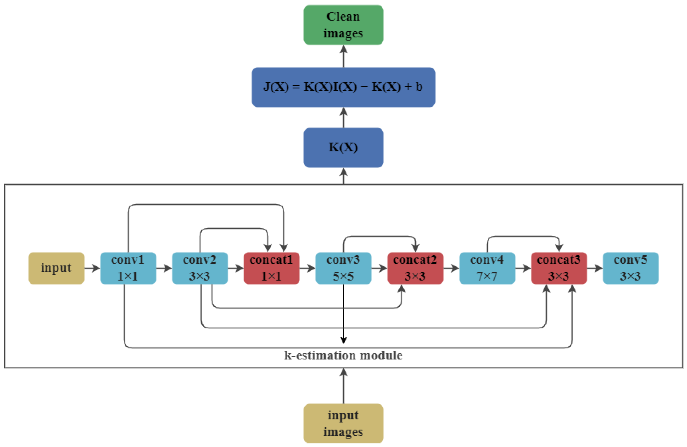
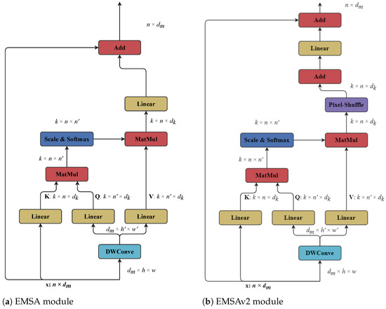
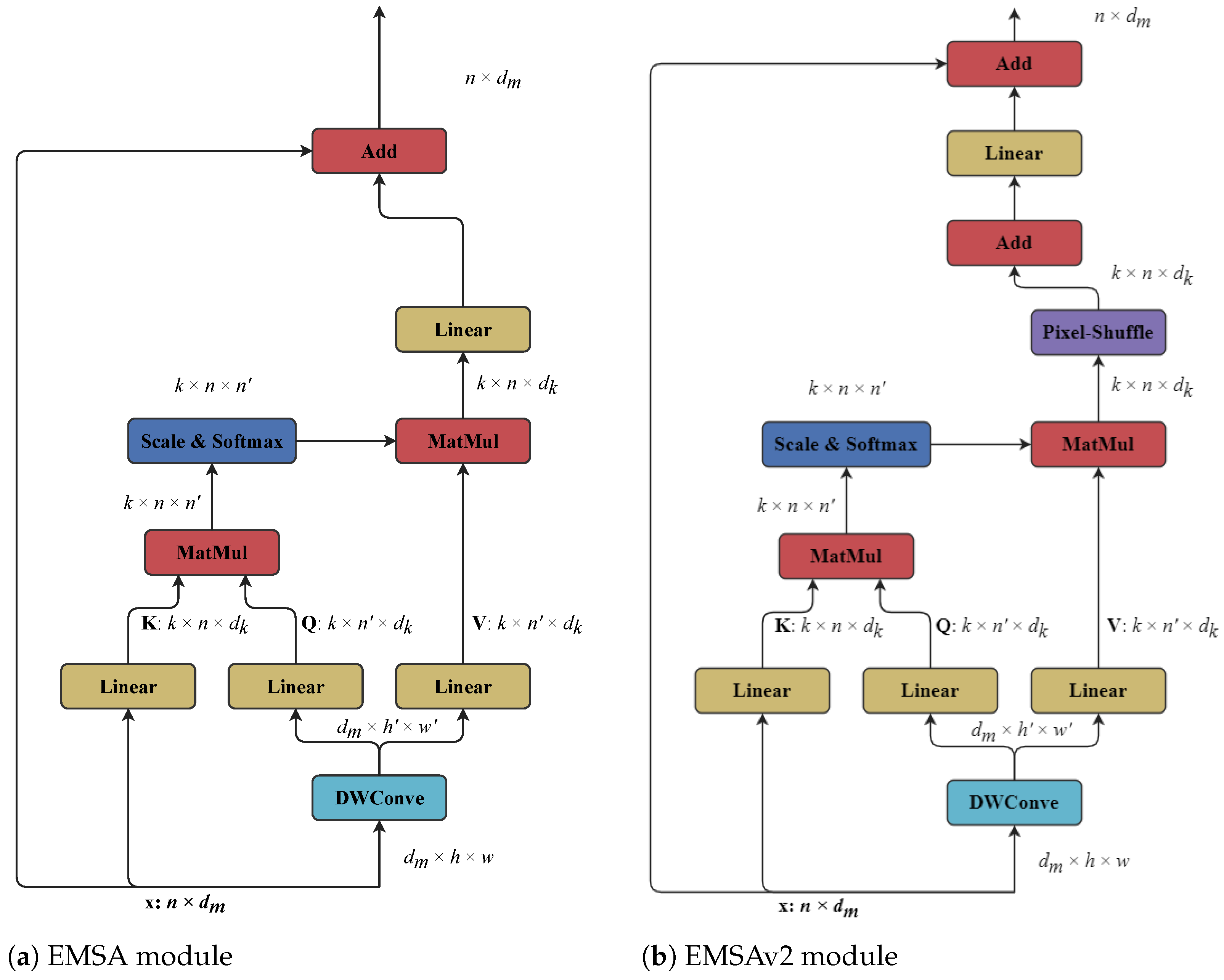
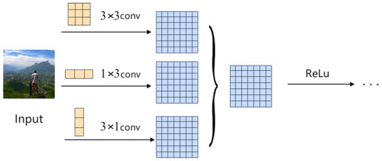
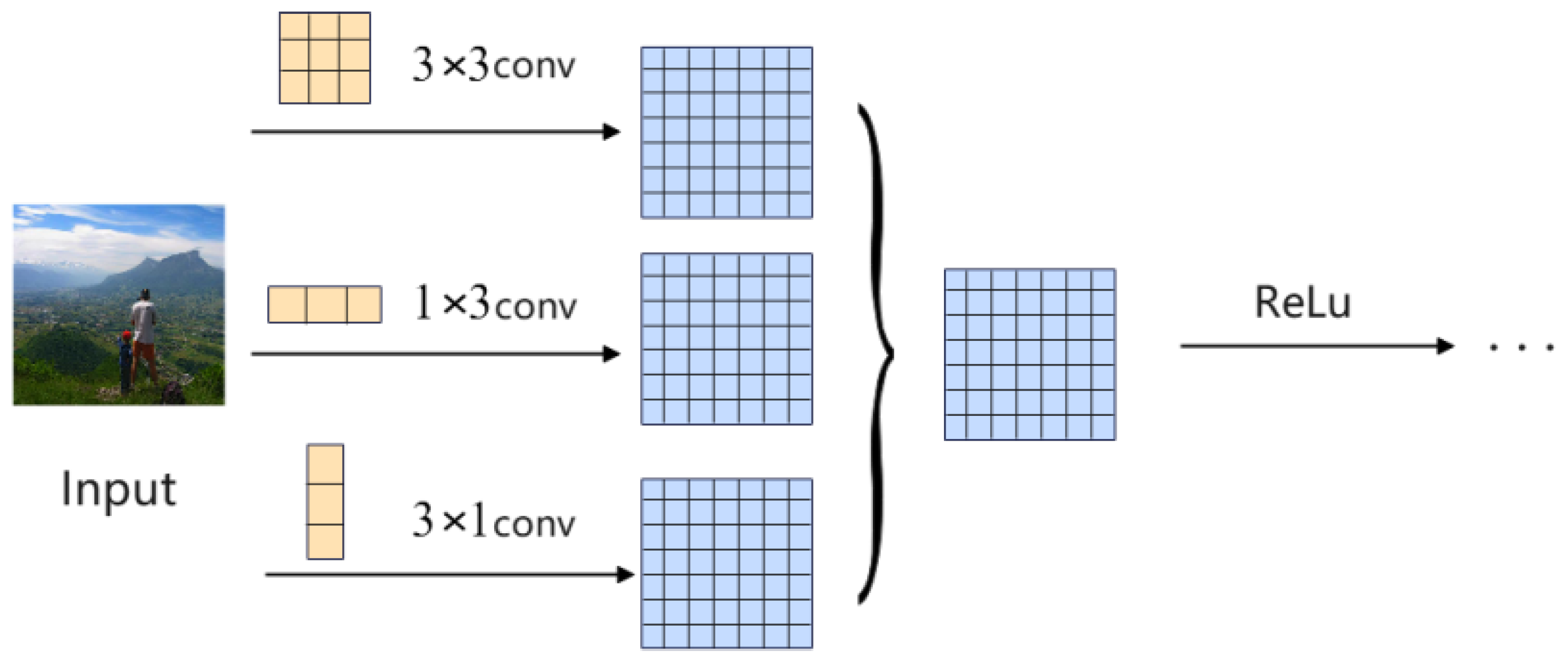
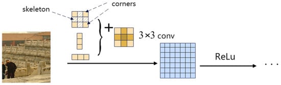
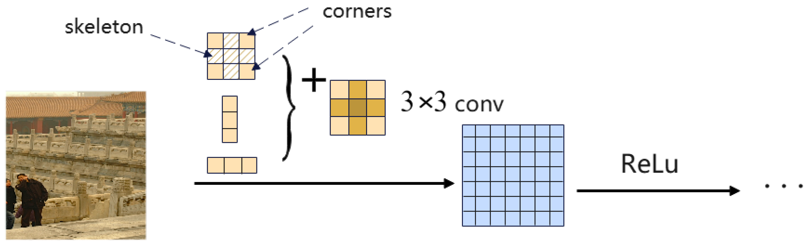
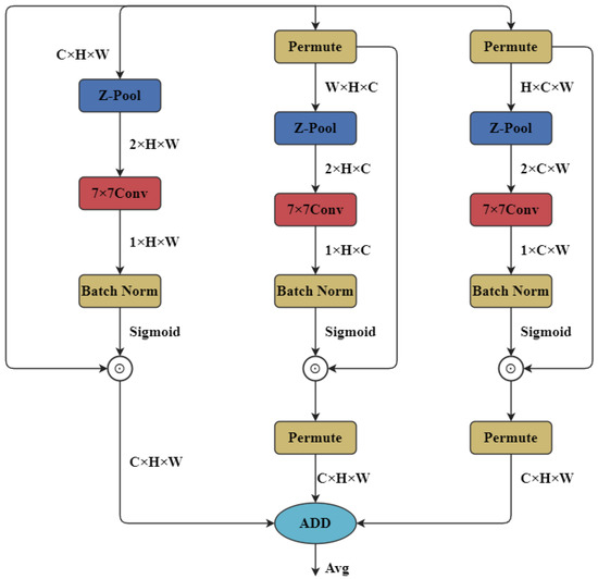


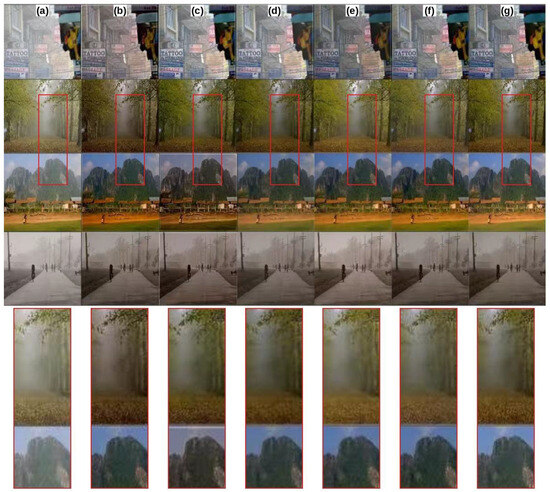
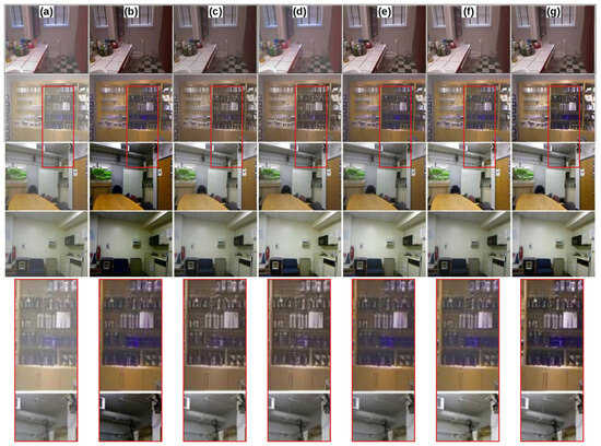
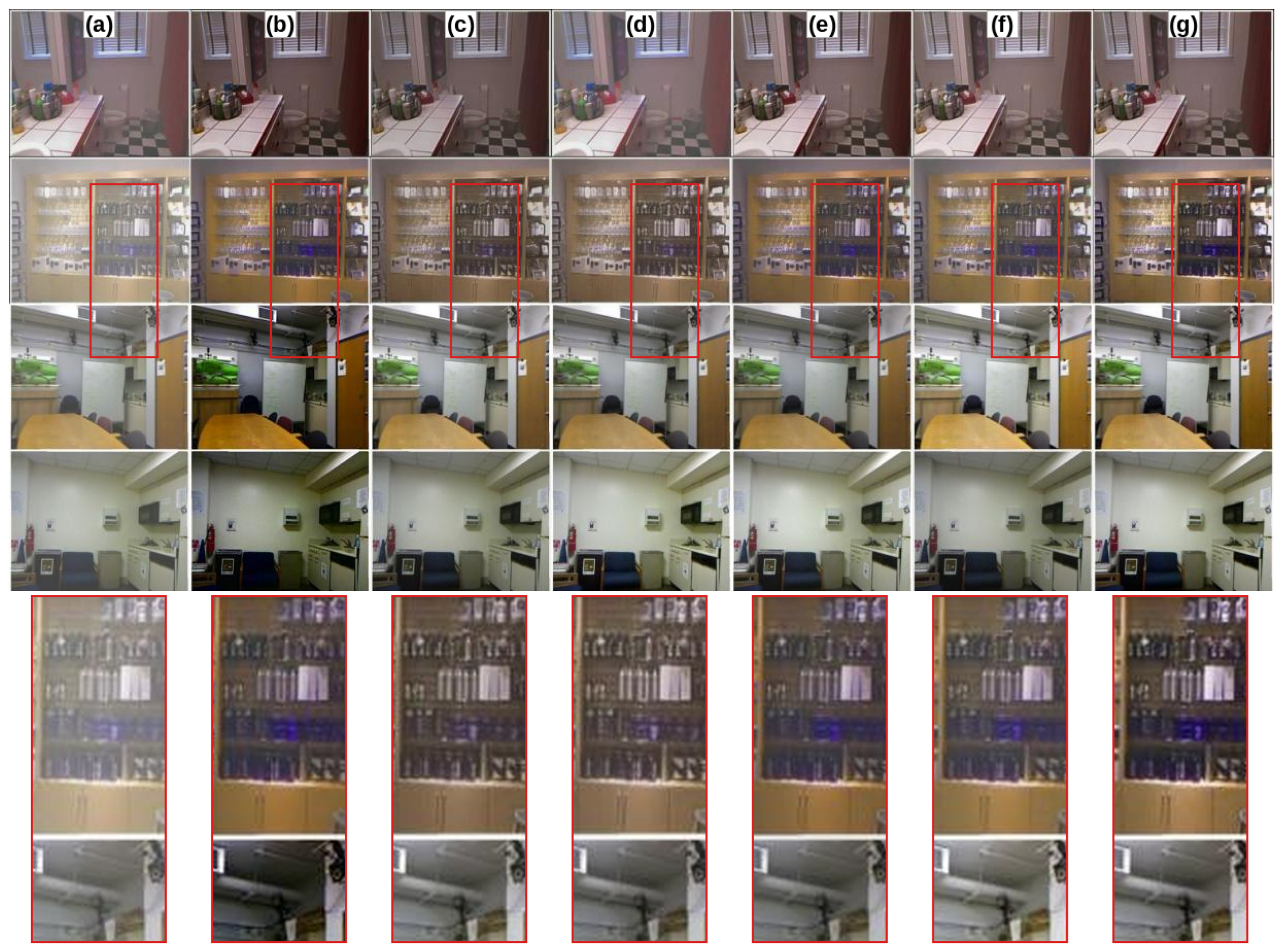
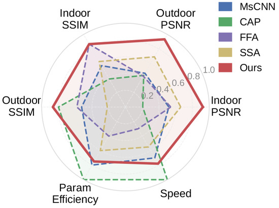
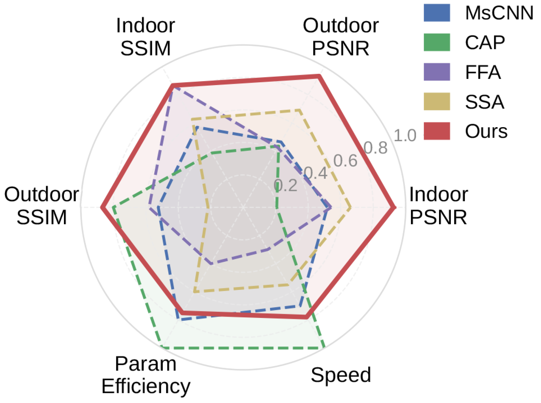
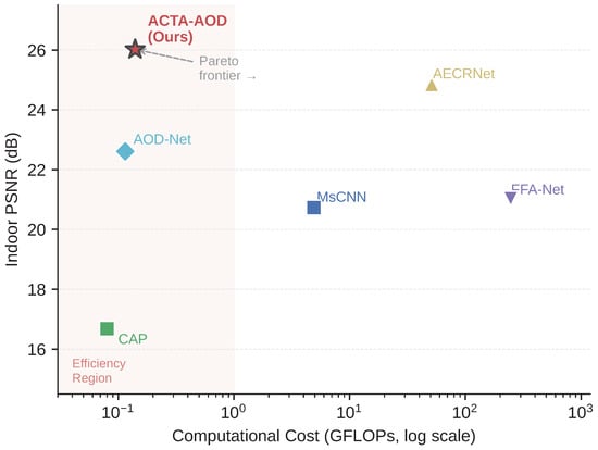
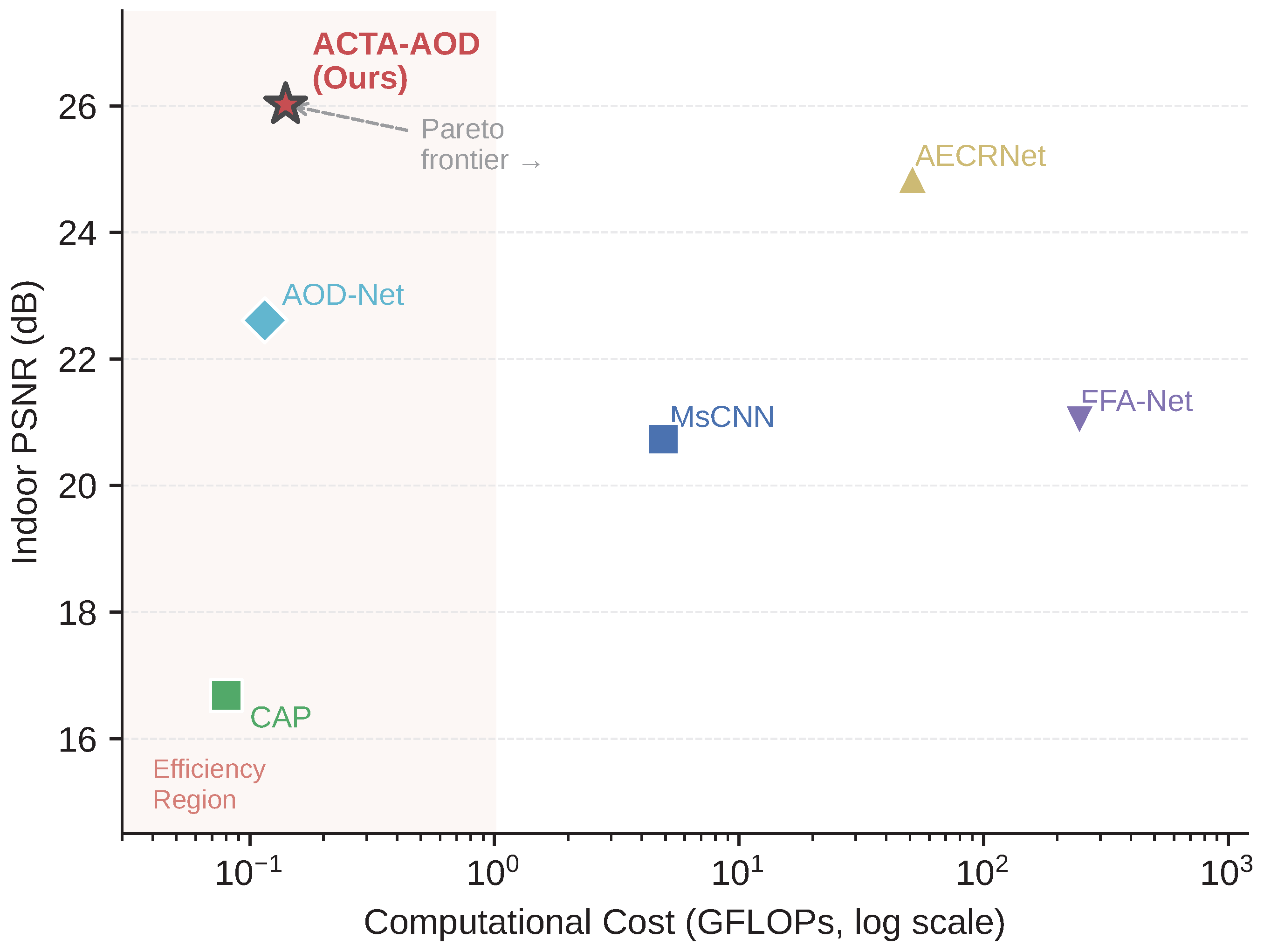
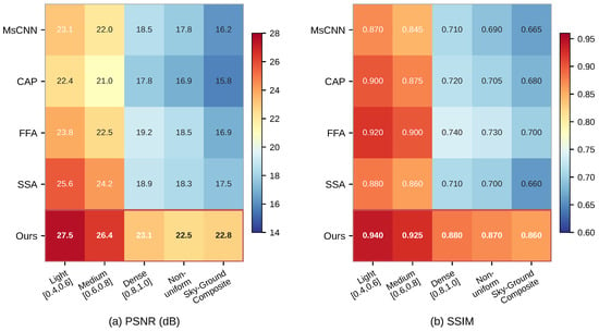
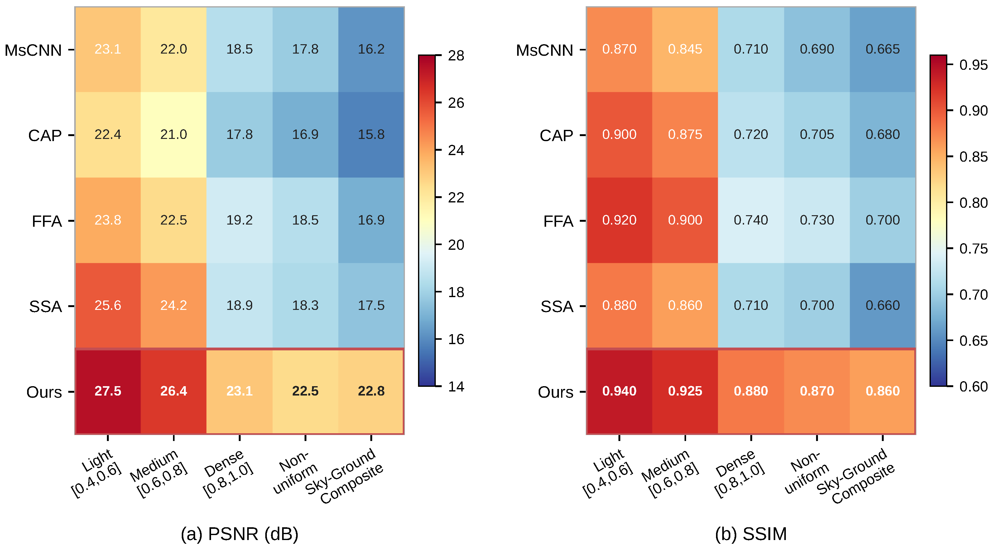
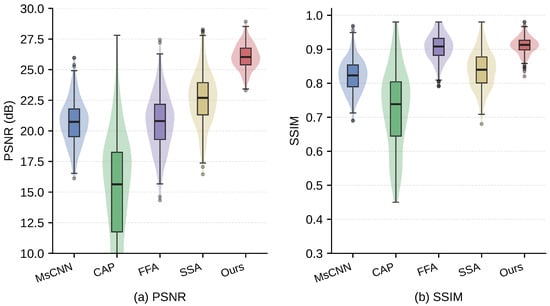
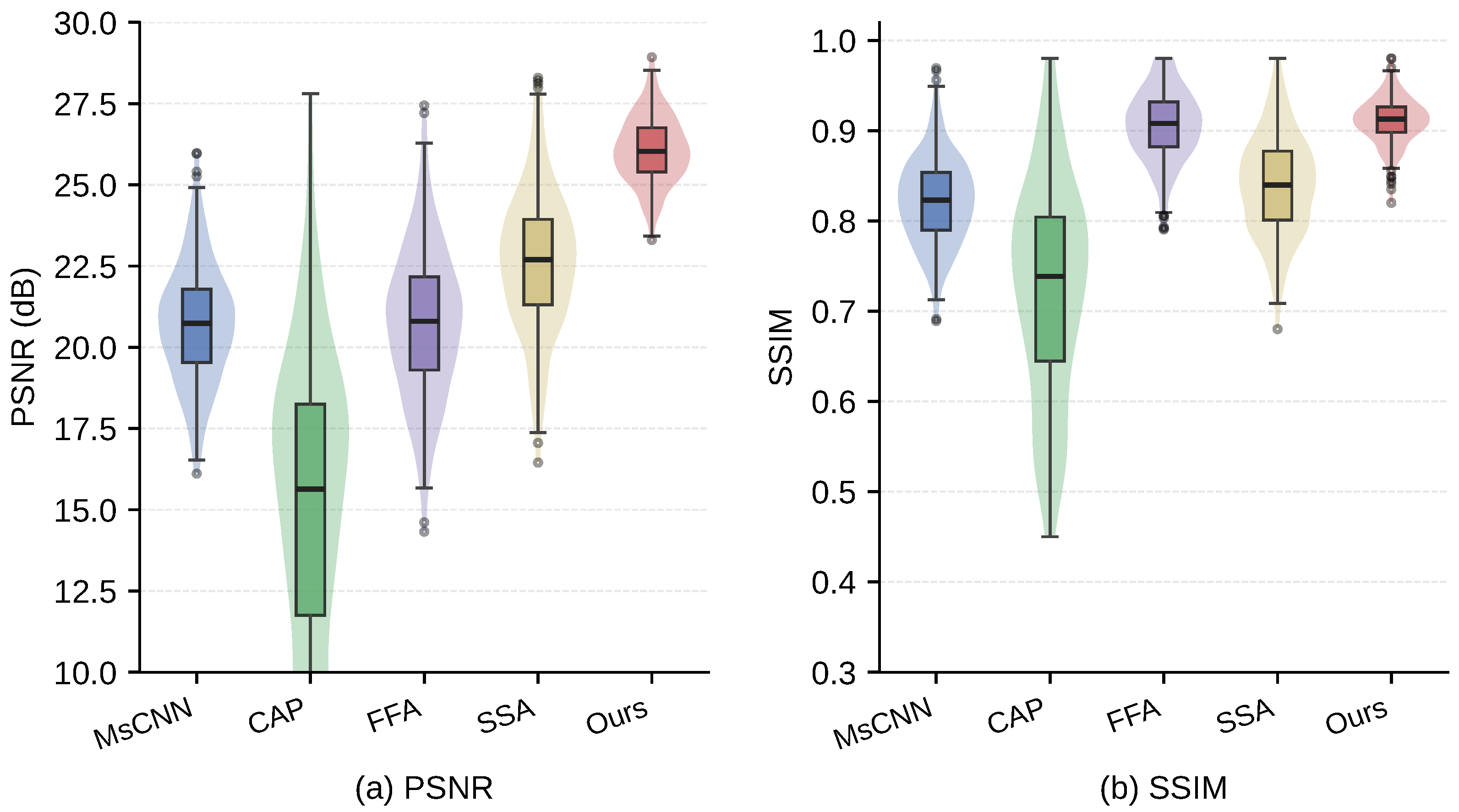
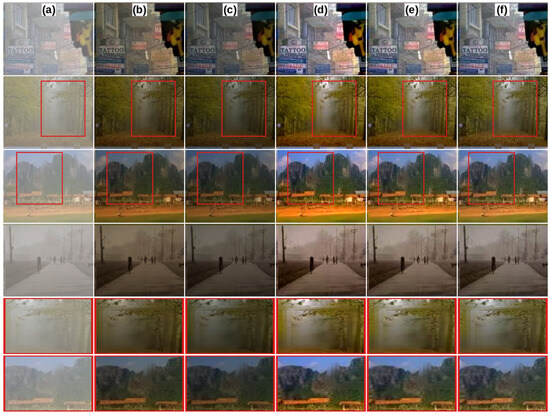
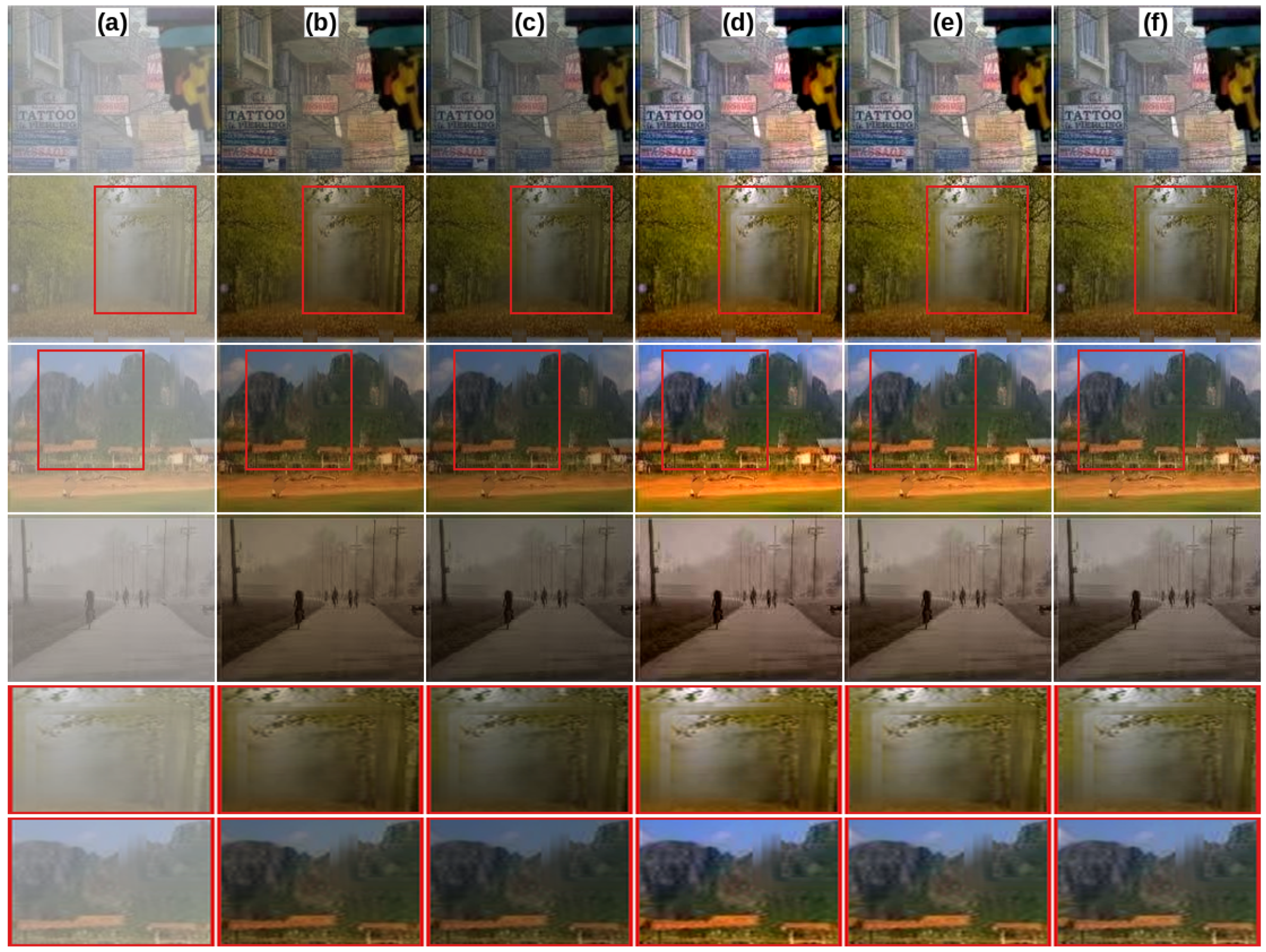
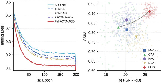
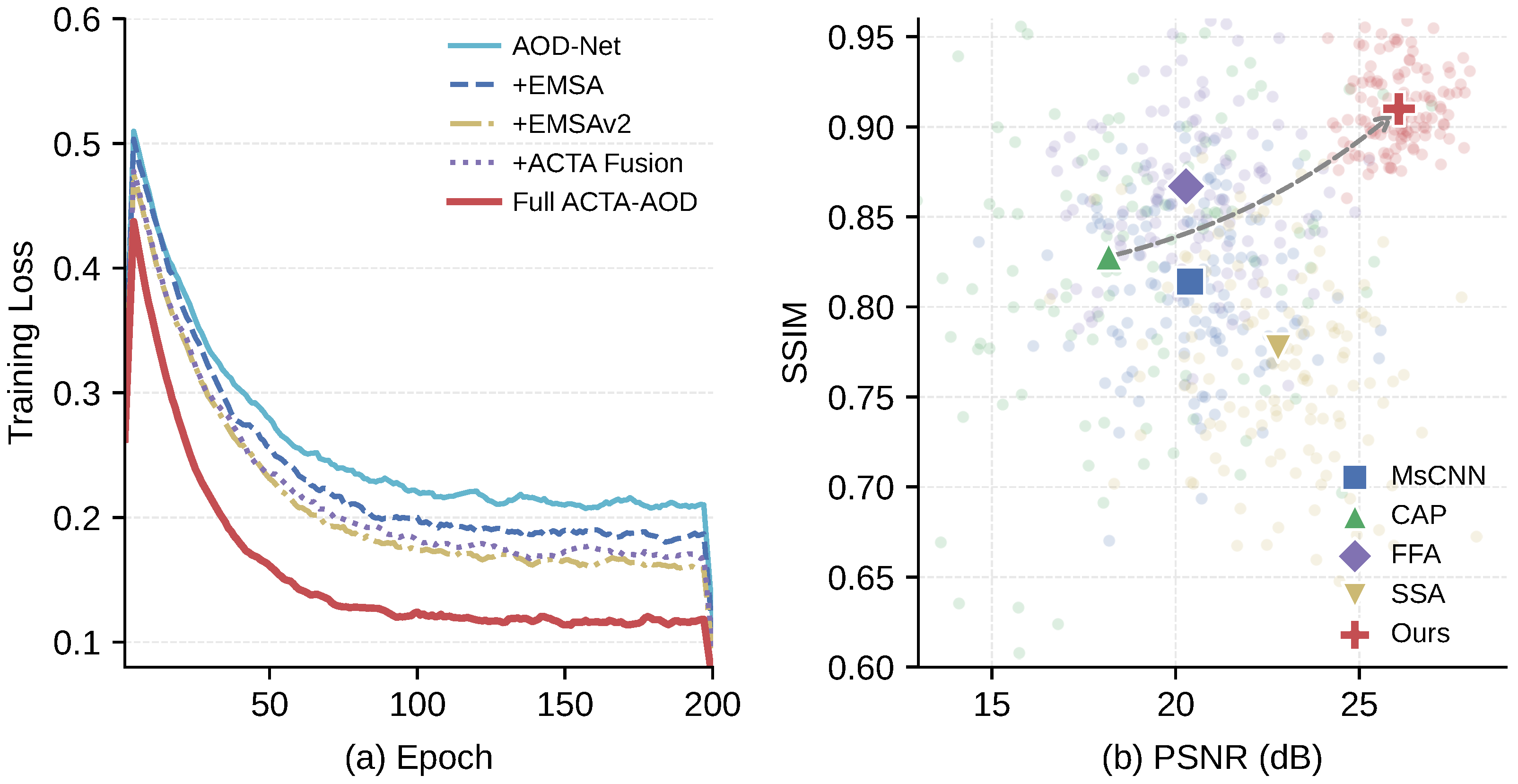
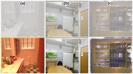
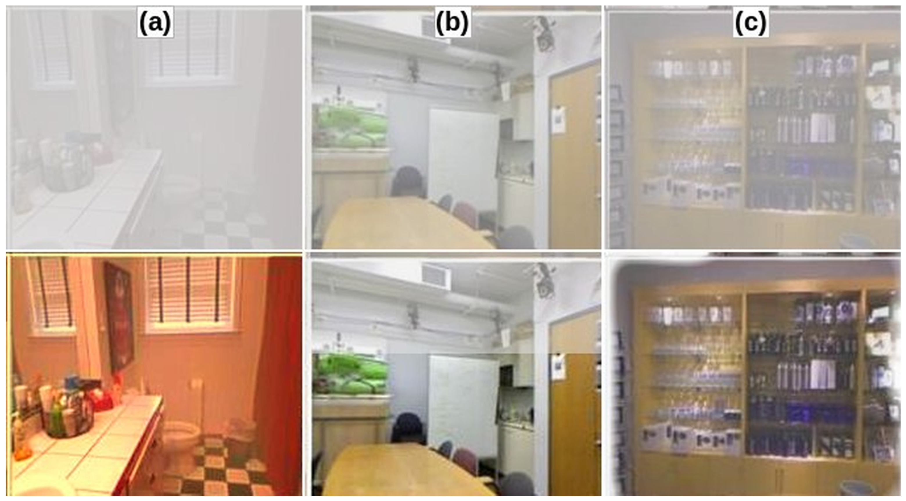

Disclaimer/Publisher’s Note: The statements, opinions and data contained in all publications are solely those of the individual author(s) and contributor(s) and not of MDPI and/or the editor(s). MDPI and/or the editor(s) disclaim responsibility for any injury to people or property resulting from any ideas, methods, instructions or products referred to in the content. |
© 2026 by the authors. Licensee MDPI, Basel, Switzerland. This article is an open access article distributed under the terms and conditions of the Creative Commons Attribution (CC BY) license.