


Abstract
Oil and gas pipelines are crucial component of the strategic infrastructure in China, but they are severely threatened by geological disasters in complex terrains. These disasters may cause pipeline rupture, leakage or explosion, resulting in significant economic losses, environmental pollution and casualties. Traditional manual disaster investigation is inefficient because the pipelines are widely distributed, access is limited and the terrain may be rugged. Therefore, efficient and accurate disaster identification and risk assessment have become a priority that the industry urgently needs to address. Taking the Jiangxi section of the West Line II Zhangshu–Xiangtan connection line as the research area, this study combines the SBAS-InSAR technology with spatial analysis based on GIS to support early disaster identification, surface deformation monitoring and vulnerability assessment. The analysis of 48 Sentinel-1A satellite images shows that the regional ground deformation range is −19.5 to 19.1 mm per year, and most areas show a slow deformation of within ±10 mm per year. The preliminary visual interpretation of the SBAS-InSAR ground deformation data yields 121 preliminary high-deformation disaster points. Combined with the 9 key assessment factors in the GIS platform and the entropy-weighted information model obtained from the geological disaster susceptibility evaluation map and using the optical remote sensing images, 21 human interference points are excluded, and finally 100 potential geological disaster hazard areas are retained. Field verification was conducted through ground reconnaissance surveys and confirmed that 78 of these areas have geological disaster hazards such as landslide, collapses, and slope water damage, providing solid technical support for geological disaster management, monitoring and early warning along the pipeline route. This study proposes a multi-source integrated framework combining SBAS-InSAR, GIS-based susceptibility assessment, and optical validation for improving the reliability of early geological hazard identification.
1. Introduction
Oil and gas pipelines are essential for oilfield development and production, serving a critical function in the transportation chain [1]. China’s oil and gas pipeline network has undergone 17 years of large-scale development. The first West–East Gas Pipeline was completed and commissioned in 2014. By the end of 2020, the total pipeline length had reached 144,000 km, ranking fourth worldwide [2]. However, oil and gas pipelines frequently cross complex geological environments and are highly vulnerable to hazards such as landslides, debris flows, ground subsidence, and earthquakes. These hazards can cause pipeline ruptures, leaks, or even explosions, leading to severe economic losses and significant environmental impacts. Moreover, the maintenance costs of the oil and gas pipelines will also change due to variations in the surrounding environment [3]. Therefore, accurately identifying geological hazards along pipeline corridors and assessing their occurrence risk have become urgent priorities for the oil and gas industry. Currently, geological hazard inspections for oil and gas pipelines rely primarily on manual patrols. Due to the extensive pipeline network and challenging terrain and road conditions along the routes, manual inspections face substantial operational and efficiency limitations. While small to medium-sized geological hazards are easily detected during routine inspections, large-scale hazards often remain unnoticed due to limited observational perspectives, yet these hazards pose substantially greater risks to pipeline infrastructure.
Therefore, incorporating geological hazard susceptibility into the management and planning of infrastructure such as oil and gas pipelines is of great importance [4,5]. By analyzing geological hazard susceptibility and considering factors such as geology, topography, and climate, the likelihood of hazards such as landslides occurring under different conditions can be evaluated [6,7]. In recent years, ground deformation monitoring technologies such as Interferometric Synthetic Aperture Radar (InSAR) have provided precise deformation measurements which penetrate cloud cover and reduce reliance on manual operations, thereby enabling effective identification of geological hazards such as landslides [8]. Integrating susceptibility assessments with time-series InSAR deformation monitoring can significantly enhance the accuracy and reliability of geological hazard susceptibility evaluations [9].
InSAR technology is a key tool in geological disaster risk management and occupies an important position in related research. Hussain et al. applied PS-InSAR combined with Sentinel-1 data to monitor ground subsidence in Peshawar, Pakistan, from 2018 to 2020, and identified a correlation between subsidence patterns and precipitation [10]. Tong et al. developed a coherence-based Small Baseline Subset (SBAS) method for the Columbia River Gorge in Washington, USA, and derived the landslide displacement time series to investigate landslide activity along the corridor [11]. In recent years, advances in remote sensing have further highlighted the unique advantages of InSAR in geological disaster monitoring and in providing early warning. Compared with traditional monitoring methods, InSAR offers higher precision, wider spatial coverage, and all-weather, continuous monitoring capabilities, thereby providing strong support for geological disaster risk management. Therefore, in this study, SBAS -InSAR ground deformation data were used to conduct a preliminary identification of potential geological disaster areas in the study region, aiming to provide a scientific basis for disaster prevention and mitigation.
In the 1980s, mathematical and statistical models based on Geographic Information Systems (GIS) developed rapidly and were widely applied, becoming important tools for assessing geological hazard susceptibility [12]. Geological hazard susceptibility evaluation can be effectively achieved through the spatial data management and analysis capabilities of GIS [13]. Early susceptibility assessment models primarily relied on experience-based qualitative methods [14]. These methods delineated disaster-prone areas using intuitive judgments of geological, topographic, and other contributory factors [15]. Subsequently, quantitative evaluation methods were gradually developed. Pradhan et al. applied a multivariate logistic regression model incorporating factors such as rock type, slope, and land use to assess landslide susceptibility in the Penang, Kimanur, and Selangor regions of Malaysia [16]. They further performed cross-validation, which demonstrated relatively high model accuracy. The information quantity model is a quantitative evaluation method grounded in information theory. It quantifies each evaluation factor by analyzing its relationship with the occurrence of geological hazards and calculating the corresponding information content. This model objectively reflects the influence of different factors on geological hazard susceptibility. By integrating multiple factors, it enables a comprehensive evaluation of geological hazard susceptibility within the study area. In this study, the selection of evaluation factors fully accounts for the geological, topographic, and hydrological conditions along the oil and gas pipeline. Therefore, based on the GIS platform, this study selected nine evaluation factors and applied the information quantity model to construct a susceptibility assessment system for geological hazards along the oil and gas pipeline.
However, because the pipeline corridor traverses areas with intensive human activities, such as residential zones and farmlands, the ground deformation detected by SBAS-InSAR is not solely attributable to geological hazards. To address this issue, multi-temporal optical remote sensing imagery was utilized for auxiliary screening. It is important to clarify that in densely vegetated areas, optical imagery cannot directly reveal ground deformation beneath the canopy. Nevertheless, it excels at detecting changes in land cover and surface features. By visually comparing optical images from different dates, we can efficiently identify surface modifications indicative of non-hazard anthropogenic activities—such as building construction, cultivated land reclamation, or forest clearing. Excluding these human-induced deformation areas from the preliminary InSAR-based inventory improves the accuracy of early geological hazard identification along the pipeline. Consequently, this study re-evaluates the preliminary geological hazard zones identified from SBAS-InSAR deformation data, compares them with susceptibility assessment results, and refines the screening process to improve the accuracy of hazard detection.
Although previous studies have demonstrated the effectiveness of InSAR and GIS-based susceptibility assessment in geological hazard identification, many of them rely on single-source data or loosely integrated frameworks, limiting their ability to fully exploit complementary information from multi-source datasets [17]. InSAR alone cannot fully capture geological conditions and may lack interpretability without auxiliary data [18]. Recent hybrid approaches have attempted to integrate multi-source data; however, they often lack systematic validation using independent datasets such as optical imagery or field surveys. Moreover, few studies explicitly address the differentiation between deformation caused by geological hazards and that induced by human activities, which may lead to false positives. Therefore, there remains a research gap in developing an integrated, multi-source verification framework that combines deformation monitoring, susceptibility assessment, and validation mechanisms to improve the reliability of early hazard identification.
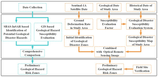
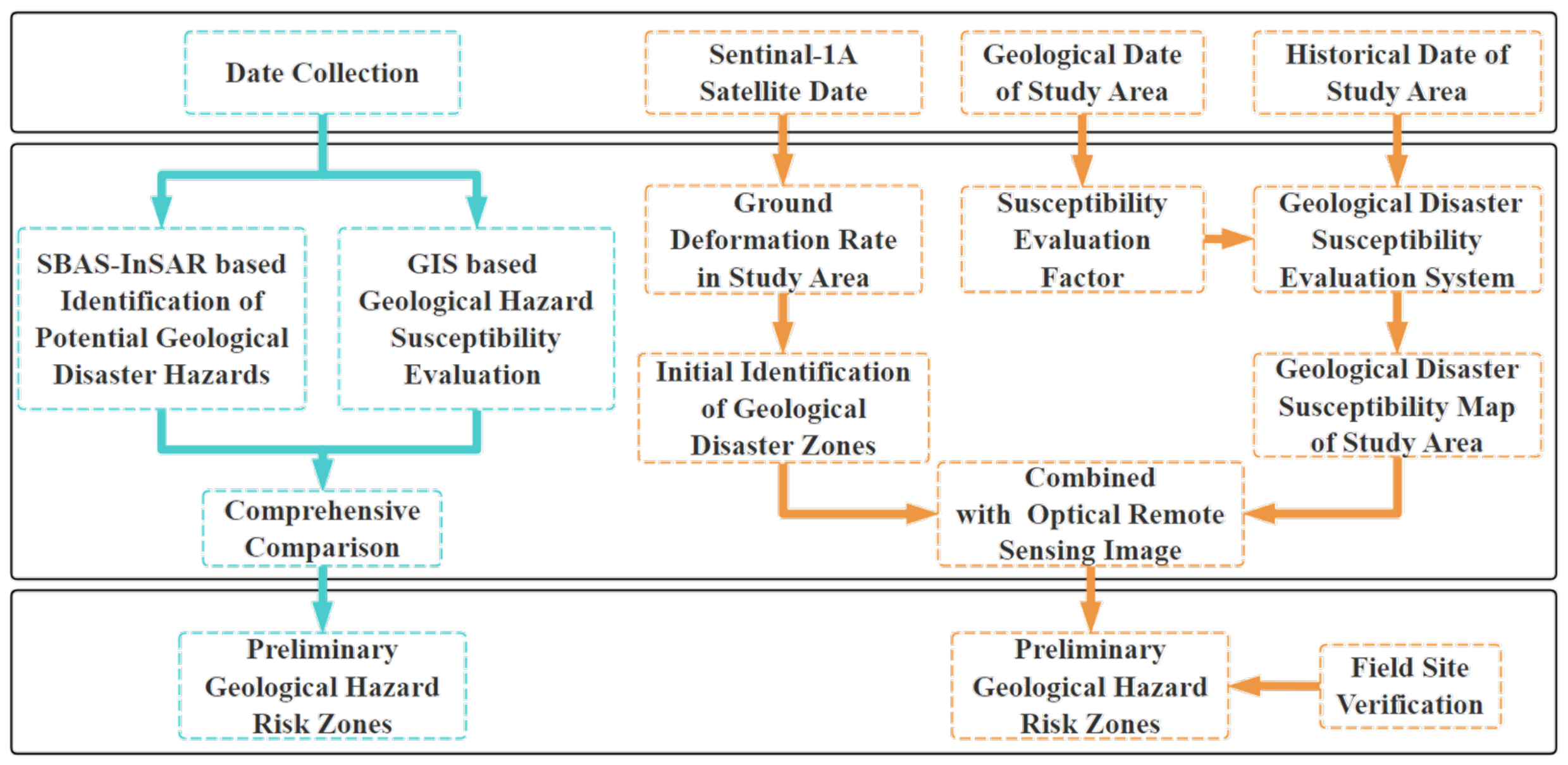
This study focuses on the Xiangtan Connection Line of the West–East Gas Pipeline and employs SBAS-InSAR technology to identify early-stage geological hazard points. Based on these results, geological data were collected, a susceptibility evaluation model was developed, and GIS-based assessments of geological hazards along the pipeline were performed. The research components include: (1) applying SBAS-InSAR multi-temporal analysis to derive surface deformation rates and generate deformation distribution maps, followed by preliminary visual interpretation of geological hazards to identify early warning points; (2) processing the data in GIS to select key factors such as lithology, slope, and normalized vegetation index, analyzing their correlations with geological hazards, classifying these factors, and assigning appropriate weights to construct a susceptibility evaluation model using the information quantity method. Historical disaster data and the entropy weighting method were used to determine factor weights, and a geological hazard susceptibility map was generated to assess regional risk levels; and (3) integrating optical remote sensing imagery with SBAS-InSAR–derived preliminary hazard areas and overlaying them with GIS-based susceptibility results for comparative analysis. Misidentified points resulting from human activities were removed to obtain the locations of the final early-stage geological hazard areas along the pipeline. Field verification was conducted to validate the results and provide practical guidance for pipeline disaster risk management. The overall research workflow is shown in Figure 1.
Figure 1.
Research workflow.
2. Methods and Data
2.1. Study Area
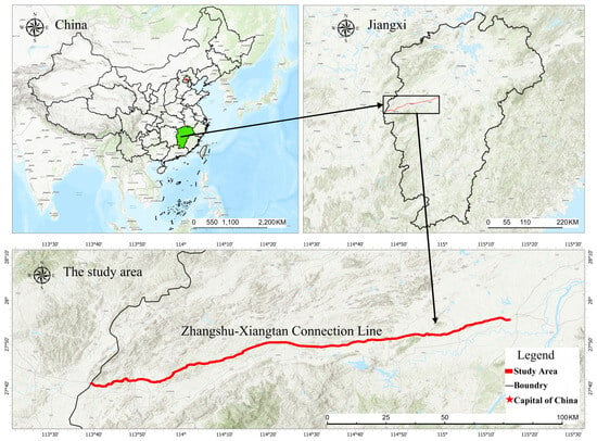
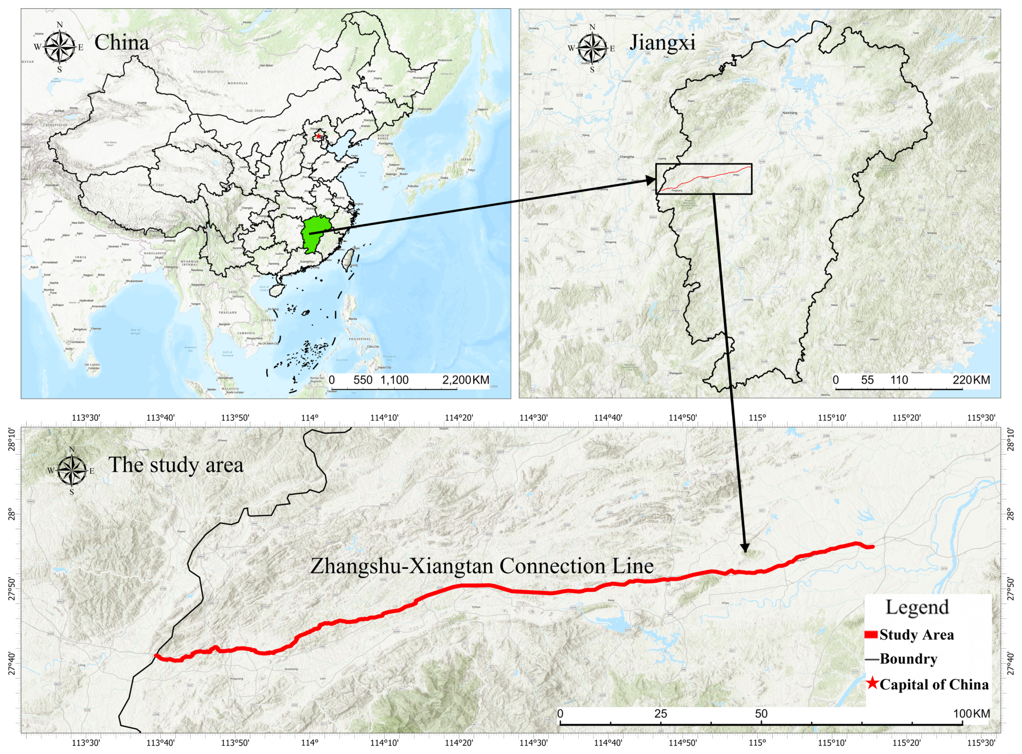
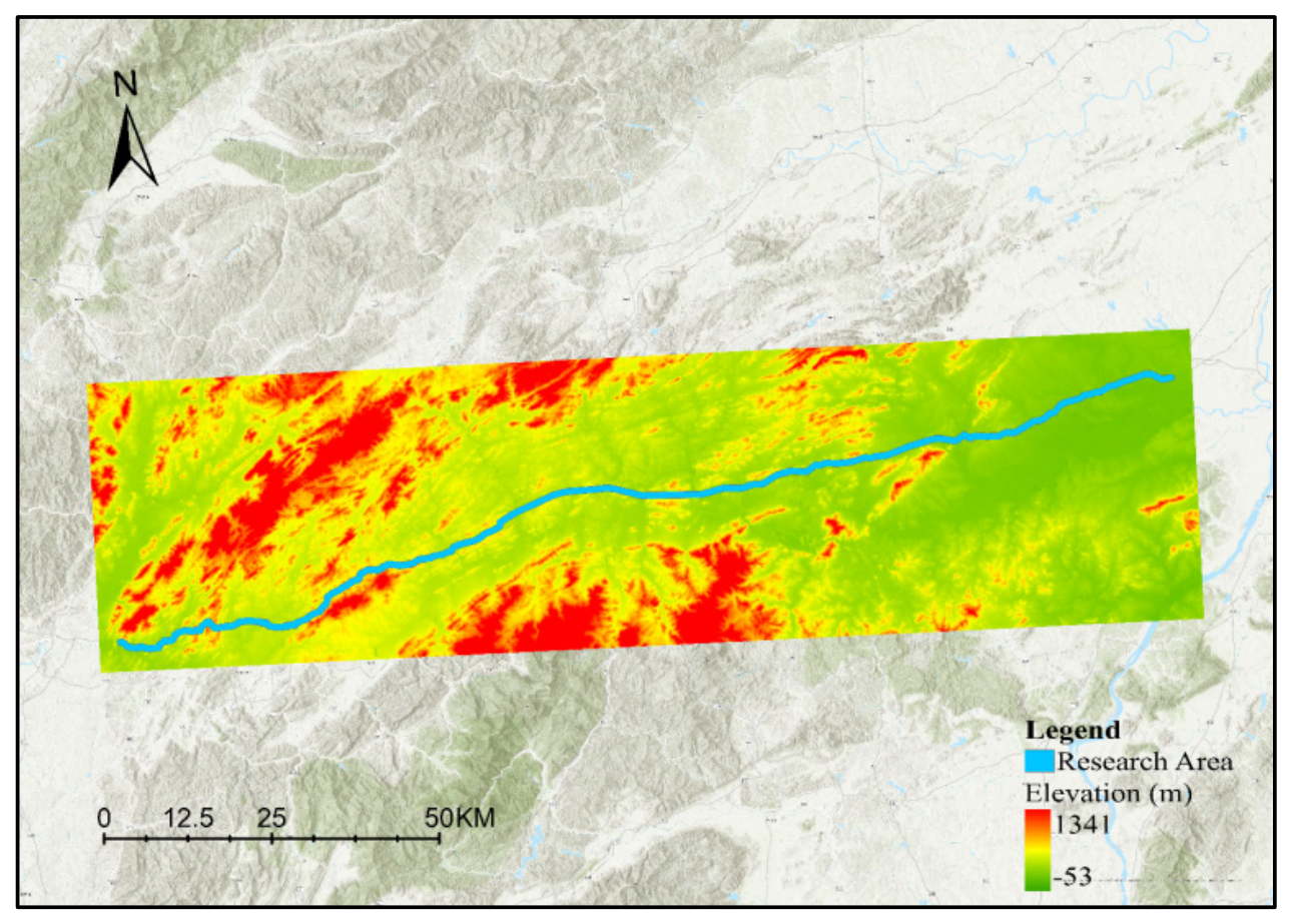
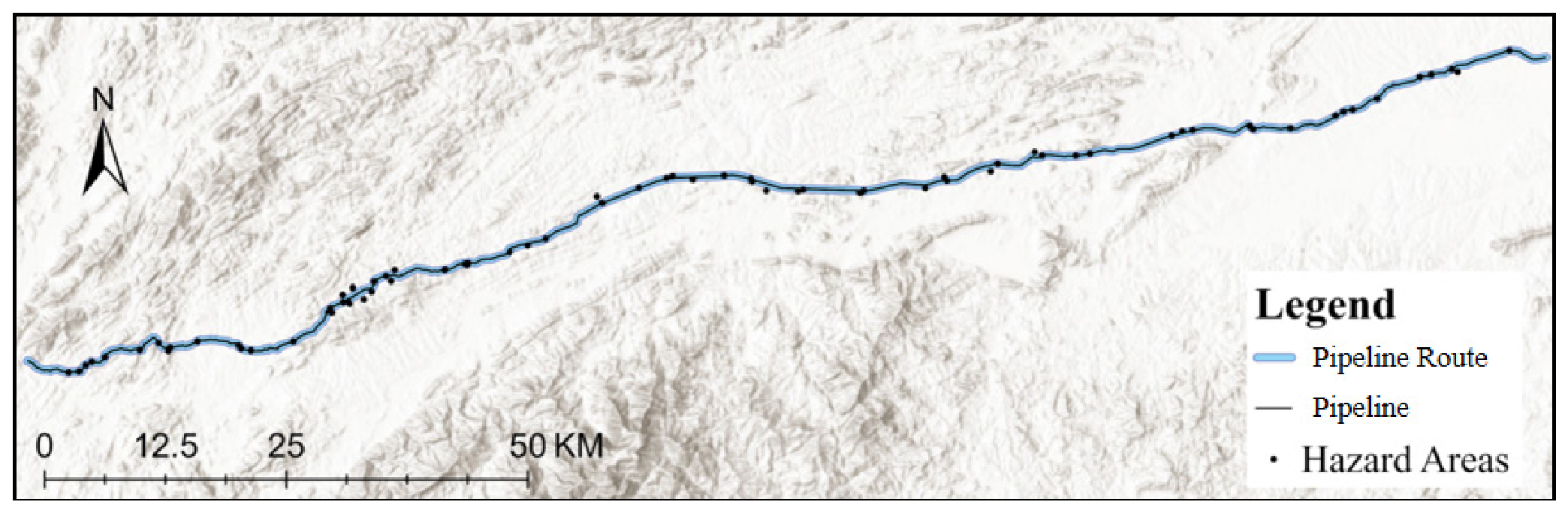
The Xiangtan Connection Line refers to the Jiangxi section of the West Line II Zhangshu–Xiangtan Connection Line (Figure 2). Oriented east–west, the pipeline begins at Zhangshu Distribution Station, passes through Xinyu City, Fenyi County, Yichun City, and Shangli County, and ends at the border of Jinshui City, Pingxiang City, and Liling City in Hunan Province. The pipeline extends 178.91 km in length and includes three stations and seven valve chambers along its route. The study area is defined as a 500 m buffer zone around the pipeline, according to relevant standards.
Figure 2.
Location of the study area.
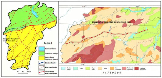
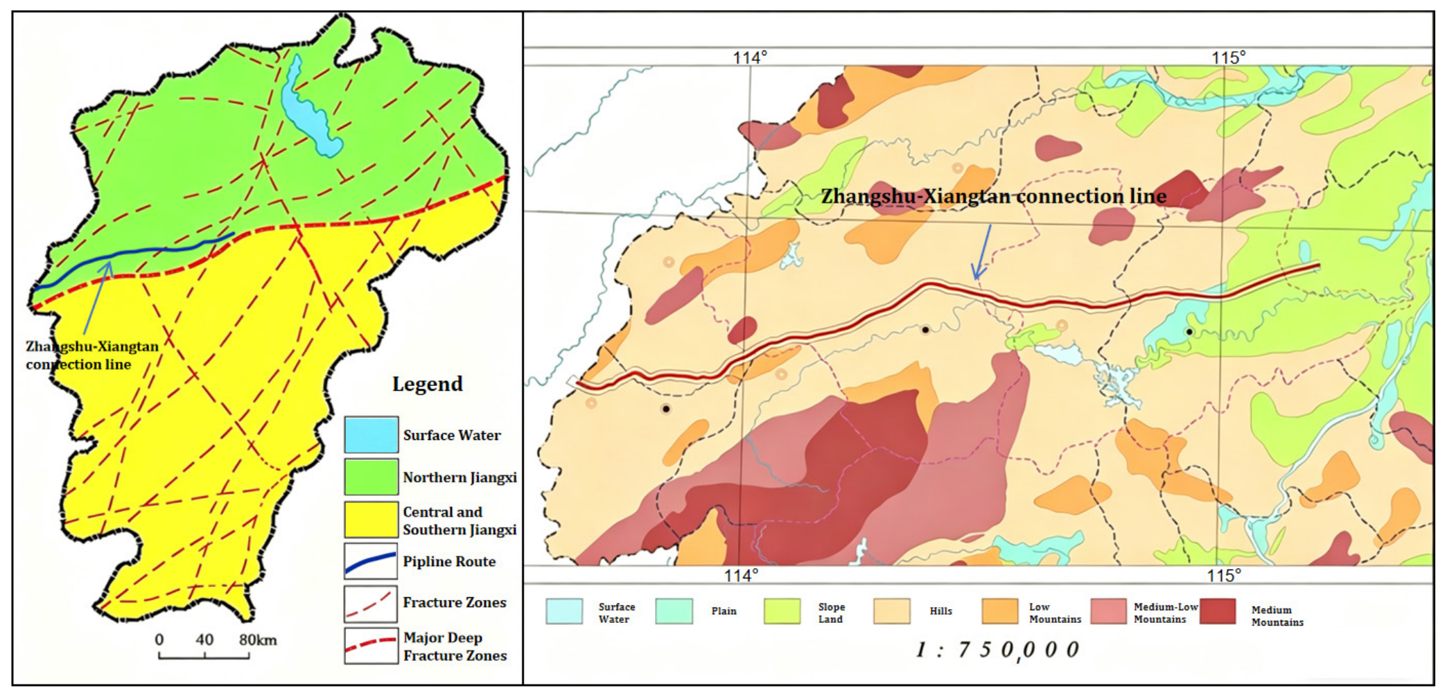
The study area is located in Jiangxi Province, within the subtropical monsoon climate zone, which is characterized by distinct seasons and abundant rainfall. The region has an annual average temperature of 17–20 °C, with extremes ranging from −12.8 °C to 43.3 °C. Annual precipitation ranges from 1341 to 1934 mm, with higher frequency and intensity in mountainous areas than in basins. Geographically, Jiangxi is part of the Jiangnan hilly region, bordered by mountains to the east, west, and south. The central region features alternating hills and river valley plains, whereas the northern section consists of the Poyang Lake Plain, with terrain generally sloping northward. The Western Second Line connecting Zhangshu and Xiangtan (Jiangxi section) crosses the following geological zones from west to east: tectonic erosion lowland, tectonic erosion hilly area, erosional low ridge area, tectonic erosion hilly area, erosional low ridge area, alluvial valley plain, and erosional low ridge area. A schematic geological map along the pipeline route is presented in Figure 3. The pipeline route traverses alternating plains, hills, and low mountains, with multiple intersections of major fracture zones. These terrain transitions and structurally weakened belts correspond to the primary geohazard-prone sections identified in this study.
Figure 3.
Geomorphological zonation and regional fault distribution along the Zhangshu–Xiangtan pipeline.
In the context of pipeline integrity management, the combination of abundant monsoon rainfall and the alternating soft/hard rock lithology renders the right-of-way susceptible to specific types of shallow geological hazards. Rather than deep-seated tectonic deformation, the primary threats identified in this corridor are shallow landslides and unstable slopes triggered by rainfall infiltration, and fluvial erosion at river crossings or floodplains. These hazards pose a direct risk to the pipeline by reducing burial depth, exposing the steel casing, or inducing lateral soil movement that leads to excessive bending stress. Consequently, this study focuses on the early identification of surface deformation anomalies indicative of these specific mass-wasting and erosion processes.
2.2. SBAS-InSAR-Based Geological Hazard Identification
SBAS-InSAR technology is based on the short baseline subset (SBAS) principle. When processing multiple primary images, one image is designated as the common reference to guide subsequent image registration. After generating multiple interferometric subsets, DEM data is used to model and remove terrain phase components for each interferometric pair, producing time-series differential interferograms. Upon phase unwrapping, precise phase data for each coherent target—including deformation, atmospheric delay, and orbital error phases—is obtained. These error components can be effectively corrected using time-series filtering or polynomial fitting. Notably, using multiple primary images in SBAS-InSAR may result in rank deficiency during the joint solution of interferometric subsets. To address this issue, the method applies singular value decomposition (SVD) combined with least-squares minimization under minimum-norm constraints, allowing for the accurate inversion of surface deformation over time and for an extraction of the mean deformation rate across the entire time series [19]. The working principle is summarized as follows:
Given N SAR images of the target area, labeled t1, …, ti, …, tN in chronological order, the images are partitioned into X short baseline sets by applying temporal and spatial baseline thresholds. Differential interferometry is then applied to the images within each set to generate M differential interferograms, where M satisfies:
Assuming all phase signals have been unwrapped and calibrated to a deformation-stable reference point, with t1 denoting the initial time, the differential interferometric phase difference at ti (i = 2, …, N) relative to t1 is φ(ti), and the processed differential interferometric phase difference is δφ(t_k) (k = 1, …, M). The resulting time series is then expressed as:
The interferometric phase of any pixel (x, y) in the k-th interferogram (k = 1, …, M), neglecting atmospheric and topographic effects, is expressed as:
Here, λ denotes the radar wavelength, while t_A and t_B represent the acquisition times of the primary and secondary images for the k-th differential interferogram, respectively. The displacement fields d(t_A, x, y) and d(t_B, x, y) correspond to the cumulative deformation along the line-of-sight direction relative to the primary images at t_A and t_B, respectively. The formula for φ(t_A, x, y) is given as follows:
Let denote the primary and secondary image sequences corresponding to M differential interferograms in chronological order, respectively, where
The following expressions for the observed differential interferometric phase can then be established:
As shown, Equation (6) represents a system of N equations with M unknowns, which can be expressed in matrix form as:
In this formula, A denotes an M × N approximate correlation matrix, where each row corresponds to the differential interferometric phase of a single scene, and each column represents a SAR image. The symbol φ denotes the phase value of each SAR image, while δφ denotes the phase value of each differential interferometric image.
By converting the solution of the differential phase in Equation (7) into the solution for the average phase rate v, we obtain:
Equation (7) then can be transformed into:
In this equation, B denotes an M × N coefficient matrix. When B is of full rank, the deformation rate can be estimated using the least-squares method. However, as previously mentioned, N-perspective SAR images are typically divided into X short baseline sets, reducing the rank of matrix B to N − X. Since the rank is no longer full, B becomes a singular matrix. This system then has infinitely many solutions, necessitating the use of the singular value decomposition (SVD) method. Finally, once the average phase rate is obtained, the corresponding deformation can be calculated according to the temporal interval of the images.
This study utilized Sentinel-1A satellite data from the European Space Agency (ESA), launched on 3 April 2014, for SBAS-InSAR processing. Sentinel-1, equipped with a C-band SAR sensor, is an Earth observation satellite launched by the European Space Agency’s Copernicus Program in 2014 [20]. The satellite collects deformation data by transmitting microwave signals from its SAR sensor to surface objects and receiving the reflected signals [21]. Detailed satellite parameters are listed in Table 1. A total of 48 Synthetic Aperture Radar (SAR) images from Sentinel-1A, acquired between 9 January 2021, and 7 December 2024, were obtained, with the data listed in Table 2.
Table 1.
Basic parameters of Sentinel-1A satellite data.
Table 2.
List of Sentinel-1A satellite date.
In the InSAR data processing workflow, orbital information was used to obtain accurate satellite position and velocity data [22]. Any deviation in orbital data can induce baseline errors, which appear as visible residual fringes in interferograms, thereby compromising data accuracy and reliability. Therefore, incorporating high-precision satellite orbit data for InSAR correction is essential. The required orbital data were obtained from NASA EARTHDATA.
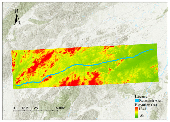
A Digital Elevation Model (DEM) provides a digital representation of a region’s topographic elevation, playing a critical role in InSAR data processing and subsequent geological hazard assessments. For this study, DEM data for the research area were obtained from the official website of the Geospatial Data Cloud (https://www.gscloud.cn/search (assessed on 5 May 2025)). A DEM dataset with 30 m spatial resolution was selected for this study, as shown in Figure 4.
Figure 4.
DEM data in study area.
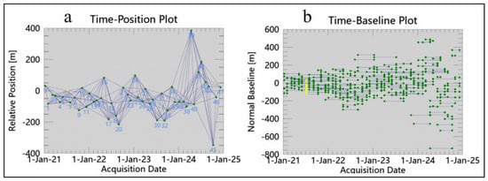
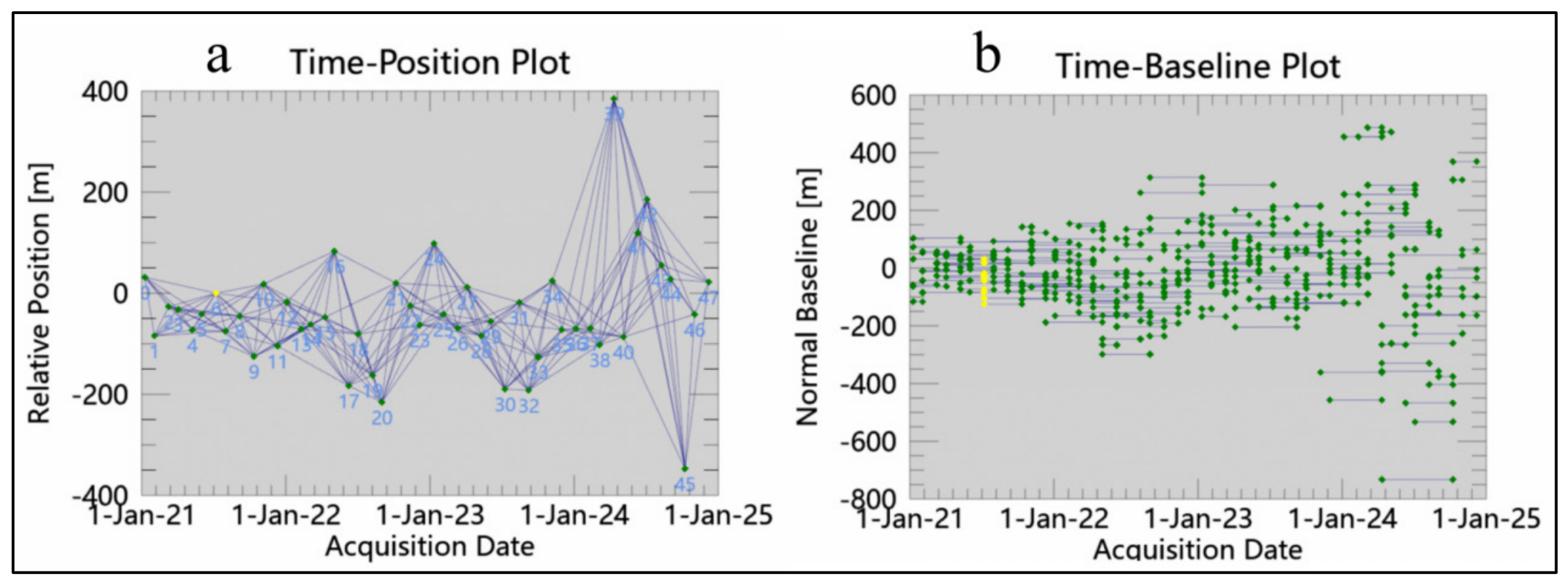
Figure 5a shows the acquired spatiotemporal baseline map, and Figure 5b shows the relative temporal baseline map. Yellow dots indicate the supermaster image, whereas green dots represent the secondary images. The workflow begins with interferometry operations, including interferogram generation and flattening, adaptive filtering, coherence generation, and phase unwrapping. This is followed by the registration of all interferograms to the supermaster image. Ground control points (GCPs) are subsequently used for refinement and re-georegistration. Two inversion stages are subsequently performed: the first estimates displacement rates and residual terrain while optimizing the data, and the second calculates time-series displacements with atmospheric filtering to remove interference. Finally, geospatial data are projected onto the WGS-84 coordinate system to complete the geocoding. After completing all the above steps, the ground deformation data of the research area can be obtained. Subsequently, the ground velocity variation rate is classified according to relevant standards and research experience into different grades. Combined with visual interpretation, a preliminary identification is made, and the initial geological hazard areas are obtained.
Figure 5.
(a) Spatiotemporal baseline. (b) Relative time baseline.
2.3. GIS-Based Disaster Susceptibility Assessment
This study employs the information quantity method, which has a simple structure, strong adaptability, and broad applicability, fully satisfying the research requirements. All GIS-based spatial analyses and map generations were performed using ArcGIS Pro 3.5. The information quantity method evaluates geological disaster susceptibility by analyzing entropy values associated with disaster occurrences. Based on the formation conditions and triggering factors of geological disasters an assessment model is established on a GIS platform to determine the correlations between geological hazards and their contributing factors. By calculating the information quantity values of the triggering factors, the correlations between influencing factors and geological disasters can be quantified. Ultimately, the susceptibility assessment results are derived and represented by the total information quantity value. A higher information quantity value indicates a greater likelihood of geological disasters occurring [23].
This study initially identified nine evaluation factors, including elevation, slope, topographic relief, land use type, fault density, topographic humidity index, slope curvature, vegetation normalized index, and lithology, based on research experience and collected data. The selection of these factors is based on a comprehensive review of previous studies, data availability, and their capability to represent key controlling conditions such as topography, geology, hydrology, and human activities [24].
Specifically, slope, slope curvature, and topographic relief reflect terrain conditions; lithology and fault density represent geological structure; NDVI and land use indicate surface cover and human activity; while TWI captures hydrological conditions. These factors collectively ensure a comprehensive representation of the mechanisms driving geological hazard occurrence. Although some correlation may exist among factors such as slope, curvature, and relief, the entropy weight method reduces the influence of redundancy by assigning weights based on information contribution. Therefore, the impact of multicollinearity is considered limited.
The impact weights of each factor on geological disasters were first determined. Based on analysis and literature references, graded values were assigned to these factors. The weighted sum of the assigned values was then calculated, and the final susceptibility assessment map was generated using the natural breaks classification method.
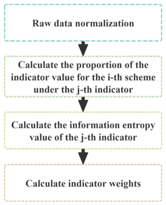
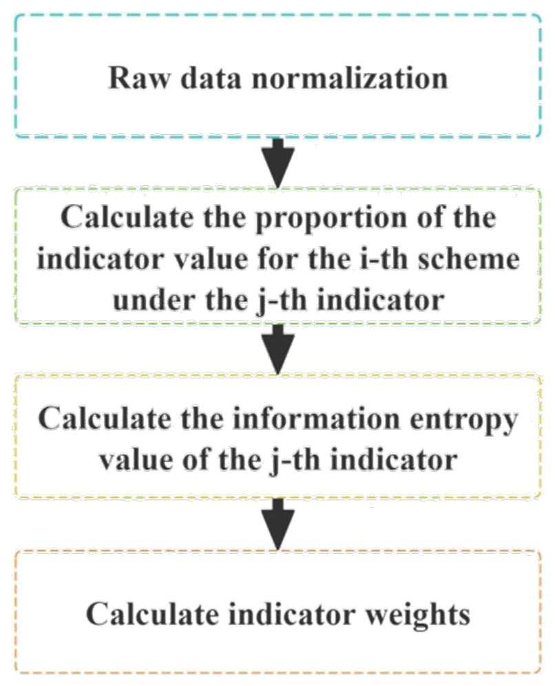
The entropy weighting method [25] is employed to assign weights to the evaluation indicators of geological disasters. The entropy weight method was selected because it determines weights objectively based on data variability, avoiding subjective bias associated with expert-based methods such as AHP. Compared with machine learning methods, it requires less training data and is more suitable for studies with limited samples. The basic calculation steps are illustrated in Figure 6.
Figure 6.
Entropy weighting method flow chart.
The purpose of data normalization is to standardize the measurement units of all indicators. For positive indicators, the normalization formula is given as follows:
For negative indicators, the calculation formula is given as follows:
Positive indicators refer to factors for which higher values correspond to a greater probability of geological disasters, whereas negative indicators denote factors for which higher values correspond to a lower probability of geological disasters.
Next, the proportion of each index value is calculated, ensuring that the sum of all proportions equals 1. The corresponding formula is as follows:
The information entropy is then calculated as follows:
Finally, calculate the weight of each index as follows:
2.4. Comprehensive Validation
While SBAS-InSAR provides regional deformation trends with theoretical millimeter-level precision under ideal conditions, the practical accuracy of C-band Sentinel-1 is influenced by temporal decorrelation due to dense vegetation and atmospheric phase delays common in subtropical monsoon regions. Consequently, standalone InSAR anomaly detection yields a non-negligible false positive rate. The ‘validation’ in this context is therefore a two-tiered process: (1) spatial filtering via GIS susceptibility mapping to enhance the geological relevance of deformation signals, and (2) field reconnaissance to establish ground truth. This integrated approach mitigates the inherent limitations of satellite-based monitoring in vegetated terrain.
To enhance the spatial reliability of hazard identification points and improve the accuracy of the initial geological hazard risk assessment, this study conducted a comprehensive comparison between preliminary hazard areas identified through SBAS-InSAR–based visual interpretation and GIS-derived geological hazard susceptibility assessments constructed using historical disaster information. Preliminary hazard areas that fell within deformation-based potential hazard zones were retained, whereas those outside these zones underwent additional visual interpretation to verify their validity and determine whether they should be removed.
After the comparison was completed, areas requiring further verification were visually interpreted using optical remote sensing imagery. Compared with identifying geological hazard areas using diverse disaster interpretation indicators, non-geological deformation features induced by human activities (e.g., farmland cultivation, housing construction, and road development) exhibit clearer visual signatures, resulting in higher interpretation efficiency. By excluding these non-geological deformation areas from the preliminary hazard zones, the final set of pre-geological hazard areas for oil and gas pipeline detection was determined.
To verify the accuracy of the preliminary geological hazard areas identified for oil and gas pipeline monitoring, on-site field investigations were conducted in the study area. This stage represents a critical phase of field validation and information refinement, aimed at confirming the preliminary indoor interpretation results. Field verification is not simply a “map comparison” exercise; rather, it is a key process that transforms remote sensing–based macro-scale interpretations into micro-scale field evidence, integrated with geological expertise for comprehensive diagnostic assessment. This process provides essential field evidence and deeper insights, forming a scientific basis for developing monitoring and early-warning strategies, risk management measures, and engineering mitigation designs.
3. Results
3.1. Pre-Identification of Geological Hazard Risk Zones
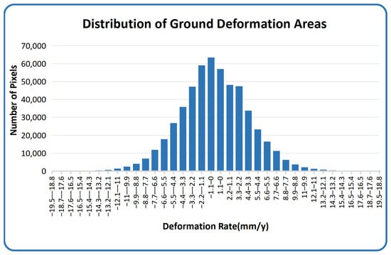
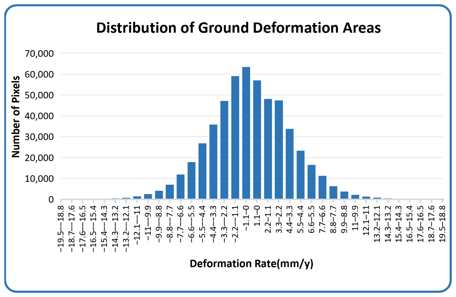
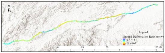
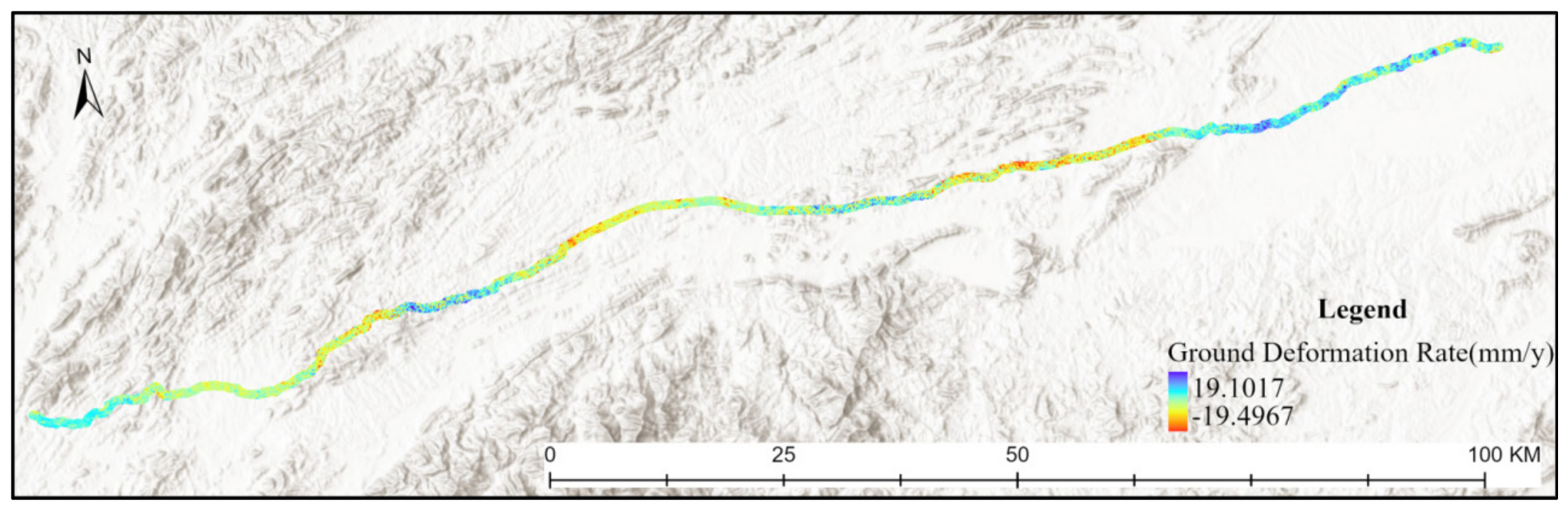
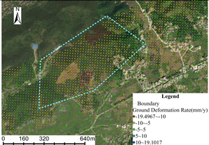
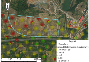
Ground deformation results are presented in Figure 5. The annual average deformation rate in the study area from 2021 to 2024 ranges from −19.5 to 19.1 mm/year. It should be noted that the deformation derived from SBAS-InSAR represents the displacement along the satellite line-of-sight (LOS), which is a combination of vertical and horizontal movements. Therefore, negative values do not strictly indicate pure subsidence, nor do positive values represent pure uplift. In this study, LOS deformation is used as an indicator of surface movement trends to identify potential deformation zones, rather than a direct measure of vertical displacement. In the absence of ascending and descending orbit data for decomposition, LOS measurements are commonly used in similar studies as a proxy for detecting surface deformation patterns. While the annual velocity values indicate the trend of ground stability, the primary threat to buried pipelines arises not from uniform uplift or subsidence alone, but from differential deformation across the pipeline corridor. High strain rates, occurring at the boundaries between subsiding and stable zones, induce bending and tensile stresses that may lead to pipe failure. As shown in Figure 7, areas of subsidence and uplift within the study region are approximately equal in extent and alternate spatially. A simple area statistics analysis shows that uplift and subsidence areas account for approximately 52.5% and 47.5% of the study area, respectively, indicating a relatively balanced spatial distribution. The data shown in Figure 8 are too complex for direct analysis, necessitating classification.
Figure 7.
Distribution of Ground Deformation Areas.
Figure 8.
Original ground deformation rate.
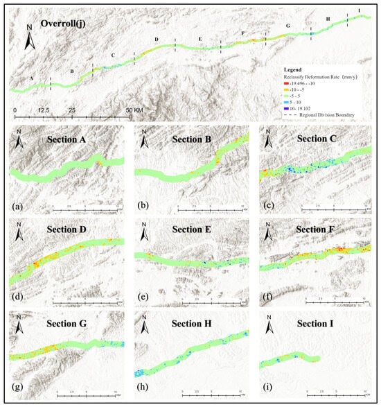
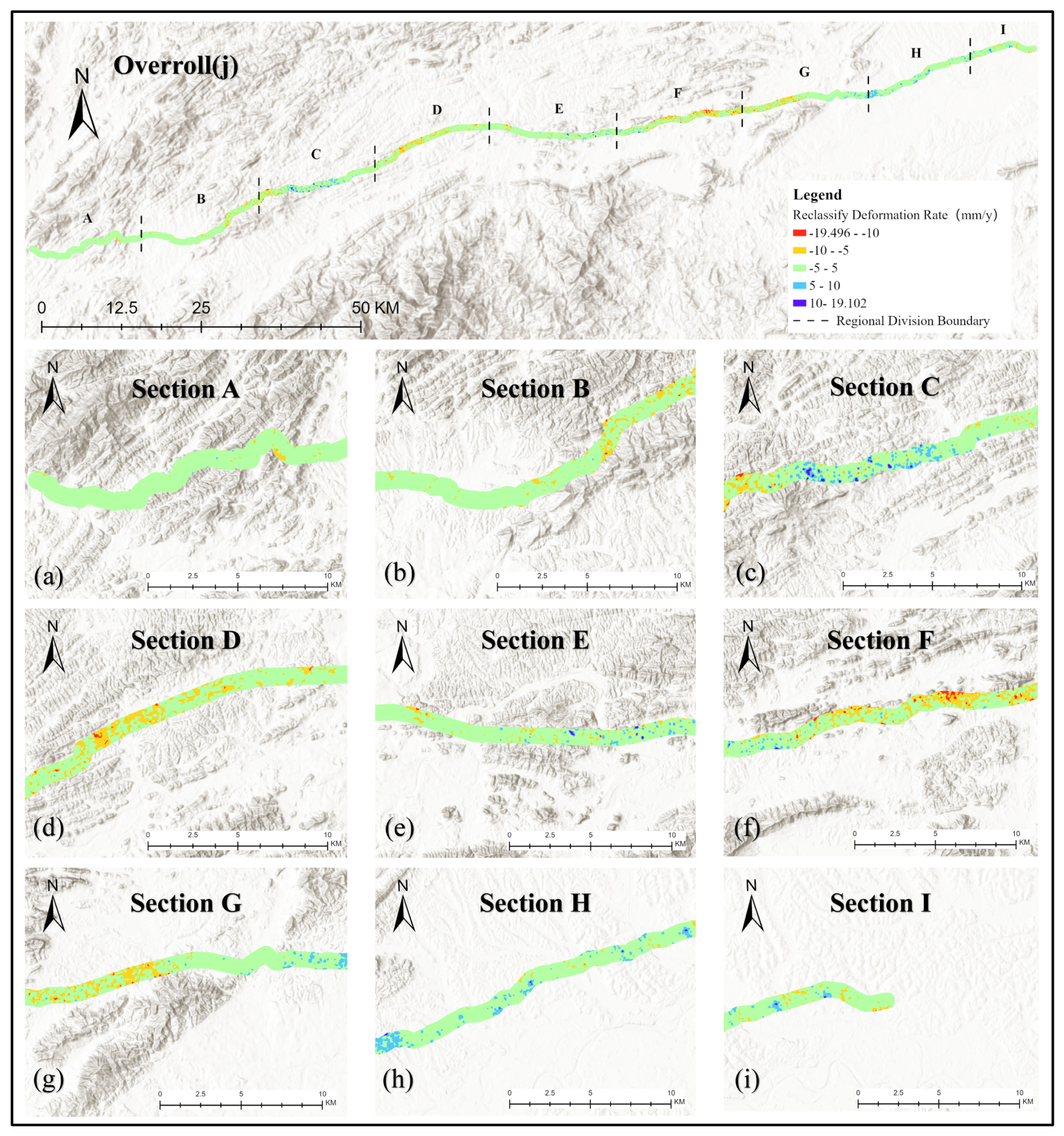
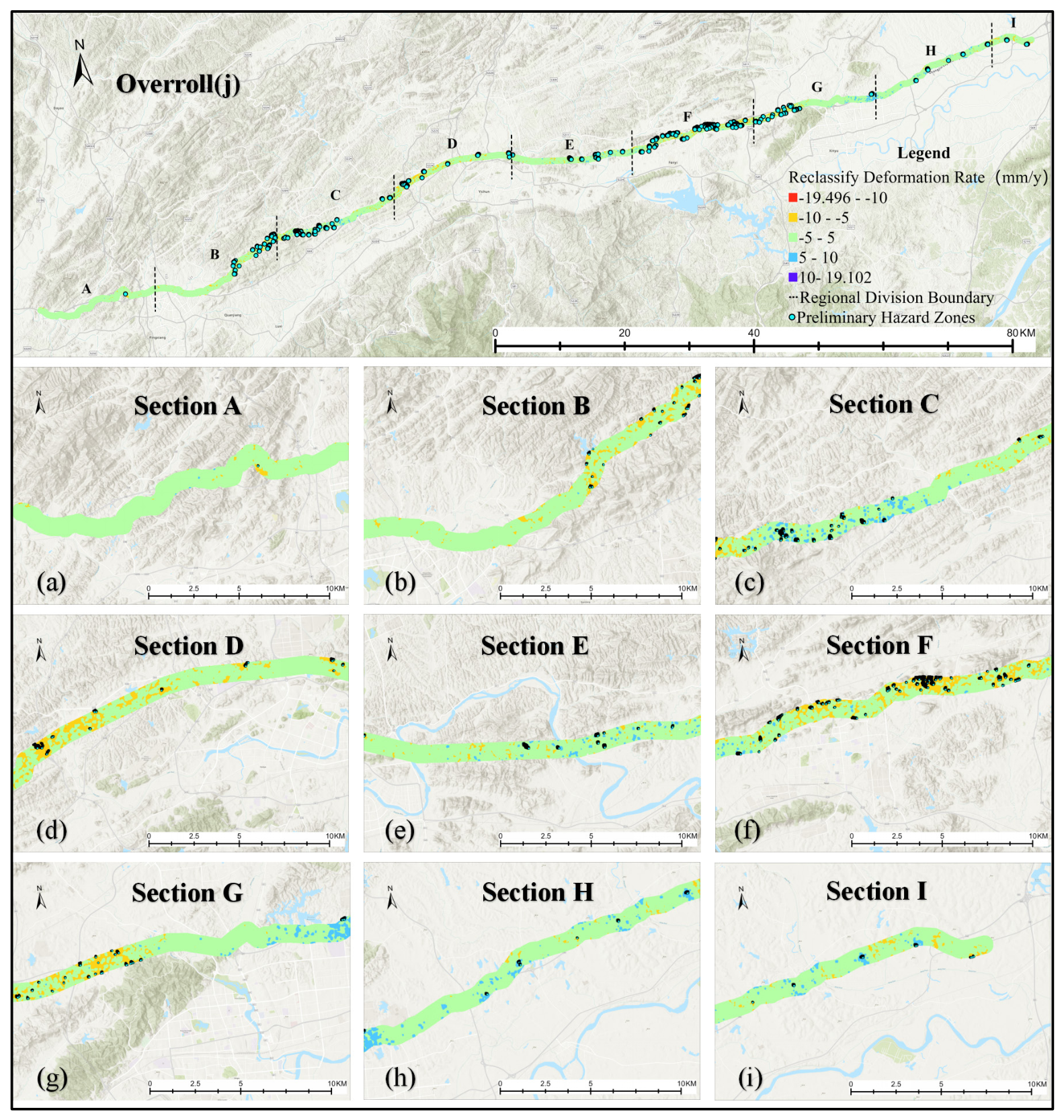
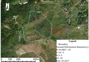
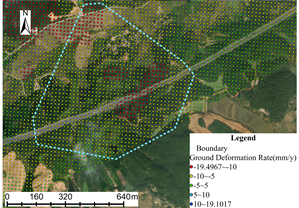
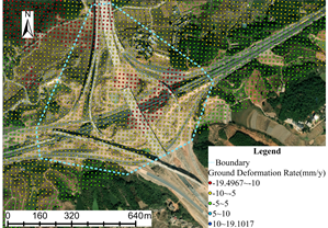
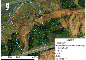
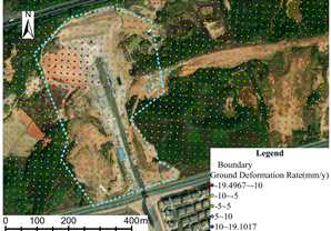
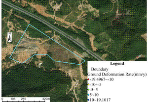
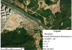
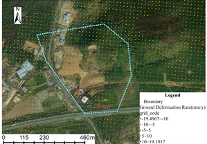
According to the Specifications for risk assessment of geological hazard [26], the deformation rate was classified into five categories: −19.5 to −10 mm/year, −10 to −5 mm/year, −5 to 5 mm/year, 5 to 10 mm/year, and 10 to 19.1 mm/year, with the classification results presented in Figure 9. The deformation thresholds used for hazard classification were determined based on a combination of previous studies, regional geological conditions, and empirical analysis of deformation distributions within the study area. These thresholds are commonly adopted in InSAR-based hazard identification studies and are considered effective for distinguishing significant deformation from background noise.
Figure 9.
Reclassify deformation rate. (a) Deformation rate of Section A; (b) Deformation rate of Section B; (c) Deformation rate of Section C; (d) Deformation rate of Section D; (e) Deformation rate of Section E; (f) Deformation rate of Section F; (g) Deformation rate of Section G; (h) Deformation rate of Section H; (i) Deformation rate of Section I; (j) Deformation rate of Overall.
Figure 9 indicates that ground deformation rates across the study area generally range between −5 mm/year and 5 mm/year, suggesting an overall relatively stable condition. A spatial association between high-deformation zones and highways or urban areas can be observed in some locations. However, this observation is qualitative and does not constitute a primary basis for the study’s conclusions. The main findings of this study rely on the integration of InSAR deformation, susceptibility assessment, and field verification. Notably, the Yichun–Fenyi section exhibits the most intense deformation, with rates exceeding ±10 mm/year and reaching up to ±20 mm/year in some localized areas. The distribution of high deformation rate zones is closely associated with topographic features and is mainly concentrated in three geomorphic units: transitional zones between low hills, hills, and plains; junctions between river terraces and alluvial plains; and areas surrounding urban development clusters. These areas generally exhibit complex geological conditions and frequent anthropogenic engineering activities, rendering them susceptible to significant surface deformation.
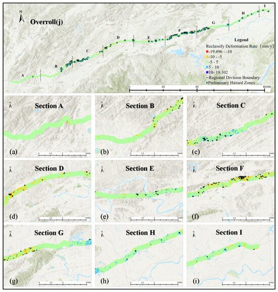
Rates from −19.5 to −10 mm/year and from 10 to 19.1 mm/year are identified as deformation-based potential hazard zones. In this study, deformation rates between −19.5 and −10 mm/year and between 10 and 19.1 mm/year were initially identified as potential disaster areas. It should be emphasized that deformation magnitude alone does not fully represent hazard risk, and therefore these zones are considered preliminary indicators rather than definitive hazard classifications. Preliminary analysis identified a total of 121 high-deformation-rate areas. A “high-deformation zone” is defined as a spatially continuous cluster of pixels exceeding the threshold, with a minimum mapping unit of 5 pixels. This threshold was chosen to reduce the influence of isolated noisy pixels and to ensure that the identified zones represent spatially coherent deformation patterns rather than random artifacts. These 121 high-deformation-rate zones were designated as preliminary geological hazard zones, as shown in Figure 10. Subsequently, the 121 preliminary geological hazard sites were screened by integrating the susceptibility assessment results and optical remote sensing imagery to improve the accuracy of hazard identification.
Figure 10.
Preliminary geological hazard zones. (a) Preliminary geological hazard zones of Section A; (b) Preliminary geological hazard zones of Section B; (c) Preliminary geological hazard zones of Section C; (d) Preliminary geological hazard zones of Section D; (e) Preliminary geological hazard zones of Section E; (f) Preliminary geological hazard zones of Section F; (g) Preliminary geological hazard zones of Section G; (h) Preliminary geological hazard zones of Section H; (i) Preliminary geological hazard zones of Section I; (j) Preliminary geological hazard zones of Overall.
3.2. Disaster Susceptibility Assessment
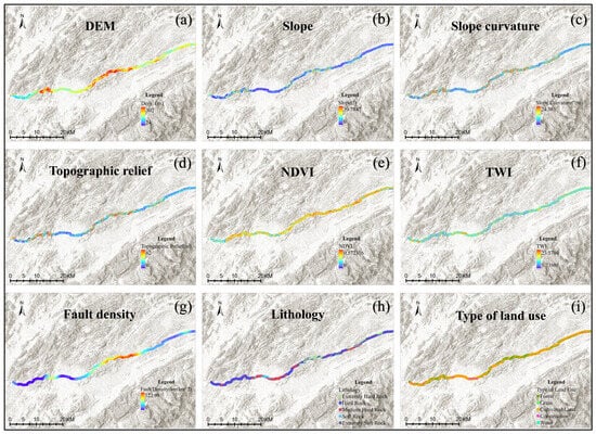
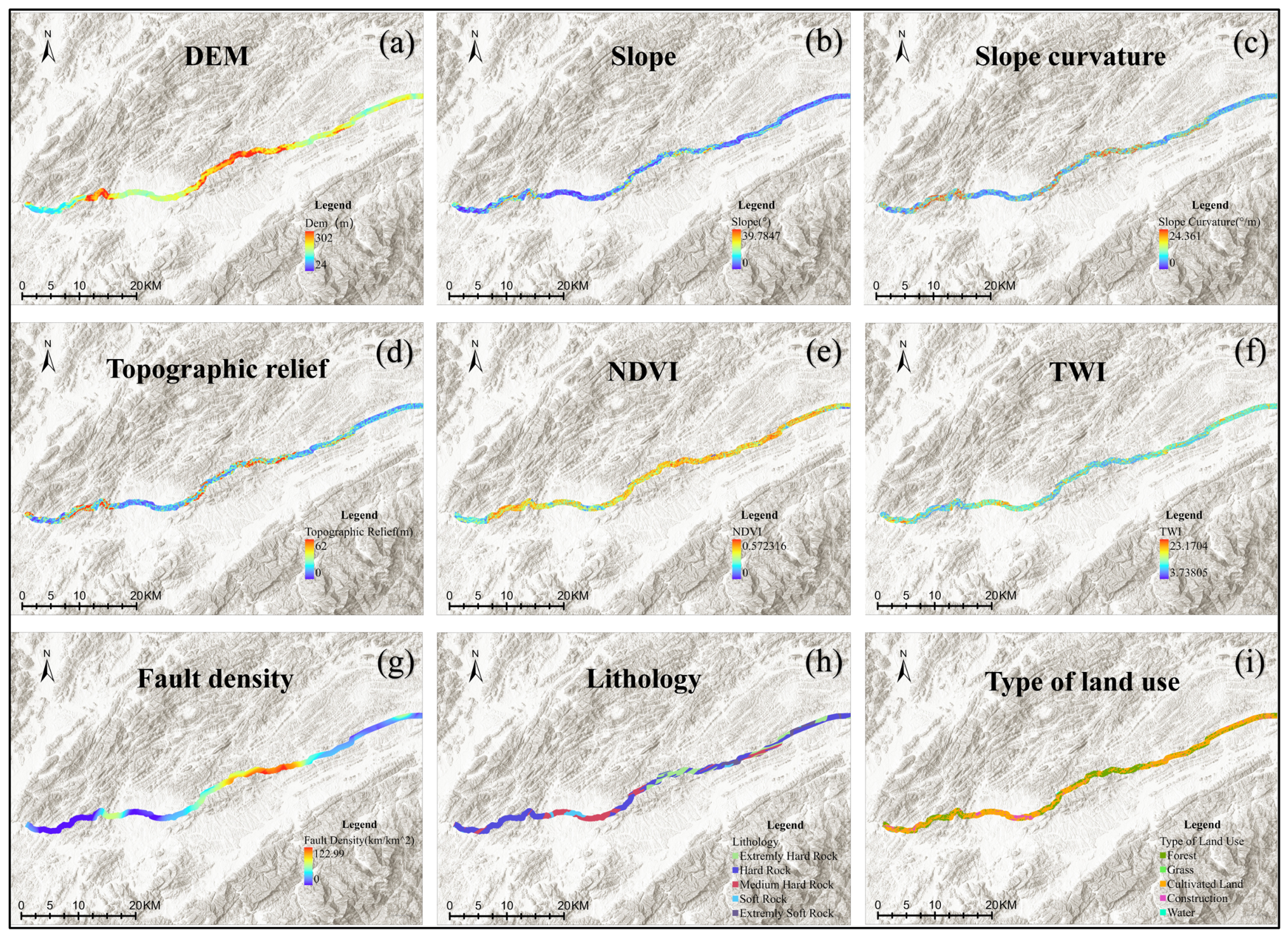
Geological disaster susceptibility in the study area was assessed using the information quantity method. Nine evaluation factors were selected for the analysis: elevation, slope, slope curvature, topographic relief, land use type, lithology, fault density, Terrain Wetness Index (TWI), and Normalized Difference Vegetation Index (NDVI), as shown in Figure 11.
Figure 11.
Evaluation factors.(a) DEM data of the study area; (b) Slope data of the study area; (c) Slope curvature data of the study area; (d) Topographic data of the study area; (e) NDVI data of the study area; (f) TWI data of the study area; (g) Fault density data of the study area; (h) Lithology data of the study area; (i) Land use data of the study area.
Each factor was assigned a grading value according to the classification table shown in Table 3. The grading and assignment values of each evaluation factor in this table are derived based on corporate standards and experience. The scoring is carried out for the index evaluation of common geological disaster types along oil and gas pipelines, and this grading system is only applicable to the geological hazard susceptibility evaluation of common onshore oil and gas transmission pipelines. Elevation data were obtained from a 30 m resolution digital elevation model (DEM), providing accurate topographic representation. Slope data were derived from GIS-based analysis of DEM data, effectively quantifying ground inclination. Slope curvature represents the rate of slope change and is critical for assessing geological disaster susceptibility. Topographic relief denotes the difference between the maximum and minimum elevations within a given area, illustrating terrain undulations. Land use type, derived from relevant planning documents, indicates that different land uses exert varying influences on the occurrence of geological disasters. Lithology data were obtained through geological surveys and data compilation. Considering the study area’s characteristics and previous research, the lithology was reclassified into extremely hard rock, hard rock, medium-hard rock, soft rock, and extremely soft rock, reflecting substantial differences in stability and erosion resistance. Fault density, calculated via GIS after mapping fault distributions, represents the concentration of faults within the study area. The Terrain Wetness Index (TWI) is a relative measure of surface water-holding capacity derived from DEM data [27]. It is calculated as a function of unit catchment area and surface slope [28], helping identify rainfall runoff patterns, potential soil moisture accumulation zones, and water pooling areas that may affect geological disaster occurrence. The Normalized Difference Vegetation Index (NDVI), calculated from red (absorbed by vegetation) and near-infrared (strongly reflected) wavelengths, reflects canopy density and dynamic changes in vegetation cover [29], providing a comprehensive assessment of regional vegetation conditions.
Table 3.
Reclassified evaluation factor.
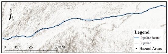
After obtaining classification scores for each evaluation index, their weights were determined using historical disaster data from the study area combined with the entropy weight method. These weights were subsequently applied to calculate geological disaster susceptibility. The distribution map of historical disaster sites is presented in Figure 12.
Figure 12.
Historical Disaster Sites.
The Entropy method was proposed by Shannon and Weaver in 1947 and further emphasized by Zeleny in 1982 [30]. Currently, the entropy method is the most commonly used objective method to determine the weights of criteria/constructs [31]. It establishes objective weights for attributes/responses by defining the importance of each response without considering the decision-makers’ preferences [30]. The Entropy measures the uncertainty of variables and evaluates how controlling factors influence outcomes [32]. It provides a quantitative measure of information content, allowing for the comparison and analysis of the effects of different statistical models, algorithms, and corresponding tuning parameters [33]. It is believed that the lower the entropy of a criterion, the more valuable information it contains [34]. This method has significantly influenced the modeling and mapping of various natural hazards [33]. The weights of the geological hazard indicators are shown in Table 4.
Table 4.
Weights of indicators.
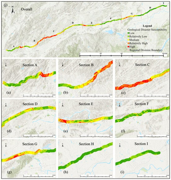
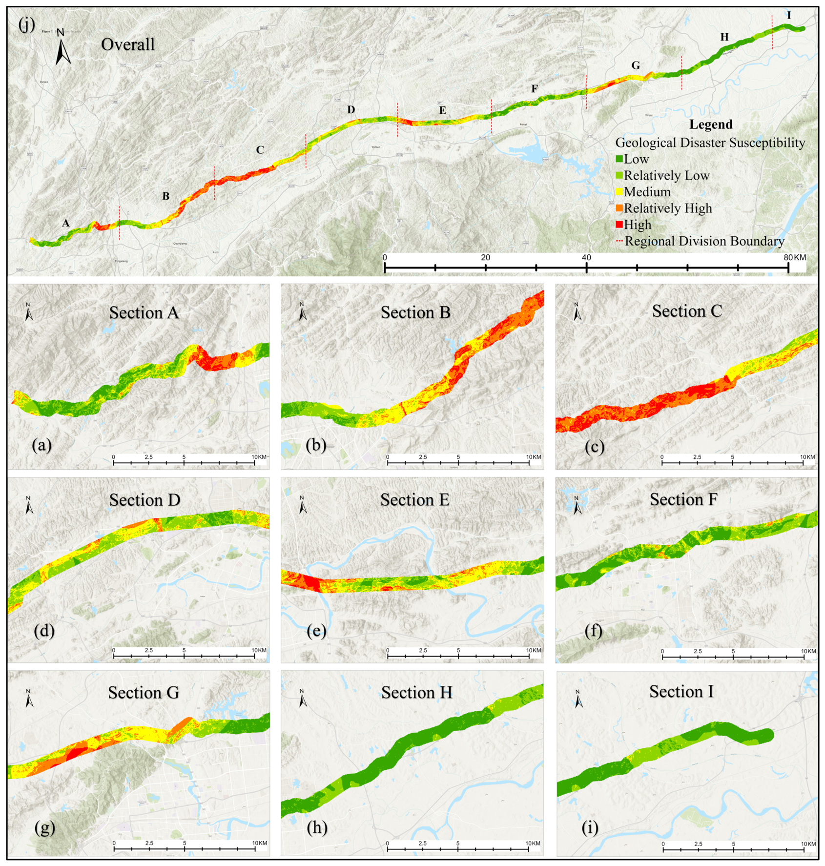
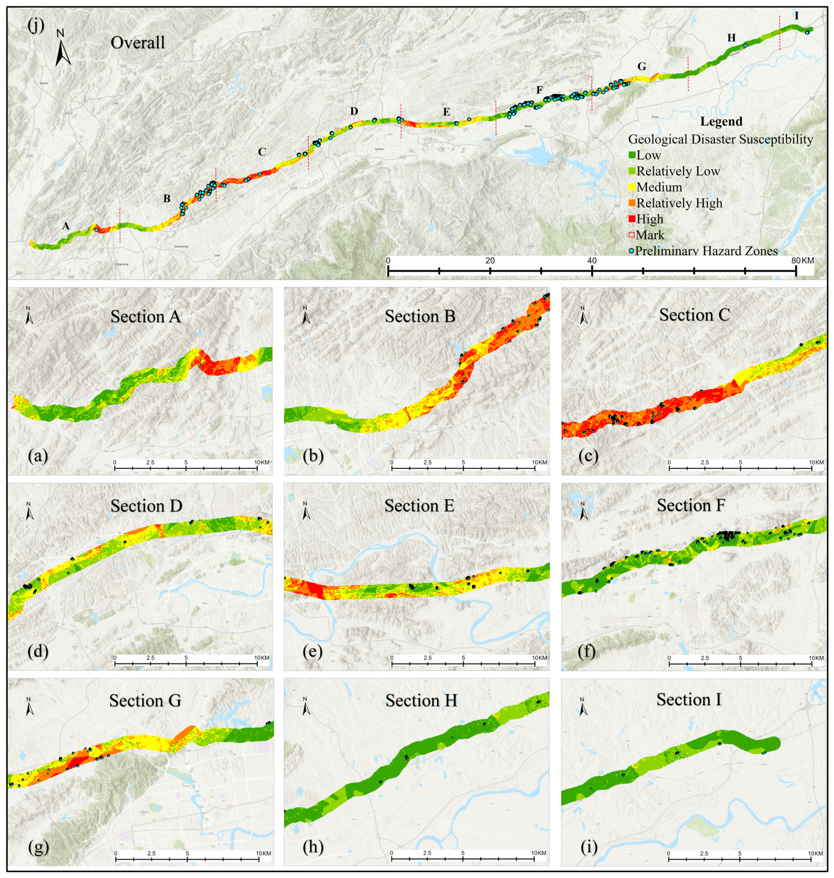
Entropy weight analysis indicates that slope curvature, fault density, and lithology significantly influence geological hazard susceptibility in the study area, each contributing over 10% to the total impact, with fault density accounting for a substantial 26.63%. By overlaying GIS layers of these indicators and applying the natural break method, susceptibility was classified into five levels: low, relatively low, moderate, relatively high, and high. The geological disaster susceptibility map of the study area is presented in Figure 13.
Figure 13.
Geological Disaster Susceptibility. (a) Disaster susceptibility of Section A; (b) Disaster susceptibility of Section B; (c) Disaster susceptibility of Section C; (d) Disaster susceptibility of Section D; (e) Disaster susceptibility of Section E; (f) Disaster susceptibility of Section F; (g) Disaster susceptibility of Section G; (h) Disaster susceptibility of Section H; (i) Disaster susceptibility of Section I; (j) Disaster susceptibility of Overall.
Figure 13 shows that the study area exhibits distinct geological hazard susceptibility patterns: sections B, C, and E along the assessment corridor display high or very high susceptibility, whereas sections G and I exhibit low susceptibility. These spatial patterns closely correspond with variations in key influencing factors, including fault density, slope curvature, and lithology. Using the information quantity method, nine critical factors were identified, and the entropy weight method confirmed fault density, lithology, and slope curvature as the primary determinants of susceptibility. The resulting five-level susceptibility zones delineate the spatial distribution of geological hazards, providing a foundation for regional identification and screening of geological disaster risks.
3.3. Comprehensive Comparison and Investigation
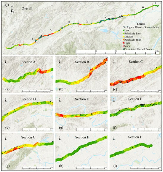
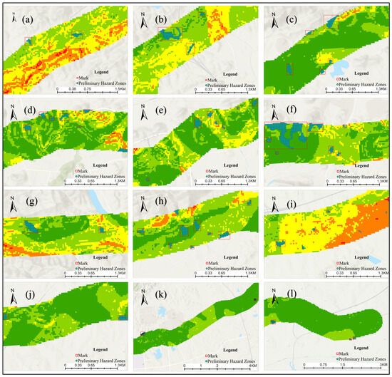
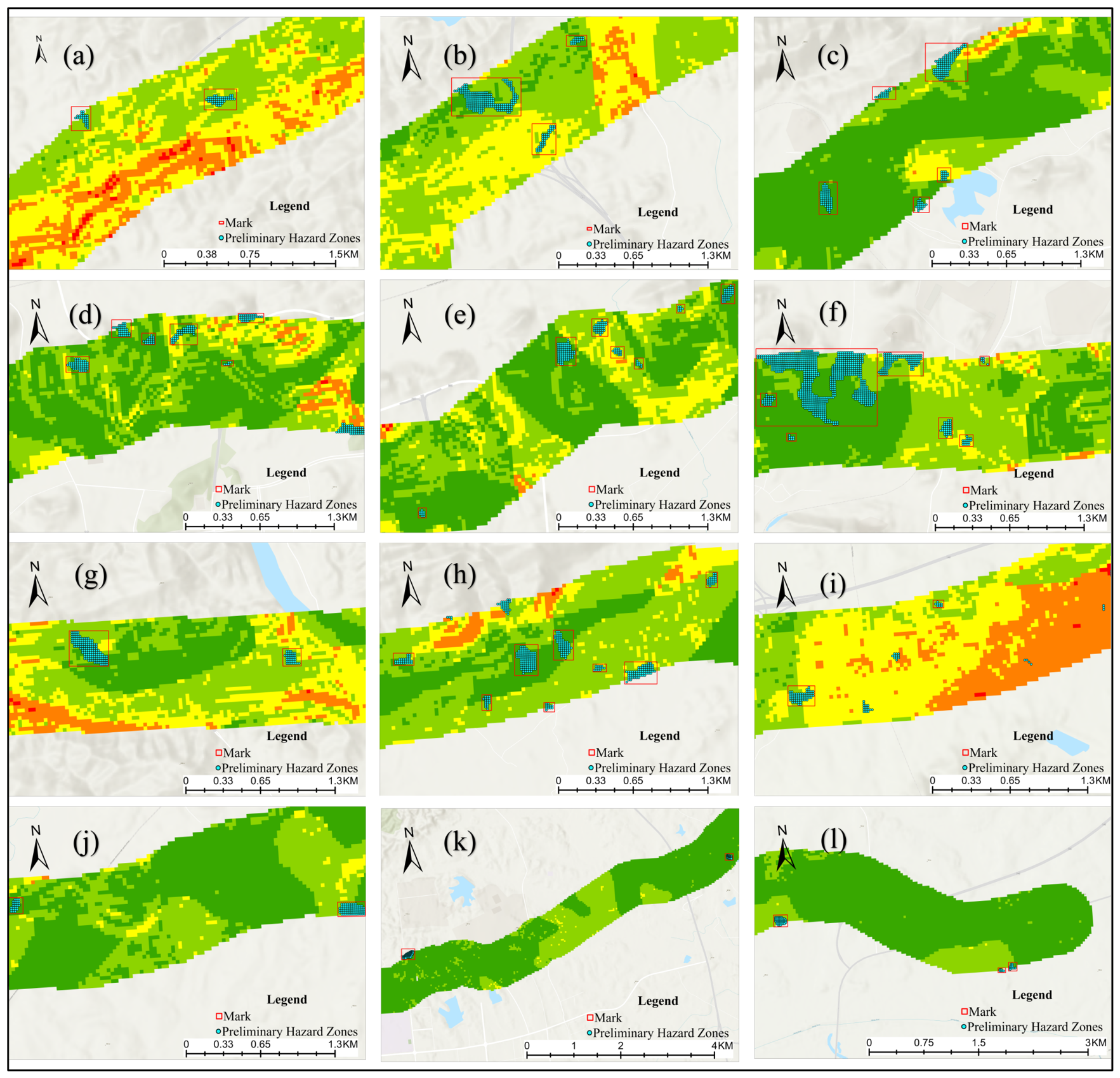
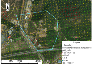
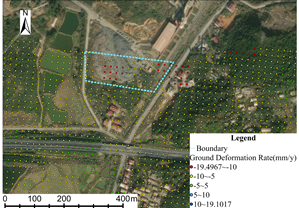
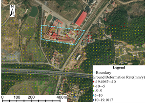
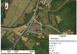
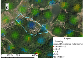
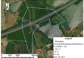
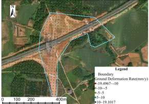
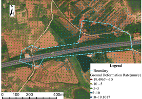
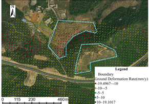
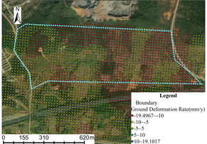
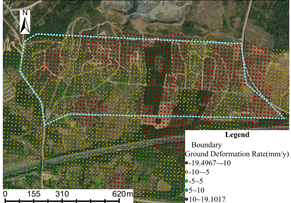
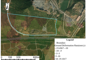
A systematic cross-comparison was performed by overlaying the 121 preliminary high-deformation zones derived from SBAS-InSAR onto the GIS-based geological disaster susceptibility map. As shown in Table 5, among the 121 preliminary zones, 75 were located within areas classified as “High” or “Relatively High” susceptibility, 18 within “Medium” susceptibility, and 28 within “Low” or “Relatively Low” susceptibility. As shown in Figure 14, blue circles indicate the preliminary geological hazard risk zones. Preliminary disaster assessment and vulnerability analysis for Areas D and F reveal notable discrepancies. Notably, in Area F, several preliminary disaster zones were identified despite its low vulnerability index. Zones identified as high-risk but located in areas of low susceptibility were marked and subsequently analyzed through visual interpretation of optical remote sensing images to assess their accuracy. The marked areas are presented in Figure 15. A total of 46 regions were marked for further analysis.
Table 5.
Distribution of the 121 preliminary disaster areas.
Figure 14.
Comprehensive Comparison. (a) Comprehensive comparison of Section A; (b) Comprehensive comparison of Section B; (c) Comprehensive comparison of Section C; (d) Comprehensive comparison of Section D; (e) Comprehensive comparison of Section E; (f) Comprehensive comparison of Section F; (g) Comprehensive comparison of Section G; (h) Comprehensive comparison of Section H; (i) Comprehensive comparison of Section I; (j) Comprehensive comparison of Overall.
Figure 15.
Marked zones. (a) Marked zones section 1; (b) Marked zones section 2; (c) Marked zones section 3; (d) Marked zones section 4; (e) Marked zones section 5; (f) Marked zones section 6; (g) Marked zones section 7; (h) Marked zones section 8; (i) Marked zones section 9; (j) Marked zones section 10; (k) Marked zones section 11; (l) Marked zones section 12.
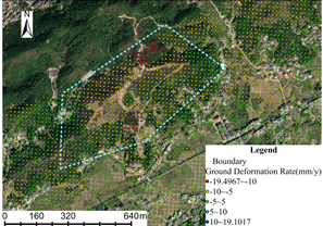
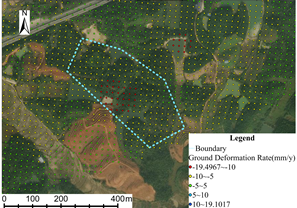
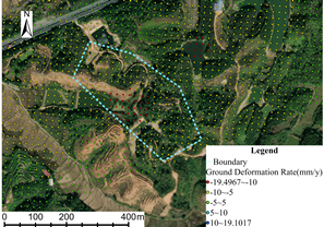
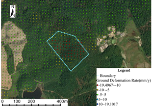
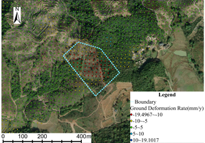
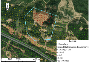
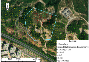
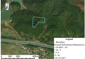
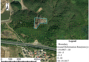
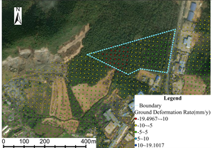
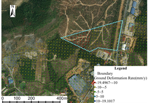
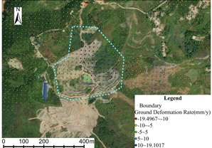
Optical remote sensing imagery from the World Imagery Wayback website was used for visual screening. By comparing images from January 2021 and December 2024 within the study area, preliminary disaster sites misclassified due to human activities were identified, particularly in the marked areas. Unlike an individual identification of each preliminary disaster site, markers of human activity were more distinct, leading to improved recognition accuracy and higher efficiency. These areas were broadly categorized into three types: civil buildings, cultivated land reclamation, and forest land loss. As shown in Table 6, of the 46 discordant points in low-susceptibility zones, 21 were false alarms from human activity; the remaining 25 represented active hazards missed by the static GIS model, highlighting InSAR’s complementary role.
Table 6.
List of human activity areas.
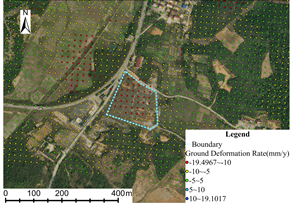
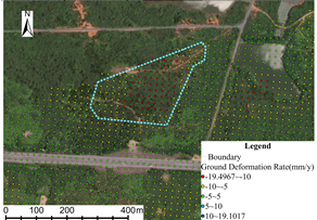
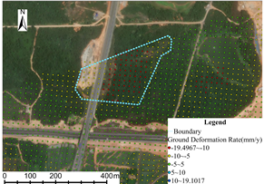
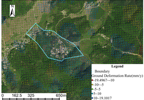
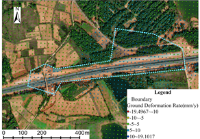
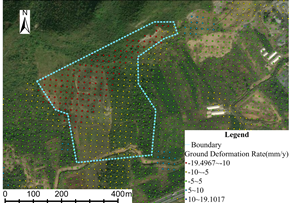
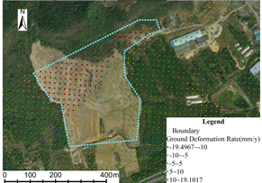
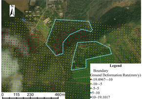
After excluding the 21 human activity sites, a total of 100 preliminary geological hazard sites were retained. On-site verification and investigation were conducted for these sites. This verification phase served as a critical field validation and provided information enrichment for the preliminary indoor interpretation results. Field verification was not merely a simple “map comparison” but a core process that translated indoor remote sensing macro-identification results into on-site micro-evidence, integrating geological expertise for comprehensive diagnosis. It provided indispensable field evidence and enhanced understanding for the subsequent scientific formulation of monitoring and early warning plans, risk management measures, and engineering governance designs. A brief example of representative InSAR hazard sites from field verification is presented in Table A1 of the Appendix A.
In the preliminary identification of geological hazard sites, initial assessments of potential locations and disaster types were conducted, followed by accuracy verification via field surveys. A total of 100 pre-identified geological hazard sites in the research area were systematically examined, resulting in the identification of 78 actual disaster sites. The field investigation form is presented in Table A2 of the Appendix A. As shown in Table 7, based on the field-verified dataset, the proposed framework achieved a precision of 78.0%, corresponding to a commission error of 22.0%. It should be acknowledged that the current validation design does not permit calculation of recall or omission error, as a systematic randomized survey of areas classified as “low deformation” by InSAR was beyond the logistical scope of this field campaign. Consequently, the false negative rate remains unquantified. Nevertheless, for the operational purpose of prioritizing pipeline inspections, precision is arguably the more critical metric, as a high false alarm rate would undermine confidence and waste inspection resources. Future monitoring cycles will incorporate a stratified random sampling protocol to enable construction of a complete confusion matrix and comprehensive performance evaluation.
Table 7.
Distribution of the 46 discordant points.
This result provides robust technical support for hazard identification, monitoring, and early warning. However, the progression from “suspected deformation” to “actual disaster” involves substantial uncertainties. The technology cannot directly predict the timing or scope of future disasters, but rather indicates areas with higher probabilities of disaster occurrence, characterized by significant cumulative deformation and rapid deformation rates over extended periods. Therefore, adopting a collaborative approach, integrating multi-source data, and implementing continuous monitoring in key regions are essential for establishing a disaster deformation database. This approach enhances capabilities from early identification to monitoring and early warning, ultimately supporting disaster prevention and mitigation efforts.
4. Discussion
4.1. Limitation of the Study
The Sentinel-1A satellite data used in this study has a ground resolution of 5 × 20 m, which is insufficient for detecting small-scale hidden disasters with widths of less than 10 m. Additionally, the study area, located in a subtropical monsoon climate zone, experiences high vegetation coverage and dense cloud cover during the rainy season, which can lead to SAR image coherence loss. Atmospheric phase residuals may further compromise the accuracy of deformation inversion in localized areas, including valleys and riverbanks. The foundational data, encompassing stratigraphic lithology and geological structures, rely on historical records, such as 1:200,000 regional geological maps. The land use classification data, derived from the 2020 version, does not account for recent surface changes induced by human engineering activities, such as road expansions and farmland development around pipelines. Furthermore, the susceptibility assessment incorporates only nine static geological environmental factors, lacking dynamic indicators, such as real-time precipitation intensity, extreme weather events, and human activity levels. Consequently, the static nature of the evaluation limits its ability to effectively address short-term triggers of geological hazards. The study focuses on identifying individual hazard points and assessing single disasters, without systematically analyzing the chain reactions of geological hazards. The susceptibility assessment incorporates only nine static geological environmental factors, lacking dynamic indicators such as real-time precipitation intensity, extreme weather events, and human activity levels. Consequently, the static nature of the evaluation limits its ability to effectively address short-term triggers of geological hazards.
Furthermore, the precision of the InSAR-based screening reaches 78.0%, but the omission error remains unknown. Field verification targeted only detected anomalies; random sampling in stable-appearing areas was not conducted. Hence, slow-moving hazards with deformation below C-band detection limits or obscured by decorrelation cannot be ruled out. Furthermore, the single-geometry LOS measurement precludes separation of vertical and horizontal motion components.
In addition, the identification of hazard points and the classification of deformation levels rely partly on manually established empirical thresholds. However, the selection of influencing factors and their classification still involve certain empirical considerations. Although these choices are supported by previous studies and regional characteristics, they may introduce subjectivity into the assessment results.
It should be acknowledged that several of the limitations discussed above, such as C-band decorrelation in vegetated terrain and the inherent ambiguity of single-geometry LOS measurements, are well recognized challenges in the InSAR community and do not represent novel findings of this study. However, rather than simply restating these known issues, the present work addresses them operationally through the proposed multi-source integration framework. The combination of InSAR-derived deformation rates with GIS-based susceptibility mapping provides a practical means of filtering geologically irrelevant signals, including those arising from decorrelation noise. Similarly, while LOS measurements cannot be decomposed without additional orbital geometries, their utility as a screening tool for differential deformation is demonstrated here, particularly when interpreted alongside susceptibility zones and optical imagery. True methodological advances that fundamentally overcome these limitations, such as L-band or S-band SAR for improved coherence, multi-orbit decomposition for three-dimensional displacement retrieval, and dynamic susceptibility modeling with near-real-time environmental forcing, remain important directions for future work. These are elaborated further in the following section.
4.2. Prospects
In terms of visual interpretation, by combining high-precision remote sensing technologies, such as unmanned aerial vehicle (UAV) surveying and LiDAR, with SBAS-InSAR data, centimeter-level terrain and object information can be obtained, thereby enhancing the detection capability for small-scale concealed disasters. At the same time, by using deep learning algorithms including convolutional neural networks and Transformers, integrating InSAR deformation data, optical image texture features, and terrain factors, an end-to-end automated identification model is constructed to minimize the subjectivity of manual interpretation. For example, an innovative deep learning model, SCGC-Net, is specifically designed for landslide detection in multi-source remote sensing images. It combines CNN and Mamba (an advanced class of Transformer architecture) to extract global and local features, and integrates various factors such as terrain and optical texture, achieving high-precision end-to-end automated recognition [35]. Also, a method combining SBAS-InSAR technology with the spatio-temporal graph convolutional network (STGCN, a deep learning model) was proposed for long-term panoramic prediction of landslides. The study utilized SBAS-InSAR to obtain deformation history and combined it with UAV surveys for verification, aiming to enhance the prediction capability for complex landslides [36].
In terms of susceptibility assessment, by integrating real-time precipitation data from meteorological stations, hydrological flow data, and soil moisture monitoring data around pipelines, a dynamic vulnerability assessment database can be constructed to achieve real-time updates of assessment results. This system integrates assessment factors such as ground motion parameters, human engineering activity intensity, and pipeline characteristics, and uses a disaster chain coupling model to simulate the combined impact of multiple disasters, thereby comprehensively reflecting the comprehensive risk posed by disasters to pipelines. For example, Correa-Calle et al. developed a dynamic model for landslide threats, specifically designed to assess the risks faced by the OCENSA oil pipeline in Colombia. This model integrates satellite remote sensing daily rainfall data from the NASA Global Precipitation Measurement (GPM) mission, enabling continuous monitoring of meteorological conditions [37].
In terms of the automation of the identification process, machine learning algorithms such as random forests and gradient boosting trees are used instead of the traditional entropy weight method, achieving data-driven automatic optimization of indicator weights and reducing reliance on human experience. By combining Bayesian probability models with InSAR deformation rates, GIS vulnerability grades, and field survey data, a quantitative model is constructed to quantify the probability of disaster occurrence and pipeline damage risk, thereby achieving refined risk classification. For example, Gao et al. proposed a method of optimizing the Bayesian network by integrating SBAS-InSAR surface deformation data, which significantly improved the accuracy of landslide susceptibility assessment [38].
Future research should further improve the integration and automation of the proposed framework. In particular, the incorporation of deep learning methods may help reduce the subjectivity associated with manual interpretation and enable more efficient identification of hazard features from multi-source remote sensing data. At the same time, introducing dynamic environmental factors such as real-time precipitation, soil moisture, and human activity intensity would allow susceptibility assessment to better reflect short-term triggering conditions. In addition, more robust and data-driven approaches are needed to determine deformation thresholds and factor weights, thereby enhancing the objectivity and reproducibility of the model. Expanding field validation datasets and long-term monitoring records would also contribute to improving the reliability and generalization capability of the framework.
5. Conclusions
This study developed an integrated framework combining SBAS-InSAR deformation monitoring with GIS-based susceptibility modeling for the early identification of geological hazards along the Xiangtan Connection Line of the West–East Gas Pipeline. The principal conclusions are as follows:
- (1)
- SBAS-InSAR analysis revealed that surface deformation along the pipeline corridor is generally stable, with high-deformation zones concentrated in transitional geomorphic units and areas of soft lithology, which correspond closely with the geohazard susceptibility zones derived from the GIS model.
- (2)
- Fault density, lithology, and slope curvature were identified as the primary factors governing geological hazard susceptibility in the study area, providing a quantitative basis for prioritizing pipeline sections for risk mitigation.
- (3)
- Multi-source verification—combining optical remote sensing interpretation and field reconnaissance—confirmed a high consistency rate between satellite-derived anomalies and actual geohazards, demonstrating that the proposed framework effectively filters anthropogenic noise and enhances the reliability of early hazard identification.
The integrated SBAS-InSAR–GIS approach offers a practical and efficient alternative to conventional manual patrols, enabling pipeline operators to transition from reactive maintenance to proactive risk management in geologically complex corridors. Future research will focus on incorporating high-resolution topographic data and real-time meteorological variables to further refine the dynamic assessment of pipeline geohazard risks.
Author Contributions
Conceptualization, X.R. and M.G.; methodology, M.G. and J.L.; software, M.G. and Z.L.; validation, J.A. and Z.L.; formal analysis, J.L.; investigation, J.A. and M.G.; resources, X.R.; data curation, M.G.; writing—original draft preparation, M.G.; writing—review and editing, X.R. and J.L.; visualization, M.G.; supervision, X.R.; project administration, X.R. and J.A.; funding acquisition, X.R. All authors have read and agreed to the published version of the manuscript.
Funding
This research was funded by the National Natural Science Foundation of China (42372319).
Institutional Review Board Statement
Not applicable.
Informed Consent Statement
Not applicable.
Data Availability Statement
The data presented in this study are available on request from the corresponding author. The data are not publicly available due to some of the data contain company confidential information.
Conflicts of Interest
Author Jian Ai was employed by the Nanchang Gas Delivery Branch of China National Oil & Gas Pipeline Network Corporation’s West-East Gas Pipeline Company. Author Zhongdi Liu was employed by the Hefei Gas Delivery Branch of China National Oil & Gas Pipeline Network Corporation’s West-East Gas Pipeline Company. The remaining authors declare that the research was conducted in the absence of any commercial or financial relationships that could be construed as a potential conflict of interest.
Appendix A
Table A1.
Example of representative geological hazard zone.
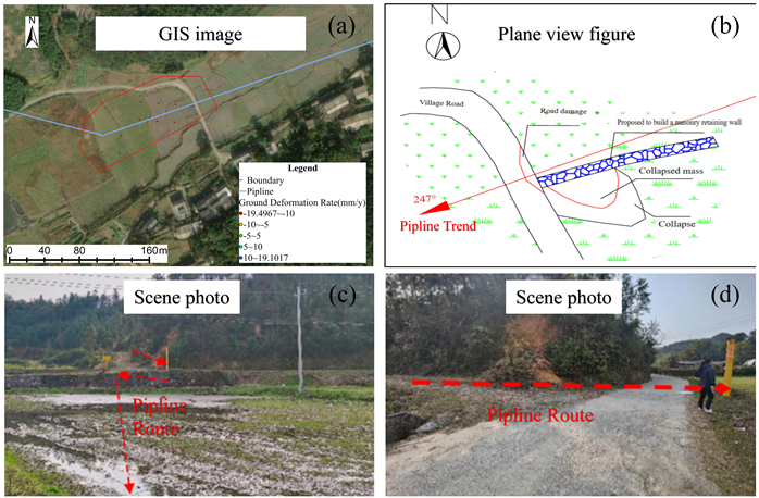
Table A2.
Field site verification.
References
- Yang, Y.; Liu, Y.; Guo, Y.; Shen, J.; Xie, C.; Zhang, N.; Tian, B.; Zhu, Y.; Mao, Y. An InSAR-Based Framework for Advanced Large-Scale Failure Probability Assessment of Oil and Gas Pipelines. Remote Sens. 2025, 17, 504. [Google Scholar] [CrossRef] [Scilit]
- He, B.; Bai, M.; Shi, H.; Li, X.; Qi, Y.; Li, Y.; He, B.; Bai, M.; Shi, H.; Li, X.; et al. Risk Assessment of Pipeline Engineering Geological Disaster Based on GIS and WOE-GA-BP Models. Appl. Sci. 2021, 11, 9919. [Google Scholar] [CrossRef] [Scilit]
- Deng, Q.; Fu, M.; Ren, X. Does Pipelaying Method Affect the Development of Pipeline Geohazards and Maintenance Cost? A Case Study of Zhongxian-Wuhan Gas Pipeline, China. Bull. Eng. Geol. Environ. 2020, 79, 97–107. [Google Scholar] [CrossRef] [Scilit]
- Jin, B.; Zeng, T.; Wang, T.; Zhang, Z.; Gui, L.; Yin, K.; Zhao, B. Advanced Risk Assessment Framework for Land Subsidence Impacts on Transmission Towers in Salt Lake Region. Environ. Model. Softw. 2024, 177, 106058. [Google Scholar] [CrossRef] [Scilit]
- Shahriar, A.; Sadiq, R.; Tesfamariam, S. Risk Analysis for Oil & Gas Pipelines: A Sustainability Assessment Approach Using Fuzzy Based Bow-Tie Analysis. J. Loss Prev. Process Ind. 2012, 25, 505–523. [Google Scholar] [CrossRef] [Scilit]
- Fang, H.; Shao, Y.; Xie, C.; Tian, B.; Zhu, Y.; Guo, Y.; Yang, Q.; Yang, Y.; Fang, H.; Shao, Y.; et al. Using Persistent Scatterer Interferometry for Post-Earthquake Landslide Susceptibility Mapping in Jiuzhaigou. Appl. Sci. 2022, 12, 9228. [Google Scholar] [CrossRef] [Scilit]
- Shen, C.; Feng, Z.; Xie, C.; Fang, H.; Zhao, B.; Ou, W.; Zhu, Y.; Wang, K.; Li, H.; Bai, H.; et al. Refinement of Landslide Susceptibility Map Using Persistent Scatterer Interferometry in Areas of Intense Mining Activities in the Karst Region of Southwest China. Remote Sens. 2019, 11, 2821. [Google Scholar] [CrossRef] [Scilit]
- Hakim, W.L.; Fadhillah, M.F.; Park, S.; Pradhan, B.; Won, J.-S.; Lee, C.-W. InSAR Time-Series Analysis and Susceptibility Mapping for Land Subsidence in Semarang, Indonesia Using Convolutional Neural Network and Support Vector Regression. Remote Sens. Environ. 2023, 287, 113453. [Google Scholar] [CrossRef] [Scilit]
- Berardino, P.; Fornaro, G.; Lanari, R.; Sansosti, E. A New Algorithm for Surface Deformation Monitoring Based on Small Baseline Differential SAR Interferograms. IEEE Trans. Geosci. Remote Sens. 2002, 40, 2375–2383. [Google Scholar] [CrossRef] [Scilit]
- Hussain, M.A.; Chen, Z.; Khan, J. Monitoring Land Subsidence in the Peshawar District, Pakistan, with a Multi-Track PS-InSAR Technique. Environ. Sci. Pollut. Res. 2024, 31, 12271–12287. [Google Scholar] [CrossRef] [Scilit]
- Tong, X.; Schmidt, D. Active Movement of the Cascade Landslide Complex in Washington from a Coherence-Based InSAR Time Series Method. Remote Sens. Environ. 2016, 186, 405–415. [Google Scholar] [CrossRef] [Scilit]
- Yingying, L.; Changcheng, G.; Yunfu, Z. Comprehensive Review of Evaluation Methods for Geological Disaster Susceptibility. Geol. Resour. 2024, 33, 65–73. [Google Scholar] [CrossRef]
- Ai-di, H.; Hui-xia, Z.; Li, Z.; Hua, L.; Ming, H. A Sampled Method of Classification of Susceptibility Evaluation Unit for Geological Hazards Based on GIS. Appl. Math. Inf. Sci. 2012, 6, 19–23. [Google Scholar]
- Guzzetti, F.; Mondini, A.C.; Cardinali, M.; Fiorucci, F.; Santangelo, M.; Chang, K.-T. Landslide Inventory Maps: New Tools for an Old Problem. Earth-Sci. Rev. 2012, 112, 42–66. [Google Scholar] [CrossRef] [Scilit]
- Reichenbach, P.; Rossi, M.; Malamud, B.D.; Mihir, M.; Guzzetti, F. A Review of Statistically-Based Landslide Susceptibility Models. Earth-Sci. Rev. 2018, 180, 60–91. [Google Scholar] [CrossRef] [Scilit]
- Pradhan, B. Remote Sensing and GIS-Based Landslide Hazard Analysis and Cross-Validation Using Multivariate Logistic Regression Model on Three Test Areas in Malaysia. Adv. Space Res. 2010, 45, 1244–1256. [Google Scholar] [CrossRef] [Scilit]
- Zhenda, W.; Yue, T.; Xinyi, H.; Ming, G.; Yaxuan, W.; Ruoxin, W.; Jiangjihong, C. Space-Air-Ground Remote Sensing-Based Spatial Database Design for Cultivated Land Monitoring Integrated with InSAR Analysis. Sci. Prog. 2025, 108, 00368504251391263. [Google Scholar] [CrossRef] [Scilit]
- Cao, C.; Zhu, K.; Xu, P.; Shan, B.; Yang, G.; Song, S. Refined Landslide Susceptibility Analysis Based on InSAR Technology and UAV Multi-Source Data. J. Clean. Prod. 2022, 368, 133146. [Google Scholar] [CrossRef] [Scilit]
- Tizzani, P.; Berardino, P.; Casu, F.; Euillades, P.; Manzo, M.; Ricciardi, G.; Zeni, G.; Lanari, R. Surface Deformation of Long Valley Caldera and Mono Basin, California, Investigated with the SBAS-InSAR Approach. Remote Sens. Environ. 2007, 108, 277–289. [Google Scholar] [CrossRef] [Scilit]
- Liu, X.; Xing, X.; Wen, D.; Chen, L.; Yuan, Z.; Liu, B.; Tan, J.; Liu, X.; Xing, X.; Wen, D.; et al. Mining-Induced Time-Series Deformation Investigation Based on SBAS-InSAR Technique: A Case Study of Drilling Water Solution Rock Salt Mine. Sensors 2019, 19, 5511. [Google Scholar] [CrossRef] [Scilit]
- Yang, W.; Niu, R.; Si, R.; Li, J.; Yang, W.; Niu, R.; Si, R.; Li, J. Geological Hazard Susceptibility Analysis and Developmental Characteristics Based on Slope Unit, Using the Xinxian County, Henan Province as an Example. Sensors 2024, 24, 2457. [Google Scholar] [CrossRef] [Scilit]
- Alatza, S.; Papoutsis, I.; Paradissis, D.; Kontoes, C.; Papadopoulos, G.A.; Alatza, S.; Papoutsis, I.; Paradissis, D.; Kontoes, C.; Papadopoulos, G.A. Multi-Temporal InSAR Analysis for Monitoring Ground Deformation in Amorgos Island, Greece. Sensors 2020, 20, 338. [Google Scholar] [CrossRef] [Scilit] [PubMed]
- Shan, B.; Qi, J.; Tian, W.; Zhu, K.; Jin, T.; Yang, Q.; An, X.; Yang, G.; Hu, Q.; Cao, C.; et al. Early Identification of Geological Hazards Along the Power Transmission Line in Weinan Based on SBAS-InSAR. Appl. Sci. 2025, 15, 920. [Google Scholar] [CrossRef] [Scilit]
- Lu, Z.; Yang, H.; Zeng, W.; Liu, P.; Wang, Y. Geological Hazard Identification and Susceptibility Assessment Based on MT-InSAR. Remote Sens. 2023, 15, 5316. [Google Scholar] [CrossRef] [Scilit]
- Song, Q.; Sun, B.; Gao, X.; Liu, Y. Laboratory Investigation on the Influence of Factors on the Outflow Temperature from Stratified Reservoir Regulated by Temperature Control Curtain. Environ. Sci. Pollut. Res. 2020, 27, 33052–33064. [Google Scholar] [CrossRef] [Scilit]
- GB/T 40112—2021; Specifications for Risk Assessment of Geological Hazard. Ministry of Natural Resources of the People’s Republic of China: Beijing, China, 2021.
- Beven, K.J.; Kirkby, M.J. A Physically Based, Variable Contributing Area Model of Basin Hydrology/Un Modèle à Base Physique de Zone d’Appel Variable de l’hydrologie Du Bassin Versant. Hydrol. Sci. Bull. 1979, 24, 43–69. [Google Scholar] [CrossRef] [Scilit]
- Wang, H.; Han, G.; Xie, X. Dan liu xiang fa di xing shi du zhi shu chi du xiao ying de bu tong di xing qu cha yi fen xi [Scale effect of the topographic wetness index based on the single flow direction method across different terrain regions]. Geogr. Geo-Inf. Sci. 2016, 32, 23–29. [Google Scholar]
- Gamon, J.A.; Field, C.B.; Goulden, M.L.; Griffin, K.L.; Hartley, A.E.; Joel, G.; Peñuelas, J.; Valentini, R. Relationships Between NDVI, Canopy Structure, and Photosynthesis in Three Californian Vegetation Types. Ecol. Appl. 1995, 5, 28–41. [Google Scholar] [CrossRef] [Scilit]
- Kumar, R.; Bilga, P.S.; Singh, S. Multi Objective Optimization Using Different Methods of Assigning Weights to Energy Consumption Responses, Surface Roughness and Material Removal Rate during Rough Turning Operation. J. Clean. Prod. 2017, 164, 45–57. [Google Scholar] [CrossRef] [Scilit]
- Teixeira, S.J.; Ferreira, J.; Wanke, P.; Antunes, J.J.M. Evaluation Model of Competitive and Innovative Tourism Practices Based on Information Entropy and Alternative Criteria Weight. Tour. Econ. 2021, 27, 23–44. [Google Scholar] [CrossRef] [Scilit]
- Ziarh, G.F.; Asaduzzaman, M.; Dewan, A.; Nashwan, M.S.; Shahid, S. Integration of Catastrophe and Entropy Theories for Flood Risk Mapping in Peninsular Malaysia. J. Flood Risk Manag. 2021, 14, e12686. [Google Scholar] [CrossRef] [Scilit]
- Hansen, T.M. Entropy and Information Content of Geostatistical Models. Math. Geosci. 2021, 53, 163–184. [Google Scholar] [CrossRef] [Scilit]
- Mukhametzyanov, I. Specific Character of Objective Methods for Determining Weights of Criteria in MCDM Problems: Entropy, CRITIC and SD. Decis. Mak. Appl. Manag. Eng. 2021, 4, 76–105. [Google Scholar] [CrossRef] [Scilit]
- Fan, Y.; Ma, P.; Hu, Q.; Liu, G.; Guo, Z.; Tang, Y.; Wu, F.; Zhang, H. SCGC-Net: Spatial Context-Guided Calibration Network for Multisource RSI Landslides Detection. IEEE Trans. Geosci. Remote Sens. 2025, 63, 5400817. [Google Scholar] [CrossRef] [Scilit]
- Li, Z.; Chen, J.; Cao, C.; Zhang, W.; Zhu, K.; Bai, J.; Wu, C. Enhancing Long-Term Prediction of Non-Homogeneous Landslides Incorporating Spatiotemporal Graph Convolutional Networks and InSAR. Eng. Geol. 2025, 347, 107917. [Google Scholar] [CrossRef] [Scilit]
- Correa-Calle, O.; Botía-Díaz, M.; García-Orozco, F.; Quintero-Londoño, J. Development of the Dynamic Model of Mass Movements Threat for the Corridor of the Central Oil Pipeline S.A., “OCENSA” in the Framework of the Management of the Climate and External Forces Threat. In Proceedings of the 2024 15th International Pipeline Conference. Volume 4: Geohazards Management and Strain-Based Design and Assessment; American Society of Mechanical Engineers: New York, NY, USA, 2024. [Google Scholar]
- Gao, X.; Wang, B.; Dai, W.; Liu, Y. A Landslide Susceptibility Assessment Method Using SBAS-InSAR to Optimize Bayesian Network. Front. Environ. Sci. 2025, 13, 1522949. [Google Scholar] [CrossRef] [Scilit]

Disclaimer/Publisher’s Note: The statements, opinions and data contained in all publications are solely those of the individual author(s) and contributor(s) and not of MDPI and/or the editor(s). MDPI and/or the editor(s) disclaim responsibility for any injury to people or property resulting from any ideas, methods, instructions or products referred to in the content. |
© 2026 by the authors. Licensee MDPI, Basel, Switzerland. This article is an open access article distributed under the terms and conditions of the Creative Commons Attribution (CC BY) license.