New Insights into How the Rupture Radius of Deep Fault Rupture Affects the Magnitude of Induced Earthquakes

Abstract

Underground fluid injection is regarded as one of the important factors inducing seismic activity. This study therefore proposes a method to predict the maximum damage area and seismic magnitude induced by fluid injection, in order to quantify the relationship between stress disturbances in faults and induced seismic activity during fluid injection. This method involves analysing a three-dimensional geological model of fault permeability evolution in order to define the seismic rupture zone of faults during fluid injection projects. It also involves calculating the maximum damage area and seismic magnitude induced by injection and verifying the method’s effectiveness using field data. The results show that, during deep injection, continuous injection of fluid reduces the effective stress on the fault and increases the fracture area. Following the sudden cessation of injection, the rupture area and maximum seismic magnitude reach their peak values. During the initial stage of injection, seismic magnitude increases rapidly with the rupture radius of the fault, while the growth rate of seismic magnitude decreases during the stable injection stage. Once injection has ceased, the rupture range and seismic magnitude will gradually stabilise throughout the entire geological self-balancing stage. Periodic injection results in the largest fault rupture area, whereas linear growth injection induces the highest seismicity. Strike-slip faults exhibit the most significant increase in rupture area, whereas normal faults demonstrate more intense seismicity evolution. Low permeability, proximity to injection wells and direct well closure exacerbate instability, whereas linear slow closure is the safest option. These research results can inform seismic risk management in fluid injection engineering.

1. Introduction

Every year, numerous seismic events occur worldwide. While the vast majority are natural earthquakes, the remaining seismic events are related to human activities [1,2], such as injection-induced earthquakes [3,4,5]. Moreover, with the rapid increase in the number and scale of underground engineering projects globally in recent years, the number of induced seismic events associated with various human engineering activities has been rising year by year [1,6,7,8].

The large-scale injection of fluids underground can alter the stress on faults, potentially reactivating pre-existing dormant faults or faults in a critical stress state [9,10,11,12]. As a result, underground fluid injections are considered one of the significant factors contributing to induced seismicity [2,7,13]. Fluid injection-induced earthquakes hinder the rapid development of Earth’s energy systems, such as carbon dioxide geological storage [14,15,16] and hydraulic stimulation in enhanced geothermal systems [17,18].

In previous studies, both experimental and theoretical research have explored the source mechanisms of fluid injection-induced seismicity, which can be summarized into three types. The first type occurs when injected fluids reach a fault, increasing the pore pressure on the fault and reducing its frictional shear strength, thereby triggering fault instability and inducing seismic activity [19,20,21,22,23,24,25]. The second type involves fluid injection altering the stress field near the fault, affecting its stress state and ultimately inducing earthquakes [26,27,28,29]. The third type arises when fluid injection causes aseismic slip in the rock mass near the injection zone, which destabilizes a critically stressed fault far from the injection well, leading to seismic activity [21]. Based on the analysis of these three source mechanisms, researchers have proposed various corresponding fluid injection strategies and seismic prediction methods to reduce the likelihood of induced earthquakes in injection projects [3,30,31]. However, most studies have primarily focused on the fault’s response to pore pressure changes caused by injection or have separately analyzed the mechanisms of induced seismicity at different stages of fluid injection, without comprehensively considering the evolution of the entire stress field on the fault due to fluid injection [3,30,31,32]. For example, there has been insufficient examination of the spatiotemporal correlation of induced seismicity during and after well shut-in, the influence of effective stress evolution on the timing and likelihood of such seismic events, or the prediction of earthquake magnitudes and stress perturbation ranges caused by fluid injection.

Deep fluid injection projects can induce stress perturbations on faults and trigger seismic activity; research on forecasting the rupture zone and magnitude of induced earthquakes remains limited. Existing induced seismicity models are largely confined to predicting the physical mechanisms of injection-induced earthquakes based solely on pore pressure changes along faults. However, in reality, seismic events triggered by stress-enhanced zones within underground reservoirs and faults due to fluid injection can propagate into surrounding regions. If these propagating seismic waves reach fault areas with accumulated elastic energy capable of initiating new ruptures, those zones may also undergo stress perturbations, further triggering seismic ruptures and expanding the rupture range of injection-induced earthquakes [33,34,35,36]. Nevertheless, previous theoretical models for estimating the maximum magnitude of induced earthquakes have largely overlooked the relationship between earthquake magnitude and the triggering stress perturbations [37,38,39].

This study focuses on the evolutionary characteristics of fault stress fields and establishes a theoretical scaling relationship between the maximum magnitude of fluid-injection-induced earthquakes and the resulting stress changes along the fault. A theoretical estimation method has been developed to calculate the maximum rupture size caused by local stress perturbations along a fault and the maximum seismic magnitude resulting from such disturbances. This method was validated through simulations using a constructed 3D geological model. The study evaluated the effects of various factors—including fluid injection rates, fault locations, well-to-fault distances, fault types, reservoir permeability, and shut-in strategies—on the maximum rupture extent and the triggered maximum earthquake magnitude. Additionally, the proposed method of calculating the maximum seismic magnitude induced by fluid injection was employed to analyse the spatial and temporal distribution of seismic data along faults in the Bend Arch Fort Worth Basin near Johnson County, Texas.

2. Theoretical Model

2.1. Fluid Structure Coupling Mathematical Model Equation

During the water injection process, the deformation control equation of the reservoir is:

$$G{u}_{i,kk}+{\displaystyle \frac{G}{1-2v}}{u}_{k,ki}=f_i+{\alpha }_f{p}_f$$

(1)

where u represents displacement, p_f denotes pore pressure, α_f is the Biot coefficient, and G is the shear modulus, f_i is the gravitational coefficient, m/s². The subscripts i and k indicate the three directional components of the variables, where i, k = 1, 2, 3 follows the Einstein summation convention, and the comma denotes differentiation with respect to the variable.

The fluid mass balance equation primarily consists of the rate of fluid mass change, fluid mass flux, and mass source term:

$${\displaystyle \frac{\partial m_f}{\partial t}}+\nabla \cdot J_f=Q_s$$

(2)

where J_f represents the fluid mass flux within the reservoir, and Q_s represents the mass source–sink term. The default fluid is stored in the voids of the reservoir in a free state:

$$m_f={\rho }_f{\varphi }_f$$

(3)

where φ_f is the porosity of the reservoir, and ρ_f is the fluid density in the reservoir. This article also considers the compression characteristics of fluids, where fluid density varies with the volume of fluid compression. Therefore, fluid density can be expressed as:

$${\rho }_f={\displaystyle \frac{1}{C_f}}{\displaystyle \frac{\mathrm{d}{\rho }_f}{\mathrm{d}{p}_f}}$$

(4)

where c_f is the compressibility coefficient of the fluid.

The fluid mass flux J_f can be expressed as:

$$J_f={\displaystyle \frac{k_f}{{\mu }_f}}{\rho }_f(\nabla p_f+{\rho }_{f}g)$$

(5)

where k_f is the permeability in the reservoir, μ_f f is the dynamic viscosity coefficient of the fluid, and g is the gravitational acceleration. In the coupled model, changes in fluid quality are related to changes in reservoir pore pressure and reservoir deformation:

$${\displaystyle \frac{\partial m_f}{\partial t}}={\displaystyle \frac{1}{M}}{\displaystyle \frac{\partial p_f}{\partial t}}+{\alpha }_f{\displaystyle \frac{\partial {\epsilon }_V}{\partial t}}$$

(6)

Among them, M represents Biot modulus, and ε_V represents volumetric strain.

2.2. Calculation Method for Regional Earthquake Magnitude and Fracture Radius Induced by Fluid Injection in Oil Fields

The injection of large volumes of fluids into the subsurface triggers a coupled hydro-mechanical process that can reactivate critically stressed or dormant faults, leading to induced seismicity. Prior to fluid injection, the fault is subjected to an initial tectonic shear stress τ₀ and an initial effective normal stress σ₀. As fluid injection proceeds, the increase in pore pressure causes a redistribution of stress conditions along the fault. Simultaneously, fluid injection elevates pore pressure within the reservoir, thereby reducing the fault’s shear strength, expressed as μ(σ_n − p), where μ is the friction coefficient, (σ_n − p) is the normal stress, and p is pore pressure. When the shear strength drops below the fault’s shear stress, the fault undergoes unstable slip. To estimate the extent of the maximum impact zone caused by stress disturbances resulting from water injection, this study assumes that the fault was initially locked during the early stress adjustment phase. Only when the stress on the fault reaches the critical instability condition does the fault slip in a single seismic event, releasing accumulated stress. The magnitude of the resulting earthquake is then calculated based on this rupture process.

2.2.1. Seismic Rupture Radius

The maximum earthquake arrest area serves as a stability evaluation metric during fault stress perturbation processes. When injected fluids diffuse through the reservoir and reach the fault along permeable damage zones, they induce localized stress perturbations, triggering stress redistribution on the fault. As fluid injection continues, the area of stress perturbation on the fault expands. However, the stress perturbation caused by injection attenuates with the growth of the fault’s unstable rupture area, while the influence of tectonic stress on the fault increases accordingly. Therefore, the extent of unstable rupture on the fault is generally governed by the competing effects between the fault’s original tectonic stress and the stress redistribution induced by fluid pressurization. These two factors reach equilibrium at the boundary of the maximum earthquake arrest area.

The background stress drop Δτ of a fault is composed of its original structural shear stress and original structural effective stress:

$$∆\tau ={\tau }_0-\mu ({\sigma }_{n0}-p_{f0})$$

(7)

where τ₀ represents the fault’s initial tectonic shear stress, σ_n0 denotes the fault’s original tectonic normal stress, and p_f0 indicates the fault’s initial pore pressure. The potential stress drop on the fault can be expressed as the excess of fault shear stress over the fault’s shear strength after stress perturbation induced by injection. Its specific equation is given by:

$$∆\tau ={\tau }_0-\mu (∆{\sigma }_n-∆p_f)$$

(8)

where Δσ_n represents the change in normal stress on the fault induced by injection-driven stress perturbation, and Δp_f denotes the corresponding change in pore pressure on the fault. Following fluid injection, the additional stress drop at the fault-reservoir interface caused by effective stress evolution can be approximated as:

$$F=\mu (∆{\sigma }_n-∆p_f)A$$

(9)

where A represents the area of the fault’s destabilized rupture zone (A = πr², r denoting the radius of the perturbed unstable rupture region). The additional stress drop at the fault-reservoir interface, induced by effective stress evolution, can be approximated as a point load superimposed on the fault’s background stress drop. This is expressed as follows:

$$∆\tau \left(r\right)=∆{\tau }_0+F\delta \left(r\right)/L$$

(10)

where δ(r) is the local slip at the fault interface, m; L represents the boundary span of the fault’s destabilized rupture zone, via., L = 2πr.

Based on the Griffith crack equilibrium criterion and yield fracture mechanics criterion, and given the spatial distribution of potential stress drop, according to the research of Galis et al. [36], an equation for calculating the area of unstable fracture induced by injection on a fault is derived. Simplify the calculation model of earthquake stopping area using the following assumptions: (1) The unstable rupture area on the fault is roughly circular with a radius of r. (2) The additional stress drop caused by the effective stress evolution caused by injection on the fault is distributed in an axisymmetric manner, and the point load superimposed on the background stress drop of the fault is assumed to be Δτ(r). (3) The average static stress intensity factor at the boundary of the unstable fracture zone along the fault is approximately expressed as a tensile (Type I) crack in the Griffith crack equilibrium criterion of fracture mechanics. Its specific form is:

$$K_0\left(R\right)={\displaystyle \frac{2}{\sqrt{\pi r}}}{\int }_0^R{\displaystyle \frac{∆\tau \left(r\right)}{\sqrt{R^2-r^2}}}rdr$$

(11)

where the adopted definition of the polar coordinate Dirac delta function conforms to the following computational expression:

$${\int }_0^R\delta \left(r\right)rdr$$

(12)

In fracture mechanics, according to the Griffith crack equilibrium criterion, the fracture toughness K_c is related to the slip-weakening fracture energy. The condition for unstable rupture on a fault can be expressed as:

$$K_0\left(R\right)=K_c$$

(13)

$${\displaystyle \frac{\partial (K_0-K_c)}{\partial r}}<0$$

(14)

Among these, the first condition is that the stress conditions on the fault satisfy the Griffith crack equilibrium criterion in fracture mechanics, and the second condition is that the stable equilibrium condition of the fault is met, meaning that under this equilibrium, further stress perturbations on the fault will not lead to another rupture. According to the stress intensity factor K₀(R) of the crack, the stress drop affects the fault’s arrest zone under the following three scenarios. (1) If the region influenced by the injection-induced stress perturbation is too small, the rupture will not propagate beyond the stress-perturbed zone because the stress intensity factor K₀ induced by the perturbation does not reach the fracture toughness K_c. (2) If the perturbation is sufficiently large, it can trigger runaway rupture on the fault, because once the stress intensity factor K₀ exceeds the fracture toughness K_c, the unstable rupture zone on the fault will continue to expand. (3) The intermediate case is when the rupture propagates beyond the stress-perturbed zone but stops upon reaching stable equilibrium, i.e., when the stress intensity factor K₀ equals the fracture toughness K₀.

By approximating the additional stress drop (Equation (10)) induced by the effective stress evolution on the fault as a point load Δτ(r) superimposed on the background stress drop and substituting it into the Mode I crack failure criterion (Equation (11)), we can obtain:

$$K_0\left(R\right)={\displaystyle \frac{F}{{\left(\pi R\right)}^{\frac{3}{2}}}}+2∆{\tau }_0\sqrt{{\displaystyle \frac{R}{\pi }}}$$

(15)

In Equation (15), the first term decreases as the rupture arrest radius r increases, while the second term increases with r. Therefore, the stress intensity factor K₀(r) of the crack has a single minimum value. Runaway rupture on the fault can only occur if this minimum stress intensity factor exceeds the fracture toughness K_c. By solving the Griffiths equilibrium condition (Equation (11)), an expression for the maximum rupture containment radius R_max induced by fault stress disturbances caused by water injection can be derived, which takes the form:

$$R_{max}=\sqrt{{\displaystyle \frac{3F}{2\pi ∆{\tau }_0}}}=\sqrt{{\displaystyle \frac{3\mu ∆{\sigma }_{n}A}{2\pi ∆{\tau }_0}}}$$

(16)

Based on the derived expression for the maximum rupture arrest radius R_max induced by injection-triggered stress perturbations on the fault, it can be concluded that fault rupture is governed by the competition between two types of elastic energy: the effective stress evolution on the fault caused by injection and the tectonic pre-stress on the fault.

2.2.2. Earthquake Magnitude

The magnitude of the moment of an earthquake, M_w, can be expressed as:

$$M_w={\displaystyle \frac{2}{3}}{log}_{10}{M}_0-6.07$$

(17)

where M₀ represents the seismic moment, and its specific form can be expressed as:

$$M_0={\displaystyle \frac{16}{7}}∆{\tau }_0{r}^3$$

(18)

Among them, r is the fault-stopping radius caused by injection. Substituting the maximum fracture radius r_max (Equation (16)) into the expressions for seismic moment and seismic magnitude yields:

$$M_0=2.29{∆{\tau }_0}^{-{\displaystyle \frac{1}{2}}}{\left({\displaystyle \frac{3\mu ∆{\sigma }_{n}A}{2\pi }}\right)}^{{\displaystyle \frac{3}{2}}}$$

(19)

$$M_w=1.52{∆{\tau }_{0}log}_{10}{\left({\displaystyle \frac{3\mu ∆{\sigma }_{n}A}{2\pi ∆{\tau }_0}}\right)}^{{\displaystyle \frac{3}{2}}}-6.07$$

(20)

3. Saltwater Wastewater Treatment Project near Venus, Texas

Between 2008 and 2015, a significant year-by-year increase in seismic activity was detected near Venus, Texas, USA. The largest recorded events included a magnitude 4.0 earthquake in 2015 [40,41]. This frequent seismicity appears closely correlated with brine/wastewater injection operations that began in 2006. Field monitoring data revealed that seismic events progressively migrated to greater depths along the fault over time, exhibiting a delayed response where significant seismic signals continued to be detected even after well shutdown [42].

This section will establish a numerical model capable of accurately reflecting the stratigraphic characteristics of the Venus area in Texas, to be used for simulating and validating the detected seismic signals. The model aims to elucidate the coupled fluid flow-geomechanical mechanisms responsible for induced seismicity and explain the underlying causes of the high-frequency earthquake occurrence.

3.1. Numerical Models

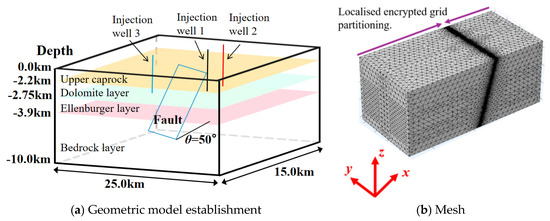
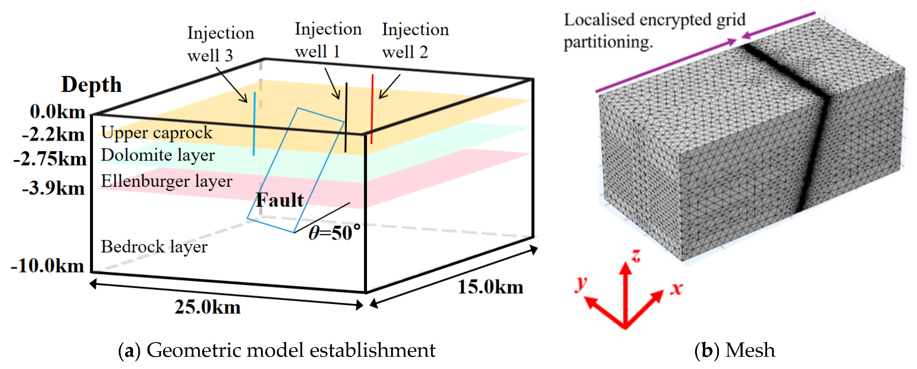
Based on seismic monitoring data from the SWD (saltwater disposal) operation near Venus, Texas [42,43,44], a rectangular geological system measuring 25 km long, 15 km wide, and 10 km high was constructed. The modeled geological system comprises four strata: a 2.2 km upper caprock, a 0.55 km dolomite layer, a 1.15 km highly permeable Ellenburger formation, and a 6.1 km bedrock layer, along with a normal fault system. The fault system consists of a low-permeability fault core flanked by damage zones on both sides. As shown in Figure 1a, consistent with field conditions at the Venus SWD site, the fault is modeled in a normal faulting stress regime with a 50° dip towards the Y-direction. To address potential mesh convergence issues caused by significant scale variations, the grid was refined towards the fault to ensure a smooth transition from meter-scale to kilometer-scale resolution (Figure 1b). The final discretized model contains 659,818 tetrahedral elements and 1,128,607 hexahedral elements, with an average element quality of 0.5302. The highly permeable Ellenburger formation serves as the reservoir, with three injection wells positioned at 1.0 km, 1.5 km, and 2.0 km from the fault. The wells at 1.0 km and 1.5 km are located on the fault’s footwall, while the 2.0 km-distant well is situated on the hanging wall. Following actual field monitoring data, six observation points were selected along the fault strike within the bedrock layer’s damage zones on both sides of the fault to analyze seismic magnitude data in the simulation.

Figure 1. Three-dimensional geological model that includes cap rocks, faults, reservoirs, and bedrock.

3.2. Stress and Boundary Conditions

This section uses the “Solid Mechanics” and “Darcy’s Law” modules in COMSOL Multiphysics (Version 5.4) to perform fluid–structure interaction simulations of deformation and fluid flow in faults and geological formations. The base of the geological model was fixed with zero displacement in all coordinate directions, while the top surface was set as a free deformation boundary with zero displacement constraints. Three injection wells were introduced into the reservoir, with all lateral boundaries configured as no-flow boundaries. To simulate the normal faulting stress regime, the three principal stresses were defined as follows: vertical stress (σ_v) = 35 MPa, maximum horizontal principal stress (σ_Hmax) = 24.5 MPa, and minimum horizontal principal stress (σ_hmin) = 22.4 MPa. The initial pore pressure in the reservoir was set at 2.0 MPa. Table 1 presents the complete set of parameters selected based on the hydrogeological characteristics observed at the Venus, Texas SWD site [42,43,44].

Table 1. Property Parameters of Simulation Model.

Symbol	Parameter	Value	Unit
kCover layer	Cover layer permeability	1.88 × 10−13	m2
kMarble	Marble permeability	1.00 × 10−17	m2
kBarnett	Barnett layer permeability	1.00 × 10−20	m2
kEllenburger	Ellenburger layer permeability	2.96 × 10−14	m2
kB	Permeability of bedrock	1.00 × 10−19	m2
kf	Fault permeability	2.49 × 10−15	m2
E	Young’s modulus	2.0 × 1010	Pa
Φm	porosity	0.20	-
υ	Poisson’s ratio	0.25	-

4. Model Results and Discussion

Using the fluid injection process established for unconventional oil and gas extraction in the previous chapter as a representative case study, this study predicts the seismic blocking radius and magnitude of regional seismic events triggered by injection in oilfields. In addition, the study investigates the relationship between the evolution of the critical stiffness of injection-induced faults and the seismic blocking radius as well as the seismic moment.

4.1. Evolution of Seismic Rupture Radius Induced by Fluid Injection

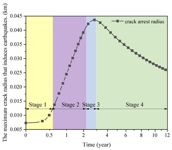
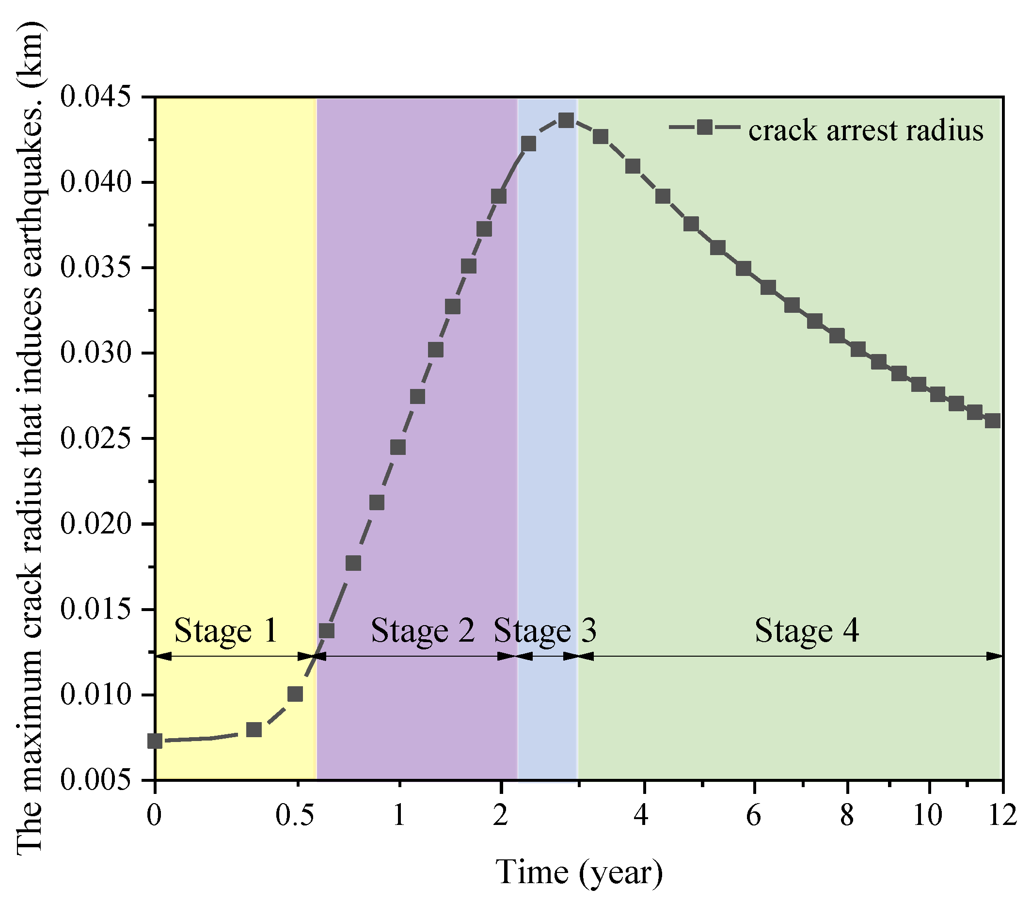
As illustrated in Figure 2, the evolution of the injection-induced seismic arrest radius undergoes four distinct phases: (1) Initial injection stage: The arrest radius gradually increases as fluid diffusion in the reservoir produces minimal stress perturbation on the fault. (2) Stable injection stage: The arrest radius exhibits rapid growth when the fluid reaches the fault core, accompanied by increasing effective stress in the fault core. (3) Injection termination stage: The arrest radius peaks when injection suddenly ceases, marking the maximum area of fault instability response. (4) Post-injection self-equilibration stage: The arrest radius progressively decreases as the fault system gradually attains a new stress equilibrium state.

Figure 2. Evolution of maximum seismic rupture radius induced by fluid injection.

4.2. Injecting Fluids Induces Seismic Magnitude Evolution

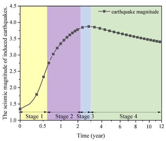
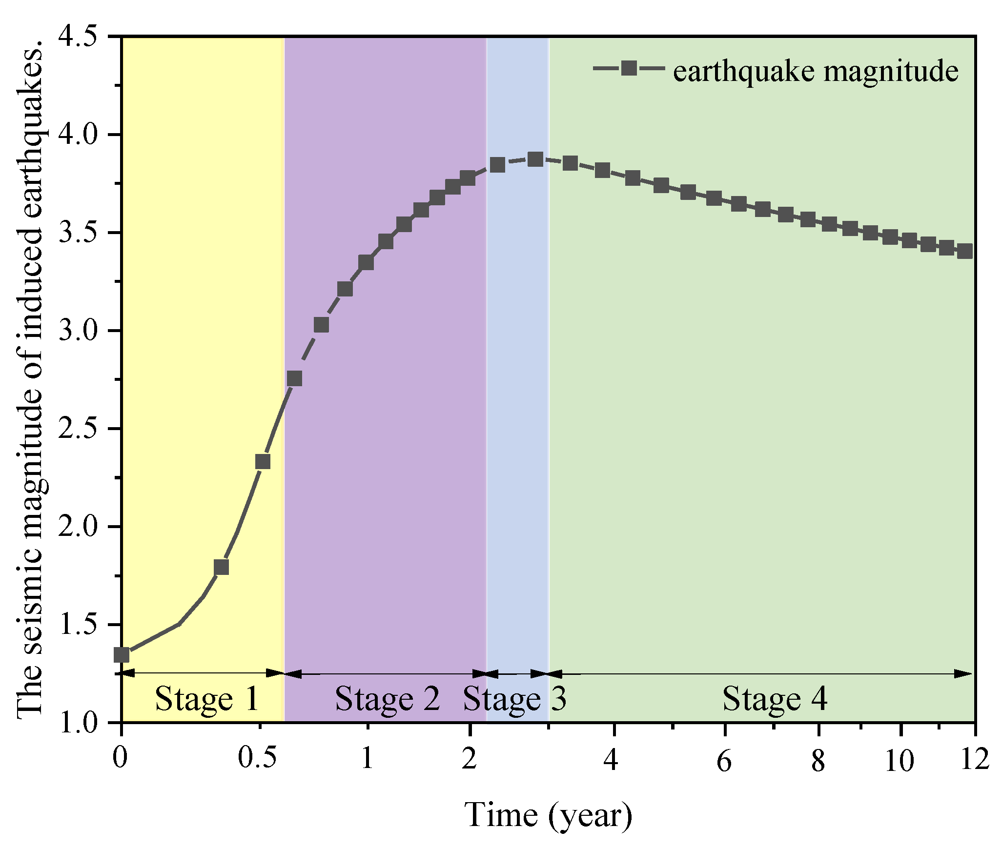
The magnitude of injection-induced seismicity is primarily governed by the competition between the in situ tectonic stress and the injection-induced stress perturbation on the fault. As shown in Figure 3, the seismic magnitude increases rapidly with growing arrest radius during the initial injection phase (Stage 1), where the injection-induced stress perturbation dominates the fault response. During the stable injection phase (Stage 2), the seismic magnitude continues to rise with increasing arrest radius, but at a progressively declining rate. This deceleration occurs because the stress perturbation effect at the rupture front gradually diminishes as the arrest radius expands, while the influence of tectonic stress becomes more pronounced, partially restraining seismic energy accumulation. The system reaches its peak hazard state in Stage 3 (injection termination), when both the arrest radius and seismic magnitude attain their maximum values. In the subsequent self-equilibration phase (Stage 4), the arrest radius and seismic magnitude gradually decline until a new equilibrium is established.

Figure 3. Evolution of seismic moment induced by fluid injection.

4.3. Factors Affecting the Radius and Magnitude of Induced Earthquake Induced Crack Arrest

This section aims to investigate the evolution of fault arrest radius and seismic magnitude assessment throughout the entire fluid injection process under various conditions, including different injection methods, fault types, fault-related locations, and injection well positions. By examining the variation trends of injection-induced fault arrest radius and predicting the occurrence timing of maximum seismic magnitude, this study provides operational safety recommendations for fluid injection practices in oilfields.

4.3.1. Different Types of Faults

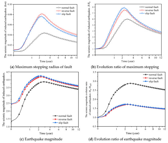
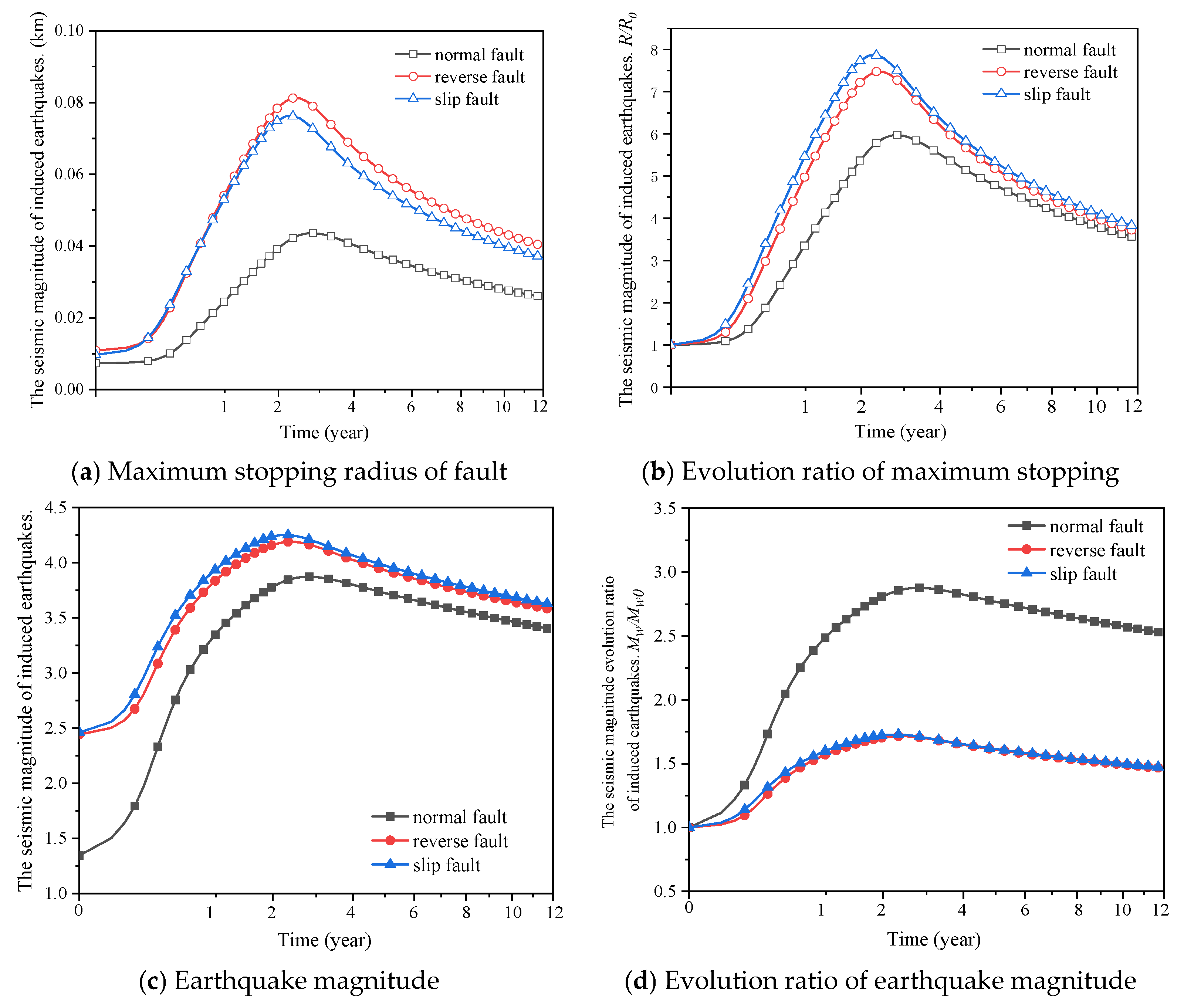
Under identical distances between injection wells and faults, we examine three fault types with distinct stress states (normal, reverse, and strike-slip faults) to investigate the maximum arrest radius (R) and induced seismic magnitude (M_w) resulting from injection-induced fault instability.

The distinct initial tectonic stress conditions under different fault stress regimes result in varying baseline values of fault arrest radius and seismic magnitude prior to fluid injection. Accordingly, this section presents comparative analyses of both absolute evolution values (R and M_w) and normalized evolution ratios (R/R₀ and M_w/M_w0) across the three fault stress regimes.

As illustrated in Figure 4a, reverse faults exhibit the largest absolute arrest radius (R) following well shutdown. However, Figure 4b demonstrates that strike-slip faults show the most significant normalized arrest radius evolution ratio (R/R₀), indicating they exhibit the strongest response to fluid injection, followed by reverse faults in terms of arrest radius development. Normal fault regimes display both the smallest absolute arrest radius (R) and normalized ratio (R/R₀), representing the least responsive stress state to fluid injection.

Figure 4. Analysis of maximum seismic rupture radius and seismic moment on faults under three different fault regimes.

Notably, when comparing induced seismic magnitudes across fault types (Figure 4c), strike-slip faults generate the highest absolute magnitude (M_w) post-shutdown. Conversely, Figure 4d reveals that normal faults produce the greatest normalized magnitude evolution ratio (M_w/M_w0). This suggests that while normal faults show limited geometrical response to injection (as reflected in arrest radius metrics), their stress state actually facilitates more intense seismic energy release relative to baseline conditions when subjected to fluid injection.

4.3.2. Relationship Between Fault and Injection Well Location

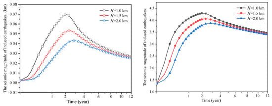
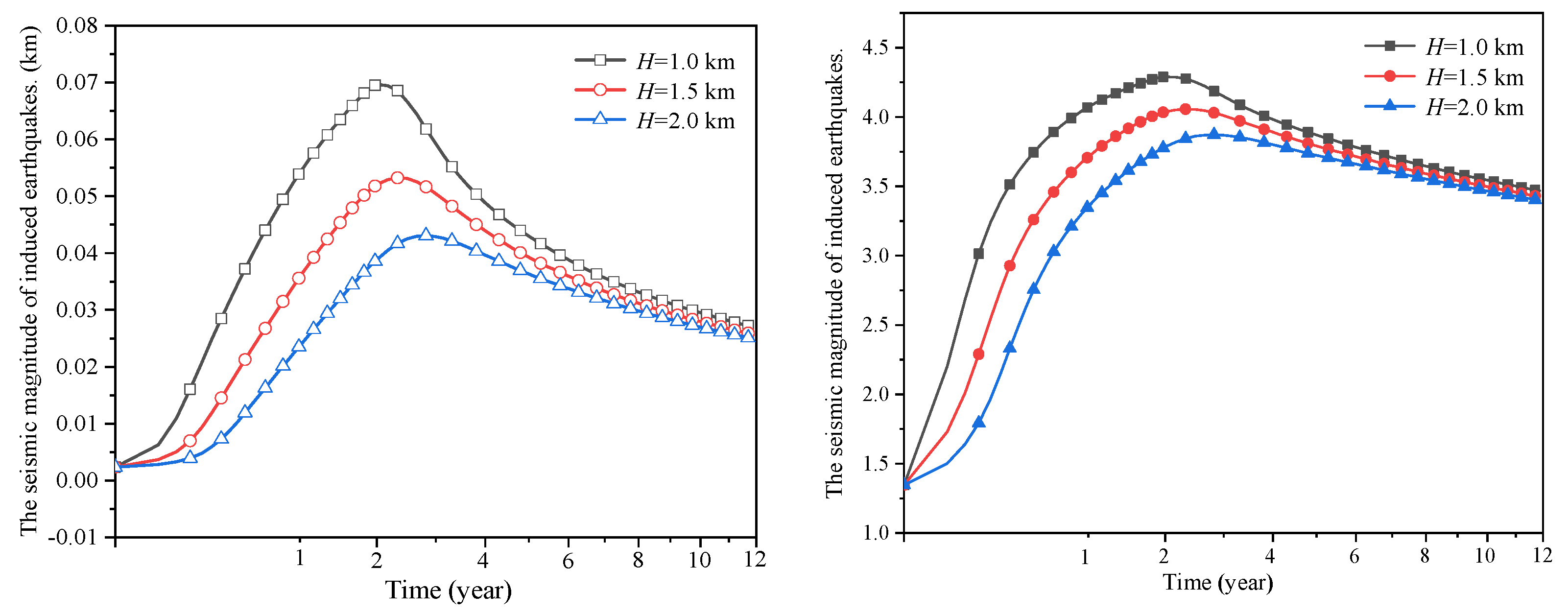
The evolution of fracture instability and stopping radius induced by fluid injection on the fault and earthquake magnitude at different distances of injection wells relative to the fault: 1.0 km, 1.5 km, and 2.0 km. Under three different distances, the evolution trend of the stopping radius and earthquake magnitude on the fault with fluid injection is roughly the same. As the stopping radius of the fault increases, the unstable rupture effect induced by injection on the edge of the fault rupture zone gradually decreases. Conversely, the original structural stress effect at the same location of the fault gradually increases, suppressing further seismic rupture at the edge of the fault rupture. As shown in Figure 5, the closer the distance between the fault and the injection well, the more significant the evolution of the fracture radius and earthquake magnitude on the fault. In addition, when injection suddenly stops, the closer the fault is to the injection well, the earlier the stopping radius and earthquake magnitude reach their maximum values. Therefore, faults closer to the injection well have a more pronounced response to fluid injection and reach the maximum values of fracture radius and earthquake magnitude earlier after sudden injection stops.

Figure 5. Analysis of maximum seismic rupture radius and seismic moment on faults under three different injection-well sites.

In summary, the conclusion drawn can be consistent with the analysis of the evolution of critical stiffness of faults under different injection well positions in the previous chapter: the evolution of critical stiffness of faults closer to the injection well is more significant, and the maximum critical stiffness of the fault after well closure is also greater, indicating that the closer the injection well is to the fault, the more likely it is to trigger an earthquake. The closer the distance between the injection well and the fault, the larger the stopping radius, the larger the range of unstable rupture, and the greater the earthquake magnitude.

4.3.3. Different Reservoir Permeability

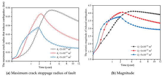
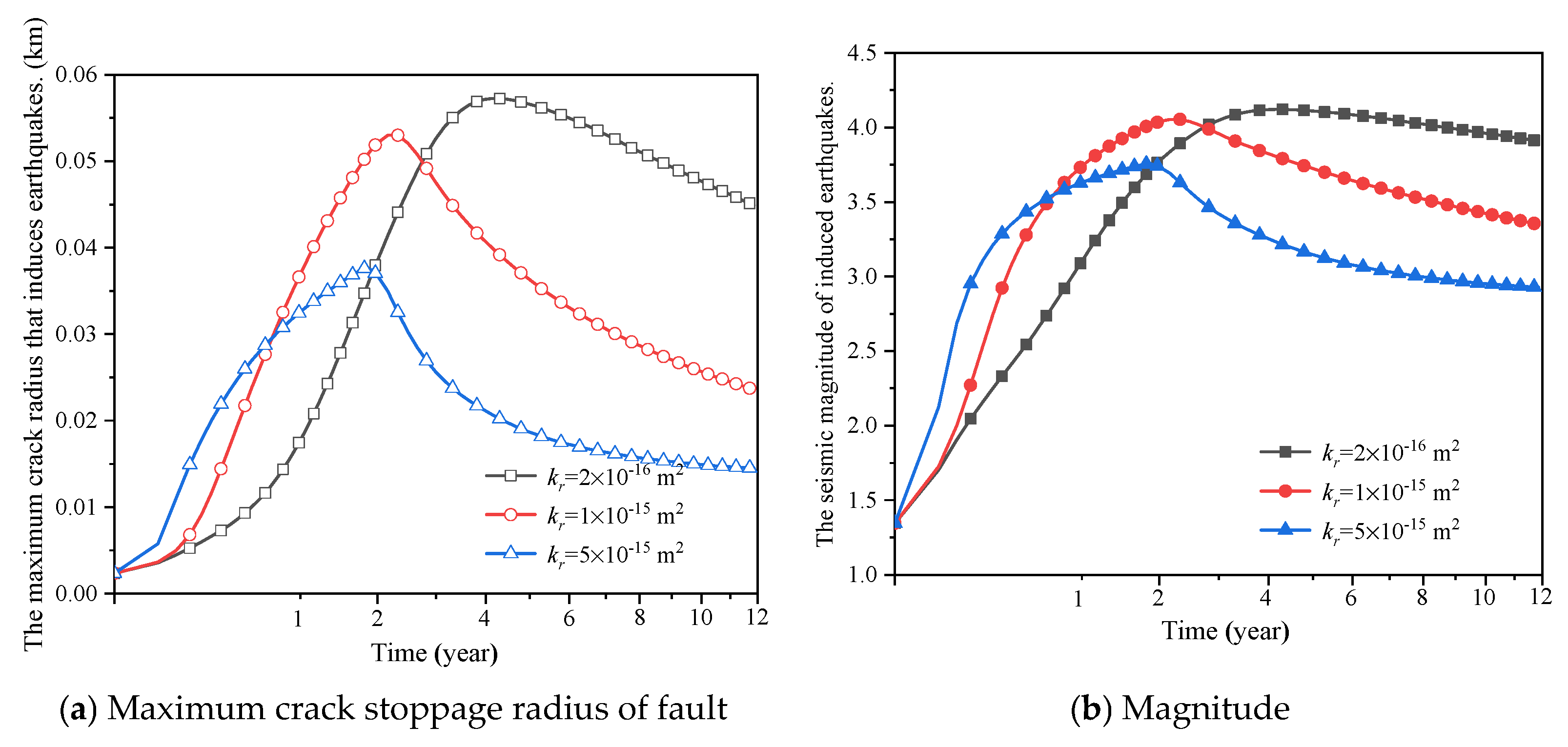
Injecting fluids into reservoirs with different permeabilities can trigger varying degrees of seismic response in faults. As shown in Figure 6, different permeability reservoirs were set up to study the evolution of fracture instability and stopping radius induced by fluid injection in faults, as well as the seismic magnitude. Figure 6 shows that compared to high permeability reservoir conditions, the evolution of the fracture stopping radius on faults under low permeability reservoir conditions has a shorter response time to fluid injection. Faults with low-permeability reservoirs have a relatively rapid increase in fracture radius during the early stage of fluid injection, and the time to reach the maximum fracture radius is also the fastest. This is due to the pore elasticity effect of rock mass, and the diffusion process of fluid in low-permeability reservoirs (before the fluid reaches the fault) will cause stress disturbance to the fault. In the initial stage of fluid injection, under reservoir conditions with high permeability, the stopping radius of the fault increases faster. When the injection suddenly stops, the maximum stopping radius of the fault under low-permeability reservoir conditions is greater. Similarly, reservoirs with lower permeability have a slower response to fluid injection compared to reservoirs with higher permeability, but they reach a larger seismic magnitude after injection stops. Therefore, at a constant injection rate, the lower the permeability of the reservoir, the larger the stopping radius and seismic magnitude on the fault. This conclusion can be consistent with the conclusion obtained in the previous chapter that the critical stiffness of faults is greater under low-permeability reservoir conditions after injection is stopped, proving that the possibility of triggering earthquakes and generating larger magnitudes under low-permeability reservoir conditions is greater.

Figure 6. Analysis of maximum seismic rupture radius and seismic moment on faults under different reservoir permeability.

4.4. Results and Engineering Validation of Induced Seismic Activity Model

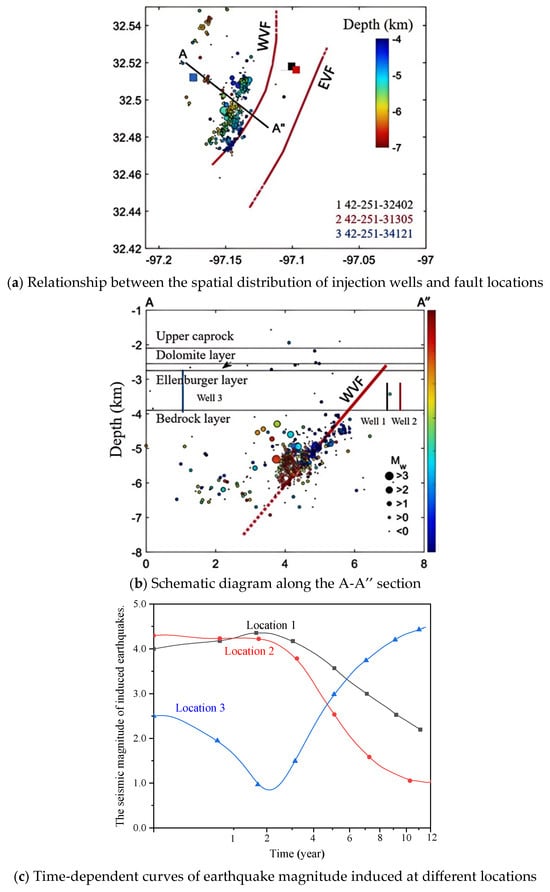
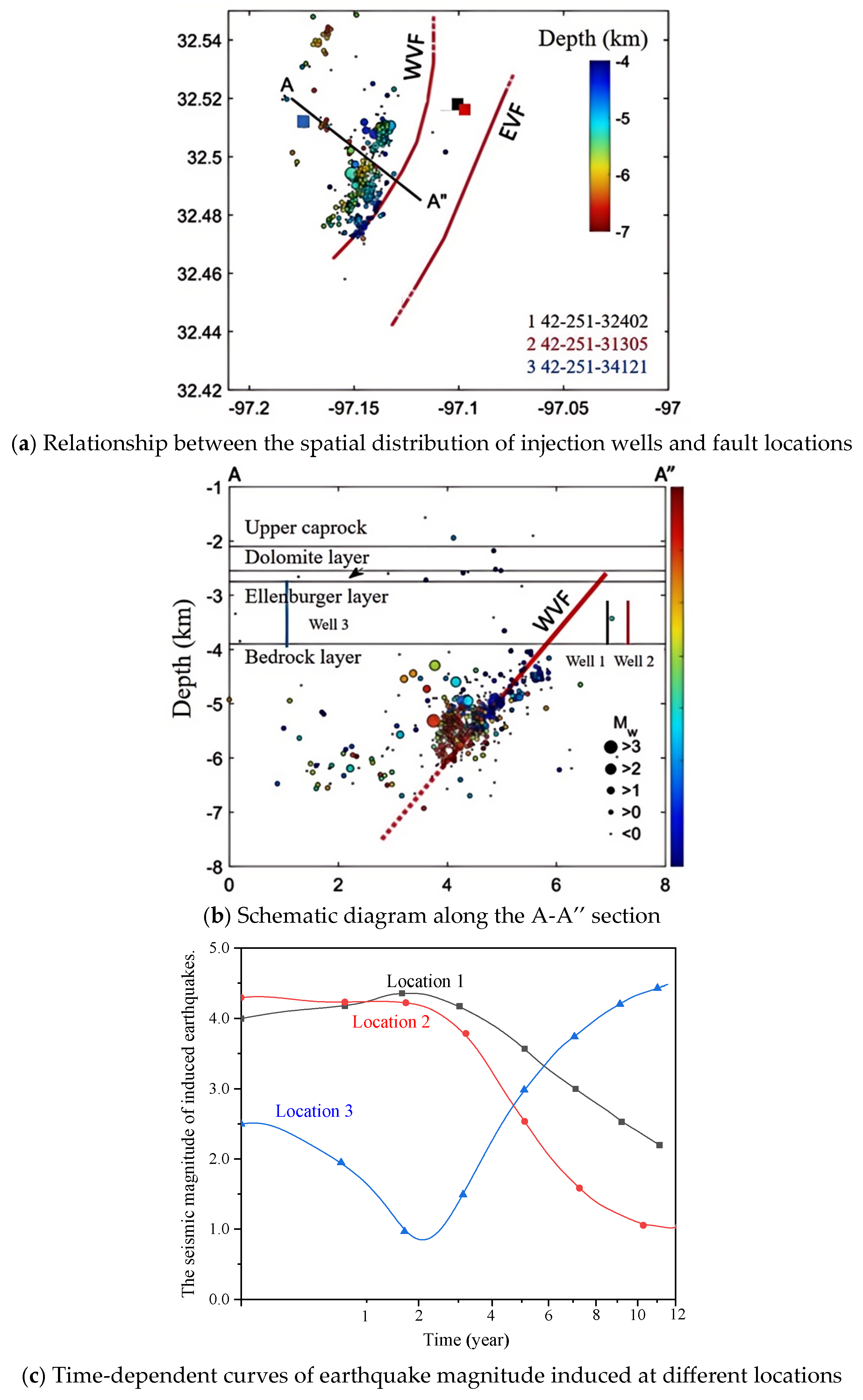
Figure 7 summarizes the spatiotemporal distribution characteristics of seismic data along faults in the Bend Arch Fort Worth Basin near Venus in northeastern Johnson County, Texas [42,43]. The three color blocks represent three SWD injection wells in Figure 7a, and Figure 7b shows a cross-sectional stratigraphic plan along A-A”, including the projected SWD wells and source locations (Figure 7a). As shown in Figure 7b, the small vertical lines in black, red and blue in the reservoir represent SWD injection wells. and the partial injection rates of the three injection wells can be seen in Figure 1b. To simplify the modeling process, three SWD injection wells were numbered and their injection rates were simplified as Q_SWD1 = 10 cubic meters per month, Q_SWD2 = 10 cubic meters per month, and Q_SWD3 = 5 cubic meters per month. The spatiotemporal distribution of seismic events detected around the bedrock layer and fault layer is represented by solid circles. The size of the circle represents the magnitude of the monitored earthquake, and the color of the circle represents the time of occurrence of the seismic event.

Figure 7. Location map of earthquakes and faults near Venus, TX.

Figure 7a shows the spatiotemporal distribution of a large number of earthquake events related to faults detected on site (filled circles of different sizes and colors). Earthquakes occur first in the upper part of the fault in the bedrock layer. As shown in Figure 7, the maximum magnitude occurs in the middle of the fault and in the later stage of fluid injection. In addition, the magnitude of earthquakes that occur in the central region is generally higher. Figure 7c shows the seismic magnitude analysis at different locations of faults in the bedrock layer of the numerical simulation. As shown in Figure 7c, it can be concluded that in the initial stage of fluid injection, the upper part of the bedrock fault layer will experience earthquakes first, but the magnitude will gradually decrease with injection time. On the contrary, in the initial stage of fluid injection, the seismic magnitude of the lower part of the basement fault layer is smaller than that of the upper part, but it gradually increases with fluid injection. This explains the on-site inspection results well: the upper part of the fault will first experience instability and rupture when fluid is first injected, but as the fluid injection time prolongs, the earthquake magnitude in the lower part of the fault will gradually increase, forming a more obvious earthquake delay phenomenon.

4.5. Analysis of Model Limitations and Outlook

The model compares two typical injection schemes (linear-rate injection and periodic injection) but does not cover complex field conditions such as variable flow rates, variable pressures, and intermittent or irregular injection. Furthermore, the model overlooks the impact of variations in the physical properties of the injected fluids. In actual engineering applications, fluids with differing viscosities, salinity levels and temperatures exhibit significant variations in seepage diffusion rates and pore pressure transmission efficiency; however, the model treats fluid properties uniformly and does not perform a differentiated analysis. Furthermore, the model does not account for engineering interference factors such as wellbore dimensions, minor deviations in injection depth, and formation leakage. It is suitable for medium- to long-term, routine, continuous, or periodic fluid injection projects, capable of accurately capturing the complete seismic evolution patterns during the initial injection phase, the stable injection phase, the sudden cessation phase, and the formation self-equilibrium phase, thereby effectively predicting the risk of delayed induced earthquakes following cessation of injection.

Future research could incorporate algorithms for the spatial random distribution of formation heterogeneity and anisotropy parameters. Furthermore, a fully coupled multi-field numerical model integrating flow, stress, temperature and chemistry could be developed, taking into account key influencing factors such as rock-water interaction, formation temperature evolution and differences in fluid properties, thereby enabling a comprehensive, full-cycle risk assessment of fluid injection-induced earthquakes.

5. Conclusions

In this section of the study, a calculation method was proposed to predict the maximum damage area and earthquake magnitude of faults induced by fluid injection, in order to accurately quantify the relationship between stress disturbance on the fault layer and induced seismic activity during the fluid injection process. In the proposed prediction method, the maximum damage area of the fault and the magnitude of the earthquake are positively correlated with the changes in effective forces on the fault, and negatively correlated with the background tectonic stress. By analyzing the stress field changes on the fault layer during the injection process of the established three-dimensional geological model, considering the evolution of fault permeability, the area where earthquake rupture occurs on the fault layer in fluid injection engineering is defined. The maximum damage area and earthquake magnitude induced by injection are calculated, and the proposed method for calculating the maximum earthquake magnitude induced by injection is verified using field data. The following conclusions are drawn from the study.

(1) In deep injection engineering, as the fluid continues to be injected, the effective force on the fault gradually decreases due to the transmission of pore elastic force, and the seismic rupture area on the fault will also increase accordingly. After the injection suddenly stops, the earthquake rupture area on the fault and the maximum induced earthquake magnitude reach their maximum values. Therefore, the maximum fluid injection-induced seismic event is more likely to occur after the fluid injection stops, and the delay effect of this injection-induced earthquake is consistent with the results obtained from the analysis and derivation of the modified fault critical stiffness evolution in the previous section.

(2) At the beginning of fluid injection, the stress disturbance caused by injection on the fault gradually increases the seismic rupture area on the fault, and the induced earthquake magnitude rapidly increases with the increase in the fault stopping radius. During the stage of stable fluid injection, the seismic magnitude continues to increase with the increase in the stopping radius on the fault. However, due to the decreasing stress disturbance effect at the tip of the fracture extension on the fault, the original structural stress on the fault gradually increases, and the rate of seismic magnitude growth gradually decreases with the injection time. After the injection of fluid suddenly stops, the stop radius and seismic magnitude along the fault will reach their maximum values; this is the stage of the injection project when earthquakes are most likely to occur. During the self-equilibrium stage of the entire geological body after injection stops, the maximum fracture radius and earthquake magnitude on the fault gradually decrease and return to a stable value.

(3) The periodic fluid injection scheme results in the largest area of fracture instability on the fault, while the linear growth injection scheme leads to the highest magnitude of injection-induced earthquakes. Under the stress state of strike-slip faults, the area of rupture and instability on the fault increases most significantly, while under the stress state of normal faults, the evolution of earthquake magnitude is more severe. Reservoirs with lower permeability, closer to the injection well, and the option of directly closing the injection well can result in the largest range of instability and rupture on the fault, as well as the highest seismic magnitude. Linear gradual closure of the well is the safest option.

References

- Yehya, A.; Basbous, J.; Maalouf, E. Analysis of the Hydrogeological Conditions Affecting Fault Response to Nearby Hydraulic Fracturing. J. Geophys. Res. Solid Earth 2022, 127, e2022JB024881. [Google Scholar] [CrossRef] [Scilit]
- Zhang, N.; Zhou, L.; Li, Z. Typical characteristics and research progress of fluid injection-induced seismic activity. Prog. Geophys. Sci. 2024, 39, 2188–2206. [Google Scholar]
- Alghannam, M.; Juanes, R. Understanding rate effects in injection-induced earthquakes. Nat. Commun. 2020, 11, 3053. [Google Scholar] [CrossRef] [Scilit] [PubMed]
- Healy, J.H.; Rubey, W.W.; Griggs, D.T.; Raleigh, C.B. The Denver Earthquakes. Science 1968, 161, 1301–1310. [Google Scholar] [CrossRef] [Scilit]
- Wang, Z.; Wang, X.; Ma, S.; Lei, X.; Liu, P. Spatiotemporal distribution characteristics of water-induced earthquakes in Rongchang area, Chongqing. J. Seismol. Geol. 2018, 40, 523–538. [Google Scholar]
- Benson, P.M.; Austria, D.C.; Gehne, S.; Butcher, E.; Harnett, C.E.; Fazio, M.; Rowley, P.; Tomas, R. Laboratory simulations of fluid-induced seismicity, hydraulic fracture, and fluid flow. Geomech. Energy Environ. 2020, 24, 100169. [Google Scholar] [CrossRef] [Scilit]
- Davies, R.; Foulger, G.; Bindley, A.; Styles, P. Induced seismicity and hydraulic fracturing for the recovery of hydrocarbons. Mar. Pet. Geol. 2013, 45, 171–185. [Google Scholar] [CrossRef] [Scilit]
- Frohlich, C. Two-year survey comparing earthquake activity and injection-well locations in the Barnett Shale. Proc. Natl. Acad. Sci. USA 2012, 109, 13934–13938. [Google Scholar] [CrossRef] [Scilit]
- Cappa, F.; Rutqvist, J.; Yamamoto, K. Modeling crustal deformation and rupture processes related to upwelling of deep CO2-rich fluids during the 1965–1967 Matsushiro earthquake swarm in Japan. J. Geophys. Res. Solid Earth 2009, 114, B10. [Google Scholar] [CrossRef] [Scilit]
- Keranen, K.M.; Weingarten, M.; Abers, G.A.; Bekins, B.A.; Ge, S. Sharp increase in central Oklahoma seismicity since 2008 induced by massive wastewater injection. Science 2014, 345, 448–451. [Google Scholar] [CrossRef] [Scilit]
- Di Luccio, F.; Chiodini, G.; Caliro, S.; Cardellini, C.; Convertito, V.; Pino, N.A.; Tolomei, C.; Ventura, G. Seismic signature of active intrusions in mountain chains. Sci. Adv. 2018, 4, e1701825. [Google Scholar] [CrossRef] [Scilit] [PubMed]
- Zoback, M.D.; Gorelick, S.M. Earthquake triggering and large-scale geologic storage of carbon dioxide. Proc. Natl. Acad. Sci. USA 2012, 109, 10164–10168. [Google Scholar] [CrossRef] [Scilit]
- Duan, W.; Zhu, Z.; Liu, J.; Zhuang, R.; Li, S. Analysis of seismic activity before and after water storage in Ludila Reservoir, Jinsha River. J. Disaster Prev. Mitig. 2023, 39, 48–55. [Google Scholar]
- Pacala, S.; Socolow, R. Stabilization wedges: Solving the climate problem for the next 50 years with current technologies. Science 2004, 305, 968–972. [Google Scholar] [CrossRef] [Scilit]
- Vidal-Gilbert, S.; Tenthorey, E.; Dewhurst, D.; Ennis-King, J.; Van Ruth, P.; Hillis, R. Geomechanical analysis of the Naylor Field, Otway Basin, Australia: Implications for CO2 injection and storage. Int. J. Greenh. Gas Control 2010, 4, 827–839. [Google Scholar] [CrossRef] [Scilit]
- Yu, H.; Zhang, G.; Yan, X. Research Progress on the Mechanism of CO2 Sequestration Inducing Near-Fault Activation. J. Huaqiao Univ. (Nat. Sci. Ed.) 2024, 45, 136–149. [Google Scholar]
- Chen, Q.; Zhang, X.; Zhao, C. Advances in Research on Hydraulic Fracturing-Induced Earthquakes. Seismology 2023, 43, 215–227. [Google Scholar]
- Chen, Q.; Liu, Y.; Jin, X.; Lin, R.; Pan, Y.; Xie, J. Information Acquisition Methods for Granite-type Hot Dry Rock Reservoirs and Controlled Fracturing Technology. Drill. Eng. 2023, 50, 50–55. [Google Scholar]
- Ellsworth, W.L. Injection-induced earthquakes. Science 2013, 341, 1225942. [Google Scholar] [CrossRef] [Scilit]
- King Hubbert, M.; Rubey, W.W. Role of fluid pressure in mechanics of overthrust faulting: I. Mechanics of fluid-filled porous solids and its application to overthrust faulting. Geol. Soc. Am. Bull. 1959, 70, 115–166. [Google Scholar] [CrossRef] [Scilit]
- Eyre, T.S.; Eaton, D.W.; Garagash, D.I.; Zecevic, M.; Venieri, M.; Weir, R.; Lawton, D. The role of aseismic slip in hydraulic fracturing-induced seismicity. Sci. Adv. 2019, 5, eaav7172. [Google Scholar] [CrossRef] [Scilit]
- Galloway, E.; Hauck, T.; Corlett, H.; Pena, D.; Schultz, R. Faults and associated karst collapse suggest conduits for fluid flow that influence hydraulic fracturing-induced seismicity. Proc. Natl. Acad. Sci. USA 2018, 115, E10003–E10012. [Google Scholar] [CrossRef] [Scilit]
- Byrne, H.; Silva, J.A.; Plesch, A.; Juanes, R.; Shaw, J.H. The Groundbreaking Experiment in Earthquake Control at Rangely, Colorado, Revisited. Geophys. Res. Lett. 2020, 47, e2020GL088257. [Google Scholar] [CrossRef] [Scilit]
- Majid, K.; He, X.Q.; Song, D.Z.; Tian, X.H.; Li, Z.L.; Xue, Y.R.; Khurram, S.A. Extracting and predicting rock mechanical behavior based on microseismic spatio-temporal response in an ultra-thick coal seam mine. Rock Mech. Rock Eng. 2023, 56, 3725–3754. [Google Scholar]
- Zhu, S.; Cao, J.; Feng, C.; Wang, J.; Meng, J.; Qi, B. Study on the risk of fault instability induced by water reinjection in deep thermal reservoirs with low protrusions in Gaoyang, Hebei Province. Acta Geomech. Sin. 2023, 29, 220–235. [Google Scholar]
- Schultz, R.; Wang, R.J.; Gu, Y.J.; Haug, K.; Atkinson, G. A seismological overview of the induced earthquakes in the Duvernay play near Fox Creek, Alberta. J. Geophys. Res. Solid Earth 2017, 122, 492–505. [Google Scholar] [CrossRef] [Scilit]
- Patricia, M.G.; Marco, B.; Grzegorz, K.; Georg, D. Stress tensor changes related to fluid injection at The Geysers geothermal field, California. Geophys. Res. Lett. 2013, 40, 2596–2601. [Google Scholar] [CrossRef] [Scilit]
- Goebel, T.H.W.; Brodsky, E.E. The spatial footprint of injection wells in a global compilation of induced earthquake sequences. Science 2018, 361, 899–904. [Google Scholar] [CrossRef] [Scilit]
- Zhang, X.; Sanderson, D.J. Numerical modelling of the effects of fault slip on fluid flow around extensional faults. J. Struct. Geol. 1996, 18, 109–119. [Google Scholar] [CrossRef] [Scilit]
- Zhu, A.; Sun, Z.; Jiang, C.; Chen, S.; Zhang, D.; Cui, G. Numerical simulation of fault dynamic response under different water injection methods. J. Seismol. 2021, 43, 730–744. [Google Scholar]
- Sun, Z.H.; Elsworth, D.; Cui, G.L.; Li, Y.C.; Zhu, A.Y.; Chen, T.Y. Impacts of Rate of Change in Effective Stress and Inertial Effects on Fault Slip Behavior: New Insights Into Injection-Induced Earthquakes. J. Geophys. Res. Solid Earth 2024, 129, e2023JB027126. [Google Scholar] [CrossRef] [Scilit]
- Huang, Y.; Ma, S.; Li, X. Research Progress on Water Injection-Induced Earthquakes. J. Seism. Eng. 2023, 45, 387–400. [Google Scholar]
- He, D.F.; Lu, R.Q.; Huang, H.Y.; Wang, X.S.; Jiang, H.; Zhang, W.K. Tectonic and geological setting of the earthquake hazards in the Changning shale gas development zone, Sichuan Basin, SW China. Pet. Explor. Dev. 2019, 46, 1051–1064. [Google Scholar] [CrossRef] [Scilit]
- Gan, Q.; Elsworth, D. Analysis of fluid injection-induced fault reactivation and seismic slip in geothermal reservoirs. J. Geophys. Res. Solid Earth 2014, 119, 3340–3353. [Google Scholar] [CrossRef] [Scilit]
- Elsworth, D.; Spiers, C.J.; Niemeijer, A.R. Understanding induced seismicity. Science 2016, 354, 1380–1381. [Google Scholar] [CrossRef] [Scilit]
- Galis, M.; Ampuero, J.P.; Mai, P.M.; Cappa, F. Induced seismicity provides insight into why earthquake ruptures stop. Sci. Adv. 2017, 3, eaap7528. [Google Scholar] [CrossRef] [Scilit]
- Norbeck, J.H.; Horne, R.N. Maximum magnitude of injection-induced earthquakes: A criterion to assess the influence of pressure migration along faults. Tectonophysics 2018, 733, 108–118. [Google Scholar] [CrossRef] [Scilit]
- Bommer, J.J.; Verdon, J.P. The maximum magnitude of natural and induced earthquakes. Geomech. Geophys. Geo-Energy Geo-Resour. 2024, 10, 172. [Google Scholar] [CrossRef] [Scilit]
- Brown, M.R.M.; Ge, S. Small earthquakes matter in injection-induced seismicity. Geophys. Res. Lett. 2018, 45, 5445–5453. [Google Scholar] [CrossRef] [Scilit]
- Scales, M.M.; DeShon, H.R.; Magnani, M.B.; Walter, J.I.; Quinones, L.; Pratt, T.L.; Hornbach, M.J. A Decade of Induced Slip on the Causative Fault of the 2015 Mw 4.0 Venus Earthquake, Northeast Johnson County, Texas. J. Geophys. Res. Solid Earth 2017, 122, 7879–7894. [Google Scholar] [CrossRef] [Scilit]
- Hennings, P.H.; Snee, J.E.L.; Osmond, J.L.; DeShon, H.R.; Dommisse, R.; Horne, E.; Lemons, C.; Zoback, M.D. Injection-Induced Seismicity and Fault-Slip Potential in the Fort Worth Basin, Texas. Bull. Seismol. Soc. Am. 2019, 109, 1615–1634. [Google Scholar] [CrossRef] [Scilit]
- Chang, K.W.; Yoon, H. Permeability-controlled migration of induced seismicity to deeper depths near Venus in North Texas. Sci. Rep. 2022, 12, 1382. [Google Scholar]
- Chang, K.W.; Yoon, H. Hydro-mechanical controls on the spatio-temporal patterns of injection-induced seismicity in different fault architecture: Implication for 2013–2014 Azle earthquakes. J. Geophys. Res. Solid Earth 2020, 125, e2020JB020402. [Google Scholar] [CrossRef] [Scilit]
- Chen, R.; Xue, X.; Yao, C.; Datta-Gupta, A.; King, M.J.; Hennings, P.; Dommisse, R. Coupled Fluid Flow and Geomechanical Modeling of Seismicity in the Azle Area North Texas. SPE Reserv. Eval. Eng. 2020, 23, 1006–1018. [Google Scholar] [CrossRef] [Scilit]
Disclaimer/Publisher’s Note: The statements, opinions and data contained in all publications are solely those of the individual author(s) and contributor(s) and not of MDPI and/or the editor(s). MDPI and/or the editor(s) disclaim responsibility for any injury to people or property resulting from any ideas, methods, instructions or products referred to in the content. |
© 2026 by the authors. Licensee MDPI, Basel, Switzerland. This article is an open access article distributed under the terms and conditions of the Creative Commons Attribution (CC BY) license.