SABI: Self-Adaptive Bias for Imbalanced Data Classification

Abstract

Class imbalance remains a significant challenge in classification, often leading to poor generalization on underrepresented classes. While Oversampling methods mitigate this issue by replicating minority class instances to balance class distributions, they typically overlook the informativeness of individual samples. In this paper, we propose an entropy-guided data selection strategy that dynamically prioritizes samples exhibiting frequent prediction changes during training, that is, those with high predictive entropy. Such uncertain samples are expected to contribute more effectively to the learning process. Moreover, we incorporate a credal set-based weighting scheme that adjusts class-wise selection probabilities according to global imbalance severity, quantified using the Gini coefficient. This adjustment penalizes overrepresented classes while increasing the sampling probability of rare but uncertain examples. Experiments on benchmark datasets show that the proposed method improves overall classification performance across imbalanced data settings, while also showing a more balanced trade-off across head, body, and tail classes.

1. Introduction

Imbalanced class distributions not only degrade performance on minority classes but also hinder robust generalization across the full class distribution. As a result, models trained on such data often become biased toward majority classes [1], leading to degraded performance on minority classes. Traditional Oversampling methods attempt to address this issue by replicating or synthetically augmenting minority-class samples to balance the training set [2]. However, these methods generally do not account for the informativeness or uncertainty of individual samples, and may repeatedly select less informative instances. By contrast, uncertainty-based selection has been widely explored in active learning, where samples with uncertain predictions are often regarded as more informative for improving the model [3].

This paper proposes SABI, a data selection-based approach that directly targets informative samples rather than merely equalizing class distributions. We assume that samples whose predicted labels frequently change during training, that is, those with high uncertainty, contribute more to the model’s learning and should therefore be sampled more frequently. To operationalize this idea, we compute the predictive entropy of each sample over training epochs and use this as a proxy for model uncertainty. Higher-entropy samples, which indicate fluctuating predictions, are prioritized during mini-batch construction.

To further integrate class imbalance into the sample selection process, we borrow from credal set theory and construct lower bounds for class probabilities based on the overall imbalance degree, which we quantify using the Gini coefficient [4]. Specifically, this formulation allows us to modulate the influence of sample uncertainty by penalizing overrepresented classes and amplifying the selection probability of underrepresented ones. The resulting method dynamically balances uncertainty-driven sampling with imbalance-aware weighting, without relying on synthetic data augmentation.

In SABI, credal set reasoning is used as a motivation for conservative class-level correction rather than as a full credal classification framework. The proposed formulation therefore combines the instance-level uncertainty used in SAB with an imbalance-aware prior derived from class frequencies. This distinguishes SABI from SAB by allowing the sampling probability to reflect both recent prediction instability and global class distribution.

Our main contributions are as follows:

• We formulate class-imbalanced data selection as a joint problem of instance-level uncertainty and class-level distributional bias, extending SAB to long-tailed classification settings.
• We introduce a Gini-adjusted credal set weighting term that extends SAB by allowing the sampling distribution to adapt to global class imbalance, thereby increasing the sampling probability of underrepresented classes while preserving uncertainty-based sample selection.
• We empirically show that SABI provides a more balanced trade-off between head, body, and tail classes than SAB and conventional Oversampling, especially under long-tail distributions.

The remainder of this paper is structured as follows. Section 2 reviews related work on imbalanced learning, uncertainty estimation, and credal set theory. Section 3 introduces our proposed method, detailing the entropy computation, Gini-adjusted credal set weighting, and sampling procedure. Section 4 describes the experimental setup, datasets, evaluation metrics, results, and ablation analyses. Finally, Section 5 concludes the paper and outlines directions for future research.

2. Related Works

2.1. Credal Set

The credal set framework models uncertainty using sets of probability distributions rather than single-point estimates, allowing for more robust reasoning under imprecision and data imbalance. Initially introduced by Walley [5], credal sets provide a conservative probabilistic representation by specifying lower and upper bounds for each class probability, thereby capturing epistemic uncertainty explicitly. In classification tasks, this framework enables the use of dominance-based or imprecise decision rules that can withhold decisions in cases of high ambiguity. In the context of imbalanced classification, credal sets have been applied to adjust prediction confidence by penalizing overrepresented classes and enhancing the representation of minority classes. Recent work [6] extends credal classification to deep neural networks, demonstrating that uncertainty-aware predictions can improve robustness under skewed data distributions. Building on this line of research, we incorporate a credal set-based adjustment into the sampling probability. Specifically, we modulate the selection weight for each data point using a lower bound on class probability derived from the class frequency and a global imbalance metric—Gini’s coefficient. This allows the sampling process to jointly reflect predictive uncertainty and structural dataset imbalance.

Compared to methods such as recency bias [7], which emphasize recent prediction volatility, or importance sampling [8], which prioritizes high-gradient data, our approach uses a class-distribution-aware correction inspired by credal set reasoning to guide data selection in an imbalance-sensitive manner. Unlike Oversampling techniques that introduce redundancy, our method adaptively selects high-uncertainty samples from underrepresented classes, leading to improved generalization without overfitting.

2.2. Data Sampling

Recent studies have shown that how mini-batches are configured affects performance when using deep neural networks (DNNs) for text or image classification. Accordingly, various methods have been proposed to determine which training samples should be selected based on the model’s learning behavior.

Traditionally, methods for classifying imbalanced data involve either oversampling the minority class [2] or undersampling the majority class [9,10,11]. Additionally, the SMOTE [2,12] method, which creates synthetic samples, is employed. If the above resampling methods are used without checking the distribution of the data, problems such as information loss and overfitting may appear.

In addition, there are known methods that calculate the loss value or uncertainty for each sample using the results generated during the learning process and utilizing them for sampling [13,14]. When using loss directly, there is an online batch selection [15] method that prioritizes learning data with high loss values to accelerate the convergence speed of the model. However, excessive emphasis on difficult samples may lead to overfitting. Also, in the case of learning data with small loss first, it is possible to learn strongly for noise data, but the learning speed may slow down significantly because the loss is small and the gradient is small [16].

Curriculum learning has also been proposed, where easy samples are introduced early in training and more difficult samples are presented later [17]. When uncertainty is used for sampling, the predicted probabilities of each sample are used to compute entropy, which serves as a measure of uncertainty. These uncertainty estimates are then used to construct mini-batches for training [7,18,19,20]. Prior studies have reported that using prediction information from the most recent stage of training can be more effective than using prediction information accumulated over the entire training process.

2.3. Classification

In the past, text classification problems have been addressed using statistical approaches such as Bag of Words and TF-IDF, and have continued to evolve with methods like CNN [21], LSTM, and transformers [22]. Recently, in line with this trend, classification experiments using large language models (LLMs) have been actively conducted [23,24]. These methods aim to generate predefined labels by utilizing prompt-based in-context learning of LLMs. While LLMs can achieve excellent performance in classification tasks, additional fine-tuning may be required to improve performance on datasets with limited conditions. Since LLMs have a large number of parameters, training takes a long time and consumes significant computational resources, which can be a limitation in general environments. To overcome these limitations, it may be necessary to use relatively smaller models. Smaller models offer practical advantages by reducing computational resources through fewer parameters and faster training times.

3. Proposed Method

We introduce SABI, an extension of SAB [20] for class-imbalanced classification. SAB selects training instances according to their recent prediction histories, but it does not explicitly account for the class distribution. This can be problematic in long-tailed settings, where majority classes provide more candidate instances and may still dominate the sampled mini-batches even under uncertainty-based sampling.

The goal of SABI is therefore not to replace SAB, but to extend its uncertainty-driven sampling behavior to long-tailed settings by incorporating a lightweight class-distribution-aware correction. This extension allows the sampling distribution to reflect global class imbalance while retaining the instance-level uncertainty estimation of SAB.

SABI addresses this issue by combining instance-level uncertainty with a class-level imbalance prior. The uncertainty term follows the SAB sampling scheme and captures how unstable or error-prone each instance is during training. The imbalance term, on the other hand, increases the sampling weight of instances from underrepresented classes. We use the Gini coefficient to control the relative contribution of these two terms. When the class distribution is close to uniform, SABI remains close to SAB. As the distribution becomes more skewed, the imbalance-aware term plays a larger role in the final sampling probability.

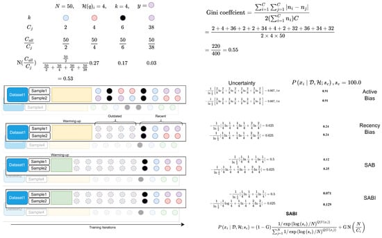
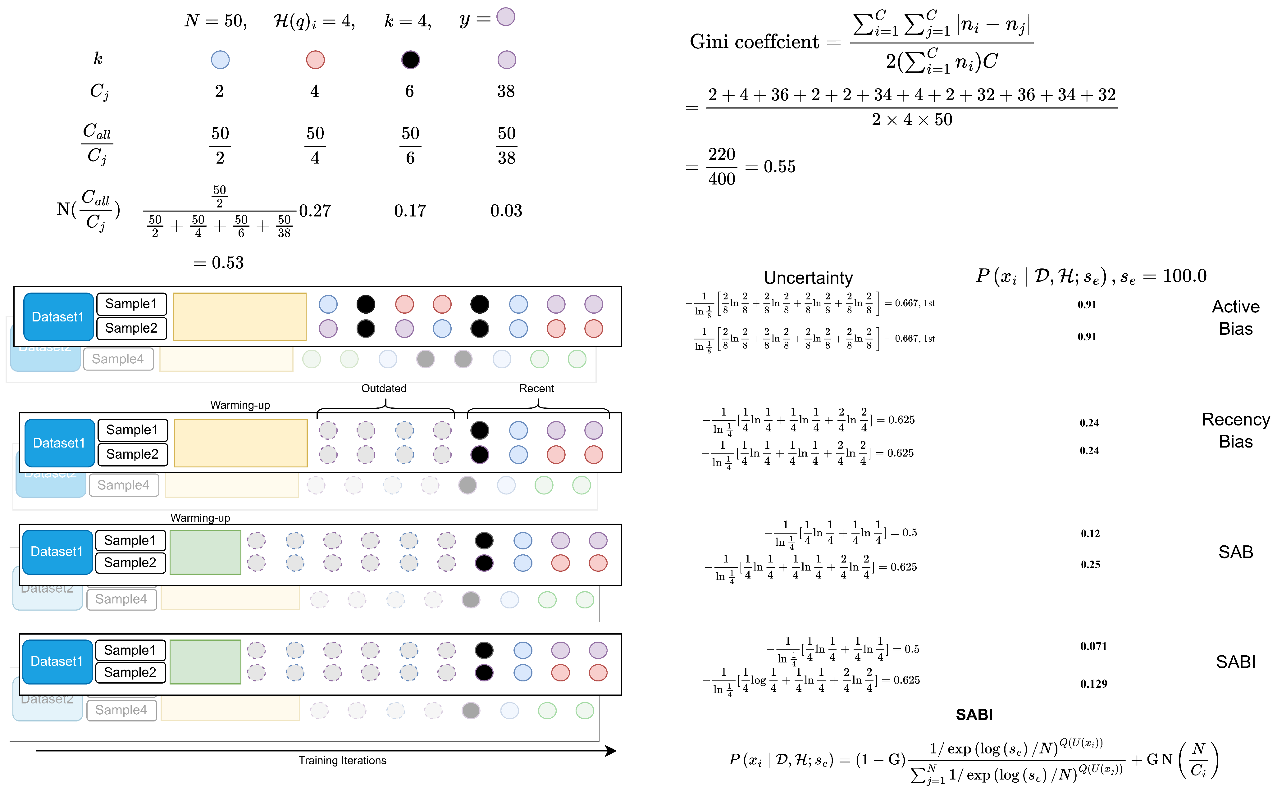
Figure 1 illustrates the overall framework of SABI. The proposed method computes uncertainty from recent prediction histories while excluding correctly predicted cases, adaptively determines the warming-up period according to the learning dynamics of each dataset, and adjusts the final sampling probability using class-distribution information.

Figure 1. Overall framework of SABI. SAB and SABI estimate sample uncertainty from recent prediction histories and use an adaptive warming-up period. SABI further incorporates a class-distribution-aware probability component into the final sampling probability, enabling the sampler to consider both instance-level uncertainty and class-level imbalance.

3.1. Problem Definition

In standard mini-batch training, model parameters are updated using a batch $\mathcal{B}$ sampled from the training set:

$${\theta }_{t+1}={\theta }_t-\eta \nabla \left({\displaystyle \frac{1}{\left|\mathcal{B}\right|}}\sum _{x_i\in \mathcal{B}}{f}_{x_i}\left({\theta }_t\right)\right),$$

(1)

where $\eta$ is the learning rate, ${\theta }_t$ denotes the model parameters at step t, and $f_{x_i}\left({\theta }_t\right)$ is the loss for instance $x_i$.

Uniform sampling treats all instances equally, regardless of how informative they are for the current model. Class-balanced sampling or oversampling can alleviate class imbalance, but it may repeatedly select minority-class instances without considering their learning value. SABI instead defines a sampling distribution that takes both predictive uncertainty and class imbalance into account.

Let $\mathcal{D}$ be the training dataset and $\mathcal{H}$ be the recent prediction history of training instances. SABI samples a mini-batch $\mathcal{U}$ from a distribution $P_{\mathrm{SABI}}\left(x_i\right)$:

$$\mathcal{U}\sim P_{\mathrm{SABI}}\left(x_i\right).$$

(2)

The update rule is then written as:

$${\theta }_{t+1}={\theta }_t-\eta \nabla \left({\displaystyle \frac{1}{\left|\mathcal{U}\right|}}\sum _{x_i\in \mathcal{U}}{f}_{x_i}\left({\theta }_t\right)\right).$$

(3)

This sampling scheme makes the mini-batch composition depend on both the model’s current learning state and the global class distribution.

3.2. SAB Backbone: Instance-Level Predictive Uncertainty

SABI uses the uncertainty estimation strategy of SAB as its instance-level sampling component. For each training instance, SAB keeps a recent history of predicted labels and estimates uncertainty from the inconsistency of those predictions. Intuitively, instances whose predicted labels fluctuate over training are more likely to be informative than instances that are already predicted consistently.

For each instance $x_i$, we maintain a label history ${\mathcal{H}}_i\left(q\right)$ with a sliding window of size q:

$${\mathcal{H}}_i\left(q\right)=\{{\widehat{y}}_{t_1},{\widehat{y}}_{t_2},\dots ,{\widehat{y}}_{t_q}\},$$

(4)

where ${\widehat{y}}_t=\Phi (x_i;{\theta }_t)$ is the predicted label of $x_i$ at step t, and $\Phi$ denotes the classification model.

Following SAB, we compute uncertainty from incorrect predictions in the recent history. This excludes cases where the model already predicts the correct label and places more emphasis on instances that remain misclassified or unstable. The empirical probability that $x_i$ is predicted as class j is defined as:

$$p(y_i=j\mid x_i)={\displaystyle \frac{{\sum }_{\widehat{y}\in {\mathcal{H}}_i\left(q\right)}\mathbb{1}(\widehat{y}=j\wedge \widehat{y}\ne y_i)}{|{\mathcal{H}}_i\left(q\right)|}},$$

(5)

where $y_i$ is the ground-truth label and $\mathbb{1}(·)$ is an indicator function.

The uncertainty score is computed using normalized entropy:

$$U\left(x_i\right)={\displaystyle \frac{1}{log\left(k\right)}}entropy\left(p(y_i\mid x_i)\right),$$

(6)

where k is the number of classes and

$$entropy\left(p(y_i\mid x_i)\right)=-{\displaystyle \sum _{j=1}^k}p(y_i=j\mid x_i)logp(y_i=j\mid x_i).$$

(7)

A higher value of $U\left(x_i\right)$ indicates that the instance has been predicted incorrectly or inconsistently in recent training steps. Such instances are assigned higher sampling priority in the uncertainty-based component.

Using this score, the SAB sampling probability is defined as:

$$P_{\mathrm{SAB}}\left(x_i\right)={\displaystyle \frac{1/exp{\left(log\left(s_e\right)/N\right)}^{Q\left(U\left(x_i\right)\right)}}{{\sum }_{l=1}^{N}1/exp{\left(log\left(s_e\right)/N\right)}^{Q\left(U\left(x_l\right)\right)}}},$$

(8)

where N is the number of training instances, $s_e$ is the selection pressure, and

$$Q\left(U\left(x_i\right)\right)=\lceil (1-U\left(x_i\right))N\rceil$$

(9)

denotes the quantized uncertainty rank.

In SABI, $P_{\mathrm{SAB}}\left(x_i\right)$ serves as the instance-level uncertainty term. The main difference from SAB is that SABI further adjusts this probability using the class distribution.

3.3. Adaptive Warming-Up Period

Prediction histories are unreliable at the very beginning of training. Therefore, the model is first trained for a warming-up period before uncertainty-based sampling is applied. A fixed warming-up period, however, may not be suitable for all datasets. Some datasets stabilize within a few epochs, whereas others require a longer period before the prediction history becomes meaningful.

SABI follows the adaptive warming-up strategy of SAB. In this work, the end of the warming-up period is determined using the validation loss. Let $L_n^{\mathrm{val}}$ denote the validation loss measured at the end of epoch n. Since the criterion compares two consecutive changes in validation loss, it is evaluated from $n\ge 2$. The adaptive warming-up epoch is defined as:

$$e_0=min\left\{n\ge 2:\left|L_n^{\mathrm{val}}-L_{n-1}^{\mathrm{val}}\right|<\left|L_{n-1}^{\mathrm{val}}-L_{n-2}^{\mathrm{val}}\right|\right\}.$$

(10)

This criterion ends the warming-up period when the magnitude of validation-loss improvement begins to decrease. The prediction history collected up to epoch $e_0$ is then used to set the sliding window and compute uncertainty scores. This allows the sampling process to start earlier for datasets that stabilize quickly, while still allowing a longer warm-up period for more difficult datasets.

3.4. Class Imbalance Estimation with the Gini Coefficient

Uncertainty-based sampling alone does not reflect class imbalance. In a long-tailed dataset, majority classes naturally contain more instances and can produce more uncertain samples in absolute number. Thus, even when uncertainty is used for sampling, minority classes may still be underrepresented in mini-batches.

We measure the degree of class imbalance using the Gini coefficient over class frequencies. Let C be the number of classes and $n_i$ be the number of instances in class i. The Gini coefficient is given by:

$$G={\displaystyle \frac{{\sum }_{i=1}^C{\sum }_{j=1}^C|n_i-n_j|}{2C{\sum }_{i=1}^C{n}_i}}.$$

(11)

A value close to zero indicates a nearly balanced distribution, while a larger value indicates stronger class imbalance. Although normalized Gini and entropy can also be used to quantify class imbalance, we adopt the Gini coefficient because it directly reflects pairwise differences in class frequencies and provides an interpretable scalar imbalance score. This makes it suitable for controlling the interpolation between uncertainty-driven sampling and imbalance-aware sampling in SABI. In SABI, G is computed once before training and remains fixed throughout training. It is then used to control how much the final sampling probability should rely on the imbalance-aware term.

3.5. Gini-Adjusted Imbalance-Aware Sampling Probability

SABI combines the uncertainty-based probability from SAB with a class-level imbalance prior. The imbalance prior is designed to assign larger weights to instances from underrepresented classes.

For an instance $x_i$ with ground-truth label $y_i$, we define:

$$P_{\mathrm{imb}}\left(x_i\right)=Norm\left({\displaystyle \frac{N}{C_{y_i}}}\right),$$

(12)

where $C_{y_i}$ is the number of training instances in class $y_i$, and $Norm(·)$ normalizes the weights over the training set.

This term increases the probability of selecting minority-class instances and decreases that of majority-class instances. Unlike standard oversampling, however, it is not used alone. Instead, it is combined with the uncertainty term so that the sampler can consider both instance difficulty and class rarity.

The final SABI sampling probability is:

$$P_{\mathrm{SABI}}\left(x_i\right)=(1-G)P_{\mathrm{SAB}}\left(x_i\right)+G{P}_{\mathrm{imb}}\left(x_i\right).$$

(13)

When the dataset is balanced, G is close to zero, and SABI reduces to the SAB sampling behavior:

$$P_{\mathrm{SABI}}\left(x_i\right)\approx P_{\mathrm{SAB}}\left(x_i\right).$$

(14)

When the dataset is highly imbalanced, the imbalance prior receives a larger weight. This gives minority-class instances a stronger chance of being sampled, while still preserving the uncertainty-based ranking among instances.

This design is inspired by credal set reasoning, in the sense that the imbalance prior acts as a conservative correction for classes with limited observations. Rather than relying on a single uncertainty estimate, SABI combines predictive uncertainty with a distribution-aware prior, yielding a sampling probability that is sensitive to both model behavior and class frequency. The overall training procedure of SABI is summarized in Algorithm 1.

Algorithm 1 SABI training procedure

Require:  Training set D, model $f_{\theta }$, window size q, initial selection pressure $s_{e0}$   1: Compute class frequencies and the Gini coefficient G   2: Train the model with uniform mini-batch sampling during the warming-up period   3: Determine the adaptive warming-up epoch $e_0$ using validation loss   4: for each epoch $e\ge e_0$ do   5:       Update recent prediction histories $H_i\left(q\right)$ for all training instances   6:       Compute uncertainty scores $U\left(x_i\right)$ from recent incorrect predictions   7:       Compute uncertainty-based probabilities $P_{\mathrm{SAB}}\left(x_i\right)$   8:       Compute imbalance-aware probabilities $P_{\mathrm{imb}}\left(x_i\right)$   9:       Compute final sampling probabilities: $$P_{\mathrm{SABI}}\left(x_i\right)=(1-G)P_{\mathrm{SAB}}\left(x_i\right)+G{P}_{\mathrm{imb}}\left(x_i\right)$$ 10:     Sample mini-batches according to $P_{\mathrm{SABI}}$ 11:     Update model parameters using the sampled mini-batches 12: end for

3.6. Adaptive Selection Pressure

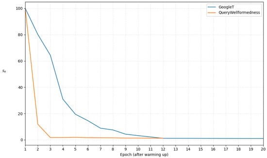
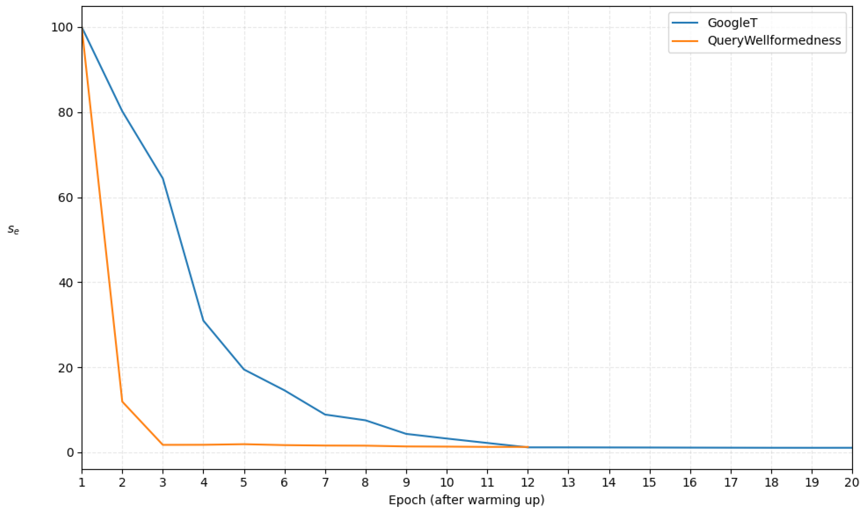
As shown in Figure 2, the selection pressure $s_e$ controls the sharpness of the uncertainty-based sampling distribution. A large selection pressure makes the sampler focus on a smaller set of highly uncertain instances, while a smaller value yields a more spread-out distribution. If this pressure remains too strong, the model may overfit to a narrow subset of difficult or noisy instances.

Figure 2. Change in adaptive selection pressure $s_e$ across epochs. Since $s_e$ is adjusted according to entropy, datasets with faster convergence show a sharper decrease in selection pressure and an earlier expansion of the sampling distribution.

SABI uses the entropy-based selection pressure from SAB:

$$s_e=s_{e_0}{\left(exp\left({\displaystyle \frac{log(1/s_{e_0})}{{entropy}_{e_0}N}}\right)\right)}^{({entropy}_{e_0}-{entropy}_e)N},$$

(15)

where $s_{e_0}$ is the initial selection pressure, ${entropy}_{e_0}$ is the entropy at the beginning of uncertainty-based sampling, and ${entropy}_e$ is the entropy at epoch e.

As entropy decreases during training, the sampling distribution gradually becomes less concentrated. This allows the model to focus on uncertain instances early in training and then progressively include a broader range of training instances. In imbalanced settings, this helps prevent the sampler from over-concentrating on a small set of difficult or noisy examples.

3.7. Computational Complexity

SABI adds three main operations to standard training: maintaining prediction histories, computing uncertainty scores, and constructing the sampling probability. The prediction history requires $O\left(Nq\right)$ memory, where N is the number of training instances and q is the window size. Since q is small in practice, this cost is modest compared with the memory required by the model and mini-batches.

The Gini coefficient is computed once before training, so it does not affect the per-epoch training cost. After the warming-up period, uncertainty scores and sampling probabilities are updated once per epoch. This requires $O\left(N\right)$ operations, or $O(NlogN)$ if sorting is used for ranking or quantization. Compared with the cost of forward and backward propagation, this overhead is relatively small.

Overall, SABI keeps the training procedure close to standard mini-batch optimization while adding a lightweight sampling step that accounts for both uncertainty and class imbalance.

4. Experiment

4.1. Experimental Setup

Performance in classification tasks can vary depending on several factors such as data structure, number of classes, and number of samples. Therefore, to verify the generalizability of SABI, we conduct experiments using 11 different text datasets and 8 image datasets. We perform experiments using text datasets [25,26,27] and image datasets [28] that are commonly used in various studies [29] and benchmarking. As shown in Table 1, the Google datasets [30] exhibit a long-tail distribution among the text datasets. For image data, the CIFAR-10 and CIFAR-100 datasets are modified to have a long-tail distribution according to previous research [31] and then used in the experiments. For datasets that are not pre-divided, about 20% of the data are used for evaluation. The remaining data are then split into 90% for training and 10% for validation.

Table 1. Statistics of the text and image datasets used in the experiments.

Dataset	Train	Valid	Test	Num Class	Gini Coefficient
AG News [32]	108,000	12,000	7600	4	0.0
Biomedical [33]	14,400	1600	4000	20	0.01
Google S [30]	7997	889	2222	152	0.508
Google T [30]	7998	889	2222	152	0.508
Google TS [30]	7997	889	2222	152	0.508
IMDB [25]	20,000	5000	25,000	2	0.0
PAN 19-1, 5 [34]	45	18	468	9	0.0
Query Wellformedness [35]	17,500	3750	3750	2	0.005
SST2 [26]	67,349	872	1821	2	0.05
20News [27]	9051	2263	7532	20	0.04
CIFAR-10 [28]	40,000	10,000	10,000	10	0.0
CIFAR-10 LT 10 [31]	16,344	4087	10,000	10	0.38
CIFAR-10 LT 50 [31]	11,196	2800	10,000	10	0.559
CIFAR-10 LT 100 [31]	9924	2482	10,000	10	0.612
CIFAR-100 [28]	40,000	10,000	10,000	100	0.0
CIFAR-100 LT 10 [31]	15,658	3915	10,000	100	0.35
CIFAR-100 LT 50 [31]	10,086	2522	10,000	100	0.534
CIFAR-100 LT 100 [31]	8677	2170	10,000	100	0.591

The Gini coefficient is computed only once prior to the commencement of training. Therefore, its introduction incurs a negligible one-time computational cost and does not affect the iterative training efficiency of the model, as it is treated as a constant throughout the learning process.

The language model used in our experiments is BERT [36], which was trained for language understanding. We conducted the experiments using the bert-base-uncased model. In addition, for image classification experiments, we use the BEIT model [37,38].

Since we are comparing the recency bias and active bias with SABI, we need to consider several parameters when using recency bias and active bias. Based on previous studies, we conduct experiments with a warming-up period of 10, a sliding window size of 10, and $s_{e_0}$ set to 100.

For the model’s hyperparameters in our experiments, we fix the learning rate at 1 × 10⁻⁵ and use Adam as the optimizer, retaining the default values for the remaining hyperparameters. Since we conduct experiments on various datasets, the maximum batch size was flexibly set according to the characteristics of each dataset, based on the TITAN RTX GPU. For image classification experiments, all input images were resized to 224 × 224 pixels. The batch size is also set to the maximum within the available GPU capacity. Regarding the number of epochs, we apply early stopping, terminating the training if the loss on the validation data does not improve for five consecutive evaluations. We use cross-entropy as the loss function, and the sliding window size is set to a variable size according to the warming-up period.

To assess the performance of the proposed batch sampling method, we conduct a text/image classification task. Since the evaluation is performed on both balanced and imbalanced data, we use the macro F1-score and accuracy as the performance metrics.

To assess the statistical significance of our results, we performed a paired t-test for the means of the performance metrics. For each dataset, we compared SABI against the strongest baselines. A performance improvement was considered statistically significant if the resulting p-value was less than 0.05.

All experiments were conducted with fixed random seeds {40, 41, 42, 43, 44}. The reported results are averaged over repeated runs, with standard deviations reported in Table 2 and Table 3.

Table 2. Performance comparison of different methods across text datasets. The number in parentheses next to each dataset name represents the Gini coefficient. Bold text indicates the highest performance. An asterisk (*) indicates that the improvement of SABI over the second-highest performing method is statistically significant with $p<0.05$.

Method (Gini’s Coef.)	Metrics	Baseline	Active Bias	Recency Bias	Oversample	SAB	SABI
AgNews (0.0)	Acc	93.28 ± 0.07	93.42 ± 0.21	93.65 ± 0.14	93.58 ± 0.09	93.91 ± 0.12	* 93.91 ± 0.12 (+0.26)
	Macro F1	93.31 ± 0.07	93.40 ± 0.20	93.65 ± 0.14	93.59 ± 0.09	93.90 ± 0.12	* 93.90 ± 0.12 (+0.25)
Biomedical (0.01)	Acc	68.32 ± 0.06	70.97 ± 0.15	71.16 ± 0.10	70.64 ± 0.10	71.13 ± 0.09	* 71.31 ± 0.10 (+0.15)
	Macro F1	68.65 ± 0.09	71.12 ± 0.19	71.32 ± 0.15	70.85 ± 0.10	71.34 ± 0.12	* 71.58 ± 0.06 (+0.24)
GoogleS (0.508)	Acc	91.25 ± 0.11	91.44 ± 0.34	92.12 ± 0.20	92.56 ± 0.07	92.40 ± 0.25	92.68 ± 0.15 (+0.12)
	Macro F1	89.22 ± 0.31	89.30 ± 0.42	89.64 ± 0.39	90.44 ± 0.11	89.89 ± 0.23	90.29 ± 0.26 (−0.15)
GoogleT (0.508)	Acc	92.52 ± 0.08	92.64 ± 0.17	92.85 ± 0.03	93.22 ± 0.06	93.16 ± 0.07	* 93.34 ± 0.03 (+0.12)
	Macro F1	88.02 ± 0.14	88.06 ± 0.29	88.35 ± 0.11	89.63 ± 0.20	89.02 ± 0.11	89.51 ± 0.19 (−0.12)
GoogleTS (0.508)	Acc	96.24 ± 0.13	96.18 ± 0.19	95.38 ± 0.11	96.41 ± 0.09	96.12 ± 0.05	* 96.52 ± 0.08 (+0.11)
	Macro F1	93.92 ± 0.25	94.10 ± 0.33	94.17 ± 0.16	94.44 ± 0.10	94.26 ± 0.12	* 94.51 ± 0.14 (+0.07)
IMDB (0.0)	Acc	92.51 ± 0.14	91.63 ± 0.11	92.71 ± 0.06	92.04 ± 0.22	92.82 ± 0.10	* 92.82 ± 0.10 (+0.11)
	Macro F1	92.54 ± 0.14	91.64 ± 0.11	92.72 ± 0.06	92.04 ± 0.22	92.81 ± 0.10	* 92.81 ± 0.10 (+0.09)
PAN19-1 (0.0)	Acc	73.51 ± 0.20	74.24 ± 0.44	75.21 ± 0.25	75.14 ± 0.31	75.77 ± 0.27	* 75.77 ± 0.27 (+0.56)
	Macro F1	59.53 ± 0.32	60.22 ± 0.53	59.37 ± 0.40	58.26 ± 0.49	60.28 ± 0.36	60.28 ± 0.36 (+0.06)
PAN19-5 (0.0)	Acc	53.72 ± 0.21	54.15 ± 0.38	53.54 ± 0.31	54.05 ± 0.38	54.88 ± 0.29	* 54.88 ± 0.29 (+0.73)
	Macro F1	24.06 ± 0.35	28.97 ± 0.51	28.13 ± 0.36	25.01 ± 0.44	29.83 ± 0.36	* 29.83 ± 0.36 (+0.86)
QueryWellformedness (0.005)	Acc	79.82 ± 0.11	81.52 ± 0.13	81.38 ± 0.10	80.89 ± 0.08	81.59 ± 0.07	* 81.73 ± 0.09 (+0.14)
	Macro F1	79.81 ± 0.09	81.44 ± 0.15	81.32 ± 0.10	80.77 ± 0.08	81.49 ± 0.08	* 81.60 ± 0.07 (+0.11)
SST2 (0.05)	Acc	91.12 ± 0.02	91.08 ± 0.08	92.01 ± 0.06	92.04 ± 0.09	92.81 ± 0.02	92.83 ± 0.03 (+0.02)
	Macro F1	91.12 ± 0.04	91.08 ± 0.08	92.01 ± 0.06	92.04 ± 0.08	92.81 ± 0.02	92.83 ± 0.04 (+0.02)
20News (0.04)	Acc	84.48 ± 0.19	84.26 ± 0.23	84.92 ± 0.15	84.40 ± 0.09	85.22 ± 0.18	* 85.88 ± 0.13 (+0.66)
	Macro F1	83.81 ± 0.18	84.35 ± 0.24	83.65 ± 0.21	84.24 ± 0.12	84.53 ± 0.19	* 85.14 ± 0.13 (+0.61)

Table 3. Performance comparison of different methods across image datasets. The number in parentheses next to each dataset name represents the Gini coefficient. Bold text indicates the highest performance. An asterisk (*) indicates that the improvement of SABI over the second-highest performing method is statistically significant with $p<0.05$.

Method (Gini’s Coef.)	Metrics	Baseline	Active Bias	Recency Bias	Oversample	SAB	SABI
CIFAR-10 (0.0)	Acc	95.37$\pm 0.05$	95.78$\pm 0.11$	96.02$\pm 0.06$	95.99$\pm 0.05$	96.43$\pm 0.08$	* 96.43$\pm 0.08$ (+0.41)
	Macro F1	95.36$\pm 0.05$	95.78$\pm 0.10$	96.02$\pm 0.06$	96.00$\pm 0.05$	96.42$\pm 0.08$	* 96.42$\pm 0.08$ (+0.40)
CIFAR-10 LT 10 (0.38)	Acc	93.11$\pm 0.06$	92.80$\pm 0.11$	92.91$\pm 0.07$	92.88$\pm 0.05$	93.31$\pm 0.03$	93.34$\pm 0.04$ (+0.03)
	Macro F1	93.12$\pm 0.06$	92.79$\pm 0.12$	92.91$\pm 0.07$	92.89$\pm 0.05$	93.32$\pm 0.03$	93.36$\pm 0.04$ (+0.04)
CIFAR-10 LT 50 (0.559)	Acc	86.74$\pm 0.10$	84.17$\pm 0.09$	86.25$\pm 0.09$	88.72$\pm 0.03$	88.33$\pm 0.07$	* 88.79$\pm 0.06$ (+0.07)
	Macro F1	86.75$\pm 0.14$	84.18$\pm 0.14$	84.24$\pm 0.10$	88.72$\pm 0.03$	88.33$\pm 0.06$	* 88.79$\pm 0.06$ (+0.07)
CIFAR-10 LT 100 (0.612)	Acc	83.32$\pm 0.12$	79.22$\pm 0.16$	83.76$\pm 0.13$	85.59$\pm 0.08$	84.50$\pm 0.18$	* 85.78$\pm 0.15$ (+0.19)
	Macro F1	83.16$\pm 0.12$	79.03$\pm 0.18$	83.69$\pm 0.15$	85.44$\pm 0.09$	83.34$\pm 0.20$	* 85.61$\pm 0.13$ (+0.17)
CIFAR-100 (0.0)	Acc	78.01$\pm 0.07$	78.46$\pm 0.12$	78.93$\pm 0.10$	78.89$\pm 0.06$	79.28$\pm 0.09$	* 79.28$\pm 0.09$ (+0.35)
	Macro F1	77.97$\pm 0.09$	74.45$\pm 0.12$	78.92$\pm 0.10$	78.89$\pm 0.07$	79.29$\pm 0.09$	* 79.29$\pm 0.09$ (+0.37)
CIFAR-100 LT 10 (0.35)	Acc	63.96$\pm 0.11$	64.52$\pm 0.10$	64.91$\pm 0.17$	67.11$\pm 0.09$	67.32$\pm 0.15$	* 67.49$\pm 0.12$ (+0.17)
	Macro F1	62.68$\pm 0.14$	63.31$\pm 0.13$	63.83$\pm 0.17$	66.71$\pm 0.11$	66.81$\pm 0.16$	* 67.05$\pm 0.13$ (+0.24)
CIFAR-100 LT 50 (0.534)	Acc	48.62$\pm 0.13$	49.13$\pm 0.24$	49.25$\pm 0.23$	52.87$\pm 0.11$	52.47$\pm 0.23$	52.89$\pm 0.19$ (+0.02)
	Macro F1	43.95$\pm 0.16$	44.18$\pm 0.28$	46.31$\pm 0.24$	52.71$\pm 0.10$	47.88$\pm 0.23$	52.54$\pm 0.19$ (−0.17)
CIFAR-100 LT 100 (0.591)	Acc	44.71$\pm 0.08$	45.67$\pm 0.15$	44.52$\pm 0.17$	50.33$\pm 0.06$	49.80$\pm 0.16$	50.09$\pm 0.13$ (−0.24)
	Macro F1	38.23$\pm 0.10$	39.58$\pm 0.22$	39.62$\pm 0.18$	47.10$\pm 0.06$	43.09$\pm 0.19$	46.53$\pm 0.13$ (−0.57)

4.2. Result

To evaluate the proposed method, we conduct experiments under various settings. The baseline for this experiment is the method of training a language model and classifier using the entire training dataset. We conduct experiments using the baseline, Active Bias, Recency Bias, Oversampling, SAB, and SABI.

Table 2 and Table 3 present the overall experimental results for each dataset. It can be seen that SABI, which applies the credal set, achieves higher performance than both SAB and Oversampling in most experiments. In particular, compared to SAB, consistent improvements were observed in both accuracy and macro F1, supporting the effectiveness of the proposed method. While Oversampling achieves high performance on some datasets with a high Gini coefficient, it shows lower performance than SABI on datasets with a low Gini coefficient. This indicates that the Oversampling method is sensitive to the data distribution and is a less robust sampling method. In contrast, SABI achieves competitive average performance across the datasets while maintaining a stable balance between uncertainty-driven sampling and imbalance-aware sampling. Although SABI shows slightly lower performance than Oversampling on a few datasets, these cases indicate that strongly minority-focused sampling can be beneficial in some highly imbalanced settings. Overall, the results suggest that SABI provides a more balanced trade-off across different data distributions rather than uniformly outperforming every baseline in all cases.

From a component-wise perspective, SAB and Oversampling provide useful reference points for analyzing the two main components of SABI. SAB represents the uncertainty-driven component, since it relies on recent prediction instability for sample selection without explicitly incorporating class-frequency information. Oversampling, on the other hand, represents an imbalance-driven strategy that increases the exposure of minority-class instances without considering instance-level uncertainty. The comparison among SAB, Oversampling, and SABI therefore helps show that SABI benefits from combining uncertainty-driven sampling with imbalance-aware sampling, rather than relying on either signal alone.

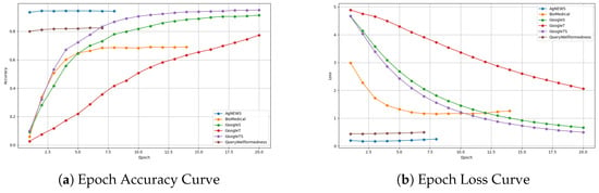
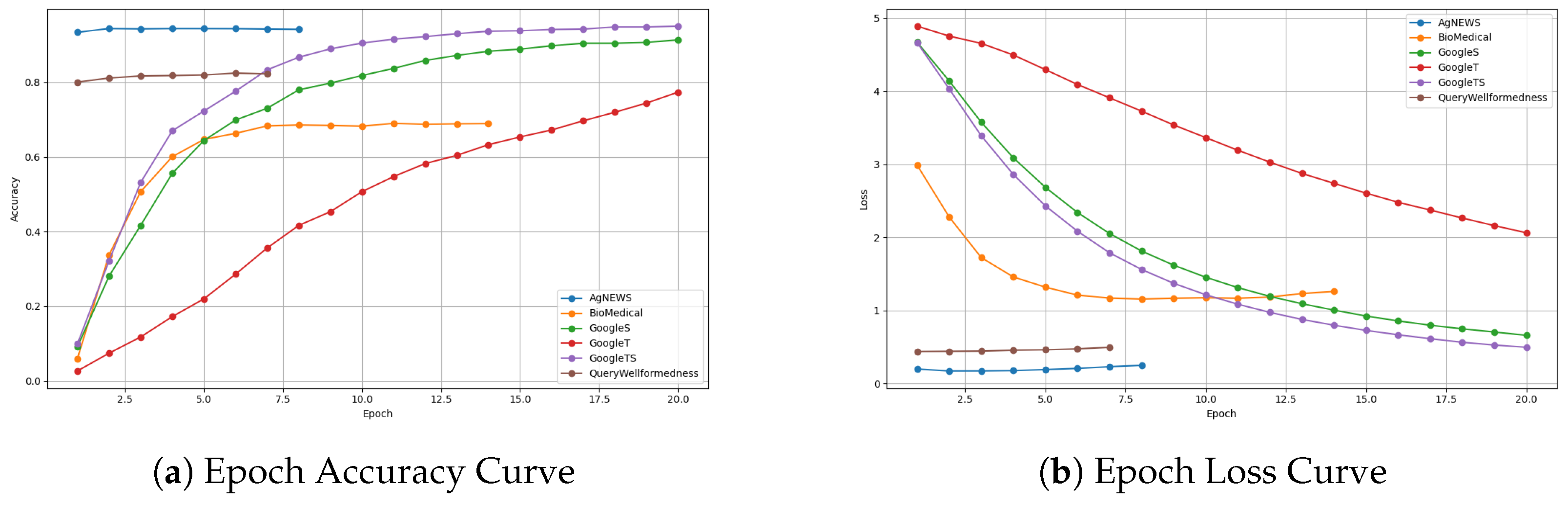
In the case of active bias [19] and recency bias [7], the warming-up period was set to 10 iterations for all data according to previous studies. However, since these methods apply the same warming-up period even when the process could end in fewer than 10 iterations, the sample selection time may be delayed and overfitting may occur. In contrast, SAB and SABI determine the warming-up period adaptively based on changes in loss. As shown in Figure 3, this approach allows for flexible adaptation to data that converges in fewer epochs or requires a longer warming-up period due to its characteristics. As observed for AgNews and QueryWellformedness, SAB and SABI achieve improved performance under this adaptive warming-up strategy.

Figure 3. Accuracy and loss curves across epochs. Different datasets exhibit different learning dynamics, which motivates the use of an adaptive warming-up period.

For long-tail data with a Gini coefficient higher than 0.5, SAB shows better performance than active and recency bias, but lower performance compared to methods such as Oversampling that place greater sampling emphasis on minority classes. However, SABI uses a sampling method that considers the probabilities from both SAB and Oversampling. As a result, this sampling method is able to effectively distinguish between cases where errors occur simply due to small data size and cases where errors occur due to the inherent difficulty of the data. Experimental results show that, on average, SABI improves accuracy and macro F1 by 0.22% and 0.75%, respectively, compared to SAB. Compared to Oversampling, improvements of 0.98% and 0.17% were observed, respectively. These results indicate that SABI remains competitive across both nearly balanced and long-tailed settings. In highly imbalanced datasets, Oversampling can sometimes achieve stronger performance by aggressively emphasizing minority classes. However, SABI provides a complementary advantage by combining minority-aware sampling with instance-level uncertainty, which helps maintain a balanced performance profile across different class-frequency regions.

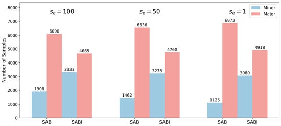
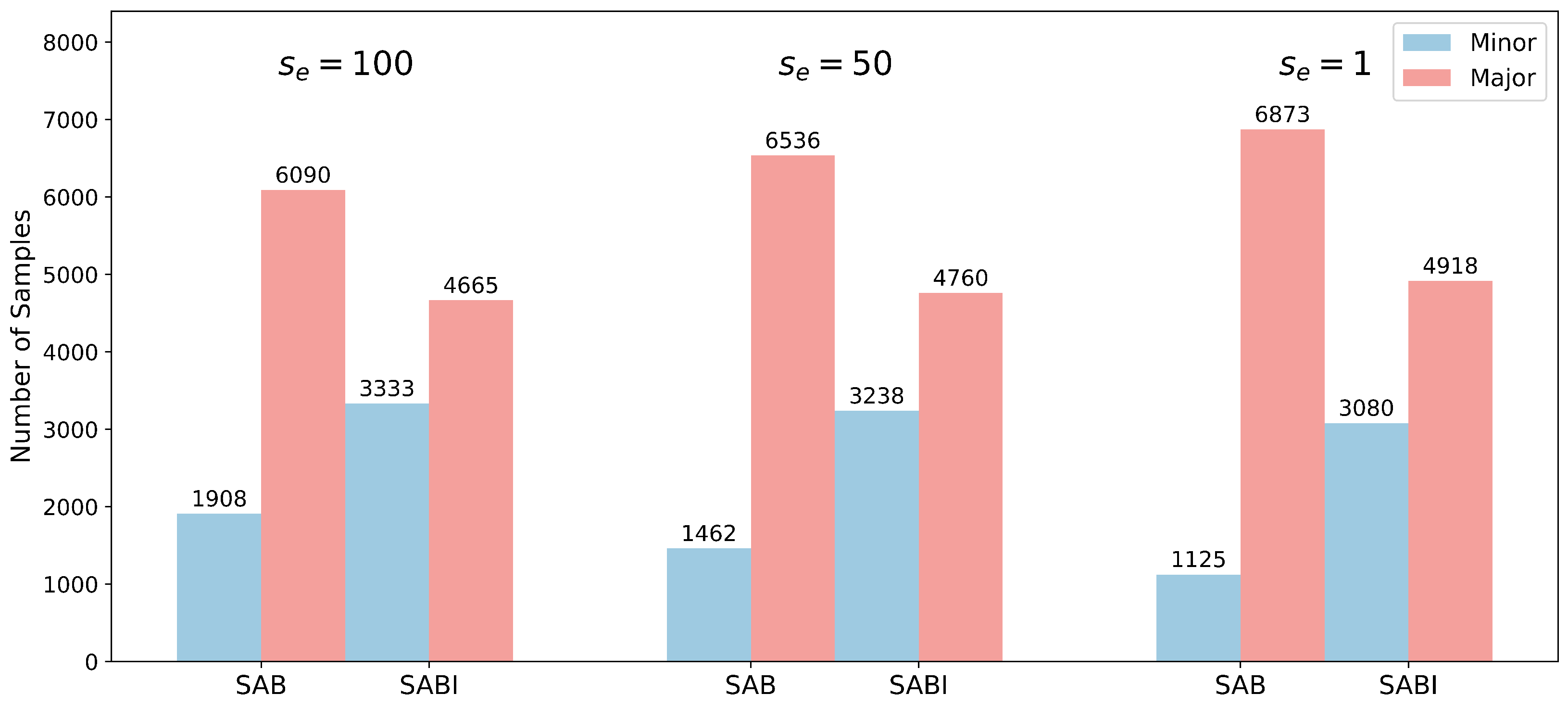
Figure 4 shows the sampling differences between SAB and SABI. We were curious about what causes the performance gap between SAB and SABI in class-imbalanced data. The figure compares the number of samples drawn from major and minor classes at the beginning of training ($s_e=100$), in the middle, and at the end. We can see that SABI maintains a smaller gap between major and minor classes compared to SAB. Therefore, maintaining a certain ratio between the two appears to help improve performance.

Figure 4. Sampling differences between SAB and SABI. The number of samples drawn from major and minor classes at the beginning, middle, and end of training is compared.

Table 4 summarizes macro F1 on GoogleTS under a head/body/tail label split (30/92/30 labels). Oversampling achieves the highest Tail score, while SAB and SABI are stronger on Head and Body, where most labels are. Importantly, SABI closes much of SAB’s gap on Tail—reaching a level close to Oversampling without giving up its gains on Head/Body. SABI offers the most even trade-off across groups rather than optimizing a single region.

Table 4. Macro F1 on GoogleTS by label group. SABI leads on Head/Body and remains competitive on Tail.

Method	Head	Body	Tail
SABI	0.9959	0.9402	0.7516
Over	0.9810	0.9334	0.7563
SAB	0.9956	0.9352	0.7200
Default	0.9813	0.9328	0.7182

This group-wise analysis provides a more detailed view of minority-class behavior than aggregate accuracy and macro F1 alone. Although Oversampling obtains the highest Tail score, SABI substantially improves the Tail score over SAB while maintaining stronger Head and Body performance. This suggests that SABI improves minority-class exposure without excessively sacrificing performance on frequent classes.

The primary memory overhead of Ours comes from storing the “label history” for each of the N samples over a sliding window of size q. This results in an additional memory requirement of $O(N·q)$, which scales linearly with the dataset size. Given that the model parameters and data batches occupy the vast majority of GPU memory, this overhead is practically negligible. As shown in Table 5, the memory consumption of Ours (4165.77 MB) represents a mere 0.19% increase compared to the baseline (4157.88 MB). This empirically confirms that the memory overhead required for storing the label history is negligible and does not pose a practical limitation for deploying our method on standard hardware.

Table 5. Average memory used. All units are in MB.

Methods	Baseline	Active	Recency	Oversample	SAB	SABI
Total Memory used (MB)	4157.88	4169.41	4165.26	4160.89	4162.71	4165.77

SABI introduces an additional computational step at the beginning of each epoch. This step involves calculating uncertainty for all N training samples, which has a complexity of $O\left(N\right)$, and then sorting or quantizing these uncertainties, which takes $O(NlogN)$. Since this calculation is performed once per epoch, the total overhead is marginal compared to the cost of the training iterations themselves. The Gini coefficient calculation is a one-time $O\left(N\right)$ operation performed before training begins and thus adds no iterative overhead.As shown in Table 6, SABI introduces a ‘Sampling Time’ overhead of 78.5 s for data selection, this strategic selection leads to faster model convergence. This increased efficiency is evident as the core ‘Training Time’ (233.4 s) is actually 3.6% shorter than the standard baseline training (242.2 s). Therefore, while the total wall-clock time is slightly longer, the model reaches its optimal performance in fewer training updates, demonstrating a more efficient learning process.

Table 6. Sampling time, training time, and total time for each algorithm. All units are in seconds.

Methods	Baseline	Active	Recency	Oversample	SAB	SABI
Sampling Time (s)	-	78.3	78.6	-	78.5	78.5
Training Time (s)	242.2	243.3	233.5	233.6	233.2	233.4
Total Time (s)	242.2	321.6	312.1	233.6	311.7	311.9

5. Conclusions

In this paper, we proposed SABI, a data sampling strategy designed to effectively handle datasets with long-tail distributions characterized by high Gini coefficients. SABI is inspired by credal set reasoning, but is designed as a practical sampling strategy rather than a full credal classification framework. It jointly considers data uncertainty and the overall class distribution to better reflect each sample’s contribution to learning. This design enables more effective mini-batch construction. As shown in Table 2, SABI consistently outperforms the baseline methods on most datasets. For example, on the 20News dataset, SABI achieved a Macro F1 score of 85.14, and the improvement over the next best method, SAB, was statistically significant ($p<0.05$). These results indicate that the performance gains are attributable to the proposed sampling strategy.

In future work, we plan to extend this method to more complex settings, such as multi-label classification, where inter-label dependencies exist and class imbalance is often more severe.

References

- Krawczyk, B. Learning from imbalanced data: Open challenges and future directions. Prog. Artif. Intell. 2016, 5, 221–232. [Google Scholar] [CrossRef] [Scilit]
- Chawla, N.V.; Bowyer, K.W.; Hall, L.O.; Kegelmeyer, W.P. SMOTE: Synthetic minority over-sampling technique. J. Artif. Intell. Res. 2002, 16, 321–357. [Google Scholar] [CrossRef] [Scilit]
- Settles, B. Active Learning Literature Survey. 2009. Available online: http://digital.library.wisc.edu/1793/60660 (accessed on 3 May 2026).
- Yang, L.; Jiang, H.; Song, Q.; Guo, J. A Survey on Long-Tailed Visual Recognition. Int. J. Comput. Vis. 2022, 130, 1837–1872. [Google Scholar] [CrossRef] [Scilit]
- Walley, P. Statistical Reasoning with Imprecise Probabilities. 1990. Available online: https://philpapers.org/rec/WALSRW (accessed on 3 May 2026).
- Benavoli, A.; Azzimonti, D.; Piga, D. Skew Gaussian processes for classification. Mach. Learn. 2020, 109, 1877–1902. [Google Scholar] [CrossRef] [Scilit]
- Song, H.; Kim, M.; Kim, S.; Lee, J.G. Carpe Diem, Seize the Samples Uncertain “at the Moment” for Adaptive Batch Selection. In Proceedings of the 29th ACM International Conference on Information & Knowledge Management, Virtual, 19–23 October 2020. [Google Scholar]
- Katharopoulos, A.; Fleuret, F. Not All Samples Are Created Equal: Deep Learning with Importance Sampling. In Proceedings of the International Conference on Machine Learning, Stockholm, Sweden, 10–15 July 2018. [Google Scholar]
- Wallace, B.C.; Small, K.; Brodley, C.E.; Trikalinos, T.A. Class Imbalance, Redux. In Proceedings of the 2011 IEEE 11th International Conference on Data Mining; IEEE: New York, NY, USA, 2011; pp. 754–763. [Google Scholar]
- Kubát, M.; Matwin, S. Addressing the Curse of Imbalanced Training Sets: One-Sided Selection. In Proceedings of the International Conference on Machine Learning, Nashville, TN, USA, 8–12 July 1997. [Google Scholar]
- Mohammed, R.; Rawashdeh, J.; Abdullah, M. Machine Learning with Oversampling and Undersampling Techniques: Overview Study and Experimental Results. In Proceedings of the 2020 11th International Conference on Information and Communication Systems (ICICS); IEEE: New York, NY, USA, 2020; pp. 243–248. [Google Scholar]
- Qiao, X.; Liu, Y. Adaptive Weighted Learning for Unbalanced Multicategory Classification. Biometrics 2009, 65, 159–168. [Google Scholar] [CrossRef] [Scilit] [PubMed]
- Gawlikowski, J.; Tassi, C.R.N.; Ali, M.; Lee, J.; Humt, M.; Feng, J.; Kruspe, A.M.; Triebel, R.; Jung, P.; Roscher, R.; et al. A survey of uncertainty in deep neural networks. Artif. Intell. Rev. 2021, 56, 1513–1589. [Google Scholar] [CrossRef] [Scilit]
- Li, C.; Li, K.; Ou, Y.; Kaplan, L.M.; Jøsang, A.; Cho, J.H.; Jeong, D.H.; Chen, F. Hyper Evidential Deep Learning to Quantify Composite Classification Uncertainty. arXiv 2024, arXiv:2404.10980. [Google Scholar] [CrossRef] [Scilit]
- Loshchilov, I.; Hutter, F. Online batch selection for faster training of neural networks. In Proceedings of the the 4th International Conference on Learning Representation, San Juan, Puerto Rico, 2–4 May 2016. [Google Scholar]
- Kumar, M.P.; Packer, B.; Koller, D. Self-Paced Learning for Latent Variable Models. In Proceedings of the Neural Information Processing Systems, Vancouver, BC, Canada, 6–9 December 2010. [Google Scholar]
- Zhou, T.; Bilmes, J.A. Minimax Curriculum Learning: Machine Teaching with Desirable Difficulties and Scheduled Diversity. In Proceedings of the International Conference on Learning Representations, Vancouver, BC, Canada, 30 April–3 May 2018. [Google Scholar]
- Song, H.; Kim, S.; Kim, M.; Lee, J.G. Ada-Boundary: Accelerating DNN Training via Adaptive Boundary Batch Selection. Mach. Learn. 2020, 109, 1837–1853. [Google Scholar] [CrossRef] [Scilit]
- Chang, H.S.; Learned-Miller, E.G.; McCallum, A. Active Bias: Training More Accurate Neural Networks by Emphasizing High Variance Samples. In Proceedings of the Neural Information Processing Systems, Long Beach, CA, USA, 4–9 December 2017. [Google Scholar]
- Choi, S.; Oh, J.; Cha, J.W. SAB: Self-Adaptive Bias. AI 2024, 5, 2761–2772. [Google Scholar] [CrossRef] [Scilit]
- Shi, X.; Chen, Z.; Wang, H.; Yeung, D.Y.; Wong, W.K.; Chun Woo, W. Convolutional LSTM Network: A Machine Learning Approach for Precipitation Nowcasting. In Proceedings of the Neural Information Processing Systems, Montreal, QC, Canada, 7–12 December 2015. [Google Scholar]
- Vaswani, A.; Shazeer, N.M.; Parmar, N.; Uszkoreit, J.; Jones, L.; Gomez, A.N.; Kaiser, L.; Polosukhin, I. Attention is All you Need. In Proceedings of the Neural Information Processing Systems, Long Beach, CA, USA, 4–9 December 2017. [Google Scholar]
- Chae, Y.; Davidson, T.R. Large Language Models for Text Classification: From Zero-Shot Learning to Instruction-Tuning. Sociol. Methods Res. 2025, 55, 501–567. [Google Scholar] [CrossRef] [Scilit]
- Sun, X.; Li, X.; Li, J.; Wu, F.; Guo, S.; Zhang, T.; Wang, G. Text Classification via Large Language Models. In Proceedings of the Conference on Empirical Methods in Natural Language Processing, Singapore, 6–10 December 2023. [Google Scholar]
- Maas, A.L.; Daly, R.E.; Pham, P.T.; Huang, D.; Ng, A.Y.; Potts, C. Learning Word Vectors for Sentiment Analysis. In Proceedings of the 49th Annual Meeting of the Association for Computational Linguistics: Human Language Technologies, Portland, OR, USA, 19–24 June 2011; Association for Computational Linguistics: Stroudsburg, PA, USA, 2011; pp. 142–150. [Google Scholar]
- Socher, R.; Perelygin, A.; Wu, J.; Chuang, J.; Manning, C.D.; Ng, A.; Potts, C. Recursive Deep Models for Semantic Compositionality Over a Sentiment Treebank. In Proceedings of the Conference on Empirical Methods in Natural Language Processing, Grand Hyatt, WA, USA, 18–21 October 2013. [Google Scholar]
- Lang, K. NewsWeeder: Learning to Filter Netnews. In Proceedings of the International Conference on Machine Learning, Tahoe, CA, USA, 9–12 July 1995. [Google Scholar]
- Krizhevsky, A. Learning Multiple Layers of Features from Tiny Images. 2009. Available online: https://www.cs.utoronto.ca/~kriz/learning-features-2009-TR.pdf (accessed on 3 May 2026).
- Zhang, D.; Nan, F.; Wei, X.; Li, S.W.; Zhu, H.; McKeown, K.; Nallapati, R.; Arnold, A.O.; Xiang, B. Supporting Clustering with Contrastive Learning. In Proceedings of the North American Chapter of the Association for Computational Linguistics, Online, 6–11 June 2021. [Google Scholar]
- Yin, J.; Wang, J. A model-based approach for text clustering with outlier detection. In Proceedings of the 2016 IEEE 32nd International Conference on Data Engineering (ICDE); IEEE: New York, NY, USA, 2016; pp. 625–636. [Google Scholar]
- Cui, Y.; Jia, M.; Lin, T.Y.; Song, Y.; Belongie, S.J. Class-Balanced Loss Based on Effective Number of Samples. In Proceedings of the 2019 IEEE/CVF Conference on Computer Vision and Pattern Recognition (CVPR); IEEE: New York, NY, USA, 2019; pp. 9260–9269. [Google Scholar]
- Zhang, X.; LeCun, Y. Text Understanding from Scratch. arXiv 2015, arXiv:1502.01710. [Google Scholar]
- Xu, J.; Xu, B.; Wang, P.; Zheng, S.; Tian, G.; Zhao, J. Self-Taught Convolutional Neural Networks for Short Text Clustering. Neural Netw. Off. J. Int. Neural Netw. Soc. 2017, 88, 22–31. [Google Scholar] [CrossRef] [Scilit] [PubMed]
- Kestemont, M.; Stamatatos, E.; Manjavacas, E.; Daelemans, W.; Potthast, M.; Stein, B. Overview of the Cross-domain Authorship Attribution Task at PAN 2019. In Proceedings of the Conference and Labs of the Evaluation Forum, Lugano, Switzerland, 9–12 September 2019. [Google Scholar]
- Faruqui, M.; Das, D. Identifying Well-formed Natural Language Questions. In Proceedings of the EMNLP, Brussels, Belgium, 31 October–1 November 2018. [Google Scholar]
- Devlin, J.; Chang, M.W.; Lee, K.; Toutanova, K. BERT: Pre-training of Deep Bidirectional Transformers for Language Understanding. In Proceedings of the North American Chapter of the Association for Computational Linguistics, Minneapolis, MN, USA, 2–7 June 2019. [Google Scholar]
- Bao, H.; Dong, L.; Wei, F. BEiT: BERT Pre-Training of Image Transformers. arXiv 2021, arXiv:2106.08254. [Google Scholar]
- Deng, J.; Dong, W.; Socher, R.; Li, L.J.; Li, K.; Fei-Fei, L. Imagenet: A large-scale hierarchical image database. In Proceedings of the 2009 IEEE Conference on Computer Vision and Pattern Recognition; IEEE: New York, NY, USA, 2009; pp. 248–255. [Google Scholar]
Disclaimer/Publisher’s Note: The statements, opinions and data contained in all publications are solely those of the individual author(s) and contributor(s) and not of MDPI and/or the editor(s). MDPI and/or the editor(s) disclaim responsibility for any injury to people or property resulting from any ideas, methods, instructions or products referred to in the content. |
© 2026 by the authors. Licensee MDPI, Basel, Switzerland. This article is an open access article distributed under the terms and conditions of the Creative Commons Attribution (CC BY) license.