


Abstract
Rotor systems are basic in power generation, mechanical, and many other energy equipment and industrial fields. The smooth operation of equipment is linked to the successful operation of technological processes and the safe operation of working equipment. Working conditions nowadays are characterized by intensive rotation speeds, complex structures, and dynamic loads, contributing to different mechanical faults. Detecting such defects in the preliminary stages is inadequate, which could lead to emergencies, high economic loss, and reduced equipment life. Several modern diagnosis methods are widely utilized to monitor the condition in real-time mode, such as vibration parameter analysis, temperature deviation analysis, acoustic emission analysis, and other operational parameter analyses, to avoid the possibility of rotor failure. Some techniques like the vibration signal analysis method, spectral analysis, thermography, ultrasound diagnosis, and machine learning algorithms for predicting failure are of particular interest among them. These techniques allow the defects to be identified immediately and constitute effective preventive maintenance plans, thus significantly enhancing the reliability and economic efficiency of the rotor system operations. This current work is devoted to studying modern diagnostic methods of rotor systems, considering the areas of their realization that are used. This review discusses the theory of the applied methods, advantages, limitations, and the perspective of their further development in innovation integration. It aims to critically analyze and comprehensively systematize methods for energy-consuming rotor equipment condition monitoring that will enhance the efficiency of managing technical conditions for the main components of modern energy systems.
1. Introduction
Rotary machines (pumps, compressors, turbines, turbopump units, etc.) ensure power equipment’s performance, reliability, and energy efficiency, especially in power generation, the oil and gas industry, and renewable energy.
This article uses the terms “classical methods” and “modern methods” to distinguish between fundamentally different approaches to fault diagnosis. The distinction between classical and modern methods in fault diagnosis essentially relies on the computational approach taken and the level of automation involved. Classical methods primarily employ analytical modeling and numerical calculations, often requiring complex physical models and substantial computational power to solve complex mathematical equations. Modern approaches either extend classical methods with artificial intelligence (AI) and machine learning (ML) techniques or are mainly based on them. Thus, contemporary methods are used not just for fault prediction and classification but also to cut down on the computational complexity of analytical techniques.
Certainly, classical methods are still an essential and powerful tool for solving diagnostics problems, but they have a number of limitations, such as high sensitivity to input parameters, scatter or noise, modeling errors, and initial settings. Other limitations are rapid computational cost growth, vulnerability to variations in initial conditions, and difficulty scaling. Moreover, because of these limitations, the mathematical models that describe the system are often simplified, which inevitably diminishes the accuracy of the predictions and the range of conditions under which the approach can be reliably applied.
The study by [1] proposes a new index for detecting blade-to-case contact (rub-impact), demonstrating effectiveness in numerical experiments. However, the model on which it is tested is oversimplified: the rotor stiffness is constant, the bearings are perfectly symmetrical, and temperature- or friction-induced nonlinearities are not considered. As a result, the method is limited to a narrow set of cases and is unlikely to be scalable to complex multi-defect scenarios.
The research work by [2] is also a prime example of the successful use of finite element modeling but with similar limitations. The algorithms process “pure” signals without considering noise, temperature effects, or the gradual deterioration of structural elements.
The work by [3] presents techniques for damage detection in rotary systems. The methods rely on a simple beam model that, while useful for the initial detection of defects, does not account for nonlinearities, asymmetric mass distributions, or variations of elastic moduli characteristic of wear that exist in real machines.
The research by [4] presents a detailed model of a local defect in the inter-rotor bearing. The model considers nonlinear dynamic effects, but symmetrical rotor structures with constant rotation speed are used. All boundary conditions are fixed and do not consider the actual mechanical wear or thermal expansion of the shaft—that is, the model is isolated from variables typical of industrial systems.
The work by [5] assesses the capability of the fast Fourier transform (FFT) for simple fault detection scenarios, demonstrating fast spectral evaluation and easy implementation. However, FFT exhibits low sensitivity to complex, nonstationary signals. The authors do not address multi-fault discrimination.
The paper by [6] deals with linear and nonlinear performance analyses of hydrodynamic bearings. The authors use models based on the Reynolds equation but do not consider the effects of variable lubricant viscosity, thermal effects, or load asymmetry. Moreover, all material properties (stiffness, damping) are assumed to be constant. Thus, although the modeling is detailed from a geometrical point of view, it is limited in physical accuracy.
The work by [7] presents a complex nonlinear model of a rotor–disk system that considers large deflections and even chaotic regimes. However, the authors do not model physically realistic boundary conditions. In particular, the supports’ stiffness and the rotor’s thermal expansion are not considered.
Another work that considers the investigation of nonlinear processes [8] develops a hybrid finite element modeling (FEM) analytical cluster model that accurately captures nonlinear field distributions in induction motors. However, it demands detailed geometric and material data, making it challenging to apply in cases where such information is unavailable. The high computational complexity also limits its use in real-time diagnostics.
The work by [9] introduces topological fractal multi-resolution analysis (TFMRA) for smart machinery fault diagnosis, which uses a combination of optimization and classification methods under wavelet structures and shows high robustness to signal nonlinearities. However, TFMRA is computationally intensive, making real-time deployment challenging. The study also omits a sensitivity analysis of parameter selection.
In the last decade, many novel analytical methods have been developed that could be applied to machine diagnostics. The work by [10] proposes filtered and extended Park’s vector approaches that detect broken rotor bars independently of slot count. However, these methods only target bar faults and fail to detect other defect categories. Their performance under load transients has also not been investigated.
The work by [11] combines Hilbert, Gabor, and Fourier transforms for rotor health monitoring, offering intuitive phase/amplitude insights. However, it is sensitive to high-frequency noise and requires preprocessing. The effect of sensor bandwidth limitations is not discussed.
The main research gaps in these studies include the lack of comprehensive physical modeling, inadequate consideration of real-world boundary conditions, oversimplified AI diagnostics, and insufficient scalability for industrial applications in the power industry and related enterprises, such as incomplete consideration of actual boundary conditions, such as support stiffness and thermal expansion [4,7]; ignoring anisotropy of bearing stiffness, friction-induced nonlinearity, and temperature effects [1]; lack of comprehensive physical modeling, e.g., variable lubricant viscosity, thermal effects, and asymmetric loads [6]; assuming perfectly elastic contact and neglecting micro-roughness, wear, lubrication effects, and potential plastic deformations [12]; oversimplification of machine learning models [13,14] and ignoring signal noise [15]; using simplified beam models that neglect nonlinearities, asymmetric mass distributions, and variations in material properties [2,3].
Modern methods, such as methods based on artificial intelligence (AI) or machine learning (ML), are free of most limitations of classical techniques. They do not need a strict analytical process description to model it. Nevertheless, AI/ML-based methods typically require large, well-labeled datasets, are prone to overfitting and domain-shift errors, and often behave as “black boxes”, which complicates certification or root cause analysis.
Such a critical problem as the contact of the rotor with the bearing in the presence of gaps is considered in his work by [12]. The author proposes a new FEM model that includes geometric aspects of the contact. However, the contact is modeled as perfectly elastic without considering the micro-roughness of the surfaces or wear. Lubricating properties and possible plastic deformations of the contact zones are also not included. Accordingly, the simulation results will differ significantly from the real environment. AI and ML methods are increasingly used in today’s technological trends. However, despite their impressive computational efficiency, they are often disconnected from physical reality, as the models are trained on artificial data created in a controlled environment.
A review article by [13] provides a detailed analysis of the current AI methods used for rotor diagnostics. The authors note that most of these models are built on synthetic or small laboratory datasets. In particular, the algorithms do not consider variable loads, material degradation, or long-term operational effects and are usually not validated on actual production equipment.
The study by [15] presents an approach to state diagnosis using convolutional neural networks. The model achieves high accuracy in detecting defects but is trained on data with a fixed configuration and does not consider multi-physical interactions (e.g., thermal fluctuations and mechanical loading). Similar to many others, this approach assumes that the system’s state is static and invalid in a real machine.
The work by [16] presents a multi-input convolutional neural network (CNN) framework that fuses multiple image-based transforms for mechanical fault classification with high accuracy. However, training requires large labeled datasets and significant hardware resources. The authors also do not discuss the interpretability of the learned features.
Machine learning is becoming widely adopted in diagnostics. For instance, the study by [17] introduces an advanced large-language-model (LLM)-optimized wavelet packet transformation (WPT) framework for early fault prediction in synchronous condensers, integrating intelligent parameter optimization with multi-head attention (MHA) gated recurrent unit (GRU) for temporal pattern recognition (TPR). This approach achieved a diagnostic accuracy of 98.7% and demonstrated significant reductions in false alarm rates and processing time. However, the reliance on high-quality, labeled data and substantial computational resources presents challenges for real-time industrial deployment. The method does not directly address residual life prediction or uncertainty quantification.
Another work that conducted machine learning [18] applies Bayesian hyperparameter optimization (BHO) to a multilayer perceptron (MLP) model for broken-bar fault diagnosis, resulting in improved classification accuracy. However, the optimization process is computationally expensive in large parameter spaces. In addition, the method’s robustness under noisy measurement conditions remains untested.
Finally, an in-depth review of rotor diagnostics from an AI methods standpoint was provided by [14]. Although the paper exhibits a multitude of algorithms, the authors highlight that most studies were conducted using vibration data obtained under simple and idealized conditions. AI models do not accommodate boundary effects, nonlinearities, adaptive time-varying characteristics, or other essential aspects, severely restricting their validity in any real engineering system.
Another class of modern techniques is formed by uncertainty quantification (UQ) methods. They purposely propagate parameter scatter—probabilistic (Monte Carlo, polynomial chaos) or non-probabilistic (interval, fuzzy, evidence)—through the dynamic model and deliver confidence bands or guaranteed envelopes for health metrics like critical speeds and vibration amplitudes. This capability benefits applications such as setting adequate alarm limits, prioritizing leading parameters, optimizing sensor placement, and supporting risk-informed maintenance or design optimization. Yet, UQ techniques have inherent limitations: probabilistic formulations may suffer from the curse of dimensionality and need trustworthy probability distributions, whereas interval or fuzzy counterparts are generally conservative and may cause overly large safety margins; in addition, most approaches depend on surrogate models, whose quality significantly affects accuracy.
In the study by [19], the authors present a state-of-the-art review of uncertainty analysis of rotating machinery, classifying probabilistic, interval, and hybrid approaches and relate them to crack, rub-impact, and misalignment issues. The paper summarizes 150+ references in a decision tree, linking data availability, model intrusiveness, and computational costs, and cites case studies where surrogate-based polynomial chaos expansion (PCE) cuts the runtime by 10–100× without a loss of accuracy. It also draws attention to new demands, such as firm control of active magnetic bearings and Bayesian model updates with sparse measurements. However, the study is descriptive only; no novel standards, standard measures, or test validations are presented. Thus, numerical comparisons between competing approaches and their viability for real applications are still open problems.
In another paper [20], the authors compare the efficiency of the stochastic polynomial chaos surrogate method and the interval optimization method for predicting sheet metal springback. With a third-order polynomial on a sparse Gauss–Legendre grid, they show that Monte Carlo statistics are approximated using only 625 complete FEM runs, while the interval branch offers worst-case bounds more than twice as wide. The study underscores that tooling clearance dominates output variability (about 99%), which confirms the value of UQ in process calibration. However, the approach is demonstrated only with four uncertain parameters and one forming process, and thus, extends to highly nonlinear, multi-process workflows that are untested. Experimental evidence is not presented, and the method does not address defect-driven uncertainties such as die wear or material thinning.
An interval modal superposition method (IMSM) that propagates bounded uncertainties in disk unbalance and bearing stiffness through a two-disk aero-engine rotor model was examined in the work [21]. IMSM reduces the central processing unit (CPU) time from 2 · 105 s to 50 s while enclosing Monte Carlo envelopes within 1%. Its companion, the interval perturbation module (IPM), produces closed-form critical-speed bands. The method is appealing for setting conservative alarm thresholds and quick, data-poor design audits. The sensitivity to the number of retained modes, the conservative widening of response intervals, and the exclusion of parameter correlations and physical defects are among the disadvantages. Therefore, more research is required to extend to high-dimensional uncertainty spaces or nonlinear fault features (such as breathing cracks).
The literature shows that classical and modern techniques each address different parts of the diagnostic challenge, yet neither alone delivers a complete, universally applicable solution for high-power rotor equipment operating under real-world uncertainties. Therefore, this review aims to critically analyze and comprehensively systematize methods for energy-consuming rotor equipment condition monitoring that will enhance the efficiency of the management of the technical conditions’ management of the main components of modern energy systems.
2. Research Methodology
2.1. Analysis of the Most Common Problems in the Diagnostics of the Rotor System
This section offers an analysis of the most common problems in the diagnostics of rotor systems and possible ways to solve these problems, including experiences from the papers that have been observed. The information is summarized in tables for convenient usage purposes. This information can help researchers define the required methodological background for further research.
The most common issues in rotor systems and methods to solve them are summarized in Table 1.
Table 1.
Summary of the most common issues in rotor systems and methods to solve them.
The following subsections offer a comprehensive overview of some of the existing research that addresses the problem provided. The section is divided into subsections for specific issues to make it more convenient. For each paper that has been reviewed, the general concept of the research, the method used by the authors to investigate the problems provided, and the limitations of their solutions are provided.
2.2. Unbalance
Unbalance [65] is among the most common issues in rotating equipment due to irregular mass distribution around the rotation axis. The primary causes are errors during manufacturing, component wear, non-homogeneous material buildup, and mechanical damage [66]. The consequences of unbalance include increased vibrations, bearing wear, support structure loads, and potential failure hazards. Timely detection and balance correction are essential for maintaining rotating equipment’s stable and secure operation.
The study by [14] presents three varying methods of obtaining imbalance. The methods apply to fine-tuning the model parameters so that unbalanced computed values agree with the measured values under equivalent conditions in the physical model. Equivalent loads were adjusted until the eccentricity of the individual unbalance matched the measured value in the first method. The minimization of the difference between the actual and approximate eccentricity values was achieved using the least squares method:
where and are the theoretical and experimental values of the equivalent loads, respectively.
Since there were substantial errors in the determined parameters, the method was refined by reducing the effect of modal expansion, thereby reducing the error due to this effect. The refined method showed a considerable reduction in error compared to the original process. The third approach, however, seeks to minimize the amplitudes of vibration rather than the loads [14]:
where j is the location of measured vibrations; is the vibrations calculated at location j with the fault at location i; is the vibrations measured at location j.
In this case, the varied parameters are the values of equivalent loads applied in the model at damage locations. This method yielded the best outcomes; nevertheless, error levels were intolerably high for some cases. The inherent linearity of the equivalent loads in the model can explain the significant errors obtained. One improvement to this approach can be the application of nonlinear laws in modeling the equivalent loads. Further, the application of nonlinear relationships between the equivalent loads and damping, as well as stiffness, can also lead to producing improved results by taking into consideration the inherent effects due to imbalance.
Figure 1 presents the equivalent vertical loads estimated in the system and the FFT of the vertical forces at a specific node.
Figure 1.
Amplitude–frequency response of the system. Adopted from [14].
Diagnostic models of unbalance tend to place it as a point defect, whereas in nature, depending on the underlying cause, the unbalance can be distributed. The study by [22] examines a diagnostic and balancing method for distributing unbalance under the influence of rotor shaft bending. The authors believe that discrete value modeling of rotor bending-induced imbalance is not precise enough and cannot adequately characterize the phenomenon’s nature. To counter this issue, a model is proposed in which unbalance is treated as a continuously distributed value along the rotor shaft:
where X(z) is the projection of the global eccentricity curve on the x–z plane; Y(z) is the projection of the global eccentricity curve on the y–z plane; , are the polynomial coefficients.
The magnitude of the unbalance depends on the value of the local deflection; therefore, cubic interpolation of rotor deflection was used to calculate the distribution function of unbalance. Sensor measurement data and a finite element model (FEM) of the rotor were used in computing the values of deflections. Forces caused by unbalance were calculated via so-called eccentricity coefficients, which are dependent on the deflection function. Following the distributed unbalanced force function, compensation point masses were calculated. An unbalanced assessing criterion was gained, i.e., the sum of the two Euclidean norms of these functions in planes [22]:
The proposed technique was verified experimentally. The results were consistent with those of the simulations. Moreover, balancing masses derived from the proposed technique decreased the system’s response to figures near the values calculated. Among the research, the outcomes increased modeling accuracy over discrete unbalanced models and offered a criterion-based method for rotor suitability assessment. However, for the approach to be applied, some conditions in measurement need to be met: sensors are at equal intervals, which is not invariably possible in actual rotors. Also, the model does not account for the masses and corresponding unbalances of the disks.
Figure 2 presents the estimated distributed unbalanced eccentricity values for both the X and Y axes.
Figure 2.
Estimated unbalance eccentricity amplitudes in different planes. Adopted from [22].
Mechanical damage to rotor sections can lead to material chipping and imbalance. Therefore, it can be assumed that localizing such damage determines the position of the imbalance. The study by [23] does not connect directly to rotor dynamics but considers a technique for the localization of damage using deep learning methods. The study consists of two parts. The first part deals with a defective localization technique based on the mode-shape analysis of the blade. The equation of movement (6) is presented in complex form:
where F is the force vector; i is the imaginary operator; is the frequency of the harmonic excitation; C = α · M + β · K is the hysteretic damping matrix; α and β are the constants independent of the natural frequencies.
A weighted summation of all the modal shapes of the structure is used in computation, and a different weight is assigned to each mode. The data are then applied to the Debes wavelet transform (Db6) to produce a 2D map of the signals and establish the locations of the blade damage where singularities are present. To estimate the degree of the damage, the author employs the random forest (RF) technique that chooses the optimal solution from an ensemble of decision trees with varying settings. The training dataset was obtained by simulating the blade damage at various locations with varying degrees. With the provided training data, the natural frequencies of the blade are calculated, and the RF algorithm is applied to establish a relationship between the damage locations, the natural frequency data, and the respective damage measure (Figure 3).
Figure 3.
Defects’ locations on the decomposition diagrams for the first and second decomposition levels. Adopted from [23].
The approach was validated against a reduced-order blade model that had been derived from frequency data that had been extracted from a full-scale blade. The relative difference between the experimentally derived results and simulated data was determined to be 6–8%.
Regarding manifestations of unbalance as a statistical class characterized by a particular set of parameters in a given hyperspace, the task of identifying unbalance can be reduced to clustering for the input parameter set, such as identification of membership for this set in the given class or not. The research by [24] evaluates the performance of imbalance diagnosis through two techniques: the k-nearest neighbors (KNN) technique and the decision tree (DT) technique. The test rig consists of a rotor with four disks, with openings for the placement and the intensity variations in unbalances. Vibration is measured by accelerometers fitted onto the shaft supports. The FFT is performed on the data acquired from the accelerometers to convert it to a continuous spectrum. This is used as the input data for both methods. For the KNN algorithm, the distances were computed with Euclidean, Manhattan, and Minkowski metrics, respectively:
In the decision tree algorithm, three elements were built according to the entropy values of the parameters of classified objects. As a result of the study, the authors provided charts for comparison of expected and experimentally derived data on the position and mass of the imbalances. According to them, the KNN technique yielded more precise results in all three parameters studied (Figure 4).
Figure 4.
Prediction accuracy, %. Adopted from [24].
The least accurate was the estimation of the imbalance mass, which can have an error of 25%. The lower accuracy associated with the decision tree technique is due to the complicated formalization of data necessary for building the tree structure.
Moreover, the suggested methodology does not calculate the angular coordinate of the corresponding imbalance. Another limitation of the proposed approach is that classification by the k-nearest neighbors’ technique is based on discrete values. This implies that the precise location of the imbalance along the shaft can be established only within predefined ranges. To this extent, therefore, this limitation hinders the method’s precision in pinpointing imbalance locations exactly.
Another study [37] uses deep learning methods for imbalance identification and proposes a fuzzy logic approach to analyze the instability of unbalanced nonlinear rotor systems. The authors note that actual rotor–bearing systems are subject to uncertainties due to manufacturing tolerances, assembly misalignment, material degradation, and variations in operating conditions. Classical deterministic models cannot capture these uncertainties, and therefore, these models make erroneous predictions regarding the system’s behavior. To overcome this challenge, the study introduces a fuzzy mathematical formalism, allowing the representation of parameter uncertainties by fuzzy sets instead of fixed quantities or probabilistic distributions. This formalism is particularly suitable for modeling nonlinear phenomena in rotor dynamics, such as bearing stiffness fluctuations, damping properties, and unbalanced forces. The authors developed equations of motion for a nonlinear Jeffcott rotor with fuzzy system parameters in the stiffness and damping coefficients of the system:
where indicates the translational stiffness coefficient; and are the mass unbalance and bearing forces, respectively; and are the linear and nonlinear stiffness coefficients; C is the linear damping coefficient.
Through bifurcation analysis, frequency response analyses, and phase-space mapping, they demonstrated the influence of uncertainties in system parameters on stability, periodic responses, and chaos (Figure 5).
Figure 5.
Bifurcation frequencies for the rotary system before and after the damping coefficient tuning. Adopted from [37].
The results show that the fuzzy approach provides a more robust and adaptive framework for rotor prediction, particularly where classical models cannot capture complex nonlinear interactions.
The rotor model does not usually include properties of the entire system. The study by [67] demonstrates how the support structure’s properties can influence the oscillatory system’s behavior. In the paper, the authors examine a two-degrees-of-freedom system, modeling a vibration-generating system (e.g., a machine tool) and a damp support on which the system is mounted. The study seeks to develop a methodology that optimizes the vibration characteristics of the system through adjustment of the damping of the support. Motion equations for the system are formulated based on Den Hartog’s method (11) of tuning mass dampers for vibration-critical structures (e.g., a machine tool). However, in the original Den Hartog model, damping of the primary structure (the support) is ignored:
The author derived a system of equation modeling, such as a two-mass model, and parametric optimization in MATLAB R2024b was utilized to determine the optimum damper parameters (Figure 6). However, the method has several limitations.
Figure 6.
Variations in damping and frequency with mass ratio. Adopted from [67].
The analysis was conducted for harmonic excitation, which is suitable for wind loading or machine-induced vibrations but is not very realistic for random or impulse excitations. The model also presupposes that the system is linear, with the damper elements and the structural attachments behaving linearly. However, in real life, nonlinear behavior will express itself as plastic deformation, frictional losses, and time changes in damping, none of which are included in the present model.
Another study examines the influence of the overall system properties on rotor behavior [25] and aims to determine imbalance masses because of the nonlinear relationships between bearing stiffness, rotor axis deflection, and rotating speed using a neural network (NN). Initially, a regression equation for estimating imbalance was derived from the matrix equation of the vibration process:
where {Y} is the row vector of axial deflections; {D} is the row vector of imbalances; [C] is the stiffness matrix; [M] is the matrix of inertia; is the angular velocity.
This approach does not account for the variations in stiffness with rotating speed and rotor deflection. To improve the model, the authors have proposed an equation for the elements of the stiffness matrix, which includes rotational speed and axis deviation effects through influence coefficients [25]:
The issue is how to determine these coefficients for each stiffness matrix element. Since solving this equation is analytically impossible, the authors propose using a neural network to cope with nonlinearities. For training NN, actual deflections and imbalance values were converted to dimensionless relative quantities. The network was trained using measured imbalance values, and the deflection values corresponding to the given imbalance and speed conditions were calculated through simulations. During operation, relative deflection vectors classified by rotational speeds were fed into the neural network, resulting in relative imbalance values as the desired output. Sensors on a test rig measured the deflections. The example case study considered three rotational speed regimes and three deflection measuring positions, providing a nine-element input vector. To validate the results, actual imbalance values were measured on the test rig as reference values, and the deflection values were to be evaluated from simulations. The imbalance values were first estimated using linear regression but with unsatisfactory precision. By contrast, the imbalance values computed with the trained NN deviated by no more than 2% from the reference values, demonstrating the greater accuracy of the NN approach.
Almost all experimental studies in rotor dynamics face the problem of noise in measured data, which can dramatically affect the accuracy of a study’s results. The paper by [68] explores a real-time diagnostic technique for rotor unbalance using noise elimination that is accomplished by synchronizing the signal with the rotational speed. The authors employed a steady-state model rotor that balances centrifugal forces due to unbalance. The model’s geometric parameters are given in parameterized terms so that the simulation of many various geometric configurations is possible. A matrix equation for computing the centrifugal forces is derived from the state of equilibrium. The imbalance angles and masses are calculated for the rotor’s support locations as a function of the rotor’s centrifugal force, section radius, and rotational speed. For noise suppression, a photoelectric tachometer is employed together with accelerometers; the tachometer quantifies the rotor rotation frequency and delivers a reference signal that amplifies the respective accelerometer signals, consequently suppressing the noise in measurements.
Furthermore, the researchers created a graphical interface for graphically displaying the analysis results, plotting them as radial maps for two segments that show both the angular positions and the respective unbalanced mass values. Experimental tests validated the method, which were conducted on various geometric configurations of rotors to validate the geometric parameterization’s correctness. According to the authors, the measurement error was maintained at 1–5% for mass and 0.5–2% for the angle measurements, which is consistent even under variations in the rotor’s rotation speed. Moreover, parameterization of the geometric features of the rotor aids in standardizing the methods employed in the calculations, thereby making it more straightforward to research a large variety of rotor systems with various geometries. Nevertheless, the suggested model is a case of static equilibrium. It treats the specific centrifugal forces created in the rotor without regard to the inherent origin of the forces or their influence upon the dynamic oscillatory motion of the rotor. Furthermore, the model is limited by the measurement of the angular coordinates of the location of the unbalance only.
Similarly, for modeling nonlinear effects that rule rotor behavior, the study by [26] proposes a new approach to imbalance localization in rotary machines using machine nonlinearities and an artificial neural network (ANN). A data-driven method was developed to address this issue: vibration signals were collected, and spectral characteristics were analyzed on an experimental test rig with a rotor and four disks. The key idea is that the machine’s inherent nonlinear effects, such as sub-synchronous vibration components, contain information about the imbalance location. In the test rotor, such nonlinearity was identified: a slight bearing clearance in the housing caused the appearance of subharmonics, and the intensity of these components depended on which disk the imbalance was applied to. An artificial neural network (ANN) was used to automate the analysis of spectral features. Initially, the network was trained to recognize the imbalanced position based on linear characteristics such as fundamental and higher harmonic amplitudes. This approach yielded only partial success: the network distinguished unbalance in some cases, but the overall reliability was insufficient. The authors then improved the method by incorporating nonlinear spectral components, particularly the identified subharmonic oscillations and fundamental harmonics, as the ANN’s input data. This modification significantly enhanced accuracy: the improved “nonlinear” ANN could unambiguously identify which specific disk was unbalanced (Figure 7).
Figure 7.
ANN success rates for unbalance state prediction. Adopted from [26].
In the test bench experiments, the network achieved 100% correct classification of imbalance location across different rotational speeds, even in the presence of other faults. Also, the study demonstrated that the proposed approach could localize imbalance with high accuracy while requiring a minimal number of sensors. However, there are several limitations to the proposed methodology. The major limitation is that the method only allows for identifying where and how significant the imbalance is but identifies nothing regarding its reason, reducing tremendously the diagnostic ability of the innovative approach. The second important limitation is retraining the neural network, even with minimal system changes.
In the study by [39], the authors analyze a three-variant Jeffcott rotor supported by bearings using a pure Monte Carlo scheme, treating material density and Young’s modulus as gamma-distributed variables. Running 8000 finite element realizations, the authors derived the means, variances, and higher-order moments of critical speeds and stability thresholds, and by superposing Campbell diagrams together with baseline deterministic damping-factor curves versus spin speed, Figure 8 shows that density dominates the statistical spread. At the same time, modulus has only a minor effect. A convergence study indicates that fewer than 6000 samples already stabilize the results, keeping the total CPU time below ten minutes for this lightweight model. The approach is transparent and distribution-agnostic but becomes impractical for complex geometries, omits parameter correlations, and delivers no worst-case guarantees; moreover, it ignores defect-induced nonlinearities, so its applicability to real turbomachinery remains to be demonstrated.
Figure 8.
Graph of the damping factor for the deterministic parameters of a rotor with an unbalanced disk. Adopted from [39].
Table 2 summarizes the results of a comparative analysis of the methods for rotor unbalance detection.
Table 2.
Comparative analysis of methods for rotor unbalance detection.
2.3. Cracks
Rotor cracks [69] are one of the essential risks, as they might occur after an incredibly long time with no symptomatic effects but will eventually increase the vibration levels and disrupt structural stability. They result from material fatigue wear, heat stress, shock loads, or manufacturing defects [70]. A hidden or unnoticed crack could lead to equipment failure and massive financial loss.
The study by [40] considers methods for diagnosing a rotor with a breathing crack under unbalanced forces by applying strain energy release rate (SERR) factors and the neutral axis method. The system model applied is developed based on a finite element model (FEM) of a Timoshenko beam, whose element flexibility is a function of stress distribution. The rotor motion has been modeled based on classical equations of motion, which were solved using the Newmark method. To determine the system’s stiffness, an energy-based fracture mechanics approach (SERR) was applied:
where is the crack-free element strain energy; is the crack-induced strain energy:
where is the strain energy release rate:
where ; , , and are the different types of stress intensity factors (SIFs).
The primary assumption in the experiment was that the crack breathes solely at speeds lower than a given critical speed. When the neutral axis does not coincide with the crack, it opens and closes, and the cross-sectional stiffness varies. Otherwise, it is locked in a fixed location, depending on the angle between the opening and unbalanced force directions. The simulations fully justified the authors’ assumptions. When the critical speed was attained, the location of the neutral axis abruptly shifted, locking the crack in a fixed location. The authors relate the sudden shift around the neutral axis to a change in dominant forces. When the unbalanced force begins to dominate the gravity force, the “rocking” motion of the crack ceases. However, because the rotor has uneven stiffness, the whirl starts to form, which degrades as the force of imbalance increases [71,72].
Experimental testing validated that the simulation results are presented in Figure 9.
Figure 9.
Response amplitude varies with speed at different conditions: (a) no crack; (b) ue = 4 · 10−5 m, 10 g; (c) ue = 3 · 10−5 m, 0 g; (d) ue = 2 · 10−5 m, 2 g; (e) ue = 1 · 10−5 m, 6 g. Adopted from [40].
The mathematical model, however, does not account for all nonlinear effects. For instance, the potential contact between the edges of the crack during rotation is not considered, which could introduce additional friction forces and alter the system’s stiffness. This limitation is especially significant for highly cracked rotors or systems with changing eccentricity effects with operating conditions.
The existence of a crack affects rotor stability, so defining unstable regimes caused by cracks is an essential problem for rotor systems diagnostics. The study by [41] compares the efficiency of Floquet and Bolotin methods in assessing the stability of a reduced-order model of a cracked rotor. The full-order equation of motion takes the following form:
where , , , are the mass, damping, gyroscopic, and stiffness matrices, respectively; , are the vectors of unbalance and gravity forces; is a vector of generalized coordinates of the mass centers of subsequent rigid finite elements; ω is the rotor spin speed.
The order of the model was reduced to two dominant modes using modal transformation techniques [41]:
where the matrices subscripted with the “Tilda” sign are reduced from the corresponding full-order matrices.
Stability analyses were then performed on second-order systems, obtained by combining models of individual modes (Figure 10).
Figure 10.
Stability charts of a cracked rotor. Adopted from [41].
The results of these analyses were compiled into a comprehensive stability map. The stability map from the reduced-order model was found to fully correspond to the stability map calculated using the full-order rotor model. At the same time, the computational time required to generate the map, as well as its overall size, was significantly reduced. The approach was demonstrated on a mathematical model of a rotor with a breathing crack, simulated using the finite element method (FEM). The rotor was non-rotating, but the shaft stiffness was periodically varied to simulate parametric excitation.
The crack model consisted of an array of point elastic elements evenly distributed along the crack edges, connecting them and allowing for deformation. The experimental results revealed the presence of so-called anti-resonance zones, where the vibration amplitude decreases sharply. The authors attribute this phenomenon to the self-damping effects occurring at specific rotational frequencies. Additionally, they note that this effect can indicate a crack presence in the rotor system. Floquet’s method produced more accurate results than Bolotin’s but required several times more computational time. Nonetheless, the accuracy of Bolotin’s method was still deemed satisfactory, making it a viable alternative for cases where computational efficiency is a priority.
A similar problem is considered in the study by [42]. The effort focused on developing a stiffness matrix of a cracked rotor and studying it to find instability regimes. The model under consideration is a Jeffcott rotor with a crack in the midspan of the shaft:
where , is the instantaneous time-varying stiffnesses; , is the cross-coupling stiffness; is the mass of the rigid disk; is the external damping; is the mass unbalance; is the angle between the mass unbalance and the weak direction of the crack; is the rotating speed; is the gravitational acceleration.
The calculation of the stiffness matrix is reduced to merely calculating the variation of the moment of inertia along the cracked section and the law of the variation of the eccentricity of the centroid with respect to the rotation axis [42]:
where and are the special functions that depend on the open and closed crack state angles, respectively.
For this purpose, rotational angles of the shaft at which the crack opens and closes were developed for the shaft, thereby defining the boundaries of the variations in the moment of inertia and the eccentricity of the centroid of the cracked cross-section. Stability analysis was carried out using the Floquet theory. The results were used to construct bifurcation diagrams for the damped and undamped rotors. It was found that each macrozone of instability contains subzones with all three forms of instability. The subzones are bounded by domains of neutral stability, which are related to eigenvalues on the unit circle in the complex plane. The authors further note that damping affects the width of the instability zone. The bifurcation diagrams for the damped rotor show that instability zones appear at larger values of the relative crack depth, while some instability zones in the undamped rotor diagrams disappear completely (Figure 11).
Figure 11.
Bifurcation diagram for the undamped rotor system with breathing crack for different types of bifurcation. Adopted from [42].
In addition, to ensure that the results are correct, the crack should be in the middle section of the shaft. Otherwise, the method should be modified to consider the varied effects of the location of the crack.
A comparative analysis of the methods for rotor crack detection is summarized in Table 3.
Table 3.
Comparative analysis of methods for rotor crack detection.
2.4. Misalignment
Misalignment [66] is another of the most frequent faults of rotor systems because the rotor and drive axes deviate from ideal alignment. The principal reasons for misalignment include errors during assembly, thermal distortions, non-uniform bearing wear, coupling distortions, or manufacturing tolerances. Misalignment generates periodic loads on the bearings and shaft, additional bending moments, and a heightened degree of harmonic vibrations [73]. This can lead to structural element wear at an accelerated rate, a reduction in system efficiency, and even premature failure.
The general concept of the approach in the study [27] is to create a novel approach to assess the unbalance and misalignment of flexible rotor systems based on vibration analysis of a single-stop cycle (run-down test). The approach will measure amplitude–frequency characteristics on bearing supports to compute unbalanced forces and moments simultaneously due to the misalignment of shaft connections. The influence of misalignment on the change in the bearing load distribution and the shape of the rotor deflection is analyzed based on the following dynamic rotor–bearing model:
where Z is the dynamic stiffness matrix; the subscripts i and b refer to the internal and bearing (connection) degrees of freedom, respectively; the subscripts F, R, and B refer to the foundation, the rotor, and the bearings; r is the response(s); are the force vector(s) assumed to be applied only at the rotor’s internal degrees of freedom; is a selection matrix indicating the location of the balance planes; is a transformation matrix indicating the location of the couplings; is a vector of inner loads.
Experimental testing was performed on a rotor stand, whose results confirmed the high accuracy of calculating the parameters of unbalance and misalignment with an error of no more than 5% and 0.2 mm, respectively. The formed technique allows for the diagnosing and balancing time of rotary machines without their dismounting or repeating measurements, which promises industrial applications. The principal outcome of the research is an experimental verification of the proposed method on a rotor stand, during which vibration was analyzed during a single-stop cycle. The results revealed that the approach guarantees more than 95% accuracy for the unbalance assessment and allows misalignment determination with an error of less than 0.2 mm and 0.7° (Figure 12).
Figure 12.
Measured and estimated responses at bearing: (a) horizontal direction and (b) vertical direction. Adopted from [27].
This confirms the approach’s effectiveness for rapid diagnosis without disassembly or repetitive rotor balancing. The approach, nonetheless, has limitations that may limit its application in complex rotor systems. First, the method does not consider the thermal deformations of rotors and bearings, which can cause an additional change in misalignment when operating at high speeds. Second, it is sensitive to the accuracy of the rotor dynamic model, particularly stiffness calculations of the bearings and the connections; hence, it is prone to mistakes when applied to other machines.
The paper by [48] examines a technique for determining axis misalignment and imbalance in rotors supported by magnetic bearings using a new trial displacement method. The rotor model is defined as a finite element model:
where is the global rotor displacement vector; M, K, C, G are the global mass, stiffness, damping, and gyroscopic matrices, respectively.
The vectors of global unbalanced force and misaligned AMB force are represented by and , respectively [48]:
where , and are the modified AMB force–displacement stiffness matrix, force–current stiffness matrix, and constant force vector for the misaligned q-th AMB, respectively; and are the displacement and current vectors at the AMB location, respectively.
For magnetic bearing simulation, the authors derived stiffness coefficients comparable to the resistance of the magnetic field in the bearing. Using the classical rotational motion equation and the forces operating in the magnetic field, they obtained the equation of motion for a magnetic bearing system with both the traditional and equivalent magnetic stiffness terms. In constructing such an equation set for the entire rotor model, the variables outnumber the equations and create an underdetermined system. To solve this problem, the authors introduced one step with a controlled value of axis displacement. Another system of equations was formulated for this step. The systems of equations were then combined, and the outcome was an overdetermined system of equations. The solution was obtained by finding optimal sets of parameters according to the least squares method. The parameters obtained from this system are natural and equivalent stiffness, eccentricity, phase of unbalance, and axis displacement.
The second problem was eliminating the rotational degrees of freedom from the model. They accomplished this using dynamic degree-of-freedom reduction, a technique in which undesirable degrees of freedom are expressed in terms of more convenient ones. This substitute was then inserted into the equation of motion, creating a system of equations with only the degrees of freedom necessary. The method was verified using Simulink simulations with positive outcomes (Figure 13).
Figure 13.
FFT processed frequency domain responses (a) and phases (b,c) in case of unbalance and residual misalignment, respectively. Adopted from [48].
Misalignment can cause other unwanted effects, such as decreased system efficiency and friction between system parts. The article by [49] discusses the impact of non-uniform contact of the rotor and disk surfaces and parallel misalignment of the rotor and motor axes on system stability and vibration response [74,75]. The rotor system model is presented in the form of a finite element single-mass model with an added deliberate extra displacement of the shaft end:
where is the displacement vector of the rotor system; is the additional excitation force caused by the parallel misalignment of the coupling; is the gravity of the rotor system; , are the supporting stiffness and supporting damping matrix, respectively; is the unbalanced force of the rotor system; is the mass matrix; is the stiffness matrix; is the damping matrix; is the gyro matrix; indices s, d, b represent the shaft, disk, and bearings, respectively.
The Heaviside function described the disk–rotor surface coupling in conditions of interference fit, while the contact or separation condition was defined by the ratio integral of normal and tangential forces at some connection points [49]:
where is the normal contact stress; is the axial length of disk–shaft contact; is the difference between the tangential velocity of the shaft and the disk; is the friction coefficient between the disk and the shaft.
The solution of the kinematic equations was reduced to the solution of the system of equations on the Jacobian matrix, which was computed by the combination of the Newton–Raphson and Newmark methods. This significantly improved convergence and reduced the number of iterations to obtain a solution. The analysis found that if the interference fit is insufficient or surface wear is induced by unfavorable operating conditions, the system becomes unstable at some rotational speed limits. This is so because, at high rotational speeds, the frictional forces generated by contact stress are insufficient to ensure that the rotor and disk rotate together as a single body. As a result, the disk begins to slip with impacts against the rotor, generating cyclic contact–separation phenomena. In the frequency spectrum, this effect is revealed as a “splitting” of the rotor’s fundamental frequency by an additional component. In addition, parallel misalignment between the rotor and motor axes also generates superharmonics in the spectrum, the most prominent of which are the ×3 and ×4 components. In addition, parallel misalignment influences slipping, which is reflected in the spectrum by a more significant separation between the fundamental frequency and its split harmonics (Figure 14). Experimental trials were utilized to confirm the modeling results, and the experimental results agreed with the simulation findings.
Figure 14.
Vibration response of the rotor system with parallel misalignment 1 mm. Adopted from [49].
Other parts that can suffer from misalignment are the bearings. Misalignment induces wear of the bearing elements, thus decreasing their durability. The article by [50] studied the impact of rotor shaft misalignment on the system over time. The overall goal of the approach was to form a numerical approach for the analysis of the nonlinear dynamic response of the rotor–bearing system, considering the time-dependent misalignment. In contrast to most of the research, where misalignment is regarded as a static factor, the authors, in their model, account for the dynamic misalignment resulting from the rotor deformation during rotation. This is calculated through the finite element method, from which rotor deformations can be obtained to estimate the angular deviation and lubricant layer thickness in the bearing:
where , , are the mass, damping, and stiffness matrix of the rotor, respectively; is the displacement vector; , , , and are the vectors of unbalanced force, gravity, nonlinear bearing force, and moments generated by misalignment, respectively.
The damping matrix consists of a part proportional to the stiffness matrix, i.e., , where is the proportional coefficient related to stiffness; is the angular velocity [50].
Then, the pressure distribution in the lubricating film is calculated using the finite difference method (FDM); the bearing load can be defined. These parameters are used to analyze the system’s transient lubrication process and vibration response. The approach makes it possible to research the influence of misalignment on the lubricant layer instability (oil whip) and its interaction with the resonant oscillation frequencies of the rotor. Numerical simulations demonstrate that variations in misalignment influence the stability of the rotor system (Figure 15), as well as the amplitude of vibrations and the lubricant film behavior for various rotation speeds. However, the method has certain drawbacks that limit its application in practice. Firstly, numerical computations performed with the assistance of the finite element method (FEM) and the finite difference method (FDM) are expensive from a computational perspective, and it is challenging to apply the technique in real-time applications. Secondly, the model does not consider thermal effects in the lubricating layer, which can affect its viscosity and pressure distribution, especially at high rotation speeds.
Figure 15.
The lubrication performance difference vs. time in aligned and misaligned conditions. Adopted from [50].
Thirdly, checking the results is limited only to computer numerical simulations, and there is no experimental testing on physical test stands, which can decrease the reliability of the resultant conclusions. Finally, the approach considers only laminar flow regimes in the bearing, while in practical applications, turbulent effects are possible, requiring additional consideration and elaboration of the model.
A comparative analysis of the methods for axes misalignment detection is summarized in Table 4.
Table 4.
Comparative analysis of methods for axes misalignment detection.
2.5. Residual Rotor Bending
Residual shaft bending is a serious fault, leading to a higher radial runout, excessive bearing loads, system imbalances, and extra bending moments. These can produce uneven bearing assembly load distributions, lower the system’s operating efficiency of the mechanism, and even have dangerous resonance effects [76,77].
The theoretical and experimental identification of the failures produced by unbalance and residual shaft bending, two of the more common faults found in rotating machines, is treated in [28]. The identification procedure is one followed through a mathematical modeling system. With finite element modeling of the dynamic system, the faults were identified through a correlational analysis of the rotor responses in the time domain. The identification equation is derived from the Lyapunov matrix equation of a reduced model of the system containing only the measured degrees of freedom, and the fault parameters are thereafter identified by the least squares method:
where is the mass matrix; is the force proportional to the velocity matrix, which contains the damping and gyroscopic matrices; is the rotor running speed; is the force proportional to the displacement matrix; is the imbalance matrix; is the shaft bow matrix; and are the input vectors that correspond to unbalance and the shaft bow, respectively.
The differential evolution optimization method allowed for estimating the physical properties of the bearing, coupling, and rotor damping. These theoretically identified faults were considered for seven unbalance cases and an arc location, followed by experimental measures that imposed four different unbalance situations on the rotor to identify both the unbalance and the unknown shaft arc. The procedure presented proved reliable for identifying two faults that co-occurred and had common symptoms (Figure 16).
Figure 16.
Frequency response functions of the defective rotors: the orange dots are the experimental results; the blue lines are the numerical results. Adopted from [28].
Nevertheless, an essential limitation of the proposed method exists. Since the technique is concerned with a model with a limitation on degrees of freedom, the estimation accuracy can be unsuitable for systems with highly noisy vibration signals or with significant nonlinear effects.
Various signal processing methods were employed in the study to improve the identification accuracy of the most common rotor fault—residual bending or bow [55]. The rotor model is defined as a finite element model in a complex form:
where is the residual shaft bow; is the location of a bow with respect to the eccentricity; , , are the mass, damping, and stiffness matrices, respectively.
In the first step, wavelet filtering (Db5 wavelet) was applied to signal preprocessing, effectively removing the noise components and highlighting the vibration signal’s crucial features corresponding to the residual shaft bow. Dimensionality reduction is followed by using the ISOMAP technique to map the high-dimensional data onto a low-dimensional space to simplify classifying the signal features. For a simpler identification of the effect of the residual shaft bow over the other possible rotor defects, such as unbalance or bearing support misalignment, the principal component analysis (PCA) technique was used. This approach enabled the identification of the primary sources of variation in the signal and the unbundling of the components immediately responsible for the residual bow presence (Figure 17).
Figure 17.
Responses of the rotor with different magnitudes of residual bow. Adopted from [55].
The final process in validating the results achieved was the enhancement of the rotor motion equations, considering the impact of eccentricity and potential measurement errors. For this purpose, a modified motion equation incorporated supplementary corrective coefficients to compensate for sensor installation inaccuracy. With wavelet analysis, dimensionality reduction algorithms, and statistical analysis methods, it was possible to accurately describe the residual shaft bow and its influence on rotor dynamic behavior.
The primary objective of the study [53] was to assess the potential of the finite element model updating in machine tool design:
where and are the inertia and stiffness matrices, respectively; is the column vector of cutting forces and moments; is the column vector of displacements.
The present article presents the use of the iterative eigenvalue sensitivity (IES) method to finite element model updating on the lathe boring bar model [53]:
where is the vector of the current model parameters (i.e., Young’s modulus, stiffness); is the vector of the updated model parameters; is the vector of the measured responses; is the vector of the numerically calculated responses; is the sensitivity matrix.
The boring bar model was represented as an Euler–Bernoulli beam. Experimental modal analysis was then conducted on the boring bar mounted on a lathe machine. To limit the degrees of freedom (DOF) of the FEM model to match that of the experimental model, the system equivalent reduction expansion process (SEREP) was applied.
Both the experimental model and reduced-order FEM model were correlated in a correlation study using the natural frequency difference (NFD) correlation coefficient and modal assurance criterion (MAC). The FEM model was then revised using an iterative inverse eigenvalue sensitivity method with elemental stiffness as the updating parameter. The second correlation check was performed between the updated FEM model and the experimental model. The experiments indicated a considerable discrepancy between the initial simulation results and experimental data (Figure 18).
Figure 18.
MAC plot for updated FE and experimental modes. Adopted from [53].
However, after updating the inverse model, the results were the same. In addition, the maximum depth of tool cutting was tried so as to establish how far the cutting can extend without vibration.
Similar to misalignment, residual shaft bending can induce unwanted contact between the rotor system parts. The study by [29] focused on the impact of imbalance on rotor-to-housing contact. The model considered is a Jeffcott rotor with a significant imbalance deflection, creating disk–stator friction. As a result of an elastic impact, a contact force will resolve into normal and tangential forces whose magnitudes are clearance-to-eccentricity ratio dependent. Through kinetic energy and deformation energy equations of the shaft and disk, non-conservative assumptions of the contact force, and the extended Hamiltonian principle, the authors have achieved an extended governing equation of motion for the rotating system with the contact interaction. With the introduction of dimensionless velocity and geometrical parameters substituting values, employing the Galerkin procedure, discretization of the governing equation yielded a set of equations describing frictional forces. The reduced motion equation considers nonlinear relationships between displacement and deformation, strain and stress, mechanical friction, and excitation due to mass imbalance. These equations were then used to study frictional impact, stability, and dynamic chaos by bifurcation diagrams, which were validated by the results simulated in a time domain and phase space. The research results include bifurcation diagrams (Figure 19), which reveal instability regions as functions of rotational frequency, imbalance amplitude, and friction coefficient between the rotor and stator.
Figure 19.
Bifurcation diagram with the effect of the stiffness of the rubbing surface. Adopted from [29].
Using Fourier transform analysis and phase mapping, the authors identified subharmonic responses that indicate a rotor–stator friction interaction (Figure 20).
Figure 20.
Effect of the stiffness of the rubbing surface on velocity. Adopted from [29].
It was ascertained that the system is susceptible to the rotational speed of the rotor; minor changes will destabilize the entire system.
A comparative analysis of the residual rotor bending detection methods is summarized in Table 5.
Table 5.
Comparative analysis of methods for residual rotor bending detection.
2.6. Rotor–Stator Interaction
The primary reasons for rotor–stator friction are decreased working clearance between the rotor and stator caused by thermal expansion, shaft deflection, imbalance, misalignment, or bearing wear [78]. Additionally, in certain instances, friction may result from the entering material into the clearance or because of a deposit of wear debris. The effects of rotor–stator friction negatively affects the system in terms of increased component wear and unstable system conditions, such as self-excited vibration and fretting corrosion [79]. Impact contact scenarios are specifically hazardous, as they can lead to dynamic loading, material delamination, and failure of blades or disks [80].
In the study by [57], empirical wavelet transform (EWT) was considered as a new approach to the analysis of multi-component signals and is suggested based on the traditional wavelet transformation:
where the actual values of functions and represent the real and imaginary parts of z(t).
This paper suggests an adaptive parameter-free empirical wavelet transform (APEWT) to implement adaptive partitioning of the Fourier spectrum in EWT. To alleviate the defects of Hilbert’s transformation in instantaneous frequency and amplitude estimation, a quadrature-derivative-based normalized Hilbert transform (QDNHT) is suggested. In this study, the proposed novel time-frequency analysis method, consisting of APEWT and QDNHT, is compared with empirical mode decomposition (EMD), ensemble empirical mode decomposition (EEMD), and local characteristic-scale decomposition (LCD). The comparative results demonstrate the effectiveness of the proposed new technique (Figure 21).
Figure 21.
Contours of peaks of the IFs estimated by different methods (IF—instantaneous frequency). Adopted from [57].
Finally, the new method was applied to fault diagnosis of a rotor system with local friction, and analysis of the experimental data indicates that the new method can diagnose the friction faults of a rotor well and is better than the EMD and EEMD methods. The APEWT has some drawbacks, including the end effect and decomposition dependence on spectral partitioning. As a rule, the impact of friction has a nonlinear nature, which must be carefully considered in investigations, as it can significantly increase the accuracy of results. The study by [56] explores a modeling approach for nonlinear friction between a rotor and a stator, considering the possible clearance in the bearing assembly. The model is based on a single-mass Jeffcott rotor, where the stator is represented as a highly elastic element connected to the rotor through a clearance with an elastic-damping link. The contact phase between the rotor and the stator is modeled as a mixed viscous–dry friction phenomenon, which causes instantaneous changes in angular velocity. To describe friction interaction, the authors introduce the instantaneous friction force and a coefficient of restitution, which characterizes an elastic impact. The coefficient of restitution is assumed to depend on the damping coefficient of the stator. Simulations revealed various contact patterns per rotor revolution, depending on the rotational speed, while keeping the geometric conditions constant:
where and are the rotor lateral displacements in two orthogonal directions; , , and are the modal mass, damping, and rotor modal stiffness matrices; is the local radial stiffness of the stator; , , and are the unbalanced mass, radius, and angular orientation, respectively; and are the amplitude and angular orientation of the radial force applied to the rotor; and are the stiffness and damping during the local rotor–stator contact interaction; is a mixed viscous/dry friction force during contact with the stator; is the the rotor radius at the contact area; is the rotor-to-stator radial clearance; is a contact indicator function ( = 0 if ; = 1 if ).
Additionally, bifurcation diagrams were constructed (Figure 22).
Figure 22.
Zones of stability loss of the rotor versus rotative speed to natural frequency ratio: (a) vertical response; (b) horizontal response. Adopted from [56].
It was found that stator damping plays a crucial role in system stability, influencing the size of chaotic regime zones. The experiments also demonstrated that a higher coefficient of restitution causes the rotor to “bounce” after impacts, which increases instability. In contrast, a larger clearance reduces the overall system’s stiffness, lowering the rotor’s natural frequency and shifting resonance zones. The study was validated through experiments on different test rigs, simulating realistic clearances in bearing assemblies and rotor–stator friction. The experimental results showed good agreement with the simulation findings, confirming the accuracy of the proposed model.
A comparative analysis of the methods for rotor–stator friction detection is summarized in Table 6.
Table 6.
Comparative analysis of methods for rotor–stator friction detection.
2.7. Bearing Faults
The leading causes of bearing defects include fatigue failure, poor or contaminated lubrication, overloading, incorrect installation procedures, electrical erosion, and corrosion [81,82]. Since the earliest signs of defects can be inconspicuous, it is essential to apply modern diagnostic methods to detect damage early and prevent severe consequences [83,84].
The paper by [60] introduces a novel diagnostic method for bearing faults using the Teager energy operator. The proposed method uses both a simple energy operator and a Fourier transform step on the equation of motion:
and the detection of impulses begins by using the Teager energy operator to process signals:
where m is the mass; k is the stiffness; x is the displacement that varies over time t.
Fourier transform analysis was conducted on the instantaneous Teager energy series to determine the impulses’ repeating frequency and generate the Teager energy spectrum [60]:
where n is the discrete time index.
The bearing fault can be determined by examining the characteristic frequency of the bearing element faults and their prominent frequencies. The experimental results demonstrate that the proposed method successfully extracts the characteristic frequencies of the bearing element faults while effectively detecting weaker inner race and rolling element fault symptoms.
Despite the undeniable advantages, the method has several limitations. The technique uses the Teager energy operator (TEO), which shows sensitivity toward short-term signal impulses. The sensitivity of this method makes it vulnerable to random noise and artifacts that could lead to the incorrect identification of bearing defects. High noise levels can lead to incorrect diagnostic results (Figure 23).
Figure 23.
Teager energy spectra for different bearings: (a) normal bearing; (b) bearing with damaged outer race; (c) bearing with damaged inner race. Adopted from [60].
The detection method shows promising results for the outer race-bearing defects but demonstrates decreased reliability for complex faults like combined or irregular defects on the inner race or rolling elements. The complexity of vibration transmission from these elements and the masking effect of other vibration components creates detection challenges. Moreover, TEO demands preliminary impulse component extraction from signals by filtering for proper application. Choosing the wrong filter parameters might result in losing valuable data or adding unnecessary frequencies that make a diagnosis more complex.
The paper by [51] applies a novel approach to nonlinear spectrum estimation to online rotor–bearing system condition monitoring. The central concept is the application of nonlinear output frequency response functions (NOFRFs) to fault classification and severity (Figure 24).
Figure 24.
Scatter diagrams of the NOFRFs: (a) conventional evaluation method; (b) novel evaluation method. Adopted from [51].
The approach can be conditionally divided into several steps. Firstly, the authors obtained and reconstructed the low-frequency vibration signal harmonics. Then, according to the data acquired, they modeled the dynamic process via the nonlinear autoregressive with exogenous input (NARX) method to accurately represent the rotor system dynamics in a nonlinear spectrum. From the spectrum, rotor condition classification was conducted by the support vector machine (SVM) algorithm for automatic diagnosis.
The novel method was compared with conventional methods (time-domain and frequency-domain features) through neighborhood component analysis (NCA) to select the relevant features. The experimental results show that the novel method has greater accuracy in rotor fault diagnosis than conventional signal analysis techniques (Figure 24). Nevertheless, the method possesses some drawbacks that should be improved. The fact that the analysis results rely on NARX model parameter tuning accuracy is crucial since it can be challenging in industrial environments. Another issue is that the technique lacks a general solution to different types of defects or composite defects.
Since processes in bearings have a complex nonlinear nature, machine learning methods can be utilized for investigation. The study by [61] considers a technique for identifying various damages in sliding bearings and rotor defects using deep convolutional generative adversarial neural networks and machine learning methods. The authors introduced TF-DLGAN, integrating multiple major data processing procedures. Firstly, vibration signals were translated into time-frequency images using continuous wavelet transform (CWT) so that the faults’ temporal dynamics and frequency features could be retrained. Then, the images were utilized to train a generative adversarial neural network (DCGAN) to generate realistic synthetic fault samples, which enlarges the training set and enhances the model performance. Then, the enlarged data were input into a 2D CNN and LSTM, where a deep convolutional neural network (CNN) automatically extracts discriminative fault features, and a long short-term memory (LSTM) learns the temporal dependencies between vibration signals, which is especially vital for rotary systems. The technique ensures high accuracy (99.7%), enhances stability regarding variations in the operating conditions, and offers diagnostics, even under conditions of limited data, which is appropriate for introducing nuclear power engineering practice (Figure 25).
Figure 25.
Scatter defect classification diagrams for different ANN architectures [61]: (a) 2D CNN; (b) DCGAN; (c) TF-DLGAN.
Despite that, the authors note that the method has some limitations. First, it is not always possible to place sensors correctly on a real machine, which may lead to a decrease in the accuracy of the assessment. Another problem is the need to retrain the system for minor changes. Together with high computational costs, this is a problem for the practical application of the method.
Along with contact bearings, magnet bearings are widely used in rotor machines. Their condition itself is an essential indicator of common machine conditions. Moreover, the parameters of such bearings depend on operational regimes in complex and implicit ways. Therefore, it is necessary to have a reliable way to estimate the condition of bearings. The research by [59] aims to establish the nonlinear coupling coefficients between the rotational speed and stiffness of magnetic bearings for a rotor through linear regression and a neural network (NN). Two elements and four degrees of freedom were utilized for rotor modeling using a finite element model:
where is the column vector of external nodal forces; is the column vector of nodal displacements; is the angular speed; is the inertia matrix; is the stiffness matrix that depends on the angular speed.
Inertia and stiffness matrices for the finite elements were determined based on finite element analysis (FEA) theory.
To normalize the parameters under study, their maximum values were experimentally determined. Experimental data were obtained from both a test stand and simulation software. The expected outcome for both approaches was the determination of influence coefficients describing the rotational speed vs. stiffness relationship, i.e., the coefficients of a quadratic polynomial:
where is the initial bearing stiffness; and are the initial slope and curvature of the curve “—”.
By regression analysis, the influence coefficients and critical frequencies for the quadratic dependence of the bearing stiffness upon rotational speed were determined through simulation. The weight coefficients were determined from the latter’s linear regression matrix equation. The influence coefficients were then computed using experimentally measured values of the critical frequencies. Simulation data were used to train the network, and the critical frequencies used subsequently as input for the trained NN were actual values. As a comparison, experimental data were used to compute the actual influence coefficients and were compared with the values predicted using both methods. It was seen that the NN-based predictions were close to the actual values, while linear regression yielded a considerable relative error. This discrepancy is because linear regression inherently assumes linear parameter dependence, while the neural network does not rely on the provided relationships but constructs its model based on weight distributions. The weight distributions may represent complex dependencies that are difficult to write down analytically or identify explicitly. The high linear error validates that rotational speed and stiffness have a nonlinear relationship.
In the study by [64], the authors consider a Chebyshev interval method accelerated by a Smolyak sparse grid to propagate four bounded uncertainties—the shaft modulus, bearing length, oil viscosity, and unbalance—through an oil-film-bearing rotor model. The third-order polynomial surrogate needs only about 70 finite element evaluations, reproducing a 100-point brute-force scan within 1% while cutting CPU costs by roughly 96%. The results provide clear upper and lower envelopes for the frequency-response peaks, such as in Figure 26, revealing how the bearing length shifts critical speeds and separates global from local parameter influence for a robust threshold setting. Nevertheless, the interval bounds are conservative, correlations among the inputs are neglected, and the study is limited to a linear oil-film representation without cracks or rub impacts. Scalability beyond seven interval variables and validation on high-fidelity rotors remain open challenges.
Figure 26.
Dynamic response of fan (a) and low-pressure turbine (b) considering interval uncertainties.
The results of a comparative analysis of the methods for detecting bearing faults are summarized in Table 7.
Table 7.
Comparative analysis of methods for detecting bearing faults.
2.8. Combined Faults
In practice, several defects exist in most instances, and diagnosing and detecting one defect presents enormous challenges since the defects can present similar features or interfere with each other’s presence. This interdependence implies that the conventional diagnosis techniques, which are very efficient for single defects, would lack the necessary accuracy in handling faults that co-occur.
The study by [31] investigates the application of three mathematical methods for measuring a wind turbine mast’s deformation and harmonic response and compares their effectiveness. The first challenge in the study was how to estimate structural deformations of the wind turbine mast by directly using displacement sensors due to the constraints in installation and high measurement noise. As an alternative, the authors propose using accelerometer data filtered by the Kalman filter, joint input-state estimation algorithm (JISEA), and modal expansion algorithm (MEA). The algorithms imply the preprocessing of the data into a state-space representation form. The finite element method was employed to identify vibration modes:
where is the vector of displacements (translations and/or rotations); , , and are the mass, damping, and stiffness matrices of the system, respectively; is a selection matrix specifying the force locations; is a time history vector.
As a result, the authors obtained deformation patterns in time, response dependencies on excitation frequencies, deformation comparisons in windward and transverse directions, and vibration mode plots (Figure 27).
Figure 27.
Estimated PSD of the strain: (a) Kalman filter; (b) modal expansion algorithm; (c) joint input-state estimation algorithm. Adopted from [31].
The experiment was evaluated experimentally on an actual wind turbine. The validation criteria were the time response agreement criterion (TRAC) and mean absolute error (MAE). The experiment revealed that, for stationary blades, all three methods provided accurate results using accelerometer data only. However, when the blades were in motion, the performance of the Kalman filter was lower compared to the JISEA and the modal expansion algorithm (MEA). Conversely, when the input parameters were set to accommodate both acceleration and deformation measurements, the accuracy of the Kalman filter was significantly enhanced and surpassed the other two methods. Concurrently, variations in the input parameters had less impact on the JISEA and MEA.
A rotor orbit diagram is one of the most valuable instruments for detecting different faults. It can have various forms depending on system conditions, but it is hard to make any conclusions from visually exploring such diagrams. The study by [85] explores a rotor diagnostics method based on orbit analysis using the ISOMAP algorithm. Vibration sensors were installed on a test rig in two mutually perpendicular planes to generate orbit diagrams. The measured data were used to construct a set of points representing the rotor orbit graph. However, the graph can be sparse and weakly structured, making it difficult to identify patterns or draw conclusions. To transform this information into a more structured representation, the ISOMAP algorithm was applied to the dataset, reducing its dimensionality while preserving interdependence. The authors clustered the data using the k-nearest neighbors’ algorithm as the first step. Next, the Dijkstra algorithm was employed to determine the shortest path between all points. These processed data were then used to construct an Euclidean space model, to which multidimensional scaling (MDS) was applied.
As a result, a map of points with a more distinct structure was obtained (Figure 28), where different shapes correspond to various types of rotor defects.
Figure 28.
Two-dimensional features of ISOMAP based on multi-time domain. Adopted from [85].
However, the authors did not evaluate their method under combined defect conditions. Furthermore, a significant challenge for industrial applications could be even low-intensity noise, affecting the method’s accuracy. Additionally, the method’s reliability depends on the choice of initial clustering parameters, which should be determined empirically for each case.
The study by [86] explores a diagnosis method for detecting various fault types in rotor systems using a radial basis function neural network (RBFNN). The signal is divided into 50% overlap frames, each processed by a synchronized Fourier transform (SFT). Special coefficient matrices are computed from the resulting spectra, which are used for training the neural network and analysis. The above matrices are then transformed into feature vectors with information about the system state. Learning is carried out at several rotational speeds, utilizing experience from previously known faulty systems. The result is matrices that relate the system’s state vector to a feature vector, leading to a diagonalized representation. Classification of the vectors leads to identifying the type of faults being identified. The method was experimentally verified on a test rig using acoustic signals, vibration measurements, and motor current fluctuations as input signals. The authors obtained a fault detection rate of 97% or higher, demonstrating the effectiveness of the proposed approach in detecting multiple defects in the rotor system.
Finally, classic methods with some improvements are still suitable for solving the problem of combining fault identification. The study by [30] is not directly connected to the problem but considers efficient improvements for the classical approaches, which can be used in combined fault identification. The study determines damage from the operating deflection shape ratio (ODSR) between the two supports by a vehicle on the bridge. The part of the equation for damping includes a term for the movement of the object along an assumed beam:
where is the specific external force; is the function of displacement that depends on the longitudinal coordinate x and time t; is Young’s modulus of elasticity; is the cross-sectional moment of inertia; is the density of mass distribution; is the distributed stiffness.
The force magnitude in the model is described using the Dirac delta function, i.e., it represents the force magnitude at a point. Deflection is observed at the points of the bridge supports and is described as the ratio of the deflection of the current support to that of the next. As the procedure is based on normalized (dimensionless) quantities, the deflection shape in a particular vibration mode for the bridge is not a function of the passage parameters and can be used as a meaningful indicator of the structure’s condition. The measurement is kept relative to the position of the supports instead of time. The authors suggest that the object crosses the bridge at a constant velocity to transform the data into the time domain. To obtain the response’s instantaneous phase and amplitude value, the authors used the Hilbert transform to obtain the required complex number representation. Numerical computations showed that the dimensionless shape deviation is indeed damage-sensitive: in the presence of flaws in some regions of the bridge, the value of the ODSR for the corresponding mode deviates from the reference state [30]:
where n is the mode number; v is velocity; l is the full length of the beam; t is time; d is the length of a current beam segment.
The suggested damage indicator using the ODSR quantifies the damage level by comparing the ODSR in damaged and intact states. Even though the work is not directly related to rotor dynamics, the system modeling techniques can be applied to model instantaneous values of parameters for imbalance identification.
Table 8 presents a comparative analysis of the methods for detecting combined faults.
Table 8.
Comparative analysis of methods for rotor combined faults detection.
2.9. Modeling Methods Improvements
Classical approaches, such as analytical methods, finite element modeling (FEM), or experimental techniques, can be too costly, complex, or time-consuming in cases where the system has nonlinear effects, complex structures, or composite flaws. The direct application of classical approaches in these cases is not always accurate, whereas their hybridization or optimization significantly increases the analysis efficiency. Modern methods, including neural networks, genetic algorithms, optimization techniques, and machine learning, enable adaptive improvements of the classical approaches, enhancing diagnostic precision with reduced computational cost.
In order to conquer the challenge of time-varying harmonic analysis in power systems, an adaptive frequency-shift filtering approach for time-varying harmonic analysis is proposed in the paper [87]. An infinite impulse response (IIR) filter bank is initially applied to separate each harmonic component from the original power signal. Next, considering the time-varying nature of practical harmonics, an improved Teager energy operator (ITEO) was used to detect and segment steady-state intervals of the targeted harmonic. Then, in the detected steady-state intervals, an adaptive frequency-shift filtering process was conducted to estimate the frequency, amplitude, and phase values of the time-varying harmonic. The contribution of this paper can be stated as follows in terms. Unlike conventional frequency domain techniques like FFT, which suffer from spectrum leakage and fence effects, particularly under asynchronous sampling conditions, the method is performed solely in the time domain. This enables more precise harmonic analysis without the typical drawbacks of frequency domain conversions. The technique uses an infinite impulse response (IIR) filter bank to analyze harmonics and an enhanced Teager energy operator (ITEO) to detect steady-state intervals within the harmonics. The secondary frequency-shift filtering process yields the amplitude estimation formula for the amplitude
and phase
for the specific harmonic, where represents the -stage MAF with a length of ; denotes an arbitrary point in the secondary frequency-shift filtering signal ; is the deviation in angular frequency of the fundamental frequency after the secondary frequency-shift filtering.
The hybridization is novel and improves the precision of time-varying harmonic parameter estimation. The technique is intended to tackle time-varying harmonic dynamics, which are becoming more common in contemporary power systems because of the incorporation of renewable energy resources.
Classical methods fail at these time-varying features, whereas the approach overcomes this challenge. However, this method has some severe limitations. Foremost among them is its high sensitivity to several system parameters, such as, but not limited to, a frequency shift, filter order, and window length. No standard method of selecting these parameters is available at present, so their choice is made exclusively experimentally; therefore, their incorrect selection can undermine the validity of the results. In addition, the use of IIR filters can introduce time delays in detecting stable signal intervals. The authors note that the detection of the harmonic steady-state intervals can be subjected to a fixed delay, which should be compensated for precise parameter estimation. This could render the algorithm less straightforward to use in practice.
The article by [35] examines a fractional-order differential model for the dynamics and stability of a single-mass rotor as an advancement of standard rotor dynamics models. The standard analysis methods of rotor systems are ordinary second-order differential equations, where damping is used as a linear function of velocity and resistance force.
However, in most practical situations, particularly in viscoelastic material systems, hydrodynamic bearings, and joint friction, damping is fractional, i.e., dependent on the historical evolution of the state of the system. In this paper, the authors introduce fractional derivatives to model the damping forces so that the rotor system’s energy dissipation and accumulation can be modeled more precisely. The fractional derivative of order 0 < α < 1 is employed in the motion equations to account for the non-inertial damping effects caused by anomalous vibration energy dissipation and material or lubricant layer hysteresis:
where is the displacement of the mass center; is the complex amplitude of the dynamic response; is the damping factor.
After applying Pavlenko’s approach, the amplitude–frequency response is denoted as follows [35]:
where the dimensionless values are denoted as , , and .
The primary objective of the research is to investigate the effect of fractional-order damping on the rotor dynamics and analyze the system’s stability at various rotational velocities. The authors are attempting to determine the critical parameters that ensure system stability and forecast modes of instability because of bifurcation and parametric resonances. The authors applied the Mittag–Leffler function to derive general amplitude–frequency characteristics of the rotor and to construct bifurcation diagrams, which display stability boundaries as functions of the fractional-order parameter. Numerical computations were performed using the Grünwald–Letnikov fractional derivative. Therefore, this research provides a universal method of modeling rotor dynamics, which can be applied to predicting vibration reliability in turbomachinery, compressor systems, and power generation units. Using fractional-order derivatives improves the accuracy of damping effects estimation and generalizes classical rotor dynamics by adding historical effects to the energy dissipation processes (Figure 29).
Figure 29.
Amplitude–frequency response. Adopted from [35].
The paper by [88] is dedicated to the reduced-order model (ROM) as an essential part of computational structural mechanics, as it significantly reduces computational costs in analyzing dynamically complex systems. The ROM is applied to many related applications in structural optimization, structural reanalysis, eigenfrequency analysis, dynamic properties, stability assessments, and structural parameter control. One of the serious problems that reduction techniques face is their inability to accurately capture the high-frequency dynamics, which is essential for diagnosing damage, structural acoustics, wave propagation studies, and ultrasonic sensor modeling.
The complete and reduced system responses are presented in Figure 30.
Figure 30.
Standard velocity deviation for the complete and reduced systems’ responses. Adopted from [88].
The drawbacks came from the high computational costs and the fact that high-frequency components were not accurately reproduced, thus imposing limitations on the extensive application scope along the frequency range. It expands the classical system equivalent reduction expansion process (SEREP) with an iterative procedure for determining the optimum number of eigenmodes, where calculations on the reduction model will be stabilized from excessive reduction, and finally, cost-cutting by using only the eigenmodes used within a particular frequency range that is required for accuracy in calculations. Conceptually, this method can be further classified into a few processes. The Sturm sequence check is the first performed to understand how many eigenvalues are in the specified frequency range. This is followed by computing eigenvalues and eigenvectors within the identified range through the bisection method. Finally, the system’s dynamic behavior is calculated based on the limited dataset consisting of eigenmodes, allowing for an accurate dynamic response. However, the accuracy and computation efficiency of the results have much to do with the proper selection of the frequency range.
Differential equations are common in rotor dynamics. Many methods exist to solve such equations analytically and numerically, but some are hard or even impossible when using classical approaches. The study by [89] explores a technique for solving differential equations using a genetic algorithm (GA). As a specific case, the authors selected the equation describing an electron in the Coulomb field of two protons. After imposing initial conditions and choosing an approximate solution form, the author obtained a vector of unknown parameters, including the distance between protons, the system’s energy, and differentiation constants. This vector was treated as a chromosome in the genetic algorithm. The objective function was formulated by rearranging the differential equation terms to one side, and the genetic algorithm was applied to minimize the triple integral of the squared objective function. This formulation naturally follows the physical nature of the process described by the equation. The GA-based solution was compared with published experimental results addressing the same problem. The relative error in determining the proton–proton distance was approximately 2%, whereas the relative error in the system’s energy estimation was around 30%.
Many numerical methods come down to iterations. One of the drawbacks of this method is the possibility of iteration divergence. Article [90] explores the use of neural networks (NN) for finding optimal initial conditions in the incremental harmonic balance method (IHBM). The harmonic balance method (HBM) is based on the harmonic linearization of nonlinear equations, where periodic functions are represented as a Fourier series. The expected solution is approximated by the fundamental harmonic and specific higher harmonics with unknown amplitudes and initial phases. If the sum is then replaced in the nonlinear differential equation (NDE) and equated with the coefficient of corresponding harmonics, a system of algebraic equations emerges. The accuracy of the solution is characterized by the number of selected harmonics (it is exact for infinite harmonics), but the larger the number of utilized harmonics, the greater the degree of computational complexity of the analytical solution. The harmonic balance method incrementally solves the ensuing algebraic system with Newton–Raphson’s numerical iterative method. The technique, however, suffers from the possibility of iteration divergence if the starting parameters are not suitably chosen.
The authors have tackled this problem using a neural network (NN) to identify the initial parameters. The authors enhanced the Newton–Raphson algorithm by incorporating Powell’s gradient iteration to improve convergence stability. A neural network was constructed and trained in different convergence difficulty equation systems. Various network structures were attempted, and two optimal structures were identified. To compare solution performance with that of the classical methods, the solution results were also compared with classical ones, i.e., the linearized equation method (LEM), nonlinear equation reduction method (NREM), and empirical selection method (ESM). For verification, classical nonlinear dynamic equations, such as Duffing’s equation
van der Pol’s equations
and non-polynomial nonlinearities
were used, where is the damping ratio; is the linear stiffness coefficient; is the nonlinear stiffness coefficient; is the excitation amplitude; is the excitation frequency; is the nonlinearity scale parameter; is the nonlinear damping coefficient; is the nonlinear coupling coefficient; is the linear damping coefficient; is the linear stiffness coefficient; is the strong nonlinear stiffness term; and are the constant and harmonic external excitations, respectively.
The NN-based approach significantly outperformed all other algorithms in iteration convergence (Figure 31) on all the tested equations and was superior in selecting appropriate initial conditions for the incremental harmonic balance method.
Figure 31.
Comparison of numbers of convergences in two experiments with initial values obtained from four methods for the Duffing equation [90]: (a) artificially induced crack under moderate excitation conditions; (b) naturally developed damage under severe operational conditions.
In [91] the authors present a detailed comparison of two non-intrusive uncertainty-quantification (UQ) frameworks: stochastic finite element (FE) analysis with Karhunen–Loève discretization (KL), and fuzzy finite elements, solved by α-level optimization for a flexible rotor mounted on hydrodynamic bearings. They built a complete FEM model of the shaft–disk assembly, injected variability, either as Gaussian random fields or as triangular fuzzy numbers and propagated the scatter to frequency-response functions and steady-orbit shapes. The convergence tests (Figure 32) show that the stochastic branch needs roughly forty KL terms and a few hundred Monte Carlo samples, whereas the fuzzy branch requires dozens of differential evolution searches per α-cut but dispenses with any assumed probability distribution. Both approaches predict almost identical upper- and lower-bound envelopes, and all laboratory measurements fall inside those envelopes, demonstrating that each scheme can deliver reliable, experimentally validated safety margins. The authors highlighted that the stochastic route is computationally lighter, while the fuzzy route is preferable when statistical data are scarce or epistemic. At the same time, they acknowledge several limitations: the parameters are treated as independent and mildly dispersed; large epistemic uncertainties or strong correlations remain unexplored; fuzzy analysis can be computationally intensive; and the Gaussian assumption in the stochastic case may misrepresent non-Gaussian reality. The study, therefore, recommends adaptive or hybrid UQ strategies for future robust rotor design and monitoring, particularly when scalability to high-dimensional uncertainty spaces or fault-induced nonlinearities becomes critical. Overall, the chapter offers a rare, head-to-head validation of stochastic versus fuzzy UQ on real hardware while clearly outlining the trade-offs that still need to be addressed.
Figure 32.
Convergence analysis for Karhunen–Loève (KL) expansion (a,c) and Monte Carlo simulation (MCS) (b,d) for the FRF (a,b) and the orbit (c,d). Adopted from [91].
In the study by [92], a hybrid framework that conducts non-intrusive PCE with harmonic balance (HB) for linear cases and the asymptotic numerical method (ANM) for weakly nonlinear ones targets fast uncertainty analysis of rotor systems. A ten-element Timoshenko shaft with two rigid disks and linear bearings was perturbed by randomness in Young’s modulus, bearing stiffness, and shaft density, while a cubic bearing stiffness term emulated nonlinearity. The PCE coefficients were fitted on a Smolyak sparse grid requiring no more than 25 model evaluations, after which the surrogate yielded full frequency-response curves and a “stochastic Campbell diagram”. It reproduced 95% of envelopes of 105-sample Monte Carlo runs yet cut the runtime by up to two orders of magnitude; the nonlinear test still matches the brute-force results while capturing fold points and backward whirls. This speed enables rapid what-if studies and provides a differentiable surrogate for robust optimization. Limitations remain, however: The accuracy degrades beyond four or five random variables, grid and polynomial order need expert tuning, no experimental validation or real-fault scenarios are included, and the nonlinearity is confined to a single cubic term (Figure 33). Even so, the work convincingly shows that PCE-accelerated HBM/ANM can make stochastic rotor dynamics tractable and sets a clear agenda for scaling to higher-dimensional uncertainty and richer defect models.
Figure 33.
Deterministic linear and nonlinear FRFs.
The authors proposed an interval uncertainty framework that approximates a multivariable rotor model with third-order Chebyshev orthogonal polynomials and evaluated the coefficients on a Smolyak sparse grid in the study of [93]. A three-disk test stand was analyzed with seven uncertain inputs—two bearing stiffnesses, three unbalance magnitudes, and two phases—and the surrogate requires only 680 finite element runs versus 1.6 · 104 for a full tensor grid or 1 · 103 for Monte Carlo (Figure 34). The method reproduces Monte Carlo envelopes for frequency-response curves and time-domain orbits within 1% except for a single anti-resonance while lowering the CPU costs by roughly 96%. It also revealed how bearing stiffness broadens resonant “bands” and how an unbalanced phase can triple the peak amplitudes, providing helpful information for robust threshold settings. Key advantages are the absence of probability-density assumptions and rapid scalability to a moderate number of interval variables. The drawbacks include a conservative widening of the bounds, neglect of the parameter correlations, and sensitivity to the chosen polynomial order and grid level; moreover, no physical defects such as cracks or rub- impact are modeled. The study demonstrates that Chebyshev-sparse-grid surrogates can make interval analysis practical for steady-state rotor responses, yet further work is needed to handle higher-dimensional uncertainties and defect-induced nonlinearities.
Figure 34.
Convergence analysis of the relative generalization error εr under varying degrees of uncertainty in support stiffness: (a) 5%; (b) 10%; (c) 15%. Adopted from [93].
Deterministic linear and nonlinear frequency-response functions (FRFs). In the work by [94], the authors introduce the sub-interval similarity (SIS) metric, designed to quantify how well simulated and experimental data agree when those data are expressed as either probability distributions or simple value intervals. The idea is to split each interval into a data-driven number of sub-intervals, compute a bounded similarity score for every slice, and average the result, thereby retaining information that would be lost if only the outer limits were compared. SIS is embedded, on the one hand, in a Bayesian Markov-chain Monte Carlo (MCMC) scheme for stochastic model updating and, on the other, in a particle swarm optimizer for interval updating, and is validated on a 3-DOF mass-spring model as well as on 55 steel plates with uncertain elastic moduli. In both cases, the new metric cuts the parameter error levels below 1% while using far fewer samples than the Bhattacharyya distance or KL divergence and runs roughly 500× faster than the high-order probabilistic distances in nine-dimensional space (Figure 35). Its main strengths are universality, equally compatible with probabilistic and non-probabilistic data, and efficiency when experimental samples are scarce. The limitations include dependence on an empirically chosen number of sub-intervals, no treatment of the parameter correlations, and a lack of demonstrations of complete rotor systems or signals containing time-varying defects. The work nonetheless marks a practical step toward unifying stochastic and interval model updating under a single, lightweight similarity measure.
Figure 35.
Comparison of calculation time between the Bhattacharyya distance (BD) and SIS with increasing data dimensions. Adopted from [94].
Table 9 summarizes the results of a comparative analysis for improving the modeling methods.
Table 9.
Comparative analysis of modeling method improvements.
3. Results
3.1. The Most Common Attendant Issues in the Diagnostics of Rotor Systems
After exploring the studies, several of the most common attendant issues can be distinguished (Table 10).
Table 10.
A summary of rotor system problems, their causes, and detection methods.
Along with the key issues, they challenge researchers to apply their ingenuity to solve them. Ways of such problems are also important, so it is also reasonable to pay attention to them. The issues, such as measurement noise, computational complexity, iteration divergence, and nonlinear relationship of parameters, will be observed below.
3.2. Measurement Noises and Computational Complexity
Exploring the studies, we can distinguish several of the most common attendant issues researchers encountered during their investigations. Along with the crucial issues, they challenge researchers to apply their ingenuity to solve them.
Ways of solving such problems are also important, so it is also reasonable to pay attention to them. The issues, such as measurement noise, computational complexity, iteration divergence, and nonlinear relationship of parameters, will be observed below.
Measurement noise is one of the significant issues affecting rotor systems’ diagnostic and analytical accuracy. It can arise from many sources, such as electromagnetic interference, transients, random vibration input from other monitored system components, environmental effects, temperature variations, and inaccurate measurement equipment.
In the study by [31], the Kalman filter was applied to reduce noise during measurements. According to the authors, the method demonstrated the worst results from the considered method set. Moreover, in the studies [68,87], the authors note this method as unsuitable for problems they solve because the Kalman filter requires an accurate mathematical model derived from prior knowledge of the signal, and model inaccuracies can result in significant estimation errors. The results of the paper by [31] demonstrated the joint input-state estimation method, which compensates for noise excitations during measurement. Moreover, in the paper, the authors considered a modal expansion approach, which decomposes the signal into its main components and suppresses noise. Reduction of low-frequency noise with high-pass filtering was applied in [51]. This method demonstrated promising sustainability for artificially added noise. The paper by [87] used the moving average filter (MAF) to eliminate harmonic components in the measured signal. The authors concluded that this method shows suitable efficiency with a number of stages more than five. In the study by [55], the authors successfully used the Daubechies wavelet to separate the helpful signal from noise components. The researchers recognized the affiliation of decomposition fragments without using any automation. The Fourier synchro-squeezed transform was utilized in [86] for isolating multi-component signals and cleaning the spectrum. An extremely popular tool to reduce noise is a type of Fourier transformation.
For instance, in [51], the noise reduction method is based on the discrete Fourier transform (DFT) algorithm. In the study by [14], the equivalent loads minimization method also demonstrates high sustainability to noise. Here, noise excitations are removed during the minimization procedure. Methods of artificial intelligence and machine learning take a separate place in the problem of noise reduction. In the study by [90], the authors used generative-competitive networks (GAN) to recover synthetic signals and compensate for noise components. However, noise reduction can also be performed using hardware devices. For instance, the authors in the paper [68] considered the noise reduction technique of measuring signal synchronization with rotation frequency.
Thus, it can be concluded that digital filters are most appropriate for preliminary signal cleaning. Signal transformation-based methods are more suitable for removing undesirable harmonics. Depending on the architecture, AI-based filters can perform a wide range of signal cleaning and restoration tasks. Finally, signal quality can be improved at the measurement stage by synchronizing measurements with rotation and amplifying specific frequency bands.
In contemporary rotor system analysis, it is highly crucial to maintain precise results and, at the same time, minimize computational expenses. The increased dimensionality of models, especially those in the finite element analysis (FEM) process or approximations of nonlinear dynamic phenomena, contributes to a considerable rise in computation time, thereby rendering such methods impossible to apply under real-time conditions.
The study by [88] discusses model-order-reduction methods for high-frequency vibration problems and their efficiency and accuracy. The most important contribution is the development of the iterative system equivalent reduction expansion process (SEREP), which enables one to represent high-frequency dynamics accurately without having to calculate the complete modal matrix of the system. The author compares this method with classical methods, such as Guyan reduction, dynamic condensation, and the conventional SEREP, and demonstrates that the classical techniques have significant errors in the high-frequency range. The system equivalent reduction expansion process (SEREP) method was also used in [53] to reduce the degrees of freedom of the model, while the inverse eigensensitivity (IES) method was adopted to correct the adaptive stiffness value from experimental data. The reduced model contained 100% similarity between the computed and experimental modal characteristics, while using IES significantly enhanced vibration stability limit prediction. This proves the efficacy of a hybrid strategy in maintaining accuracy with a decrease in computational complexity. Aimed to develop dimensionality reduction in a system that considers the nonlinear nature of its elements’ relation, the research by [85] accomplished the problem through the ISOMAP algorithm, which preserved the intrinsic geometry of data and enhanced automatic rotor state recognition. Orbital trajectory analysis was applied in the study, where the axial displacement data of the rotor were plotted in high-dimensional space. The research demonstrates that the ISOMAP method effectively reduces computational complexity compared to the classical signal processing techniques. In his study [28], the Guyan reduction method was used, which reduces the degrees of freedom while not losing the most significant dynamic characteristics of the system. This reduction was utilized to cut off the finite element model of the rotor, significantly reducing computational costs in the simulations. Correlation analysis was also applied to reduce the parameter space by selectively removing uninformative signal components.
After model reduction, the study also used differential evolution (DE) to optimize the damping and bearing parameters. The technique reduced the computations needed without compromising accuracy in detecting multiple defects. Thus, it naturally follows classical methods, such as Guyan reduction, SEREP, and dynamic condensation, which are utilized in low-order elementary reduction of the system, allowing model simplification with a minimal loss of the physical characteristics. Modal analysis, i.e., balanced realization and modal truncation, allows for determining the most dominant dynamic modes so that one can focus only on the most dominant vibrational modes. Projection methods, such as proper orthogonal decomposition (POD), are utilized for dimension reduction of finite element models by eliminating redundant data without losing the system’s dynamic features. Optimization and adaptive algorithms are used to enhance the accuracy of the reduced model through the iterative adjustment of parameters and the selection of the most significant degrees of freedom. Finally, artificial intelligence and neural network-based methods allow for automatic approximations of complex models, saving computational time and facilitating model reduction, even in nonlinear systems.
Table 11 summarizes the most common attendant issues in the diagnostics of rotor systems.
Table 11.
Summary of the most common attendant issues in the diagnostics of rotor systems.
Complex models (e.g., FEA or nonlinear dynamics) often result in prohibitive computational loads that are impractical for real-time applications. To address this challenge, researchers have proposed various dimensionality- and model-order-reduction methods (e.g., SEREP, ISOMAP, POD, etc.).
Particularly, the computational complexity of the methods based on ISOMAP mainly depends on the number of DOFs. The computational complexity of the methods based on Krylov subspace, SEREP, Guyan reduction, modal truncation, IES, and dynamic condensation mainly depends on the number of data samples or time steps. However, while using POD, complexity depends on both parameters.
Classical reduction methods (Guyan, SEREP, dynamic condensation) offer reliable, low-order simplifications. Advanced techniques, including AI- and data-driven dimensionality reduction, can further extend model accuracy and computational feasibility for real-time rotor diagnostics.
A comparison of the model reduction and signal processing methods is also summarized in Figure 36.
Figure 36.
A comparison of the model reduction and signal processing methods.
3.3. Comparative Information of Reviewed Methods
A comparison of the studies reveals numerous approaches to diagnosing and modeling nonlinear dynamic behavior in rotating machinery.
Table 12 summarizes the primary characteristics of each method, including the concept behind it, the mechanism, the results obtained, and the limitations reported. For clarity, the “method domain” column indicates the broad family of techniques each study employs. The methods are grouped into five categories as follows: classical (e.g., FEM, HBM, ANM, etc.), heuristic optimization or search (PSO, GA, DE, etc.), uncertainty quantification approaches (SFEM, PCE, CIM, etc.), AI/ML algorithms (CNN, SVM, LSTM, etc.), and dimensionality reduction tools (POD, KL, SEREP, etc.).
Table 12.
Comparative information of reviewed methods (in alphabetical order by first authors).
This table highlights a transition in rotor dynamics research from purely theoretical and linear models toward hybrid, data-driven, and uncertainty-aware frameworks. Classical models remain foundational, but AI and uncertainty quantification are becoming essential for addressing real-world complexities. There is significant room for synergy among these domains, particularly through hybrid modeling, real-time UQ, and experimentally validated AI systems.
Additionally, in terms of domain classification overview, the following can be highlighted. First, classical approaches dominate the field, relying on physics-based models (e.g., FEM, modal analysis, FFT, Newmark-β, Kalman filter). They mainly offer well-established reliability but often fall short in handling nonlinearity, high uncertainty, or real-time adaptability.
Second, heuristic methods (e.g., SVD, genetic algorithms) are employed for optimization and model simplification but often lack robustness and are sensitive to initial conditions. Also, AI/ML techniques (e.g., CNNs, ANNs, GANs, and random forests) are increasingly adopted for fault diagnosis, classification, and pattern recognition. These offer higher adaptability and automation. However, they require large datasets and high computational resources.
Finally, uncertainty methods (e.g., PCE, fuzzy logic, FFEM) deal with model inaccuracies and parameter variability. They are critical in modern reliability studies but are often computationally expensive or limited by assumptions (e.g., independent variables).
Most discussed works assume improvement over classical modeling techniques, like finite element reduction or harmonic balance. They also propose data-driven approaches to addressing problems in multi-fault or highly nonlinear systems. For example, methods utilizing the incremental harmonic balance method (IHBM) are very accurate in modeling intricate bifurcation structures, but they depend significantly on the choice of initial conditions. This issue is addressed in several studies by presenting surrogate models or artificial neural networks to assist in initialization or speeding up convergence. Some techniques exist that can fully reconstruct periodic orbits, find unstable solution branches, and reduce computational needs. Some utilize new signal processing techniques (synchrosqueezing, Teager energy analysis, or ISOMAP) to simplify the outcomes or address noisy real-world vibration measurements. There are, nevertheless, apparent limitations. Some methods depend on unrealistically strong assumptions (e.g., the system behaves linearly in small areas), do not scale well, or need unreasonably large amounts of training data. Further, while data-driven approaches work well, the generality of the outcomes tends to depend on the quality and representativeness of the datasets used. The techniques outlined utilize diverse methods—from analytical and numerical methods to purely data-driven setups—showcasing various approaches.
A comparison of the main methodological domains across key evaluation criteria is also summarized in Figure 37.
Figure 37.
The methodological domains vs. key evaluation criteria.
AI/ML-based methods offer the most balanced and superior performance overall, especially in complex and data-rich environments. However, classical methods still hold value for their simplicity and analytical clarity, while heuristic and uncertainty-based approaches can complement specific scenarios like quick approximations or handling unknown variations.
4. Discussion
The analysis of the articles has shown that numerical and analytical methods remain the most frequently used approaches for solving diagnostic tasks. Most of these methods suffer from issues related to computational costs, convergence, and other factors discussed in this study. Moreover, all dependencies influencing the research results must be incorporated into the model equations in computational models based on such methods. The challenge here is that representing specific complex multiphase processes in equations is complicated and sometimes even impossible. Firstly, such processes often exhibit a nonlinear nature, significantly complicating the model and calculations. Secondly, most of these dependencies are empirical or purely intuitive, meaning there is no guarantee that they accurately describe the process in all its phases. Consequently, there is a pressing need to find a tool capable of accurately modeling such processes.
The application of artificial intelligence in general, and neural networks in particular, is a novel approach in the study of rotor systems. However, it has already proven to be a powerful and promising tool for solving a wide range of problems, including modeling implicit and complex processes. This review has presented several studies [2,13,14,15,24,25,26,30,59,86,87,90] where researchers have effectively used neural networks. However, issues related to this approach are already emerging. One of the most significant problems is the poor scalability of neural network algorithms. An algorithm developed for a specific system is highly likely to fail even with minor changes, such as alterations in geometric or initial parameters, let alone the addition, relocation, or combination of defects. All the aforementioned authors note this issue in their studies.
Table 13 presents a brief description of methods for ANN scaling improvement.
Table 13.
Description of methods for ANN scaling improvement.
Thus, a key direction for further research could be improving the scalability of such algorithms. Several approaches can be applied to rotor system studies, among the methods considered to enhance scalability. A summary of these methods, along with their advantages and disadvantages, is presented in Table 12.
As shown in the table, each method and its potential improvements introduce new challenges. Some of these challenges can be addressed with straightforward solutions. For instance, in the mixture-of-experts (MoE) approach, instead of using a gating neural network, a fuzzy logic clustering module could be employed. Similarly, combining a neural acceleration subsystem (NAS) with the principles of a spiking neural network (SNN) for optimizing the architecture based on certain predetermined weights selected statistically as the most significant under varying conditions could enhance its efficiency. However, more complex solutions remain the subject of future research.
After a thorough and robust analysis of physical modeling methods and their comparison with AI-based models, it can be concluded that physical modeling relies on well-established equations capturing rotor mass, stiffness, damping, and gyroscopic effects to predict critical speeds and vibration modes accurately. These models are interpretable and reliable within known conditions; however, they can struggle with complex nonlinearities or uncertainties.
Conversely, AI-based models use sensor data to detect patterns, predict faults, and enable real-time monitoring. They excel in handling noisy, complex data and adapting to operational changes but often lack physical interpretability and can fail outside their training scope.
Overall, hybrid methods involve evaluating accuracy, generalizability, interpretability, and computational cost. Combining physical insights with AI’s adaptability offers the most promising path for improved prediction, fault diagnosis, and system optimization in rotor dynamics.
Future research will focus on integrating mechanical, thermal, and material effects into analytical and AI-driven models to enhance their validity and practical applicability in the energy industry. Moreover, it will aim to eliminate the research gaps related to the limited integration of actual boundary conditions and consider key physical phenomena, such as friction-induced nonlinearities, variable lubricant viscosity, asymmetric loads, and temperature effects.
5. Conclusions
This paper assessed a complete list of research articles dedicated to modern techniques for detecting rotor system failures, explicitly focusing on the mathematical and computational methods employed.
The above-mentioned methods vary extensively from classical analytical models such as Duffing-type systems, fractional-order differential equations, and finite element–based modal analysis to recent harmonic balance methods, operating deflection shape analysis, and model reduction methods such as SEREP.
Special emphasis was placed on artificial intelligence, specifically neural networks, to deal with long-standing problems such as sensitivity to initial conditions and instability in strongly nonlinear systems.
Despite these advances, the review revealed that several critical research gaps remain unaddressed. Most notably, there is a limited integration of boundary conditions such as support stiffness, thermal expansion, and bearing anisotropy. Key physical phenomena (e.g., friction-induced nonlinearities, variable lubricant viscosity, asymmetric loads, and temperature effects) are often underrepresented.
Furthermore, assumptions such as perfectly elastic contact overlook the role of surface roughness, wear, lubrication, and plastic deformation. On the computational side, oversimplified machine learning models and inadequate handling of signal noise continue to constrain performance and generalizability.
Structural modeling approaches rely on simplified beam theories that neglect nonlinearities, asymmetric mass distributions, and material property variations.
A comparative analysis allowed for highlighting each method’s success (e.g., improved convergence, successful recovery of unstable solutions, or effective noise management) and acknowledging open topics like generalizability, data requirements, and computational costs. The resulting synthesis presents an aggregate view of the literature’s concepts, methods, strengths, and weaknesses.
By synthesizing the current scientific literature’s strengths and limitations, this review offers a consolidated understanding of the state-of-the-art rotor fault diagnosis. It highlights both the progress made and the areas needing further investigation (providing researchers and engineers with a basis for developing more comprehensive and physically accurate tools), tailored to real-world application demands.
Author Contributions
Conceptualization, I.P.; methodology, O.R.; software, O.R.; validation, I.P.; formal analysis, O.R. and I.P.; investigation, O.R. and I.P.; resources, O.R.; data curation, I.P.; writing—original draft preparation, O.R.; writing—review and editing, I.P.; visualization, O.R.; supervision, I.P.; project administration, I.P.; funding acquisition, I.P. All authors have read and agreed to the published version of the manuscript.
Funding
This research was funded by the Ministry of Education and Science of Ukraine, R&D project “Fulfillment of tasks of the perspective plan of development of a scientific direction “Technical Sciences” at Sumy State University”, grant number 0121U112684.
Data Availability Statement
Not applicable.
Conflicts of Interest
The authors declare no conflicts of interest.
Abbreviations
The following abbreviations are used in this manuscript:
| AI | artificial intelligence |
| ANM | asymptotic numerical method |
| ANN | artificial neural network |
| APEWT | adaptive parameter-free empirical wavelet transform |
| BHO | Bayesian hyperparameter optimization |
| BP | backpropagation |
| CIM | Chebyshev interval method |
| CNN | convolutional neural network |
| CPU | central processing unit |
| CWT | continuous wavelet transform |
| Db6 | Debes wavelet transform |
| DCGAN | generative adversarial neural network |
| DE | differential evolution |
| DFT | discrete Fourier transform |
| DIRS | dynamic improved reduced system |
| DOF | degree of freedom |
| DT | decision tree |
| DWT | discrete wavelet transform |
| EEMD | ensemble empirical mode decomposition |
| EKF | extended Kalman filter |
| ELMM | equivalent load minimization method |
| EMA | experimental modal analysis |
| EMD | empirical mode decomposition |
| ESM | empirical selection method |
| EWT | empirical wavelet transform |
| FCC | full connected cascade |
| FDM | finite difference method |
| FEA | finite element analysis |
| FEM | finite element modeling |
| FEMU | finite element model updating |
| FFEM | fuzzy finite element method |
| FFT | fast Fourier transform |
| FNN | feedforward neural network |
| FRF | frequency response function |
| FST | Fourier synchrosqueezed transform |
| FTG | full tensor grid |
| GA | genetic algorithm |
| GAN | generative adversarial networks |
| GPU | graphics processing unit |
| GR | Guyan reduction |
| GRU | gated recurrent unit |
| GT | Gabor transform |
| HB | harmonic balance |
| HBM | harmonic balance method |
| HHT | Hilbert–Huang transform |
| HT | Hilbert transform |
| IES | inverse eigensensitivity |
| IHBM | incremental harmonic balance method |
| IIR | infinite impulse response |
| IMSM | interval modal superposition method |
| IPM | interval perturbation module |
| ISOMAP | isometric mapping |
| ITEO | improved Teager energy operator |
| JISEA | joint input-state estimation algorithm |
| KF | Kalman filter |
| KL | Karhunen–Loève discretisation |
| KNN | k-nearest neighbors |
| LCD | local characteristic-scale decomposition |
| LEM | linearized equation method |
| LLM | large language model |
| LSTM | long short-term memory |
| MAC | modal assurance criterion |
| MAE | mean absolute error |
| MAF | moving average filter |
| MB | modal balancing |
| MCS | Monte Carlo simulation |
| MCMC | Markov-chain Monte Carlo |
| MDS | multidimensional scaling |
| MEA | modal expansion algorithm |
| MHA | multi-head attention |
| ML | machine learning |
| MLP | multilayer perceptron |
| MoE | mixture-of-experts approach |
| NARX | nonlinear autoregressive with exogenous input |
| NAS | neural acceleration subsystem |
| NCA | neighborhood component analysis |
| NDE | nonlinear differential equation |
| NFD | natural frequency difference |
| NHT | normalized Hilbert transform |
| NN | neural network |
| NOFRF | nonlinear output frequency response function |
| NREM | nonlinear equation reduction method |
| ODS | operating deflection shape |
| ODSR | operating deflection shape ratio |
| OMA | operational modal analysis |
| ORM | over-relaxation method |
| PCA | principal component analysis |
| PCE | polynomial chaos expansion |
| POD | proper orthogonal decomposition |
| PSO | particle swarm optimization |
| QDNHT | quadrature-derivative-based normalized Hilbert transform |
| RBFNN | radial basis function neural network |
| RF | random forest |
| RMSC | regional mode shape curvature |
| RNN | recurrent neural network |
| ROM | reduced-order model |
| SEREP | system equivalent reduction expansion process |
| SERR | strain energy release rate |
| SFEM | stochastic finite element method |
| SFT | synchronized Fourier transform |
| SIS | sub-interval similarity |
| SNN | spiking neural network |
| STFDD | short-time frequency domain decomposition |
| STFT | short-term Fourier transform |
| SVD | singular value decomposition |
| SVM | support vector machine |
| TEO | Teager energy operator |
| TFA | time-frequency analysis |
| TF-DLGAN | deep long short-term memory convolutional generative adversarial network |
| TFMRA | topological fractal multi-resolution analysis |
| TM | transfer matrix |
| TPR | temporal pattern recognition |
| TRAC | time response agreement criterion |
| UKF | unscented Kalman filter |
| UQ | uncertainty-quantification |
| WPT | wavelet packet transformation |
| WT | wavelet transform |
| WVD | Wigner–Ville distribution |
References
- Li, J.T.; Lu, H.H.; Feng, K.P.; Liu, Y.; Zhao, Y.L. Research on a new diagnosis index for fixed-point rub-impact of rotor system. Eng. Fail. Anal. 2021, 125, 105394. [Google Scholar] [CrossRef] [Scilit]
- Makivskyi, O.; Kondus, V.; Pitel, J.; Sotnyk, M.; Andrusiak, V.; Polkovnychenko, V.; Musthai, M. The influence of the design features of the submersible pump rotor on the vibration reliability. J. Eng. Sci. 2024, 11, D1–D9. [Google Scholar] [CrossRef] [Scilit]
- Nasar, R.A.; Alzarooni, T.; Al-Shudeifat, M.A. On modeling and damage detection methodologies in rotor systems. Nonlinear Dyn. 2024, 112, 16657–16710. [Google Scholar] [CrossRef] [Scilit]
- Gao, P.; Hou, L.; Yang, R.; Chen, Y. Local defect modelling and nonlinear dynamic analysis for the inter-shaft bearing in a dual-rotor system. Appl. Math. Model. 2019, 68, 29–47. [Google Scholar] [CrossRef] [Scilit]
- Pineda-Sanchez, M.; Puche-Panadero, R.; Martinez-Roman, J.; Sapena-Bano, A.; Riera-Guasp, M.; Perez-Cruz, J. Partial inductance model of induction machines for fault diagnosis. Sensors 2018, 18, 2340. [Google Scholar] [CrossRef] [Scilit]
- Alberto, C.; Alves, D.S.; Machado, T.H. Linear and nonlinear performance analysis of hydrodynamic journal bearings with different geometries. Appl. Sci. 2022, 12, 3215. [Google Scholar] [CrossRef] [Scilit]
- Phadatare, H.P.; Pratiher, B. Nonlinear modeling, dynamics, and chaos in a large deflection model of a rotor-disk-bearing system under geometric eccentricity and mass unbalance. Acta Mech. 2019, 231, 907–928. [Google Scholar] [CrossRef] [Scilit]
- Asad, B.; Vaimann, T.; Belahcen, A.; Kallaste, A.; Rassõlkin, A.; Iqbal, M.N. The cluster computation-based hybrid FEM–analytical model of induction motor for fault diagnostics. Appl. Sci. 2020, 10, 7572. [Google Scholar] [CrossRef] [Scilit]
- Cao, X.; Zeng, N.; Chen, B.; He, W. Sparsity enhanced topological fractal decomposition for smart machinery fault diagnosis. IEEE Access 2018, 6, 51886–51897. [Google Scholar] [CrossRef] [Scilit]
- Gyftakis, K.N.; Marques Cardoso, A.J.; Antonino-Daviu, J.A. Introducing the filtered park’s and filtered extended park’s vector approach to detect broken rotor bars in induction motors independently from the rotor slots number. Mech. Syst. Signal Process. 2017, 93, 30–50. [Google Scholar] [CrossRef] [Scilit]
- Sapena-Bano, A.; Burriel-Valencia, J.; Pineda-Sanchez, M.; Puche-Panadero, R.; Riera-Guasp, M. The harmonic order tracking analysis method for the fault diagnosis in induction motors under time-varying Conditions. IEEE Trans. Energy Convers. 2017, 32, 244–256. [Google Scholar] [CrossRef] [Scilit]
- Yang, Z.; Hong, J.; Wang, D.; Cheng, R.; Ma, Y. Vibration analysis of rotor systems with bearing clearance using a novel conformal contact model. Nonlinear Dyn. 2024, 112, 7951–7976. [Google Scholar] [CrossRef] [Scilit]
- Singh, V.; Gangsar, P.; Porwal, R.; Atulkar, A. Artificial intelligence application in fault diagnostics of rotating industrial machines: A state-of-the-art review. J. Intell. Manuf. 2021, 34, 931–960. [Google Scholar] [CrossRef] [Scilit]
- Nath, A.G.; Udmale, S.S.; Singh, S.K. Role of artificial intelligence in rotor fault diagnosis: A comprehensive review. Artif. Intell. Rev. 2020, 54, 2609–2668. [Google Scholar] [CrossRef] [Scilit]
- De Rezende, S.W.F.; Barella, B.P.; Moura, J.R.V.; Tsuruta, K.M.; Cavalini, A.A.; Steffen, V. ISHM for fault condition detection in rotating machines with deep learning models. J. Braz. Soc. Mech. Sci. Eng. 2023, 45, 212. [Google Scholar] [CrossRef] [Scilit]
- Liao, H.; Xie, P.; Deng, S.; Wang, H. Intelligent Early Fault Diagnosis of Space Flywheel Rotor System. Sensors 2023, 23, 8198. [Google Scholar] [CrossRef] [Scilit]
- Zhang, D.; Li, S.; Hong, T.; Zhang, C.; Zhao, W. Enhanced fault prediction for synchronous condensers using LLM-optimized wavelet packet transformation. Electronics 2025, 14, 308. [Google Scholar] [CrossRef] [Scilit]
- Bechiri, M.B.; Allal, A.; Naoui, M.; Khechekhouche, A.; Alsaif, H.; Boudjemline, A. Effective diagnosis approach for broken rotor bar fault using Bayesian-based optimization of machine learning hyperparameters. IEEE Access 2024, 12, 139923–139936. [Google Scholar] [CrossRef] [Scilit]
- Fu, C.; Sinou, J.-J.; Zhu, W.; Lu, K.; Yang, Y. A state-of-the-art review on uncertainty analysis of rotor systems. Mech. Syst. Signal Process. 2023, 183, 109619. [Google Scholar] [CrossRef] [Scilit]
- Arnst, M.; Ponthot, J.-P.; Boman, R. Comparison of stochastic and interval methods for uncertainty quantification of metal forming processes. C. R. Méc. 2018, 346, 634–646. [Google Scholar] [CrossRef] [Scilit]
- Ma, Y.; Liang, Z.; Chen, M.; Hong, J. Interval analysis of rotor dynamic response with uncertain parameters. J. Sound Vib. 2013, 332, 3869–3880. [Google Scholar] [CrossRef] [Scilit]
- Deepthikumar, M.B.; Sekhar, A.S.; Srikanthan, M.R. Modal balancing of flexible rotors with bow and distributed unbalance. J. Sound Vib. 2013, 332, 6216–6233. [Google Scholar] [CrossRef] [Scilit]
- Jiang, H.; Jiang, Y.; Xiang, J. Quantitative detection of multiple damages in wind turbine blade based on the operating deflection shape and natural frequencies. Ocean Eng. 2023, 278, 114387. [Google Scholar] [CrossRef] [Scilit]
- Gohari, M.; Eydi, A.M. Modelling of shaft unbalance: Modelling a multi discs rotor using k-nearest neighbor and decision tree algorithms. Measurement 2020, 151, 107253. [Google Scholar] [CrossRef] [Scilit]
- Pavlenko, I.; Ivanov, V.; Kuric, I.; Gusak, O.; Liaposhchenko, O. Ensuring vibration reliability of turbopump units using artificial neural networks. In Advances in Manufacturing II. MANUFACTURING 2019. Lecture Notes in Mechanical Engineering; Trojanowska, J., Ciszak, O., Machado, J., Pavlenko, I., Eds.; Springer: Cham, Switzerland, 2019; pp. 165–175. [Google Scholar] [CrossRef] [Scilit]
- Walker, R.B.; Vayanat, R.; Perinpanayagam, S.; Jennions, I.K. Unbalance localization through machine nonlinearities using an artificial neural network approach. Mech. Mach. Theory 2014, 75, 54–66. [Google Scholar] [CrossRef] [Scilit]
- Sinha, J.K.; Lees, A.W.; Friswell, M.I. Estimating unbalance and misalignment of a flexible rotating machine from a single run-down. J. Sound Vib. 2004, 272, 967–989. [Google Scholar] [CrossRef] [Scilit]
- Sanches, F.D.; Pederiva, R. Simultaneous identification of unbalance and shaft bow in a two-disk rotor based on correlation analysis and the SEREP model order reduction method. J. Sound Vib. 2018, 433, 230–247. [Google Scholar] [CrossRef] [Scilit]
- Phadatare, H.P.; Pratiher, B. Large deflection model for rub-impact analysis in high-speed rotor-bearing system with mass unbalance. Int. J. Non-Linear Mech. 2021, 132, 103702. [Google Scholar] [CrossRef] [Scilit]
- Corbally, R.; Malekjafarian, A. Bridge damage detection using operating deflection shape ratios obtained from a passing vehicle. J. Sound Vib. 2022, 537, 117225. [Google Scholar] [CrossRef] [Scilit]
- Maes, K.; Iliopoulos, A.; Weijtjens, W.; Devriendt, C.; Lombaert, G. Dynamic strain estimation for fatigue assessment of an offshore monopile wind turbine using filtering and modal expansion algorithms. Mech. Syst. Signal Process. 2016, 76–77, 592–611. [Google Scholar] [CrossRef] [Scilit]
- Antonino-Daviu, J. Electrical monitoring under transient conditions: A new paradigm in electric motors predictive maintenance. Appl. Sci. 2020, 10, 6137. [Google Scholar] [CrossRef] [Scilit]
- Gerdes, M.T.; Wang, Y.; Wei, X.; Wang, G.C.; Liu, R.; Gross, K.C. Vibration resonance spectrometry (VRS) for the advanced streaming detection of rotor unbalance. Machines 2023, 11, 639. [Google Scholar] [CrossRef] [Scilit]
- Asad, B.; Vaimann, T.; Belahcen, A.; Kallaste, A.; Rassolkin, A.; Van Khang, H. The modeling and investigation of slot skews and supply imbalance on the development of principal slotting harmonics in squirrel cage induction machines. IEEE Access 2021, 9, 165932–165946. [Google Scholar] [CrossRef] [Scilit]
- Pavlenko, I.; Verbovyi, A.; Neamţu, C.; Ivanov, V.; Ciszak, O.; Trojanowska, J. Fractional-order mathematical model of single-mass rotor dynamics and stability. Alex. Eng. J. 2023, 76, 91–100. [Google Scholar] [CrossRef] [Scilit]
- Sudhakar, G.N.D.S.; Sekhar, A.S. Identification of unbalance in a rotor bearing system. J. Sound Vib. 2011, 330, 2299–2313. [Google Scholar] [CrossRef] [Scilit]
- Qiu, Y.; Rao, S.S. A fuzzy approach for the analysis of unbalanced nonlinear rotor systems. J. Sound Vib. 2005, 284, 299–323. [Google Scholar] [CrossRef] [Scilit]
- Puche-Panadero, R.; Martinez-Roman, J.; Sapena-Bano, A.; Burriel-Valencia, J.; Riera-Guasp, M. Fault diagnosis in the slip–frequency plane of induction machines working in time-varying conditions. Sensors 2020, 20, 3398. [Google Scholar] [CrossRef] [Scilit]
- Costa, C.C.O.; Costa, C.D. Quantification and analysis of uncertainties in parameters of rotors supported by bearings. Eur. J. Eng. Technol. Res. 2021, 6, 88–95. [Google Scholar] [CrossRef] [Scilit]
- Han, B.; Liu, Z.; He, P.; Yan, P. Rotor crack breathing under unbalanced disturbance. J. Sound Vib. 2024, 574, 118236. [Google Scholar] [CrossRef] [Scilit]
- Kulesza, Z.; Sawicki, J.T. Damping by parametric excitation in a set of reduced-order cracked rotor systems. J. Sound Vib. 2015, 354, 167–179. [Google Scholar] [CrossRef] [Scilit]
- Guo, C.; Al-Shudeifat, M.A.; Yan, J.; Bergman, L.A.; McFarland, D.M.; Butcher, E.A. Stability analysis for transverse breathing cracks in rotor systems. Eur. J. Mech.-A/Solids 2013, 42, 27–34. [Google Scholar] [CrossRef] [Scilit]
- Cherif, B.D.E.; Rahali, H.; Seninete, S. Enhanced diagnosis and monitoring of broken rotor bar faults in induction motors using a combined Ceemdan-MLP approach. Metrol. Meas. Syst. 2024, 31, 73. [Google Scholar] [CrossRef] [Scilit]
- Sivaraj, N.; Rajagopal, B. Performance analysis of neural networks for fault detection in induction motor. Int. J. Electr. Electron. Eng. 2025, 12, 129–141. [Google Scholar] [CrossRef] [Scilit]
- Gyftakis, K.N.; Spyropoulos, D.V.; Mitronikas, E. Advanced detection of rotor electrical faults in induction motors at start-up. IEEE Trans. Energy Convers. 2021, 36, 1101–1109. [Google Scholar] [CrossRef] [Scilit]
- de las Morenas, J.; Moya-Fernández, F.; López-Gómez, J.A. The edge application of machine learning techniques for fault diagnosis in electrical machines. Sensors 2023, 23, 2649. [Google Scholar] [CrossRef] [Scilit]
- Huang, X.; Zhang, X.; Xiong, Y.; Zhang, Y. Intelligent fault diagnosis of turbine blade cracks via multiscale sparse filtering and multi-kernel support vector machine for information fusion. Adv. Eng. Inform. 2023, 56, 101979. [Google Scholar] [CrossRef] [Scilit]
- Kumar, P.; Tiwari, R. Finite element modelling, analysis and identification using novel trial misalignment approach in an unbalanced and misaligned flexible rotor system levitated by active magnetic bearings. Mech. Syst. Signal Process. 2021, 152, 107454. [Google Scholar] [CrossRef] [Scilit]
- Ma, X.; Li, Z.; Xiang, J.; Chen, C.; Huang, F. Vibration characteristics of rotor system with coupling misalignment and disc-shaft nonlinear contact. Mech. Syst. Signal Process. 2025, 223, 111839. [Google Scholar] [CrossRef] [Scilit]
- Sun, X.; Chocholaty, B.; Liu, Y.; Marburg, S. Nonlinear dynamic behavior of a rotor-bearing system considering time-varying misalignment. Int. J. Mech. Sci. 2024, 284, 109772. [Google Scholar] [CrossRef] [Scilit]
- Zhao, Y.; Liu, Z.; Lin, J.; Han, Q.; Liu, Y. A novel nonlinear spectrum estimation method and its application in on-line condition assessment of bearing-rotor system. Measurement 2023, 221, 113497. [Google Scholar] [CrossRef] [Scilit]
- Bentrad, M.B.; Ghoggal, A.; Bahi, T. Advanced diagnosis of air gap eccentricity in three-phase induction motor using DWT decomposition and AI techniques. J. Eur. Syst. Autom. 2024, 57, 1249–1257. [Google Scholar] [CrossRef] [Scilit]
- Nityananda, R.H.; Srivatsa, S.R.; Somaskanda, S.; Taj, A.P. Finite element model updating of boring bar and determination of chatter stability. Mater. Today Proc. 2021, 45, 165–171. [Google Scholar] [CrossRef] [Scilit]
- Huang, S.-C.; Octaviani, S.; Najibullah, M. A novel hybrid approach to the diagnosis of simultaneous imbalance and shaft bowing faults in a jeffcott rotor-bearing system. Appl. Sci. 2024, 14, 3269. [Google Scholar] [CrossRef] [Scilit]
- Song, G.F.; Yang, Z.J.; Ji, C.; Wang, F.P. Theoretical–experimental study on a rotor with a residual shaft bow. Mech. Mach. Theory 2013, 63, 50–58. [Google Scholar] [CrossRef] [Scilit]
- Muszynska, A.; Goldman, P. Chaotic responses of unbalanced rotor/bearing/stator systems with looseness or rubs. Chaos Solitons Fractals 1995, 5, 1683–1704. [Google Scholar] [CrossRef] [Scilit]
- Zheng, J.; Pan, H.; Yang, S.; Cheng, J. Adaptive parameterless empirical wavelet transform based time-frequency analysis method and its application to rotor rubbing fault diagnosis. Signal Process. 2017, 130, 305–314. [Google Scholar] [CrossRef] [Scilit]
- Li, Q.; Hu, H.; Liao, M.; Jing, X. A nonlinear transmissibility function-based diagnosis approach for multi-disks rub-impact faults in rotor systems with nonlinear supports. Mech. Syst. Signal Process. 2025, 228, 112418. [Google Scholar] [CrossRef] [Scilit]
- Pavlenko, I.; Simonovskiy, V.; Ivanov, V.; Zajac, J.; Pitel, J. Application of artificial neural network for identification of bearing stiffness characteristics in rotor dynamics analysis. In Advances in Design, Simulation and Manufacturing. DSMIE 2019. Lecture Notes in Mechanical Engineering; Ivanov, V., Rong, R., Trojanowska, J., Venus, J., Liaposhchenko, O., Zajac, J., Pavlenko, I., Edl, M., Perakovic, D., Eds.; Springer: Cham, Switzerland, 2019; pp. 325–335. [Google Scholar] [CrossRef] [Scilit]
- Feng, Z.; Wang, T.; Zuo, M.J.; Chu, F.; Yan, S. Teager energy spectrum for fault diagnosis of rolling element bearings. J. Phys. Conf. Ser. 2011, 305, 012129. [Google Scholar] [CrossRef] [Scilit]
- Li, Q.; Zhang, W.; Chen, F.; Huang, G.; Wang, X.; Yuan, W.; Xiong, X. Fault diagnosis of nuclear power plant sliding bearing-rotor systems using deep convolutional generative adversarial networks. Nucl. Eng. Technol. 2024, 56, 2958–2973. [Google Scholar] [CrossRef] [Scilit]
- Barusu, M.R.; Sethurajan, U.; Deivasigamani, M. Diagnosis of bearing outer race faults using a low-cost non-contact method with advanced wavelet transforms. Elektron. Ir Elektrotech. 2019, 25, 44–53. [Google Scholar] [CrossRef] [Scilit]
- Bae, I.; Lee, S. A multi-input convolutional neural network model for electric motor mechanical fault classification using multiple image transformation and merging methods. Machines 2024, 12, 105. [Google Scholar] [CrossRef] [Scilit]
- Ma, J.; Fu, C.; Zheng, Z.; Lu, K.; Yang, Y. The effects of interval uncertainties on dynamic characteristics of a rotor system supported by oil-film bearings. Lubricants 2022, 10, 354. [Google Scholar] [CrossRef] [Scilit]
- Masrol, S.R.; Madlan, M.A.; Salleh, S.M.; Ismon, M.B.; Roslan, M.N. Vibration analysis of unbalanced and misaligned rotor system using laser vibrometer. Appl. Mech. Mater. 2013, 315, 681–685. [Google Scholar] [CrossRef] [Scilit]
- Dang, P.V.; Do, L.H.T.; Vo, N.T.; Ngo, T.N.; Le, H.N. Identification of unbalance in rotating machinery using vibration analyse solution. IOP Conf. Ser. Mater. Sci. Eng. 2020, 841, 012011. [Google Scholar] [CrossRef] [Scilit]
- Abubakar, I.M.; Farid, B.J.M. Generalized Den Hartog tuned mass damper system for control of vibrations in structures. WIT Trans. Built Environ. 2009, 104, 185–193. [Google Scholar] [CrossRef] [Scilit]
- Domínguez-Nicolás, S.M. Signal conditioning system for real-time monitoring of unbalanced mass and angular position in helicopter propeller rotor balancing. Measurement 2025, 242, 116150. [Google Scholar] [CrossRef] [Scilit]
- Wu, X.; Meagher, J. A two-disk extended Jeffcott rotor model distinguishing a shaft crack from other rotating asymmetries. Int. J. Rotating Mach. 2008, 2008, 846365. [Google Scholar] [CrossRef] [Scilit]
- Patel, T.H.; Darpe, A.K. Vibration response of a cracked rotor in presence of rotor-stator rub. J. Sound Vib. 2008, 317, 841–865. [Google Scholar] [CrossRef] [Scilit]
- Nishimura, H.; Horiguchi, H.; Suzuki, T.; Sugiyama, K.; Tsujimoto, Y. Sub- and super-synchronous self-excited vibrations of a columnar rotor due to axial clearance flow. IOP Conf. Ser. Earth Environ. Sci. 2016, 49, 072001. [Google Scholar] [CrossRef] [Scilit]
- Tiboni, M.; Remino, C.; Bussola, R.; Amici, C. A review on vibration-based condition monitoring of rotating machinery. Appl. Sci. 2022, 12, 972. [Google Scholar] [CrossRef] [Scilit]
- Feng, G.Q.; Zhou, B.Z.; Lin, L.J.; Han, Q.K. Transverse vibration measurement and analysis of a three-point supported dual-span rotor system with angle misaligned flexible coupling. Adv. Mater. Res. 2011, 301, 790–796. [Google Scholar] [CrossRef] [Scilit]
- Ma, X.; Song, Y.; Cao, P.; Li, J.; Zhang, Z. Self-excited vibration suppression of a spline-shafting system using a nonlinear energy sink. Int. J. Mech. Sci. 2023, 245, 108105. [Google Scholar] [CrossRef] [Scilit]
- Zhang, H.; Lu, K.; Zhang, W.; Fu, C. Investigation on dynamic behaviors of rotor system with looseness and nonlinear supporting. Mech. Syst. Signal Process. 2022, 166, 108400. [Google Scholar] [CrossRef] [Scilit]
- Inoue, T.; Ishida, Y.; Kondo, K. Chaotic vibration and internal resonance phenomena in rotor systems (in the vicinity of the major critical speed). Trans. Jpn. Soc. Mech. Eng. Part C 2000, 66, 370–377. [Google Scholar] [CrossRef] [Scilit]
- Kurvinen, E.; Viitala, R.; Choudhury, T.; Heikkinen, J.; Sopanen, J. Simulation of subcritical vibrations of a large flexible rotor with varying spherical roller bearing clearance and roundness profiles. Machines 2020, 8, 28. [Google Scholar] [CrossRef] [Scilit]
- Bachschmid, N.; Pennacchi, P.; Vania, A. Thermally induced vibrations due to rub in real rotors. J. Sound Vib. 2007, 299, 683–719. [Google Scholar] [CrossRef] [Scilit]
- Wu, F.; Hong, J.; Chen, X.; Ma, Y. Analysis of high-speed rotor vibration failure due to sudden angular deformation of bolt joints. Symmetry 2023, 15, 1937. [Google Scholar] [CrossRef] [Scilit]
- Tian, Y.-W.; Yang, J.-G. Research on vibration induced by the coupled heat and force due to rotor-to-stator rub. J. Vib. Control 2010, 17, 549–566. [Google Scholar] [CrossRef] [Scilit]
- Pacheco-Chérrez, J.; Fortoul-Díaz, J.A.; Cortés-Santacruz, F.; Aloso-Valerdi, L.M.; Ibarra-Zarate, D.I. Bearing fault detection with vibration and acoustic signals: Comparison among different machine leaning classification methods. Eng. Fail. Anal. 2022, 139, 106515. [Google Scholar] [CrossRef] [Scilit]
- Wang, C.; Aldakheel, F.; Zhang, C.; Gu, L.; Wriggers, P. Failure of high-speed bearing at cyclic impact-sliding contacts: Numerical and experimental analysis. Int. J. Mech. Sci. 2023, 253, 108410. [Google Scholar] [CrossRef] [Scilit]
- Zhou, G.; Li, P.; Liao, D.; Zhang, Y.; Zhong, P. The friction-induced vibration of water-lubricated rubber bearings during the shutdown process. Materials 2020, 13, 5818. [Google Scholar] [CrossRef] [Scilit] [PubMed]
- Sawaqed, L.S.; Alrayes, A.M. Bearing fault diagnostic using machine learning algorithms. Prog. Artif. Intell. 2020, 9, 341–350. [Google Scholar] [CrossRef] [Scilit]
- Hongjun, W.; Hongfeng, W.; Yongjian, J. Orbit identification method based on ISOMAP for rotor system fault diagnosis. In Proceedings of the 2013 IEEE 11th International Conference on Electronic Measurement & Instruments, Harbin, China, 16–19 August 2013; pp. 668–671. [Google Scholar] [CrossRef] [Scilit]
- Mishra, R.K.; Choudhary, A.; Fatima, S.; Mohanty, A.R.; Panigrahi, B.K. A generalized method for diagnosing multi-faults in rotating machines using imbalance datasets of different sensor modalities. Eng. Appl. Artif. Intell. 2024, 132, 107973. [Google Scholar] [CrossRef] [Scilit]
- Tang, Q.; Huang, J.; Zhu, B.; Yu, J.; Liang, C.; Li, J. Time-varying harmonic analysis method based on adaptive frequency-shift filtering for power systems. Electr. Power Syst. Res. 2025, 238, 111177. [Google Scholar] [CrossRef] [Scilit]
- Sastry, C.V.S.; Mahapatra, D.R.; Gopalakrishnan, S.; Ramamurthy, T. An iterative system equivalent reduction expansion process for extraction of high frequency response from reduced order finite element model. Comput. Methods Appl. Mech. Eng. 2003, 192, 1821–1840. [Google Scholar] [CrossRef] [Scilit]
- MacNeil, P.E.; Schultz, S.R. A genetic algorithm approach to the solution of a differential equation. In Proceedings of the IEEE SoutheastCon 2010 (SoutheastCon), Concord, NC, USA, 18–21 March 2010; pp. 448–450. [Google Scholar] [CrossRef] [Scilit]
- Li, Y.L.; Huang, J.L.; Zhu, W.D. A generalized incremental harmonic balance method by combining a data-driven framework for initial value selection of strongly nonlinear dynamic systems. Int. J. Non-Linear Mech. 2024, 169, 104951. [Google Scholar] [CrossRef] [Scilit]
- Lara-Molina, F.A.; De Piemonte Dourado, A.; Cavalini, A.A.; Steffen, V. Uncertainty analysis techniques applied to rotating machines. Rotating Mach. 2019, 2, 83828. [Google Scholar] [CrossRef] [Scilit]
- Peradotto, E.; Panunzio, A.M.; Salles, L.; Schwingshackl, C. Stochastic methods for nonlinear rotordynamics with uncertainties. In Proceedings of the ASME Turbo Expo 2015: Turbine Technical Conference and Exposition, Montreal, QC, Canada, 15–19 June 2015; p. GT2015-43534. [Google Scholar] [CrossRef] [Scilit]
- Xu, B.; Ning, P.; Wang, G.; Zang, C. Steady-state response analysis of an uncertain rotor based on Chebyshev orthogonal polynomials. Appl. Sci. 2024, 14, 10698. [Google Scholar] [CrossRef] [Scilit]
- Zhao, Y.; Yang, J.; Faes, M.G.R.; Bi, S.; Wang, Y. The sub-interval similarity: A general uncertainty quantification metric for both stochastic and interval model updating. Mech. Syst. Signal Process. 2022, 178, 109319. [Google Scholar] [CrossRef] [Scilit]
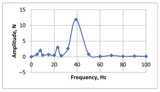
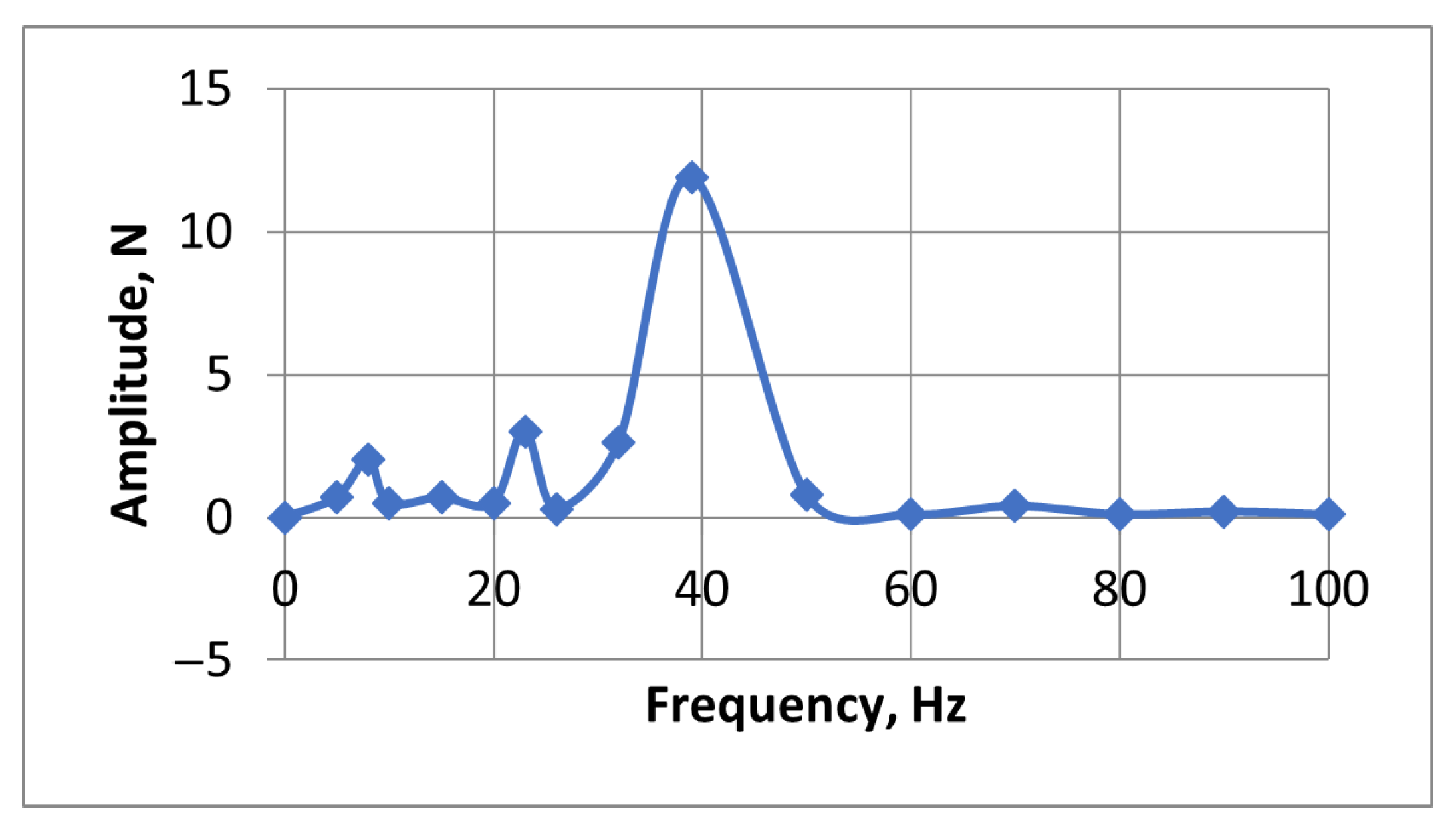
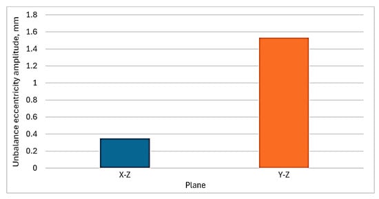
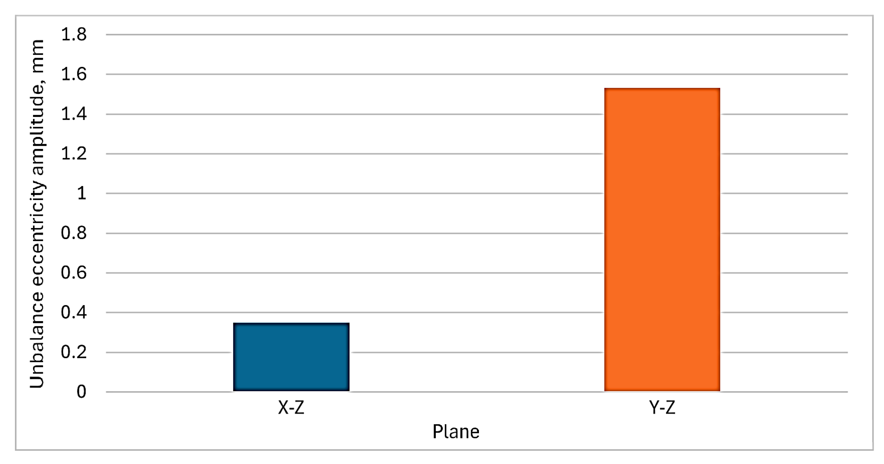
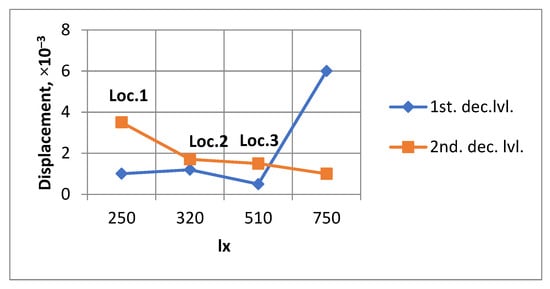
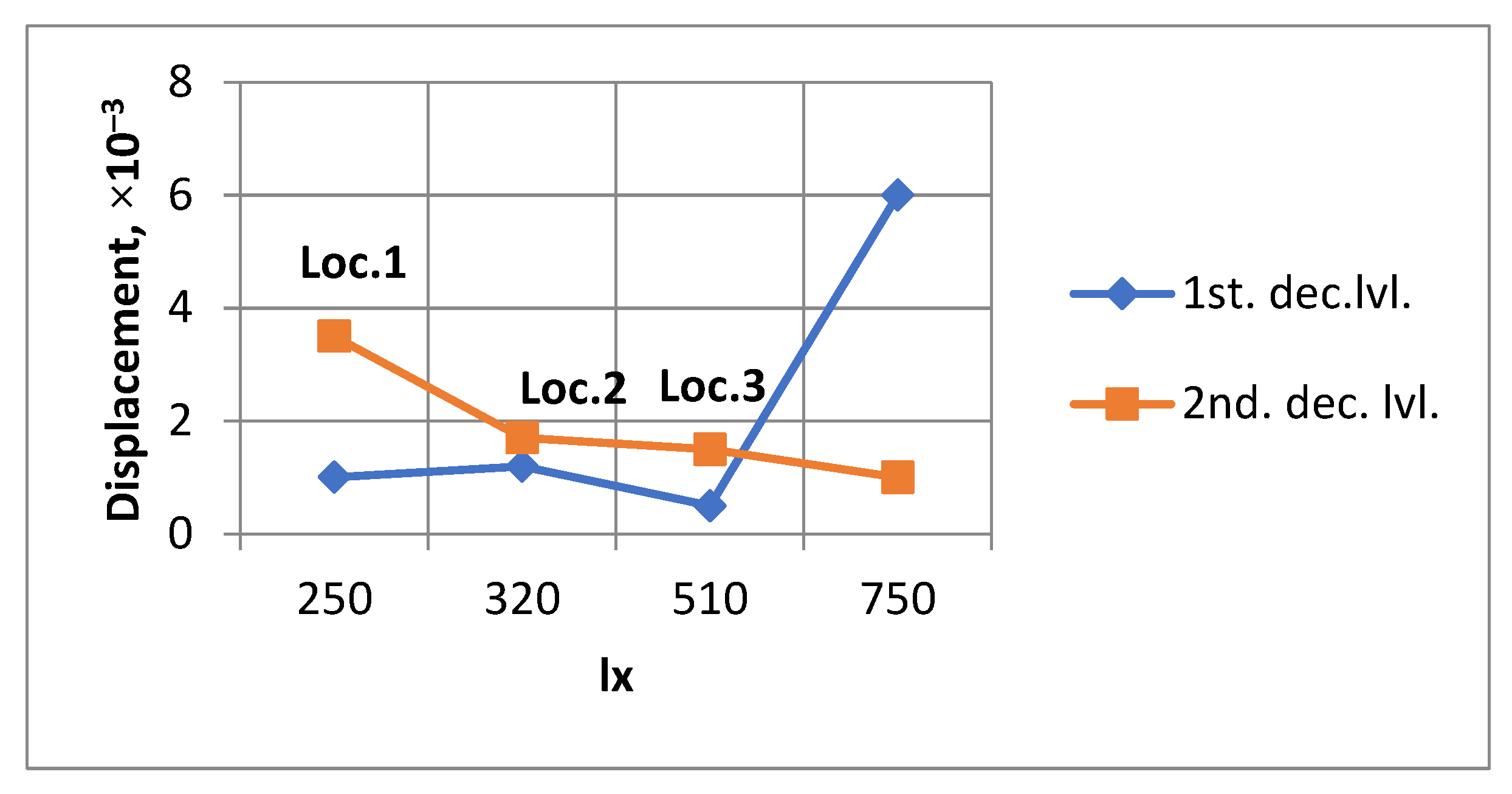
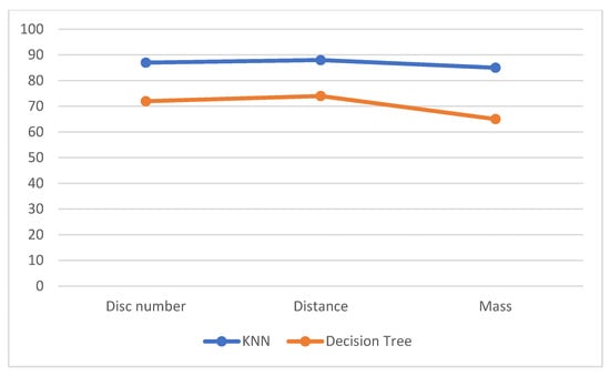
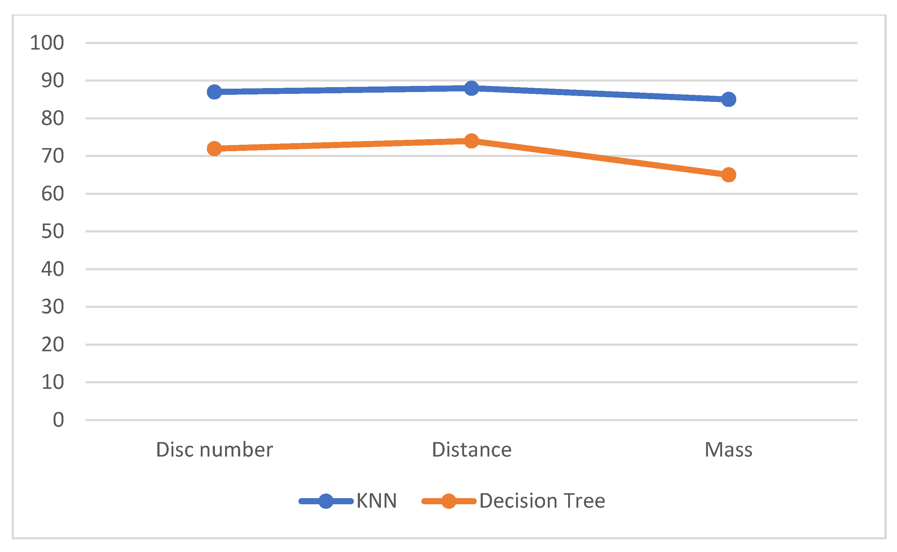
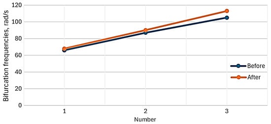
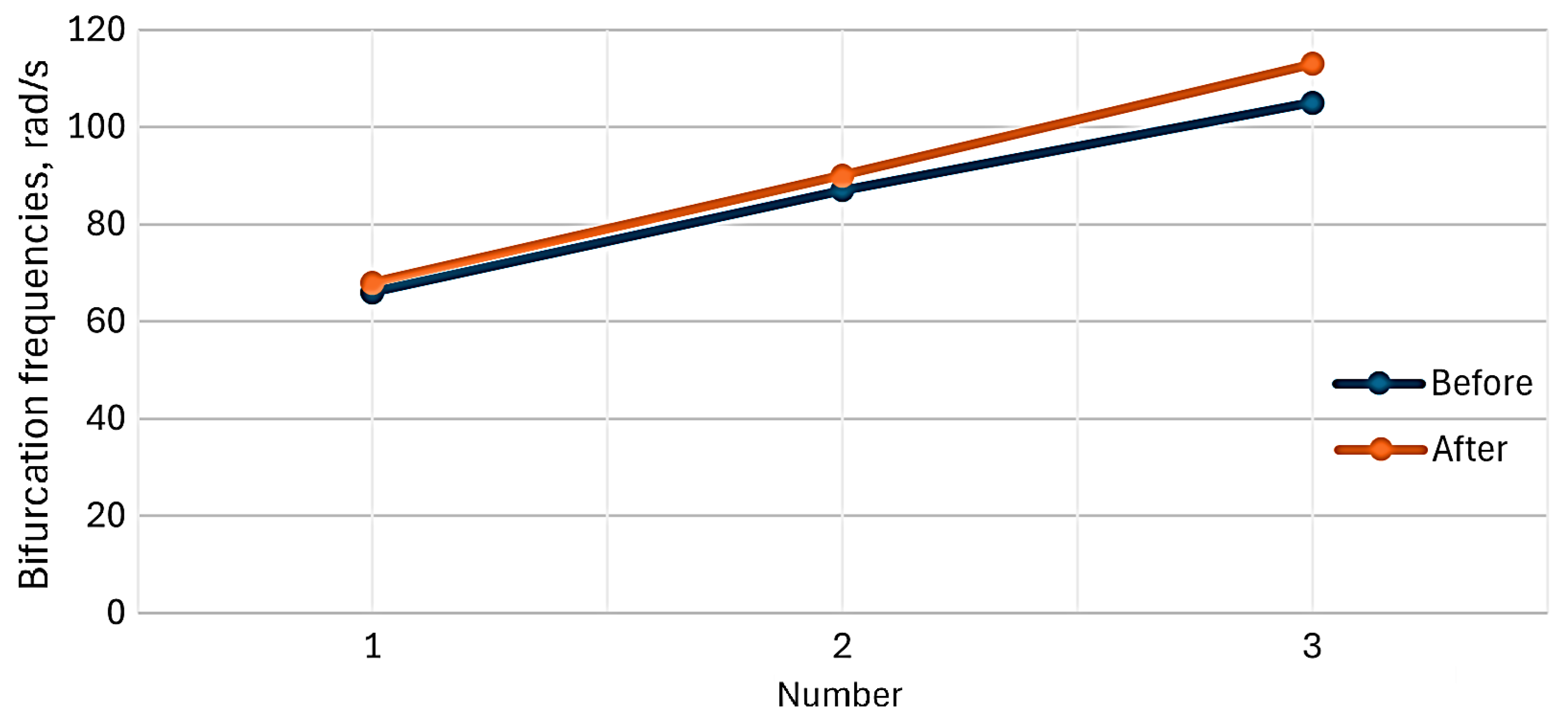
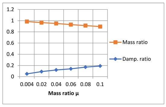
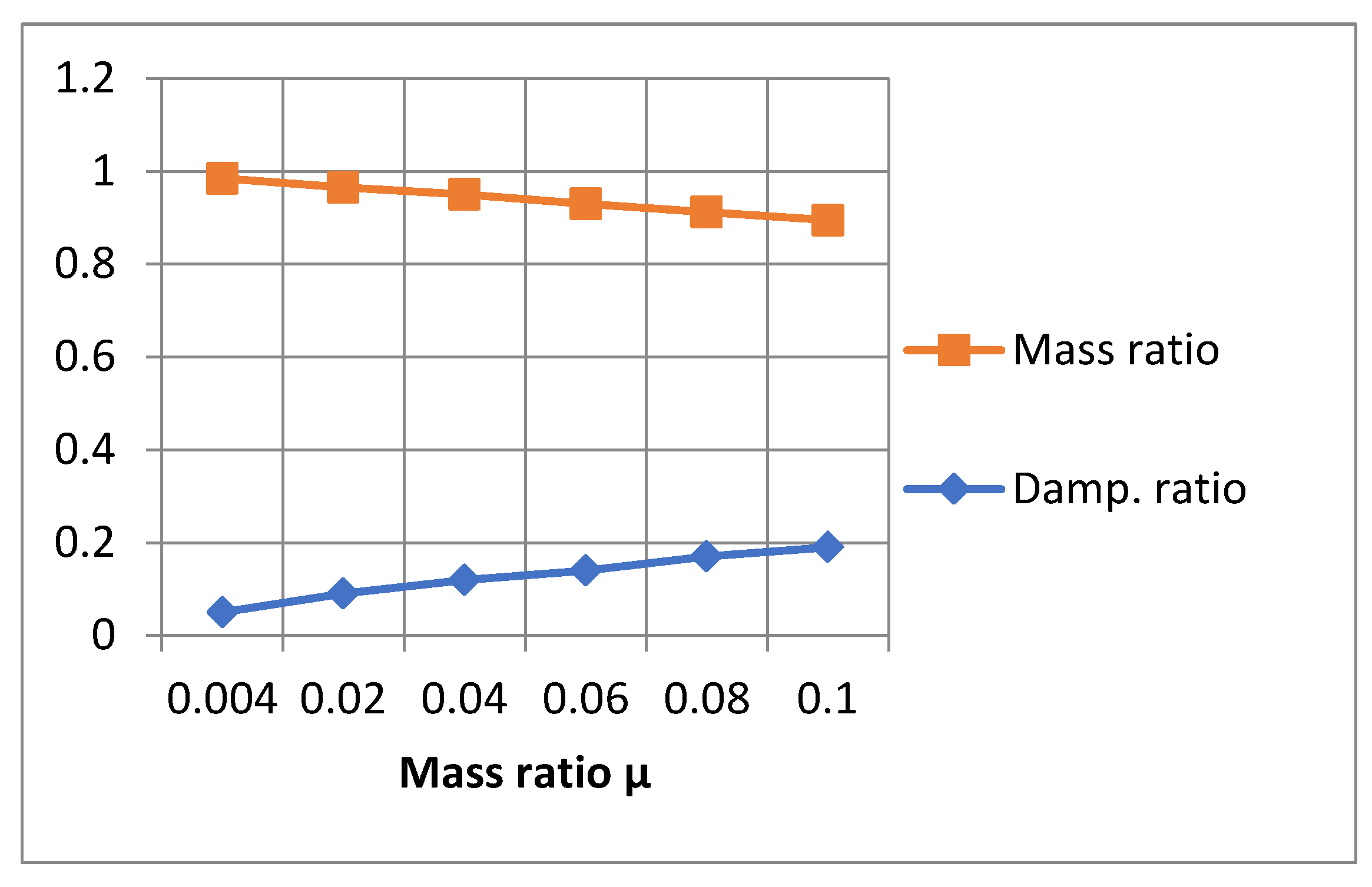
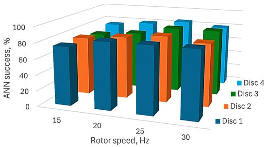
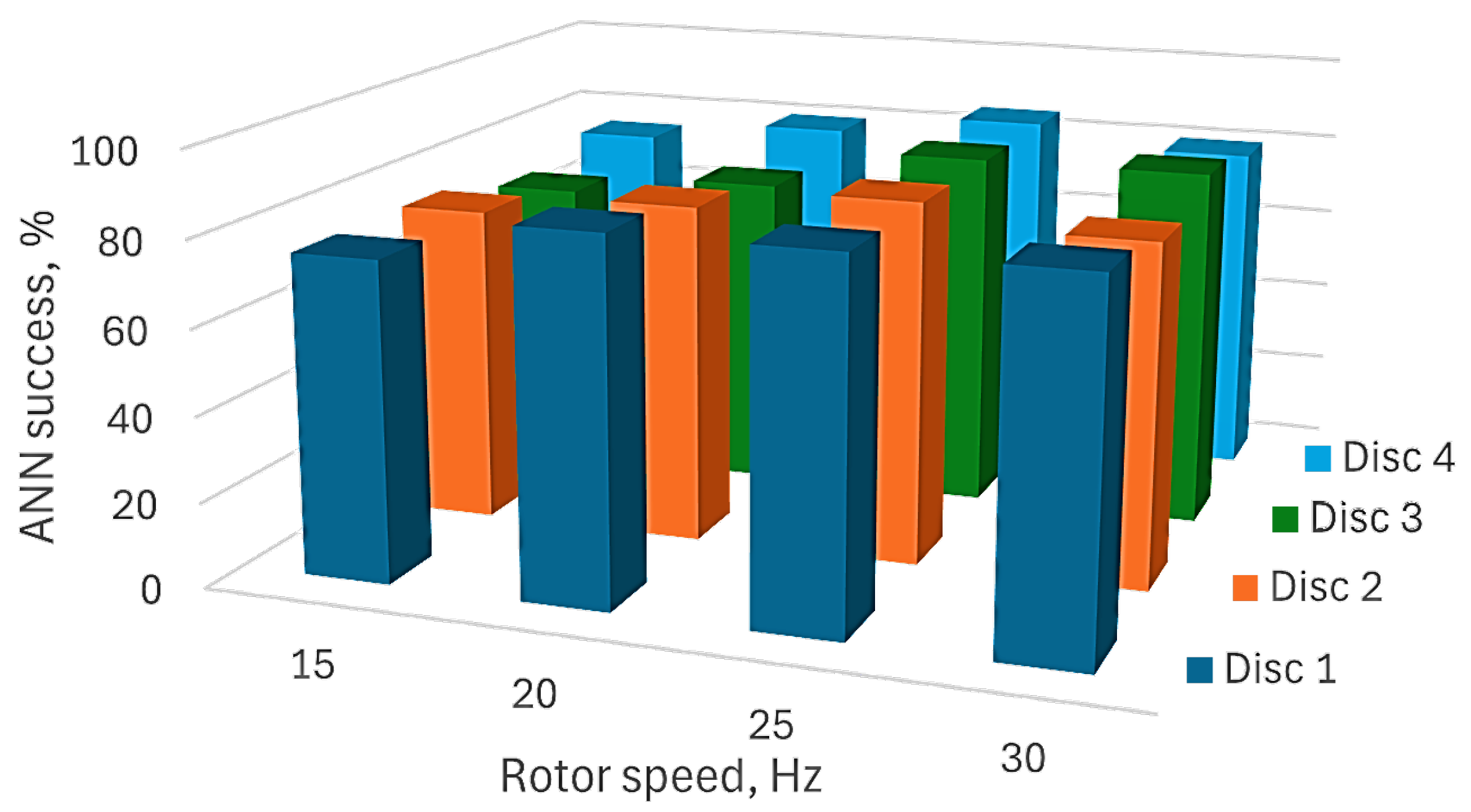
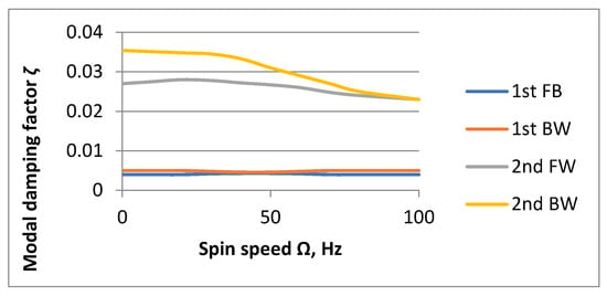
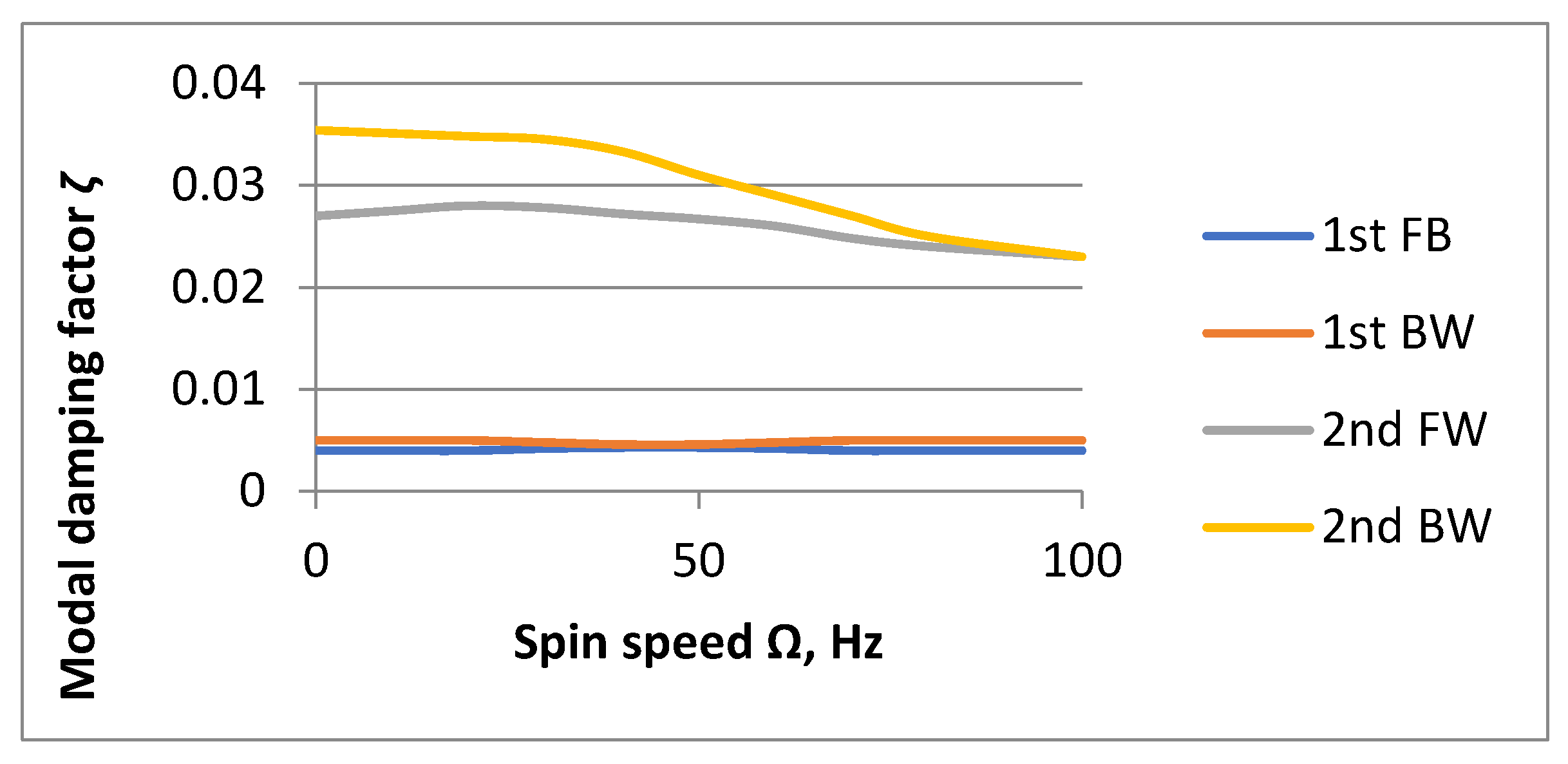
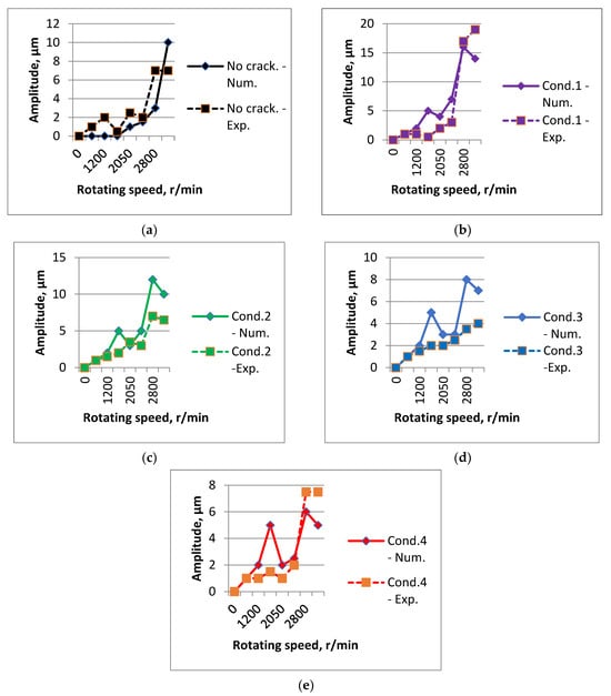
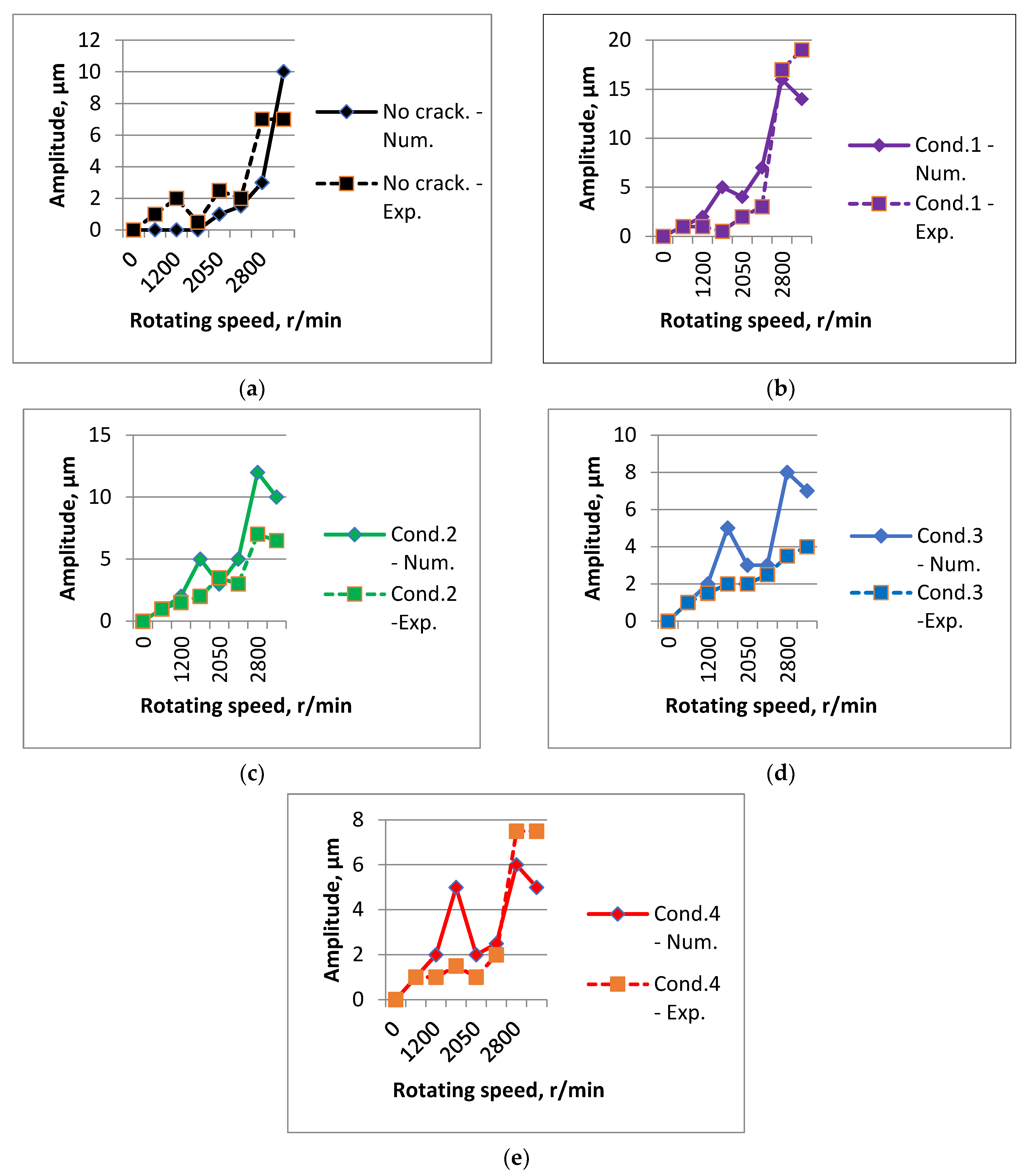
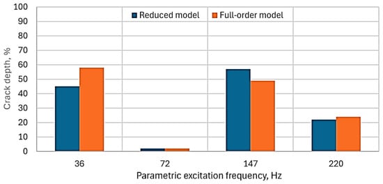
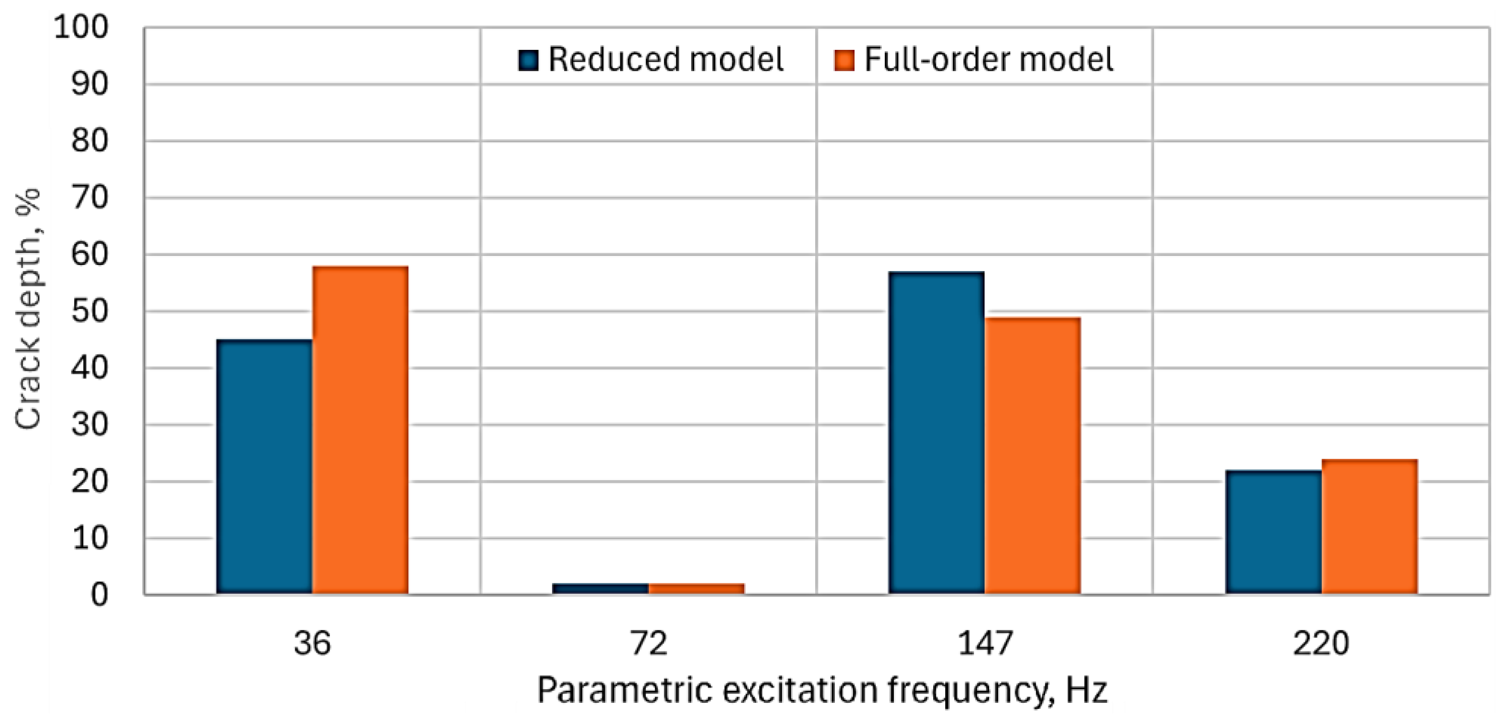
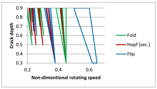
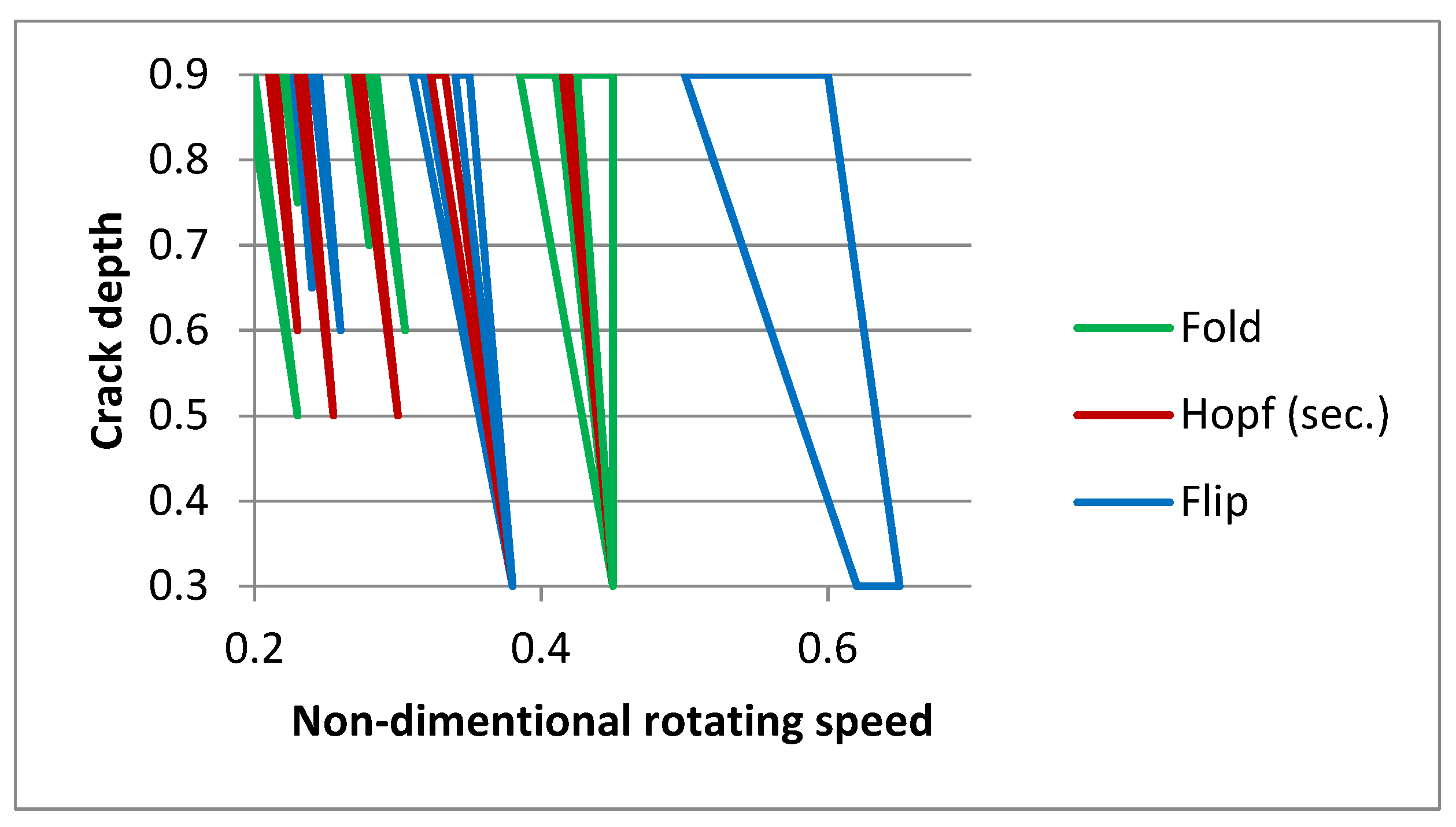
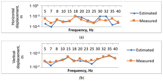
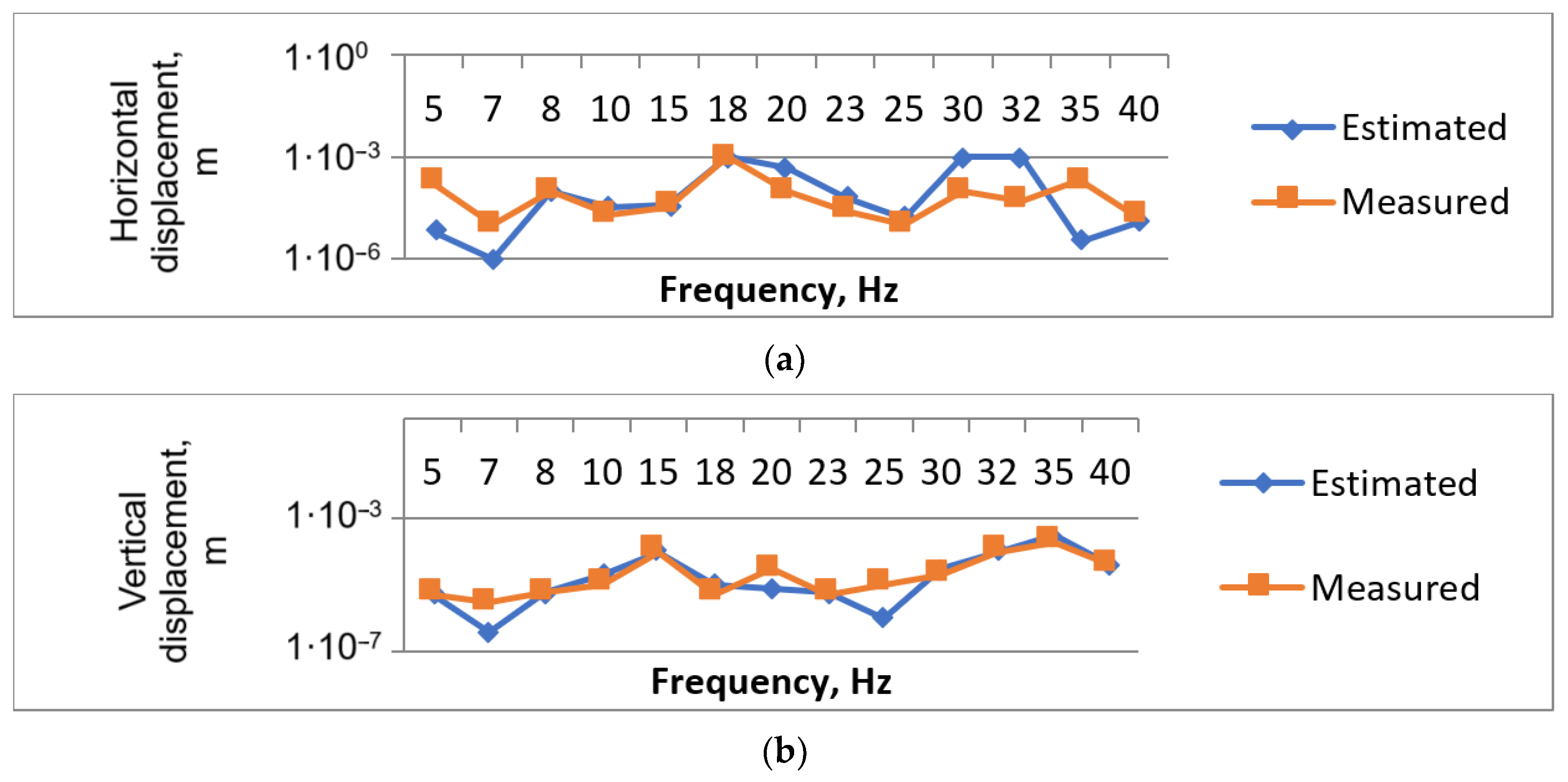
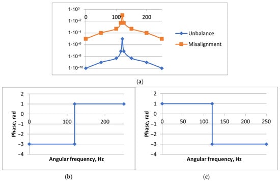
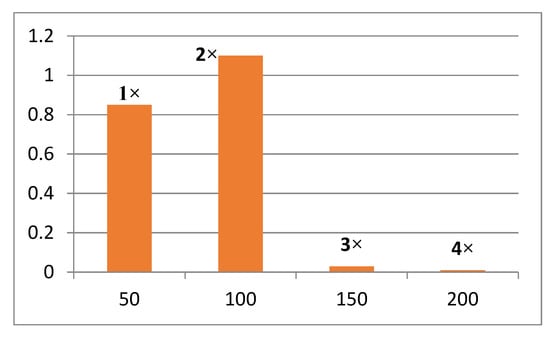
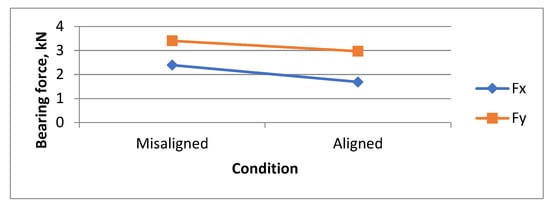
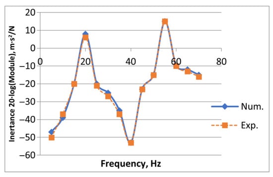
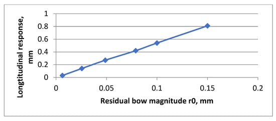
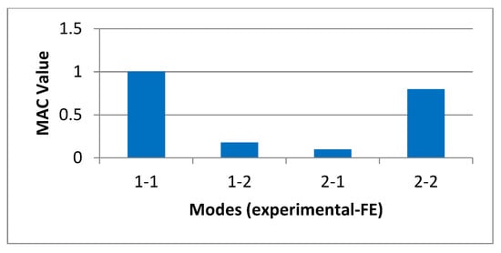
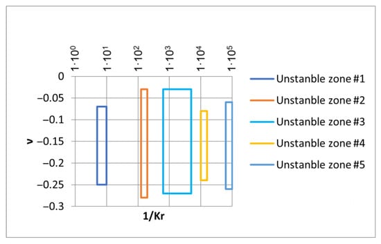
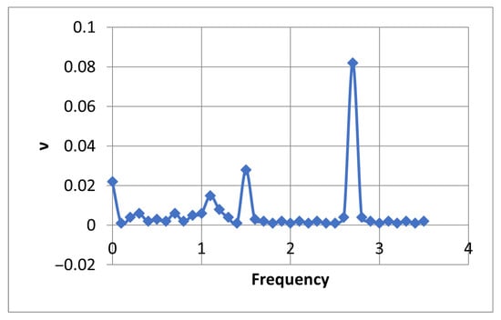
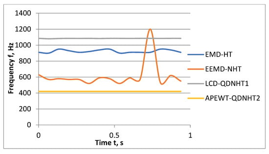
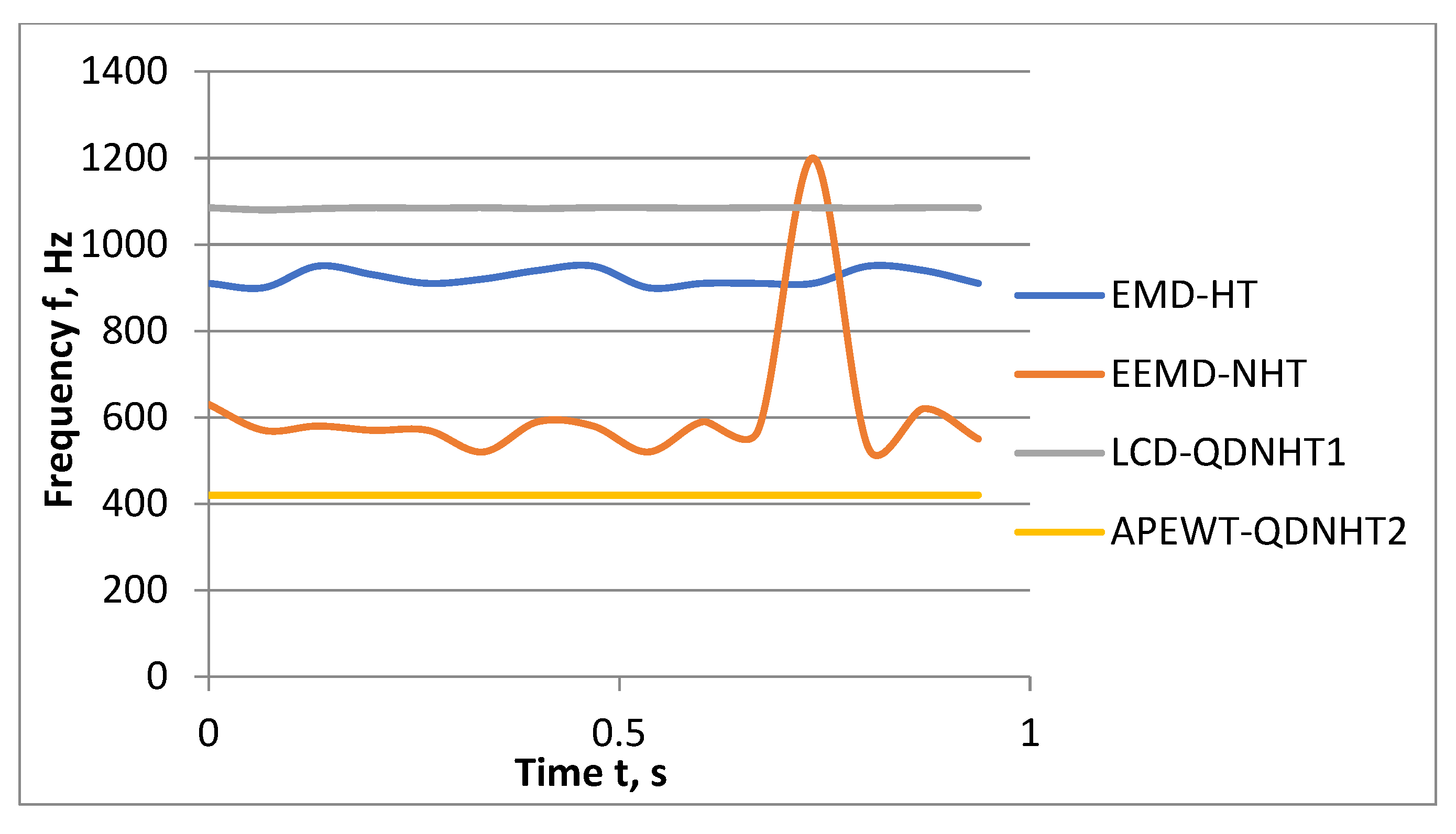
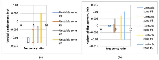
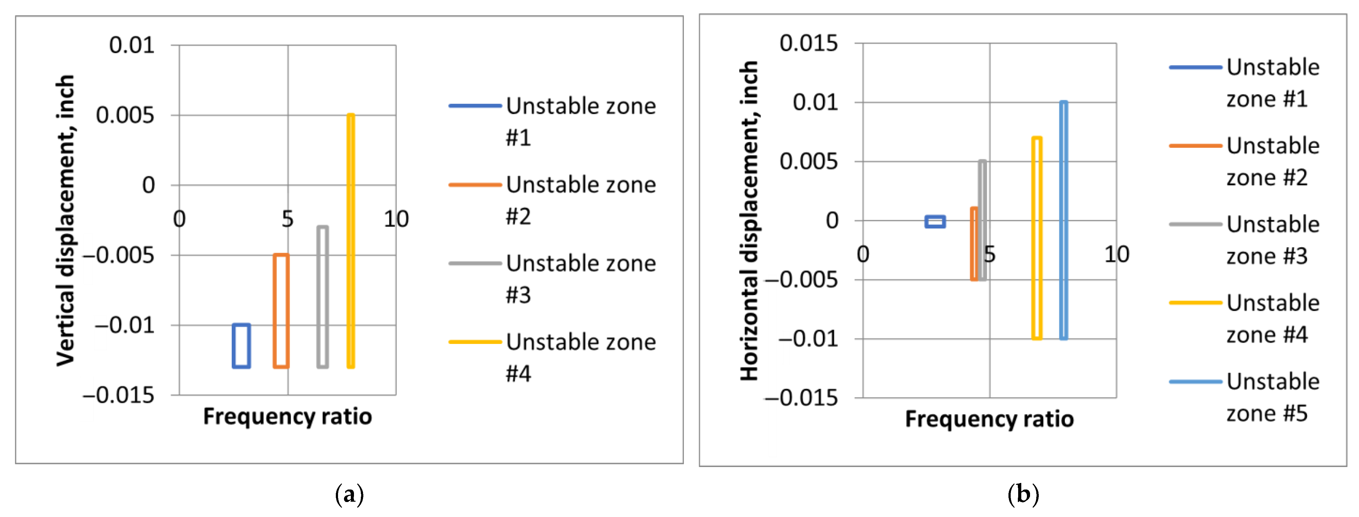
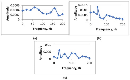
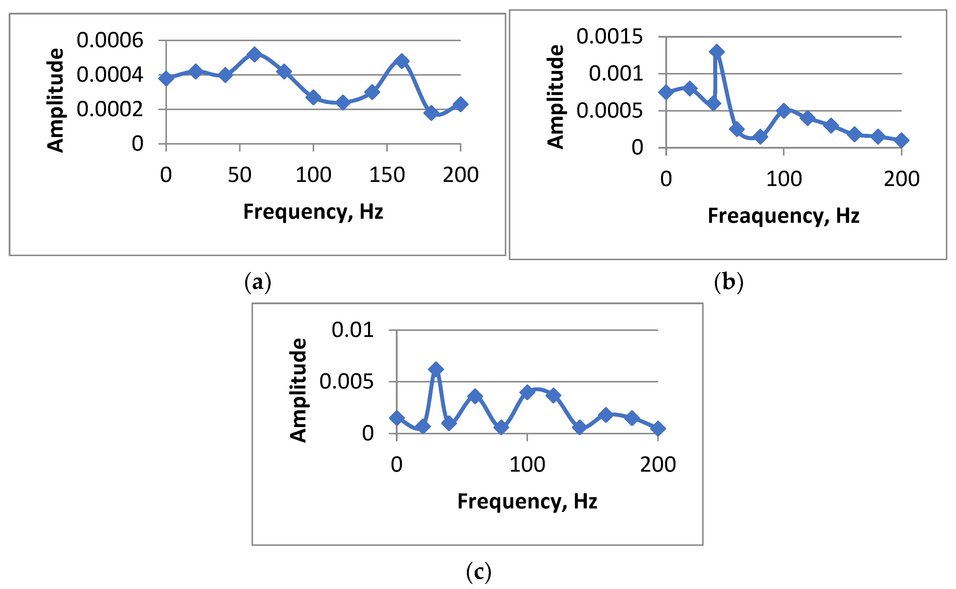
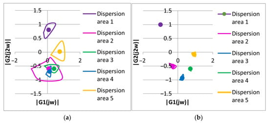
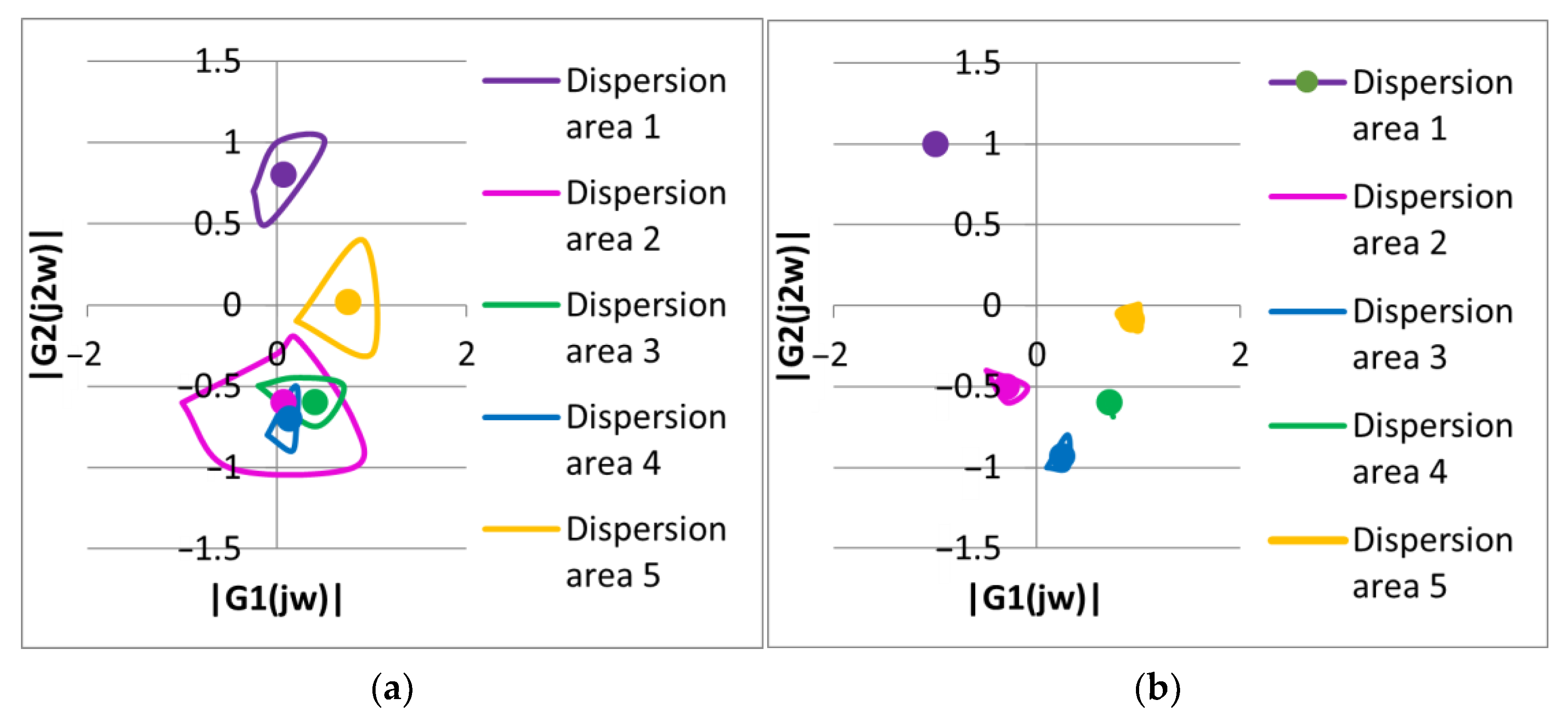
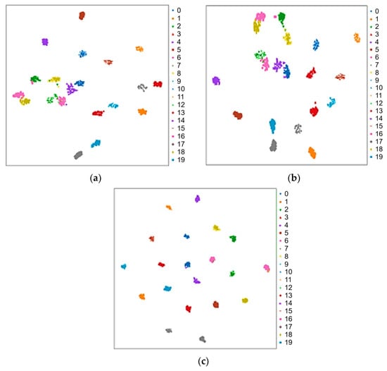
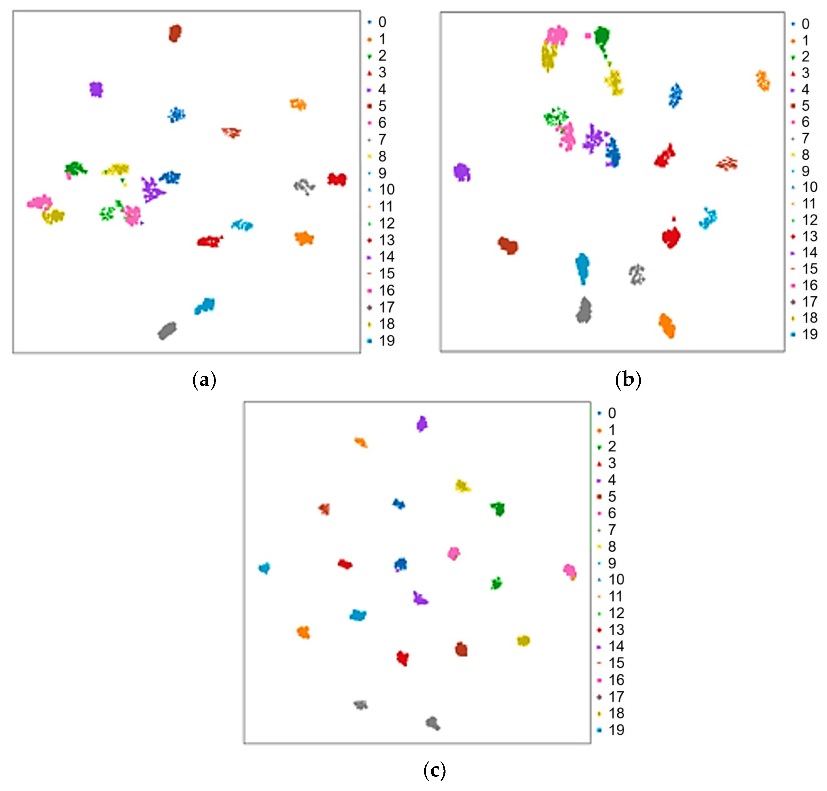
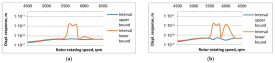
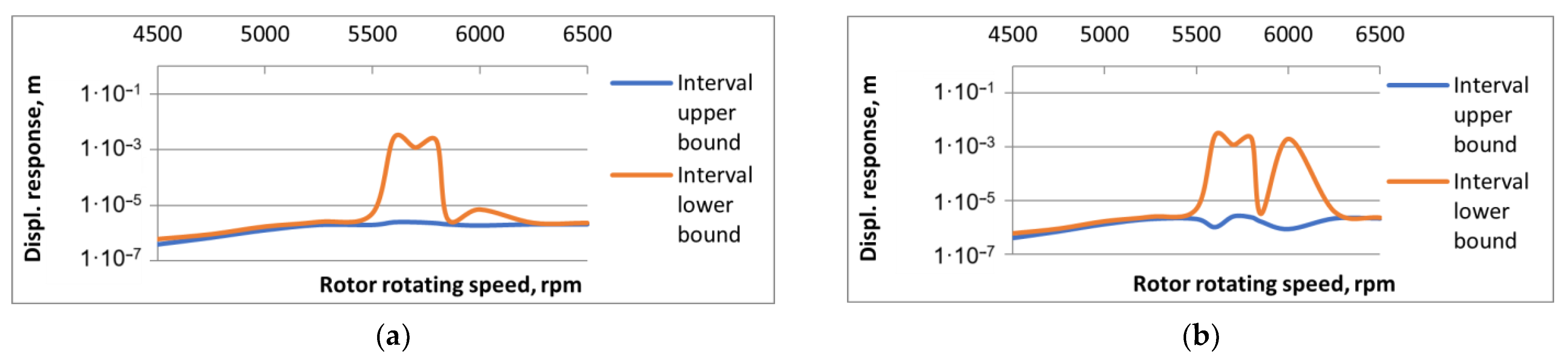
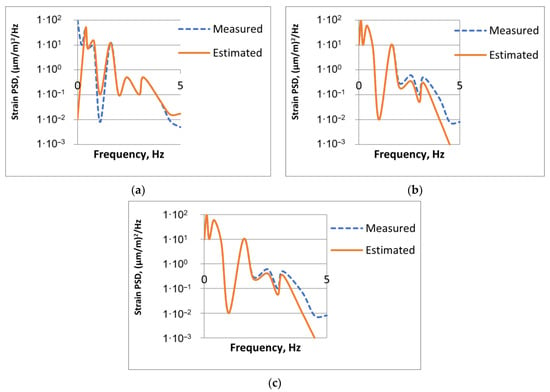
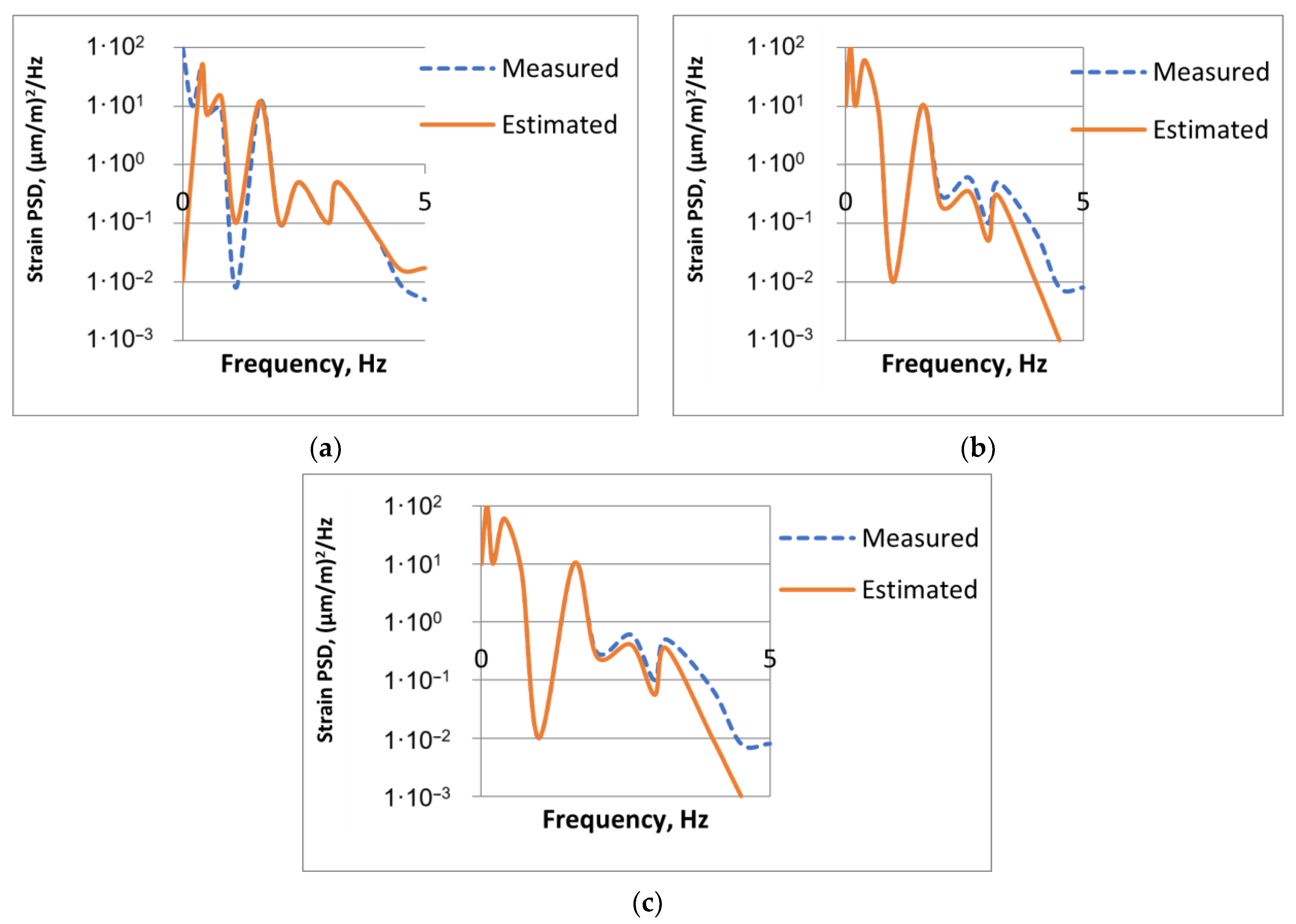
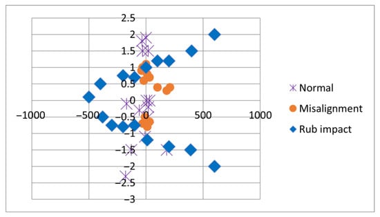
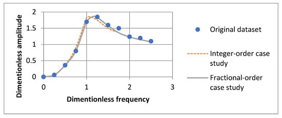
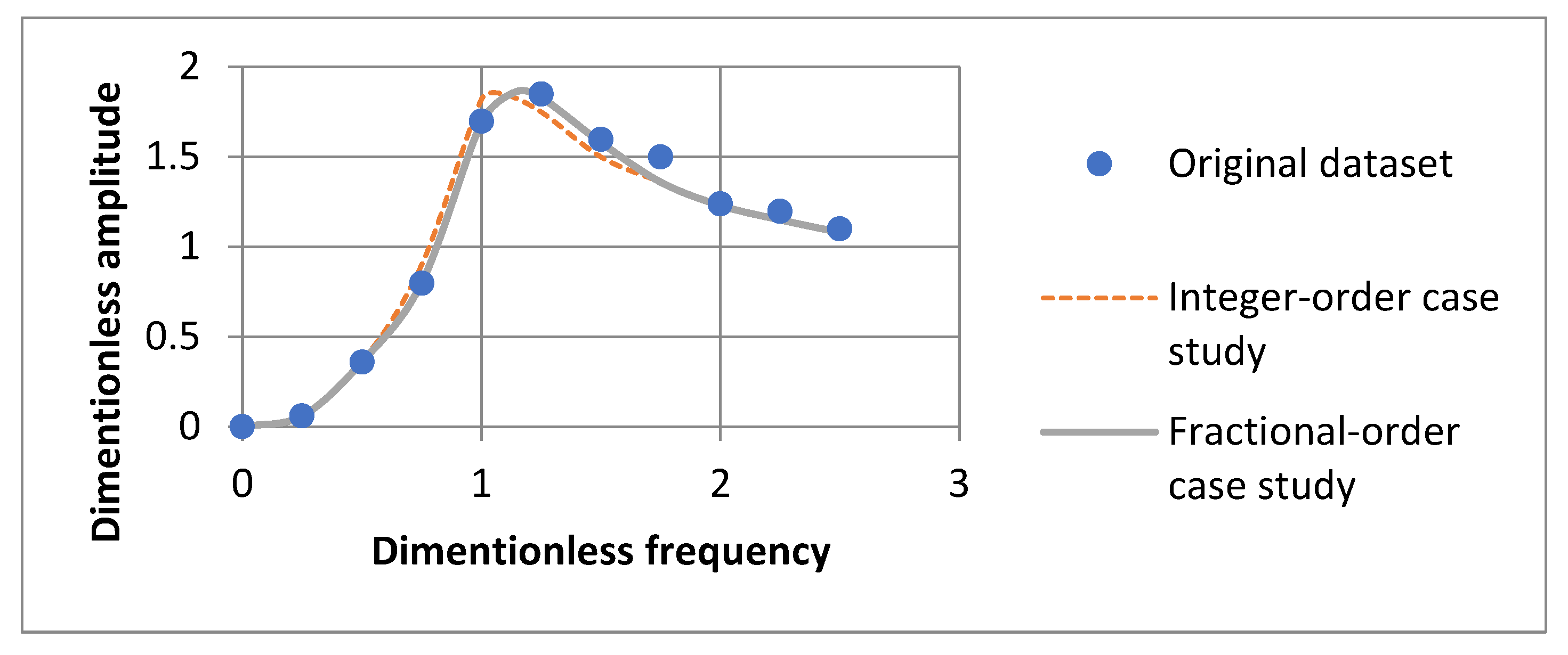
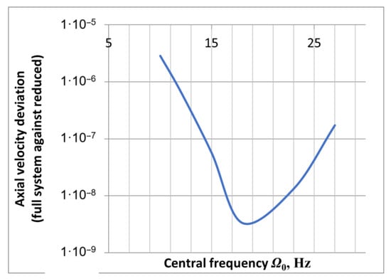
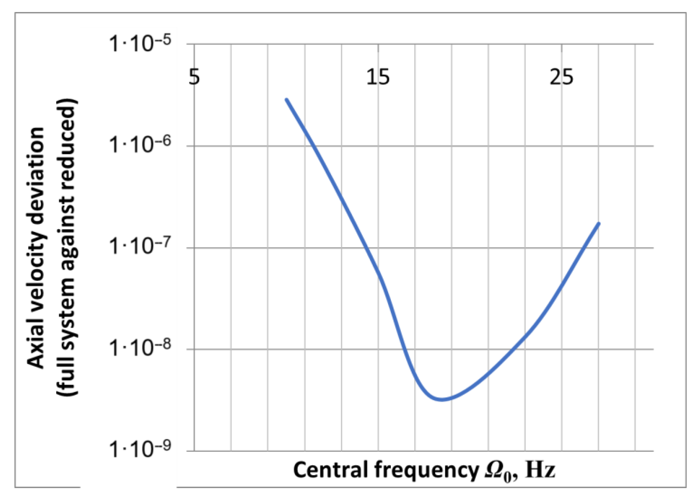
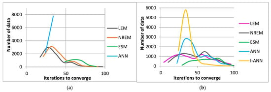
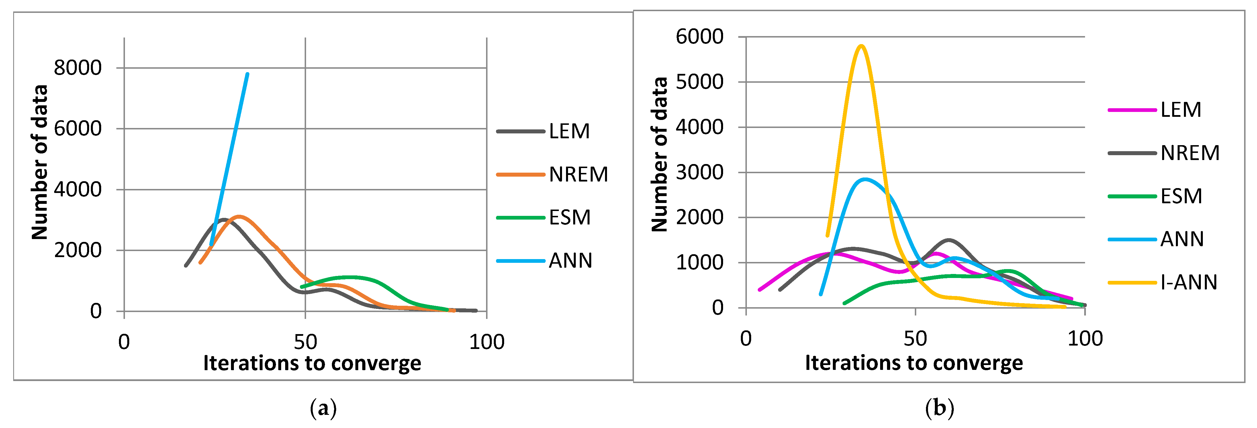
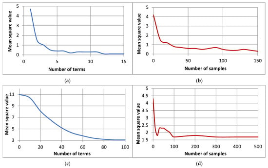
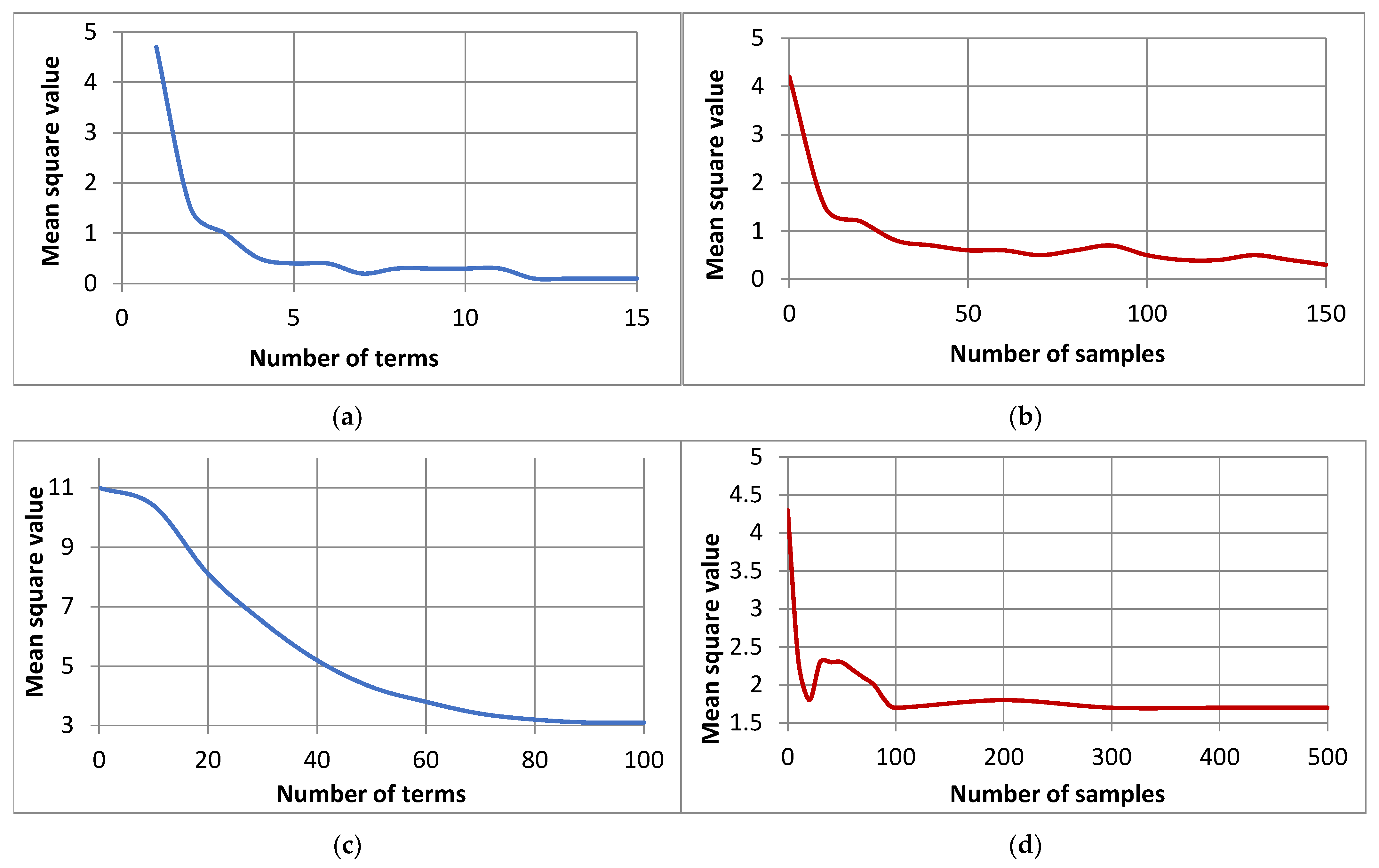
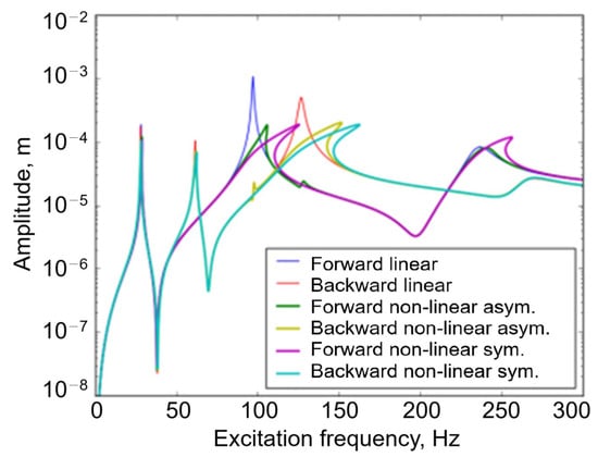
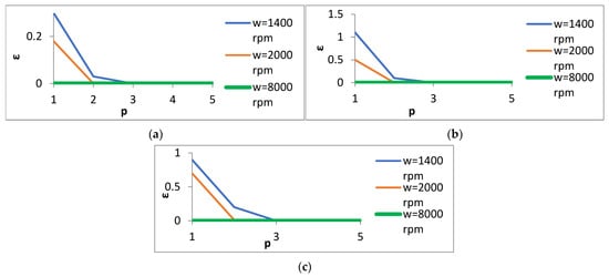
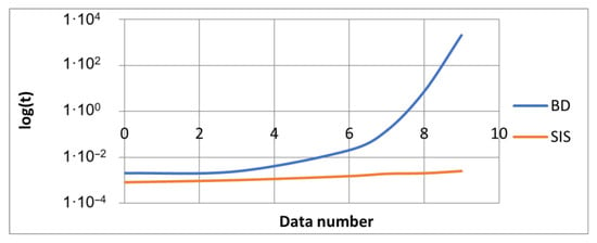
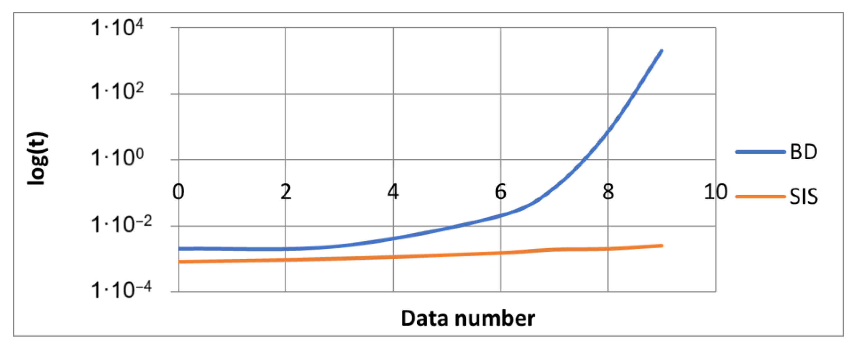
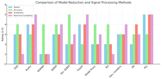
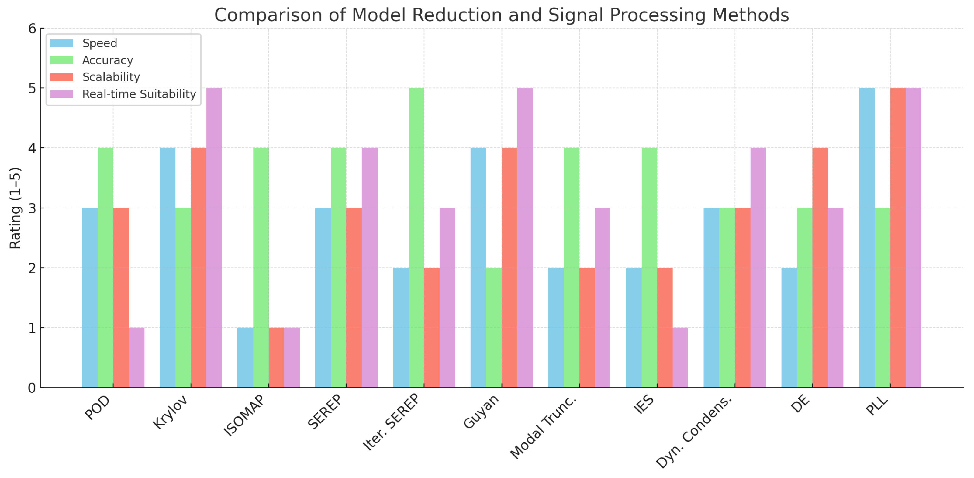
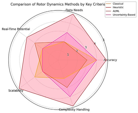
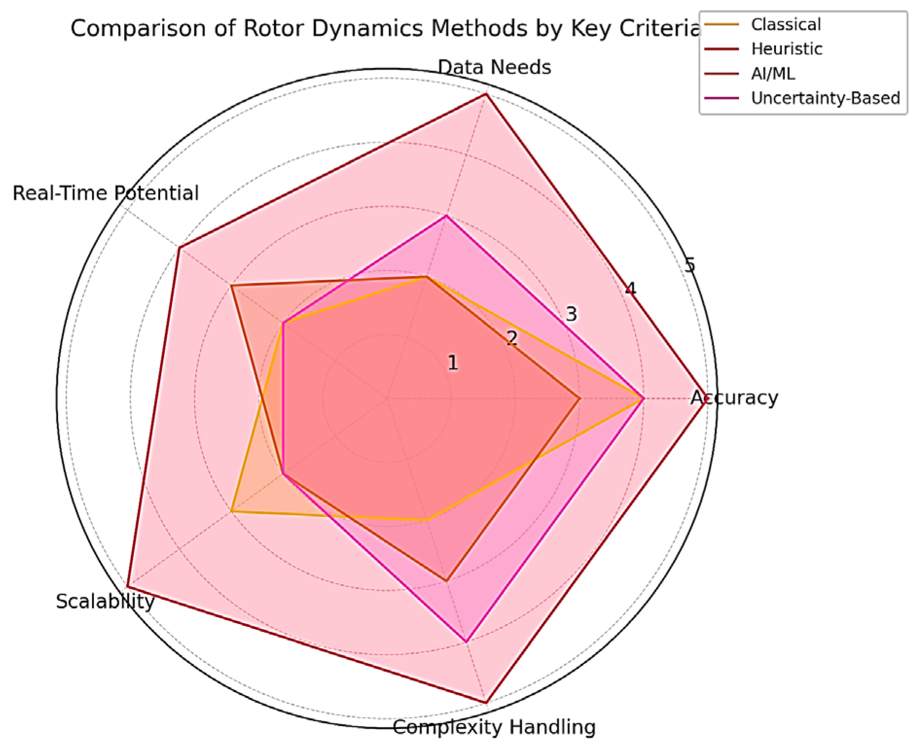

Disclaimer/Publisher’s Note: The statements, opinions and data contained in all publications are solely those of the individual author(s) and contributor(s) and not of MDPI and/or the editor(s). MDPI and/or the editor(s) disclaim responsibility for any injury to people or property resulting from any ideas, methods, instructions or products referred to in the content. |
© 2025 by the authors. Licensee MDPI, Basel, Switzerland. This article is an open access article distributed under the terms and conditions of the Creative Commons Attribution (CC BY) license (https://creativecommons.org/licenses/by/4.0/).