Performance Limits of VNIR Hyperspectral Imaging for Soil Heavy Metals in Camellia oleifera Plantations: A Strict Nested Cross-Validation Benchmark

Abstract

Visible–near-infrared (VNIR) hyperspectral imaging is promoted as a rapid substitute for ICP-MS in soil heavy metal monitoring, yet most evidence rests on single-split or non-nested validation. This study benchmarks VNIR prediction for Camellia oleifera plantation soils in Changshan County, Zhejiang, China (n = 83; 102 bands, approximately 401–1022 nm; 51 modeling indicators) under strict nested cross-validation, with all imputation, scaling, preprocessing, and model selection confined to each outer training fold. Four findings emerged. First, the highest observed mean ratio of performance to deviation (RPD) under the present protocol was 1.13. This did not reach the empirical 1.4 interpretive benchmark adopted here, and most fold-wise R² values were negative. Second, a 1D-CNN with squeeze-and-excitation attention performed significantly worse than a linear baseline for six of ten indicators and better for none; gains seen in the earlier non-nested exploratory analysis did not persist under leakage-controlled evaluation. Third, re-casting the task as regulatory risk level classification did not recover operational utility: Cr and Zn recall values were supported by only two and one exceeding samples, respectively, and cannot estimate population screening sensitivity. Fourth, an exploratory post hoc SHAP analysis using a full-data Random Forest assigned 24% of top wavelengths to Fe-oxide or organic-matter reference bands versus a 5.9% permutation null mean (empirical p = 0.020, the minimum attainable with 50 permutations). This attribution identifies plausible spectral proxy regions but is not independent evidence of predictive generalizability or causality. Separately, 22.9% of plots exceeded the GB 15618-2018 arsenic risk screening value. Within this dataset and validation design, VNIR imaging therefore supports neither reliable quantitative prediction nor operational screening.

1. Introduction

Camellia oleifera Abel. (oil-tea camellia) is one of the most economically important woody oil tree species in southern China, with cultivation concentrated in Hunan, Jiangxi, and Zhejiang provinces and a national plantation area exceeding 4 million ha [1,2]. Quzhou City and its Changshan County, located in western Zhejiang Province, are designated geographic indication production zones for high-quality oil-tea. Because plantation yield, oil quality, and food safety depend strongly on subtropical red soil fertility and chemistry [3,4,5], baseline characterization of soil physicochemical and heavy metal status across plantation plots is a fundamental requirement for precision soil management.

The subtropical red soil weathering environment of southeastern China combines naturally low pH (typically 4.0–6.0) with elevated free iron oxide content, conditions that markedly increase the bioavailability and plant uptake potential of heavy metals such as Pb, As, Cd, and Hg [6,7,8,9]. Recent evidence further documents heavy metal accumulation in Camellia agroecosystems and Cd transfer through the soil–leaf–infusion continuum [10]. Conventional ICP-MS quantification, although accurate, is destructive, slow, and impractical at the plot scale. Visible–near-infrared (VNIR, ~400–1000 nm) hyperspectral reflectance spectroscopy has consequently been advanced as a rapid, non-destructive complement [11,12,13,14,15,16].

The mechanistic basis for VNIR sensing of heavy metals is well established but indirect. Iron oxide-related electronic transitions produce characteristic absorption near 440 nm, 530 nm, and 870 nm [17]; soil organic matter suppresses overall reflectance in the 550–770 nm region [11,18]; clay minerals contribute primarily beyond 1400 nm in the SWIR region. Direct spectral signatures of Cd, Pb, As, and Hg are essentially absent in VNIR, so prediction must proceed indirectly through co-variation with iron oxides, organic matter, and pH [19,20,21,22].

Although recent deep learning architectures—1D-CNN with attention [23,24], Transformer–CNN hybrids [25,26,27], and channel attention CNN-LSTM models [28,29,30]—and multi-task learning frameworks [31,32,33,34] have shown promise on large public datasets such as LUCAS (n > 20,000) [35,36,37], three persistent gaps limit translation to plantation-scale management. First, the actual performance of these methods on small (n < 100), single-region, low-variability datasets—the realistic situation for plot-scale agronomic monitoring—has not been rigorously characterized, because most reports use single-split or non-nested cross-validation protocols that risk inflating estimates through preprocessing and model-selection bias. Second, regression-style metrics (R², RMSE, RPD) optimize for precise concentration prediction, but on small-sample subtropical red soils where the spectrum has limited intrinsic dimensionality, the conventional RPD > 2.0 target may be physically unattainable, and the literature contains few rigorous evaluations of when VNIR fails. Third, the practical end-use of soil hyperspectral imaging in plantation management is risk-level screening—whether a plot is safe, marginal, or contaminated—rather than precise concentration prediction, yet classification-based formulations remain rare [38].

Accordingly, this study provides (1) a strict nested cross-validation benchmark across 10 focus soil indicators, with all imputation, preprocessing, and model selection performed within each outer training fold, reporting the highest observed mean RPD under the present protocol rather than an attainable limit; (2) a head-to-head comparison of 1D-CNN-SE deep learning against traditional baselines under the strict protocol, with paired bootstrap confidence intervals on ΔRPD; (3) a comparison of five wavelength selection algorithms (CARS [39], SPA, UVE, Random Frog, RF-Importance); (4) reformulation of ten heavy metals as a risk-level classification problem using per-sample pH-stratified GB 15618-2018 thresholds [40], with class support, balanced accuracy, and high-risk recall reported alongside accuracy; and (5) exploratory post hoc SHAP attribution [41,42] cross-checked against a permutation null distribution. The central contribution is methodological rather than predictive: rather than claiming high accuracy, this study documents the observed performance under a leakage-controlled fitted pipeline, identifies remaining conditionality from dataset-level target selection and random non-spatial folds, and evaluates whether attribution patterns align with plausible soil spectral proxy regions. The conclusions are restricted to this sample, spectral range, and validation design.

2. Materials and Methods

2.1. Study Area and Soil Sampling

The study was conducted in mature C. oleifera plantations in Changshan County, Quzhou City, Zhejiang Province, China (approximately 28.9° N, 118.5° E). The region experiences a subtropical monsoon climate with a mean annual temperature of approximately 17 °C and annual precipitation of 1700 mm. Regional descriptions identify the area broadly as subtropical red soil terrain; plot-specific soil taxonomic classes, cation exchange capacity, texture, and mineralogical or Fe-oxide composition were not measured in this survey [8,9]. Eighty-three soil samples were collected from the surface mineral soil interval (0–20 cm), selected for topsoil monitoring and surface contamination assessment using a stratified random scheme spanning representative plantation plots across the county’s principal oil-tea production townships [43]. Each sample was a composite of three sub-samples taken within a 1 m radius. After field collection, samples were air-dried, mechanically ground, sieved through a 2 mm mesh, and homogenized; a subsample of each was further ground to pass a 0.149 mm (100-mesh) sieve for hyperspectral measurement and chemical analysis.

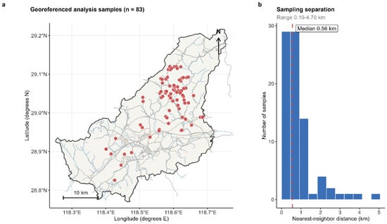
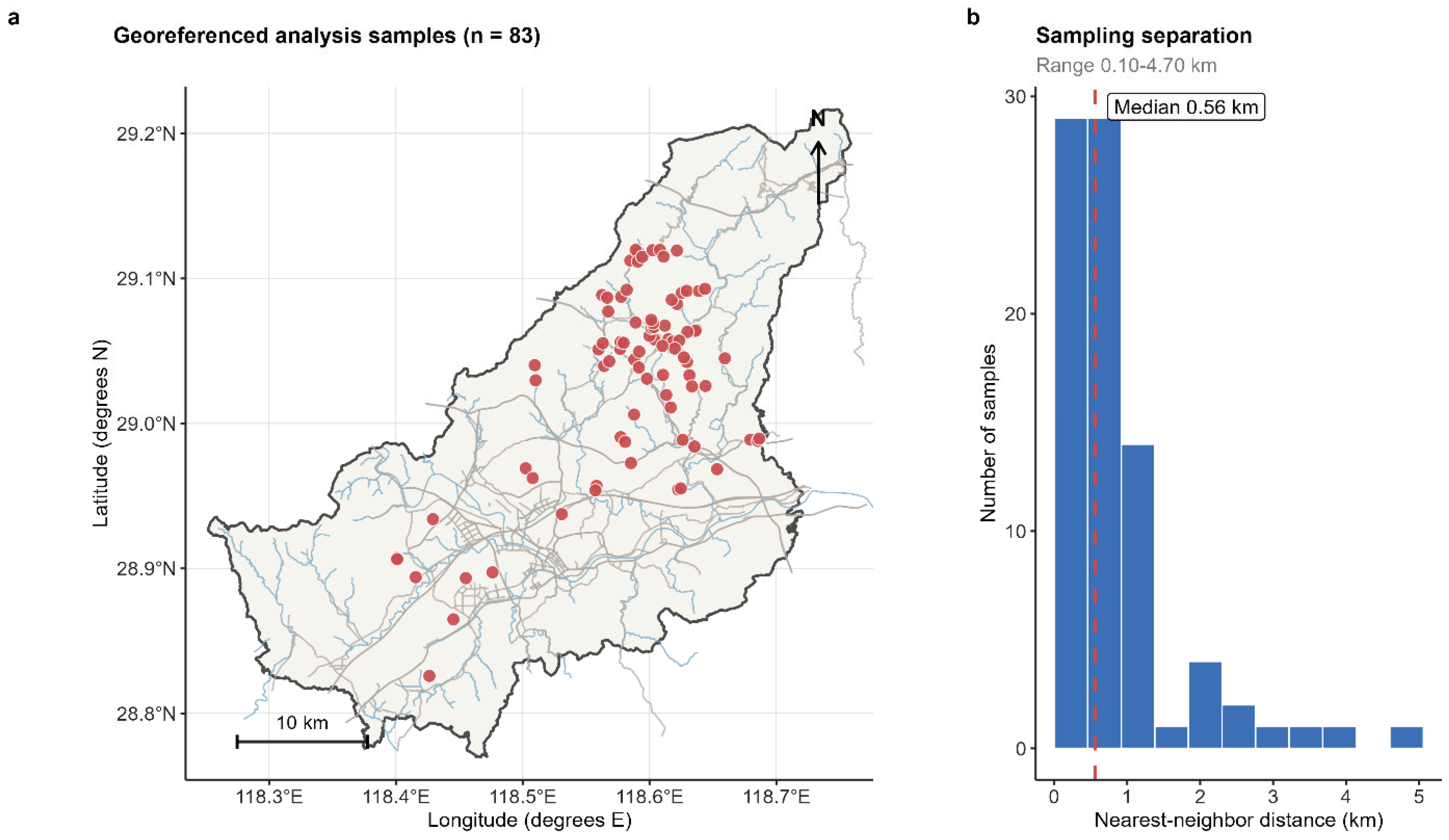
All 83 analysis samples were georeferenced with a handheld GNSS receiver (eTrex 22x, Garmin International Inc., Olathe, KS, USA) within the Changshan County boundary, spanning 118.40085–118.68651° E and 28.82585–29.11965° N (Figure 1a). Nearest neighbor distances ranged from 0.10 to 4.70 km (median 0.56 km; Figure 1b). Measured soils were acidic (pH 4.39–6.18; mean 5.12), with bulk density of 1.35–1.58 g/cm³ (mean 1.46) and SOM of 8.19–92.5 g/kg (mean 29.8).

Figure 1. Spatial distribution and spacing of the 83 analysis samples in Changshan County. (a) Georeferenced sampling locations within the county boundary; roads and waterways are shown for orientation. (b) Distribution of nearest neighbor distances calculated after projection to UTM Zone 50N (range 0.10–4.70 km; median 0.56 km). The nested cross-validation used random folds rather than spatial blocks; the map documents, but does not eliminate, potential spatial dependence.

Sampling was conducted during April–May 2026 over three field trips. The sampled Camellia oleifera plantations were 8 years old and received routine oil-tea plantation management, including regular fertilization, liming, and plant protection practices. All 83 analysis samples were georeferenced within Changshan County, Zhejiang, China (118.40085–118.68651° E; 28.82585–29.11965° N). For geographic context, 30 m ASTER DEM extraction gave approximate elevations of 94–390 m (mean 178.9 m; median 159.0 m) and slope estimates of 0.7–33.7° (mean 12.7°; median 13.2°). A generalized Macrostrat layer places the sampled area within a broad Paleozoic sedimentary rock domain; this regional map does not resolve plot-scale lithology. The geographic strata were the principal oil-tea production townships. Point-in-polygon assignment gave 30 samples in Fangcun, 24 in Xinchang, 8 in Daqiaotou, 6 in Dongan, 4 each in Tonggong and Huibu, 3 in Zigang, 2 in Jinchuan, and 1 each in Baishi and Hejia. At each plot, three subsamples were collected from representative under-canopy and inter-row positions within a 1 m radius and composited.

Before sampling, surface organic litter was removed without disturbing the mineral soil. The 0–20 cm surface mineral soil samples were air-dried for 48 h, stored at room temperature before analysis, mechanically ground, passed through a 2 mm sieve, homogenized, and further ground to 0.149 mm (100 mesh). Between samples, the grinder and contact surfaces were emptied, brushed, and wiped with clean laboratory tissue; a small purge portion was discarded before the analytical fraction was collected. These steps were used to minimize carry-over.

2.2. Reference Chemical Analysis and Quality Assurance

Fifty-four reference soil indicators were quantified in certified laboratories (China National Accreditation Service for Conformity Assessment, CNAS-accredited). Soil pH (1:2.5 soil/water suspension) was measured potentiometrically; bulk density (BD) was determined gravimetrically on undisturbed cutting ring cores; soil organic matter (SOM) followed the Walkley–Black potassium dichromate method; total nitrogen (TN), total phosphorus (TP), available phosphorus (AP), available potassium (AK), and hydrolyzable nitrogen (HN) followed Chinese national agricultural standards. Forty-six elemental indicators were quantified by inductively coupled plasma–mass spectrometry (ICP-MS; Agilent 7900, Agilent Technologies, Santa Clara, CA, USA) following microwave-assisted acid digestion (HF–HClO₄–HNO₃ for total digestion or aqua regia for partial digestion as appropriate). Quality assurance and quality control procedures included one method blank, one duplicate sample, and one certified reference material (GBW07404 yellow-red soil) per batch of 20 samples; recoveries for Pb, Cd, As, Cr, Cu, Zn, Ni, and Hg fell within 90–110% of certified values, and analytical relative standard deviations were below 5% for all elements. Detection limits were 0.1 mg/kg for Cd and 0.5 mg/kg for As and Pb. All elemental concentrations, including total Hg, are reported throughout in mg/kg, matching the units in the source analytical workbook and the GB 15618-2018 risk screening values used in Section 2.7.

The ICP-MS was calibrated with traceable multi-element working standards prepared from certified stock solutions covering the expected concentration range. Sc, Ge, Rh, In, and Bi were used as internal-standard elements to monitor signal drift and matrix effects. The retained QA/QC records identify one method blank, one duplicate sample, and one certified reference material (GBW07404 yellow-red soil) per batch of 20 samples.

2.3. Hyperspectral Data Acquisition

Reflectance spectra (approximately 401–1022 nm, 102 bands at ~6 nm spectral sampling) were acquired in a darkroom using a laboratory hyperspectral imaging system (SCI-VN100G, Westlake Intelligent Vision Technology (Hangzhou) Co., Ltd., Hangzhou, China). Spectral cubes were calibrated against a 50% reflectance Spectralon-equivalent white reference and a dark current reference using the standard formula R = (DN_sample − DN_dark)/(DN_white − DN_dark) × 0.5, where the factor 0.5 corrects for the 50% nominal reflectance of the white reference. For each sample, a region of interest of approximately 1500 ± 200 pixels was delineated on the soil surface using a uniformity threshold (intra-ROI brightness CV < 5%); individual pixel spectra were screened (Pearson correlation with the per-sample median > 0.98 and adjacent-band-jump < 0.05), and the remaining valid pixels (mean 1380 per sample, range 1100–1820) were averaged to yield one mean reflectance spectrum per sample. Three samples that initially yielded radiance-like spectra were corrected via re-application of the white reference normalization and retained after confirming that the corrected spectra fell within the population envelope. Retained model outputs store integer-rounded band labels, including 1022 nm for the upper-edge band. The original unrounded wavelength vector was not available in the retained study records, so no finer endpoint precision is claimed.

2.4. Quality Screening, Imputation, and Transformation

Indicator-level quality screening removed three of the 54 indicators: pH (CV = 6.8%, variability too low for spectral inversion under such homogeneity), BD (CV = 4.6%, same reason), and Au (42% values below detection limit). For the 51 retained indicators, samples with values reported as zero (interpreted as below-detection-limit) and samples with explicitly missing values (Tb 9.6%, Yb 9.6%, Rh 14.5%, Hg 4.8%) were jointly imputed using iterative imputation with Bayesian ridge regression as the per-feature predictor (sklearn IterativeImputer, max_iter = 10, tolerance = 0.001), exploiting the strong inter-correlation among rare earth elements and trace metals. Within the strict nested cross-validation protocol (Section 2.7), the imputer was refit on every outer training fold and applied to the corresponding outer test fold to prevent target leakage. Forty indicators with absolute skewness > 1 (most heavy metals and rare-earth elements) were log10-transformed (with an offset for zero-imputed entries) prior to modeling; all performance metrics were computed on the log-transformed scale at which the models were fitted (Section 2.9). The choice of log10 transformation was applied to the response (target) variable only; the spectral matrix was not log-transformed.

The CV < 10% criterion was a pragmatic, study-specific prescreening rule adopted before modeling to flag near-constant indicators in this small dataset. It was intended to identify response variables for which relative variation was small and cross-validated spectral inversion would be weakly identified or unstable; it is not a universal soil spectroscopy cutoff. We did not perform a sensitivity analysis over alternative CV thresholds, so the choice should be interpreted as a transparent screening convention rather than a validated minimum.

To verify robustness of the imputation, we performed a sensitivity analysis in which the four indicators with highest missingness (Tb, Yb, Rh, Hg) were excluded entirely and the remaining 47 indicators were re-evaluated under the same nested CV. The resulting performance values for the 10 focus indicators differed from the main analysis by less than 0.02 in mean RPD, indicating that the imputation does not materially affect the central conclusions.

2.5. Spectral Preprocessing

Five preprocessing strategies were considered as candidates within the inner cross-validation loop: (i) raw reflectance; (ii) Savitzky–Golay smoothing with window 7 and polynomial order 2 [44]; (iii) standard normal variate (SNV); (iv) SG followed by SNV; and (v) SG followed by first derivative [45,46]. Multiplicative scatter correction was tested in preliminary experiments but yielded performance indistinguishable from SNV and was excluded for parsimony. Critically, all preprocessing parameters with sample-dependent fitting (SNV scale parameters within each spectrum row are sample-internal and require no fitting; SG is purely deterministic; MSC reference, where applicable, was refit per training fold) were computed strictly on the outer training fold and then applied to the corresponding outer test fold.

2.6. Wavelength Selection Methods

Five wavelength selection methods were compared on the raw reflectance feature space using PLSR as a downstream evaluator: Competitive Adaptive Reweighted Sampling (CARS) [39], Successive Projections Algorithm (SPA), Uninformative Variable Elimination (UVE), Random Frog, and Random Forest impurity-based feature importance, applied here in the spirit of wrapper-style selection [47]. To compare methods on equal footing, each algorithm was constrained to select 15–20 bands; PLSR with the selected subset was then evaluated under 5 × 5-fold cross-validation. Within the nested cross-validation protocol, wavelength selection was refit on every outer training fold and applied without modification to the corresponding outer test fold.

2.7. Strict Nested Cross-Validation Protocol

The outer cross-validation comprised 5 repeats × 5 folds, yielding 25 outer test sets per indicator. Within each outer training fold, a 2- to 3-fold inner cross-validation was used to select among 5 preprocessing pipelines × 8 candidate models (3 PLSR variants with n_components ∈ [3, 6, 10], Ridge with α = 1.0, ElasticNet with α = 0.05 and l1_ratio = 0.5, SVR-RBF with C = 10 and γ = ‘scale’, Random Forest with 80 trees and depth 6, and gradient-boosted trees in the XGBoost implementation with 100 estimators and depth 4) [48]. All imputation parameters, scaling parameters, SG/SNV preprocessing settings (where they require any fitting), and wavelength selection masks were fitted on the outer training fold only. The outer training fold was then used to retrain the inner-CV-selected model on its full data, and predictions were generated for the outer test fold. Performance metrics were averaged across the 25 outer test sets, with standard deviations reported. Paired bootstrap confidence intervals on ΔRPD between the 1D-CNN-SE deep model and the traditional baseline were computed by resampling fold-level metric pairs 1000 times.

The 1D-CNN-SE model was a three-block convolutional network with 16, 32, and 64 channels (kernels 7, 5, and 3) interleaved with squeeze-and-excitation channel attention, followed by global average pooling, a 32-unit fully connected hidden layer, and a single regression output, yielding approximately 18,500 trainable parameters; the multi-channel design follows the localized 1-D CNN approach of [49]. Multi-channel input was constructed by stacking five preprocessing variants, following the multi-channel concatenation strategy of [50] (raw, SG, SG + FD, SNV, SG + SNV) into a 5 × 102 tensor per sample. Training within each outer fold used AdamW (lr = 1 × 10⁻³, weight decay = 1 × 10⁻⁴), cosine learning rate annealing for 15 epochs, early stopping on a 15% within-fold validation set with patience 5, and spectral data augmentation comprising additive Gaussian noise (σ = 0.5%), band shift (±2 pixels), and slope perturbation (×0.97–1.03), applied twice per training sample [51]. The validation split for early stopping was drawn exclusively from the outer training fold.

The ten focus indicators (TN, Ca, Li, Pb, SOM, Mo, Sb, Sn, Ba, As) were fixed before the nested benchmark on the basis of exploratory analysis of the same 83 samples. This dataset-level target selection occurred before the outer folds and cannot be corrected retrospectively by the downstream nested cross-validation. Consequently, the absolute performances reported for these indicators are conditional on the selected target set and may be optimistic relative to a pipeline in which targets are fixed externally or target selection is repeated within each outer training fold. The nested design remains leakage-controlled for imputation, spectral preprocessing, wavelength selection, model fitting, and hyperparameter selection after the targets are fixed. Paired model contrasts within each fixed indicator are less directly affected because both models share the same selected target, but the set of reported contrasts remains conditional on target selection and should not be generalized to all measured indicators.

Outer folds were assigned randomly (with stratification for classification) and were not spatially blocked. Coordinates were not used as predictors. Because nearby plots may share soil-forming conditions, contamination sources, and spectral properties, random folds can place spatial neighbors in both training and test sets and may yield optimistic performance estimates if spatial autocorrelation is present. The nested protocol prevents pipeline leakage but does not remove this form of spatial dependence.

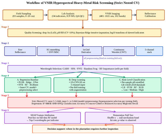
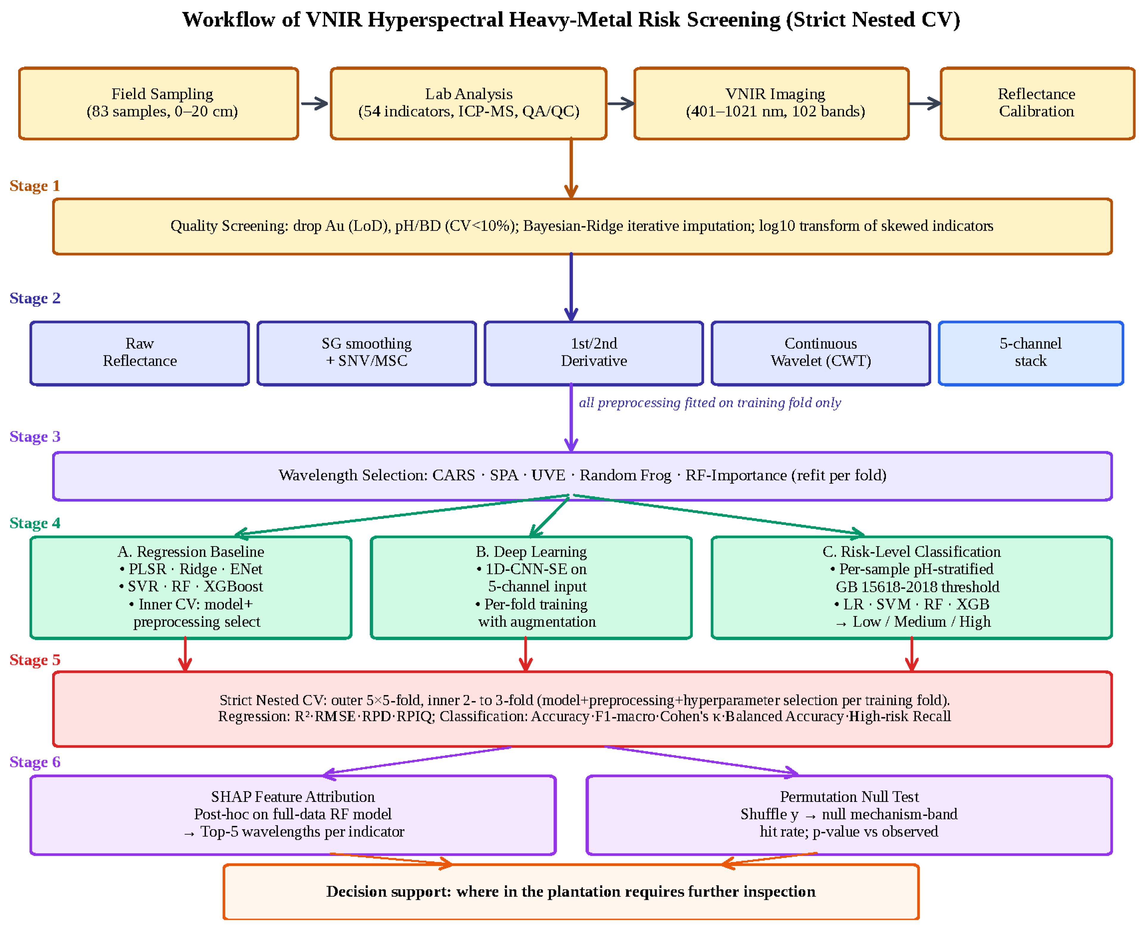
Risk-level classification (Branch C) re-cast ten heavy metals (Pb, As, Cd, Cr, Cu, Zn, Ni, Sb, Mo, Sn) as classification targets. For Pb, As, Cd, Cr, Cu, Zn, and Ni, per-sample pH-stratified thresholds from GB 15618-2018 were applied (pH < 5.5: Pb 70, As 40, Cd 0.3, Cr 150, Cu 50, Zn 200, Ni 60 mg/kg; 5.5 ≤ pH < 6.5: Pb 90, As 40, Cd 0.3, Cr 150, Cu 50, Zn 200, Ni 70 mg/kg). Mercury was excluded from regulatory screening classification because total Hg ranged from 0.036 to 0.938 mg/kg, below the lowest applicable risk screening value of 1.3 mg/kg; the high-risk class was therefore absent and high-risk recall was undefined. Three classes were defined as low (<threshold/3), medium (threshold/3 to threshold), and high (≥threshold), with automatic fallback to binary classification (high-risk vs. not) when the smallest class contained fewer than 5 samples. For Sb, Mo, and Sn, which lack national agricultural soil thresholds, 33% and 67% sample quantile boundaries defined three relative concentration tiers; these are reported as relative tiers rather than regulatory risk levels. Four classifiers were evaluated within the same nested CV protocol: Logistic Regression with balanced class weights, SVC-RBF with balanced weights, Random Forest, and XGBoost. Performance was reported using accuracy, F1-macro, Cohen’s κ, balanced accuracy, and high-risk recall, The complete analytical workflow is summarized in Figure 2.

Figure 2. Methodological workflow under the strict nested cross-validation protocol. Stage 1: field sampling (n = 83), reference chemical analysis with QA/QC, and VNIR imaging at approximately 401–1022 nm. Stage 2: quality screening, Bayesian ridge iterative imputation (refit per outer training fold), and log10 transformation of skewed indicators. Stage 3: five spectral preprocessing pipelines and a 5-channel multi-input stack for deep learning, all fitted per training fold. Stage 4: five wavelength selection algorithms refit per training fold. Stage 5: three modeling branches under outer 5 × 5-fold CV with inner 2- to 3-fold model and hyperparameter selection. Stage 6: exploratory post hoc SHAP attribution on a full-data Random Forest with a target shuffling null comparison; this stage is separate from the nested predictive evaluation.

2.8. Interpretation Framework

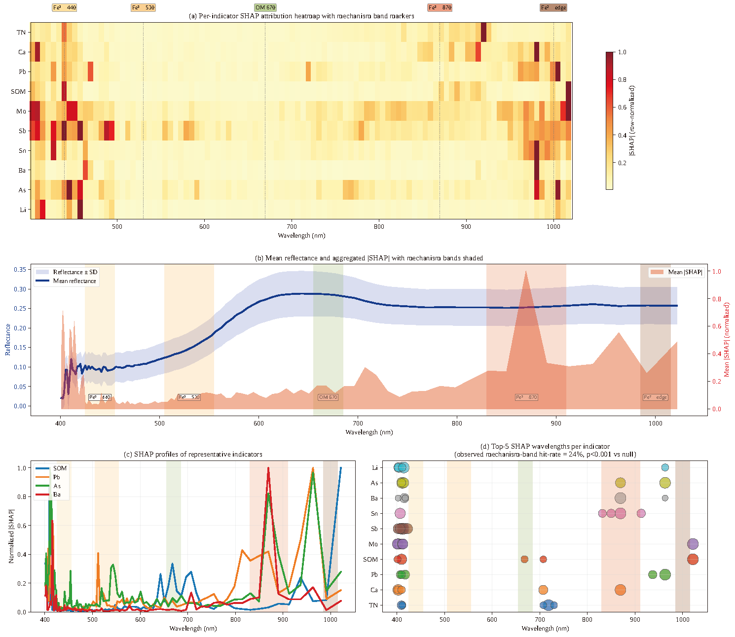
SHAP feature attribution values [41,42] were computed via TreeSHAP on a Random Forest trained once on the complete dataset after the nested predictive evaluation. This full-data analysis was not nested and had no independent held-out attribution set; it is therefore explicitly exploratory and is used only to identify plausible spectral proxy regions, not to estimate predictive performance, demonstrate generalizability, or infer causal mechanisms [52]; SHAP describes how this fitted model uses spectral features, not how underlying soil chemical processes generate the target. Per-indicator wavelength importance was computed as the mean absolute SHAP value across all 83 samples. Five mechanism bands established in the soil spectroscopy literature were used as reference targets: Fe^{3+ 6}A → ⁴T₂ (440 ± 15 nm), Fe^{3+ 6}A → ⁴T₁ visible (530 ± 25 nm), organic matter/chlorophyll (670 ± 15 nm), Fe^{3+ 6}A → ⁴T₁ NIR (870 ± 40 nm), and Fe²⁺ edge (1000 ± 15 nm) [8,17]. To assess whether the observed mechanism band hit rate was more frequent than under target-shuffled reference conditions, we constructed an empirical null distribution by randomly permuting the target values of all 10 focus indicators and recomputing the top five SHAP wavelength assignments; this procedure was repeated 50 times, yielding an empirical null distribution against which the observed hit rate was tested. With 50 permutations the smallest attainable permutation p-value is 1/(50 + 1) = 0.020; reported p-values are therefore bounded below by this value and should be read as evidence that the observed hit rate falls outside the entire null range, not as a precise conventional significance level. This comparison is conditional on the full-data Random Forest and does not convert the attribution analysis into an independent validation test.

2.9. Evaluation Metrics

Regression performance was reported as the coefficient of determination (R²), root mean square error (RMSE), ratio of performance to deviation (RPD = SD/RMSE), and ratio of performance to interquartile range (RPIQ), all computed on the log-transformed scale at which the models were fitted. A single dataset-level SD was used in the RPD denominator to provide a common descriptive scale across the 25 small outer test folds; this SD was used only in reporting and did not enter model fitting, preprocessing, or hyperparameter selection. Because RPD is referenced to that fixed dataset-level SD whereas R² is referenced to the variance of each outer test fold, the metrics are not algebraically interchangeable across folds and are interpreted jointly [53,54]. The RPD = 1.4 value is used here only as an empirical interpretive benchmark for limited or rough prediction, not as a universal acceptable prediction threshold. RPD categories depend on dataset variance and range, response transformation, preprocessing, and application context; accordingly, conclusions are based jointly on RPD, fold-wise R², RPIQ, uncertainty, and the intended screening task. RPD ≥ 2.0 is shown only as a historical reference for stronger prediction. Classification performance used accuracy, F1-macro, Cohen’s κ, balanced accuracy, and high-risk recall. For Cr and Zn, high-risk recall is descriptive for the few observed high-risk samples and is not treated as a population screening sensitivity estimate.

3. Results

3.1. Soil Indicator Distributions

The 51 retained modeling indicators, together with pH and BD as contextual properties, displayed wide chemical and statistical variability across the 83 plantation samples (Table 1). Soil pH ranged from 4.39 to 6.18 (mean 5.12, CV 6.8%), confirming acidic conditions, and BD ranged from 1.35 to 1.58 g/cm³ (mean 1.46, CV 4.6%); 71 samples had pH < 5.5 and 12 samples had 5.5 ≤ pH < 6.5, motivating the per-sample pH-stratified threshold application in the classification analysis (Section 2.7). Among basic fertility indicators, SOM averaged 29.8 g/kg (CV 42.6%), TN averaged 2374 mg/kg (CV 58.3%), and AP averaged 70.5 mg/kg (CV 102.5%), all log-transformed prior to modeling. Among heavy metals, Pb averaged 30.3 mg/kg, Cd 0.19 mg/kg, As 42.3 mg/kg, and Hg 0.150 mg/kg. Benchmarked directly against the per-sample pH-stratified GB 15618-2018 risk screening values, 19 of the 83 plots (22.9%) exceeded the As value of 40 mg/kg, 13 (15.7%) exceeded the Cd value of 0.3 mg/kg, nine (10.8%) exceeded the Cu value of 50 mg/kg, three (3.6%) exceeded the pH-stratified Pb value, two (2.4%) exceeded the Cr value of 150 mg/kg and one (1.2%) exceeded the Zn value of 200 mg/kg, whereas no sample exceeded the Ni value and the maximum Hg concentration (0.938 mg/kg) remained below the lowest applicable Hg risk screening value of 1.3 mg/kg. The As exceedance rate is considerably higher than the regional background reported for Zhejiang agricultural soils [6] and, because C. oleifera is cultivated here as a food oil crop within a designated geographic indication zone, constitutes a plantation management finding of independent interest. Several elements additionally display extreme upper tails (As 583 mg/kg, Cr 857 mg/kg, Cu 488 mg/kg, Zn 724 mg/kg, V 3150 mg/kg) consistent with localized geogenic or anthropogenic enrichment; these samples satisfied the same batch QA/QC criteria as the remainder of the dataset (Section 2.2) and were retained without modification, but their leverage on both the regression and the classification results is noted where relevant. Forty of the 51 retained indicators showed skewness > 1 and required log-transformation, reflecting the typical right-skew distribution of trace constituents in plantation-scale soil chemistry. Several trace elements (notably Sn, with a sample minimum of 3.00 mg/kg coinciding with the ICP-MS detection limit) display left-censored distributions in which a moderate fraction of values lie at or near the analytical floor; this constrains the achievable signal-to-noise for spectral inversion and likely contributes to the near-chance Sn risk-tier classification reported in Section 3.6.

Table 1. Descriptive statistics of the 51 retained modeling indicators and two contextual soil properties (n = 83).

Indicator	Unit	Min	Max	Mean	Median	SD	CV (%)	Skew.	Kurt.
pH	unitless	4.39	6.18	5.12	5.07	0.348	6.79	0.534	0.126
BD	g/cm3	1.35	1.58	1.46	1.46	0.0681	4.65	−0.047	−1.10
SOM	g/kg	8.19	92.5	29.8	29.3	12.7	42.6	1.46	5.37
TP	mg/kg	55.7	2.61 × 103	554	474	425	76.7	2.55	8.39
TN	mg/kg	503	9.35 × 103	2.37 × 103	2.22 × 103	1.38 × 103	58.3	1.99	6.65
AP	mg/kg	9.30	369	70.5	44.0	72.3	102.5	2.07	4.03
AK	mg/kg	9.10	62.4	23.0	22.3	8.60	37.3	1.87	5.91
HN	mg/kg	60.3	173	98.3	90.1	30.4	30.9	0.77	−0.41
Li	mg/kg	1.74	146	35.8	28.7	25.4	71.1	1.52	3.08
Na	mg/kg	611	3.48 × 103	1.47 × 103	1.34 × 103	515	35.1	1.00	1.51
Mg	mg/kg	1.40 × 103	1.52 × 104	3.29 × 103	3.07 × 103	1.71 × 103	51.9	4.24	26.58
Al	mg/kg	3.50 × 104	9.05 × 104	5.88 × 104	5.73 × 104	1.03 × 104	17.6	0.37	0.26
K	mg/kg	8.94 × 103	5.56 × 103	1.93 × 104	1.82 × 104	7.99 × 103	41.4	2.24	7.36
Ca	mg/kg	161	9.29 × 103	1.13 × 103	627	1.58 × 103	139.9	3.69	14.83
Ti	mg/kg	1.76 × 103	6.53 × 103	4.01 × 103	3.77 × 103	947	23.6	0.45	0.16
V	mg/kg	25.2	3.15 × 103	153	92.1	388	253.1	6.71	45.23
Cr	mg/kg	15.7	857	68.5	57.4	93.8	137.0	7.40	57.89
Mn	mg/kg	28.3	3.22 × 103	451	339	438	97.0	3.36	17.25
Fe	mg/kg	1.00 × 104	4.48 × 104	2.51 × 104	2.45 × 104	6.80 × 103	27.1	0.11	0.43
Co	mg/kg	1.77	30.6	10.9	10.1	5.74	52.4	0.62	0.24
Ni	mg/kg	5.40	57.3	26.8	27.5	10.8	40.4	0.30	0.35
Cu	mg/kg	5.29	488	35.5	28.9	52.0	146.3	7.92	65.89
Zn	mg/kg	21.1	724	84.6	70.5	76.9	90.9	6.95	54.65
As	mg/kg	4.14	583	42.3	23.7	72.6	171.6	5.40	35.03
Se	mg/kg	0.610	31.6	4.18	3.43	3.83	91.5	4.56	29.13
Rb	mg/kg	2.25 × 103	5.11 × 104	9.30 × 103	7.55 × 103	7.26 × 103	78.0	3.47	15.29
Sr	mg/kg	6.46	165	38.8	25.3	35.3	91.0	1.96	3.01
Y	mg/kg	1.89	73.2	14.5	11.8	10.8	74.4	2.89	11.49
Zr	mg/kg	114	288	177	170	39.4	22.3	0.60	−0.17
Mo	mg/kg	0.420	80.8	4.86	1.21	11.4	235.0	5.21	28.97
Rh	mg/kg	7.29	203	83.0	73.5	43.2	52.1	0.69	0.13
Ag	mg/kg	0.430	11.5	1.34	1.05	1.32	98.6	5.95	40.39
Cd	mg/kg	0.0400	0.910	0.189	0.150	0.146	77.2	2.72	10.20
Sn	mg/kg	3.00	67.9	7.34	4.63	9.32	126.9	4.48	22.18
Sb	mg/kg	0.800	32.2	4.38	2.70	5.08	115.9	3.13	11.70
Cs	mg/kg	4.96	38.5	11.3	10.9	5.04	44.6	2.59	10.80
Ba	mg/kg	107	8.82 × 103	897	391	1.46 × 103	162.4	3.51	13.03
La	mg/kg	2.81	118	29.9	24.9	18.7	62.4	1.54	4.56
Ce	mg/kg	6.72	156	71.4	66.0	34.2	47.8	0.19	−0.47
Pr	mg/kg	0.990	24.4	7.39	6.96	3.89	52.6	1.21	3.23
Nd	mg/kg	4.51	94.2	28.5	26.6	14.6	51.4	1.30	3.72
Sm	mg/kg	1.20	15.6	5.62	5.20	2.70	48.0	1.12	2.30
Eu	mg/kg	0.230	3.19	1.08	1.00	0.500	46.3	1.19	2.83
Gd	mg/kg	1.09	15.4	4.71	4.12	2.40	50.9	1.55	4.20
Tb	mg/kg	13.2	85.3	53.8	55.3	15.4	28.6	−0.21	−0.52
Dy	mg/kg	0.910	11.9	3.76	3.38	1.98	52.5	1.87	5.09
Ho	mg/kg	0.180	2.58	0.760	0.670	0.415	54.7	2.16	6.79
Er	mg/kg	0.0200	0.320	0.0966	0.0900	0.0524	54.2	2.05	6.16
Tm	mg/kg	0.110	1.72	0.374	0.330	0.218	58.3	3.37	16.54
Yb	mg/kg	0.820	12.9	2.60	2.32	1.59	60.9	3.74	20.00
Hg	mg/kg	0.0360	0.938	0.150	0.117	0.144	95.7	3.62	13.83
TI	mg/kg	0.490	5.00	1.43	1.07	0.842	59.0	1.83	3.56
Pb	mg/kg	13.5	103	30.3	26.1	14.5	47.8	2.82	9.01

3.2. Spectral Characteristics and Intrinsic Dimensionality

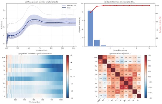
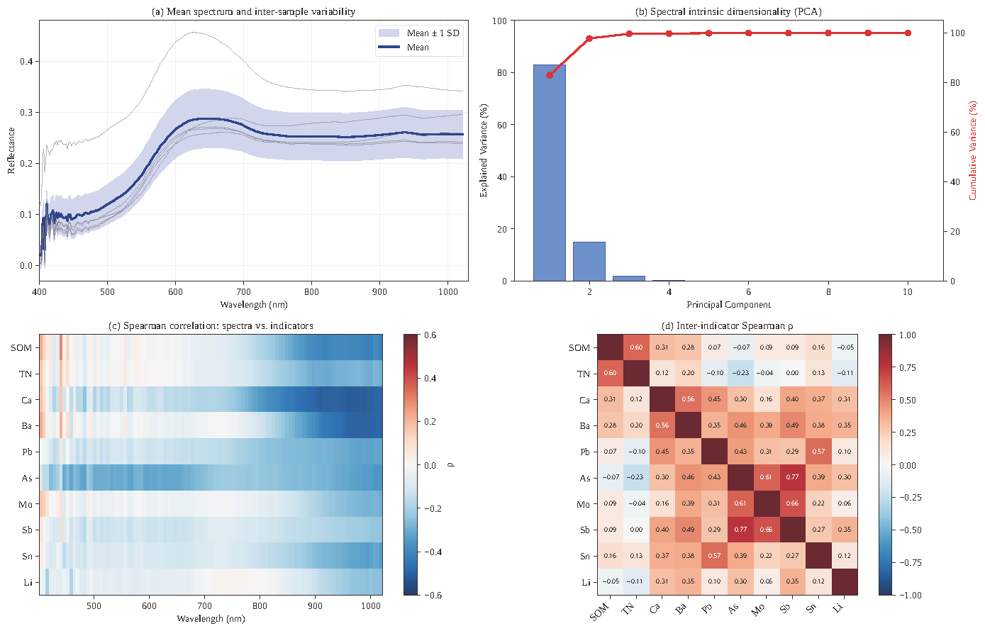
Mean reflectance and inter-sample variability (Figure 3a) showed a typical red soil spectral signature: low reflectance below 500 nm (≈10%), a steady rise across the visible-to-NIR transition centered near 600 nm, and a broad NIR plateau between 800 and 1000 nm (mean ≈ 26%). Principal component analysis revealed that the 102-band reflectance matrix concentrated 95% of its variance in the first two components (PC1: 82.9%; PC2: 14.9%); the first three components explained 99% (Figure 3b). This effectively two- to three-dimensional intrinsic structure suggests a limited spectral information space that may partly explain the modest predictive performance documented below.

Figure 3. Spectral characteristics and correlation diagnostic. (a) Mean reflectance spectrum with ±1 SD shaded band; (b) explained-variance ratios of the first 10 principal components (blue bars) and cumulative explained variance (red line, right axis), showing an intrinsic dimensionality of two to three; (c) Spearman correlations between each of 102 spectral bands and each of 10 focus indicators; (d) inter-indicator Spearman correlation matrix showing geochemical clustering.

Spectrum indicator correlations were at most moderate (Figure 3c). The maximum Spearman correlation between any band and any focus indicator was |ρ| = 0.515 (Ca at 814 nm), and only Ca and Ba showed at least 25 bands with |ρ| > 0.3. For Mo and Sb, no single band reached |ρ| = 0.30; predictions for these elements thus rely entirely on indirect co-variation. By contrast, indicator co-variation revealed clearly interpretable geochemical clusters (Figure 3d): Mo–Sb–As (ρ = 0.61–0.77), Pb–Sn (ρ = 0.57), Ba–Ca (ρ = 0.56), and SOM–TN (ρ = 0.60).

3.3. Strict Nested CV Yields Low Observed Regression Performance

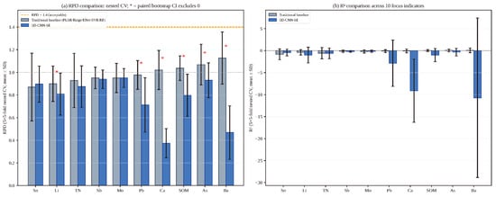
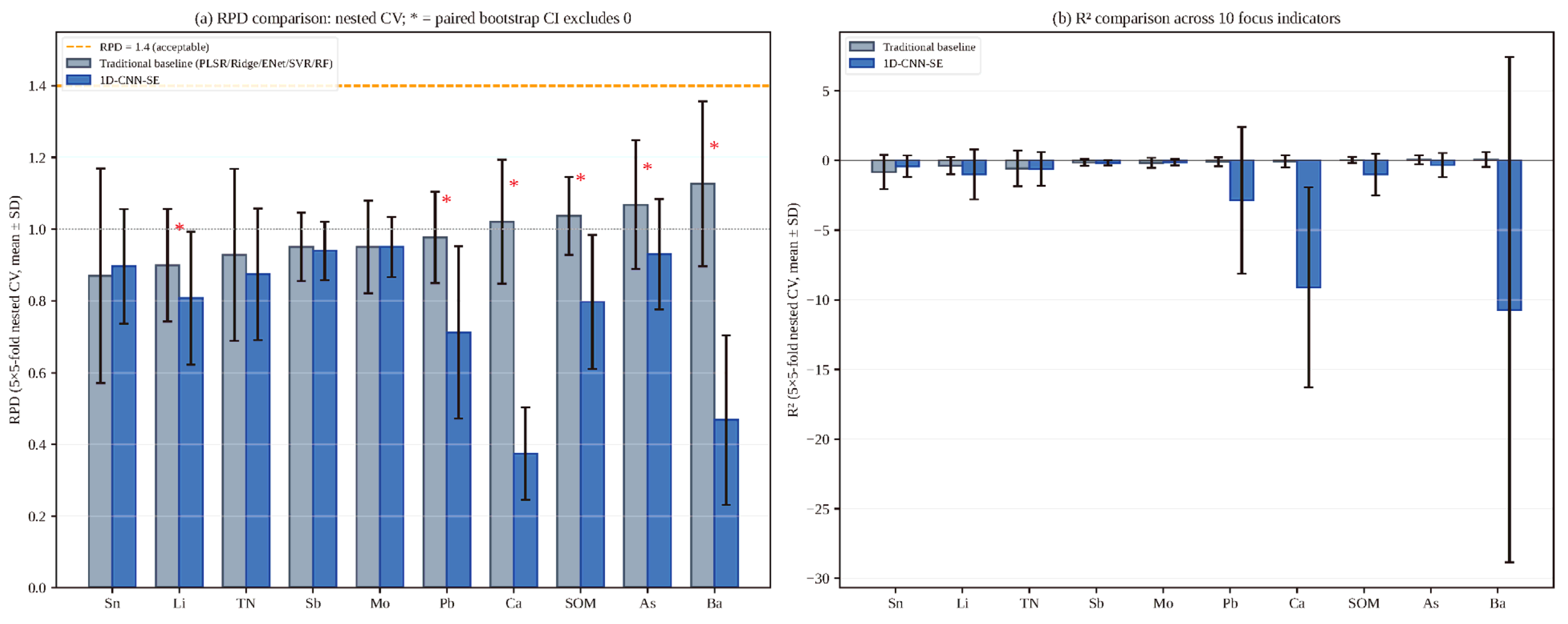
Under the strict nested cross-validation protocol (Table 2; Figure 4), no focus indicator reached the empirical RPD = 1.4 interpretive benchmark. The highest observed mean RPD was Ba = 1.127 ± 0.231 (PLSR with n_components = 3 on SG + FD-preprocessed spectra), followed by As = 1.068 ± 0.180 (Ridge on raw), SOM = 1.037 ± 0.108 (Random Forest on SG + FD), and Ca = 1.021 ± 0.173 (ElasticNet on raw). Mean fold-wise R² values were modest and frequently negative (range −0.578 to 0.070), indicating that the held-out fold mean prediction baseline often outperformed the fitted models. The RPD benchmark is empirical and dataset-dependent; the inference of weak quantitative utility rests jointly on the RPD pattern, mostly nonpositive fold-wise R², and failure of the classification reformulation. Compared with the earlier non-nested exploratory estimates, strict nesting lowered RPD by approximately 0.10–0.15 and eliminated apparent CNN gains, a pattern consistent with inflation from non-nested preprocessing and model selection. Because the ten targets were selected using the same dataset before cross-validation, these absolute estimates remain conditional and may be optimistic; they are not presented as a universal attainable limit. Inner-CV selection most frequently chose simple linear models over tree-based or kernel methods.

Table 2. Strict nested cross-validation results for 10 focus indicators (5 repeats × 5-fold = 25 outer test sets).

Indicator	R2 Baseline	R2 1D-CNN-SE	RPD Baseline	RPD 1D-CNN-SE	ΔRPD (95% CI)	Significant
Ba	0.070 ± 0.535	−10.725 ± 18.134	1.127 ± 0.231	0.468 ± 0.236	−0.659 (−0.77, −0.55)	Yes
SOM	0.038 ± 0.214	−1.006 ± 1.493	1.037 ± 0.109	0.797 ± 0.187	−0.240 (−0.30, −0.18)	Yes
Ca	−0.062 ± 0.433	−9.098 ± 7.178	1.021 ± 0.173	0.374 ± 0.129	−0.647 (−0.73, −0.55)	Yes
As	0.047 ± 0.316	−0.336 ± 0.868	1.068 ± 0.180	0.930 ± 0.154	−0.139 (−0.24, −0.05)	Yes
Pb	−0.107 ± 0.324	−2.859 ± 5.247	0.977 ± 0.127	0.712 ± 0.240	−0.265 (−0.36, −0.18)	Yes
TN	−0.578 ± 1.289	−0.613 ± 1.222	0.929 ± 0.240	0.874 ± 0.184	−0.054 (−0.16, 0.06)	No
Mo	−0.177 ± 0.369	−0.136 ± 0.226	0.951 ± 0.130	0.950 ± 0.084	−0.000 (−0.04, 0.04)	No
Sb	−0.143 ± 0.253	−0.158 ± 0.192	0.951 ± 0.095	0.939 ± 0.081	−0.011 (−0.05, 0.03)	No
Li	−0.382 ± 0.610	−1.005 ± 1.781	0.899 ± 0.157	0.808 ± 0.186	−0.092 (−0.16, −0.02)	Yes
Sn	−0.828 ± 1.243	−0.424 ± 0.767	0.870 ± 0.299	0.896 ± 0.160	0.026 (−0.07, 0.12)	No

ΔRPD 1. D-CNN-SE − Baseline; negative values indicate the deep model is worse. Significance assessed by 1000-resample paired bootstrap of fold-level RPD differences (95% CI excludes zero).

Figure 4. Strict nested CV regression performance. (a) RPD comparison between the traditional baseline (gray; model and preprocessing selected within each outer training fold) and the 1D-CNN-SE model (blue), with error bars showing the standard deviation across 25 outer test folds and red asterisks marking indicators where the paired bootstrap 95% confidence interval excludes zero. (b) Fold-wise R² comparison. The dashed RPD = 1.4 line is an empirical interpretive benchmark rather than a universal acceptability threshold.

3.4. 1D-CNN-SE Significantly Underperforms the Linear Baseline

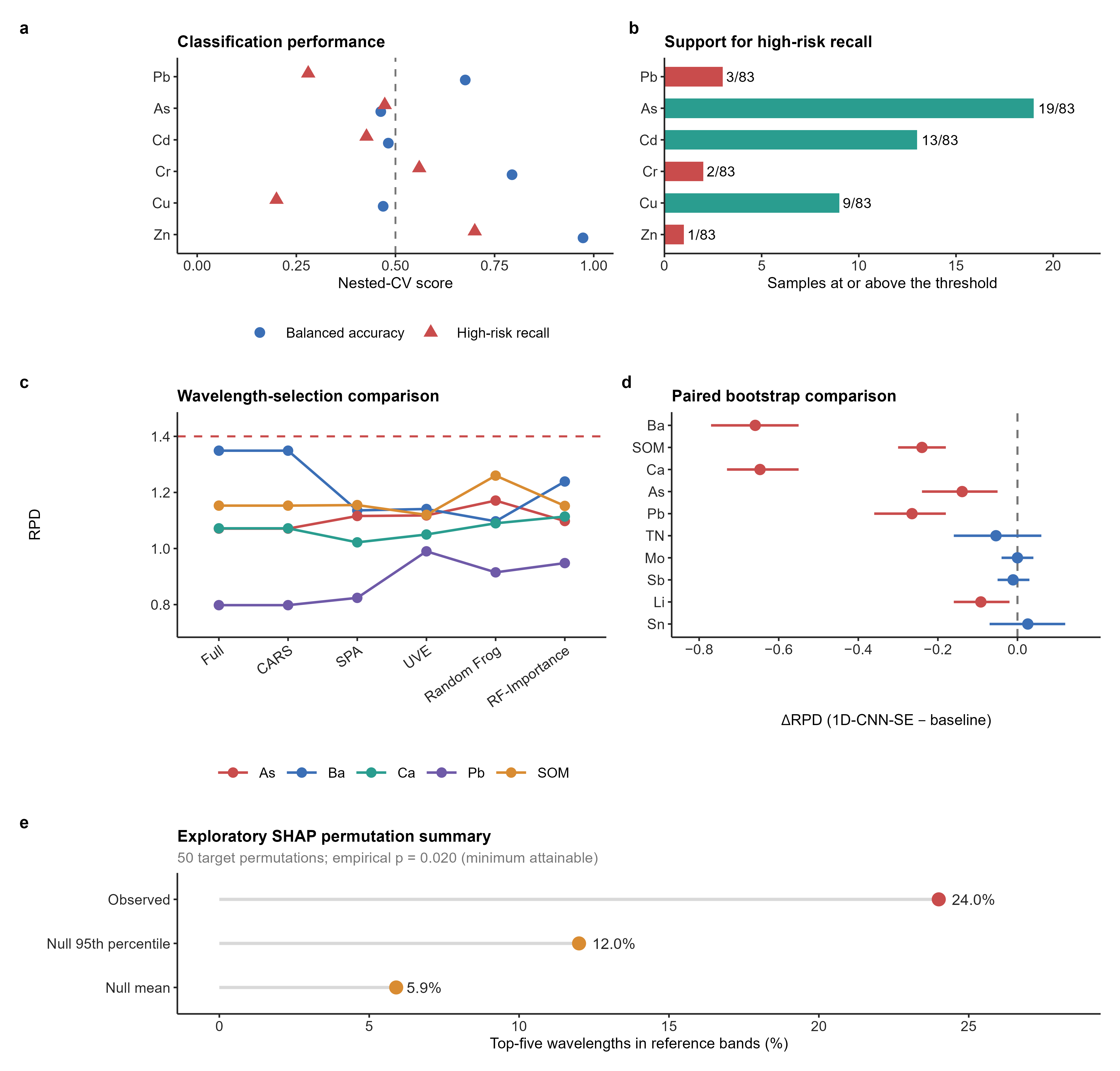
Under the strict nested CV protocol, 1D-CNN-SE on the multi-channel input performed significantly worse than the inner-CV-selected traditional baseline for 6 of 10 focus indicators (Table 2; Figure 4). The paired bootstrap 95% confidence interval excluded zero in the negative direction for Ba (ΔRPD = −0.659, CI [−0.774, −0.551]), Ca (−0.647, [−0.729, −0.552]), Pb (−0.265, [−0.363, −0.178]), SOM (−0.240, [−0.305, −0.184]), As (−0.139, [−0.240, −0.052]), and Li (−0.092, [−0.163, −0.020]). For the remaining four indicators (TN, Mo, Sb, Sn), the confidence intervals straddled zero, indicating no significant difference. No indicator showed a significant CNN-SE improvement. This is a striking departure from our earlier exploratory benchmark, which had reported small CNN-SE gains for eight of eleven indicators (mean ΔRPD = +0.060). Under strict nesting, those gains disappear or reverse, which is consistent with inflation from preprocessing and model selection bias in the original protocol. The collapse is most severe for Ca and Ba, where R² fell from positive values in the single-split benchmark to large negative values (Ca R² = −9.10, Ba R² = −10.7) under strict nesting; both indicators have the strongest spectrum signal among our targets, making them most susceptible to overfitting in a small-sample neural network with no inner regularization tuning.

3.5. Wavelength Selection Does Not Lift Observed Performance

Five wavelength-selection methods were applied to the five strongest indicators (Ba, As, Ca, SOM, Pb; Table 3, Figure 5c). Random Frog produced the most consistent gain—most notably for SOM, where R² rose from 0.244 (full spectrum) to 0.370 with 15 selected bands and RPD increased from 1.153 to 1.260. UVE substantially recovered Pb’s negative R² (from −0.590 to −0.026), suggesting that the majority of the 102 bands act as noise for Pb. CARS retained essentially the full spectrum after convergence and offered no compression in our short-wavelength setting, consistent with reports of CARS sensitivity to the relative weight of informative versus uninformative bands when the input range is dominated by structural rather than vibrational features [39]. SPA and RF-Importance gave moderate but variable gains. Importantly, no method reached the empirical RPD = 1.4 benchmark, indicating that wavelength selection reduced noise for some targets but did not materially change the overall interpretation.

Table 3. Wavelength selection methods comparison (5 seeds × 5-fold CV, PLSR).

Indicator	Method	N Bands	R2	RMSE	RPD
Ba	Full	102	0.442	0.271	1.349
Ba	CARS	102	0.442	0.271	1.349
Ba	SPA	15	0.222	0.320	1.136
Ba	UVE	16	0.231	0.319	1.141
Ba	Random Frog	15	0.161	0.332	1.097
Ba	RF Importance	15	0.347	0.294	1.239
As	Full	102	0.127	0.352	1.071
As	CARS	102	0.127	0.352	1.071
As	SPA	15	0.192	0.339	1.116
As	UVE	16	0.194	0.338	1.118
As	Random Frog	15	0.270	0.322	1.171
As	RF Importance	15	0.169	0.344	1.098
Ca	Full	102	0.128	0.325	1.072
Ca	CARS	102	0.128	0.325	1.072
Ca	SPA	15	0.043	0.340	1.022
Ca	UVE	16	0.091	0.331	1.050
Ca	Random Frog	15	0.158	0.319	1.090
Ca	RF Importance	15	0.191	0.313	1.114
SOM	Full	102	0.244	0.138	1.153
SOM	CARS	102	0.244	0.138	1.153
SOM	SPA	15	0.248	0.138	1.155
SOM	UVE	16	0.198	0.142	1.120
SOM	Random Frog	15	0.370	0.126	1.260
SOM	RF Importance	15	0.243	0.138	1.152
Pb	Full	102	−0.590	0.160	0.798
Pb	CARS	102	−0.590	0.160	0.798
Pb	SPA	15	−0.494	0.155	0.824
Pb	UVE	16	−0.026	0.129	0.990
Pb	Random Frog	15	−0.199	0.139	0.915
Pb	RF Importance	15	−0.116	0.135	0.948

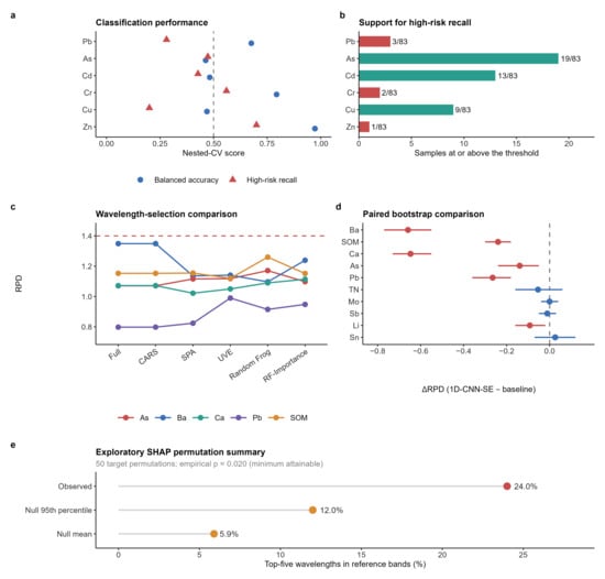
Figure 5. Clssification support, model comparisons, and exploratory SHAP summary. (a) Balanced accuracy (blue circles) and high-risk recall (red triangles) for metals with regulatory thresholds; the vertical dashed line marks 0.5. (b) Numbers of samples at or above the applicable thresholds; red bars indicate metals represented by fewer than five high-risk samples, whereas teal bars indicate metals represented by five or more high-risk samples. (c) RPD for full spectra and five wavelength-selection methods; the horizontal dashed line marks the empirical RPD = 1.4 interpretive benchmark. (d) Paired-bootstrap ΔRPD (1D-CNN-SE − baseline); the vertical dashed line marks ΔRPD = 0, red intervals exclude zero, and blue intervals include zero. (e) Exploratory full-data SHAP mechanism-band hit rate (observed 24.0%) compared with the target-permutation null mean (5.9%) and 95th percentile (12.0%). With 50 permutations, empirical p = 0.020 is the minimum attainable value. This post hoc analysis does not provide independent evidence of predictive generalizability.

3.6. Risk-Level Classification Does Not Recover Operational Screening Capability

Reformulating ten heavy metals as a risk-level classification problem under per-sample pH-stratified GB 15618-2018 thresholds did not recover operational utility, and the apparent heterogeneity across metals is largely a function of how many exceeding samples each metal contributes (Table 4; Figure 5a,b). Two metals returned nominally high scores: Cr (binary classification, balanced accuracy 0.794, high-risk recall 0.560, accuracy 0.969) and Zn (binary classification, balanced accuracy 0.973, high-risk recall 0.700, accuracy 0.973). These figures must, however, be read against their support: the Cr and Zn high-risk classes contain two and one samples, respectively, out of 83, so the recall values summarize repeated recovery of those individual observations across the 25 outer folds. They do not provide stable estimates of population screening sensitivity and are reported only descriptively, not as demonstrated screening capability. Three metals with more substantial high-risk support occupied a middle tier and are correspondingly more informative, but performed poorly: As (three-class, 19 exceeding samples, balanced accuracy 0.463, κ 0.162, high-risk recall 0.473), Cd (three-class, 13 exceeding samples, balanced accuracy 0.482, κ 0.170, high-risk recall 0.427), and Cu (three-class, nine exceeding samples, balanced accuracy 0.469, κ 0.201, high-risk recall 0.200). For these three metals, where the class structure is stable enough to support inference, balanced accuracy remains close to the 0.33 chance level of a three-class problem and Cohen’s κ does not exceed 0.21, well below the κ = 0.4 moderate agreement criterion adopted in Section 2.9. The remaining metals were not evaluable: Pb showed high binary accuracy (0.938) but high-risk recall of only 0.280 with three exceeding samples; Mo, Sb, and Sn (relative-tier classification using 33%/67% quantiles) reached only κ = −0.019 to 0.106, at or below random performance despite balanced class sizes; and Ni had no samples exceeding the pH-stratified value, collapsing to a single-class problem. The Mo, Sb, and Sn results are the most diagnostic of the three groups, because their quantile-defined tiers are balanced by construction and therefore free of the imbalance artefacts that complicate the regulatory threshold metals; that these balanced problems remain at chance indicates an absence of recoverable spectral signal rather than a class distribution artefact.

Table 4. Risk-level classification performance under strict nested CV (5 repeats × 5-fold stratified).

Metal	Classes	Scheme	Accuracy	Macro-F1	Cohen’s κ	Balanced Acc	HR-Recall	HR n/Total
Pb	2	pH-stratified GB + GB/3	0.938	0.623	NA	0.676	0.280	3/83
As	3	pH-stratified GB + GB/3	0.470	0.450	0.162	0.463	0.473	19/83
Cd	3	pH-stratified GB + GB/3	0.501	0.448	0.170	0.482	0.427	13/83
Cr	2	pH-stratified GB + GB/3	0.969	0.772	NA	0.794	0.560	2/83
Cu	3	pH-stratified GB + GB/3	0.682	0.438	0.201	0.469	0.200	9/83
Zn	2	pH-stratified GB + GB/3	0.973	0.843	NA	0.973	0.700	1/83
Ni	1	pH-stratified GB + GB/3	NA	NA	NA	NA	NA	0/83
Sb	3	33%/67% quantile	0.404	0.385	0.106	0.400	0.459	29/83
Mo	3	33%/67% quantile	0.322	0.308	−0.019	0.318	0.395	28/83
Sn	3	33%/67% quantile	0.396	0.375	0.094	0.396	0.483	28/83

NA, not applicable: Cohen’s κ is undefined when a fold-level classifierpredicted a single class; for Ni, the threshold produced fewer than two classes.

The pooled predictions underlying Table 4 indicate that the models sometimes recovered the very small Cr and Zn high-risk subsets, but with only two and one unique exceeding samples this behavior cannot be established statistically or generalized to a target population. Figure 5b therefore foregrounds the number of samples supporting each recall value. The Pb result likewise illustrates why accuracy alone is inadequate: a model that predicts “safe” for nearly all plots can score highly while remaining operationally ineffective at identifying samples that require confirmatory chemical analysis.

Per-sample pH-stratified GB 15618-2018 risk screening values were applied to Pb, As, Cd, Cr, Cu, Zn, and Ni; 33%/67% sample quantiles were applied to Sb, Mo, and Sn as relative tiers, not regulatory values. Hg is not listed because its observed range (0.036–0.938 mg/kg) contained no sample at or above the lowest applicable GB risk screening value of 1.3 mg/kg, leaving no high-risk class. The best classifier per metal was selected by F1-macro within nested CV. HR n/total is the number of samples at or above the applicable threshold. Cohen’s κ is reported as NA for binary problems when a fold level classifier predicted a single class; balanced accuracy and high-risk recall are reported instead. NA for Ni indicates that the regulatory threshold produced fewer than two classes. Cr and Zn recall values are descriptive of two and one high-risk samples, respectively, and cannot estimate population screening sensitivity.

3.7. Exploratory SHAP Attribution Identifies Plausible Proxy Regions

Exploratory TreeSHAP attribution from a Random Forest trained on the full dataset (Figure 6) showed that 12 of 50 top-five wavelengths across the 10 focus indicators (24%) fell within the predefined Fe-oxide or organic matter reference bands. The empirical target permutation comparison had a null mean of 5.9% and a 95th percentile of 12.0%, below the observed 24% (empirical p = 0.020, the minimum attainable with 50 permutations; Figure 5e). The cross-indicator mean |SHAP| spectrum showed local importance near 870 nm, near the upper spectral edge, and in the 400–460 nm region. Per-indicator patterns placed Sn, Ba, and Pb near the 869 nm Fe-related region and assigned As to both visible and NIR regions (Table 5). These are plausible model-based spectral proxy regions, not direct evidence of Fe-oxide or organic matter control. Because the Random Forest was fitted to all 83 samples after the nested predictive evaluation and no held-out attribution set was used, the SHAP results provide neither causal evidence nor independent evidence of predictive generalizability. The permutation comparison only indicates that attribution alignment was more frequent than under target shuffling for this fitted model.

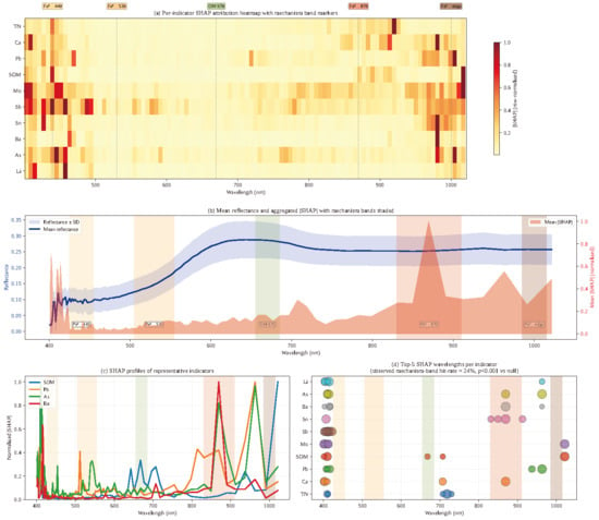
Figure 6. Exploratory SHAP feature attribution from a Random Forest trained on all 83 samples. (a) Per-indicator SHAP heatmap with predefined reference band markers; (b) mean reflectance ± SD overlaid with aggregated |SHAP| and shaded reference bands; (c) SHAP profiles for representative indicators; (d) top five SHAP wavelengths per indicator. Colors: in (a), the yellow-to-dark-red scale gives the row-normalized mean |SHAP| (color bar); in (b), the blue line and envelope are mean reflectance ± 1 SD (left axis) and the orange curve is aggregated |SHAP| (right axis); in (c,d), color distinguishes indicators; shaded bands and dashed lines mark the five reference wavelength windows. The observed 24% reference band hit rate exceeded the 5.9% target permutation null mean (50 permutations; empirical p = 0.020, the minimum attainable). This post hoc full-data attribution identifies plausible proxy regions and is not an independent validation of predictive generalizability or a causal mechanism test.

Table 5. Top-3 SHAP-attributed wavelengths per indicator and their mechanism band assignment.

Indicator	Top 1	Mechanism	Top 2	Mechanism	Top 3	Mechanism
TN	718 nm	—	410 nm	—	707 nm	—
Ca	869 nm	Fe3+ 870 nm	403 nm	—	707 nm	—
Pb	963 nm	—	417 nm	Fe3+ 440 nm	937 nm	Fe3+ 870 nm
SOM	1022 nm	Fe2+ edge	410 nm	—	401 nm	—
Mo	1022 nm	Fe2+ edge	403 nm	—	401 nm	—
Sb	410 nm	—	414 nm	Fe3+ 440 nm	422 nm	Fe3+ 440 nm
Sn	869 nm	Fe3+ 870 nm	407 nm	—	850 nm	Fe3+ 870 nm
Ba	869 nm	Fe3+ 870 nm	416 nm	Fe3+ 440 nm	417 nm	Fe3+ 440 nm
As	411 nm	Fe3+ 440 nm	963 nm	—	869 nm	Fe3+ 870 nm
Li	414 nm	Fe3+ 440 nm	404 nm	—	403 nm	—

Mechanism 440. nm = ±15; Fe³⁺ 530 = ±25; OM 670 = ±15; Fe³⁺ 870 = ±40; Fe²⁺ edge 1000 = ±15. Em-dash indicates no mechanism band within tolerance. The original unrounded wavelength vector was not available in the retained study records; 1022 nm is retained as the stored rounded upper-edge band label, and spectral coverage is therefore reported approximately (Section 2.3).

Table 5. Top-3 SHAP-attributed wavelengths per indicator and their mechanism band assignment.

Indicator	Top 1	Mechanism	Top 2	Mechanism	Top 3	Mechanism
TN	718 nm	—	410 nm	—	707 nm	—
Ca	869 nm	Fe3+ 870 nm	403 nm	—	707 nm	—
Pb	963 nm	—	417 nm	Fe3+ 440 nm	937 nm	Fe3+ 870 nm
SOM	1022 nm	Fe2+ edge	410 nm	—	401 nm	—
Mo	1022 nm	Fe2+ edge	403 nm	—	401 nm	—
Sb	410 nm	—	414 nm	Fe3+ 440 nm	422 nm	Fe3+ 440 nm
Sn	869 nm	Fe3+ 870 nm	407 nm	—	850 nm	Fe3+ 870 nm
Ba	869 nm	Fe3+ 870 nm	416 nm	Fe3+ 440 nm	417 nm	Fe3+ 440 nm
As	411 nm	Fe3+ 440 nm	963 nm	—	869 nm	Fe3+ 870 nm
Li	414 nm	Fe3+ 440 nm	404 nm	—	403 nm	—

Mechanism 440. nm = ±15; Fe³⁺ 530 = ±25; OM 670 = ±15; Fe³⁺ 870 = ±40; Fe²⁺ edge 1000 = ±15. Em-dash indicates no mechanism band within tolerance. The original unrounded wavelength vector was not available in the retained study records; 1022 nm is retained as the stored rounded upper-edge band label, and spectral coverage is therefore reported approximately (Section 2.3).

4. Discussion

4.1. Strict Nesting Lowers Observed Performance Estimates

The most important methodological finding of this study is that strict nested cross-validation reduces the apparent regression performance by approximately 0.10–0.20 RPD points relative to single-split or non-nested protocols, lowering the highest observed mean RPD from approximately 1.35 (1D-CNN-SE in the exploratory analysis) to 1.13 (Ba; traditional baseline) under strict nesting. Crucially, the gap is large enough to change qualitative interpretation: while the exploratory benchmark suggested 1D-CNN-SE provided modest but consistent gains over traditional baselines, strict nested CV reveals that the deep model performs significantly worse for six of 10 indicators and never significantly better. This reversal does not reflect a flaw in deep learning per se; rather, it demonstrates how small-sample VNIR studies that do not nest preprocessing, imputation, scaling, and model selection within outer folds can overestimate performance and can incorrectly suggest gains from complex methods. Our finding aligns with well-established cautionary reports on nested cross-validation in the broader machine-learning and chemometrics literature: Cawley and Talbot [55] demonstrated that hyperparameter selection performed outside an outer cross-validation loop systematically inflates apparent performance even on synthetic data with no genuine signal, and Vabalas et al. [56] documented inflated performance estimates of approximately 0.10–0.20 in classification accuracy under non-nested protocols across simulated and real biomedical datasets—a magnitude closely matching the 0.10–0.20 RPD inflation we observe here. These findings reinforce the methodological conclusion that benchmark studies on small-sample soil spectra should default to strict nesting with paired statistical comparisons. The empirical RPD = 1.4 benchmark is not treated as universal; the present interpretation also rests on mostly nonpositive fold-wise R², uncertainty across folds, and failure of the risk classification reformulation.

4.2. Indirect Fe–OM Coupling Explains the Limited Prediction Upper Bound

The exploratory SHAP analysis suggests that VNIR-based prediction of low-concentration heavy metals in C. oleifera red soils relies primarily on co-variation with Fe-oxides and organic matter rather than direct spectral absorption [11,13]. Iron oxides exhibit strong electronic transition absorption near 440 nm, 530 nm, and 870 nm [17]; organic matter suppresses overall reflectance throughout the 550–770 nm range; both constituents act as scavengers for Pb, Cd, As, and other trace metals through surface complexation, ion exchange, and precipitation under the acidic red soil conditions characteristic of our study area [6,9]. The attribution of Sn, Ba, and Pb near the 870 nm Fe³⁺ NIR region, and of SOM and As to visible and NIR regions, is physically plausible and provides limited face validity to the model attributions. Importantly, we frame this as model attribution alignment rather than causal mechanism evidence: the data-driven attributions tell us how the model exploits spectral features [57], while the mechanistic interpretation requires independent corroboration from soil chemical fractionation studies. The indirect coupling mode bounds the achievable accuracy upper bound: where Fe-OM-Pb coupling is weakest (e.g., recently disturbed soils, calcareous substrates, or non-pedogenic mineral assemblages), the same models should fail. Beyond the present application, the combination of SHAP attribution with a target shuffling permutation null distribution constitutes a transferable physical plausibility test for small-sample soil spectroscopy models: hit rates that significantly exceed the null indicate that model attribution is anchored to established mechanism bands rather than to spurious sample-level correlations, providing an exploratory attribution plausibility check that does not depend on access to large external libraries. It does not test out-of-sample predictive generalizability.

The measured soil context is consistent with important constraints on both metal behavior and VNIR response: pH was uniformly acidic (4.39–6.18), while SOM varied from 8.19 to 92.5 g/kg. These measured gradients can affect sorption and broad reflectance patterns and may contribute to indirect covariance between spectra and metals. However, plot-level cation exchange capacity, texture, mineralogical composition, and iron oxide forms were not measured. Their separate contributions cannot be resolved here, and the SHAP regions should not be used to infer those unmeasured pedological properties.

4.3. Risk-Level Reformulation and the Limits of the Present Evidence

Re-formulating heavy metal prediction as risk-level classification is frequently proposed as the pragmatic response to weak regression performance, on the reasoning that a coarse three-level judgement demands less of the spectrum than a concentration estimate. The present results do not support that expectation at this sample size. Where the classification problem is balanced by construction and therefore interpretable—the relative-tier targets Mo, Sb and Sn, each with approximately 28 samples per tier—performance sits at chance (κ = −0.019 to 0.106). Where the problem is defined by regulatory thresholds and retains adequate support—As, Cd and Cu, with 19, 13 and nine exceeding samples—balanced accuracy remains near the three-class chance level and κ does not exceed 0.21. The two metals with nominally strong scores, Cr and Zn, are precisely the two with the smallest high-risk support (two and one samples), and their recall values are therefore descriptions of individual samples rather than estimates of a population-level screening rate. Reading them as evidence of screening capability would repeat, at the level of class support, the same over-interpretation that this study documents at the level of cross-validation design.

The Pb result illustrates why accuracy alone is inadequate for screening applications. Pb’s apparent accuracy of 0.938 is driven by class imbalance—only three of 83 samples fall at or above the per sample threshold—and is achieved principally by predicting “safe” for nearly every plot; the corresponding high-risk recall of 0.280 implies that most exceeding plots would be missed. In a food safety screening context a false negative rate of this magnitude is disqualifying, yet the accuracy figure alone would present the model favorably. The practical recommendation that follows is therefore not a list of metals for which VNIR screening can be deployed, but a reporting requirement: studies proposing spectral risk screening should state the number of exceeding samples underlying every recall estimate and should report balanced accuracy and high-risk recall alongside accuracy, so that imbalance-driven results cannot be mistaken for screening capability. From the present evidence, no metal in this dataset meets a defensible standard for operational deployment, and establishing whether Cr and Zn merit further investigation requires an independent dataset containing a substantially larger contaminated subset.

4.4. Limitations and Directions for Future Work

Several limitations should be acknowledged. The sample size of 83 is modest, and although strict nested cross-validation provides robust point estimates, performance estimates may shift as additional samples are added; future work should expand the sample base to 200–500 spanning multiple plantation regions. Critically, the favorable screening claims for Cr and Zn rest on only two and one high-risk samples respectively under the pH-stratified GB 15618-2018 thresholds; although the per-fold pooled confusion matrices indicate that the model identifies these samples non-trivially, the underlying support is small and the high-risk recall estimates therefore carry substantial uncertainty. External validation on independent plantation regions with a larger number of contaminated samples is required before operational deployment. A further constraint concerns the 1D-CNN-SE comparison. To preserve the integrity of the strict nested CV protocol, the deep learning hyperparameters (learning rate, weight decay, kernel sizes, channel counts, augmentation magnitudes) were fixed at values informed by the prior small-sample chemometrics literature rather than tuned within each outer training fold; a full inner-loop hyperparameter search would have required an additional level of nesting that the present sample size (n = 83) cannot statistically support, since each inner fold would contain only ~10 samples—well below the threshold at which neural network hyperparameter selection is reliable. We therefore cannot rule out that a different fixed hyperparameter configuration would narrow or close the gap between 1D-CNN-SE and the linear baseline. However, this constraint itself reinforces the central methodological argument: in genuinely small-sample regimes, the data budget required to reliably select a deep learning model’s hyperparameters within strict nesting exceeds what is available, so apparent gains from such models in the small-sample literature should be interpreted with corresponding caution. Investigating whether a Bayesian optimization-tuned CNN under a relaxed but still leakage-free protocol can outperform the linear baseline remains an open question for future work with larger datasets. The approximate wavelength range (401–1022 nm) excludes the SWIR region (>1400 nm) where clay mineral and water-related features contribute substantially to soil prediction [11,58]; integration of SWIR sensors should improve both regression and classification performance. All soils are from a single county and a single land use type. Coordinates were available for mapping but were not incorporated into the original fold assignment, so the random outer folds were not spatially blocked; transfer to other oil-tea regions or non-plantation land uses requires external validation and possibly domain adaptation work [37,59,60]. The laboratory measurement context differs from any field-deployable scenario; subsequent work should evaluate whether the screening accuracy survives the reflectance noise of a portable or UAV-based sensor. Finally, we did not exploit external spectral libraries such as LUCAS [35,36] for transfer-learning pretraining, which remains a promising direction for improving observed performance in small-sample studies [28,59,61]. Two further constraints concern the reference data themselves. First, the ten focus indicators were fixed on the basis of an exploratory analysis of the same 83 samples (Section 2.7); although the paired model comparisons are internal to each indicator and therefore unaffected, the absolute performances reported for these ten indicators are conditional on dataset-level target selection and may be optimistic because nested CV cannot retrospectively remove that bias. Second, several elements exhibit extreme upper tails, and As in particular shows a mean of 42.3 mg/kg with 22.9% of plots at or above the GB 15618-2018 risk screening value—considerably above published regional background levels [6]. These values passed the batch QA/QC protocol described in Section 2.2, and the accompanying Cr, Cu, Zn and V maxima are consistent with localized enrichment in a mineralized subtropical setting, but independent confirmation by a second laboratory would strengthen the environmental interpretation and is recommended before the exceedance figures are used for management decisions. Given these limitations, the workflow presented here should be regarded as a potentially transferable methodological template requiring external validation rather than a finalized framework.

The spatial map and nearest neighbor analysis show that samples were not evenly separated (0.10–4.70 km; median 0.56 km). If nearby plots share soil properties or contamination sources, random cross-validation can place correlated observations in both training and test folds and may overstate transfer to new areas. Strict nesting addresses preprocessing and model selection leakage but not spatial autocorrelation. A future study should prespecify targets independently, measure soil texture, cation exchange capacity and mineralogy, and compare spatially blocked with random nested cross-validation on a larger sample. The Cr and Zn recall values, based on two and one high-risk samples, cannot estimate population screening sensitivity under either validation scheme.

Terrain and geology values reported here are external layer approximations rather than field measurements, and township counts are coordinate assignments rather than original field-log strata. The revised records specify April–May 2026 sampling over three field trips, 8-year-old plantations under routine management, composite sampling from under-canopy and inter-row positions, litter removal, 48 h air drying, room temperature storage, and a between-sample grinder cleaning/purge step. ICP-MS calibration is described using traceable multi-element standards with Sc, Ge, Rh, In, and Bi internal standards. Future surveys should retain plot-level field measurements and complete calibration records. The CV < 10% exclusion rule was also study-specific, and sensitivity to alternative thresholds should be assessed prospectively.

5. Conclusions

Under a strict nested cross-validation protocol confining all imputation, scaling, preprocessing, and model selection to each outer training fold, this benchmark of VNIR hyperspectral prediction in C. oleifera plantation soils yields four conclusions. First, the highest observed mean RPD under the present protocol was 1.13. It did not reach the empirical RPD = 1.4 interpretive benchmark, and most fold-wise R² values were nonpositive; however, 1.4 is not a universal acceptability cutoff. The absolute estimates remain conditional on full-dataset target selection and random non-spatial folds and may therefore still be optimistic. Second, 1D-CNN-SE provided no significant improvement over the selected traditional baselines and was significantly worse for six of 10 indicators. Third, regulatory risk-level classification did not recover operational utility: metals with adequate high-risk support performed poorly, while Cr and Zn recall values were based on only two and one high-risk samples and cannot estimate population screening sensitivity. Fourth, exploratory post hoc SHAP attribution from a full-data Random Forest identified plausible Fe-oxide- and organic matter-related proxy regions more often than under 50 target permutations (empirical p = 0.020, the minimum attainable), but this is neither causal evidence nor independent evidence of predictive generalizability. Within this dataset, spectral range, and validation design, VNIR therefore supports neither reliable quantitative prediction nor operational risk screening. Separately, 22.9% of plots met or exceeded the GB 15618-2018 As risk screening value, warranting targeted confirmatory sampling. Future studies should prespecify targets, use larger contaminated subsets, compare spatially blocked and random nested validation, and measure basic pedological covariates needed to interpret spectral proxies.

References

- Liu, J.; Wu, L.; Chen, D.; Li, M.; Wei, C. Soil quality assessment of different Camellia oleifera stands in mid-subtropical China. Appl. Soil Ecol. 2017, 113, 29–35. [Google Scholar] [CrossRef] [Scilit]
- Liu, L.; Zhang, L.; Pan, J.; Niu, J.; Yuan, X.; Hu, S.; Liu, C.; Shad, N.; Huang, J.; Deng, B.; et al. Soil C-N-P pools and stoichiometry as affected by intensive management of camellia oleifera plantations. PLoS ONE 2020, 15, e0238227. [Google Scholar] [CrossRef] [Scilit] [PubMed]
- Chen, Y.; Zheng, J.; Yang, Z.; Xu, C.; Liao, P.; Pu, S.; El-Kassaby, Y.A.; Feng, J. Role of soil nutrient elements transport on Camellia oleifera yield under different soil types. BMC Plant Biol. 2023, 23, 378. [Google Scholar] [CrossRef] [Scilit] [PubMed]
- Yang, G.; Li, Z.; Xiao, X. Determination of Soil Fertility Characteristics and Heavy Metal Health Risks Using the Camellia oleifera Planting Base in Guizhou Province, China. Water 2023, 15, 3856. [Google Scholar] [CrossRef] [Scilit]
- Luo, Z.; Sun, Q.; Ndzana, G.M.; Chen, L.; Chen, Y.; Lu, S.; Wu, L. Dynamic of Organic Matter, Nutrient Cycling, and PH in Soil Aggregate Particle Sizes Under Long-Term Cultivation of Camellia Oleifera. J. Soil Sci. Plant Nutr. 2024, 24, 2599–2606. [Google Scholar] [CrossRef] [Scilit]
- Xiang, J.; Xu, P.; Chen, W.; Wang, X.; Chen, Z.; Xu, D.; Chen, Y.; Xing, M.; Cheng, P.; Wu, L.; et al. Pollution Characteristics and Health Risk Assessment of Heavy Metals in Agricultural Soils over the Past Five Years in Zhejiang, Southeast China. Int. J. Environ. Res. Public Health 2022, 19, 14642. [Google Scholar] [CrossRef] [Scilit] [PubMed]
- Wan, Y.; Liu, J.; Zhuang, Z.; Wang, Q.; Li, H. Heavy Metals in Agricultural Soils: Sources, Influencing Factors, and Remediation Strategies. Toxics 2024, 12, 63. [Google Scholar] [CrossRef] [Scilit] [PubMed]
- He, J.Z.; Lu, R.K.; Xu, R.K. Mineralogy of red soils in southern China in relation to their development and charge characteristics. In The Red Soils of China; Springer: Dordrecht, The Netherlands, 2004; pp. 53–63. [Google Scholar] [CrossRef] [Scilit]
- Yu, H.Y.; Liu, C.; Zhu, J.; Li, F.; Deng, D.M.; Wang, Q.; Liu, C. Iron redox cycling coupled to transformation and immobilization of heavy metals: Implications for paddy rice safety in the red soil of South China. Adv. Agron. 2016, 137, 279–317. [Google Scholar] [CrossRef] [Scilit]
- Wu, H.; Zhang, D.; Jie, X.; Liu, S.; Wang, D. Cadmium in the Soil-Tea-Infusion Continuum of Selenium-Enriched Gardens: Implications for Food Safety. Foods 2025, 14, 3156. [Google Scholar] [CrossRef] [Scilit] [PubMed]
- Stenberg, B.; Viscarra Rossel, R.A.; Mouazen, A.M.; Wetterlind, J. Visible and Near Infrared Spectroscopy in Soil Science. In Advances in Agronomy; Elsevier: Amsterdam, The Netherlands, 2010; Volume 107, pp. 163–215. [Google Scholar]
- Viscarra Rossel, R.A.; Walvoort, D.J.J.; McBratney, A.B.; Janik, L.J.; Skjemstad, J.O. Visible, near infrared, mid infrared or combined diffuse reflectance spectroscopy for simultaneous assessment of various soil properties. Geoderma 2006, 131, 59–75. [Google Scholar] [CrossRef] [Scilit]
- Wang, Y.; Zou, B.; Chai, L.; Lin, Z.; Feng, H.; Tang, Y.; Tian, R.; Tu, Y.; Zhang, B.; Zou, H. Monitoring of soil heavy metals based on hyperspectral remote sensing: A review. Earth-Sci. Rev. 2024, 254, 104814. [Google Scholar] [CrossRef] [Scilit]
- Su, Y.; Li, B.; Li, J.; Guo, B.; Feng, Q. Hyperspectral remote sensing for soil heavy metal inversion: Insights and applications. Int. J. Digit. Earth 2025, 18, 2520474. [Google Scholar] [CrossRef] [Scilit]
- Lin, N.; Shao, X.; Wu, H.; Jiang, R.; Wu, M. Heavy Metal Concentration Estimation for Different Farmland Soils Based on Projection Pursuit and LightGBM with Hyperspectral Images. Sensors 2024, 24, 3251. [Google Scholar] [CrossRef] [Scilit] [PubMed]
- Cheng, G.; Zhou, X.; Ding, M.; Wang, B.; Liao, L. Spatial heterogeneity of heavy metals in contaminated soil using hyperspectral inversion models: A case study of Dongting lake region, south-central China. Sci. Rep. 2025, 15, 35256. [Google Scholar] [CrossRef] [Scilit] [PubMed]
- Sherman, D.M.; Waite, T.D. Electronic spectra of Fe3+ oxides and oxide hydroxides in the near IR to near UV. Am. Mineral. 1985, 70, 1262–1269. [Google Scholar]
- Rinnan, Å.; Berg, F.v.d.; Engelsen, S.B. Review of the most common pre-processing techniques for near-infrared spectra. TrAC Trends Anal. Chem. 2009, 28, 1201–1222. [Google Scholar] [CrossRef] [Scilit]
- Tan, K.; Wang, H.; Zhang, Q.; Jia, X. An improved estimation model for soil heavy metal(loid) concentration retrieval in mining areas using reflectance spectroscopy. J. Soils Sediments 2018, 18, 2008–2022. [Google Scholar] [CrossRef] [Scilit]
- Hong, Y.; Shen, R.; Cheng, H.; Chen, Y.; Zhang, Y.; Liu, Y.; Zhou, M.; Yu, L.; Liu, Y.; Liu, Y. Estimating lead and zinc concentrations in peri-urban agricultural soils through reflectance spectroscopy: Effects of fractional-order derivative and random forest. Sci. Total Environ. 2019, 651, 1969–1982. [Google Scholar] [CrossRef] [Scilit] [PubMed]
- Wei, L.; Zhang, Y.; Yuan, Z.; Wang, Z.; Yin, F.; Cao, L. Development of Visible/Near-Infrared Hyperspectral Imaging for the Prediction of Total Arsenic Concentration in Soil. Appl. Sci. 2020, 10, 2941. [Google Scholar] [CrossRef] [Scilit]
- Pyo, J.; Hong, S.M.; Kwon, Y.S.; Kim, M.S.; Cho, K.H. Estimation of heavy metals using deep neural network with visible and infrared spectroscopy of soil. Sci. Total Environ. 2020, 741, 140162. [Google Scholar] [CrossRef] [Scilit] [PubMed]
- Zhang, T.; Fu, Q.; Tian, R.; Zhang, Y.; Sun, Z. A spectrum contextual self-attention deep learning network for hyperspectral inversion of soil metals. Ecol. Indic. 2023, 152, 110351. [Google Scholar] [CrossRef] [Scilit]
- Feng, G.; Li, Z.; Zhang, J.; Wang, M. Multi-Scale Spatial Attention-Based Multi-Channel 2D Convolutional Network for Soil Property Prediction. Sensors 2024, 24, 4728. [Google Scholar] [CrossRef] [Scilit] [PubMed]
- Cao, L.; Sun, M.; Yang, Z.; Jiang, D.; Yin, D.; Duan, Y. A Novel Transformer-CNN Approach for Predicting Soil Properties from LUCAS Vis-NIR Spectral Data. Agronomy 2024, 14, 1998. [Google Scholar] [CrossRef] [Scilit]
- Vaswani, A.; Shazeer, N.; Parmar, N. Attention is all you need. In Proceedings of the Advances in Neural Information Processing Systems 30 (NIPS 2017), Long Beach, CA, USA, 4–9 December 2017; pp. 5998–6008. [Google Scholar]
- Yang, K.; Wu, F.; Guo, H.; Chen, D.; Deng, Y.; Huang, Z.; Han, C.; Chen, Z.; Xiao, R.; Chen, P. Hyperspectral Inversion of Soil Cu Content in Agricultural Land Based on Continuous Wavelet Transform and Stacking Ensemble Learning. Land 2024, 13, 1810. [Google Scholar] [CrossRef] [Scilit]
- Wang, H.; Sun, Q.; Niu, X.; Liu, K.; Zhang, J.; Hao, Z.; Xu, D. Soil Organic Carbon Prediction Using an Efficient Channel Attention-Enhanced CNN-LSTM Model With LUCAS Spectral Library. Eur. J. Soil Sci. 2025, 76, e70202. [Google Scholar] [CrossRef] [Scilit]
- Chen, Y.; Shi, W.; Aihemaitijiang, G.; Zhang, F.; Zhang, J.; Zhang, Y.; Pan, D.; Li, J. Hyperspectral inversion of heavy metal content in farmland soil under conservation tillage of black soils. Sci. Rep. 2025, 15, 354. [Google Scholar] [CrossRef] [Scilit] [PubMed]
- Zha, Y.; Yang, Y. Innovative graph neural network approach for predicting soil heavy metal pollution in the Pearl River Basin, China. Sci. Rep. 2024, 14, 16505. [Google Scholar] [CrossRef] [Scilit] [PubMed]
- Caruana, R. Multitask Learning. Mach. Learn. 1997, 28, 41–75. [Google Scholar] [CrossRef] [Scilit]
- Ma, J.; Zhao, Z.; Yi, X. Modeling task relationships in multi-task learning with multi-gate mixture-of-experts. In Proceedings of the 24th ACM SIGKDD International Conference on Knowledge Discovery and Data Mining, London, UK, 19–23 August 2018; pp. 1930–1939. [Google Scholar]
- Tang, H.; Liu, J.; Zhao, M.; Gong, X. Progressive Layered Extraction (PLE): A novel multi-task learning (MTL) model for personalized recommendations. In Proceedings of the 14th ACM Conference on Recommender Systems, Virtual, 22–26 September 2020; pp. 269–278. [Google Scholar]
- Kendall, A.; Gal, Y.; Cipolla, R. Multi-task learning using uncertainty to weigh losses for scene geometry and semantics. In Proceedings of the IEEE Conference on Computer Vision and Pattern Recognition (CVPR), Salt Lake City, UT, USA, 18–22 June 2018; pp. 7482–7491. [Google Scholar]
- Stevens, A.; Nocita, M.; Toth, G.; Montanarella, L.; van Wesemael, B. Prediction of Soil Organic Carbon at the European Scale by Visible and Near InfraRed Reflectance Spectroscopy. PLoS ONE 2013, 8, e66409. [Google Scholar] [CrossRef] [Scilit] [PubMed]
- Orgiazzi, A.; Ballabio, C.; Panagos, P.; Jones, A.; Fernández-Ugalde, O. LUCAS Soil, the largest expandable soil dataset for Europe: A review. Eur. J. Soil Sci. 2017, 69, 140–153. [Google Scholar] [CrossRef] [Scilit]
- Wang, S.; Guan, K.; Zhang, C.; Lee, D.; Margenot, A.J.; Ge, Y.; Peng, J.; Zhou, W.; Zhou, Q.; Huang, Y. Using soil library hyperspectral reflectance and machine learning to predict soil organic carbon: Assessing potential of airborne and spaceborne optical soil sensing. Remote Sens. Environ. 2022, 271, 112914. [Google Scholar] [CrossRef] [Scilit]
- Zhong, L.; Ding, M.; Yang, S.; Xu, X.; Li, J.; Sun, Z. Estimating Soil Cd Contamination in Wheat Farmland Using Hyperspectral Data and Interpretable Stacking Ensemble Learning. Agronomy 2025, 15, 1574. [Google Scholar] [CrossRef] [Scilit]
- Li, H.; Liang, Y.; Xu, Q.; Cao, D. Key wavelengths screening using competitive adaptive reweighted sampling method for multivariate calibration. Anal. Chim. Acta 2009, 648, 77–84. [Google Scholar] [CrossRef] [Scilit] [PubMed]
- GB 15618-2018; Soil Environmental Quality—Risk Control Standard for Soil Contamination of Agricultural Land (Trial). Ministry of Ecology and Environment of the People’s Republic of China, State Administration for Market Regulation: Beijing, China, 2018.
- Lundberg, S.M.; Lee, S.I. A unified approach to interpreting model predictions. In Proceedings of the Advances in Neural Information Processing Systems 30 (NIPS 2017), Long Beach, CA, USA, 4–9 December 2017; pp. 4765–4774. [Google Scholar]
- Lundberg, S.M.; Erion, G.; Chen, H.; DeGrave, A.; Prutkin, J.M.; Nair, B.; Katz, R.; Himmelfarb, J.; Bansal, N.; Lee, S.I. From Local Explanations to Global Understanding with Explainable AI for Trees. Nat. Mach. Intell. 2020, 2, 56–67. [Google Scholar] [CrossRef] [Scilit] [PubMed]
- Gao, X.; Li, S.; Liu, X.; Hu, F.; Tian, R.; Li, H. The effects of NO3− and Cl− on negatively charged clay aggregation. Soil Tillage Res. 2019, 186, 242–248. [Google Scholar] [CrossRef] [Scilit]
- Savitzky, A.; Golay, M.J.E. Smoothing and Differentiation of Data by Simplified Least Squares Procedures. Anal. Chem. 2002, 36, 1627–1639. [Google Scholar] [CrossRef] [Scilit]
- Hong, Y.; Chen, Y.; Yu, L.; Liu, Y.; Liu, Y.; Zhang, Y.; Liu, Y.; Cheng, H. Combining Fractional Order Derivative and Spectral Variable Selection for Organic Matter Estimation of Homogeneous Soil Samples by VIS–NIR Spectroscopy. Remote Sens. 2018, 10, 479. [Google Scholar] [CrossRef] [Scilit]
- Hong, Y.; Chen, Y.; Chen, S.; Shen, R.; Guo, L.; Liu, Y.; Mounem Mouazen, A.; Shi, Z. Improving spectral estimation of soil inorganic carbon in urban and suburban areas by coupling continuous wavelet transform with geographical stratification. Geoderma 2023, 430, 116284. [Google Scholar] [CrossRef] [Scilit]
- Kursa, M.B.; Rudnicki, W.R. Feature Selection with theBorutaPackage. J. Stat. Softw. 2010, 36, 1–13. [Google Scholar] [CrossRef] [Scilit]
- Friedman, J.H. Greedy function approximation: A gradient boosting machine. Ann. Stat. 2001, 29, 1189–1232. [Google Scholar] [CrossRef] [Scilit]
- Tsakiridis, N.L.; Keramaris, K.D.; Theocharis, J.B.; Zalidis, G.C. Simultaneous prediction of soil properties from VNIR-SWIR spectra using a localized multi-channel 1-D convolutional neural network. Geoderma 2020, 367, 114208. [Google Scholar] [CrossRef] [Scilit]
- Ng, W.; Minasny, B.; Montazerolghaem, M.; Padarian, J.; Ferguson, R.; Bailey, S.; McBratney, A.B. Convolutional neural network for simultaneous prediction of several soil properties using visible/near-infrared, mid-infrared, and their combined spectra. Geoderma 2019, 352, 251–267. [Google Scholar] [CrossRef] [Scilit]
- Bjerrum, E.J.; Glahder, M.; Skov, T. Data augmentation of spectral data for convolutional neural network (CNN) based deep chemometrics. arXiv 2017, arXiv:1710.01927. [Google Scholar] [CrossRef] [Scilit]
- Wadoux, A.M.J.C.; Saby, N.P.A.; Martin, M.P. Shapley values reveal the drivers of soil organic carbon stock prediction. Soil 2023, 9, 21–38. [Google Scholar] [CrossRef] [Scilit]
- Chang, C.-W.; Laird, D.A.; Mausbach, M.J.; Hurburgh, C.R. Near-Infrared Reflectance Spectroscopy–Principal Components Regression Analyses of Soil Properties. Soil Sci. Soc. Am. J. 2001, 65, 480–490. [Google Scholar] [CrossRef] [Scilit]
- Bellon-Maurel, V.; Fernandez-Ahumada, E.; Palagos, B.; Roger, J.M.; McBratney, A. Critical review of chemometric indicators commonly used for assessing the quality of the prediction of soil attributes by NIR spectroscopy. TrAC Trends Anal. Chem. 2010, 29, 1073–1081. [Google Scholar] [CrossRef] [Scilit]
- Cawley, G.C.; Talbot, N.L. On over-fitting in model selection and subsequent selection bias in performance evaluation. J. Mach. Learn. Res. 2010, 11, 2079–2107. [Google Scholar]
- Vabalas, A.; Gowen, E.; Poliakoff, E.; Casson, A.J. Machine learning algorithm validation with a limited sample size. PLoS ONE 2019, 14, e0224365. [Google Scholar] [CrossRef] [Scilit] [PubMed]
- Padarian, J.; McBratney, A.B.; Minasny, B. Game theory interpretation of digital soil mapping convolutional neural networks. Soil 2020, 6, 389–397. [Google Scholar] [CrossRef] [Scilit]
- Xu, X.; Chen, S.; Ren, L.; Han, C.; Lv, D.; Zhang, Y.; Ai, F. Estimation of Heavy Metals in Agricultural Soils Using Vis-NIR Spectroscopy with Fractional-Order Derivative and Generalized Regression Neural Network. Remote Sens. 2021, 13, 2718. [Google Scholar] [CrossRef] [Scilit]
- Padarian, J.; Minasny, B.; McBratney, A.B. Transfer learning to localise a continental soil vis-NIR calibration model. Geoderma 2019, 340, 279–288. [Google Scholar] [CrossRef] [Scilit]
- Liu, L.; Ji, M.; Buchroithner, M. Transfer Learning for Soil Spectroscopy Based on Convolutional Neural Networks and Its Application in Soil Clay Content Mapping Using Hyperspectral Imagery. Sensors 2018, 18, 3169. [Google Scholar] [CrossRef] [Scilit] [PubMed]
- Zhang, W.; Li, W.; Wang, C.; Yu, Q.; Tang, H.; Wu, W. A novel index for mapping crop residue covered cropland using remote sensing data. Comput. Electron. Agric. 2025, 231, 109995. [Google Scholar] [CrossRef] [Scilit]
Disclaimer/Publisher’s Note: The statements, opinions and data contained in all publications are solely those of the individual author(s) and contributor(s) and not of MDPI and/or the editor(s). MDPI and/or the editor(s) disclaim responsibility for any injury to people or property resulting from any ideas, methods, instructions or products referred to in the content. |
© 2026 by the authors. Licensee MDPI, Basel, Switzerland. This article is an open access article distributed under the terms and conditions of the Creative Commons Attribution (CC BY) license.