


Abstract
Coastal lagoon Salt Ponds are highly valuable wetland systems where traditional salt production coexists with ecosystems of significant ecological importance, often characterized by high environmental sensitivity. In data-scarce coastal settings, particularly those located near river channels and drainage networks, assessing multiple environmental hazards remains a major challenge. This study proposes a simplified and transferable methodological framework for multi-hazard assessment in coastal Salt Pond environments (DAFFLE; Data Acquisition Fluvial Flooding and Liquefaction Evaluation), with particular emphasis on areas where field data are limited and fluvial processes and seismic effects may interact. The approach integrates three main components: first, improved terrain modelling using global elevation datasets and ICESat-2 laser altimetry data to better represent very flat coastal areas; second, flood hazard simulation by modelling water depths under different flood scenarios to map potential inundation; third, liquefaction susceptibility is assessed using surficial geological data and key geomorphological parameters, producing simplified probabilistic hazard maps informed by existing seismic hazard datasets or scenario-based assumptions. The proposed framework provides a scalable and practical tool for first-order multi-hazard assessment in vulnerable coastal Salt Pond environments. It supports comparative hazard analyses and decision-making in regions where detailed site-specific data and extensive field investigations are not available, offering a consistent baseline for coastal lagoon Salt Pond risk evaluation and management.
1. Introduction
Since antiquity, salt has played a fundamental role in both the well-being of populations and the development of local and national economies.
In De reditu suo (5th century AD), the poet and writer Claudius Rutilius Namatianus describes the salt pans of the villa of his friend Decius Albinus Caecina, Prefect of Rome (ca. 475–478), located near the port of Vada in the territory of Volterra (Italy), writing: ‘Subiectas villae vacat aspectare salinas;/namque hoc censetur nomine salsa palus,/qua mare terrenis decliue canalibus intrat/multifidosque lacus paruula fossa rigat/’ (It is worth looking at the salt pans belonging to the villa below; for this is what is called a salty marsh, where the sea flows in through sloping earthen channels, and a small ditch irrigates the many divided basins).
Coastal lagoon environments represented areas of significant importance for salt production. In the ancient Mediterranean area, the widespread presence of lagoon systems, combined with favorable climatic conditions (characterized by long, warm, and dry summers combined with favorable winds), provided ideal natural settings for salt production through solar evaporation. From the early twentieth century onwards, many of these coastal lagoons were progressively drained through large-scale land reclamation projects, undertaken with the aim of creating new agricultural land [1].
Salt Pond farms are found almost exclusively in coastal environments, where a combination of low relief and seawater availability enable development and salt farming. The process of extracting common salt from seawater is both straightforward and complex. On the simplest level, it involves allowing seawater to evaporate either naturally under the sun’s heat, as in solar saltworks, until the salt crystallizes. In general, salt crystallization involves the evaporation of large quantities of water, since for the production of one ton of salt at least 30 to 50 m3 of water is needed.
Floods in estuaries and coastal areas can be divided into the following types: fluvial, tidal and storm surge [2,3,4]. Published flood hazard studies and research for Salt Ponds focus almost exclusively on coastal flooding [5,6,7].
Motivation
The fluvial flooding in low-lying salty coastal areas, where levee breaches and failures may result in the addition of freshwater, often leads to significant impacts on both production systems (i.e., Salt Ponds) and associated infrastructures, as well as on biodiversity. Levees in subsiding areas increase flood protection but can also have the effect of reducing awareness about flood hazard and mitigation [8].
Levee and fluvial flooding hazards are commonly examined by probabilistic hydro-logic 1D/2D models, fragility functions, geotechnical stability analyses and even com-pound system reliability analyses to assess the likelihood of failure across an entire levee system or complex [9,10,11].
The complexity of hydraulic modelling and the scarce availability of geotechnical and infrastructural investigations, particularly in remote areas or developing countries, represent the main limitations in assessing levee failure potential.
A levee breach can originate through overtopping, where water exceeds the levee crest, and piping, where water seeps across the structure. Another driver of levee failure can be earthquake-triggered liquefaction and lateral spreading, which can cause structural collapse, especially in sandy unconsolidated soil layers.
In this context, with specific reference to the protection of Salt Ponds and, more generally, of productive activities located in low-lying coastal areas in proximity to potential hazard sources such as embanked rivers, a methodological approach referred to as DAFFLE (Data Acquisition, Fluvial Flooding and Liquefaction Evaluation) is proposed, applied, and calibrated. The development of this methodology is driven by the need to provide a practical tool for a preliminary vulnerability assessment under conditions of limited data availability.
The calibration of the methodology is carried out using the Cervia Salt Ponds as a case study, located in the eastern sector of the Po Plain (northern Italy). This site constitutes an ideal natural laboratory due to the availability of extensive territorial, topographic, and geotechnical datasets. These data enabled (a) the selection of the most suitable digital elevation models [12], (b) the definition of simplified hydrological schemes, and (c) the development of a rapid procedure for evaluating soil liquefaction susceptibility under simplified assumptions.
Section 2 provides an overview of the geographical, geomorphological, and environmental setting of the Cervia Salt Ponds area. Section 3 describes the datasets, data sources, and simplified modelling components adopted within the DAFFLE framework, together with their main characteristics and processing workflows. Finally, Section 4 and Section 5 present the results of the application, their validation against available reference data, and the potential operational uses of the proposed approach in real-world planning and risk management contexts.
2. Study Area
Located in the southernmost area of the Po Delta Regional Park (Emilia-Romagna; Figure 1), the Cervia Salt Pond covers 827 hectares and has been recognized as a wetland of international importance under the Ramsar Convention since 1979. The area, rich in biodiversity, hosts numerous protected bird species such as flamingos, black-winged stilts, and avocets, making it a crucial site for conservation and ecotourism.
Figure 1.
Map of the study area around Cervia Salt Pond. Rivers (blue lines) and major canals (thick blue dashed lines) are displayed. Dashed line shows ICESat−2 profile example. On the right: photos of the Salt Pond (D. Rapti).
Between 2014 and 2015, near the town of Cervia in Emilia-Romagna, wooden elements belonging to Roman salt pods were discovered. The excavation revealed a series of shallow basins into which seawater flowed through a system of canals, tanks, and wooden structures equipped with sluice gates, as well as some beaten-earth floor surfaces. These channels featured sluices that allowed the water flow to be controlled, enabling evaporation to occur in the basins during the hottest summer months.
The discovery and study of the Roman Salt Ponds were carried out using a multidisciplinary approach, which highlighted the complex relationship between human activities and the natural landscape in this area. The Salt Ponds are mentioned for the first time in a document dated 24 February 965 AD. From that moment onwards, the relationship between the Salt Ponds and the town became a constant feature in the history of the area, with documentation exponentially increasing as one approaches modern times, eventually leading to a complete identification between Cervia and its salt.
After a period during which the area was abandoned due to marine intrusion, three phases of use have been identified in the Salt Ponds area: the first between the 4th and 3rd centuries BC; the second between the 1st century BC and the 1st century AD; and the third between the 1st and 3rd centuries AD.
Today, the Salt Ponds’ structure includes over 50 evaporation basins surrounded by a 14 km long canal system. Its spiral-shaped layout allows seawater from the Adriatic Sea to circulate through the system of gates and channels, gradually concentrating until the salt crystallizes. Harvesting occurs manually in the central “rango” basins during the traditional event known as the cavadura, held annually from August for about forty days.
The salt’s distinctive pink hue derives from the microalga Dunaliella salina (see photo in Figure 1), rich in beta-carotene and glycerol, which protects against high salinity and light exposure. Beyond its ecological role, this alga holds promising applications in biotechnology, including vaccine and therapeutic protein production.
Cervia salt is unrefined sea salt—sea because it originates from seawater, and unrefined because, once harvested, it is washed only with high-salinity brine, which is naturally rich in trace elements. It is then left to dry in the open air, in traditional salt mounds. It is not crushed or ground, which allows it to retain its natural moisture and characteristic color. Also, it is considered “sweet salt” because it consists of very pure sodium chloride, with a very low (almost nonexistent) presence of other, more bitter chlorides such as magnesium sulfate, calcium sulfate, potassium sulfate, and magnesium chloride. Finally, the salt is rich in trace elements; it contains essential minerals naturally present in seawater, including iodine, zinc, copper, manganese, iron, calcium, magnesium, and potassium. The average chemical composition per 100 g of salt is as follows: sodium chloride—95 g, sulfates—0.659 g, calcium—0.193 g, magnesium—0.292 g, iodine—0.0002 g, zinc—0.00003 g, copper—0.00008 g, iron—0.00109 g.
Since 2002, the Salt Ponds have been managed by the Parco della Salina di Cervia company, mostly publicly owned by local institutions. Annual production averages 7000–8000 tons, and in 2025, Cervia Salt became the first in Italy to achieve both marine bio and vegan certifications, underscoring its environmental and ethical value.
North of the Salt Ponds flows the Savio River, a fluvial system approximately 96 km long, draining a catchment area of about 630 km2. At the cross-section of Castiglione di Ravenna (Figure 1), the discharge capacity can reach peak values on the order of 500 m3/s. Originating in the Apennine sector of Emilia-Romagna and flowing in a north-easterly direction towards the Adriatic Sea, the Savio River plays a significant role in the regional hydrological regime, contributing both to natural drainage processes and to the anthropogenic water management system of the coastal plain.
The surrounding area is characterized by a dense network of artificial canals, primarily developed for irrigation and land reclamation purposes. Within this system, the irrigation canal Canale (Figure 1) represents a significant hydraulic feature: it extends west of the Salt Ponds, maintaining a course that is nearly parallel to its perimeter. The Canale is supplied by the Savio River in the vicinity of Castiglione di Ravenna and discharges into the sea to the south-east of the Salt Ponds.
However, recent extreme weather events have challenged the site’s resilience. In May 2023, flooding from the Savio River caused complete production loss, as the entire area was submerged by muddy water to a depth of over half a meter, also resulting in significant damage to the facilities, while heavy rainfall in July 2025 negatively affected salt production, as it led to the dilution of the hypersaline brine (see Section 4.1).
The Cervia Salt Pond thus represents a model where heritage, ecology, and traditional production coexist, symbolizing the enduring interaction between human ingenuity and natural forces that has characterized Mediterranean salt making for millennia.
2.1. Geological Setting
The geomorphological setting of the area is strongly influenced by fluvial dynamics, marine processes, and human activities, both ancient and recent ones. Based on the CARG project database (Forlì-Cervia sheet, no. 240-241; [13]), the sediments cropping out in the study area are assigned to the Upper Emilia-Romagna Synthem (AES; Figure 2; Table 1). In particular, this succession is referred to the Ravenna Subsynthem (AES8) and the Modena Unit (AES8a), which represents Late Quaternary alluvial depositional systems characterized by fluvial to fluvio-deltaic sedimentation, according to the stratigraphic framework of AA.VV. [14].
Figure 2.
Geological map of the area around Cervia Salt Pond. See Table 1 for description of geological units. Contour line interval 1 m.
Table 1.
Geological formations.
The Ravenna Subsynthem (AES8), belonging to the Upper Emilia-Romagna Synthem, dated to Upper Pleistocene–Holocene, presents a cumulative thickness of approximately 20–25 m. From a stratigraphic perspective, it is characterized by vertically stacked and laterally heterogeneous alluvial successions reflecting the progradation and aggradation of different depositional systems.
The depositional record (Table 1) includes channel-fill and proximal alluvial fan facies associations, consisting of sandy gravels, sands, and silts locally capped by discontinuous floodplain mud drapes (silty clays); floodplain overbank deposits dominated by silts, sandy silts, and clayey silts, typically showing fining-upward trends; delta plain heterolithic successions composed of alternating sand, silt, and clay reflecting distributary channel–interdistributary bay dynamics; and coastal plain facies associations dominated by sand-rich deposits with subordinate muddy intervals (silts and clays) and local gravelly sand bodies, indicative of shoreline migration and high-energy shoreline reworking.
The Modena Unit (AES8a; Table 1), dated from, ca., 500 AD to the present, attains a thickness of approximately 4–5 m. This unit consists of gravel and sandy gravel or sand with layers and lenses of gravel covered with a discontinuous layer of silty-clay (alluvial fan), river channel and floodplain; clays and silts (floodplain); alternating sand, silt, and clay (delta plain); sand to clay and silt prevailing through a sand and gravel locally (coastal plain).
2.2. The 2023 Flood of Emilia Romagna
The most severe recent flooding event in the area of Cervia took place in May 2023. Heavy rainfall led to flooding from the days 1–4 May 2023 over a large sector of the Emilia-Romagna region, especially Bologna and Ravenna provinces. A few days later, from the days 16–17 May 2023, the so-called Storm Minerva caused extreme precipitation of more than 200 mm in the area of Ravenna and Forli [15]. This second event caused widespread flooding, also over the central and eastern Emilia-Romagna, inundating more than 1250 km2 and resulting in 17 deaths and an estimated cost of 8–10 billion euros in addition to long-term environmental impacts in the coastal, estuarine and fluvial habitats [16]. The flood extent of the 16–17 May event is shown in Figure 3, as mapped by the Agency for Territorial Security and Civil Protection, Emilia-Romagna Region. The Cervia Salt Pan was submerged by flood water poured over a breach along the Savio River levee (Figure 3b,c), which led to large amounts of fresh water in the closed low basin of the Cervia Salt Pan. This event caused the filling of all 827 hectares and halted new salt production up to the present. As a penultimate event, we adopt the May 2023 flood as the reference flood for the evaluation of the study area.
Figure 3.
Extent of the flooded areas on occasion of the 16–17 May 2023 event. Data from the Agency for Territorial Security and Civil Protection, Emilia-Romagna Region (a). Dashed box and circle spot mark the location of the levee breach along the Savio River near Castiglione (b), with floodwater depth modelled from the May 2023 flood extent (c). Surging floodwater was restrained by the presence of the antique Canale di Duca now below the park forest of the Duke D’Altemps. Orthophoto from AGEA/Emilia Romagna Region (2023).
3. Materials and Methods
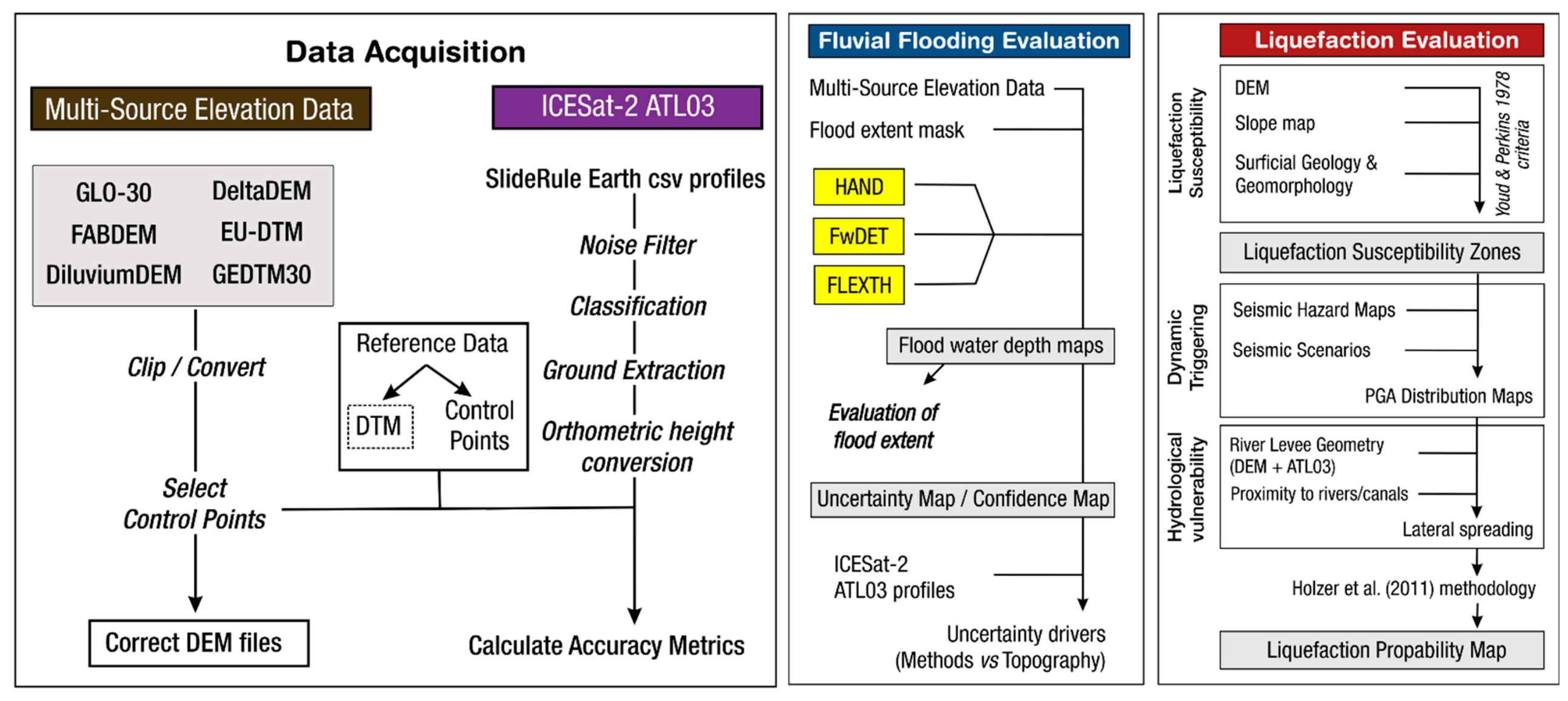
Our proposed process for hazard evaluation of coastal/estuarine Salt Ponds (DAFFLE), with a focus on river and canal levee protection, is split into three steps. Data from multiple global elevation datasets and ICESat-2 geolocated photon profiles are selected and processed within the boundaries of the study area (Figure 4).
Fluvial flooding evaluation follows, through water depth modeling for selected flood events. Then a liquefaction evaluation is performed with mapping of liquefaction through surficial geology and terrain; simplified liquefaction probability maps can be produced for existing Seismic Hazard Assessment products or multiple seismic scenarios.
The selection of data and methods used in this workflow are proposed to counter the prospect of data-scarcity in areas around the globe [17,18], and to employ tools and techniques that do not require special expertise. DAFFLE methodology does not replace a detailed site study, where more specific locally available data might be used.
Figure 4.
DAFFLE-Flowchart of data acquisition and geohazard evaluation for fluvial flooding and liquefaction in coastal/estuarine Salt Ponds [19].
3.1. Digital Elevation Models
The selection of an appropriate digital elevation model (DEM) represents a fundamental step for the proposed methodological framework (Figure 4). DEM selection was based on two major criteria:
- (a)
- spatial coverage, with preference given to freely available datasets offering global or regional coverage in order to address the limited availability of elevation data in many parts of the world;
- (b)
- spatial resolution, whereby only DEMs with a spatial resolution of 30 m (1 arc-second) were considered. This resolution was deemed the most suitable compromise between data availability and topographic detail, enabling the representation of relatively small-scale geomorphological and hydraulic features, including river levees, artificial canals, and flood protection infrastructure [20,21]. While 3 arc-second (90 m) or coarser resolution raster hydrography datasets, such as MERIT DEM [22], are popular for basin and regional scale hydrologic and flood hazard analyses [23,24], we consider this resolution as insufficient for local-scale studies.
To this end, five of the most recent global digital elevation models (DEMs) currently available were selected and compared: COP30, FABDEM, DeltaDTM, DliluviumDEM, EU-DTM, and GEDTM30. A summary of the selected DEMs and their main features is provided in Table 2.
Table 2.
Digital elevation models selected and their main features.
FABDEM (Forests And Buildings removed DEM) uses machine learning for the removal of trees and buildings in the Copernicus DEM [26]. The result is a global elevation model that improves upon COP30, especially for flood and hydrologic modelling.
DeltaDTM, a global coastal digital terrain model [28] makes use of space-borne lidar missions (ICESat-2 and GEDI) for co-registration and removal of non-ground points in Copernicus DEM. While DeltaDTM is available only for coastal areas, we consider that its coverage is sufficient for Salt Ponds which are found mainly in coastal areas.
DiluviumDEM [30,31] is a DEM with focus on accurate representation and enhancing accuracy of global coastal topography. DiluviumDEM (‘Flood’ in Latin) makes use of deep learning algorithms (LightGBM regression model) and high-resolution local datasets (Lidar) for the improvement of Copernicus DEM.
The EU-DTM (digital terrain model for Continental Europe—[33]) also makes use of space borne lidar data (GEDI, ICESat-2) trained together with a multitude of input layers (satellite land, forest and surface water cover; MERIT DEM; Copernicus DEM; ALOS AW3D30; EU DEM). EU-DTM might contain residual forest canopy points and has not been hydrologically corrected.
GEDTM30 (global ensemble digital terrain model) at 1 arc-second resolution is the last entry in the DEM list [34]. GEDTM30 also merges multiple global DEMs, space borne lidar and land cover data and produces an open ensemble digital terrain model, together with multiple terrain variables, with focus on terrain analysis and improvement of high-elevation areas.
The COP30 (GLO-30) is a Copernicus Digital Surface Model [25] derived from TanDEM-X data acquired between 2011 and 2015, with the primary objective of producing a high-resolution global elevation dataset [35]. It represents the Earth’s surface, including buildings, infrastructure, and vegetation. The dataset was further post-processed by flattening water bodies to ensure hydrological consistency and improve the representation of river flow.
The COP30 DEM exhibits superior performance compared to other global DEMs in terms of (a) spatial coverage, (b) spatial detail, as the dataset is derived from resampling an original 0.4 arc-second resolution product, and (c) vertical accuracy [36,37,38]. According to its specifications, COP30 achieves an expected vertical accuracy of approximately 2 m in smooth terrain with slopes < 20% on a global scale [35,39,40,41]. Furthermore, Huang and Yu [42], by quantitatively analyzing the variation of elevation errors as a function of slope and comparing the accuracy of different DEMs, suggests that COP30 may be more suitable for gentle slope regions (slope < 6°).
In addition, for comparison purposes, a local model was employed, namely the highest-resolution open-access digital elevation model available, the 5 m DTM available for the Emilia-Romagna Region. However, examination of this DTM in the study area reveals an inconsistency in the source material and the final product; there are patches with fine detail originating from lidar aerial survey DTMs, and patches with low-resolution data, interpolated from topographic maps (Figure S2).
Therefore, we did not use this DTM product as a reference dataset due to spatial inconsistencies, variable horizontal resolution, and artifacts created between different patches. We alternately used control points extracted from the DBTR (DataBase Topografico Regionale; [43]) digital maps in 1:25,000 scale, surveyed between 2003 and 2012. The comparison of the DEMs analyzed is presented in Section 3.3.
3.2. ICESat-2 Data
Since September 2018, the Ice, Cloud, and Land Elevation Satellite—2 (ICESat-2) mission provides space borne lidar-derived global geolocated photons through the ATLAS (Advance Topographic Laser Altimeter System) sensor [44,45,46]. From an orbit of ~500 km, the ATLAS sensor transmits laser scans split into three pairs of six individual beams with a total width of 6 km. Each pulse returns geolocated photons at ~0.7 m intervals and a vertical accuracy of ~10 cm.
For the purpose of this study, we use ATL03 data produced by the ICESat-2 mission. Ideal for survey profiling of large areas, ATL03 products offer geolocated ellipsoidal heights for each photon event. Height information is corrected for several geophysical parameters that affect photon routing and properties (e.g., atmospheric refraction, tides) and classified either as likely signal photons or likely background noise [47]. ICESat-2 profiles can serve as a manual inspection of flood barriers (embankments, levees) and identification of riverbeds, canals, and ditches with significant depth and width (Figure 5). This approach can improve the limited capability of DEMs at levee and canal detection.
Figure 5.
Example of ICESat-2 ATL03 profile across the study area (for the position see Figure 1). Geolocated photons are colored based on classification. ICESat-2 ground profiles can identify and remove areas with non-ground cover, such as forest patches and buildings, and visualize small levees/embankments and river/canal shapes. Photon original ellipsoid heights are transformed into EGM2008 orthometric heights.
ICESat-2 profile data have been successfully applied to regional fluvial and flood studies [48,49,50,51,52,53,54].
3.3. Evaluation of Horizontal and Vertical Accuracy of Elevation Data
All DEM files were projected into the same grid and reference system (UTM 32N WGS84) and EGM2008 geoid for height. Differences between the DEM files in comparison with the COP30 in the study area are provided in Figure 6.
Figure 6.
Selected DEM files (a), comparison with COP30 in map view (b), and scatterplot (c). Error distribution and vertical residuals for each DEM file in comparison with the reference control points (d), and after correcting systematic bias shift (e). Correlation matrices for calibrated elevation after bias removal and residual correlation between DEM files (f).
A comparison of the results (Figure 6b) shows a general convergence between DEMs, with local variations attributed to various conditions of non-ground object removal. Different approaches for water masking are also evident. Scatterplots (Figure 6c) show that all tested DEMs have a strong correlation with the reference COP30 dataset across most elevation ranges. Visible scattering and departure from the 1:1 line at the bottom indicates that local topographic variations, vegetation, or structural artifacts cause the models to deviate from one another in flat coastal plains. Scattering and deviation at the higher parts of the scatterplots is a sign of more efficient non-ground object removal for these DEMs [55].
To assess how terrain elevation influences topographic errors across the different DEM datasets, the study examines vertical accuracy through a two-fold approach:
- (a)
- utilizing key statistical metrics, including mean error (bias), root mean square error (RMSE), the correlation coefficient (R2), median normalized absolute deviation (MAD), and linear error at 90% confidence;
- (b)
- employing ground control points (CPs) extracted from the DBTR as a reference baseline. Original number of CPs was reduced by stratified selection with spatial thinning, with a final number of 60 CPs from a total of 9821 (Figure S4).
Comparing CP with each DEM reveals a systematic error bias, as displayed in Figure 6d. COP-30 has the largest distribution of vertical residuals, as expected due to the significant presence of non-ground objects.
EU-DTM has a distinctively larger negative shift than the rest of the DEMs. This bias can be attributed to the temporal change in surface elevation between data acquisition, local residuals of non-ground objects, and errors from transformation to EGM2008 from the original surveyed data. Bias shift was calculated independently for every DEM file and then applied to the raster file correction. The final results (i.e., post-shift correction) display sufficient accuracy, with a mean RMSE of ~1 m (Figure 6e, Table 3). The final error distribution shows an overall convergence near zero (Figure 6e). DEM files with bias shift correction are then ingested into the workflow.
Table 3.
Correction of systematic bias in DEM files using control points.
The final correlation matrix (green in Figure 6f) shows near-perfect correlation values (>0.98) between the calibrated elevation values of almost all DEMs, an indication of good coverage of topographic features and elevation ranges. Even after calibration, the errors in the residual correlation matrix (red in Figure 6f) remain moderately to highly correlated (r ≈ 0.73 to 0.83) across the different datasets. The presence of systemic error patterns, inherited from the shared base data in multiple DEMs, can explain this correlation.
Query, downloading and pre-processing of ICESat-2 profiles of geolocated photons is performed by employing SlideRule Earth Python client and icepyx Python code (Python version 3.10). All available profiles (2018 to 2025) over the assigned area of interest were queried and downloaded as separate csv files. A total of 159 ATL03 profiles (including both strong and weak pulses) were extracted over the study area, consisting of 5,540,334 geolocated photons (Table S1). Each profile was then filtered for noise photon removal with the DBSCAN algorithm [56], classified and ground points were extracted. Ground extraction was tested with different approaches such as moving window and median percentile filtering. We selected the adoption of the 40th percentile extraction as it was a better fit for our data, balancing non-ground point residuals and sufficient uplifting of ground surface in comparison with DEM and control point reference heights (Figure S3).
Ellipsoidal heights for each photon were transformed into orthometric EGM2008 elevations, for consistency with the DEM files. ATL03 profiles were also checked against the control point dataset, and final residuals for ground points were found to be within an RMSE of 0.2 to 1.0 m (Figure S4).
3.4. Fluvial Flood Evaluation
For the evaluation of fluvial flooding in the vicinity of the Salt Pond, we selected three geomorphic flood methods that model flood water depth:
- (a)
- Height Above Nearest Drainage—HAND [57,58,59]. For the HAND implementation, we used the published code by CSIRO Australia [60]. HAND is a terrain model that normalizes topography along drainage networks to map soil water environments;
- (b)
- Floodwater Depth Estimation Tool (FwDET v2) for improved remote sensing analysis of coastal flooding proposed by Cohen et al. 2019 [58]. FwDET calculates water depth by subtracting the calculated floodwater elevation (above mean sea level) from topographic elevation at each grid cell within the flooded domain. Main output characteristics include a raster-based water depth map and improved boundary handling capabilities [61];
- (c)
- FLEXTH—Flood Extent Enhancement and Water Depth Estimation Tool for satellite-based inundation maps [62]. FLEXTH combines flood maps with topographic data (DTM) to extend the flood delineation into no-data areas, where floodwater is expected due to topography, as well as to estimate water levels and water depths. Main output characteristics include water depth and water level raster maps, explicit interpolation into unmapped gap, RMSE about 0.18 m [61].
The rationale behind this choice lies in the ability of estimating floodwater depths associated with inundation events directly from digital elevation models [63]. In contrast, hydrodynamic models typically require a large amount of hydraulic input data, which is often unavailable for the study area. Furthermore, the use of three different geomorphic methods enables a comparative analysis, reducing the model-specific uncertainties and improving the reliability of flood depth estimates in this highly sensitive coastal-transition environment [64].
While HAND and FwDET v2 primarily focus on cross-sectional or drainage-network-based terrain scaling, FLEXTH introduces a specialized boundary-propagation routine. This feature makes it particularly well suited for addressing fragmented flood extents and artificial “NoData” gaps commonly encountered in highly engineered coastal environments.
While other geomorphic based flood hazard methods are widely employed, such as the Geomorphic Flood Index—GFI [65,66] and Teng Vaze Dutta—TVD [67,68,69], we did not integrate them as they usually require a greater extent of study area that includes the watershed basin (GFI) or might not work well with fragmented flood water extent as they require local slope adjustments (TVD). A flood extent mask or local flood water depth reference dataset can be selected within recent significant flooding events. Flood water depths were modelled for each different input DEM using the 2023 Emilia-Romagna flood extent as a mask. Since DeltaDTM had the Cervia Salt Pan masked with no data values, we added an interpolated filled DEM version, resulting in an output of 3 × 21 raster maps. Flood water depth maps can greatly enhance the evaluation of flooding, provide a more in-depth understanding of flood water flow and accumulation, and highlight areas where significant flood protection projects should be focused.
3.5. Liquefaction Evaluation
For a simplified approach to liquefaction in the study area, we apply the criteria of Youd and Perkins [70]. Although geotechnical site investigations are crucial for site-specific performance, a regional approach can be based on the surficial geology using lithology as a proxy.
Ground investigation data (boreholes, tests, loggings, samples) can be very scarce if not absent in most regions from a global perspective. Substituting ground investigations with geological and geomorphological data is a viable alternate as there is a very strong correlation with liquefaction susceptibility and manifestations from earthquake events [19,71,72,73,74].
Surficial geological and geomorphological formations are assigned different classes of liquefaction susceptibility based on their age, depositional environment, and lithology.
In the absence of detailed surficial geological maps and/or geomorphological maps in an area, mapping of these features can be performed using digital elevation data in combination with historical and recent imagery (e.g., [72,74,75]. Recent or inherited fluvial and coastal features, such as river meanders or abandoned channels, coastal sand dune ridges, etc., can be identified even in medium resolution digital elevation models and satellite imagery. Slope gradient maps can increase the identification of fluvial and coastal landforms in areas with gentle relief, such as coastal plains and deltas.
Based on these criteria, we assign a susceptibility class in every mapped recent formation of the Pleistocene and Holocene age. Water depth is also an important factor for assessing liquefaction susceptibility, with a broad consideration that areas with a water table depth less than 2–5 m are susceptible to earthquake triggered liquefaction and lateral spreading. Liquefaction and lateral spreading are also inherently related to localized strong ground motion and earthquake occurrence.
In order to produce a liquefaction probability map, without resorting to detailed seismic hazard analysis and earthquake geotechnical models, we adopted the simplified empirical approach proposed by Holzer et al. [19]. This approach is based on statistically derived liquefaction probability curves obtained from a large database of cone penetration tests (CPT) and is specifically designed for regional-scale hazard assessments.
As indicated by Holzer et al. [19], these curves are intended for use in transforming surficial geologic maps into probabilistic liquefaction hazard maps in situations where site-specific geotechnical data are not available. The probabilistic relationships are conditioned on seismic parameters such as earthquake magnitude and peak ground acceleration and are derived from complementary cumulative frequency distributions of the liquefaction potential index (LPI).
Within this framework, generic curves provide a first-order, statistically based approximation of the liquefaction hazard and are widely employed in regional-scale hazard mapping and zoning applications, particularly under conditions of limited subsurface information.
Using the input data as classified using Youd and Perkins [70] criteria and earthquake/strong motion values (magnitude/peak ground acceleration PGA), Holzer et al. [19] developed a set of variables that can be inserted into the empirical relationship for liquefaction probability.
Two sets of constants a, b, and c are provided, for water table depths of 1.5 m and 5 m, used for the logistic regression of multiple ground investigation data for each deposit type. From multiple measurements of the water table in the shallow aquifer of the study area, we estimate a mean water table depth of ~1 m (assuming a constant value throughout the entire domain), thus adopting the first set of constants from Holzer et al. [19].
The equation for probability of liquefaction is the following:
where a, b, and c are variables computed for the logistic regression of each class, PGA is the peak ground acceleration, and MSF is the magnitude scaling factor as defined by Youd et al. [76].
P = a/(1 + ((PGA/MSF)/b))c,
Assuming a data-scarce study area, we used the latest version of Global Earthquake Model Foundation (GEM, [77]) global seismic hazard grid for the PGA value (0.2 g for a 475-year return period), transformed with the appropriate amplification factor from rock to soil value [78].
The Italian Archive of Historical Earthquake Data, ASMI [79] was used to identify a reference earthquake for our study area. The area of Cervia has experienced the maximum recorded macroseismic intensity of 8 in three earthquakes; Mw 5.6 14 April 1672, Mw 5.75 17 March 1875, and Mw 5.82 17 May 1916 [80]. Based on these historical data, a reference earthquake of magnitude Mw 5.8 was used as an input for the empirical relationships.
4. Results
4.1. Fluvial Flooding
A comparison of the flood water depths modelled by each method is displayed in Figure 7. The HAND method overestimates flood water depths while FwDET and FLEXTH perform better. Fragmented patches of flood water in this case study, and a lack of a defined fluvial valley (as in this area the Savio River levee forms the higher elevation ridge) contribute to the inadequate results of HAND.
Figure 7.
Results of flood water depth modelling using the 2023 flood extent dataset and DiluviumDEM: (a) HAND method; (b) FwDET; (c) FLEXTH; (d), (e) and (f) represent zoomed-in details of the HAND, FwDET, and FLEXTH results, respectively, for the area outlined by the white rectangle shown in the corresponding panels (a), (b), and (c).
FwDET and especially FLEXTH take into account flood water flow connectivity and local water level variations. For a comparison of the FwDET and FLEXTH results, we discarded the HAND flood water depth maps due to their overprediction for our case study. We produced cumulative uncertainty (standard deviation in meters) and confidence (agreement) maps (Figure 8).
Figure 8.
Cross-validation of flood water depth modelling excluding HAND results: (a) confidence map—percentage of agreement; (b) standard deviation (σ) in meters. Location of profiles 1 and 2 of Figure 9 is also shown.
Agreement of water depths maps is in a high percentage around the Cervia Salt Pond. Uncertainty is also low for the Salt Pond, with only few spots exhibiting high σ values. On investigating the uncertainty driver in water depth modeling, correlation analysis shows that topography variance acts as the dominant influence on uncertainty compared to the algorithm used (Figures S5 and S6).
As the topography is the main factor leading to differences in water depth maps, we used ICESat-2 geolocated photon profiles for examination of areas with low agreement and high uncertainty [81]. Using all the classified ATL03 profiles, we overlayed those with the uncertainty and confidence maps. We rendered all 159 profiles, with geolocated photons colored for thresholds of >0.8 m of uncertainty and <75% confidence.
Examination of the profiles (Figure 9) reveal that most areas of water depth variance are related to residuals of non-ground objects (tree canopy, buildings). Through this process, ICESat-2 profiles can evaluate the local shortcomings of DEMs employed for flood water depth modelling and can highlight areas where DEMs can be improved.
Figure 9.
Examples of ICESat-2 profiles with geolocated photons rendered in color above areas with low confidence and high uncertainty of water depth maps. Location of profiles is shown in Figure 8.
4.2. Liquefaction and Lateral Spreading
Liquefaction assessment can be divided into three main stages; (a) liquefaction susceptibility mapping, (b) dynamic triggering for single or multiple earthquake scenarios and strong ground motion effect, and (c) hydrologic vulnerability (Figure 4). Final products are the liquefaction probability maps and zonation of areas prone to lateral spreading (proximity to river levees, canals).
Liquefaction susceptibility map based on the criteria of Youd and Perkins [70] classifies the Savio River and the coastal dune ridges as zones of high liquefaction susceptibility (Figure 10).
Figure 10.
Results of earthquake triggered liquefaction evaluation: (a) liquefaction susceptibility classes based on mapped geological units; (b) liquefaction probability map for a scenario earthquake of Mw 5.8/PGA = 0.2 g, based on the methodology by Holzer et al. [19].
The very high susceptibility class is restricted by the published geological map to a small section of the Savio River, but it is considered to be of a greater extent, covering a narrow zone along the natural levee and the meandering course. This very high susceptibility zone could be augmented by manual mapping of surficial geology and geomorphological features. Low elevation areas behind the coastal ridges are considered of medium liquefaction susceptibility, but spatial lithological uncertainty and probable increased clay content might restrict triggered liquefaction and lateral spreading only locally.
The liquefaction probability map, based on the seismic scenario described in Section 3.4, also shows medium-to-high probability around the Savio River and the coastal section. The Savio River course area is of more interest in our study as it could result in levee liquefaction and subsequent failure, in contrast with the coastal sand dune ridges where failures will not affect water flow into the Salt Pond low. High and very high susceptibility zoning and the liquefaction probability map define the areas that are under danger of triggering lateral spreading of the natural and artificial levees of the Savio River, leading to a probable breach and overflow towards the Cervia Salt Pond.
5. Discussion
5.1. Levee Failure and Salt Pond Flooding
Our methodology highlights the probable source and effects of levee failure and flooding for the Cervia Salt Pond. The most important source of potential flooding of the Salt Pond is a failure of the Savio River’s natural or artificial levee along its course running west and north of the pond. Topographic gradient and flood water depth mapping reveal a concentration of surface water flow towards the low basin of the pond (Figure 11).
Figure 11.
Topographic profiles (①, ②, ③) across the Cervia Salt Pond and the Savio River showing a clear gradient towards the Cervia Salt Pond.
Flood water from a potential breach or overflow along the Savio River course south of Castiglione will be captured and diverted by the Canale Emiliano Romagnolo (CER) and the irrigation canal (Canale) to the south of the Cervia Salt Pond (Figure 11). The flood extent and the modelled flood water depth maps of the May 2023 flood event also confirm this lack of significant water inflow from the west and south of the Salt Pond. A fluvial flooding hazard from the coastal sand ridges east of the pond is also considered as low or absent.
Levee failure could be triggered by abnormal water flow during extreme rainfall events [16] or liquefaction/lateral spreading triggered by a moderate/strong earthquake [82,83,84]. Potential breach location could be identified along the course of the river natural levee, examining spots where artificial embankment and levees are degraded and where fluvial geomorphology might indicate probable change in water flow dynamics.
We consider the May 2023 breach location north of Castiglione (Figure 3) as a candidate location also of future levee failures. This location is a spot where the Savio River makes an abrupt path change with a sharp turn from the northeast direction to the northwest. The reasons for this river anomaly is believed to have originated as a consequence of the extensive human modification and alteration of the course back in the early 19th century (or earlier) as evident from historical topographic maps (Figure 12). This location also coincides with the termination of the preserved natural course of the Savio River and the beginning of the modified course up to the Adriatic Sea coast. The human modification of the river course is also clear in historical and modern maps of the area, especially the geological map sheet of Forli-Cervia (Figure 12b) where relict meanders are preserved in the landscape.
Figure 12.
(a) Relation of the 2023 levee breach (arrow) with modification of the Savio River course downstream of this bend location. (b) Geological map showing the persisting evidence of paleo-meanders. (c) The 1851 topographic map showing that the Savio course had already been modified and straightened in its final reach from the mid XIX century.
In this regard, as reported by the local chronicler Giuliano Fantaguzzi in 1502 (Fantaguzzi, Caos, cit., vol. I, p. 27; [85]), the area surrounding the Savio River near Martorano (approximately 9 km southwest of Castiglione) was frequently affected by severe flood events. Cesare Borgia therefore summoned Leonardo da Vinci, who, upon inspecting the hydraulic works being carried out along the Savio River for the protection of the settlement, advised the Duke against the straightening of the river course, in order to avoid increasing the flow velocity and the consequent erosion processes.
The 2023 breach location is found near the historical Canale di Duca (Duke’s canal). The Canal of the Duke of Altemps was constructed in the early 10th century AD but was later abandoned. Along the canal we can find today the Bosco del Duca d’Altemps, a 1 km long forest stretch of trees up to 30 m in height. During May 2023, this abandoned canal and forest patch served as a southern barrier to the flood water in its attempt to flow towards the Cervia Salt pond (Figure 3b,c).
5.2. Evaluation and Proposed Protection Measures
Our methodology highlights the probable source and effects of levee failure and flooding for the Cervia Salt Pond. As previously described, we consider that a potential levee failure of the Savio River due to increased water flow and/or an earthquake is the most probable cause of flooding in the Cervia Salt Pond. A summary of the evaluation results for the study area is shown in Figure 13. Two areas of relatively high and very high hazard are depicted around the course and natural levee of the Savio River.
Figure 13.
Relative hazard evaluation and flooding origin for the Cervia Salt Pond study area. Line pattern shows liquefaction susceptibility along the Savio river levee. Blue arrows show possible flood water paths towards the topographic low. The black arrows indicate the sections of the Savio River where a potential levee breach could either cause or prevent flooding of the salt pond.
We delineate two areas of elevated hazard and the future focus on the planning of mitigation measures along the Savio River:
- (a)
- The northern section, from Castiglione up to the coastal sand ridges, is considered of relatively ‘very high hazard’, as this reach has experienced levee breaches in the past (e.g., May 2023), and water overflow will flood the Salt Pond topographic low with minimal obstacles along its path. This section also has increased levee breach potential due to the river course geometry and inherited geomorphological conditions;
- (b)
- The southern section, upstream of Castiglione, is considered of ‘high hazard’ due to conditions favoring a potential levee failure and overflow (high liquefaction susceptibility, water toppling, and overflow behavior). As concerns the Cervia Salt Pond, this section is considered of relatively lower hazard as far as the potential overflow of flood water will be largely captured and/or diverted away from the Salt Pond due to the presence of the large Canale Emiliano Romagnolo (CER) and a secondary major canal (Figure 12).
Following the results and analyses of potential hazard and local conditions, we propose focus areas for future planning of mitigation and protection measures. Potential flooding of the Cervia Salt Pond can be mitigated by either flood protection and flood water prevention along the Savio River or by enhancing flood protection measures within and around the Salt Pond. These could be represented by the construction of new embankments or an elevation of the existing ones all around the Salt Pond, and/or enlarging the water diversion canals such as the District Canal that runs along 14 km of the Salt Pond perimeter and diverts water into the coast of Cervia. The latter option is likely the less optimal of being disruptive to the environment of the protected natural site of the Cervia Salt Pond. Thus, we propose that flood prevention and mitigation projects should be focused on the Savio River course and its natural levee. These could be the strengthening and repair of existing artificial levees and embankments, the removal of sediment fillings, and the construction of new flood protection embankments and ditches.
Fluvial flood mitigation measures for Salt Ponds can include structural protection and engineering methods:
- dike and levee reinforcement by increasing the height of existing dikes as a defense against sea level rise and flood water;
- installation of floodgates, seawalls, and barrages to control water flow and prevent excessive saltwater intrusion into production areas;
- bypass and diversion channels.
An alternative that is more environmentally friendly could be the application of nature-based solutions (NBS) that might include salt marsh construction or restoration, mangrove barriers, and development of wetland buffers around the structure. Considering that the area of the Cervia Salt Pond is a protected environmental site, mitigation, infrastructure, or NBS projects involving land transformation or modification may be difficult to implement, as they are subject to significant regulatory and ecological constraints in order to avoid potential negative impacts on biodiversity, natural habitats, and the ecological balance of the area.
5.3. SWOT Analysis of the DAFFLE Methodological Approach
DAFFLE provides a first-order assessment of the intrinsic vulnerability of coastal productive systems, both existing and planned. Accordingly, it is intended to operate as a decision-support tool for stakeholders involved in spatial planning, risk assessment, and territorial management. It is nevertheless important to emphasize that DAFFLE is not conceived as a substitute for detailed geotechnical, hydrological, and hydraulic analyses. Such analyses, based on dedicated field investigations and advanced numerical models, remain essential in subsequent design, verification, and risk mitigation phases.
The SWOT analysis of the DAFFLE methodological approach can be effectively implemented by identifying, analyzing, and categorizing the diverse internal and external factors that influence each of the four components: Strengths, Weaknesses, Opportunities, and Threats.
The main strengths of the DAFFLE approach can be summarized as follows:
- (a)
- simplicity and rapid applicability, minimizing the need for detailed site-specific data (e.g., geotechnical, hydraulic, hydrological, geological, and hydrogeological information);
- (b)
- global applicability, through the use of available, large-scale elevation datasets; to this end, Section 3 presents an analysis and comparison of different global digital elevation models (DEMs) and ICESat-2-derived elevation profiles, in order to identify solutions that provide the best trade-off between spatial resolution, geographic coverage, and reliability;
- (c)
- low operational costs, thanks to the use of freely accessible satellite-based datasets and simplified numerical formulations that require a limited number of input parameters;
- (d)
- reduced computational demand, as the methodology does not depend on high-performance computing resources or computationally intensive modelling framework requirement;
- (e)
- flexibility, as it can be adapted and/or integrated with other techniques to meet specific contexts and needs.
Despite these advantages, the methodology has several limitations:
- (a)
- DAFFLE is not intended to be universally applicable, and its performance may vary when applied to environmental and geomorphological settings that differ from those for which it was originally developed and calibrated;
- (b)
- furthermore, it should be considered a screening-level tool rather than a substitute for detailed geotechnical, hydrological, and hydraulic investigations;
- (c)
- the reliability of its results also depends on the quality, resolution, and availability of the input datasets.
Several opportunities exist for the further development of the methodology:
- (a)
- validation in different geographical and environmental contexts will enhance the robustness and transferability of the framework;
- (b)
- the increasing availability of high-resolution satellite products and global elevation datasets offers unique opportunities to refine and expand the methodology;
- (c)
- additional future applications could foster collaboration among hydrologists, geologists, hydrogeologists, engineers, and spatial planners, thereby promoting integrated approaches to risk assessment.
At the same time, it must be acknowledged that, the improper application of the methodological approach, as well as the use of unsuitable or inaccurate input data (e.g., reference magnitude, piezometric level, or geometric characteristics of surficial deposits, etc.), may compromise the reliability of the assessment and potentially result in significant adverse consequences (threat).
6. Conclusions
Climate change, together with the high economic, landscape, and ecological value of coastal Salt Ponds, is making the development of effective strategies for their sustainable management and protection increasingly urgent. These systems are highly vulnerable environments, where the interaction between fluvial processes, coastal dynamics, and human intervention can significantly amplify exposure to natural hazards.
In this context, this paper presents a simplified multi-hazard methodological framework (DAFFLE) for assessing fluvial flooding and liquefaction hazards in natural coastal environments used for salt production. The approach integrates heterogeneous and widely available datasets, including global digital elevation models, high-resolution topographic information derived from the ICESat-2 mission, flood inundation estimation, and a simplified assessment of liquefaction susceptibility based on surface geological and geomorphological parameters. This integration enables the development of a coherent and transferable analytical framework applicable even in data-scarce regions where detailed geotechnical investigations are not available.
Although intentionally simplified, the proposed method (DAFFLE) allows first-order assessments of hazard conditions in coastal and estuarine Salt Pond systems, providing a useful basis for comparative analyses across regional to global scales. Rather than replacing detailed site-specific investigations, the framework is intended as a preliminary screening tool to support better territorial planning and risk management, ultimately contributing to more effective long-term management and protection of coastal Salt Pond systems.
In particular, the application of the method to the Cervia Salt Pond in Emilia-Romagna (Italy) allowed the identification of the main fluvial sectors responsible for the system’s hydraulic exposure. Topographic analysis combined with flood modelling reveals a strong convergence of surface runoff toward the Salt Pond depression, which acts as the main hydraulic sink during extreme events. The May 2023 flood event further confirms the system’s vulnerability, highlighting the potential for levee failure and the limited effectiveness of existing flood protection structures under extreme conditions.
The results also emphasize the importance of integrating fluvial and seismic processes within a unified analytical framework, particularly in low-lying coastal environments where overlapping hazards may generate complex, non-linear risk scenarios. In such settings, the interaction between hydraulic instability and liquefaction susceptibility can significantly amplify the overall system vulnerability.
Future investigations could include the incorporation of high-resolution geotechnical datasets, the use of advanced hydrodynamic simulations, and the modelling of multi-temporal climate-driven scenarios. These improvements would enhance vulnerability estimation and increase the predictive capability of the framework, ultimately supporting more effective long-term management and protection of coastal Salt Pond systems.
Supplementary Materials
The following supporting information can be downloaded at: https://www.mdpi.com/article/10.3390/environments13070400/s1, Figure S1: Comparison of the digital elevation models (DEMs) selected as input data; Figure S2: Comparison of the 5 m digital terrain model (DTM) by Emilia-Romagna Region and Copernicus 30 DEM; Figure S3: Examples of ground extraction in an ICESat-2 profile, using different methods; median 10th percentile filtering (a), 40th percentile filtering (b), 510th percentile filtering (c); Figure S4: Total control points versus final selection of CPs. Correlation scatter plots with elevation for each DEM and control points; Figure S5: Flood water depth maps modelled with all three methods (HAND, FwDET and FLEXTH); Figure S6: Correlation matrix between different water depth models and uncertainty driver—method vs. elevation; Table S1: List of ICESat-2 ATL03 profiles accessed through SlideRuleEarth client.
Author Contributions
Conceptualization, D.R. and S.V.; methodology, D.R. and S.V.; software, S.V.; validation, D.R.; formal analysis, S.V.; investigation, D.R. and S.V.; resources, D.R.; data curation, S.V. and D.R.; writing—original draft preparation, D.R. and S.V.; writing—review and editing, D.R.; supervision, D.R.; project administration, D.R.; funding acquisition, D.R. All authors have read and agreed to the published version of the manuscript.
Funding
The research activities of S.V. are partially supported by bePrepARed project (Preparing, Adapting, Reconstructing: actions to promote climate change adaptation and risk disaster resilience in Italian and Croatian sensitive ecosystems; Project Number: E39G24000460007).
Data Availability Statement
The data presented in this study are available on request from the corresponding author due to privacy restrictions.
Acknowledgments
We thank the staff of the former Emilia-Romagna Regional Reconstruction Agency, the Regional Agency for Territorial Safety and Civil Protection of the Emilia-Romagna Region, and the Cervia Salt Pond Park for the valuable collaboration. We also thank the anonymous reviewers for their constructive comments, which improved the manuscript.
Conflicts of Interest
The authors declare no conflicts of interest.
Abbreviations
The following abbreviations are used in this manuscript:
| AGEA | Agenzia per le Erogazioni in Agricoltura, Italia |
| ALOS AW3D30 | Advanced Land Observing Satellite (ALOS) World 3D—30 m |
| ATLAS | Advance Topographic Laser Altimeter System—sensor mounted on ICESat-2 satellite |
| CARG | Geological CARtography project—Istituto Superiore per la Protezione e la Ricerca Ambientale |
| CER | Canale Emiliano Romagnolo |
| COP30 | Copernicus 30 m digital elevation model |
| DBTR | DataBase Topografico Regionale—Italy |
| DeltaDTM | Global coastal digital terrain model |
| DEM | Digital elevation model |
| DTM | Digital terrain model |
| EGM2008 | Earth Gravitational Model 2008 |
| EU DEM | European Union digital elevation model |
| EU-DTM | Continental Europe digital terrain model |
| FABDEM | Forests And Buildings removed digital elevation model |
| FLEXTH | Flood Extent Enhancement and Water Depth Estimation Tool |
| FwDET | Floodwater Depth Estimation Tool |
| GEDI | Global Ecosystem Dynamics Investigation—Lidar sensor mounted on the International Space Station |
| GEDTM30 | Global ensemble digital terrain model 30 m |
| GEM | Global Earthquake Model Foundation |
| GFI | Geomorphic Flood Index |
| GLO-30 | Global 30-m digital elevation model (Copernicus digital elevation model) |
| HAND | Height Above Nearest Drainage |
| ICESat-2 | Ice, Cloud, and Land Elevation Satellite-2 |
| LightGBM | Light Gradient-Boosting Machine—open-source distributed gradient-boosting framework for machine learning |
| MAD | Median normalized absolute deviation |
| MERIT DEM | Multi-Error-Removed Improved-Terrain Digital Elevation Model |
| MSF | Magnitude scaling factor |
| NBS | Nature-based solutions |
| PGA | Peak ground acceleration |
| RMSE | Root mean square error |
| SWOT | Strengths, Weaknesses, Opportunities, and Threats analysis |
| TanDEM-X | TerraSAR-X add-on for Digital Elevation Measurement—a German twin satellite mission using interferometric synthetic aperture radar |
| TVD | Teng Vaze Dutta—geomorphic flood algorithm |
References
- Horden, P.; Purcell, N. The Corrupting Sea: A Study of Mediterranean History; Blackwell Publishing: Oxford, UK, 2000; p. 761. [Google Scholar]
- Bevacqua, E.; Maraun, D.; Vousdoukas, M.I.; Voukouvalas, E.; Vrac, M.; Mentaschi, L.; Widmann, M. Higher probability of compound flooding from precipitation and storm surge in Europe under anthropogenic climate change. Sci. Adv. 2019, 5, eaaw5531. [Google Scholar] [CrossRef] [Scilit]
- Harrison, L.M.; Coulthard, T.J.; Robins, P.E.; Lewis, M.J. Sensitivity of estuaries to compound flooding. Estuaries Coasts 2021, 45, 1250–1269. [Google Scholar] [CrossRef] [Scilit]
- Meslard, F.; Balouin, Y.; Robin, N.; Bourrin, F. Assessing the Role of Extreme Mediterranean Events on Coastal River Outlet Dynamics. Water 2022, 14, 2463. [Google Scholar] [CrossRef] [Scilit]
- Nirwansyah, A.W.; Braun, B. Mapping Impact of Tidal Flooding on Solar Salt Farming in Northern Java using a Hydrodynamic Model. ISPRS Int. J. Geo-Inf. 2019, 8, 451. [Google Scholar] [CrossRef] [Scilit]
- Nirwansyah, A.W.; Braun, B. Assessing the degree of tidal flood damage to salt harvesting landscape using synthetic approach and GIS—Case study: Cirebon, West Java. Int. J. Disaster Risk Reduct. 2021, 55, 102099. [Google Scholar] [CrossRef] [Scilit]
- Nirwansyah, A.W.; Braun, B. Tidal flood risk on salt farming: Evaluation of post events in the northern part of Java using a parametric approach. Geosciences 2021, 11, 420. [Google Scholar] [CrossRef] [Scilit]
- Ding, M.; Lin, P.; Gao, S.; Wang, J.; Zeng, Z.; Zheng, K.; Zhou, X.; Yamazaki, D.; Gao, Y.; Liu, Y. Reversal of the levee effect towards sustainable floodplain management. Nat. Sustain. 2023, 6, 1578–1586. [Google Scholar] [CrossRef] [Scilit]
- Maranzoni, A.; D’Oria, M.; Mazzoleni, M. Probabilistic flood hazard mapping considering multiple levee breaches. Water Resour. Res. 2022, 58, e2021WR030874. [Google Scholar] [CrossRef] [Scilit]
- Selmi, M.; Hamdi, Y.; Moiriat, D. Multi-Hazard assessment of a flood protection levee. Atmosphere 2022, 13, 1741. [Google Scholar] [CrossRef] [Scilit]
- Mainguenaud, F.; Peyras, L.; Khan, U.T.; Carvajal, C.; Sharma, J.; Beullac, B. A probabilistic approach to levee reliability based on sliding, backward erosion and overflowing mechanisms: Application to an inspired Canadian case study. J. Flood Risk Manag. 2023, 16, e12921. [Google Scholar] [CrossRef] [Scilit]
- Golin, A.S.; Campos, H.R.P.; Ochoa, C.G.; Dávila, C.F.; Vives, L.S. Assessing open-access digital elevation models for hydrological applications in a large scale plain: Drainage networks, shallow water bodies and vertical accuracy. Earth Surf. Processes Landf. 2024, 49, 5269–5283. [Google Scholar] [CrossRef] [Scilit]
- ISPRA—Servizio Geologico d’Italia. Carta Geologica d’Italia alla Scala 1:50.000, Foglio 240-241 Forlì-Cervia; ISPRA—Servizio Geologico d’Italia: Rome, Italy, 2005; Available online: https://progetto-carg.isprambiente.it/cartografiaCARG/index.php?source=cartageologica®ione=Emilia-Romagna&foglio=240-241 (accessed on 31 October 2025).
- ISPRA-Servizio Geologico d’Italia. Note Illustrative della Carta Geologica d’Italia alla Scala 1:50.000, F240-241 Forlì-Cervia; ISPRA-Servizio Geologico d’Italia: Rome, Italy, 2005; Available online: https://progetto-carg.isprambiente.it/cartografiaCARG/index.php?source=cartageologica®ione=Emilia-Romagna&foglio=240-241 (accessed on 31 October 2025).
- Dorrington, J.; Wenta, M.; Grazzini, F.; Magnusson, L.; Vitart, F.; Grams, C.M. Precursors and pathways: Dynamically informed extreme event forecasting demonstrated on the historic Emilia-Romagna 2023 flood. Nat. Hazards Earth Syst. Sci. 2024, 24, 2995–3012. [Google Scholar] [CrossRef] [Scilit]
- Arrighi, C.; Domeneghetti, A. Brief communication: On the environmental impacts of the 2023 floods in Emilia-Romagna (Italy). Nat. Hazards Earth Syst. Sci. 2024, 24, 673–679. [Google Scholar] [CrossRef] [Scilit]
- Samela, C.; Troy, T.J.; Manfreda, S. Geomorphic classifiers for flood-prone areas delineation for data-scarce environments. Adv. Water Resour. 2017, 102, 13–28. [Google Scholar] [CrossRef] [Scilit]
- Peña, F.; Nardi, F.; Melesse, A.; Obeysekera, J. Assessing geomorphic floodplain models for large scale coarse resolution 2D flood modelling in data scarce regions. Geomorphology 2021, 389, 107841. [Google Scholar] [CrossRef] [Scilit]
- Holzer, T.L.; Noce, T.E.; Bennett, M.J. Liquefaction probability curves for surficial geologic deposits. Environ. Eng. Geosci. 2011, 17, 1–21. [Google Scholar] [CrossRef] [Scilit]
- Li, H.; Zhao, J.; Yan, B.; Yue, L.; Wang, L. Global DEMs vary from one to another: An evaluation of newly released Copernicus, NASA and AW3D30 DEM on selected terrains of China using ICESat-2 altimetry data. Int. J. Digit. Earth 2022, 15, 1149–1168. [Google Scholar] [CrossRef] [Scilit]
- Khanh, D.N.; Tsumura, Y.; Sasaki, O.; Shiraishi, K.; Akimoto, D.; Yamazaki, D.; Zhao, G.; Hirabayashi, Y. Mapping the World’s river Levees: A Hyper-Resolution levee database based on digital elevation models. Geophys. Res. Lett. 2025, 52, e2024GL114121. [Google Scholar] [CrossRef] [Scilit]
- Yamazaki, D.; Ikeshima, D.; Tawatari, R.; Yamaguchi, T.; O’Loughlin, F.; Neal, J.C.; Sampson, C.C.; Kanae, S.; Bates, P.D. A high-accuracy map of global terrain elevations. Geophys. Res. Lett. 2017, 44, 5844–5853. [Google Scholar] [CrossRef] [Scilit]
- Yamazaki, D.; Ikeshima, D.; Sosa, J.; Bates, P.D.; Allen, G.H.; Pavelsky, T.M. MERIT Hydro: A high-resolution global hydrography map based on latest topography dataset. Water Resour. Res. 2019, 55, 5053–5073. [Google Scholar] [CrossRef] [Scilit]
- Prusevich, A.A.; Lammers, R.B.; Glidden, S.J. Delineation of endorheic drainage basins in the MERIT-Plus dataset for 5 and 15 minute upscaled river networks. Sci. Data 2024, 11, 61. [Google Scholar] [CrossRef] [Scilit] [PubMed]
- European Space Agency; Airbus. Copernicus DEM; CDSE: Linthicum, MD, USA, 2022. [Google Scholar] [CrossRef] [Scilit]
- Hawker, L.; Uhe, P.; Paulo, L.; Sosa, J.; Savage, J.; Sampson, C.; Neal, J. A 30 m global map of elevation with forests and buildings removed. Environ. Res. Lett. 2022, 17, 024016. [Google Scholar] [CrossRef] [Scilit]
- Hawker, L.; Uhe, P.; Neal, J. FABDEM Updates-FABDEM V1-2; Zenodo (CERN European Organization for Nuclear Research): Geneva, Switzerland, 2023. [Google Scholar] [CrossRef]
- Pronk, M.; Hooijer, A.; Eilander, D.; Haag, A.; De Jong, T.; Vousdoukas, M.; Vernimmen, R.; Ledoux, H.; Eleveld, M. DeltaDTM: A global coastal digital terrain model. Sci. Data 2024, 11, 273. [Google Scholar] [CrossRef] [Scilit] [PubMed]
- Pronk, M. DeltaDTM v1.1: A Global Coastal Digital Terrain Model; 4TU.ResearchData: Delft, The Netherlands, 2024. [Google Scholar] [CrossRef]
- Dusseau, D.; Zobel, Z.; Schwalm, C.R. DiluviumDEM: Enhanced accuracy in global coastal digital elevation models. Remote Sens. Environ. 2023, 298, 113812. [Google Scholar] [CrossRef] [Scilit]
- Dusseau, D.; Zobel, Z.; Schwalm, C.R. DiluviumDEM; Zenodo (CERN European Organization for Nuclear Research): Geneva, Switzerland, 2023. [Google Scholar] [CrossRef]
- Kulp, S.A.; Strauss, B.H. New elevation data triple estimates of global vulnerability to sea-level rise and coastal flooding. Nat. Commun. 2019, 10, 4844. [Google Scholar] [CrossRef] [Scilit] [PubMed]
- Hengl, T.; Leandro, L.P.; Krizan, J.; Bonannella, C. Continental Europe Digital Terrain Model at 30 m Resolution Based on GEDI, ICESat-2, AW3D, GLO-30, EUDEM, MERIT DEM and Background Layers; Zenodo (CERN European Organization for Nuclear Research): Geneva, Switzerland, 2020. [Google Scholar] [CrossRef]
- Ho, Y.; Hengl, T. Global Ensemble Digital Terrain Model 30M (GEDTM30); Zenodo (CERN European Organization for Nuclear Research): Geneva, Switzerland, 2025. [Google Scholar] [CrossRef]
- Rizzoli, P.; Martone, M.; Gonzalez, C.; Wecklich, C.; Tridon, D.B.; Bräutigam, B.; Bachmann, M.; Schulze, D.; Fritz, T.; Huber, M.; et al. Generation and performance assessment of the global TanDEM-X digital elevation model. ISPRS J. Photogramm. Remote Sens. 2017, 132, 119–139. [Google Scholar] [CrossRef] [Scilit]
- Bürgi, P.; Thompson, E.M.; Allstadt, K.E.; Murray, K.D.; Mason, H.B.; Ahdi, S.K.; Katzenstein, D. The influence of anthropogenic regulation and evaporite dissolution on earthquake-triggered ground failure. Nat. Commun. 2024, 15, 2114. [Google Scholar] [CrossRef] [Scilit] [PubMed]
- Meadows, M.; Jones, S.; Reinke, K. Vertical accuracy assessment of freely available global DEMs (FABDEM, Copernicus DEM, NASADEM, AW3D30 and SRTM) in flood-prone environments. Int. J. Digit. Earth 2024, 17. [Google Scholar] [CrossRef] [Scilit]
- Okolie, C.J.; Mills, J.P.; Adeleke, A.K.; Smit, J.L.; Peppa, M.V.; Altunel, A.O.; Arungwa, I.D. Assessment of the global Copernicus, NASADEM, ASTER and AW3D digital elevation models in Central and Southern Africa. Geo-Spat. Inf. Sci. 2024, 27, 1362–1390. [Google Scholar] [CrossRef] [Scilit]
- Wessel, B.; Huber, M.; Wohlfart, C.; Marschalk, U.; Kosmann, D.; Roth, A. Accuracy assessment of the global TanDEM-X Digital Elevation Model with GPS data. ISPRS J. Photogramm. Remote Sens. 2018, 139, 171–182. [Google Scholar] [CrossRef] [Scilit]
- Reuter, H.I.; Nelson, A.; Jarvis, A. An evaluation of void-filling interpolation methods for SRTM data. Int. J. Geogr. Inf. Syst. 2007, 21, 983–1008. [Google Scholar] [CrossRef] [Scilit]
- Simard, M.; Denbina, M.; Marshak, C.; Neumann, M. A global evaluation of Radar-Derived digital elevation models: SRTM, NASADEM, and GLO-30. J. Geophys. Res. Biogeosciences 2024, 129, e2023JG007672. [Google Scholar] [CrossRef] [Scilit]
- Huang, J.; Yu, Y. Vertical accuracy assessment of the ASTER, SRTM, GLO-30, and ATLAS in a forested environment. Forests 2024, 15, 426. [Google Scholar] [CrossRef] [Scilit]
- Regione Emilia-Romagna. DTM 5x5 [Digital Terrain Model Dataset]. Published 2019-01-01 (Creation Date: 2015-01-01). 2019. Available online: https://geoportale.regione.emilia-romagna.it/catalogo/dati-cartografici/altimetria/layer-2 (accessed on 15 October 2025).
- Markus, T.; Neumann, T.; Martino, A.; Abdalati, W.; Brunt, K.; Csatho, B.; Farrell, S.; Fricker, H.; Gardner, A.; Harding, D.; et al. The Ice, Cloud, and land Elevation Satellite-2 (ICESat-2): Science requirements, concept, and implementation. Remote Sens. Environ. 2017, 190, 260–273. [Google Scholar] [CrossRef] [Scilit]
- Neumann, T.A.; Martino, A.J.; Markus, T.; Bae, S.; Bock, M.R.; Brenner, A.C.; Brunt, K.M.; Cavanaugh, J.; Fernandes, S.T.; Hancock, D.W.; et al. The Ice, Cloud, and Land Elevation Satellite – 2 mission: A global geolocated photon product derived from the Advanced Topographic Laser Altimeter System. Remote Sens. Environ. 2019, 233, 111325. [Google Scholar] [CrossRef] [Scilit] [PubMed]
- Magruder, L.; Neumann, T.; Kurtz, N. ICESAT-2 Early Mission Synopsis and Observatory Performance. Earth Space Sci. 2021, 8, e2020EA001555. [Google Scholar] [CrossRef] [Scilit] [PubMed]
- Neumann, T.; Hancock, D.; Robbins, J.; Gibbons, A.; Lee, J.; Brenner, A.; Felikson, D.; Harbeck, K.; Saba, J.; Luthcke, S.; et al. Ice, Cloud, and Land Elevation Satellite (ICESat-2) Project Algorithm Theoretical Basis Document (ATBD) for Global Geolocated Photons ATL03, version 7; ICESat-2 Project; Goddard Space Flight Center: Greenbelt, MD, USA, 2025. [Google Scholar] [CrossRef]
- Lao, J.; Wang, C.; Nie, S.; Xi, X.; Wang, J. Monitoring and Analysis of Water Level Changes in Mekong River from ICESat-2 Spaceborne Laser Altimetry. Water 2022, 14, 1613. [Google Scholar] [CrossRef] [Scilit]
- Bauer-Gottwein, P.; Zakharova, E.; Frías, M.C.; Ranndal, H.; Nielsen, K.; Christoffersen, L.; Liu, J.; Jiang, L. A hydraulic model of the Amur River informed by ICESat-2 elevation. Hydrol. Sci. J. 2023, 68, 2027–2041. [Google Scholar] [CrossRef] [Scilit]
- Cao, Y.; Wang, M.; Yao, J.; Mo, F.; Zhu, H.; Hu, L.; Zhai, H. Stereoscopic monitoring methods for flood disasters based on ICESAT-2 and Sentinel-2 data. Remote Sens. 2023, 15, 3015. [Google Scholar] [CrossRef] [Scilit]
- Charoensuk, T.; Lorentzen, C.K.C.; Bak, A.B.; Luchner, J.; Tøttrup, C.; Bauer-Gottwein, P. Enhancing the performance of 1D–2D flood models using satellite laser altimetry and multi-mission surface water extent maps from Earth observation (EO) data. Hydrol. Earth Syst. Sci. 2025, 29, 5065–5097. [Google Scholar] [CrossRef] [Scilit]
- Frías, M.C.; Liu, S.; Mo, X.; Druce, D.; Yamazaki, D.; Musaeus, A.F.; Nielsen, K.; Bauer-Gottwein, P. Improving 2D hydraulic modelling in floodplain areas with ICESat-2 data: A case study in the Upstream Yellow River. Remote Sens. Environ. 2025, 331, 115008. [Google Scholar] [CrossRef] [Scilit]
- Ma, W.; Liu, X.; Zhao, X. Extraction of river water bodies based on ICESAT-2 photon classification. Remote Sens. 2024, 16, 3034. [Google Scholar] [CrossRef] [Scilit]
- Musaeus, A.F.; Kittel, C.M.M.; Luchner, J.; Frias, M.C.; Bauer-Gottwein, P. Hydraulic river models from ICESAT-2 elevation and water surface slope. Water Resour. Res. 2024, 60, e2023WR036428. [Google Scholar] [CrossRef] [Scilit]
- Dandabathula, G.; Hari, R.; Ghosh, K.; Bera, A.K.; Srivastav, S.K. Accuracy assessment of digital bare-earth model using ICESat-2 photons: Analysis of the FABDEM. Model. Earth Syst. Environ. 2022, 9, 2677–2694. [Google Scholar] [CrossRef] [Scilit]
- Wang, D.; Yu, J.; Liu, F.; Li, Q. ICESat-2 single photon laser point cloud denoising algorithm based on improved DBSCAN clustering. Earth Planets Space 2024, 76, 128. [Google Scholar] [CrossRef] [Scilit]
- Nobre, A.D.; Cuartas, L.A.; Hodnett, M.; Rennó, C.D.; Rodrigues, G.; Silveira, A.; Waterloo, M.; Saleska, S. Height Above the Nearest Drainage—A hydrologically relevant new terrain model. J. Hydrol. 2011, 404, 13–29. [Google Scholar] [CrossRef] [Scilit]
- Johnson, J.M.; Munasinghe, D.; Eyelade, D.; Cohen, S. An integrated evaluation of the National Water Model (NWM)–Height Above Nearest Drainage (HAND) flood mapping methodology. Nat. Hazards Earth Syst. Sci. 2019, 19, 2405–2420. [Google Scholar] [CrossRef] [Scilit]
- Nobre, A.D.; Cuartas, L.A.; Momo, M.R.; Severo, D.L.; Pinheiro, A.; Nobre, C.A. HAND contour: A new proxy predictor of inundation extent. Hydrol. Processes 2015, 30, 320–333. [Google Scholar] [CrossRef] [Scilit]
- Teng, J.; Penton, D.J.; Ticehurst, C.; Sengupta, A.; Freebairn, A.; Marvanek, S.; Vaze, J.; Gibbs, M.; Streeton, N.; Karim, F.; et al. A comprehensive assessment of floodwater depth estimation models in semiarid regions. Water Resour. Res. 2022, 58, e2022WR032031. [Google Scholar] [CrossRef] [Scilit]
- Destefanis, T.; Guliyeva, S.; Boccardo, P.; Fissore, V. Advancing Flood Detection and Mapping: A review of earth observation services, 3D data integration, and AI-Based techniques. Remote Sens. 2025, 17, 2943. [Google Scholar] [CrossRef] [Scilit]
- Betterle, A.; Salamon, P. Water depth estimate and flood extent enhancement for satellite-based inundation maps. Nat. Hazards Earth Syst. Sci. 2024, 24, 2817–2836. [Google Scholar] [CrossRef] [Scilit]
- Magnini, A.; Lombardi, M.; Bujari, A.; Mattivi, P.; Shustikova, I.; Persiano, S.; Patella, M.; Bitelli, G.; Bellavista, P.; Lo Conti, F.; et al. Geomorphic flood hazard mapping: From floodplain delineation to flood hazard characterization. Hydrol. Sci. J. 2023, 68, 2388–2403. [Google Scholar] [CrossRef] [Scilit]
- Lindersson, S.; Brandimarte, L.; Mård, J.; Di Baldassarre, G. Global riverine flood risk—How do hydrogeomorphic floodplain maps compare to flood hazard maps? Nat. Hazards Earth Syst. Sci. 2021, 21, 2921–2948. [Google Scholar] [CrossRef] [Scilit]
- Albertini, C.; Miglino, D.; Iacobellis, V.; De Paola, F.; Manfreda, S. Delineation of flood-prone areas in cliffed coastal regions through a procedure based on the geomorphic flood index. J. Flood Risk Manag. 2021, 15, e12766. [Google Scholar] [CrossRef] [Scilit]
- Manfreda, S.; Navarro, J.A.S.; Albertini, C.; Zhuang, R.; Pacia, F.D.; Chaturvedi, S.; Samela, C. Geomorphic Flood Index 2.0: Enhanced Tools for delineating Flood-Prone Areas in Data-Scarce Regions. SSRN Electron. J. 2025, 271, 110242. [Google Scholar] [CrossRef] [Scilit]
- Teng, J.; Vaze, J.; Dutta, D.; Marvanek, S. Rapid inundation modelling in large floodplains using LiDAR DEM. Water Resour. Manag. 2015, 29, 2619–2636. [Google Scholar] [CrossRef] [Scilit]
- Teng, J.; Jakeman, A.J.; Vaze, J.; Croke, B.F.W.; Dutta, D.; Kim, S. Flood inundation modelling: A review of methods, recent advances and uncertainty analysis. Environ. Model. Softw. 2017, 90, 201–216. [Google Scholar] [CrossRef] [Scilit]
- Teng, J.; Vaze, J.; Kim, S.; Dutta, D.; Jakeman, A.J.; Croke, B.F.W. Enhancing the capability of a simple, computationally efficient, conceptual flood inundation model in hydrologically complex terrain. Water Resour. Manag. 2018, 33, 831–845. [Google Scholar] [CrossRef] [Scilit]
- Youd, T.L.; Perkins, D.M. Mapping Liquefaction-Induced ground failure Potential. J. Geotech. Eng. Div. 1978, 104, 433–446. [Google Scholar] [CrossRef] [Scilit]
- Rapti, D.; Papathanassiou, G.; Taftsoglou, M.; Caputo, R. Geological and Hydrogeological Controls on Liquefaction Susceptibility in Deltaic Environments: Insights from the Po Delta, Northern Italy. Environments 2026, 13, 343. [Google Scholar] [CrossRef] [Scilit]
- Bastin, S.; Stringer, M.E.; Green, R.A.; Wotherspoon, L.; Van Ballegooy, S.; Cox, B.R.; Osuchowski, A. Geomorphological Controls on the Distribution of Liquefaction in Blenheim, New Zealand, during the 2016 M w 7.8 Kaikōura Earthquake. In Geotechnical Earthquake Engineering and Soil Dynamics V: Liquefaction Triggering, Consequences, and Mitigation; Geotechnical Special Publication 290; American Society of Civil Engineers: Reston, VA, USA, 2018; pp. 264–272. [Google Scholar] [CrossRef] [Scilit]
- Zumpano, V.; Pisano, L.; Filice, F.; Ugenti, A.; De Lucia, D.; Wasowski, J.; Santaloia, F.; Lollino, P. Regional-Scale seismic liquefaction susceptibility mapping via an empirical approach validated by Site-Specific analyses. Geosciences 2022, 12, 215. [Google Scholar] [CrossRef] [Scilit]
- Valkaniotis, S.; Rapti, D.; Taftsoglou, M.; Papathanassiou, G.; Caputo, R. Geomorphological mapping for liquefaction likelihood: The Piniada Valley case study (central Greece). Bull. Earthq. Eng. 2024, 22, 5451–5474. [Google Scholar] [CrossRef] [Scilit]
- Taftsoglou, M.; Valkaniotis, S.; Papathanassiou, G.; Klimis, N.; Dokas, I. A detailed liquefaction susceptibility map of Nestos River Delta, Thrace, Greece based on surficial geology and geomorphology. Geosciences 2022, 12, 361. [Google Scholar] [CrossRef] [Scilit]
- Youd, T.L.; Idriss, I.M.; Andrus, R.D.; Arango, I.; Castro, G.; Christian, J.T.; Dobry, R.; Finn, W.D.L.; Harder, L.F., Jr.; Hynes, M.E.; et al. Liquefaction Resistance of Soils: Summary Report from the 1996 NCEER and 1998 NCEER/NSF Workshops on Evaluation of Liquefaction Resistance of Soils. J. Geotech. Geoenviron. Eng. 2001, 127, 817–833. [Google Scholar] [CrossRef] [Scilit]
- Global Earthquake Model Foundation (GEM). Available online: https://www.globalquakemodel.org/ (accessed on 12 December 2025).
- Johnson, K.; Villani, M.; Bayliss, K.; Brooks, C.; Chandrasekhar, S.; Chartier, T.; Chen, Y.-S.; Garcia-Pelaez, J.; Gee, R.; Styron, R.; et al. Global Seismic Hazard Map; Zenodo (CERN European Organization for Nuclear Research): Geneva, Switzerland, 2023. [Google Scholar] [CrossRef]
- Rovida, A.; Locati, M.; Antonucci, A.; Camassi, R. The Italian Archive of Historical Earthquake Data, ASMI. Earth Syst. Sci. Data 2025, 17, 3109–3124. [Google Scholar] [CrossRef] [Scilit]
- Guidoboni, E.; Ferrari, G.; Mariotti, D.; Comastri, A.; Tarabusi, G.; Sgattoni, G.; Valensise, G. CFTI5Med, Catalogo dei Forti Terremoti in Italia (461 a.C.-1997) e nell’area Mediterranea (760 a.C.-1500); Archivio Istituzionale Della Ricerca; Università Di Bologna: Bologna, Italy, 2018. [Google Scholar] [CrossRef]
- Shahabi, E.; Jafari, M.; Dehkordi, A.T. A new framework for vertical accuracy assessment and spatial error mapping of global digital elevation models using ICESAT-2. J. Geovis. Spat. Anal. 2025, 10, 2. [Google Scholar] [CrossRef] [Scilit]
- Hughes, M.W. The sinking city: Earthquakes increase flood hazard in Christchurch, New Zealand. GSA Today 2015, 25, 4–10. [Google Scholar] [CrossRef] [Scilit]
- Cox, S.C.; Van Ballegooy, S.; Rutter, H.K.; Harte, D.S.; Holden, C.; Gulley, A.K.; Lacrosse, V.; Manga, M. Can artesian groundwater and earthquake-induced aquifer leakage exacerbate the manifestation of liquefaction? Eng. Geol. 2020, 281, 105982. [Google Scholar] [CrossRef] [Scilit]
- Quigley, M.; Duffy, B. Effects of earthquakes on flood hazards: A case study from Christchurch, New Zealand. Geosciences 2020, 10, 114. [Google Scholar] [CrossRef] [Scilit]
- Fantaguzzi, G. Caos. Cronache Cesenati del sec. XV; Bazzocchi, D., Ed.; Tip. Arturo Bettini: Cesena, Italy, 1915; p. 46. [Google Scholar]
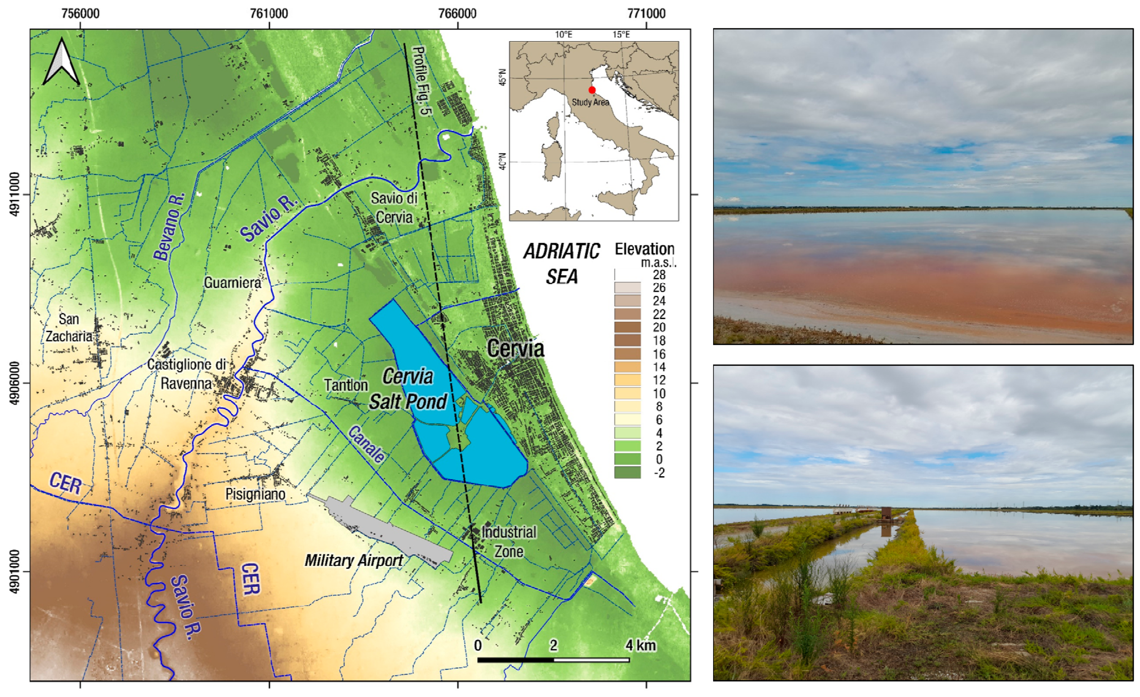
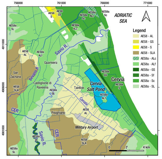
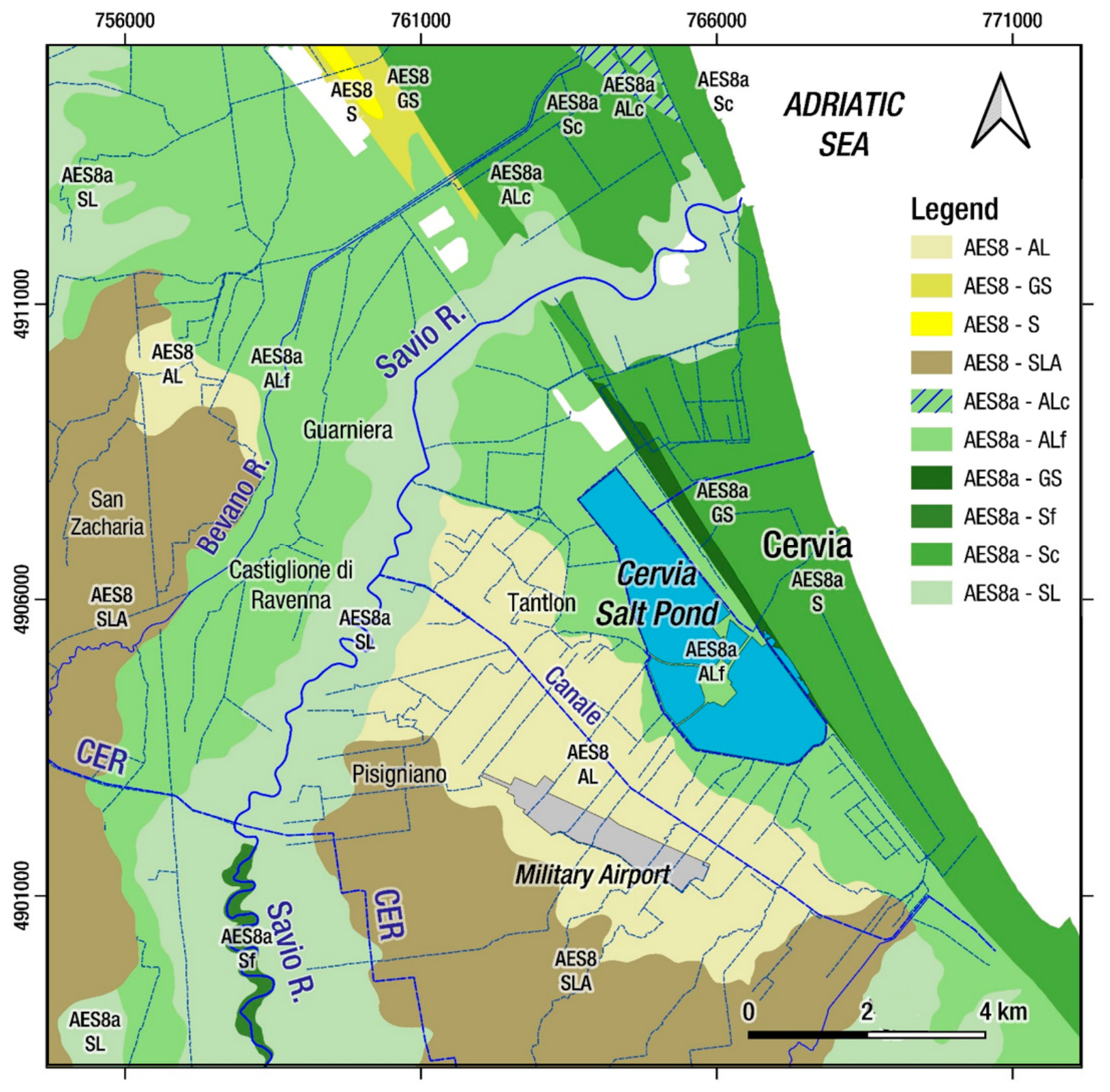
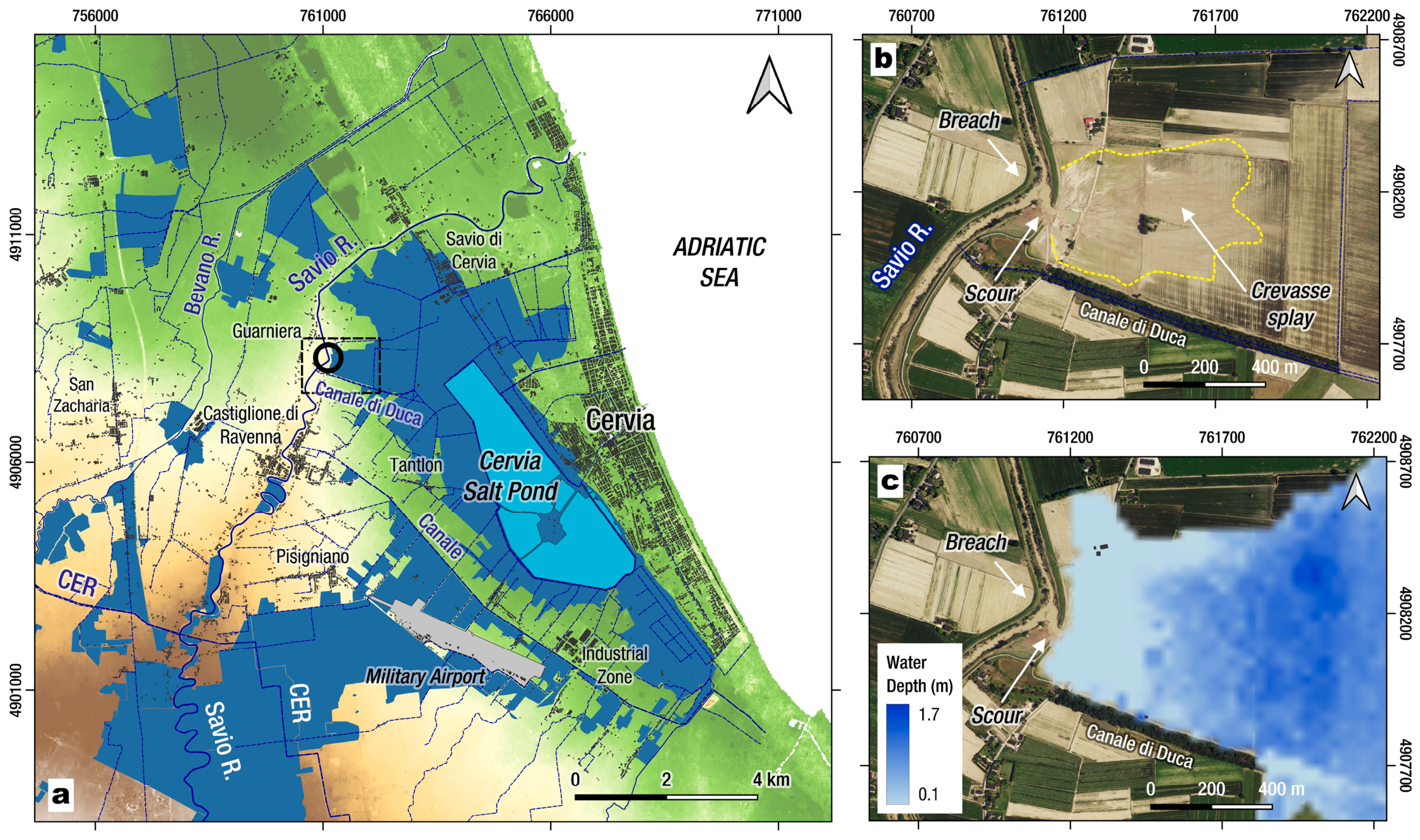
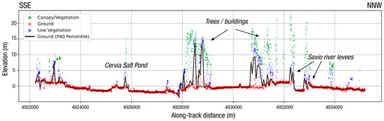
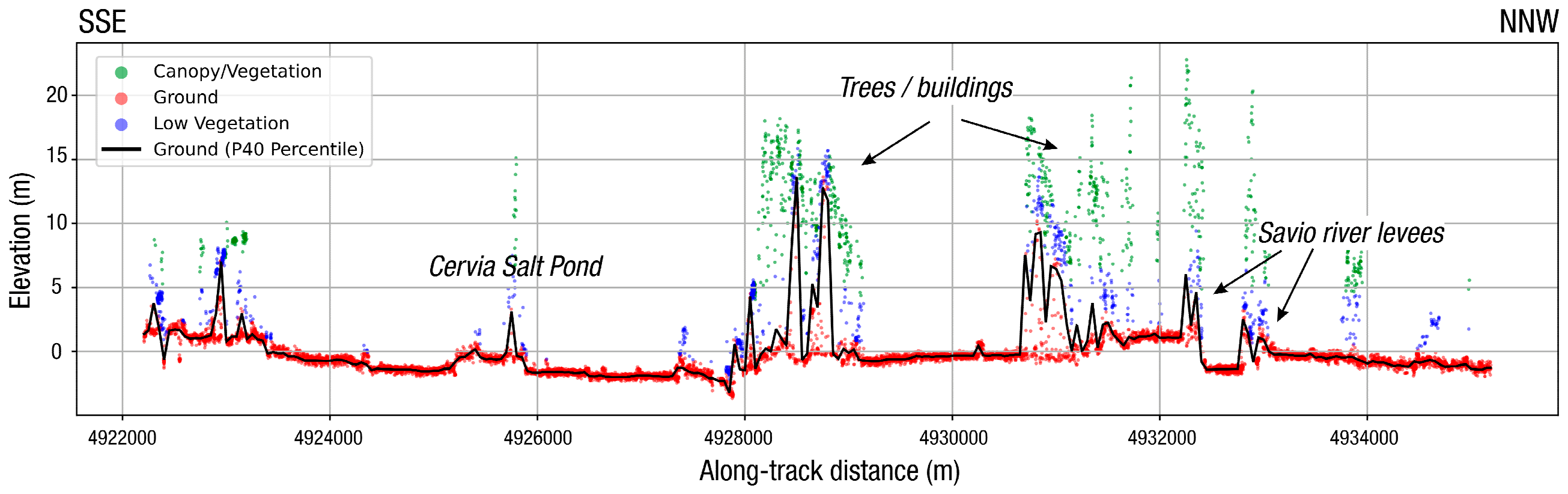
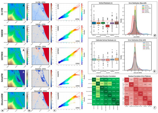
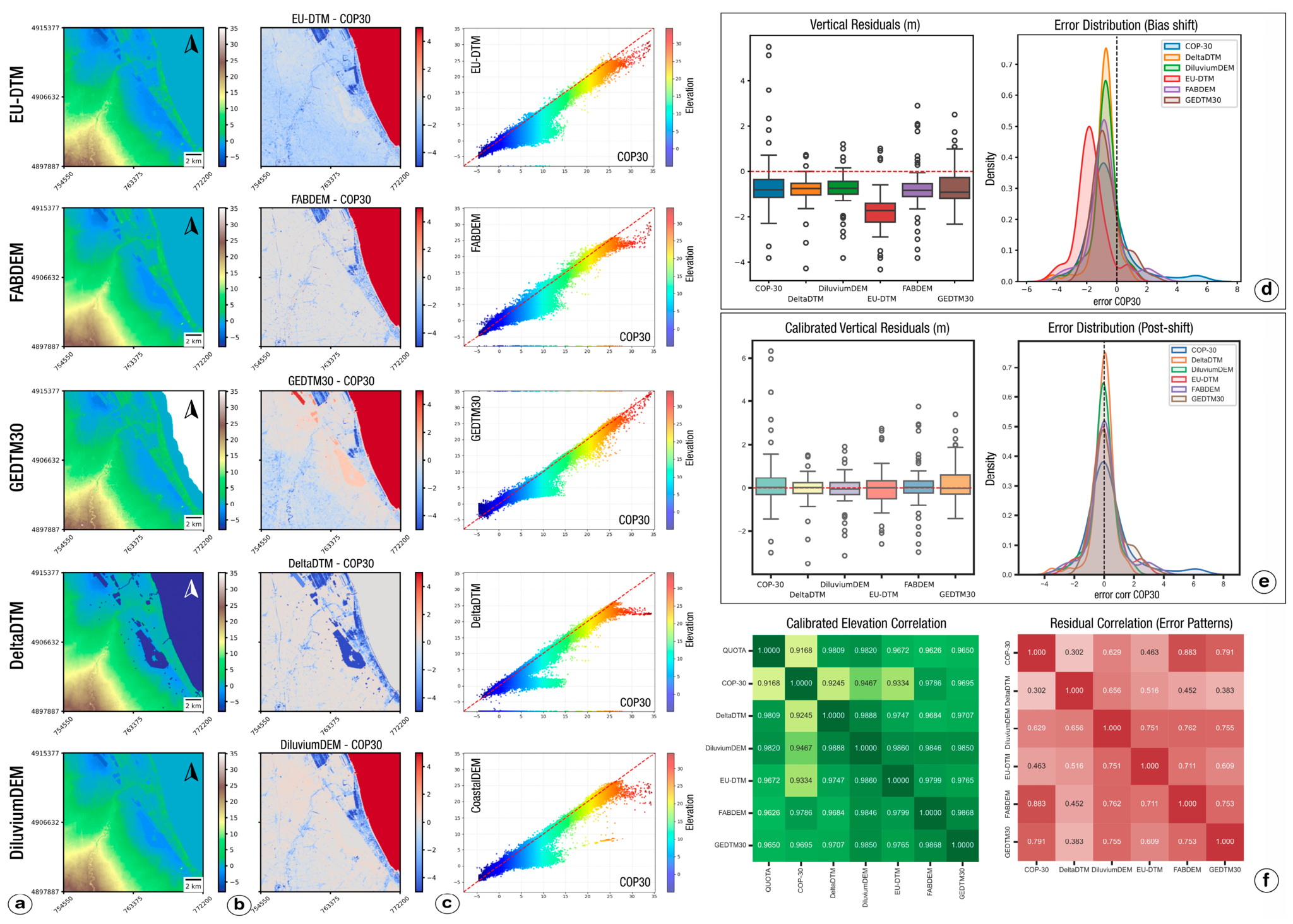
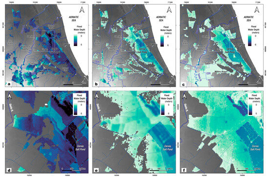
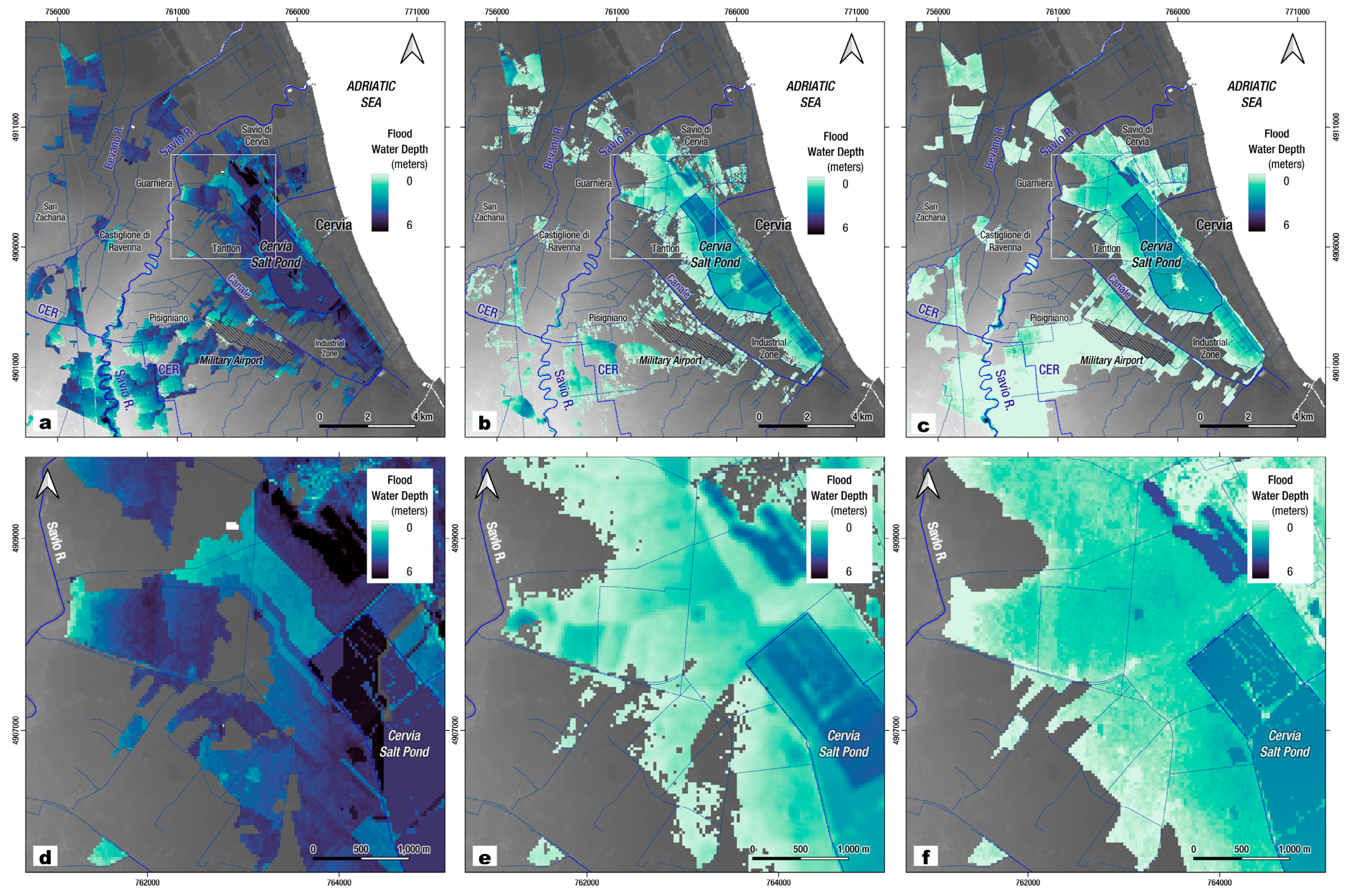
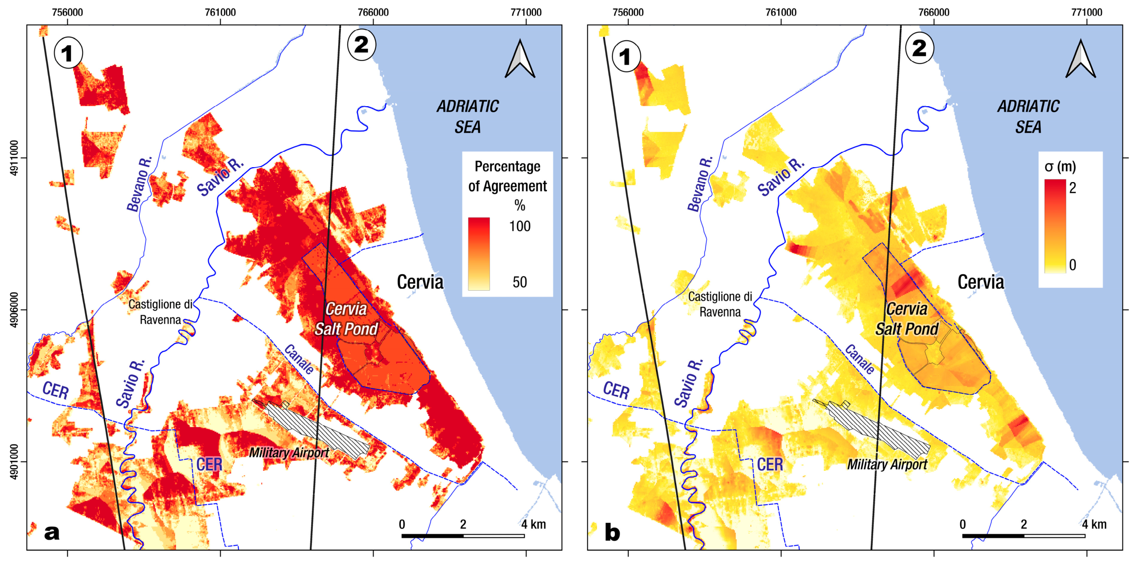
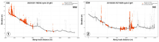
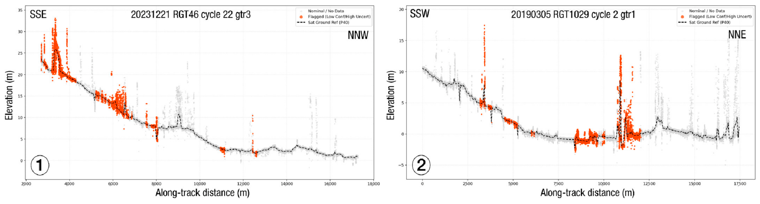
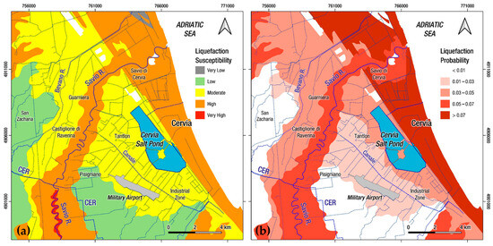
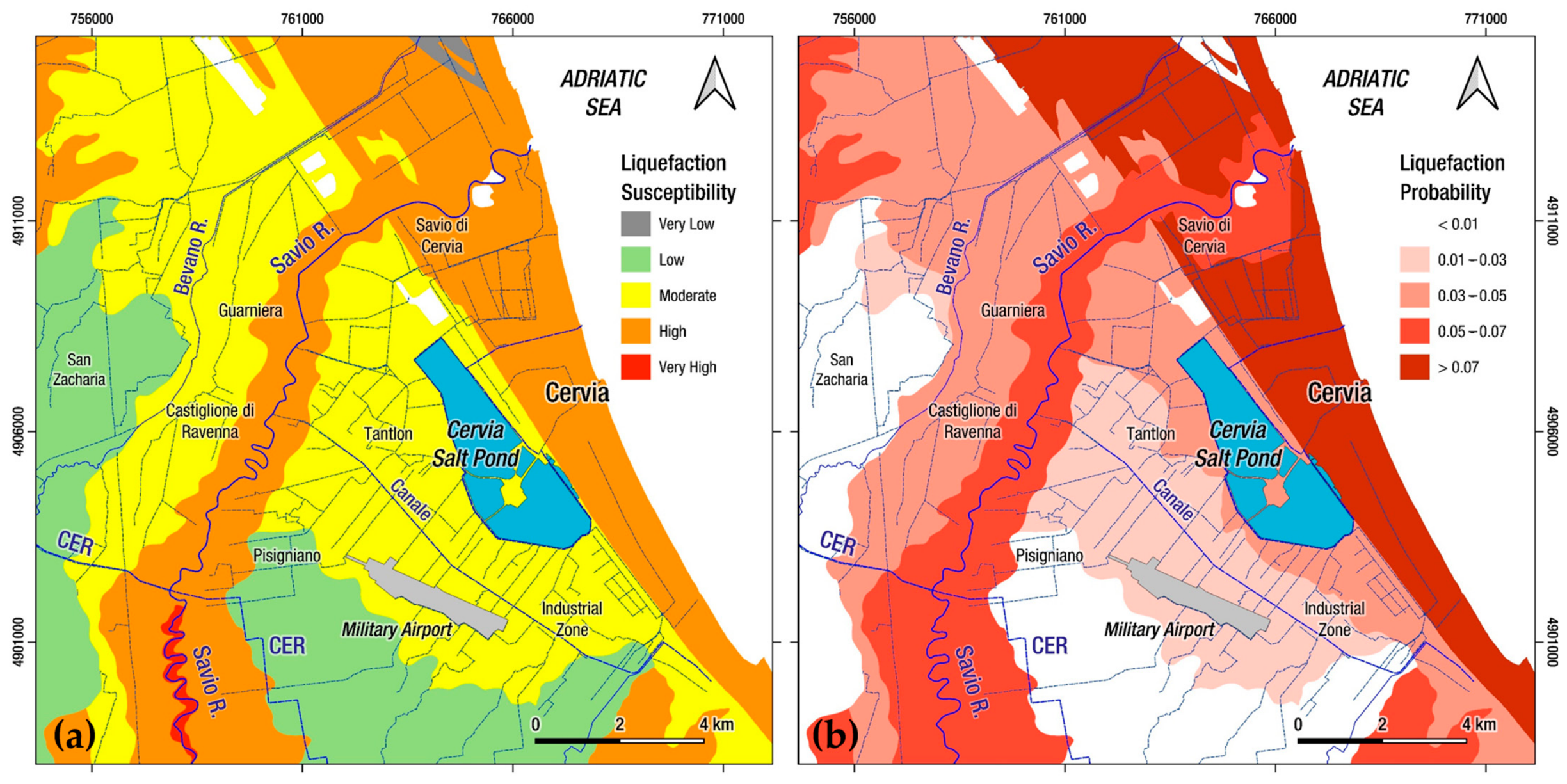
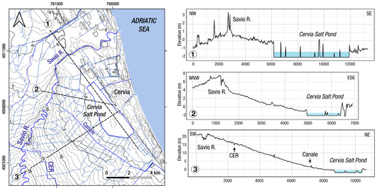
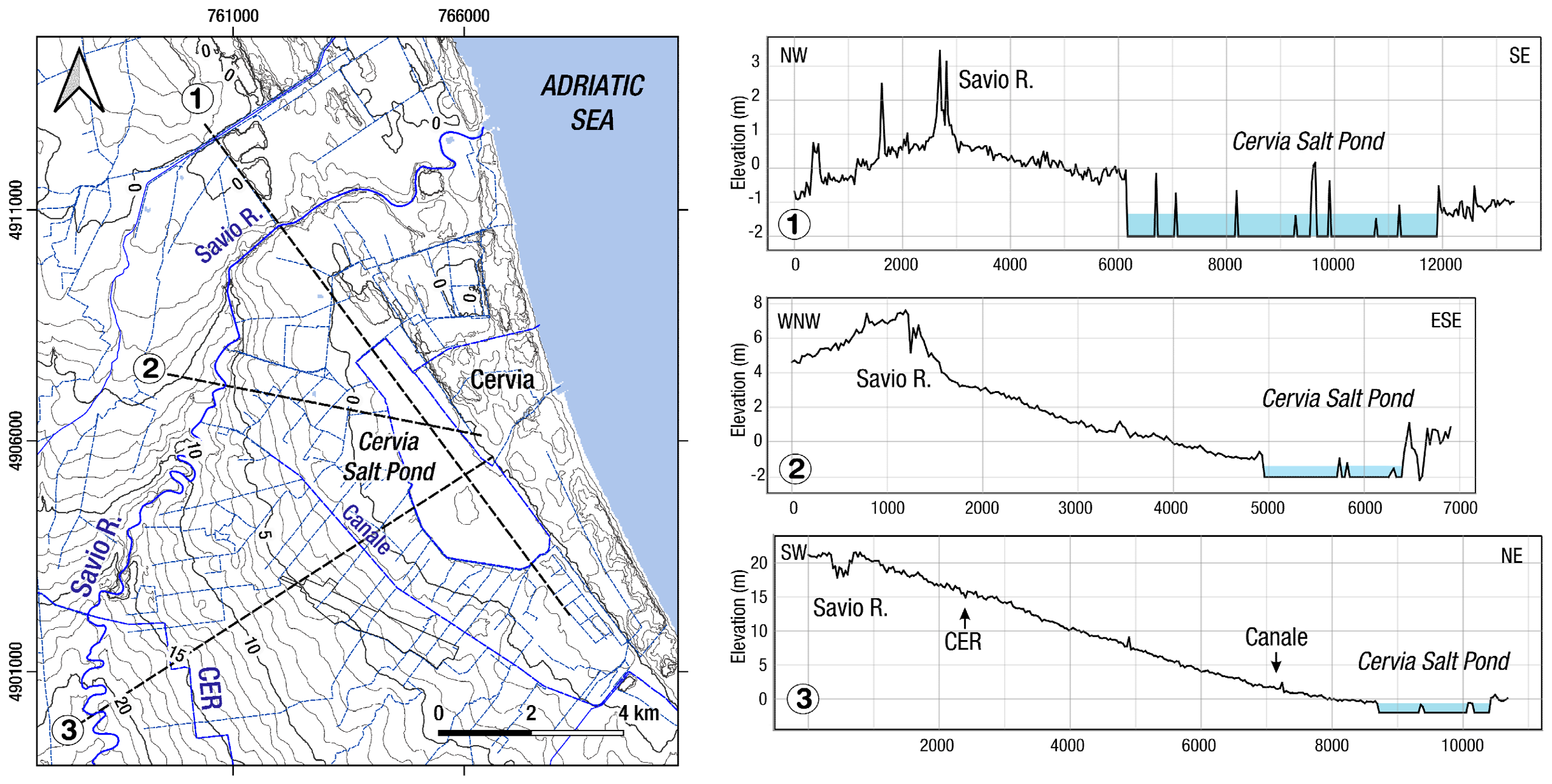
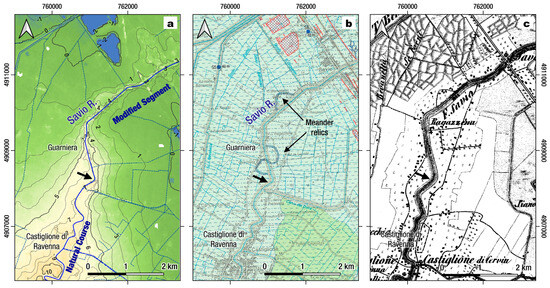
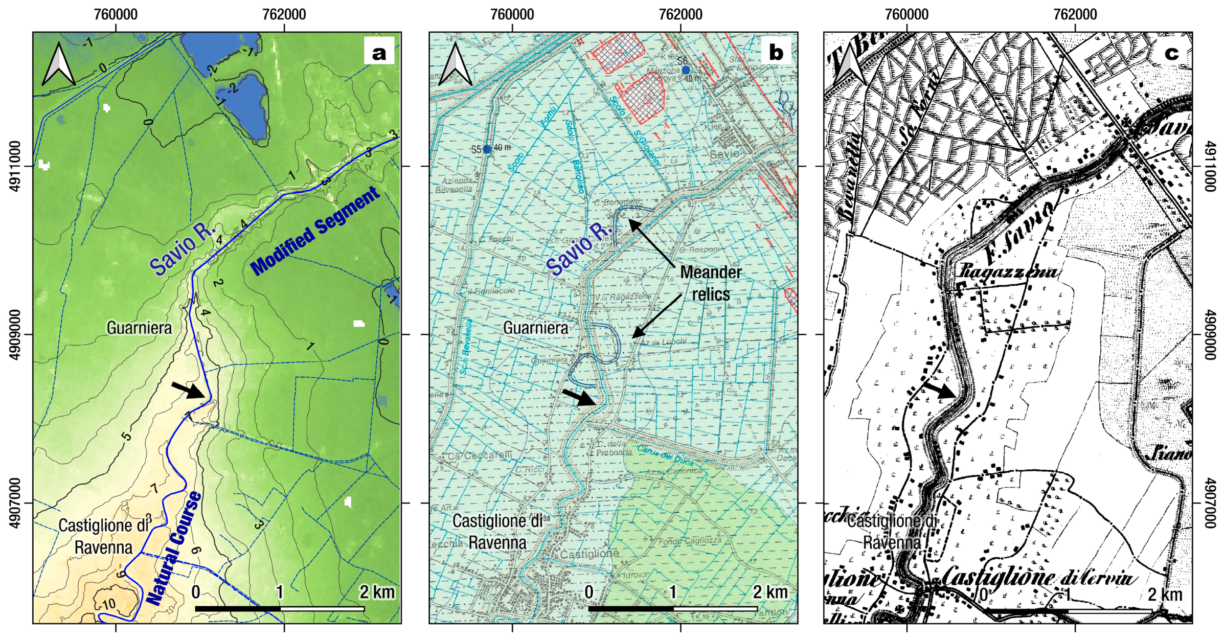
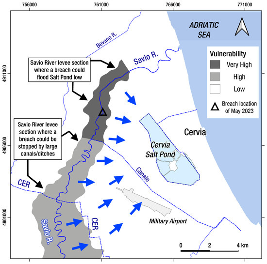
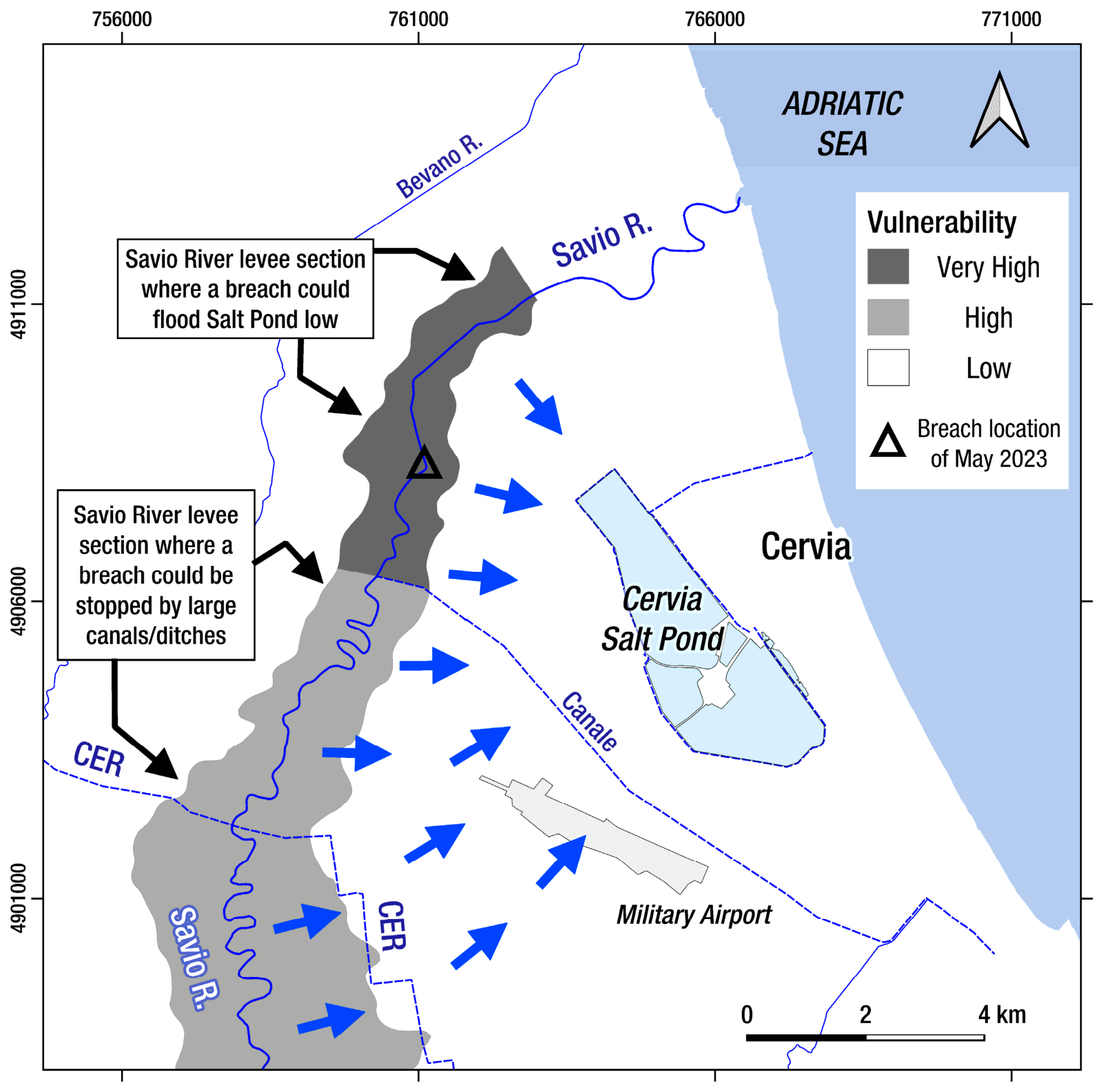

Disclaimer/Publisher’s Note: The statements, opinions and data contained in all publications are solely those of the individual author(s) and contributor(s) and not of MDPI and/or the editor(s). MDPI and/or the editor(s) disclaim responsibility for any injury to people or property resulting from any ideas, methods, instructions or products referred to in the content. |
© 2026 by the authors. Licensee MDPI, Basel, Switzerland. This article is an open access article distributed under the terms and conditions of the Creative Commons Attribution (CC BY) license.