


Abstract
This study uses and compares stationary and non-stationary Generalised Extreme Value Distribution (GEVD) to model the behaviour of nitrogen dioxide (NO2) emission maxima from each of 13 Eskom’s coal-fuelled power stations. The pollutant is modelled to facilitate monitoring and regulation in order to protect public health and the environment. The Maximum Likelihood Estimate (MLE) and Generalised Maximum Likelihood Estimate (GMLE) parameter estimation methods are used and compared in finding the best-fitting model per power station. The results show that a non-stationary model with time-dependent location and/or scale parameter(s) produced the best fit for ten of the power stations, while a stationary model gave the best fit for three, as confirmed by the diagnostic tools. Future extremely high NO2 emissions were estimated by making use of the 40 and 100 quarter return levels based on the best-fitting models. This study shows how stationarity may not hold for all NO2 emission data from Eskom’s coal-fired power stations. Modelling data using time-dependent non-stationary GEVD models can be useful, especially in identifying and predicting trends or patterns in worsening high NO2 emissions with time. This modelling approach is important in providing information for planning and policy formulation of extreme emissions from coal-fired electricity-generating power stations at Eskom (South Africa).
1. Introduction
In South Africa, coal-fired power stations are the main source of electrical energy, thus making them the major emitters of criteria pollutants [1]. Eskom, the power utility company in South Africa, owns and operates about 90% of these coal-fired power stations [1]. Of the 13 coal-fired power stations owned by Eskom, 11 are located in a single province, Mpumalanga [2]. This area is characterised by an abundance of coal reserves and is highlighted and ranked as one of the high-emission zones on the continent and the world [3]. The demand for electricity from Eskom is increasing as a result of urbanisation and population growth, which in turn increases the production of criteria pollutants in the atmosphere [4,5]. Nitrogen dioxide (NO2) is one such pollutant largely emitted during coal combustion in the generation of electricity [6].
Criteria pollutants produced from coal-fired power stations can pose a threat to human health [7,8,9,10,11] and the environment [12]. This is especially true in residential areas with a large population and/or in areas with close proximity to power stations [2]. Criteria pollutants are air pollutants for which National Ambient Air Quality Standards (NAAQS) are set to protect the environment and human health. There are set concentration limits, or criteria, for these pollutants in outdoor air.
Air pollutants may pose a threat, even when they are below regulatory limits [13]. The hypothesised emissions amounts required to prevent global temperatures from increasing beyond 2 °C above pre-industrial levels are expected to be exceeded in the near future [14]. This is likely to be realised when considering the total annual amount a country can reduce its carbon emissions [14]. Consequently, it can be deduced that pollutant emissions can be linked to deterioration of health or even death, especially at elevated (increased) concentrations.
The statistical modelling of emissions in general, and NO2 emissions from Eskom’s power stations in particular, may assist in understanding smog or explaining and predicting its behaviour in South Africa. Therefore, the accurate prediction of pollution episodes, including the size and length of the emission period, is crucial [15]. Parent statistical distributions concentrate their fit and explanation of emissions around where the bulk of the data is located. Although modelling the mean concentration of this pollutant using parent distributions is crucial, it is also important to understand the statistical behaviour of extremely high and rare concentration emissions that are largely ignored when using the parent distributions [16]. This is due to the exacerbated impact that could be caused by human activities and the environment’s exposure to these extreme emissions over a short time interval, if and when they occur. Extreme value models may thus provide a framework to facilitate the prediction of extreme pollution concentrations and to better understand their behaviour [15], especially in the case of Eskom in South Africa. Eskom is one of the biggest emitters in the world [17,18,19]. For example, in 2019, Eskom was the biggest emitter of SO2, exceeding the total emissions of the electricity sector of any nation globally, with the exception of India [20].
The current study then seeks to close this gap by fitting and comparing Extreme Value Theory (EVT) models to NO2 emissions from 13 of Eskom’s coal-fired power stations. The findings will provide a tool for predicting and explaining the risk associated with these extreme NO2 emissions.
The study of extreme emissions can be attained by considering the EVT distributions, namely: the Generalised Extreme Value Distribution (GEVD) and the Generalised Pareto distribution (GPD) as examples of the main extreme distributions. These distributions offer a robust, flexible method in their modelling and analysis, and are a valuable tool for estimating the magnitude and probability of these extreme events [21]. Both distributions have their stationary and non-stationary versions [21]. The GEVD approach possesses the flexibility of accommodating varied-tailed time series data by combining a family of three distributions into one distribution. The GEVD combines the extremal Weibull (short-tailed), Gumbel (light-tailed) and the Fréchet (heavy/fat-tailed) types into one distribution [22,23]. The Block Maxima approach is used to select extreme observations to fit to the GEVD.
Another flexibility of the GEVD is the modelling of observations such that observed maximums become or are independent and identically distributed, unlike the GPD, which can suffer from correlation of extreme observations as a result of the way the extremes are selected using the Peaks over Threshold (PoT) method [24]. The GEVD is also preferred for its simplicity over the GPD when fitting the observations to extremes. This is due to the subjectivity associated with the threshold selection process when fitting the GPD, which can be a problem for other practitioners [25]. This is especially true in the case of multiple samples, where one has to determine a threshold for each of the samples [26].
It is common to address the issue of skewness by log-transforming the data, or by making use of any other transformations when the skewness is due to the presence of a few outliers or extremes [27]. However, when there are many outliers and the data transformation fails due to high correlations in the PoT approach associated with the GPD, the Block Maxima associated with the GEVD gives independent observations. This, thus, offers the better option for the fit (see Dhanoa et al. [27] and references therein).
This study, therefore, assesses how suitable the GEVD approach (stationary or non-stationary) is for modelling quarterly maximum NO2 emissions from Eskom coal-fired power plants, highlighting the significance of accurate characterisation of extreme emission observation patterns.
1.1. Statement of the Problem
Emissions data, including NO2 emissions, may display non-stationary behaviour, and in such cases, non-stationary models may adequately represent the data compared to stationary models [21,28,29,30]. For example, some of the power stations in the current paper may not all display a stationarity behaviour, see the Augmented Dickey–Fuller Test for stationarity and the Mann–Kendall Trend Test. This paper applies both stationary and non-stationary GEVD models in modelling extremes of NO2 emissions from Eskom’s coal-fired power stations.
1.2. Justification of the Study
The Climate Change Bill, signed into law in July 2024 in South Africa, aims to address climate change by setting caps for major emitters, like Eskom, and requiring cities to publish adaptation plans. South Africa still faces challenges in transitioning away from coal and reducing its emissions.
Management and monitoring of extreme NO2 emissions is crucial for South Africa’s power utility company, Eskom. The pollutant is modelled to provide information that may facilitate the monitoring and regulation of NO2 in order to protect public health and the environment. The presence of potential upward trend patterns in NO2 emissions from Eskom’s coal-fired power stations can be an indication that the emissions are increasing/worsening with time. Such influence or association, if present, may be captured and incorporated in the modelling of the data for a more accurate prediction of future emissions. The stationary and non-stationary GEVD models are thus a good choice for modelling this data and in explaining the evolving levels of NO2 emissions, whilst monitoring and managing the emissions.
1.3. Objectives of the Study
The aim of the study is to model and describe the extremes of NO2 emissions from each of Eskom’s 13 coal-fired power stations using stationary and non-stationary GEVD models. This will be achieved by satisfying the following objectives:
- Fitting and comparing the stationary and non-stationary GEVD models to the Block Maxima NO2 emission data of each of Eskom’s 13 coal-fired power stations to find the best-fitting model.
- Comparing two parameter estimation methods, namely: Maximum Likelihood Estimation (MLE) and Generalised Maximum Likelihood Estimation (GMLE), in finding the best method to fit the GEVD models to describe each of the 13 coal-fired power plants’ NO2 emissions.
- Estimate the tail-related risk associated with NO2 emissions using return levels (of 40- and 100-quarters) for the best-fitting distribution of each power plant.
1.4. Significance and Contribution of the Study
To the best of our knowledge, there are no studies that model, describe and compare both stationary and non-stationary GEVD models on extreme NO2 emissions from coal-fired power stations in South Africa or in Southern Africa. The non-stationary model can incorporate covariates that capture patterns (trends, time, seasonality, etc.) that can be real or perceived [31]. The patterns can be captured in the parameters without altering the unit scale of the response or variable being modelled. This is beneficial for the interpretation of the results of the model. Whether real (physical in nature) or perceived (statistical), the influence of a covariate on the distribution of a variable can help in the prediction and understanding of extreme NO2 emissions from Eskom’s coal-fired power station for monitoring, regulation and future planning.
2. The Literature
The application of EVT models is not new to atmospheric emissions; from earlier studies, it is shown that extreme value methods were used in the monitoring of environmental data and modelling of trends thereof.
The GEVD was compared with 5 other EVT distributions, namely, the 2-parameter Gumbel, the 2- and 3-parameter GPD and the 2- and 3-parameter Weibull in the modelling of daily PM10 (particulate matter having an aerodynamic diameter of 10 micrometres or less) maximum concentrations in 3 monitoring stations in Malaysia, namely, Pasir Gudang, Bukit Rambai and Nilai. The data used was recorded for the period 2010–2012. The study made use of the MLE method and the method of moments parameter estimation. To assess the goodness of fit of the distributions, six performance indicators or accuracy measures (coefficient of determination, predictive accuracy, Index of Agreement and error measures that include the Normalised Absolute Error, Root Mean Square Error and Mean Absolute Error) were used. The GEVD gave the best fit in modelling the daily PM10 maximum concentrations across the three monitoring stations. Furthermore, the authors concluded that future extreme PM10 concentrations may be predicted using the GEVD [32].
In the modelling of hourly average air pollutants, namely, SO2 and NO2, from two monitoring sites (Alibeykoy and Umraniye) in Istanbul, Ercelebi and Toros [33] used the GEVD. The Gumbel’s Type I and Type II extreme value distributions gave a good fit for both pollutants. In their study, de Souza et al. [34] made use of various distributions to model monthly tropospheric ozone column O3 in the Central West region of Brazil for the period 2005–2020. The Kolmogorov–Smirnov, Anderson–Darling, Akaike Information Criterion, Bayesian Information Criterion, coefficient of determination and root mean square error tests were used to evaluate the model adequacy of the three distributions. For most months, the GEVD gave the best fit for the O3 data and with satisfactory performance measures.
Garbatov et al. [35] applied the extremal Weibull distribution to investigate the dispersion of extreme pollution and higher concentration probabilities of oxides of nitrogen (NOX) generated by ships while queuing in the winter seaport of Varna. They concluded that their developed and proposed method can be used in the analysis of air pollution concentrations and is a good representation when working with limited input information to obtain a satisfactory solution.
A study by Kütchenhoff and Thamerus [36] in Munich also made use of the GEVD, together with the GPD, to model daily air pollution data of NO2 and O3. The probability-weighted moments method was used for parameter estimation. For the monthly maxima of the NO2 and O3 concentrations, the GEVD gave a good fit.
Gouldsbrough et al. [21] developed a temperature-dependent extreme value model to characterise the magnitude and frequency of extreme O3 events and to determine probabilities for O3 exceeding health thresholds, as defined in the UK’s air quality index. The tails of the daily maximum O3 distribution were well described by the model at all 119 monitoring sites.
Hazarika et al. [29] used the GEVD to model concentrations of daily maximum O3 from Delhi, India, for the period 1 January 2011 to 31 December 2015. The presence of a trend, its significance, and seasonality in the time series were determined by the Sen’s method, the Mann–Kendall test and the Fourier transform technique, respectively. They used the Aikaike Information Criterion (AIC), Negative Log Likelihood, Bayesian Information Criterion (BIC) and the Likelihood Ratio (LR) test to determine the most suitable model for the daily maximum O3 data. The NOx, volatile organic compounds (VOCs) and meteorological variables were considered, individually and collectively, as covariates in the nonstationary GEVD models. The results showed that, for the stationary models, the median daily O3 maxima over Delhi were overestimated and the inclusion of covariates in the models showed improvement in fit. The GEVD with the extreme value index that is the heavy-tailed Frechet distribution was shown to be the best-fitting distribution under both stationary and non-stationary conditions for modelling daily maximum O3 concentrations from Delhi, India. A similar study was conducted where both the stationary and nonstationary GEVD gave a good fit in the modelling of extreme O3 in the period between 2000 and 2016, from 24 air monitoring stations in Peninsular Malaysia. This study used the probability plotting method based on goodness-of-fit statistics to assess how well the models performed [37].
Many other similar recent studies have modelled the extremes of air pollutants from different sources by making use of the GEVD and/or GPD models, or even their variants. Some of these studies make use of copulas, mixture or composite models, together with other techniques by employing more than one parent and/or EVT distributions to jointly model both the bulk and tails of air pollutants data, see for example [28,38,39,40,41,42,43,44,45,46,47,48,49]. The current paper, however, focuses on the extremes only and will thus be limited to the GEVD approach under stationarity and non-stationarity.
The choice of a covariate in the parameter of a non-stationary model is very important in physical events, such as those from a hydrological perspective. Matalas indicated the importance of differentiating and selecting between real, which is physical in nature, or perceived, which can be explained, say statistically, and not as a physical event [31]. Factors such as human influence, i.e., increased electricity demand due to growing population, urbanisation, industrialisation, etc., can lead to non-stationarity (trends) of emission data [4]. In a study such as the one by Sigauke and Bere [50], it was shown that natural factors such as temperature can contribute to the seasonality (and thus non-stationarity) of time series data. Their study was performed using the South African daily peak electricity demand for the period from 2000 to 2010. Additionally, it is indicated in Shikwambana et al. [4] that the winter season in South Africa (June, July and August) produced the highest mean concentrations of SO2 and NO2 in the Emalahleni and Middleburg regions, respectively, in the Mpumalanga province, South Africa.
Understanding and prediction of (long-term) extreme electricity demand is crucial [50]. Consequently, it is also important to understand extreme pollutant emissions because of the effects on human health and the environment [51]. Taking into account the requirement to meet the increasing demand for electricity, now characterised by load shedding in recent years [51,52], new power stations are required [6]. Coal is a readily available and cheap resource in South Africa. Understanding the combustion efficiency of coal-fired power stations is important in deciding whether to build coal-based power stations, as suggested by Lloyd [14] and/or non-coal-based power stations, as suggested by Marais et al. [6], in the near future to meet the electricity demand. It is for these reasons that the current paper seeks to model extreme NO2 emissions from Eskom’s coal-fired power stations in order to provide relevant information.
Historically, it is known that emissions intensify with time. Consequently, time will be used as a covariate in this paper. A proper highlight of the advantages and disadvantages of including a covariate in a non-stationary model compared to using a stationary model is given in Ragno et al. [53].
3. Methodology
This section discusses the various models used to analyse the data set on NO2 emissions at Eskom in South Africa, including stationarity tests, the GEVD Extreme Value Theory (EVT) model, parameter estimation and model selection and diagnostics.
3.1. Test for Stationarity and Trend Detection
To test the potential non-stationarity in the quarterly block maxima of NO2 emission data, the Augmented Dickey–Fuller (ADF) test will be used as a preliminary diagnostic tool. It is used for data exploratory purposes only, and not for confirmatory purposes.
To test for monotonic trends in the NO2 emission data blocks, the non-parametric Mann–Kendall (MK) test is performed [54]. This test does not assume the normality of the data. The null hypothesis is given as:
H0.
There exists no trend in the extreme NO2 time series.
H1.
There exists a trend in the extreme NO2 time series.
3.2. Modelling Maxima Random Variables (GEVD)
In EVT, the Block Maxima (BM) technique divides the observation period into equal, non-overlapping intervals (blocks). It focuses just on the maximum values found inside each block. This approach helps to estimate the tail behaviour of the distribution, i.e., the extremes [22,55].
Let denote a set of maxima chosen from each of the m blocks inside the dataset. The selection of block size for the block maximum method is contingent upon factors like instrument constraints, seasonal trends, and the intended objective of the analysis, leading to varied block sizes from hourly to annual intervals.
In this study, quarterly blocks from datasets of 60 to 108 monthly NO2 emissions observations are used, and this choice is motivated by statistical and physical considerations. NO2 emissions can show seasonality patterns [4] and as such, a three-month block corresponds with seasonal dynamics, allowing the assessments of extremes within generally consistent conditions of the atmosphere while moving away from the mixing of unique seasonal processes. From a statistical point of view, quarterly blocks provide a tradeoff between sample size and block length. For example, monthly blocks would be too short to sufficiently represent the behaviour of extremes, while annual blocks would give a sample size of 5 to 9 observations, which would be too small for extreme value analysis. On the other hand, quarterly blocks give a sample of 20 to 36 observations, allowing for a more stable estimation.
The maximums, s, are subsequently modelled using the Generalised Extreme Value Distribution (GEVD).
3.2.1. Stationary Data Models
A GEVD is regarded as a stationary model if its parameters are constant over time, with the assumption that they will remain constant over the fitted data timeline [30,56]. In stationary data models, the GEVD is fitted to Block Maxima with a cumulative distribution function (CDF) given as
where the location, scale and shape parameters are represented by and , respectively. determines the GEVD shape type and thus tail heaviness of the data, as follows [22,23,57]:
- If , then belongs to the light-tailed Gumbel-type distribution (Type 1).
- If , then belongs to the heavy-tailed Fréchet-type distribution (Type 2).
- If , then belongs to the short-tailed extremal Weibull distribution (Type 3). This distribution is bounded above by [58].
3.2.2. Non-Stationary Data Models
In a non-stationary model, the parameters of the probability distribution change as a function of time or in response to changes in a certain covariate [59]. In Coles [30], it is indicated that if the mean and variance of emissions increase with time, a logarithmic data transformation will tame the variance and differencing the data returns (taking a log of ratios of successive observations) will get rid of the trend, thus the data will then approximate stationarity. Also indicated in the text as an option is the fitting of a non-stationary EVT distribution using the GEVD by incorporating a covariate, such as time, in the parameters of the stationary model. The CDF can be obtained by including a time covariate and thus adapting Equation (1) above. In this paper, four non-stationary models will be considered in addition to the stationary model represented by Equation (1) or Model 0. A summary of all these models is presented in Table 1 below.
Table 1.
Model representation and parameter transformation(s) under the non-stationary GEVD and effect on NO2 emissions quantification.
Where and can be time-dependent parameters to be estimated under the non-stationarity assumption, with time coefficients given by and for the location and scale parameters, respectively, and and are baseline constant parameters for the time-dependent parameters. is the constant shape parameter applicable to both the stationary and non-stationary models. can be negative to signify emission improvement or reduction efforts at the power station using the latest abatement technology. Similarly, can be negative to signify variation reduction efforts at the power station using the latest technology.
The general expression for the non-stationary GEVD is given as [30],
Taking Model IV, for example, according to Maposa et al. [60], the CDF is then presented as:
3.3. Parameter Estimation
Many parameter estimation methods exist for stationary and non-stationary methods. They include, but are not limited to, Maximum Likelihood Estimation (MLE) [30,61], L-moments [62], probability-weighted moments [63] and the Generalised Maximum Likelihood Estimation (GMLE) [64]. Since the MLE method does not always produce reliable shape parameter estimates (when ) [65], the inclusion of the GMLE can also be considered. Xavier et al. [56] stated that the GMLE possesses the flexibility of being easily adaptable to the probabilistic framework changes in the series, facilitating the adoption of non-stationary GEVD models. However, the MLE can also perform well over other techniques due to its flexibility and adaptability to changes in model structure [30]. This includes parameter estimation with time-dependent time parameters [66], especially for sufficiently large samples [64].
Two methods of parameter estimation will be used in this paper, the MLE and the GMLE. They will be compared in the analysis of stationary and non-stationary models. For illustrative purposes, the MLE and GMLE methods will be shown for non-stationary GEVD models only. The stationary version can be obtained by substituting the time-dependent parameters, and with the stationary GEVD parameters, and , respectively.
Let be quarterly NO2 maxima following a GEVD, where is the number of quarters.
3.4. Maximum Likelihood Estimation (MLE)
If , the likelihood function for the distribution in Equation (2) is given by Coles [30] and Maposa et al. [60] as:
Then the log-likelihood is given as follows:
Generalised Maximum Likelihood Estimation (GMLE)
The Generalised likelihood function for Equation (2) if is given by
where
- is the likelihood function in Equation (4),
- is the prior distribution for the shape parameter, and is the Beta distribution.
The GMLE is an extension of the MLE method [67] and a special case of the Bayesian method [64] where the prior distribution is based only on the shape parameter, . is the default prior in the GMLE method of the GEVD parameters [64,68]. It incorporates the prior into the likelihood function of the MLE method by taking the product of and to obtain the in Equation (6). A significant benefit of employing the GMLE approach is the capability of incorporating additional information, including historical and regional information, to define the prior distributions [64,69]. In small samples, the MLE may give unreliable values of the shape parameter, . Additionally, the likelihood equations can be complex and analytically unsolvable [67]. In such cases, the GMLE method is a preferred alternative [69].
Maximising the log-likelihood in Equation (7) below, the GMLE estimator can be obtained [64,67,69].
Taking the partial derivative with respect to each of the parameters of the log-likelihood in Equations (5) and (7) and equating them to zero, the parameter estimators can be obtained. In the log-likelihood in these equations, the shape parameter () was kept constant.
A detailed explanation of the GMLE estimator for the stationary and nonstationary GEVD can be found in Martins and Stedinger [69], Araveeporn and Sukpan [67], El Adlouni et al. [64] and Xavier et al. [56].
The MLE and GMLE estimators for the GEVD where can be similarly obtained.
3.5. Model Selection
The Likelihood Ratio (LR) test will be used to test whether the incorporation of time in the parameters of a non-stationary model improves the stationary model or not. A p-value of less than the significance level implies that the addition of time in the parameter(s) is statistically significant [68].
Additionally, the Akaike Information Criterion (AIC) [70] values will be used to compare all the models at a power station. A model with the lowest AIC value will be considered to be the best fit for the power station data. The AIC equation is given as:
See, among others, Min and Halim [71], De Leo et al. [65] and Prahadchai et al. [66].
3.6. Model Diagnostic
To assess the goodness of fit of the GEVD models (both stationary and non-stationary), the diagnostic plots (namely Probability (PP), Quantile-Quantile (QQ) and Density plots) are among other tools used. The PP and QQ plots are used to check if the percentiles and quantiles, respectively, of the data and their fitted theoretical distributions come from the same underlying distribution [72]. In the non-stationary case, it is of note, as indicated by Gilleland and Katz [68] that, “the first quantile-quantile and density plots are on the Gumbel transformed scale (the data are transformed to a stationary sample)”. In addition to the diagnostic plots, the model adequacy of the stationary GEVD models will be assessed using the Kolmogorov–Smirnov goodness-of-fit test.
3.7. Return Level Estimation
The return level is the value/level of NO2 emissions expected to be exceeded with a certain probability, say 5% chance per year.
Let be the occurrence probability of an extreme event defined as the change of the event occurring at least once, on average, in years [71]. In simple terms, is the level that is expected to be exceeded on average once in T years [30]. Equating the cumulative distribution to and solving for we get the return level as follows.
For the stationary GEVD model
For the non-stationary GEVD models
4. Results
4.1. Description of Data
In this study, the dataset consists of monthly NO2 emissions per station, obtained from Eskom, spanning a period of 60 to 108 months, covering the years from 2005 to 2014. The monthly observations from each of the 13 power stations were grouped into quarters of a year called blocks. Thus, blocks consists of three months each such that there are 20 to 36 blocks per power station.
The data is presented in the Supplementary Materials and include the variables, power station itself, Nitrogen dioxide (NO2) given in tons, and date of emission.
4.2. Descriptive Statistics
Figure 1 below shows the time series plots for the monthly Block Maxima of NO2 emission in tons. Random spikes can be observed from the two power stations, suggesting the presence of extremes in the data. For the Lethabo power station as an example, an obvious decreasing trend in the mean NO2 emissions is observed with time, while for Matimba, an increasing variance is suggested with time. The choice of the BM approach in modelling this data is beneficial to cater for any dependence in the data [24].
Figure 1.
Time series plot of NO2 emissions quarterly maximums (in tons) for all of Eskom’s power stations.
4.3. Testing for Stationarity and Monotonic Trends
Table 2 presents the Mann–Kendall trend test results for the BM data of the 13 power stations. Most of the power stations suggest non-stationarity of the BM data since the test has a p-value > 0.05 for the stations. The results for Duvha and Kriel power stations, with p-value < 0.05, suggest otherwise. However, these results are exploratory and not confirmatory in nature, since we are working with block maxima.
Table 2.
Augmented Dickey–Fuller Test for stationarity and Mann–Kendall Trend Test on BM data.
To verify these results, the Mann–Kendall trend test is used. The results indicate the presence of a statistically significant trend in the quarterly BM data for all power stations, with the exception of Arnot, Matimba, and Matla, at a 5% significance level, since the p-value for these three power stations exceeds 0.05. The power stations, Camden, Grootvlei, Komati, Majuba and Tutuka demonstrated a significant and increasing trend, while a significant but decreasing trend is observed for the Duvha, Hendrina, Kendal, Kriel and Lethabo power stations. These results are consistent with the time series plots in Figure 1.
To further explore the data, Figure 2 below shows the box plot for the BM data from each of Eskom’s power stations during the study period. The power station to emit the highest monthly maximum NO2 is Majuba followed by Lethabo and the lowest monthly maximum is Komati followed by Grootvlei.
Figure 2.
Box plot for the quarterly BM data for each of Eskom’s 13 coal-fired power stations. The lower and higher boundaries of the box reflect the first (Q1) and third (Q3) quartiles, respectively. The central line and the red dot within each box denote the median and mean, respectively. The whiskers extend to extreme observations within 1.5 times the interquartile range (IQR) of the quartiles, where IQR = Q3 − Q1. Data points outside the whiskers indicate potential outliers that exceed Q3 + 1.5 IQR or fall below Q1 − 1.5 IQR.
4.4. Generalised Extreme Value Distribution
The current section looks at model fitting, parameter estimation and model diagnosis of the GEVD.
4.4.1. GEVD Model Fitting (The LR-Test and Parameter Estimation)
Since the results of the MK test (and ADF test) above suggest non-stationarity of data for most stations, non-stationary models can be considered. Table 3 shows the LR test results of the four non-stationary GEVD against their corresponding stationary model for each of the 13 power stations.
Table 3.
The LR-test (Test statistic, p-value) and AIC for each of the models.
In Table 3 below, the LR-test results use the stationary GEVD, discussed earlier, as the basis of comparison against each of the non-stationary models. In simple terms, one wants to see if the incorporation of time in the parameters as a covariate improves the original stationary GEVD model or not. This is done for all non-stationary models (Models 1, 2, 3 and 4) per power station. A p-value < 0.05 indicates that the inclusion of time in quarters as a covariate in the parameter(s) of the non-stationary model improves the stationary GEVD model and is thus statistically significant. The model with the lowest AIC value (and usually the lowest p-value) is considered the best non-stationary GEVD for that power station.
From Table 3, ten of the power stations, namely, Camden, Duvha, Grootvlei, Kendal, Komati, Kriel, Lethabo, Majuba, Matimba and Tutuka, have at least one non-stationary GEVD model that shows improvement in model fit after incorporating time in either one or both parameters ( ). This is according to the LR test with p-values smaller than 0.05, and the AIC values that are the smallest for these power stations. It is worth noting that in this paper, a model obtained by using MLE parameters is only considered reliable if the shape parameter is bigger than −1 () [65].
For Camden, all of the MLE non-stationary models, Models 1, 2, 3 and 4, showed improvement in fit after incorporating time in either the location, , and/or scale ()/logscale (), while only one of the GMLE models, Model 2, showed an improved fit after incorporating time in the scale parameter. According to the AIC and p-values of the LR test, the best model for Camden is the MLE Model 1. However, since the MLE shape parameter for all non-stationary models under the MLE method is smaller than −1, Model 2 of the GMLE method is considered the best for the power station. Similarly, all of Komati’s non-stationary models under the MLE method, with LR test p-value < 0.05, have . As a result, Model 4 of the GMLE method, with the lowest AIC and LR test p-value, is chosen as the best model for the power station. In the case of Komati power station, it is of note that all but one (the GMLE Model 3) non-stationary models improved their associated stationary models. On the other hand, none of the non-stationary models for Arnot and Matla improved their associated stationary model since their LR test p-values were bigger than 0.05 and since their AIC values were bigger than those of the associated non-stationary models. In Table 3, Hendrina’s non-stationary models failed to significantly improve their associated stationary model, with big AIC values and LR test p-value 1. Additionally, both the MLE and GMLE stationary models for Hendrina also gave very big AIC values, indicating that none of the models for the power station gave a good model for the data. Similarly, all GMLE non-stationary models failed to significantly improve the stationary model for Majuba and Matla, with a big AIC value and LR test p-value of 1.
The rest of the power stations can be similarly interpreted. Table 4 below presents the summary of which distribution is the best for each of the power stations and why.
Table 4.
Summary and the reason for selecting the best model for the BM data of each power station.
4.4.2. Parameter Estimation
The current section explores the parameter estimates of the best-fitting GEVD. The shape parameter, the location and scale parameters are estimated.
Testing for the shape parameter
The GEVD model incorporates three distributions (extremal Weibull, Gumbel and the Fréchet). The extremal distribution with has a bounded tail; the Gumbel distribution with has a light tail and the Fréchet distribution with is heavy-tailed. These properties of will be used to classify the best model fit for the data of each power station. This is done by investigating the shape parameter estimate, , and the 95% confidence intervals (CIs). A CI that includes a zero suggests that the maxima data may follow the Gumbel distribution. Table 5 presents the shape parameter estimates, together with their 95% confidence intervals for each power station. The confidence intervals were obtained by the profile likelihood method [68]. Also included in the table are the AIC values for the GEVD and the Gumbel distribution for comparison purposes. Similarly to the previous section, a lower AIC value indicates a better model.
Table 5.
Shape parameter estimates for the fitted GEVD, and the LR-test for comparing the GEVD against the Gumbel distribution. Also given is the AIC of the two distributions.
In Table 5, the shape parameter point estimate is negative, for all 13 power stations. Since the confidence interval of the shape parameter () for five of the power stations, namely, Arnot, Kendal, Kriel, Majuba and Matla is negative and does not contain a zero, is significantly negative and different from zero. This means that the data can be modelled using the short-tailed extremal Weibull class distribution for these power stations. However, seven power stations, namely: Camden, Duvha, Grootvlei, Komati, Lethabo, Matimba and Tutuka have a confidence interval containing a zero, suggesting that the power stations have data that may follow a Gumbel class distribution (). To verify these results, the following hypothesis is tested by making use of the LR test as follows,
H2.
The data follows a Gumbel type 1 distribution ().
H3.
The data do not follow a Gumbel type 1 distribution ().
Of the seven power stations, the LR test in Table 5 produced a p-value greater than 0.05 for four stations, namely, Camden, Grootvlei, Matimba and Tutuka. This result suggests that we fail to reject the null hypothesis and conclude that the power stations’ data follow a Gumbel type 1 distribution. For Duvha, Komati and Lethabo, however, a p-value smaller than 0.05 was obtained, indicating that these power stations belong to the short-tailed extremal Weibull class distribution. The AIC values also confirm and agree with the results of the LR test for all but two power stations, Matimba and Tutuka. In other words, for these power stations, the lowest AIC values were obtained for the GEVD, despite the LR test p-values exceeding 0.05. However, an examination of the BIC values (not included here) shows consistency with the p-values from the LR test; the BIC values for the Gumbel distribution are smaller than those of the GEVD. As a result, one may conclude that Matimba and Tutuka follow a Gumbel distribution.
Regarding Hendrina power station, no reliable confidence interval could be obtained since the power station did not give a good fit for any GEVD model. However, based on the AIC values of the power station in Table 5, the Gumbel distribution (with AIC = 563.67) gave a good fit compared to all the GEVD models in Table 3 for the power station. Although the main purpose of comparing the GEVD with the Gumbel is the determination of whether is equal to zero or not, the Gumbel distribution performs relatively well in modelling the Hendrina power station data compared to all (stationary and nonstationary) GEVD models in this paper, and as such, will be considered the best model for the power station going forward.
The location and scale parameters
This section presents the location and shape parameters of the best-fitting model for each of the stations. Table 6 presents a summary of the parameter estimates of the overall best-fitting GEVD model across the two estimation methods for each power station. The last column shows the parameter equations where the non-stationary GEVD model is the best-fitting model for the power station.
Table 6.
Parameter estimates for the best-fitting model.
In Table 6, the model that gave the best fit for Arnot and Matla is the stationary GEVD with all parameters as constants since they do not have a non-stationary model that improved their associated stationary model, as indicated above.
From Table 6, the non-stationary GEVD model with time-dependent location parameter, Model I, produced the best fit for Grootvlei and Lethabo. Since for Grootvlei, more emissions are, on average, produced over time for the power station, while for Lethabo, fewer emissions are produced over time (with ). This is consistent with the time series plots in Figure 1. The variation from the power stations is constant over time, that is, and for Grootvlei and Lethabo, respectively.
The non-stationary GEVD model with time-dependent location and scale parameters, Model II, produced the best fit for Camden and Duvha. The power station in Camden has since , indicating an increase in NO2 emissions with time. However, for Duvha, a decrease in the mean of NO2 emissions in tons over time is observed since . The variation for both power stations decreases with time since for each station. This indicates that the power station is not as noisy over time. Installed abatement technologies may have an influence on these results.
The best fit for Matimba was produced by the non-stationary model with a time-dependent log scale parameter, Model III. The Matimba plant has more variation since is a constant and is positive for all .
Model IV, the non-stationary GEVD model with time-dependent location and log scale parameters, produced the best fit for Kendal, Komati, Kriel, Majuba and Tutuka. Of the five power stations, three, namely Komati, Majuba and Tutuka, have , indicating that the power stations have emissions that increase over time. The variation for all five power stations decreases with time since .
The rest of the power stations can be similarly interpreted, with all parameters summarised in Table 6.
4.4.3. Model Diagnostics
The diagnostic plots, namely, PP-plots, QQ-plots and Density plots for the best-fitting models are presented in Figure 3. For illustrative purposes, results for two power stations, namely, Lethabo and Matimba, are presented.
Figure 3.
PP-plots, QQ-plots and Density plots of the best-fitting GEVD for (a) Lethabo and (b) Matimba power stations, respectively.
In Figure 3, the PP and QQ plots for Lethabo and Matimba power stations have points that do not deviate much from the 45° line. This suggests that the selected GEVD model, that is, the non-stationary GEVD with , and the non-stationary GEVD with , does give a good fit for the maxima data of Lethabo and Matimba power stations, respectively, both under the ML estimation method. The density plots also show a good fit, as the empirical curve is not that far off from the theoretical curve for both power stations. It can thus be concluded that the GEVD, with its various forms, is a good fit for the data of the power stations. The other data of the other power stations can be similarly interpreted.
4.4.4. Return Level Estimates
In this section, we will have a look at the return periods and return level estimates of the best-fitting model for each power station, and these are presented in Table 7.
Table 7.
Return periods and return levels estimates based on the best-fitting model for each of the 13 power stations.
The return levels for power stations with a stationary model as the best-fitting model, namely, Arnot, Hendrina and Matla, are given in Table 7. This model represents a power station operating optimally. Thus, the return level estimate does not depend on time for this model. Using the Arnot power station as an example, the 40- and 100-quarter return levels are 5050.04 and 5101.09 tons, respectively. This means that 5050.04 tons of NO2 emissions are expected to be exceeded at least once in 40 quarters, and 5101.09 tons of emissions at least once in 100 quarters. The 100-quarter return level exceeds the maximum value of the current data, given in Figure 2, but the 40-quarter return level does not. This means that the maximum value of the current data is expected to be exceeded at least once in 100 quarters. For Hendrina, the maximum NO2 of 5723.00 tons is exceeded by both the estimated 40 and 100 quarter return levels. However, both of the return level estimates did not exceed the maximum value of 11,512.92 for the Matla power station.
In their study, Vanem [73] indicates that, for non-stationary models, return levels and return periods ought to be treated differently compared to the traditional stationary case. However, one can treat return levels as a function of the covariate, in our case, time in quarters, by finding corresponding quantiles of the distribution, which would then be a function of the time. In Table 7, quantiles that correspond to the 40- and 100-quarter return levels are calculated for the first and last quarters of the datasets for each power station. For Grootvlei, as an example, we have Q1 and Q20, representing quarter 1 and quarter 20, which are the first and last data points of the maxima time series dataset, respectively.
One can see that the return level estimates in Table 7 are indeed different between the first time point Q = 1 and the last time point (Q = 20 or 36) for each of the power stations where a nonstationary model is the best model for the power station. This indicates the effect of incorporating time in the location and/or scale parameter on the return levels. As a result, it is of importance to check if the difference (Q20 − Q1) is statistically significant or not. This will be achieved by considering the 95% Confidence Intervals (CI) of the difference. A CI that does not contain a zero indicates that the difference is statistically significant, and one that contains a zero indicates that the difference is not statistically significant. These CIs are based on a normal approximation [68]. Additionally, a difference with a negative sign indicates a decrease in tons of the estimated return level from the first to the last quarter of the dataset, and a positive sign represents an increase.
Taking the Matimba power station as an example, it can be observed from Table 7 that the 40- and 100-quarter effective return level estimates from quarter 1 to quarter 36 increased by a value of 959.87 and 1077.05 tons, respectively. That is, a return level difference of 959.87 and 1077.05 tons, with a 95% CI of (354.00; 1565.74) and (385.89; 1768.22) for the 40- and 100-quarter effective return. Therefore, for Matimba, the increases are statistically significant since the confidence interval does not contain a zero. This is an increase of 15.35% and 17.12% for the 40 and 100 quarter return levels, respectively, from the first quarter to the last quarter. On the other hand, for Kriel power station, the 40 and 100 quarter return level difference of −4114.018 with 95% CI of (−7455.067; −772.9698) and −4734.763 with a 95% CI of (−8726.58; −742.9453), respectively, are statistically significant since a zero is not contained in the intervals. This is a decrease of 28.89% for the former effective return level and 31.36% for the latter, from quarter 1 to quarter 36. Similarly, for Lethabo power station, significant 40 and 100 quarter return level decreases of 16.28% and 15.82 are observed between quarter 1 and quarter 36. For Grootvlei and Majuba, an increase and a decrease, respectively, in both return levels were observed. However, the differences are not statistically significant since their 95% CI contains a zero. It is worth noting that, although the difference in effective return levels can easily be calculated, the 95% CI (based on the normal approximation) for the remaining power stations, namely, Camden, Duvha, Kendal, Komati and Tutuka, with a nonstationary GEVD model as the best model, could not be obtained with the software used in the current paper. However, it is evident that a difference of note is obtained for these power stations, and it should be considered, although statistical significance could not be determined.
5. Discussion
The aim of this study is to use EVT models, specifically the stationary GEVD family of distributions, namely, the Frechet, Gumbel and Weibull types, and to compare with the time-dependent non-stationary GEVD models in modelling the behaviour of NO2 emission maxima from each of the 13 Eskom’s coal-fuelled power stations. The study considers four non-stationary GEVD by incorporating time as a covariate in some of the parameter(s) of the distribution. In each of the five models, two parameter estimation methods, namely, MLE and GMLE, were compared per power station to find the best-fitting model.
The stationary and non-stationary models were compared using the LR-test to check if the transformation of the parameter(s) by fitting the non-stationary GEVD improved the results or not. Most of the non-stationary models presented in this paper outperformed their associated stationary models for each power station according to the LR test and AIC values. The non-stationary GEVD model with time-dependent location parameter, Model I, produced the best fit for Grootvlei and Lethabo, while the non-stationary GEVD model with time-dependent location and scale parameters, Model II, produced the best fit for Camden and Duvha. For Matimba, the best fit was produced by the non-stationary GEVD model with the time-dependent log scale parameters (Model III), and Model IV, the non-stationary GEVD model with time-dependent location and log scale parameters, produced the best fit for Kendal, Komati, Kriel, Majuba and Tutuka. Since none of the non-stationary models gave a good fit for Arnot, Hendrina and Matla, the stationary model, Model 0, is considered the best model.
Regarding the shape of the tail of each power station, the shape parameter (together with its confidence Interval (CI)), the LR test, and AIC were used to determine in which GEVD-type model the tail of the data falls. Most of the power stations, namely, Arnot, Duvha, Kendal, Komati, Kriel, Lethabo, Majuba and Matla have data belonging to the short-tailed and bounded Weibull distribution class. While the rest of the power stations (Camden, Grootvlei, Hendrina, Matimba and Tutuka) belong to the Gumbel type distribution.
The GEVD is prevalent in extreme pollutant emission cases [29,32,34,35,36]; however, it is less frequently utilised in predicting extremely high NO2 emissions from coal-fired power plants. There is no evidence of the GEVD applicability in NO2 emission modelling from Eskom’s coal-fired power plants, especially in nonstationary models. Therefore, the present work used stationary and nonstationary GEVD models to address the gap and explain high NO2 emission data patterns more effectively.
The non-stationary model can incorporate covariates that capture patterns (trends, temporal variations, seasonality, etc.) [21,29,32] in the very high NO2 emission data from a power station. The patterns are captured in the parameters without altering the unit scale of the response or variables being modelled for better interpretation of the results of the model. The information informs the management of the power stations that have emissions that increase over time. For example, the power stations Camden, Grootvlei, Komati, Majuba and Tutuka have , indicating increasing NO2 emissions over time. More emissions are, on average, produced over time for these power stations. It should be noted that three of these power stations, namely, Camden, Grootvlei and Komati, stopped functioning in the late 1980s and 1990s due to their potential risk of not meeting some recent emission regulations based on old technology, which led to high emissions. The three power stations were later returned to service in response to increased demand for electricity [74,75]. On the other hand, for power stations, Duvha, Lethabo, Kendal and Kriel, lesser emissions are produced over time since and maybe evidence of abatement that is working as expected and improved with time.
The scale parameter is used to explain the variation in each of the power stations. For example, only Matimba produced more variation over time since . The other power stations, namely, Camden, Duvha, Kendal, Komati, Kriel, Majuba and Tutuka have reduced variation over time, since for these power stations. The variation is constant for Arnot, Grootvlei, Hendrina, Lethabo and Matla over time. It can also be noted that only Arnot, Hendrina and Matla represent power stations that performed optimally over time since and are constant over time.
Using return periods of 40 and 100 quarters in length as a measure of tail-related behaviour based on the best-fitting GEVD model (either a stationary or non-stationary model) for each of the 13 coal-fired power stations, future quarterly maximums of monthly NO2 emissions, in tons, are estimated. The return level estimates for non-stationary models are estimated at two quantile levels, the first quarter and the last quarter of the power station’s dataset. This presents two different results, which is an indication of the effect of incorporating time as a covariate in the models. The nonstationary GEVD models employed in this study are able to identify if the difference between the first and last quarters’ return level estimates is significant or not. For example, the 40 and 100 quarter return levels showed a significant increase of 15.35% and 17.12%, respectively, for Matimba. Indicating that the 40 and 100 quarter return levels of NO2 emissions are expected to increase in the future for the power station, at a 5% significance level. Conversely, the stationary model produces the same return level estimate values at any point in time, which is indeed indicative of a model operating optimally over the entire period.
South Africa ranks as the 14th highest emitter of greenhouse gases globally, with the majority of emissions originating from energy supply, predominantly from coal, which serves as the main source of electricity generation. Nevertheless, the nation continues to encounter obstacles in shifting from coal and reducing its emissions. Eskom, South Africa’s power utility, is a significant emitter due to coal combustion in its coal-fired power stations and is therefore obligated by regulations to mitigate and manage its extreme emissions. However, the literature suggests that power stations are expected to produce higher emissions owing to the always-rising electricity demand driven by factors such as population growth, urbanisation, and industrialisation, straining efforts to achieve a balance. The presence of potential upward trend patterns in NO2 emissions from Eskom’s coal-fired power stations may indicate a temporal increase and worsening in emissions. Such influence or association, if present, needs to be captured and incorporated in the modelling of the data for accurate prediction of future emissions. The stationary and non-stationary GEVD models presented in this paper are suitable for modelling this data and explaining the fluctuating amounts of high NO2 emissions. The modelling framework may assist in the identification of periods that are associated with very high emissions and could facilitate emissions monitoring and risk-informed environmental assessment.
Recommendations and Limitations
The findings of this study illustrate the advantages of obtaining information on emissions by applying stationary and time-dependent nonstationary GEVD models to NO2 emission data from the 13 Eskom power plants. The findings demonstrate that the power stations’ NO2 emissions data are light- to medium-tailed. The GEVD provides numerous advantages, including (1) adaptability to data that may not be strictly independent and identically distributed, and (2) ease of implementation, as block periods often appear naturally in many situations [24]. However, the main shortcoming of the GEVD is its consideration of only a single maximum value within a block, disregarding other significant values. It disregards and eliminates extremely high values unless they are the highest inside that specific block, despite the fact that they might have been chosen in different blocks. This characteristic renders the GPD an appealing alternative in modelling very-high-emissions observations as it facilitates the selection of all extreme values exceeding a predetermined threshold. Subsequent research will thus examine the application of the GPD to the NO2 emission data peaks exceeding the threshold from each of the 13 Eskom power stations and compare it with the findings of the present study.
Emission magnitudes are not the only contributors to environmental and health risks, but are also affected by atmospheric dispersion and meteorological conditions such as wind speed, rainfall, etc. As a result, the current study may be enhanced by incorporating (1) meteorological conditions, (2) integration of the current methods with dispersion models, and (3) application to other coal-fired power stations from other sources or pollutants. This would increase the generalisability and robustness of the current study’s findings.
From an asymptotic extreme value point of view, the main limitation of the study is the block length of size 3, which is relatively too small since large block sizes are assumed to be by EVT. Thus, potential parameter estimation bias exists.
Numerical instability was observed in some datasets during the estimation of the GEVD parameters. This resulted in likelihood evaluations that are invalid and inflated AIC values. These concerns may be due to violations of the GEVD support conditions and limited sample characteristics.
Employing quarterly block maxima imposes specific constraints due to the limited block size of three observations in a block, from an asymptotic extreme value point of view. The classical EVT often presumes adequately large block sizes to enable the convergence of the block maxima distribution to the limiting GEV form. Finite-sample bias may be present in the calculated GEV parameters, as a result, especially for the shape parameter, which is known for its sensitivity in constrained sample conditions. This bias may have an effect on the characterisation of upper-tail behaviour and, thus, affect the return level estimates and exceedance probabilities.
In this study, however, the scale of the bias is not regarded as restrictive. Using larger blocks, such as yearly maxima, results in very few extreme observations. The quarterly block approach thus serves as a practical compromise between asymptotic EVT considerations and the necessity for maintaining a suitably informative sample for statistical estimation and comparison modelling across stations. The results may be interpreted as indicative of the fundamental extreme-emission behaviour rather than precise asymptotic characterisations.
6. Conclusions
The current study fitted and compared one stationary and four nonstationary GEVD models in order to find the best-fitting models for the high NO2 emissions from each of Eskom’s 13 coal-fired power stations. According to the LR test and AIC values, the stationary model was outperformed by at least one non-stationary model for most power stations. MLE and GMLE parameter estimation methods were compared to arrive at the best-fitting GEVD model for a power station.
This study’s findings show how NO2 emission data, in general, and particularly from Eskom’s coal-fired power stations, may not always be assumed to be stationary [29]. In such cases, considering modelling the data using time-dependent non-stationary GEVD models can be useful in addition to the stationary model. In this study, non-stationary models accounted for 10 out of 13 power stations. Through the stationary and nonstationary GEVD models, the future high NO2 emissions can be explained and predicted.
These findings indicate that EVT-based models, particularly the GEVD, show varying performance levels at different power stations, which have significant implications for the statistical characterisation of NO2 emission extremes and their assessment of environmental risk.
The models employed in the current study can be extended to other emissions, power generation plants, and geographic areas, offering significant insights into the generalisation and application of the conclusions. The study illustrates the influence of time, in particular, as a covariate on the distribution of NO2 emissions from Eskom’s coal-fired power station, enhancing the understanding and estimation of NO2 emission extremes for monitoring, regulation, and future planning.
Supplementary Materials
The following supporting information can be downloaded at: https://www.mdpi.com/article/10.3390/environments13060328/s1. Table S1. Power station itself, Nitrogen dioxide (NO2) given in tons, and date of emission.
Author Contributions
Writing the original draft of this manuscript, M.W.M.; review, editing, and supervision, D.C. All authors have read and agreed to the published version of the manuscript.
Funding
This research received no external funding.
Data Availability Statement
The original contributions presented in this study are included in the article/Supplementary Material. Further inquiries can be directed to the corresponding author.
Conflicts of Interest
The authors declare no conflicts of interest.
Abbreviations
The following abbreviations are used in this manuscript:
| EVI | extreme value index |
| NO2 | nitrogen dioxide |
| GEVD | Generalised Extreme Value Distribution |
| GPD | generalised Pareto distribution |
| MLE | Maximum Likelihood Estimate |
| GMLE | Generalised Maximum Likelihood Estimate |
| NAAQS | National Ambient Air Quality Standards |
| EVT | Extreme Value Theory |
| BM | Block Maxima |
| POT | Peaks-Over-Threshold |
| NOX | oxides of nitrogen |
| CO | carbon monoxide |
| O3 | Ozone |
| SO2 | Sulphur dioxide |
| CDF | cumulative distribution function |
| LR | Likelihood Ratio |
| AIC | Akaike Information Criteria |
| PP | probability-probability |
| quantile–quantile | |
| PM10 | particulate matter of size 10 micrometres or less |
| ADF | Augmented Dickey–Fuller |
References
- Ngamlana, N.B.; Malherbe, W.; Gericke, G.; Coetzer, R.L.J. The effect of coal-fired power plants on ambient air quality in Mpumalanga province, South Africa, 2014–2018. Int. J. Environ. Health Res. 2024, 35, 220–232. [Google Scholar] [CrossRef] [Scilit]
- Chidhindi, P.; Belelie, M.D.; Burger, R.P.; Mkhatshwa, G.; Piketh, S.J. Assessing the impact of Eskom power plant emissions on ambient air quality over KwaZamokuhle. Clean Air J. 2019, 29, 29–37. [Google Scholar] [CrossRef] [Scilit]
- Seymore, R.; Inglesi-Lotz, R.; Blignaut, J. A greenhouse gas emissions inventory for South Africa: A comparative analysis. Renew. Sustain. Energy Rev. 2014, 34, 371–379. [Google Scholar] [CrossRef] [Scilit]
- Shikwambana, L.; Mhangara, P.; Mbatha, N. Trend analysis and first time observations of sulphur dioxide and nitrogen dioxide in South Africa using TROPOMI/Sentinel-5 P data. Int. J. Appl. Earth Obs. Geoinf. 2020, 91, 102130. [Google Scholar] [CrossRef] [Scilit]
- Mukwevho, P.; Retief, F.; Burger, R.; Moolna, A. Identifying critical assumptions and risks in air quality management planning using Theory of Change approach. Clean Air J. 2024, 34, 1–19. [Google Scholar] [CrossRef] [Scilit]
- Marais, E.A.; Silvern, R.F.; Vodonos, A.; Dupin, E.; Bockarie, A.S.; Mickley, L.J.; Schwartz, J. Air Quality and Health Impact of Future Fossil Fuel Use for Electricity Generation and Transport in Africa. Environ. Sci. Technol. 2019, 53, 13524–13534. [Google Scholar] [CrossRef] [Scilit] [PubMed]
- Millar, D.A.; Kapwata, T.; Kunene, Z.; Mogotsi, M.; Wernecke, B.; Garland, R.M.; Mathee, A.; Theron, L.; Levine, D.T.; Ungar, M.; et al. Respiratory health among adolescents living in the Highveld Air Pollution Priority Area in South Africa. BMC Public Health 2022, 22, 2136. [Google Scholar] [CrossRef] [Scilit] [PubMed]
- Morakinyo, O.M.; Adebowale, A.S.; Mokgobu, M.I.; Mukhola, M.S. Health risk of inhalation exposure to sub-10 µm particulate matter and gaseous pollutants in an urban-industrial area in South Africa: An ecological study. BMJ Open 2017, 7, e013941. [Google Scholar] [CrossRef] [Scilit]
- Orellano, P.; Reynoso, J.; Quaranta, N.; Bardach, A.; Ciapponi, A. Short-term exposure to particulate matter (PM10 and PM2.5), nitrogen dioxide (NO2), and ozone (O3) and all-cause and cause-specific mortality: Systematic review and meta-analysis. Environ. Int. 2020, 142, 105876. [Google Scholar] [CrossRef] [Scilit]
- Shah, A.S.; Langrish, J.P.; Nair, H.; McAllister, D.A.; Hunter, A.L.; Donaldson, K.; Newby, D.E.; Mills, N.L. Global association of air pollution and heart failure: A systematic review and meta-analysis. Lancet 2013, 382, 1039–1048. [Google Scholar] [CrossRef] [Scilit]
- Newell, K.; Kartsonaki, C.; Lam, K.B.H.; Kurmi, O. Cardiorespiratory health effects of gaseous ambient air pollution exposure in low and middle income countries: A systematic review and meta-analysis. Environ. Health 2018, 17, 41. [Google Scholar] [CrossRef] [Scilit]
- Cohen, A.J.; Brauer, M.; Burnett, R.; Anderson, H.R.; Frostad, J.; Estep, K.; Balakrishnan, K.; Brunekreef, B.; Dandona, L.; Dandona, R.; et al. Estimates and 25-year trends of the global burden of disease attributable to ambient air pollution: An analysis of data from the Global Burden of Diseases Study 2015. Lancet 2017, 389, 1907–1918. [Google Scholar] [CrossRef] [Scilit] [PubMed]
- Martins, L.D.; Wikuats, C.F.H.; Capucim, M.N.; de Almeida, D.S.; da Costa, S.C.; Albuquerque, T.; Barreto Carvalho, V.S.; de Freitas, E.D.; de Fátima Andrade, M.; Martins, J.A. Extreme value analysis of air pollution data and their comparison between two large urban regions of South America. Weather Clim. Extrem. 2017, 18, 44–54. [Google Scholar] [CrossRef] [Scilit]
- Lloyd, P.J. Coal—The “dirty” fuel? In Proceedings of the 2017 International Conference on the Industrial and Commercial Use of Energy (ICUE), Cape Town, South Africa, 15–16 August 2017; pp. 1–6. [Google Scholar] [CrossRef] [Scilit]
- Gyarmati-Szabó, J.; Bogachev, L.V.; Chen, H. Nonstationary POT modelling of air pollution concentrations: Statistical analysis of the traffic and meteorological impact. Environmetrics 2017, 28, e2449. [Google Scholar] [CrossRef] [Scilit]
- Masseran, N.; Safari, M.A.M. Mixed POT-BM Approach for Modeling Unhealthy Air Pollution Events. Int. J. Environ. Res. Public Health 2021, 18, 6754. [Google Scholar] [CrossRef] [Scilit]
- Venter, A.D.; Vakkar, V.; Beukes, J.P.; Van Zyl, P.G.; Laakso, H.; Mabaso, D.; Tiitta, P.; Josipovic, M.; Kulmala, M.; Pienaar, J.J.; et al. An air quality assessment in the industrialised western Bushveld Igneous Complex, South Africa. S. Afr. J. Sci. 2012, 108, 1–10. [Google Scholar] [CrossRef] [Scilit]
- Ting, M.B.; Byrne, R. Eskom and the rise of renewables: Regime-resistance, crisis and the strategy of incumbency in South Africa’s electricity system. Energy Res. Soc. Sci. 2020, 60, 101333. [Google Scholar] [CrossRef] [Scilit]
- Zhang, F.; Gallagher, K.S.; Myslikova, Z.; Narassimhan, E.; Bhandary, R.R.; Huang, P. From fossil to low carbon: The evolution of global public energy innovation. WIREs Clim. Change 2021, 12, e734. [Google Scholar] [CrossRef] [Scilit]
- Myllyvirta, L. Eskom Is Now the World’s Most Polluting Power Company; Centre for Research on Energy and Clean Air: Helsinki, Finland, 2021; Available online: https://energyandcleanair.org/eskom-worlds-most-polluting-power-company/ (accessed on 18 May 2026).
- Gouldsbrough, L.; Hossaini, R.; Eastoe, E.; Young, P.J. A temperature dependent extreme value analysis of UK surface ozone, 1980–2019. Atmos. Environ. 2022, 273, 118975. [Google Scholar] [CrossRef] [Scilit]
- Fisher, R.A.; Tippett, L.H.C. Limiting forms of the frequency distribution of the largest or smallest member of a sample. Math. Proc. Camb. Philos. Soc. 1928, 24, 180–190. [Google Scholar] [CrossRef] [Scilit]
- Jenkinson, A.F. The frequency distribution of the annual maximum (or minimum) values of meteorological elements. Q. J. R. Meteorol. Soc. 1955, 81, 158–171. [Google Scholar] [CrossRef] [Scilit]
- Ferreira, A.; de Haan, L. On the block maxima method in extreme value theory: PWM estimators. Ann. Stat. 2015, 43, 276–298. [Google Scholar] [CrossRef] [Scilit]
- Caires, S. A Comparative Simulation Study of the Annual Maxima and the Peaks-Over-Threshold Methods. J. Offshore Mech. Arct. Eng. 2016, 138, 051601. [Google Scholar] [CrossRef] [Scilit]
- Bader, B.; Yan, J.; Zhang, X. Automated threshold selection for extreme value analysis via ordered goodness-of-fit tests with adjustment for false discovery rate. Ann. Appl. Stat. 2018, 12, 310–329. [Google Scholar] [CrossRef] [Scilit]
- Dhanoa, M.S.; Louro, A.; Cardenas, L.M.; Shepherd, A.; Sanderson, R.; López, S.; France, J. A strategy for modelling heavy-tailed greenhouse gases (GHG) data using the generalised extreme value distribution: Are we overestimating GHG flux using the sample mean? Atmos. Environ. 2020, 237, 117500. [Google Scholar] [CrossRef] [Scilit]
- Guayjarernpanishk, P.; Remsungnen, T.; Chutiman, N.; Chiangpradit, M.; Kong-ied, B. Extreme Value Model to Forecast PM2.5 Concentration Through a Non-Stationary Process. Emerg. Sci. J. 2025, 9, 2728–2738. [Google Scholar] [CrossRef] [Scilit]
- Hazarika, S.; Borah, P.; Prakash, A. The assessment of return probability of maximum ozone concentrations in an urban environment of Delhi: A Generalized Extreme Value analysis approach. Atmos. Environ. 2019, 202, 53–63. [Google Scholar] [CrossRef] [Scilit]
- Coles, S. An Introduction to Statistical Modeling of Extreme Values; Springer: London, UK, 2001. [Google Scholar]
- Matalas, N.C. Stochastic Hydrology in the Context of Climate Change. Clim. Change 1997, 37, 89–101. [Google Scholar] [CrossRef] [Scilit]
- Ahmat, H.; Yahaya, A.S.; Ramli, N.A. PM10 Analysis for Three Industrialized Areas using Extreme Value. Sains Malays. 2015, 44, 175–186. [Google Scholar] [CrossRef] [Scilit]
- Ercelebi, S.G.; Toros, H. Extreme Value Analysis of Istanbul Air Pollution Data. CLEAN Soil Air Water 2009, 37, 122–131. [Google Scholar] [CrossRef] [Scilit]
- de Souza, A.; Júnior, J.F.; Abreu, M.C.; Aristone, F.; Fernandes, W.A.; Casaes Nunes, R.S.; Cavazzana, G.H.; Dos Santos, C.M.; Reis, C.J.; Dumka, U. Variation of Ozone in the Pantanal Environment Based on Probability Distributions. Ozone Sci. Eng. 2023, 45, 130–146. [Google Scholar] [CrossRef] [Scilit]
- Garbatov, Y.; Georgiev, P.; Fuchedzhieva, I. Extreme Value Analysis of NOx Air Pollution in the Winter Seaport of Varna. Atmosphere 2022, 13, 1921. [Google Scholar] [CrossRef] [Scilit]
- Kütchenhoff, H.; Thamerus, M. Extreme value analysis of Munich air pollution data. Environ. Ecol. Stat. 1996, 3, 127–141. [Google Scholar] [CrossRef] [Scilit]
- Zakaria, S.A.B.; Mohd Amin, N.A.B.; Radi, N.F.A.; Noor, A.B.M. Spatial distribution of extreme ground-level ozone (O3) in Peninsular Malaysia using stationary and nonstationary generalized extreme value (GeV) models. AIP Conf. Proc. 2024, 3123, 020026. [Google Scholar]
- Behera, S.K.; Kumar, A.; Mudgal, A. Extreme particulate matter exposure at traffic intersections in a densely populated city. Transp. Res. Part D Transp. Environ. 2024, 136, 104416. [Google Scholar] [CrossRef] [Scilit]
- Klinjan, K.; Sottiwan, T.; Aryuyuen, S. Extreme value analysis with new generalized extreme value distributions: A case study for risk analysis on PM2.5 and PM10 in Pathum Thani, Thailand. Commun. Math. Biol. Neurosci. 2024, 2024, 100. [Google Scholar] [CrossRef] [Scilit]
- Aydin, D. A comparison of the statistical distributions of air pollution concentrations in Sinop, Turkey. Environ. Prot. Eng. 2024, 50, 47–68. [Google Scholar] [CrossRef] [Scilit]
- André, L.M.; Wadsworth, J.L.; O’Hagan, A. Joint modelling of the body and tail of bivariate data. Comput. Stat. Data Anal. 2024, 189, 107841. [Google Scholar] [CrossRef] [Scilit]
- Akhundjanov, S.B.; Devadoss, S.; Luckstead, J. Size distribution of national CO2 emissions. Energy Econ. 2017, 66, 182–193. [Google Scholar] [CrossRef] [Scilit]
- Emam, W.; Tashkandy, Y. Modeling the Amount of Carbon Dioxide Emissions Application: New Modified Alpha Power Weibull-X Family of Distributions. Symmetry 2023, 15, 366. [Google Scholar] [CrossRef] [Scilit]
- Ismail, M.S.; Masseran, N.; Alias, M.A.; Abu Bakar, S. Modeling Asymmetric Dependence Structure of Air Pollution Characteristics: A Vine Copula Approach. Mathematics 2024, 12, 576. [Google Scholar] [CrossRef] [Scilit]
- Masseran, N. Power-law behaviors of the duration size of unhealthy air pollution events. Stoch. Environ. Res. Risk Assess. 2021, 35, 1499–1508. [Google Scholar] [CrossRef] [Scilit]
- Barthwal, A.; Acharya, D. Performance analysis of sensing-based extreme value models for urban air pollution peaks. Model. Earth Syst. Environ. 2022, 8, 4149–4163. [Google Scholar] [CrossRef] [Scilit]
- Masseran, N.; Safari, M.A.M. Statistical Modeling on the Severity of Unhealthy Air Pollution Events in Malaysia. Mathematics 2022, 10, 3004. [Google Scholar] [CrossRef] [Scilit]
- Yeboah, M.A.; Ababio, K.A.; Boakye, M.K.; Oduro, S.D.; Kyei, S.K. A bibliometric review of advances in copula modelling of extreme air pollution events. Discov. Environ. 2026, 4, 224. [Google Scholar] [CrossRef] [Scilit]
- Castro-Camilo, D.; Huser, R.; Rue, H. Practical strategies for generalized extreme value-based regression models for extremes. Environmetrics 2022, 33, e2742. [Google Scholar] [CrossRef] [Scilit]
- Sigauke, C.; Bere, A. Modelling non-stationary time series using a peaks over threshold distribution with time varying covariates and threshold: An application to peak electricity demand. Energy 2017, 119, 152–166. [Google Scholar] [CrossRef] [Scilit]
- Ntuli, M.N.; Dioha, M.O.; Ewim, D.R.E.; Eloka-Eboka, A.C. Review of energy modelling, energy efficiency models improvement and carbon dioxide emissions mitigation options for the cement industry in South Africa. Mater. Today Proc. 2022, 65, 2260–2268. [Google Scholar] [CrossRef] [Scilit]
- Hohne, P.A.; Kusakana, K.; Numbi, B.P. A review of water heating technologies: An application to the South African context. Energy Rep. 2019, 5, 1–19. [Google Scholar] [CrossRef] [Scilit]
- Ragno, E.; AghaKouchak, A.; Cheng, L.; Sadegh, M. A generalized framework for process-informed nonstationary extreme value analysis. Adv. Water Resour. 2019, 130, 270–282. [Google Scholar] [CrossRef] [Scilit]
- Chandler, R.; Scott, M. Statistical Methods for Trend Detection Analysis in the Environmental Sciences; John Wiley & Sons: Hoboken, NJ, USA, 2011. [Google Scholar]
- Gumbel, E.J. Statistics of Extremes; Columbia University Press: New York, NY, USA, 1958. [Google Scholar] [CrossRef] [Scilit]
- Xavier, A.C.F.; Rudke, A.P.; Fujita, T.; Blain, G.C.; de Morais, M.V.B.; de Almeida, D.S.; Rafee, S.A.A.; Martins, L.D.; de Souza, R.A.F.; de Freitas, E.D.; et al. Stationary and non-stationary detection of extreme precipitation events and trends of average precipitation from 1980 to 2010 in the Paraná River basin, Brazil. Int. J. Climatol. 2020, 40, 1197–1212. [Google Scholar] [CrossRef] [Scilit]
- Gnedenko, B. Sur La Distribution Limite Du Terme Maximum D’Une Serie Aleatoire. Ann. Math. 1943, 44, 423. [Google Scholar] [CrossRef] [Scilit]
- Beirlant, J.; Goegebeur, Y.; Teugels, J.; Segers, J.; De Waal, D.; Ferro, C. Statistics of Extremes: Theory and Applications; John Wiley & Sons, Ltd.: West Sussex, UK, 2004. [Google Scholar]
- Sadegh, M.; Vrugt, J.A.; Xu, C.; Volpi, E. The stationarity paradigm revisited: Hypothesis testing using diagnostics, summary metrics, and DREAM (ABC). Water Resour. Res. 2015, 51, 9207–9231. [Google Scholar] [CrossRef] [Scilit]
- Maposa, D.; Cochran, J.J.; Lesaoana, M. Modelling non-stationary annual maximum flood heights in the lower Limpopo River basin of Mozambique. Jàmbá J. Disaster Risk Stud. 2016, 8, a185. [Google Scholar] [CrossRef] [Scilit]
- Hosking, J.R.M. Algorithm AS 215: Maximum-Likelihood Estimation of the Parameters of the Generalized Extreme-Value Distribution. Appl. Stat. 1985, 34, 301. [Google Scholar] [CrossRef] [Scilit]
- Hosking, J.R.M. L-Moments: Analysis and Estimation of Distributions Using Linear Combinations of Order Statistics. J. R. Stat. Soc. Ser. B 1990, 52, 105–124. [Google Scholar] [CrossRef] [Scilit]
- Hosking, J.R.M.; Wallis, J.R.; Wood, E.F. Estimation of the Generalized Extreme-Value Distribution by the Method of Probability-Weighted Moments. Technometrics 1985, 27, 251. [Google Scholar] [CrossRef]
- El Adlouni, S.; Ouarda, T.B.M.J.; Zhang, X.; Roy, R.; Bobée, B. Generalized maximum likelihood estimators for the nonstationary generalized extreme value model. Water Resour. Res. 2007, 43, W03410. [Google Scholar] [CrossRef] [Scilit]
- De Leo, F.; Besio, G.; Briganti, R.; Vanem, E. Non-stationary extreme value analysis of sea states based on linear trends. Analysis of annual maxima series of significant wave height and peak period in the Mediterranean Sea. Coast. Eng. 2021, 167, 103896. [Google Scholar] [CrossRef] [Scilit]
- Prahadchai, T.; Shin, Y.; Busababodhin, P.; Park, J. Analysis of maximum precipitation in Thailand using non-stationary extreme value models. Atmos. Sci. Lett. 2023, 24, e1145. [Google Scholar] [CrossRef] [Scilit]
- Araveeporn, A.; Sukpan, P. Parameter Estimation For Generalized Extreme Value Distribution in Rainfall Forecasting: A Case Study of Bangkok. J. Appl. Sci. Eng. 2025, 28, 2609–2626. [Google Scholar] [CrossRef]
- Gilleland, E.; Katz, R.W. extRemes 2.0: An Extreme Value Analysis Package in R. J. Stat. Softw. 2016, 72, 1–39. [Google Scholar] [CrossRef] [Scilit]
- Martins, E.S.; Stedinger, J.R. Generalized maximum-likelihood generalized extreme-value quantile estimators for hydrologic data. Water Resour. Res. 2000, 36, 737–744. [Google Scholar] [CrossRef] [Scilit]
- Akaike, H. Information theory and an extension of the maximum likelihood principle. In Selected Papers of Hirotugu Akaike; Springer: New York, NY, USA, 1998. [Google Scholar]
- Min, J.L.J.; Halim, S.A. Rainfall Modelling using Generalized Extreme Value Distribution with Cyclic Covariate. Math. Stat. 2020, 8, 762–772. [Google Scholar] [CrossRef] [Scilit]
- Jakata, O.; Chikobvu, D. Extreme value modelling of the South African Industrial Index (J520) returns using the generalised extreme value distribution. Int. J. Appl. Manag. Sci. 2022, 14, 299. [Google Scholar] [CrossRef] [Scilit]
- Vanem, E. Non-stationary extreme value models to account for trends and shifts in the extreme wave climate due to climate change. Appl. Ocean Res. 2015, 52, 201–211. [Google Scholar] [CrossRef] [Scilit]
- Eskom. 2014’s Best Performing Return to Service Project Globally—Camden. 2016. Available online: http://www.eskom.co.za/news/Pages/Feb11.aspx (accessed on 15 March 2024).
- Engineering News. Eskom Brings Mothballed Stations Back to Life. Engineering News, 13 December 2013. Available online: http://www.engineeringnews.co.za/article/eskom-brings-mothballed-stations-back-to-life-2013-12-13 (accessed on 14 March 2024).
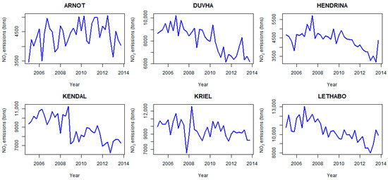
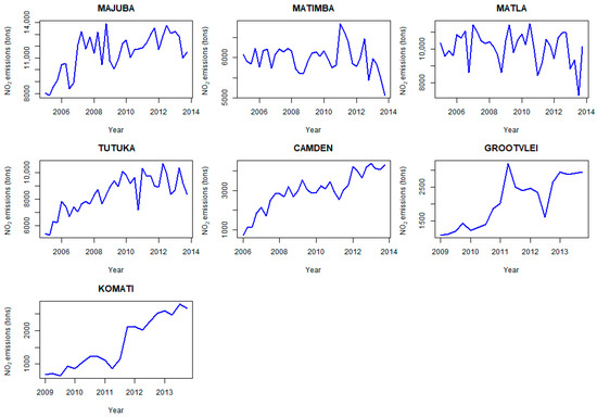
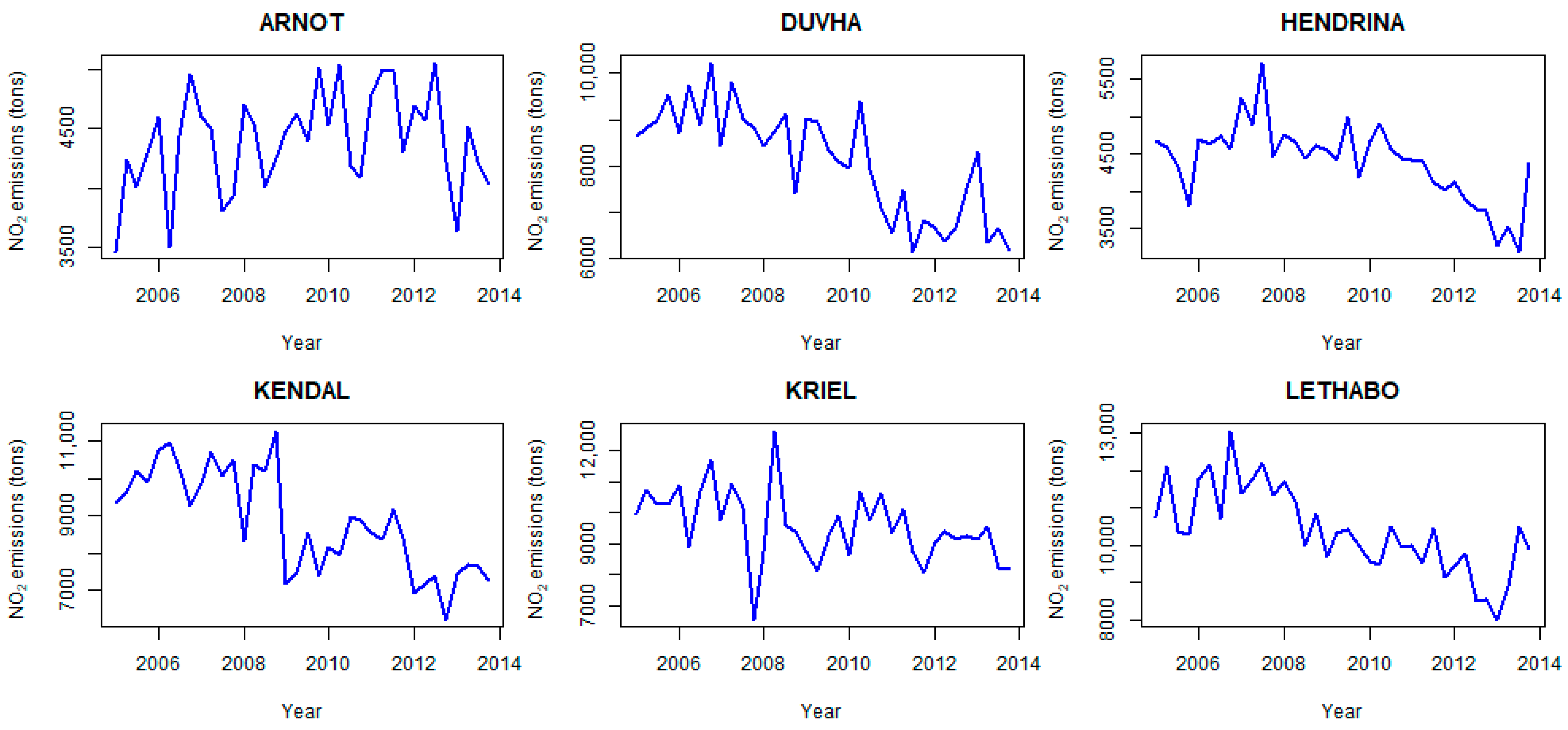
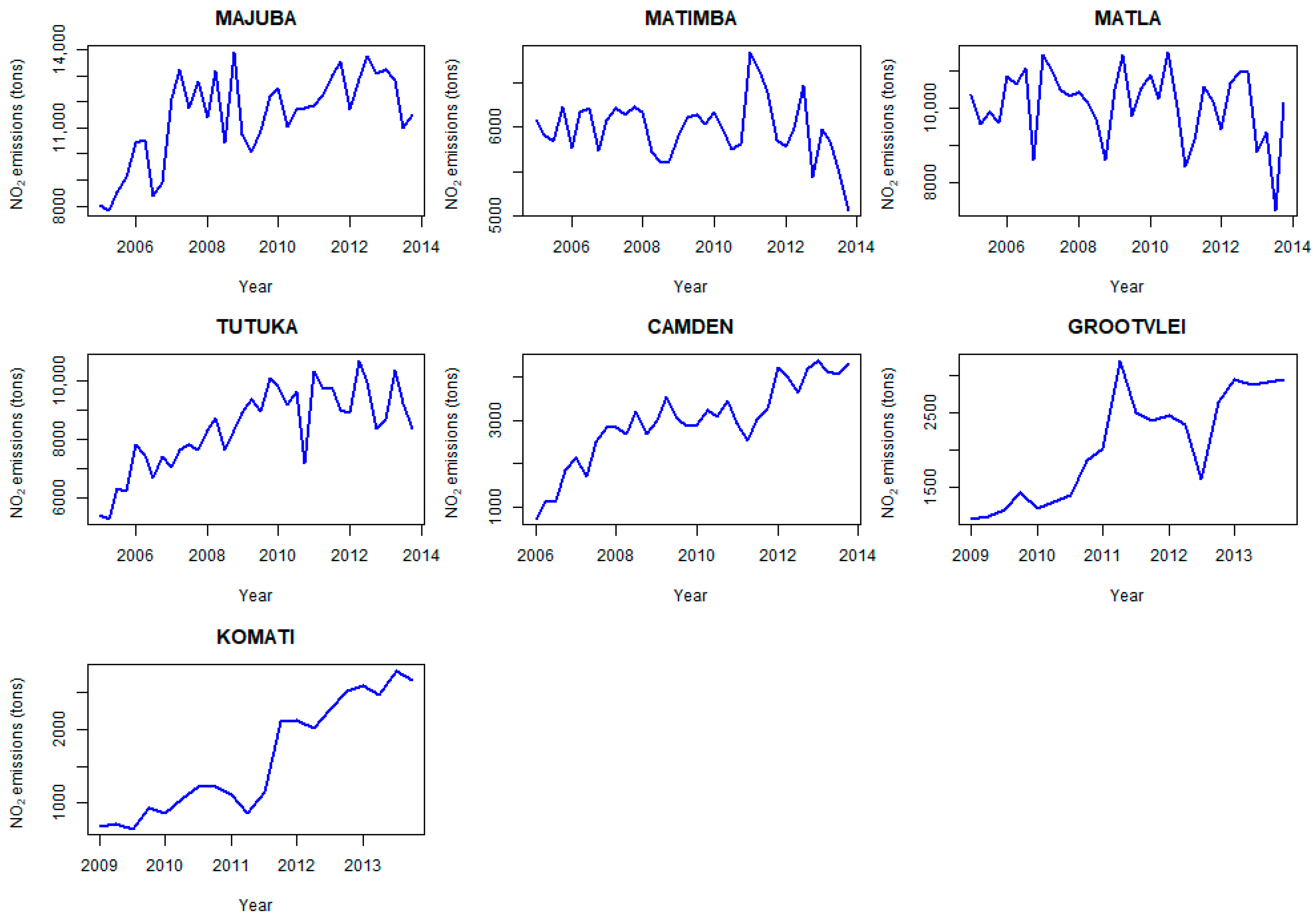
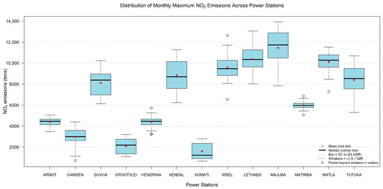
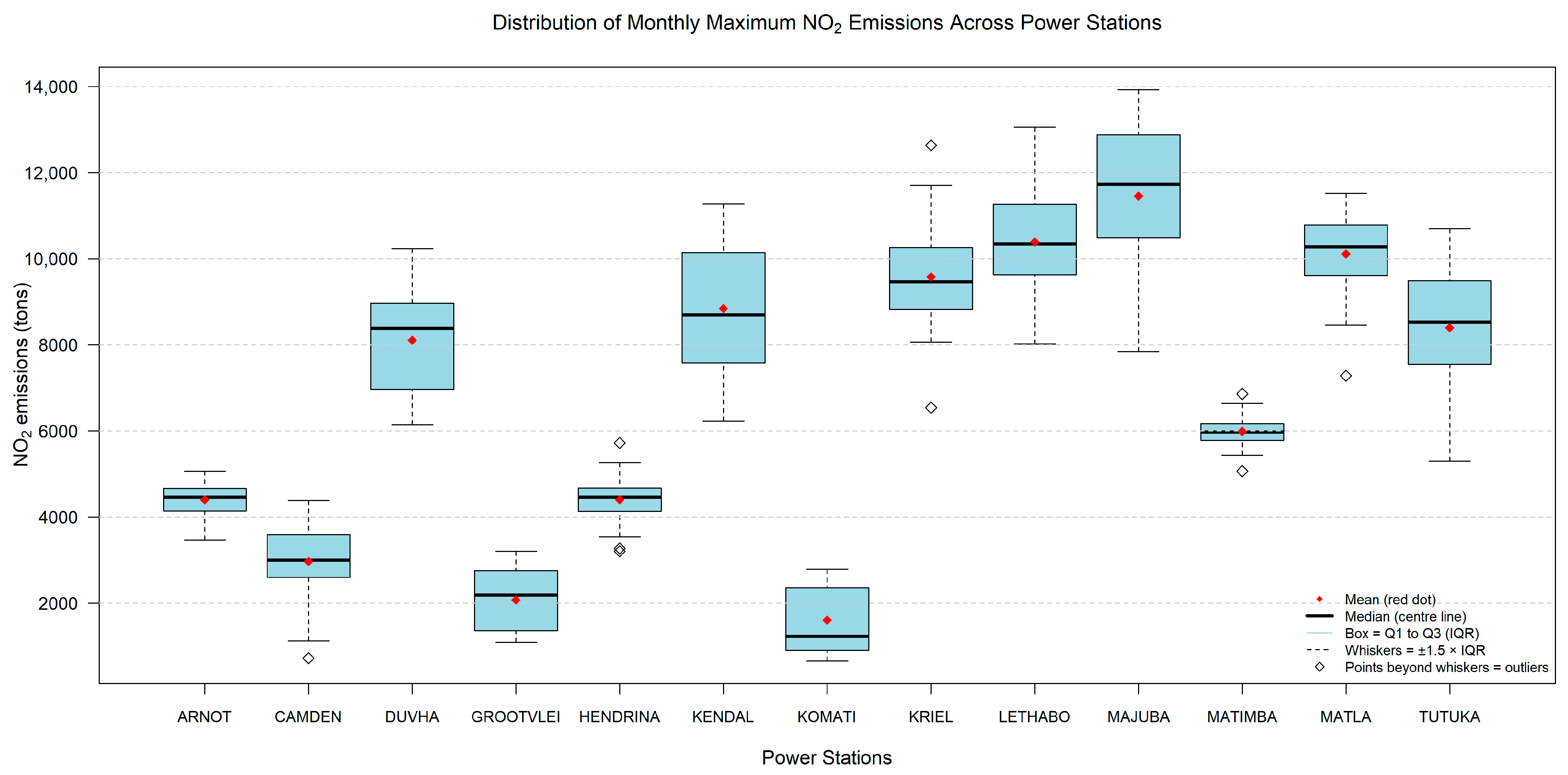
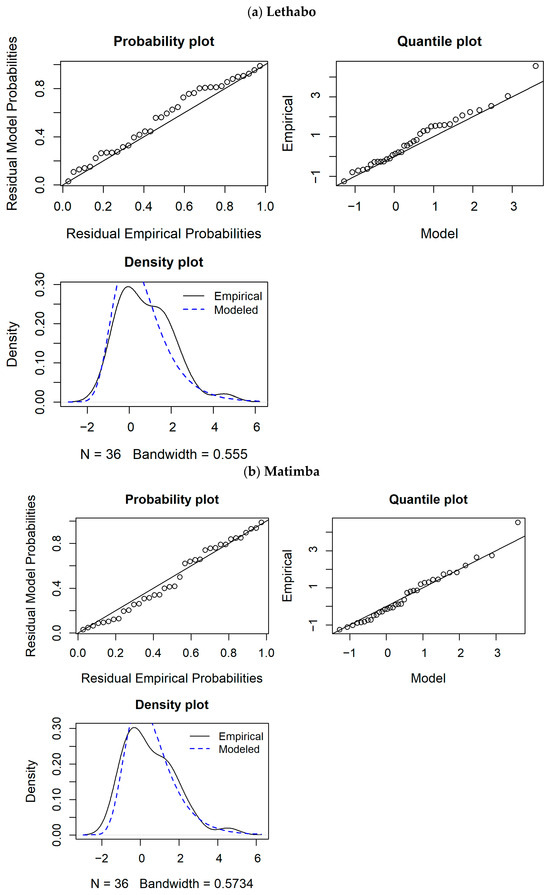
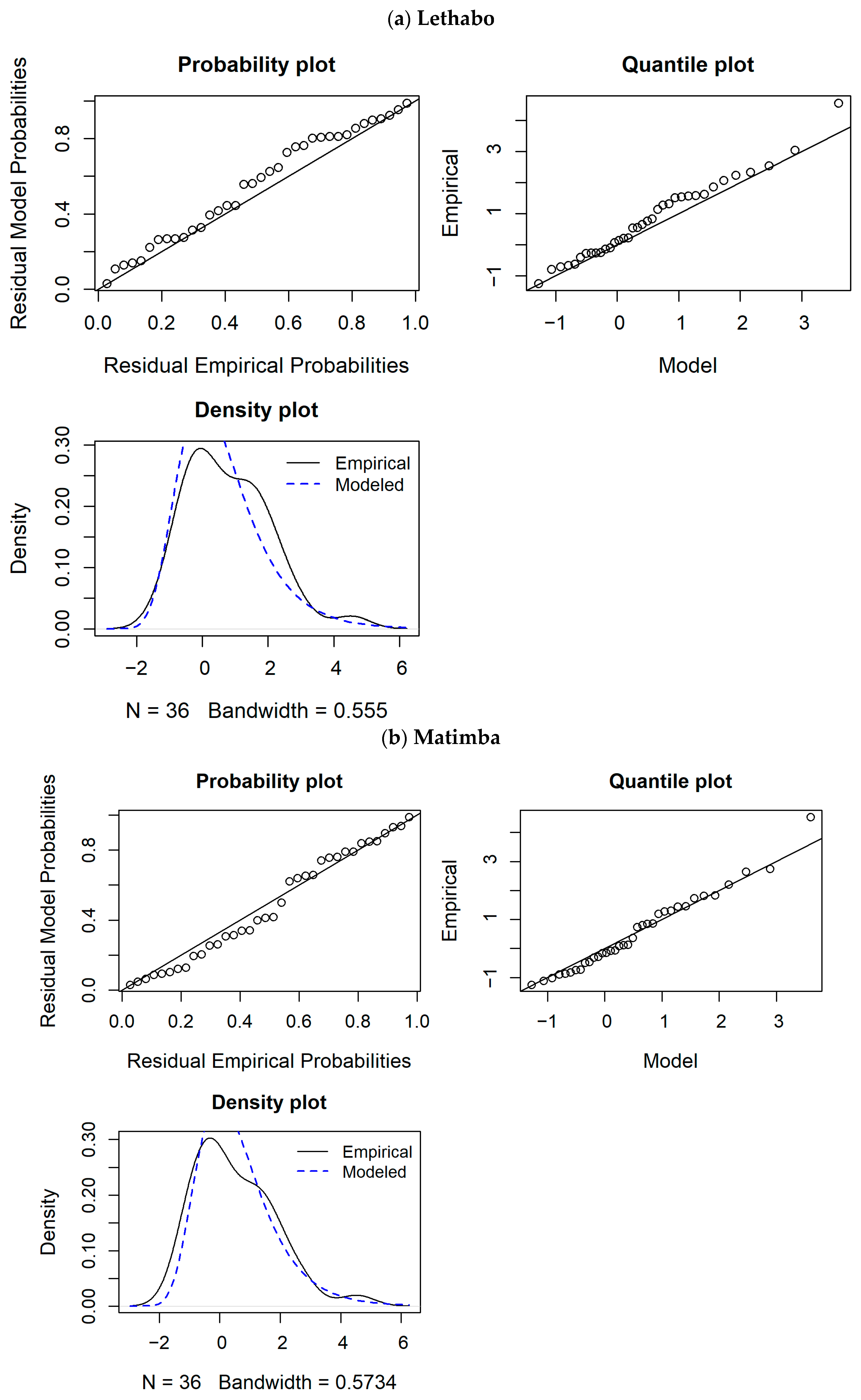

Disclaimer/Publisher’s Note: The statements, opinions and data contained in all publications are solely those of the individual author(s) and contributor(s) and not of MDPI and/or the editor(s). MDPI and/or the editor(s) disclaim responsibility for any injury to people or property resulting from any ideas, methods, instructions or products referred to in the content. |
© 2026 by the authors. Licensee MDPI, Basel, Switzerland. This article is an open access article distributed under the terms and conditions of the Creative Commons Attribution (CC BY) license.