


Abstract
This study investigates microclimatic variation across four environmentally and socially vulnerable neighborhoods in Philadelphia, utilizing ground-based measurements to assess urban heat (UH) and heat stress (HS). HS metrics, specifically Wet-Bulb Globe Temperature (WBGT) and heat index (HI), were calculated from UH measurements, including dry bulb and globe temperature, relative humidity, and wind speed. The methodology incorporates statistical modeling to identify significant predictors of HS, with street orientation (north–south and east–west) emerging as a key determinant, while categorical shade conditions were not statistically significant. Notably, Kingsessing exhibited lower HS and a unique humidity profile, whereas temperatures in Point Breeze and Grays Ferry and Hunting Park were consistently elevated. The research demonstrates that neighborhood-scale measurements can reveal critical spatial differences in UH and HS that are helpful in customizing mitigation strategies to specific communities. The approach is adaptable for integration with public health and emergency response initiatives, supporting data-driven decision-making for local governments and community-based organizations. Although assessment of physiological metrics and sampling during peak heat periods were not possible, overall, the study provides a practical framework for addressing urban heat vulnerability and underscores the importance of context-specific, community-engaged solutions to protect at-risk populations from extreme heat impacts.
1. Introduction
Relative to extra-urban baselines, the urban heat island (UHI) effect can lead to high urban heat (UH) and associated heat stress (HS). This physiological strain can inhibit the body in maintaining a stable internal temperature, subsequently creating negative human health outcomes, and other negative impacts on the economy and wildlife [1,2,3,4]. The intensities of UH and UHI are determined by a variety of factors, including anthropogenic heat emissions, the thermal behavior of built materials, urban morphology, and the extent of green canopy [5,6]. Temporally, UH and UHI follow distinct daily cycles: while UH generally peaks during the day when ambient air temperatures are at their absolute highest, the UHI effect—which quantifies the difference in temperature between urban centers and surrounding rural areas—usually reaches its maximum intensity after dusk and throughout the night [7].
Measuring HS is difficult because it is determined by a variety of behavioral, physiological, and environmental elements [8]. Heat researchers utilize more than 40 distinct heat indices, with each approach carrying its own unique set of strengths and drawbacks [9]. Broadly speaking, these indices fall into three primary categories: rational indices derived from heat balance models, empirical indices which are founded upon “objective and subjective strain,” and direct indices that rely on the immediate observation of localized environmental conditions [10].
Two of the most common directly measured indices are the heat index (HI) and the Wet-Bulb Globe Temperature (WBGT). The HI is derived from the relative humidity and ambient air temperature and is intended to simulate the perceived thermal experience of humans [11]. An “excessive heat warning” is triggered by the United States National Weather Service (NWS) if the HI is forecast to reach or exceed 40.56 °C for a minimum of two consecutive days, provided nighttime temperatures remain above 23.89 °C [12].
The WBGT is derived empirically from the natural wet-bulb temperature (Tw), the globe temperature (), and the dry-bulb temperature (). Specifically, Tw captures the impact of short- and long-wave radiation absorption, utilizing a wetted thermometer to mimic the human body’s evaporative cooling process [11]. Reaching a Tw limit of 35 °C is critical, as it constitutes a lethal threshold if endured for six hours [2]. Meanwhile, is derived from a combination of solar radiation, wind speed, and air temperature, designed to emulate the thermal response of human skin to these environmental variables. Finally, simply represents shaded, ambient air temperature [12].
While widely endorsed for assessing outdoor conditions, the WBGT lacks extensive empirical validation in urban microclimates. Historically, its application began in the 1950s within U.S. military training camps to mitigate exertional heat-related illnesses [13]. Also subject to the UHI effect, urban WBGT values generally exceed those of surrounding rural landscapes [1].
As urbanization proceeds, UH rises, and UHIs expand, strategies for alleviating HS have become of increasing interest to researchers. Individuals can mitigate HS through simple actions like drinking water, bathing, or seeking indoor shelter during the hottest parts of the day [14]. Yet, for where UH is highest, these individual coping mechanisms may be inadequate. In dense urban environments without extensive vegetative canopies, ref. [15] describes shade as a frequently underestimated approach to reducing HS, capable of dropping an individual’s net thermal load by an impressive 20 to 40 °C. Economically disadvantaged urban communities often have the least shade, with profound racial disparities in HS exposure also reported refs. [16,17].
Research has documented how different forms of shade—including architectural features, vegetated canopies, and artificial structures—cool the immediate environment, though research specifically tracking HS indices remains sparse. For instance, ref. [18] evaluated shading as a thermal-reduction tactic in Tempe, Arizona, utilizing high-resolution thermal imaging alongside 3D urban models and land cover data. Their findings revealed that environments shaded by trees experienced significantly lower temperatures than those shaded by man-made structures, with the cooling benefits proving to be additive. In another study, ref. [19] contrasted the cooling power of natural trees against artificial sun sails in Pécs, Hungary. Their results demonstrated that suspended sun sails positioned just above street level were inferior to natural tree canopies for alleviating local HS. Trees successfully lowered the physiological equivalent temperature (PET), an index evaluating thermal comfort by correlating outdoor climates with corresponding indoor conditions [20]. To illustrate, PET measurements under trees hovered between 25 and 34 °C, while areas beneath the sun sails registered hotter PET ranges of 29 to 36 °C.
Ref. [21] tested a specialized framework to optimize tree placement for UH reduction by combining tree physical characteristics with urban geometric properties (specifically using the sky-view factor, or SVF, to quantify the amount of sky visible from the street canyon). This model demonstrated that while trees boasting dense foliage are generally superior at cooling, their exact positioning is paramount; heavily foliated trees deliver the greatest benefits in sun-exposed gaps between buildings and offer diminishing returns if planted in already shaded zones. Ref. [22] examined the relationship between various UH metrics, street alignment, and tree canopy abundance in Melbourne, Australia. The results indicated that in heavily canopied corridors, streets running east-to-west achieved more substantial drops in air temperature than those running north-to-south.
Some of these studies utilized HS indices to quantify differences. Ref. [21] examined comfort indices; ref. [22] examined multiple microclimate variables, including temperature, humidity, and radiation; and ref. [20] considered PET in a somewhat specialized context—that of a half-marathon race. Of these studies, only ref. [19] considered both HI and WBGT, albeit in a somewhat narrow context, comparing the effectiveness of trees and sun sails. None of these studies considered more general predictors of both HI and WBGT variation over different neighborhoods of a city.
Though significant UH differences can be found within the same city [23,24], measurements of microclimatic differences in cities remain scarce [25]. Neither urban weather stations nor remote sensing provide sufficient spatial resolution to characterize intra-urban trends. Geostatistical models can predict general trends but have less precision in assessing the impacts of small-scale topographic features [26]. Ref. [27] found that both vegetation and building characteristics influence UH and that differences among parts of the same urban area are greater at night than during daytime. Ref. [28] explored the personalized heat strain endured by outdoor public safety and groundskeeping personnel stationed in Charleston, South Carolina. By correlating individual HI exposure (IHIE) alongside established weather station HI and UHI data, the research revealed that personal exposure levels aligned closely with local weather station metrics yet showed distinct deviations from standard 2021 UHI calculations. In a separate validation effort, ref. [29] tested the precision of three distinct WBGT forecasting frameworks: NOAA’s Southeast Regional Climate Center (SERCC), Carolina’s Integrated Science and Assessments (CISA), and the NWS, by benchmarking them against actual field-measured WBGT conditions. Their analysis demonstrated that the CISA and SERCC tools outperformed the NWS framework, indicating that macro-level models frequently deployed for public heat warnings often miss the subtle, localized microclimate variations existing across a cityscape. To capture these granular gradients, contemporary research has increasingly adopted mobile tracking equipment mounted on pedestrians, bikes, or cars to log spatial microclimatic shifts [30], although this methodology is still emerging. Ultimately, while ref. [28] concentrated solely on the HI and ref. [29] isolated WBGT, neither research effort attempted to evaluate both of these critical metrics simultaneously.
To prioritize urban heat mitigation efforts, spatiotemporal differences in microscale UH and HS need to be better understood [7]. This study addresses this need with ground-level measurements of UH and HS in four different neighborhoods of Philadelphia, Pennsylvania (USA). Key research questions addressed include: how much spatial variability in UH and HS can be measured? Do different metrics of UH and HS give similar information? How do urban morphological features causing different shade patterns influence UH and HS? To evaluate how thermal conditions evolve over time, stationary sensors concurrently recorded UH and HS in each neighborhood. To evaluate spatial differences, trained community volunteers simultaneously conducted a mobile measurement campaign of these same variables on city blocks with different orientations and shade status. We hypothesize first that statistically significant differences in both UH and HS can be observed, and second, that the intensity of HS is correlated with street orientation and shade status.
2. Materials and Methods
2.1. Project Background and Goals
Data acquisition began during the late spring and summer of 2020, the first summer of the COVID-19 pandemic. At the project’s inception, official and unofficial cooling centers—such as swimming pools, libraries, senior centers, and shopping centers—were closed. Measurements began in the spring of 2020 in the Hunting Park section of north Philadelphia. Over the following four summers, additional measurements were taken in four other Philadelphia neighborhoods: Haddington, Kingsessing, and Point Breeze/ Grays Ferry. The academic members of the research team worked in close partnership with community-based organizations (CBOs) based in each study neighborhood. Additional information regarding the study design can be found in [31].
2.2. Neighborhood Descriptions
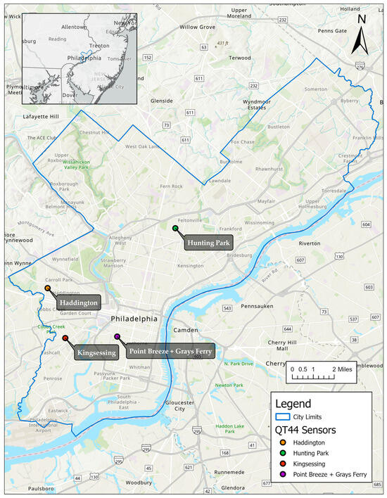
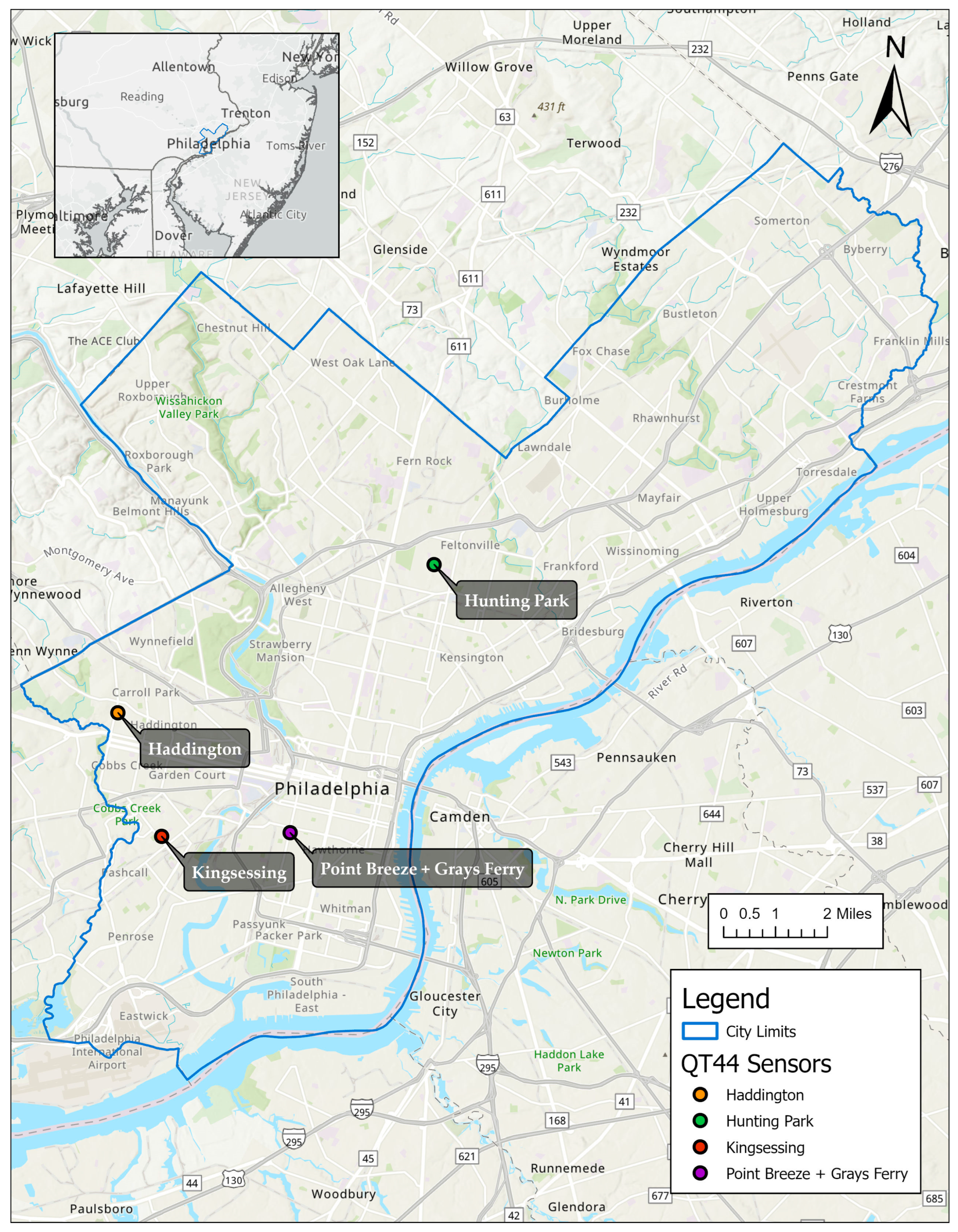
The study was conducted across the four neighborhoods, as illustrated in Figure 1, each of which was identified as an environmental justice community [32]. Demographic characteristics of each neighborhood and the entire City are presented in Table 1. “Neighborhoods” were defined using locally recognized community boundaries that reflect socially and institutionally recognized distinctions rather than any formal administrative boundaries. Neighborhood area and population estimates were calculated by aggregating the most recent American Community Survey (ACS) 5-year census tract data corresponding to these boundaries. Tree canopy coverage was derived from publicly available City of Philadelphia urban tree canopy datasets and summarized within each neighborhood boundary to characterize relative vegetative cover.
Figure 1.
Neighborhood locations. The points show the sites of the stationary QUESTemp° 44 monitoring devices, which served as the starting points for the mobile data collection.
Table 1.
Characteristics of the four neighborhoods, compared with citywide baselines. Demographic metrics from [33,34] and tree canopy coverage from [35,36].
2.3. Fixed Measurements
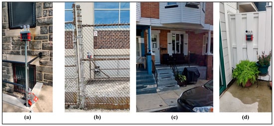
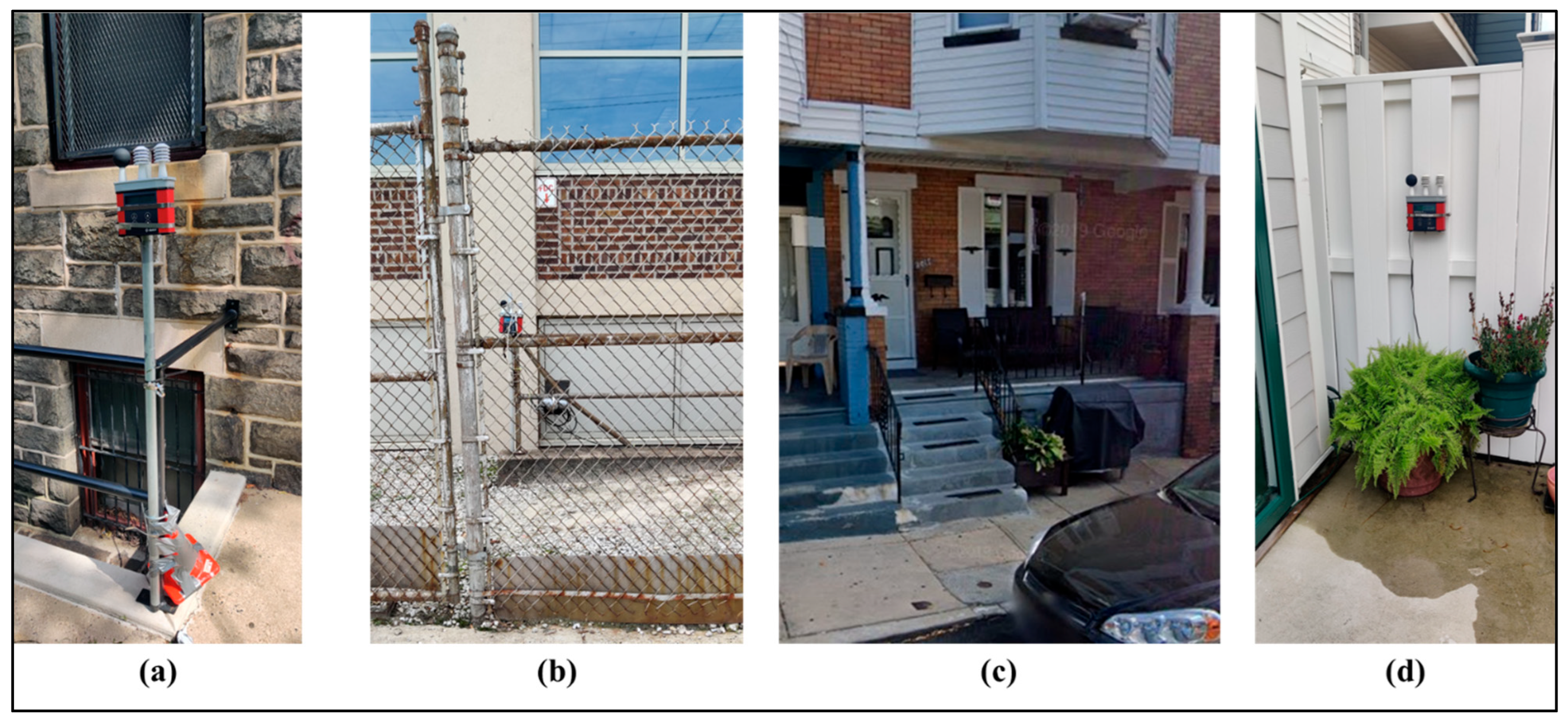
To measure temporal variations in UH and HS, a single QUESTemp° 44 (QT44) monitoring device was deployed in each of the four neighborhoods. Sampling at ten-minute intervals, the QT44 recorded , , and relative humidity (RH), providing the foundational data required to subsequently calculate Tw, WBGT, and HI. The locations of the QT44 units are mapped in Figure 1 and pictured in Figure 2. The specific locations were selected to minimize the chance of vandalism, to ensure access to a power supply, and to avoid exposure to extreme wind and solar radiation. Following the manufacturer’s specifications, each QT44 was installed 1–2 m above the local ground elevation to emulate thermal exposure by pedestrians.
Figure 2.
Deployment sites for the stationary QUESTemp° 44 monitoring instruments across the four evaluated districts: (a) Haddington, (b) Hunting Park, (c) Kingsessing, and (d) Point Breeze and Grays Ferry.
2.4. Mobile Measurements
To measure spatial differences in UH and HS, trained citizen scientists used Kestrel 5400 (Kestrel Instruments, Nielsen-Kellerman, Boothwyn, PA, USA) to make mobile measurements at designated waypoints along predetermined walking routes. The Kestrel devices were used to measure wind speed, RH, and WBGT on weekdays during the peak thermal window of 11:00 to 14:00. (Detailed guidelines provided to the citizen scientists can be found in ref. [31]).
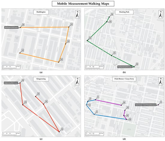
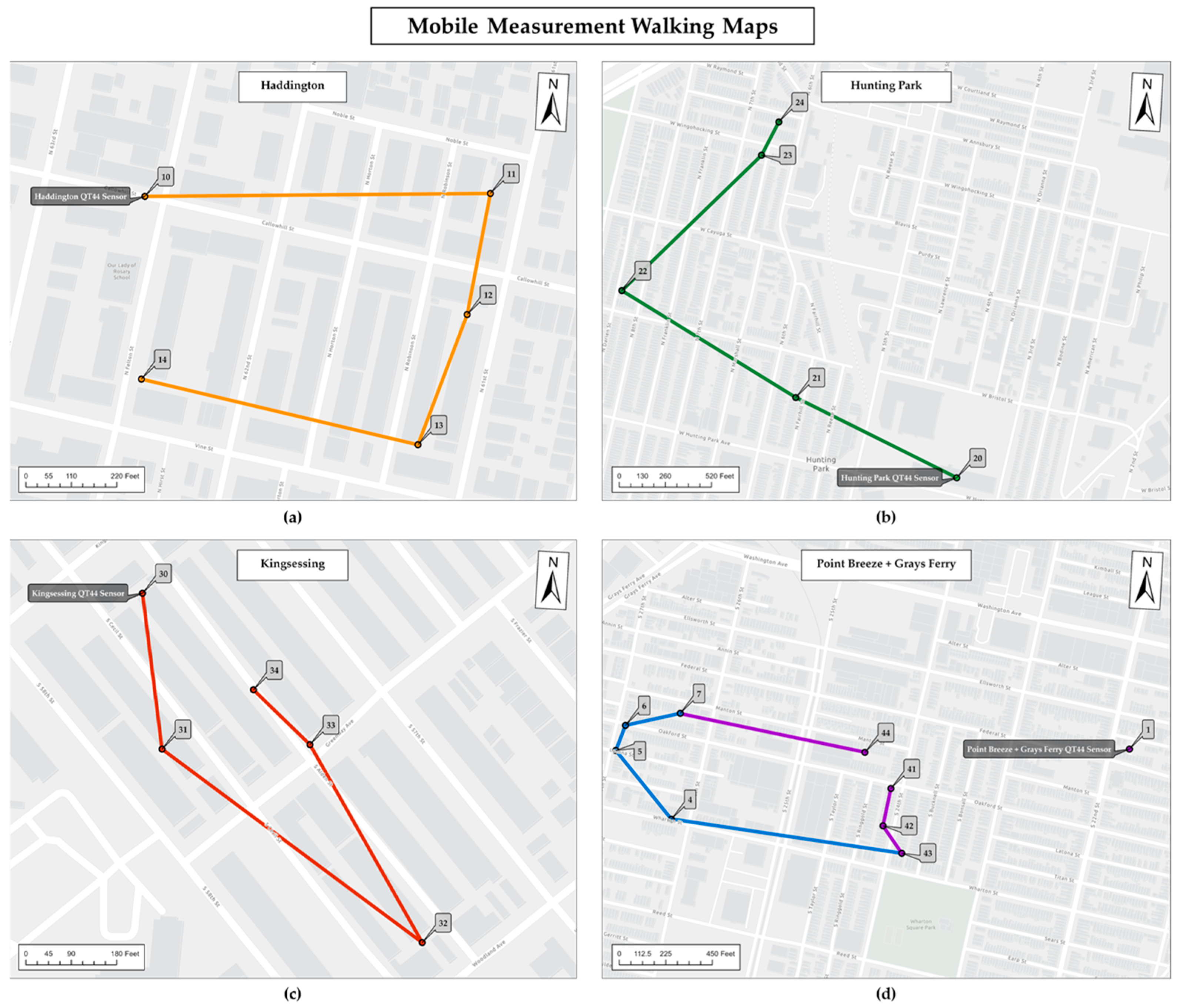
Within each neighborhood, measurements were made at twenty locations along the routes (Figure 3). The research team carefully chose these locations to sample a variety of shade conditions and street orientations. A comprehensive breakdown of these 20 sites and their specific shade and orientation classes is provided in Table 2. The shade conditions of each location were classified as “no shade”, “partial shade”, or “full shade” based on the tree canopy shown both in aerial imagery sourced from Google Maps (2023) and photos taken by the research team at each site [31]. Locations featuring a heavily foliated tree were labeled as “full shade”; those with a sparsely leafed tree or partial canopy fell under “partial shade”; and sites completely devoid of trees were categorized as “no shade”. It is important to note that the shade classification was based only on tree canopy and did not consider other sources of shade.
Figure 3.
Pedestrian routes deployed by citizen scientists for gathering mobile environmental data. Detailed route schematics are shown for (a) Haddington, (b) Hunting Park, (c) Kingsessing, and (d) Point Breeze and Grays Ferry (specifically covering monitoring stations 4 to 7, 41 to 43, and 48).
Table 2.
Data collection sites.
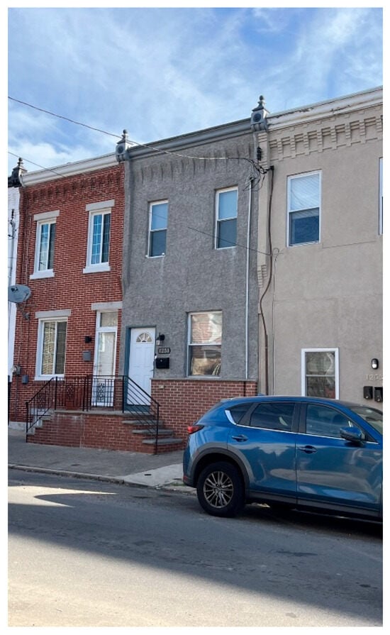
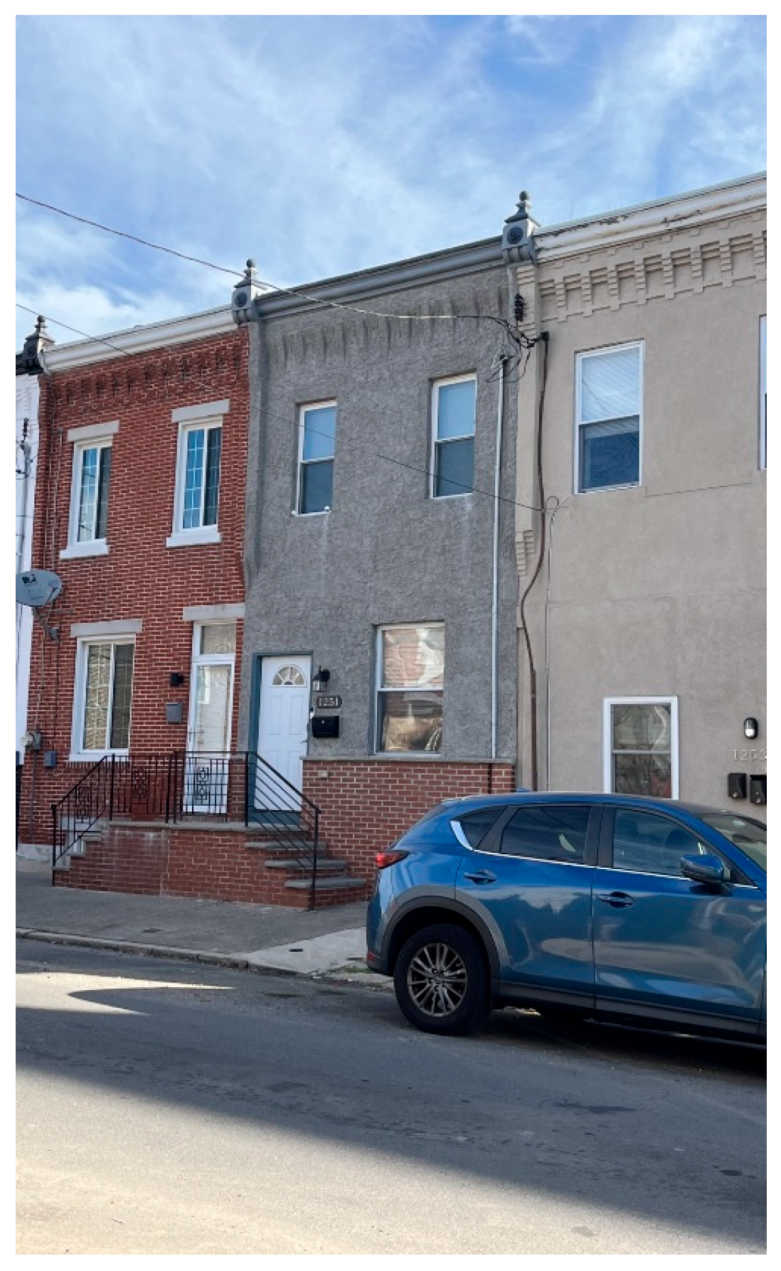
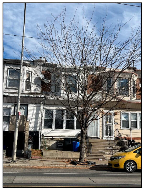
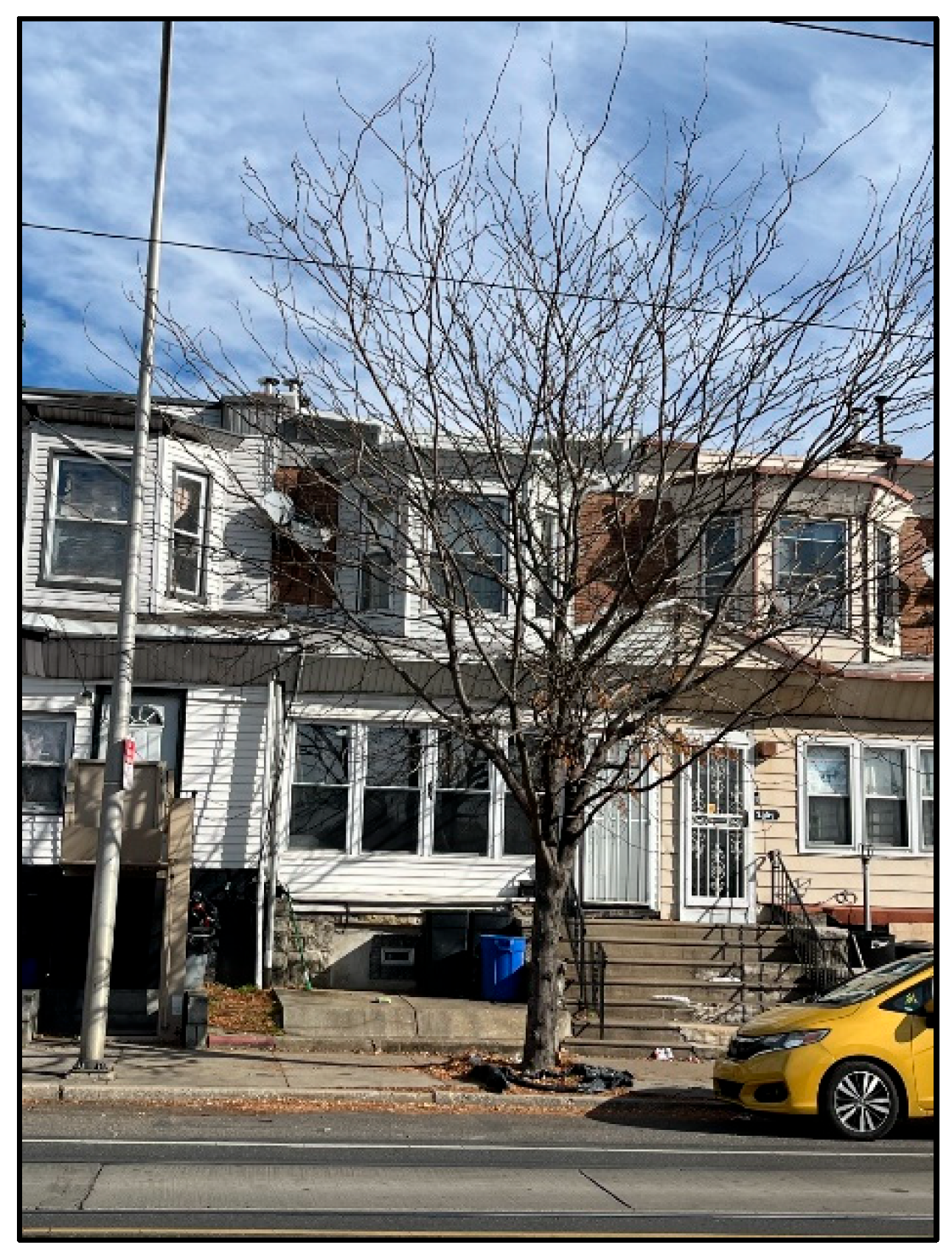
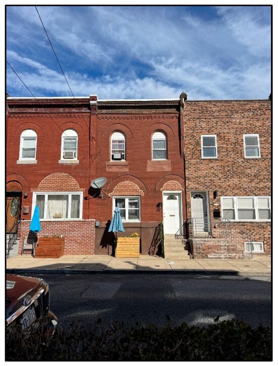
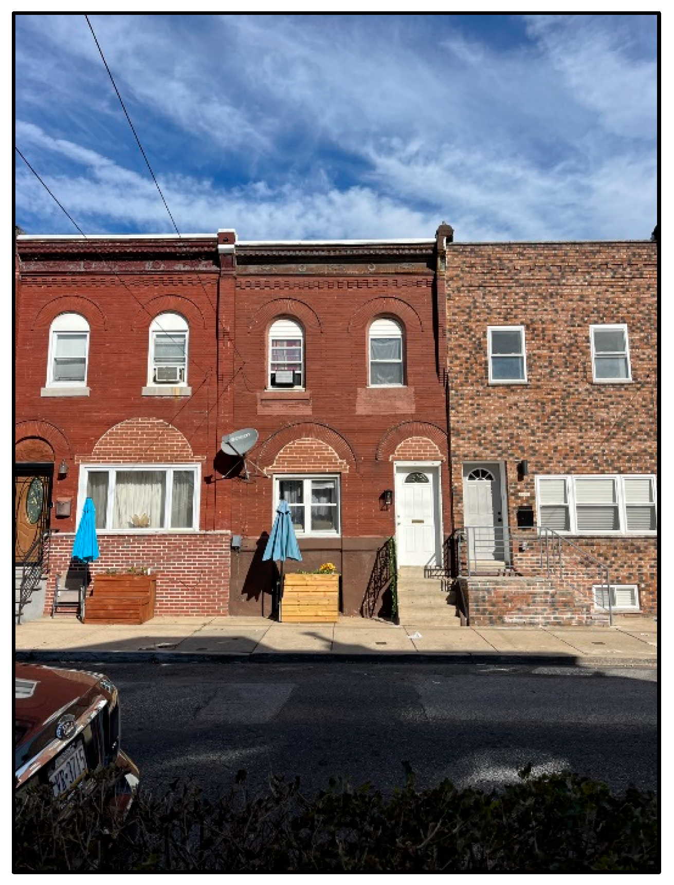
In Hunting Park, Haddington, and Point Breeze and Grays Ferry, street orientation was either north–south (NS) or east–west (EW). Kingsessing was unique in that its streets are oriented as either north-east (NE) or south-west (SW). Each measurement location was also assigned a unique “location ID” (Figure 3). Photographs of three of the monitoring locations are provided in Figure 4, Figure 5 and Figure 6.
Figure 4.
Point Breeze and Grays Ferry Monitoring Site 5, located at 1251 South 27th Street, Philadelphia, PA 19146. This specific measurement spot is positioned along a north–south roadway completely devoid of tree canopy (classified as “no shade”). The photograph was captured on 2 November 2023.
Figure 5.
Photo of Kingsessing Location 31, captured on 2 November 2023.
Figure 6.
Photo of Point Breeze and Grays Ferry Location 48, captured on 2 November 2023.
2.5. Normal Testing
Using IBM SPSS Statistics (Version 29) (SPSS), normal p-p plots (probability plots of standardized regression residuals) were developed to assess the distribution of each HS metric. HI exhibited normally distributed residuals, but WBGT did not. To normalize the WBGT residuals, a logarithmic transformation was applied to the WBGT data, and the natural logarithm of WBGT, denoted as ln(WBGT), became the primary dependent variable used in subsequent regression models.
2.6. Urban Heat Stress Metrics and Gaps in Data Collection
UH is determined by , , RH, and wind speed. The latter two variables were measured directly using the Kestrel sensors, while and were measured by the closest QT44. Specifically, the and values corresponding to each mobile measurement were estimated assuming linear interpolation between the QT44 measurements that immediately preceded and followed the mobile time stamp.
In instances where QT44 equipment failed to record data—such as during a loss of battery power—ambient air temperatures logged by the National Weather Service gauge at the Philadelphia International Airport (Network ID: GHCND:USW00013739) served as a proxy. This data substitution was only applied to the Haddington site on 22 August and the Kingsessing location on 23, 24, and 28 August.
The specific dates for which the stationary and mobile data were analyzed are provided in Table 3. Mobile measurements were collected across all four neighborhoods on seven days (e.g., 15–17, 22–24, and 28 August). Stationary monitoring occurred continuously over a ten-day period (e.g., 15–19 August and 30 August–3 September).
Table 3.
A comprehensive log of the specific days when data collection occurred across all four study areas using both types of monitoring equipment. An “X” marked in a cell signifies that the corresponding device was actively capturing data on that given date, whereas an empty space denotes an absence of recorded measurements for that specific instrument.
2.7. Heat Stress Metrics
As stated previously, the two HS indicators (e.g., HS and WBGT) were evaluated at every mobile data collection point. To determine the WBGT, the recorded values from both the QT44 and Kestrel devices are substituted directly into Equation (1):
To determine HI, Equations (2)–(5), which are sourced directly from the National Oceanic and Atmospheric Administration’s publication titled “The Heat Index Equation”, were used. The foundational biometeorological research for these formulas was originally conducted by [37], who developed a comprehensive matrix linking the HI to various environmental factors. Building upon this groundwork, ref. [38] refined the assessment by executing multiple regression evaluations on Steadman’s original data matrix, which ultimately yielded Equation (2):
In this formula, RH denotes the percentage of relative humidity. It is crucial to recognize that Equation (2) merely provides a baseline approximation of the HI [38], prompting the creation of several supplementary corrections—specifically Equations (3)–(5)—to improve accuracy. For instance, in scenarios where ambient temperatures range from 80 to 112 °F, and the RH drops below 13%, the following calculated value must be deducted from the initial HI:
When the temperature is between 80 and 87 °F, and the RH is greater than 85%, an additional adjustment, given in Equation (4), is made:
The second adjustment is added to the HI value from Equation (2).
In cases where HI is below 80 °F, Equation (1) and the associated adjustments are not appropriate. Instead, Equation (5) is employed:
2.8. Differences in UH and HS Among Sites
To determine whether there were differences in UH and HS across the various measurement locations, linear regression modeling was conducted using SPSS. Separate linear regression models were constructed for each dependent variable. For each model, “baseline conditions” were established as the location and date with the lowest average value for the dependent variable being analyzed. For example, when evaluating , the value measured of 31 on 23 August in Kingsessing was identified as the baseline location and time, as this baseline represented the lowest average values compared to the other dates and locations. The baseline conditions served as the reference point for all the model comparisons. The general form of the regression model is shown in Equation (6):
where Y represents either UH or HS, β0 is the intercept corresponding to the mean value at the baseline location and date, β values are the effects of locations and dates relative to the baseline, and “I” values are indicator variables for each site and date—the “Predictors”. The β values, or beta coefficients, indicate the average change in the dependent variable (UH or HS) relative to the baseline condition for each site and date. These coefficients quantify how microclimatic conditions varied across different locations and time frames. To test the impacts of differences in a location’s UH or HS compared to the baseline, the beta coefficient for a specific location was tested vs. zero, and tests with p-values <0.001 were considered statistically significant. The specific sites and dates selected as baseline conditions, and the regression results for UH, are provided in Table 4. Further results for HS regression modeling are presented in Table 5 and Table 6.
Table 4.
Significant predictor results of UH parameter models, including the corresponding beta coefficient range, when tested with each UH independent variable (“Predictors”). Non-significant predictors were omitted from the table for clarification.
Table 5.
HI significant model results, including their corresponding beta coefficients, when tested with each UH independent variable (“Predictors”). 24 August 2023 and Kingsessing site 31 constituted the baseline. Predictors without significant effects were omitted from the table for clarification.
Table 6.
ln(WBGT) significant model results, including their corresponding beta coefficients, when tested with each UH independent variable (“Predictors”). The multiplier difference in degrees Celsius was calculated for the model that assessed WBGT because the ln(WBGT) was utilized in the modeling. Baseline for the model was 24 August 2023 and Kingsessing 31. Non-significant predictors were omitted from the table for clarification.
2.9. Shading and Street Orientation
To assess the impact of shading and street orientation, a linear model was used with either the ln(WBGT) or HI as the dependent variable. The independent variables were categorical shade condition, street orientation, and date:
All variables are as defined above, except that the index variables are modified to denote the shade and street orientation. Again, the condition with the lowest independent variable values was chosen as the baseline and represented by the intercept, with differences by shading condition, street orientation, and date represented by the beta coefficients. Table 5 and Table 6 show the baseline values selected for the analyses. To assess the impact of orientation and shade condition, their respective beta values were tested vs. zero, and tests with p-values of <0.001 were considered statistically significant.
3. Results
3.1. Neighborhood Differences
The raw data collected by the two sensors utilized can be viewed in ref. [31]. To evaluate the determinants of UH, Table 4 summarizes the statistically significant predictors (p < 0.001) for the four UH indicators and their corresponding beta coefficients. These coefficients represent the expected increase in each dependent variable relative to the established baseline conditions, with date coefficients compared to the baseline date and location coefficients compared to the baseline location.
A clear pattern of neighborhood differences emerged from the analysis. Kingsessing showed the lowest levels of HS in three out of the four UH models, distinguishing itself as the only neighborhood with statistically significant differences in RH compared to the baseline. The lower values for Kingsessing suggest that this neighborhood may have unique microclimatic characteristics that influence its HS profile.
Further examination of the predictor variable revealed that neighborhoods such as Point Breeze and Grays Ferry and Hunting Park had significantly higher values than the baseline, indicating elevated HS in these areas. In contrast, most locations in Haddington and Kingsessing did not differ significantly from the baseline, reinforcing the distinctiveness of Kingsessing’s microclimate. The largest differences from the baseline were observed at sites 48 (3.9 °C), 5 (3.7 °C), and 7 (3.7 °C). Analysis across time showed that all the measurement dates, except the baseline, were associated with statistically significant differences, with 15 August 2023 showing the greatest temperature differential at 7.6 °C.
A similar trend was seen for the predictor variable, where Point Breeze and Grays Ferry again exhibited higher values, although only one location in Hunting Park reached statistical significance. The greatest differences for occurred at locations 48 (5.7 °C), 5 (6.2 °C), and 7 (5.5 °C). All the dates, except August 22 were significantly different from the baseline, with the largest difference again on August 15 (10.1 °C).
Conversely, RH and wind velocity exhibited distinct behavioral trends. Meaningful statistical variances in RH were heavily concentrated across every monitoring site in Kingsessing, along with two specific spots in Point Breeze and Grays Ferry (sites 41 and 43). The most substantial deviations were recorded at stations 31 (15.4%), 33 (15.4%), 41 (19.0%), and 42 (20.0%). Furthermore, nearly every monitored day displayed significant differences in RH —with the only exception being 22 August 2023—peaking at a maximum deviation of 26.3% on 24 August 2023. Regarding wind speed, significant deviations from the established baseline were limited to just two sites: 22 (1.6 m/s) and 23 (2.16 m/s), while no meaningful day-to-day temporal variations were detected throughout the study period.
Together, these findings highlight substantial variation in HS and related microclimatic factors across Philadelphia neighborhoods, with Kingsessing standing out for its lower HS and unique humidity profile, while Point Breeze and Grays Ferry and Hunting Park experienced consistently higher temperatures relative to the baselines.
Table 5 and Table 6 show the significant explanatory variables (p-value < 0.001) for HI and ln(WBGT), and their associated beta coefficients. Since ln(WBGT) constituted the dependent variable in the linear regression, the beta coefficients, when exponentiated, represent a multiplicative factor for the difference in degrees Celsius for each coefficient:
When compared against the established baseline, meaningful statistical variances for the ln(WBGT) metric emerged across every monitoring site within Point Breeze and Grays Ferry, in addition to a pair of stations in Haddington (sites 13 and 14) and a single spot in Hunting Park (site 22). The most substantial deviations were recorded at stations 43 and 48, which showed values 1.2 times higher when measured in degrees Celsius. Furthermore, the analysis revealed slightly more pronounced fluctuations in ln(WBGT) across the different measurement days.
Regarding HI, every single monitoring point in the Point Breeze and Grays Ferry area displayed statistically significant departures from the baseline. The maximum HI disparities occurred specifically at site 41 (an increase of 7.3 °C) and site 5 (an increase of 6.0 °C). With the exception of 22 August and 23 August 2023, every monitored date exhibited significant statistical temporal variations, peaking on 15 August 2023, with a dramatic difference of 12.9 °C.
3.2. Impact of Shade and Street Orientation on HS Parameters
The fluctuations in both the HI and ln(WBGT) in relation to the specific day of measurement and the orientation of the streets are detailed in Table 7 and Table 8. Similarly to previous analyses, these summaries display the statistically meaningful variables alongside their corresponding beta values. Furthermore, Equation (8) was applied once more to convert the ln(WBGT) regression output into a practical temperature multiplier expressed in degrees Celsius. The statistical evaluations confirm that both primary dependent metrics are significantly influenced by temporal factors and street orientation. While day-to-day environmental shifts naturally account for a slightly larger portion of the observed variance, the physical alignment of the streets remains a crucial and statistically valid determinant of overall HS.
Table 7.
HI significant model results, including their corresponding beta coefficients, when tested with each shade and street orientation independent variable (“Predictors”). Baseline conditions: 24 August 2023 (date), NE (orientation), partial shade (shade). No significant effects detected for shade (all p > 0.001).
Table 8.
ln(WBGT) significant model results, including their corresponding beta coefficients, when tested with the shade and street orientation independent variables (“Predictors”). The multiplier difference in degrees Celsius was calculated for the model that assessed WBGT because the ln(WBGT) was utilized in the modeling. Baseline conditions: 24 August 2023 (date), NE (orientation), partial shade (shade). No significant effects detected for shade (all p > 0.001).
Our findings indicate that varying shade levels did not statistically influence either of the measured HS indices, though both metrics demonstrated equivalent day-to-day fluctuations. Moreover, streets oriented along standard cardinal axes (specifically north–south and east–west) exhibited statistically meaningful deviations compared to streets positioned diagonally (south-west and north-east).
4. Discussion
The results suggest that there are small-scale spatial differences in UH and HS. The results of the regression models presented in Table 6, Table 7 and Table 8 are summarized in Table 9 for the six dependent variables. The summary table demonstrates that when a significant difference is observed at one location within a neighborhood, it is often mirrored across all the locations in that neighborhood.
Table 9.
The results of the models run to assess spatial differences, indicating the independent variables that had significant differences (indicated with an “X” within the cell).
The research identified meaningful statistical variations linked to street orientation, whereas the designated shade categories yielded no such impacts. Detailed in Table 7 and Table 8, both north–south and east–west street configurations emerged as substantial determining factors for HS. Specifically, north–south alignments were associated with peak HI scores, while east–west layouts corresponded with the maximum WBGT readings. Furthermore, across both the HI and WBGT evaluations, the diagonal street alignments (such as SW) either showed no significant statistical deviation or served as the foundational baseline for the regression models, effectively representing the minimum recorded HS values. Ultimately, a key finding is that streets laid out on diagonal axes, relative to the cardinal directions, generally experience comparatively lower levels of overall HS.
These findings are reinforced by the neighborhood-level evaluations. As detailed in Table 7 and Table 8, the specific monitoring sites within Kingsessing generally served as the regression baseline or exhibited no statistically meaningful variances (with relative humidity being the sole exception). The street grid in Kingsessing is entirely situated on a diagonal axis compared to standard cardinal points. These findings are consistent with the conclusions of [21], suggesting that prioritization of cooling interventions could be tailored to site-specific geographic variables, including street orientation. However, in this study, street orientation is inextricably linked to a particular neighborhood. Consequently, this research cannot conclusively determine whether the observed HS discrepancies stem strictly from street orientation or other neighborhood-specific characteristics.
Additionally, the recorded HS levels may have been amplified by the interplay between the alignment of the street and the specific solar angle during the data collection window. Previous investigations by ref. [22] using PET as an indicator of HS, demonstrated that east–west streets experienced higher thermal loads compared to north–south ones. The discrepancies between our findings and those reported in ref. [22] might be explained by differences in sampling schedules or the specific sidewalk chosen for data collection. For example, monitoring site 5 in Point Breeze and Grays Ferry (depicted in Figure 4) is situated on the eastern sidewalk of a north–south aligned roadway. Consequently, during afternoon sampling sessions, this specific measurement coordinate would be subjected to direct, unshielded solar radiation.
As outlined in Table 7 and Table 8, the assigned shade classifications failed to yield any statistically meaningful variations across either evaluated heat stress metric. This absence of a clear correlation might be an artifact of how the shading categories were originally defined. The research team established these classifications by analyzing Google Maps Street View data alongside static photographs captured at every individual measurement waypoint (provided in [31]). Consequently, the real-time canopy cover present during the actual physical sampling might have deviated from the visual evidence preserved in those images. A prime example is Haddington Location 14, which received a “partial shade” designation based strictly on its corresponding site photograph (available in [31]). It is entirely possible that the local foliage cast a much denser shadow during the active data collection hours, a variable impossible to verify due to the specific timestamp of the reference photo. Because of these methodological constraints, our conclusions regarding canopy impact diverge from the broader literature, such as the work of [14,15], which successfully correlated increased shade with a reduction in heat stress.
Specific monitoring sites frequently emerged as the baseline parameters, representing the absolute minimum predicted output for a given dependent variable, across several UH and HS regression evaluations. Notably, Kingsessing site 31 had the lowest average values across both evaluated HS indicators. As depicted in Figure 5, this particular station is positioned on a Southwest-aligned thoroughfare beneath partial canopy cover, and it functioned as the foundational baseline coordinate for four of the six neighborhood variation models analyzed (specifically for , , ln(WBGT), and HI).
Conversely, station 48 in the Point Breeze and Grays Ferry district (illustrated in Figure 6) is situated along an east–west traffic corridor completely lacking canopy cover (categorized as “no shade”). This specific site stood out as a highly significant predictive variable across four of the six spatial assessment models (again, for , , ln(WBGT), and HI).
The comprehensive evaluation of street orientation and canopy impacts revealed that diagonal street grids consistently maintained cooler thermal profiles compared to their standard north–south or east–west counterparts. This observed cooling trend along diagonal avenues offers a highly plausible explanation for why Kingsessing Location 31 repeatedly served as the mathematical baseline in the majority of our regressions. Meanwhile, Location 48 in Point Breeze and Grays Ferry lies on an east–west axis. Given the solar trajectory over the course of the day, east–west corridors are subjected to prolonged durations of direct solar radiation. This sustained sunlight exposure likely accounts for the substantial deviations recorded in both the UH and HS metrics at this specific Point Breeze and Grays Ferry coordinate.
Multiple researchers recognize the importance of better characterizing spatiotemporal differences in the urban microclimate [26,27]. The present research is novel in its use of multiple, continuous in situ measurements to characterize spatial differences in UH and HS. This data-driven approach differs from other studies that use physiological and sociological indices [19,23], geospatial modeling [18,26], computational fluid dynamics [21], or vehicle-based monitoring campaigns [30].
The research supports the findings of refs. [24,27] who found that intra-urban variability in air temperature is significant. Our finding of a relationship between street orientation and UH supports the findings of ref. [27] who found that thermal comfort can be improved through intentional 3D arrangements of the urban microclimate, and ref. [21] who propose a “right tree, right place” approach for UH mitigation. Our finding that streets oriented diagonally presented lower HS compared to streets oriented in the cardinal directions differs somewhat from the findings of ref. [22] who found that reductions in air temperature due to shading were greater for E-W streets than for N-S streets.
Overall, this research provides a case study in how to identify intra-urban microclimatic differences and assess the impacts of urban form, specifically street orientation and shade, on UH and HS using spatially resolved ground-level observations. The results may well be specific to Philadelphia, and even to the neighborhoods studied in Philadelphia. Nevertheless, it provides a framework for assessing and mitigating growing concerns over the impacts of heat on urban areas.
5. Conclusions
This study used ground-based measurements to quantify statistically significant spatiotemporal differences in UH and HS across four Philadelphia neighborhoods. The results suggest that location plays a critical role in predicting HS. Contrary to initial expectations, shade was found to be a weaker predictor of HS than street orientation. No statistically significant differences were observed in HS metrics when evaluating the categorical shade condition. However, statistically significant differences were found for NS and EW street orientations and on specific dates. These findings highlight the potential influence of street orientation on HS.
Several limitations to this study should be noted, particularly the absence of individual physiological data, the subjective approach used to define shade status, and the limited period over which data was collected at all the locations. Personal thermal comfort is determined by both physical and behavioral variables, including wardrobe choices, underlying health conditions, and specific occupational settings (such as mandatory outdoor labor), none of which were captured here. WBGT often fails to capture the full severity of the actual HS in environments with minimal airflow and elevated moisture, where human sweat cannot easily evaporate [10]. Finally, due to logistical challenges, simultaneous stationary monitoring across all four neighborhoods was only possible on seven separate days, and crucially, these days did not coincide with the absolute hottest periods of the season. Consequently, the microclimatic dynamics during peak extreme heat events may deviate from the trends documented in this current dataset.
Future studies could utilize a more generalizable metric to characterize the shade provided by vegetation (i.e., tree canopy coverage, radius of shade provided at a specific time of day, etc.), and shade provided by other physical features could be considered. Quantifying and expanding the shading categories would allow for the analysis of shade’s potential contribution to HS. Future studies could also increase the duration of data measurement so that methods like the ones presented in this study can be utilized to assess patterns in HS throughout the year. To further investigate the contrasting variables that influence UH and HS, future research could develop paired visual models illustrating the physical microclimatic discrepancies between north–south and east–west street alignments. Furthermore, conducting comparative assessments across districts with inherently low versus high HS profiles would introduce a broader spectrum of environmental conditions, making it easier to pinpoint the specific factors driving divergent thermal outcomes. Finally, researchers could correlate the localized data gathered in this study with macro-level meteorological readings from the Philadelphia International Airport. Establishing this comparison could yield a predictive framework that bridges the gap between centralized airport data and true neighborhood-level conditions. Because the airport’s weather station provides continuous and easily accessible data, successfully modeling this relationship would allow researchers to accurately translate standard airport metrics into highly specific community heat profiles.
The methodology developed in this study offers a practical, neighborhood-scale approach for local governments and CBOs aiming to address heat-related vulnerabilities. By identifying microclimatic differences and pinpointing key factors—such as street orientation—that influence HS, city agencies and community organizations can tailor interventions to the unique characteristics of each neighborhood. For example, urban planners can prioritize changes in street design or orientation for future developments, or target specific neighborhoods for cooling interventions, such as installing shade structures or increasing vegetative cover. CBOs can use this data-driven approach to advocate for resources and design community-led heat mitigation strategies that reflect the lived experience of residents. Additionally, the methodology’s adaptability allows for integration with existing public health and emergency response initiatives, facilitating more effective communication and targeted heat safety outreach.
The results of monitoring efforts such as this will likely vary from city to city, given differences in both climate and urban form. This study provides a framework for jointly measuring UH and HS using spatially resolved ground-level measurements. It demonstrates that neighborhood-scale ground measurements can reveal important spatial differences in UH and HS, with street orientation emerging as a significant factor. The methodology provides a valuable framework for future studies to assess and address heat vulnerability, supporting the design of targeted, context-specific interventions. While there are limitations, the approach sets the stage for more nuanced, data-driven UH mitigation strategies that can better protect vulnerable communities from the impacts of extreme heat.
Author Contributions
Conceptualization, S.S. and F.A.M.; methodology, S.S., P.L.G. and F.A.M.; software, S.S.; formal analysis, S.S.; data curation, S.S.; writing—original draft preparation, S.S.; writing—review and editing, S.S., N.P., P.L.G. and F.A.M.; visualization, S.S.; supervision, F.A.M.; project administration, N.P. and F.A.M.; funding acquisition, F.A.M. All authors have read and agreed to the published version of the manuscript.
Funding
This research was funded by the William Penn Foundation (#117-21) and the National Oceanic and Atmospheric Administration (NOAA) through Supporting Regional Implementation of Integrated Climate Resilience: Consortium for Climate Risks in the Urban Northeast (CCRUN) Phase III (NA21OAR4310313).
Data Availability Statement
The original contributions presented in this study are included in the article. Further inquiries can be directed to the corresponding author.
Conflicts of Interest
The authors declare no conflicts of interest. The funders had no role in the design of the study; in the collection, analyses, or interpretation of data; in the writing of the manuscript; or in the decision to publish the results.
Abbreviations
The following abbreviations are used in this manuscript:
| HI | Heat index |
| HS | Heat stress |
| NWS | National Weather Service |
| UHI | Urban head index |
| UH | Urban heat |
| NOAA | National Oceanic and Atmospheric Administration |
| WBGT | Wet-bulb globe temperature |
References
- Fischer, E.M.; Oleson, K.W.; Lawrence, D.M. Contrasting urban and rural heat stress responses to climate change. Geophys. Res. Lett. 2012, 39, L03705. [Google Scholar] [CrossRef] [Scilit]
- Horton, R. The Science Behind Extreme Heat. Columbia Energy Exchange, 26 July 2022.
- Da Silva Espinoza, N.; dos Santos, C.A.C.; de Oliveira, M.B.L.; Silva, M.T.; Santos, C.A.G.; da Silva, R.M.; Mishra, M.; Ferreira, R.R. Assessment of urban heat islands and thermal discomfort in the Amazonia biome in Brazil: A case study of Manaus City. Build. Environ. 2023, 227, 109772. [Google Scholar] [CrossRef] [Scilit]
- Jamei, E.; Ossen, D.; Seyedmahmoudian, M.; Sandanayake, M.; Stojcevski, A.; Horan, B. Urban design parameters for heat mitigation in tropics. Renew. Sustain. Energy Rev. 2020, 134, 110362. [Google Scholar] [CrossRef] [Scilit]
- Lin, X.; Cui, Y.; Hao, S.; Zhu, C.; Zhang, P.; Zhao, H. Influence of urban landscape pattern on summer surface temperature and its spatial scale effects. Geocarto Int. 2024, 40, 2441370. [Google Scholar] [CrossRef] [Scilit]
- Luo, T.; He, Q.; Wang, W.; Fan, X. Response of summer land surface temperature of small and medium-sized cities to their neighboring urban spatial morphology. Build. Environ. 2024, 250, 111198. [Google Scholar] [CrossRef] [Scilit]
- Martilli, A.; Krayenhoff, E.S.; Nazarian, N. Is the urban heat island intensity relevant for heat mitigation studies? Urban Clim. 2020, 31, 100541. [Google Scholar] [CrossRef] [Scilit]
- Qureshi, A.M.; Rachid, A. Review and comparative study of decision support tools for the mitigation of urban heat stress. Climate 2021, 9, 102. [Google Scholar] [CrossRef] [Scilit]
- Qureshi, A.M.; Rachid, A.; Bartlett, D. Quantifying the cooling effect of urban heat stress interventions. Int. J. Glob. Warm. 2023, 30, 60. [Google Scholar] [CrossRef] [Scilit]
- Epstein, Y.; Moran, D.S. Thermal comfort and the heat stress indices. Ind. Health 2006, 44, 388–398. [Google Scholar] [CrossRef] [Scilit] [PubMed]
- Ramirez-Beltran, N.D.; Gonzalez, J.E.; Castro, J.M.; Angeles, M.; Harmsen, E.W.; Salazar, C.M. Analysis of the heat index in the Mesoamerica and Caribbean Region. J. Appl. Meteorol. Clim. 2017, 56, 2905–2925. [Google Scholar] [CrossRef] [Scilit]
- National Weather Service. Wet Bulb Globe Temperature: How and When to Use It. 10 September 2021. Available online: https://www.weather.gov/news/211009-WBGT (accessed on 23 April 2024).
- Budd, G.M. Wet-bulb globe temperature (WBGT)—Its history and its limitations. J. Sci. Med. Sport 2008, 11, 20–32. [Google Scholar] [CrossRef] [Scilit] [PubMed]
- Aleksandrowicz, O.; Pearlmutter, D. The significance of shade provision in reducing street-level summer heat stress in a hot Mediterranean climate. Landsc. Urban Plan. 2023, 229, 104588. [Google Scholar] [CrossRef] [Scilit]
- Turner, V.K.; Middel, A.; Vanos, J.K. Shade Is an Essential Solution for Hotter Cities. Nature 2023, 619, 694–697. [Google Scholar] [CrossRef] [Scilit] [PubMed]
- Hsu, A.; Sheriff, G.; Chakraborty, T.; Manya, D. Disproportionate exposure to urban heat island intensity across major US cities. Nat. Commun. 2021, 12, 2721. [Google Scholar] [CrossRef] [Scilit]
- Chakraborty, T.C.; Newman, A.J.; Qian, Y.; Hsu, A.; Sheriff, G. Residential segregation and outdoor urban moist heat stress disparities in the United States. One Earth 2023, 6, 738–750. [Google Scholar] [CrossRef] [Scilit]
- Park, Y.; Zhao, Q.; Guldmann, J.-M.; Wentz, E.A. Quantifying the cumulative cooling effects of 3D building and tree shade with high resolution thermal imagery in a hot arid urban climate. Landsc. Urban Plan. 2023, 240, 104874. [Google Scholar] [CrossRef] [Scilit]
- Kántor, N.; Chen, L.; Gál, C.V. Human-biometeorological significance of shading in urban public spaces—Summertime measurements in Pécs, Hungary. Landsc. Urban Plan. 2018, 170, 241–255. [Google Scholar] [CrossRef] [Scilit]
- Thorsson, S.; Rayner, D.; Palm, G.; Lindberg, F.; Carlström, E.; Börjesson, M.; Nilson, F.; Khorram-Manesh, A.; Holmer, B. Is Physiological Equivalent Temperature (PET) a superior screening tool for heat stress risk than Wet-Bulb Globe Temperature (WBGT) index? Eight years of data from the Gothenburg half marathon. Br. J. Sports Med. 2021, 55, 825–830. [Google Scholar] [CrossRef] [Scilit]
- Morakinyo, T.E.; Ouyang, W.; Lau, K.K.-L.; Ren, C.; Ng, E. Right tree, right place (urban canyon): Tree species selection approach for optimum urban heat mitigation—Development and evaluation. Sci. Total Environ. 2020, 719, 137461. [Google Scholar] [CrossRef] [Scilit]
- Sanusi, R.; Johnstone, D.; May, P.; Livesley, S.J. Street orientation and side of the street greatly influence the microclimatic benefits street trees can provide in summer. J. Environ. Qual. 2016, 45, 167–174. [Google Scholar] [CrossRef] [Scilit] [PubMed]
- Alonso, L.; Renard, F. A comparative study of the physiological and socio-economic vulnerabilities to heat waves of the population of the Metropolis of Lyon (France) in a climate change context. Int. J. Environ. Res. Public Health 2020, 17, 1004. [Google Scholar] [CrossRef] [Scilit] [PubMed]
- Cao, J.; Zhou, W.; Zheng, Z.; Ren, T.; Wang, W. Within-city spatial and temporal heterogeneity of air temperature and its relationship with land surface temperature. Landsc. Urban Plan. 2021, 206, 103979. [Google Scholar] [CrossRef] [Scilit]
- Hatefnia, N.; Ghobad, M. Computing Outdoor Comfort Based on CBE Thermal Comfort Calculation for ASHRAE-55. Computational Ecologies: Design in the Anthropocene 2015. Available online: https://www.researchgate.net/publication/319351567 (accessed on 23 April 2024).
- Burger, M.; Gubler, M.; Brönnimann, S. Modeling the intra-urban nocturnal summertime air temperature fields at a daily basis in a city with complex topography. PLoS Clim. 2022, 1, e0000089. [Google Scholar] [CrossRef] [Scilit]
- Yang, C.; Kui, T.; Zhou, W.; Fan, J.; Pan, L.; Wu, W.; Liu, M. Impact of refined 2D/3D urban morphology on hourly air temperature across different spatial scales in a snow climate city. Urban Clim. 2023, 47, 101404. [Google Scholar] [CrossRef] [Scilit]
- Sugg, M.M.; Runkle, J.D.; Dow, K.; Barnes, J.; Stevens, S.; Pearce, J.; Bossak, B.; Curtis, S. Individually Experienced Heat Index in a Coastal Southeastern US City among an Occupationally Exposed Population. Int. J. Biometeorol. 2022, 66, 1665–1681. [Google Scholar] [CrossRef] [Scilit] [PubMed]
- Clark, J.; Konrad, C.E.; Grundstein, A. The development and accuracy assessment of wet bulb globe temperature forecasts. Weather Forecast. 2024, 39, 403–419. [Google Scholar] [CrossRef] [Scilit]
- Kousis, I.; Pigliautile, I.; Pisello, A.L. A mobile vehicle-based methodology for dynamic microclimate analysis. Int. J. Environ. Res. Public Health 2021, 15, 893–901. [Google Scholar] [CrossRef] [Scilit]
- Seiden, S. Quantifying Microclimatic Differences in Urban Heat and Urban Heat Stress Within Philadelphia. Ph.D. Thesis, Drexel University, Philadelphia, PA, USA, 2024. Available online: https://www.proquest.com/dissertations-theses/quantifying-microclimatic-differences-urban-heat/docview/3076815265 (accessed on 12 March 2026).
- Academy of Natural Sciences of Drexel University & City of Philadelphia. Resilient Communities Stormwater Initiative: Focus Area Map. Available online: https://storymaps.arcgis.com/stories/e76273a34b3f47798b66f256897c14eb (accessed on 12 March 2026).
- Niche. 2024 Best Places to Live in the Philadelphia Area. Available online: https://www.niche.com/places-to-live/search/best-places-to-live/m/philadelphia-metro-area/ (accessed on 23 April 2024).
- McFadden, K.; Johnson, R. Citywide Heat Ride. The Nature Conservancy StoryMaps, 6 November 2023. Available online: https://storymaps.arcgis.com/stories/1a131b1d4dd74143a47ae556809c72b3 (accessed on 23 April 2024).
- O’Neil-Dunne, J. A Report on the City of Philadelphia’s Existing and Possible Tree Canopy. 15 December 2020. Available online: https://www.phila.gov/media/20200210164446/Urban-Tree-Canopy-Report-03-18-11.pdf (accessed on 12 March 2026).
- Schmidt, S. Philly Moves Ahead with Draft Plan to Increase the City’s Green Canopy. WHYY, 1 December 2021. Available online: https://whyy.org/articles/want-more-trees-in-your-philly-neighborhood-here-is-your-chance-to-tell-city-hall/ (accessed on 23 April 2024).
- Steadman, R.G. The assessment of sultriness. Part I: A temperature-humidity index based on human physiology and clothing science. J. Appl. Meteorol. 1979, 18, 861–873. [Google Scholar] [CrossRef] [Scilit]
- Rothfusz, L.P. The Heat Index “Equation”. Available online: https://www.weather.gov/media/ffc/ta_htindx.PDF (accessed on 12 March 2026).

Disclaimer/Publisher’s Note: The statements, opinions and data contained in all publications are solely those of the individual author(s) and contributor(s) and not of MDPI and/or the editor(s). MDPI and/or the editor(s) disclaim responsibility for any injury to people or property resulting from any ideas, methods, instructions or products referred to in the content. |
© 2026 by the authors. Licensee MDPI, Basel, Switzerland. This article is an open access article distributed under the terms and conditions of the Creative Commons Attribution (CC BY) license.