


Abstract
In intermittent convective cooling environments created by split air conditioners, the dynamic nature of the environment poses challenges to traditional steady-state thermal comfort models in predicting human thermal comfort. Therefore, this study proposes an alliesthesia-informed machine learning framework that encodes alliesthesia theory into explicit mathematical features for predicting dynamic overall thermal comfort. Data were obtained through controlled experiments under intermittent cooling conditions, and a theory-driven feature set incorporating dynamic set points and physio-psycho gap was constructed. The results demonstrate that the gradient boosting model achieved optimal performance under rigorous subject-level cross-validation (test set R2 = 0.71). Interpretability analysis confirmed that model decisions are highly dependent on exposure time and alliesthesia features, whose importance far exceeds that of conventional environmental parameters, revealing that the core of thermal comfort perception lies in the dynamic interplay between physiological states and psychological expectations. Furthermore, the proposed few-shot personalized calibration strategy can effectively accommodate individual differences with minimal user data. This study demonstrates that the framework not only enhances prediction accuracy but also improves model interpretability and generalizability by incorporating alliesthesia-inspired feature representations, offering a new perspective for developing next-generation human-centric intelligent environmental control systems.
1. Introduction
In the field of built environments, the science of thermal comfort has attracted increasing attention, with its primary objective being to create comfortable thermal environments for occupants [1]. In modern buildings, non-steady-state scenarios, such as those created by the intermittent operation of split air conditioners or personalized comfort systems, are becoming increasingly prevalent [2,3]. Traditional static models, including both the heat-balance-based PMV model [4] and adaptive models [5], were primarily developed for steady-state or quasi-steady-state conditions. Therefore, these models are challenged in predicting minute-level perceptual dynamics [6,7]. This is because, unlike steady-state scenarios, dynamic changes in the environment over time [8,9,10,11,12] trigger more complex hedonic effects, thereby affecting real-time thermal comfort evaluations [13]. Therefore, to accurately predict dynamic thermal comfort, more suitable theoretical explanations and prediction methods are urgently needed.
In terms of theoretical explanation, alliesthesia theory [14] provides an effective tool for interpreting thermal comfort in dynamic environments. This theory emphasizes that the pleasant or unpleasant sensation elicited by a stimulus depends on whether the stimulus can correct the deviation (load error) between the body’s internal state and its setpoint, and can be used to explain time-dependent hedonic experiences. For example, in a hot and stuffy environment, a gust of cool air can produce a strong sense of pleasure (positive alliesthesia). This indicates that, compared to objective descriptions of environmental temperature (i.e., thermal sensation [15,16]), evaluations of dynamic thermal environments should not neglect the hedonic dimension of perception, which can be captured by thermal comfort scales. Compared to objective descriptions of the thermal environment (e.g., as reflected in thermal sensation votes, which integrate multiple parameters [17,18]), evaluations of dynamic thermal environments should not neglect the hedonic dimension of perception, which can be captured by thermal comfort scales [12,19].
In recent years, research on alliesthesia has been progressively conducted [20,21]. Parkinson et al. [20] identified through experiments in transitional environments that pleasure peaks when switching from a cool/warm state to a neutral state, but drops sharply when switching from neutral to non-neutral states. Arens et al. [22] found that certain combinations of thermal sensations from non-neutral body parts can produce more pleasant sensations than uniform whole-body neutral thermal sensation. Liu et al. [21] divided the thermal sensation scale into strong and moderate hunger effect zones in an outdoor study and found that the change in thermal pleasure over time (dP) could be predicted by the change in thermal sensation (dT): when the prior sensation was in a strong hunger zone (hot/cold), linear regression performed well in predicting dP (summer R2 = 0.77, winter R2 = 0.79); when the prior sensation fell within the thermoneutral zone with moderate hunger intensity, a quadratic fit provided a more reasonable prediction (summer R2 = 0.61, winter R2 = 0.56). Jiang [23], referring to the theoretical framework of Parkinson and de Dear [24,25,26], divided thermal sensation into two moderate and two strong hunger effect zones. He found that within the strong hunger zone, a 1.0-unit decrease in thermal sensation could increase thermal comfort by 0.44 units, while within the moderate zone, even slight changes in thermal sensation positively influenced thermal comfort. This indicates that individuals in a state of thermal hunger are sensitive to environmental interventions, offering the potential to create higher thermal pleasure. Although existing studies have yielded rich findings on the mechanistic analysis of alliesthesia, there remains considerable room for research on modeling and application-oriented studies of alliesthesia. In terms of prediction methodology, data-driven machine learning approaches have demonstrated high predictive performance in thermal comfort prediction. However, as shown in Table 1, although machine learning methods are widely favored for their high predictive accuracy and ability to integrate multidimensional features, existing related studies still face certain limitations.
Table 1.
Literature on machine learning algorithms for predicting subjective responses.
These limitations are specifically reflected in the following aspects: (1) Existing algorithmic prediction practices tend to infer comfort levels from the “environmental state at a given moment” [27,28,29]. In intermittent convective cooling scenarios created by split air conditioners, indoor thermal stimuli exhibit pronounced time-series characteristics, and individual comfort evaluations are often modulated by thermal history, drifting expectations, and hedonic dynamics (temporal alliesthesia) [24]. Relying solely on static environmental variables is therefore insufficient to capture this dynamic coupling among “stimulus–state–evaluation.” Accordingly, it is necessary to introduce feature representations that explicitly encode thermal history and alliesthesia mechanisms, and to build an interpretable predictive framework on this basis to address the limitations of conventional practice in predicting dynamic comfort. (2) Most studies predict TSV instead of TCV. TSV describes perceived thermal intensity (hot–cold), whereas TCV is a hedonic judgement (pleasantness/acceptance). Under transient exposures, TSV and TCV may decouple because of adaptation and alliesthesia. Therefore, it is necessary to use overall thermal comfort (OTC) as the output parameter for predicting the hedonic effect. (3) Although machine learning can often achieve high accuracy in thermal comfort prediction, many models cannot clearly explain why a particular comfort outcome is predicted [36]. This makes it difficult to verify the causal plausibility and physical consistency of the model and also prevents the findings from being readily interpreted within established thermal comfort frameworks (e.g., heat-balance theory, adaptation, and alliesthesia mechanisms). More importantly, in engineering applications, a lack of interpretability reduces model trustworthiness and usability. Therefore, it is necessary to introduce interpretable methods to reveal the key driving factors and their directions of influence, providing actionable evidence for subsequent sensor selection and control strategy design. (4) In addition, related studies predominantly rely on public databases [37,38,39]. Although these datasets are large and facilitate comparison and reproducibility, they often exhibit pronounced “scenario-averaging” characteristics: building types, climate zones, envelope properties, HVAC system forms and operating strategies, as well as occupant characteristics can be highly heterogeneous, causing models to learn cross-scenario statistical correlations more readily. Therefore, to ensure local deployability, it is necessary to incorporate locally measured data to improve the engineering reliability of the model.
To attempt to promote the application of alliesthesia in model prediction, this study proposes an alliesthesia-informed machine learning (AIML) framework aimed at explicitly encoding alliesthesia theory as features to enhance model interpretability and predictive performance. The proposed AIML framework does not reject the physical principles underlying traditional heat balance models (e.g., Fanger’s PMV). Instead, it extends them by incorporating dynamic state variables that may affect the temporal evolution of thermal perception. While PMV remains valid for steady-state uniform environments, it cannot capture the hedonic reversals triggered by transient stimuli (alliesthesia). By encoding these mechanisms as explicit features, our framework embeds physical knowledge into a data-driven architecture, thereby enhancing both interpretability and predictive power under non-steady-state conditions.
It should also be noted that environmental dynamics do not arise solely from air temperature or air velocity. For example, in spaces with large glazed areas and inadequate shading, mean radiant temperature may fluctuate rapidly with outdoor weather conditions and solar radiation [40]. This study therefore concentrates on intermittent convective cooling commonly observed in small office spaces with split air conditioners; this scenario features clear time-series thermal stimuli and is suitable for validating the computable representation of alliesthesia-related features. We do not claim that this setup represents all HVAC systems; we also acknowledge that split systems are being progressively phased out in some large buildings in favor of more efficient solutions, while they remain prevalent and worthy of investigation in many existing residential buildings and small spaces [2].
The specific objectives are: (1) to construct and validate a feature set incorporating temporal factors and alliesthesia mechanisms for thermal comfort prediction; (2) to employ SHAP (SHapley Additive exPlanations) to verify the consistency between model decisions and alliesthesia theory; and (3) to develop a few-shot personalized calibration strategy to enhance the model’s adaptability to individual differences and generalization performance.
2. Methods
The research methodology is divided into five main components: data collection, data processing and feature engineering, model training and comparison, model optimization and interpretation, and personalized calibration. Figure 1 illustrates the overall workflow of this study. First, experiments were conducted according to research objectives and thermal comfort data were collected. The data were then integrated and cleaned. The processed data were used to train 13 different machine learning models, from which the best-performing model was selected and subjected to Bayesian optimization. The SHAP method was employed to interpret the optimized model. Finally, personalized calibration was performed for unseen individuals to improve model application performance.
Figure 1.
Research workflow. To avoid ambiguity, the “objective-parameter collection” in this study covers the key microclimatic variables required for thermo-hygrometric characterization of the indoor environment, including air temperature (ta), relative humidity (RH), air velocity (va), and globe temperature (tg) for radiative-environment characterization (and for deriving operative-temperature–related indices where applicable). Exposure time was also recorded to capture the dynamic nature of the intermittent cooling process. Measurements were taken near each participant using a vertical sensor arrangement at 0.1 m, 0.6 m, and 1.1 m (expect tg) to better represent the actual microclimatic exposure.
2.1. Experimental Design and Data Source
2.1.1. Experimental Setup and Participants
This experiment was specifically designed to generate a dataset for validating the AIML framework. The experiment was conducted in a typical brick-and-concrete residential building in the Jiaozuo region. A total of 32 healthy volunteers (with a controlled male-to-female ratio of 1:1) were recruited for the experiment. Participants were required to have resided in the local area for more than one year to ensure adequate thermal acclimatization to the local climate. Individuals with a history of cardiovascular disease or thermoregulatory dysfunction were excluded, and participants were instructed to abstain from any medications that might interfere with thermoregulatory mechanisms for 48 h prior to the experiment. One week before the formal experiment, all participants underwent familiarization training to acquaint themselves with the experimental environment and the protocol for completing subjective thermal comfort questionnaires. This study protocol was approved by the local ethics committee, and all participants provided written informed consent. Detailed demographic characteristics of the participants are summarized in Table 2.
Table 2.
Participant demographic characteristics.
2.1.2. Experimental Design
To construct and validate alliesthesia features, it was necessary to create a non-steady-state environment with well-defined thermal perturbations. Accordingly, we adopted an intermittent convective cooling protocol [2], actively controlling air conditioning on/off cycles to simulate real-world dynamic exposure processes. Two batches of experiments were conducted in July 2024 and July 2025. Apart from differences in subjective voting intervals and total duration of individual experimental sessions (designed to obtain data at different temporal resolutions to enhance model predictive performance), all data acquisition methods and instrumentation were identical.
To evaluate model performance across a sufficiently diverse range of scenarios, coverage of diverse environmental parameter combinations was required. Therefore, as shown in Table 3, we employed various air conditioning temperature–fan speed settings to construct a dataset spanning different cooling intensities and airflow conditions. The first batch of experiments used 23 °C with fan speed 0.84 m/s and 1.14 m/s, while the second batch used 26 °C with fan speed 0.37 m/s, 0.51 m/s and 0.64. m/s This configuration was designed to establish a broad coverage of indoor temperature and air velocity fields. Sample information for each setting is presented in the table. It should be noted that the term “intermittent” in this study specifically refers to the active control protocol of “shutdown–operation–shutdown” applied to the air conditioning unit, as distinguished from the automatic on/off cycling of the compressor itself. The experimental setup has been shown in Figure 2. The specific layout of the experimental floor plan is shown in Figure 2a.
Table 3.
Air conditioning mode settings.
Figure 2.
Experimental setup.
As shown in Figure 2b, to eliminate potential confounding effects of clothing insulation variation and metabolic rate changes on thermal comfort evaluations, all participants wore standardized clothing (short-sleeved shirts and shorts) and maintained a sedentary posture. (According to specialized thermal manikin tests, the overall clothing insulation of the participants in this experiment was 1.10 clo). A conventional split-type air conditioning unit was used for environmental regulation. To precisely capture the microenvironmental parameters around each participant, sensor arrays were deployed vertically at each subject’s position (at heights of 0.1 m, 0.6 m, and 1.1 m). Throughout the experiment, participants were unaware of the air conditioning set temperature, and the control panel was physically concealed to preclude any potential influence of air conditioning settings on subjective feedback.
2.1.3. Data Acquisition
To enable interpretability and personalized analyses, high-resolution time-series data were required to precisely capture the dynamic associations of the “stimulus–response” paradigm and inter-individual differences. As shown in Figure 3, the first batch of experiments set the experimental duration at 150 min, divided into three phases. The first phase was the preparation phase (−30 to 0 min), intended to simulate the discomfort state in summer indoor conditions without cooling intervention. The second phase was the air conditioning activation phase (0 to 70 min), designed to simulate dynamic cold exposure following air conditioning engagement. The third phase was the air conditioning deactivation phase (70 to 120 min), aimed at simulating the thermal response during the temperature recovery process after equipment shutdown. Each participant completed 17 subjective questionnaires per experimental session. The second batch of experiments set the duration at 90 min, divided into the preparation phase (−30 to 0 min) and the air conditioning activation phase (0 to 60 min). Each participant completed 28 subjective questionnaires per experimental session. Throughout all individual experimental sessions described above, environmental and physiological parameters (skin temperature was measured at nine body sites: forehead, chest, back, upper arm, forearm, hand, thigh, calf, ankle [45]) were continuously recorded at 1 min intervals from the start to the end of the experiment.
Figure 3.
Experimental procedure.
Subjective thermal responses were collected using a questionnaire method. Thermal Comfort (OTC) was evaluated using a 6-point scale (−3: Very uncomfortable to +3: Very comfortable). The details of the questionnaire are shown in Table 4. Since the participants were non-native English speakers, the questionnaire was administered in Chinese. Given that linguistic and cultural factors may affect how participants interpret subjective thermal perception scales [46], the scale explanations followed a “semantic equivalence” principle. During both the pilot study and the formal experimental training, the researchers provided standardized instructions to minimize the influence of language-related interpretation differences on the votes.
Table 4.
Scales for subjective thermal response voting.
The specifications of the instruments used for environmental and physiological parameter acquisition, including measurement ranges and accuracies, are provided in Table 5. Electronic software was used to collect subjective questionnaires, which included overall thermal comfort (OTC). The questionnaire employed 7-point scales (−3 to +3).
Table 5.
Instrument specifications and accuracy.
For information on the air velocity data logger, see https://www.hbzhan.com/st122081/product.html; for the temperature data logger, see https://www.hzjly.com/; for the globe thermometer, see http://www.bjjttec.com; for the skin temperature data logger, see https://www.licor.com/categories/indoor-environment (accessed on 2 March 2026).
2.2. Multidimensional Feature Engineering & Alliesthesia Operator Construction
To capture the dynamic and nonlinear characteristics of thermal comfort perception, this study not only input raw measurement data into the model but also constructed a high-dimensional feature system incorporating temporal characteristics and alliesthesia-guided operators. To ensure the physical interpretability and statistical rigor of the time-series features, the data were strictly ordered prior to feature engineering (Subject ID → Date → Time (min)), and independent experimental sessions (Unique_Session_ID) were defined using changes in either the participant or the date as session boundaries. All subsequent computations involving differences, rates, and rolling statistics were strictly performed within the same session to prevent artificial discontinuities across experimental boundaries from being misinterpreted as genuine thermal stimulus changes.
- (1)
- Basic dynamic rate features
Existing research has demonstrated that not only the absolute values but also the rates of change in environmental and physiological parameters may influence OTC [35,44,47]. Accordingly, temporal rates of change were computed for environmental parameters (e.g., air temperature ta, relative humidity RH, air velocity v) and physiological parameters (e.g., skin temperature Tsk) to capture the transient processes of environmental perturbation and physiological response. For any parameter , the rate feature is defined as:
where denotes the sampling time interval. To prevent data discontinuities at experimental boundaries, rate calculations were strictly confined within the same session. A total of 26 rate features, encompassing both environmental and physiological parameters, were constructed in this study.
- (2)
- The calculation of
This study uses the new Standard Effective Temperature () as a comprehensive thermal environment index, which provides an integrated approach to thermal environment assessment. It was computed using the “ASHRAE Calculation” tool [48] (original implementation by K. Kobayashi, Version Up 15 September 2000; further Version Up by T. Sato, 18 December 2002). This tool implements the ASHRAE formulation of based on the standard two-node thermoregulation framework. The inputs for included air temperature, mean radiant temperature, air velocity, relative humidity, barometric pressure, weight, body surface area, clothing insulation, metabolic rate, external work.
- (3)
- Alliesthesia-informed operators
To overcome the limitations of purely data-driven models, this study introduced the AIML paradigm, constructing the following explicit operators based on alliesthesia theory to inject physiological mechanisms into the feature space.
Dynamic Set point ():
The dynamic set point () used in this study is not a direct value of the “expected comfort temperature” in Fanger’s steady-state heat-balance framework. Because the intermittent convective cooling produced by split air conditioners investigated here represents a typical non-steady-state exposure, thermal comfort evaluations often exhibit pronounced time dependence and state dependence, which requires accounting for the drift of a “psychological reference temperature” driven by thermal history and subjective experience.
In physiology, a “set point” is not necessarily constant. Cabanac [49] proposed the concept of an adjustable set point, emphasizing that the reference value of a regulated system can change dynamically in response to internal and external information, and that an error signal can drive corrective responses. Moreover, the central proposition of alliesthesia is that the pleasant/unpleasant valence elicited by the same stimulus depends on the individual’s internal state and on whether the stimulus helps correct a deviation (i.e., an error), rather than on the absolute magnitude of the stimulus itself [14]. In the thermal comfort domain, Parkinson and de Dear further operationalized this idea into a physiological framework of thermal pleasure, highlighting that whether a stimulus reduces or exacerbates the load error determines its hedonic appraisal, and discussing interpretative pathways related to set-point control. Based on this theoretical foundation, we interpret () as a time-varying psychological reference temperature: it integrates thermal history and subjective feedback, representing an internal reference for “what should feel comfortable at the current moment” under dynamic exposure, rather than a static, one-off neutral temperature.
To translate this mechanism into computable features, we update () within each experimental session using a recursive estimator, i.e.,
where is the operative temperature and OTC is the subjective thermal feedback at the previous time step. This feature quantifies the dynamic evolution of the body’s “internal reference” with thermal history. The and in the formula are unknown hyperparameters. The calibration was optimized via a grid search within a predefined parameter space. The search range for was set to ([0.01, 0.05, 0.1, 0.2, 0.3]), and the search range for was set to ([0.0, 0.05, 0.1, 0.2, 0.3, 0.4]). Based on the automated tuning on the calibration dataset, the final optimal parameters were determined as ( = 0.05) and = 0.1.
Sensitivity analysis indicates that with a relatively small (0.05), can smoothly capture the long-term trend of the thermal environment while filtering out short-term fluctuations; with = 0.1, subjective feedback provides a moderate correction to the reference value. Feature-importance analysis further confirms that the derived features generated under this parameter combination (e.g., Load Error) make a substantial contribution to the machine-learning model (ranking among the top ten), supporting the robustness of this calibration setting in capturing alliesthesia-related characteristics. To avoid data leakage, the hyperparameters and of the dynamic set-point are calibrated in a nested manner. Under an outer subject-level split, the training and testing participants are first determined. The grid search for (, ) is then performed and fixed only on the training-participant set, while no test-participant data are involved in any parameter selection. Subsequently, the fixed (, ) are used to compute and its derived features for both the training and test samples, and model training and testing are completed under the same outer split.
To avoid the arbitrariness of subjective assignment, this study designed a grid search strategy based on objective ground-truth calibration to identify the optimal parameter combination. Calibration set construction: 70% of participant data were randomly sampled as the calibration set, with the remaining 30% reserved for subsequent model training and testing. According to the fundamental theory of alliesthesia, when a participant feels thermally indifferent (|OTC| ≤ 0.25), their psychological setpoint should coincide with the current environmental temperature . Therefore, the optimization objective function was defined as minimizing the mean squared error (MSE) at neutral moments.
Load Error ():
The load error describes the deviation between the body’s setpoint and the actual environmental state [21], which is the prerequisite for alliesthesia to occur. It is operationally defined here as the discrepancy between the objective environmental index (Standard Effective Temperature ) and the :
Abs Load Error () represents its absolute value.
Maximum skin temperature difference ():
The temperature difference between the hottest and coldest body segments was calculated to capture the risk of overall discomfort arising from local thermal non-uniformity [50,51]:
Difference between indoor air temperature and mean skin temperature ():
Our previous research demonstrated a significant correlation between the difference in indoor air temperature and mean skin temperature with subjective responses [52]. Therefore, this temperature difference feature was constructed to characterize the intensity of heat exchange between the human body and the environment:
where is the mean air temperature.
Physiological-Psychological Gap ():
From an alliesthesia perspective, the hedonic appraisal of thermal comfort depends on whether a stimulus helps correct the deviation between the internal state and its reference; therefore, relying solely on environmental parameters or absolute skin temperature may fail to capture the individual’s relative departure from the momentary reference. To address this, we define the as:
This feature directly quantifies the degree of misalignment between objective physiological measurements (mean skin temperature) and the subjective psychological reference (), serving as a critical basis for the model to determine “physiological dissatisfaction,” where represents the instantaneous physiological thermal state (mean skin temperature) at time i, and denotes the time-varying psychological reference temperature (dynamic set-point). When > 0, the physiological state is “warmer than” the psychological reference; when < 0, the physiological state is “cooler than” the psychological reference. This difference provides an interpretable quantification of the mismatch between “reality (physio)” and “expectation/reference (psycho),” supplying mechanistic information that helps the model identify comfort dynamics under transient exposure.
The names of the above parameters, together with their symbols and units, are provided in Appendix A.
2.3. Model Construction, Training, and Optimization
2.3.1. Model Ensemble Design
To comprehensively explore the suitability of different algorithms for thermal comfort prediction, this study assembled a model library encompassing 13 classical and state-of-the-art machine learning algorithms, including: (1) gradient boosting methods: XGBoost [53], LightGBM [54], CatBoost [55], HistGBDT [56]; (2) ensemble learning methods: RF [57], Extra Trees [58], Stacking Ensemble [59]; (3) kernel-based algorithms: SVM [60], KNN [61]; (4) linear model family: Ridge [62], Lasso [63], ElasticNet [64]; and (5) baseline model: DT [57]. For each model , training was performed on the training set , and robustness was evaluated through 5-fold cross-validation. Model performance was assessed using three metrics: coefficient of determination (R2), root mean square error (RMSE), and mean absolute error (MAE).
2.3.2. Bayesian Hyperparameter Optimization
To enhance model generalizability, a Bayesian optimization framework based on the Tree-structured Parzen Estimator (TPE) was employed, with the objective of maximizing the mean R2 from 5-fold cross-validation. The search was conducted within predefined ranges for the learning rate [0.001, 0.1] and L2 regularization coefficient [0.0001, 10.0]. After 100 iterations, the optimizer identified a hyperparameter configuration with superior robustness.
2.3.3. Subject-Level Cross-Validation Strategy
To ensure the model can effectively generalize to unseen participants, this study adopted a subject-level 5-fold grouped cross-validation strategy. To simulate a realistic deployment scenario—i.e., prediction for unseen participants—we first perform an outer subject-level train/test split. Using Subject ID as the grouping variable, we apply GroupShuffleSplit to randomly partition participants into training and testing subject sets (test size = 30%, with a fixed random seed). We then explicitly verify that the training and test subject sets are completely disjoint by checking their set intersection; if any overlap is detected, the pipeline is terminated to prevent performance overestimation caused by subject-level information leakage. This strategy uses participant ID as the grouping criterion, dividing the 22 training participants into 5 groups. In each fold, 4 groups were used for training and the remaining group for validation, ensuring that all data from a single participant were not split across different folds. This approach prevents data leakage and overestimation of generalization capability that would result from the same participant’s data appearing simultaneously in both training and validation sets, enabling cross-validation results to genuinely reflect the model’s predictive performance on new participants. On this basis, Bayesian optimization targeted the mean R2 from 5-fold cross-validation to improve the cross-population stability of model hyperparameters.
2.4. Model Interpretability Analysis
The Shapley Additive exPlanations (SHAP) method was employed for model interpretation. For a predicted value , its additive decomposition is expressed as:
where is the baseline value and is the SHAP value of feature , satisfying the four axioms of Shapley values (efficiency, symmetry, dummy, and additivity).
For tree-based models, the TreeExplainer fast algorithm was employed:
where is the feature set and is a feature subset.
The global feature importance is defined as the mean of the absolute SHAP values:
The stability of feature importance was assessed through bootstrap resampling ( = 50 iterations):
where is the coefficient of variation, and and denote the standard deviation and mean, respectively.
2.5. Secondary Model Optimization: Personalized Calibration Strategy
Considering that individuals differ in thermal comfort perception [15], an adaptive transfer learning approach was employed to personalize the general model for individual thermal comfort perception differences. The calibration first dynamically samples a small proportion of data according to the user’s data volume (with an upper limit of 8 samples). During calibration, user samples are combined with the general training set, and their weights are adaptively adjusted based on the model’s prediction error on the user’s samples: larger errors receive higher weights to reinforce learning, while smaller errors receive lower weights to prevent overfitting. Through this strategy, the system can generate a dedicated model for users with substantial adaptive bias, while remaining users continue to use the general model, thereby achieving personalized adaptation.
3. Results
3.1. Baseline Model Comparison and Bayesian Optimization
3.1.1. Algorithm Performance Hierarchy and Nonlinearity Verification
To determine the optimal algorithmic architecture for OTC prediction, this study trained and compared 13 representative machine learning models. Model training strictly followed a subject-stratified split (22 training participants, 10 testing participants; 2378 training samples, 1012 testing samples), ensuring the model generalizes to completely unseen individuals to simulate real-world deployment scenarios. Overall, HistGB achieved the highest comprehensive performance.
As shown in Figure 4, gradient boosting algorithms exhibited a clear advantage over other methods. This substantial performance gap underscores the nonlinear nature of thermal comfort perception, rather than a simple mapping. Linear models failed to capture interaction effects, resulting in systematic underfitting (average R2 deficit exceeding 30% compared to HistGB). This confirms the necessity of deploying nonlinear machine learning architectures for hedonic response modeling.
Figure 4.
Comprehensive performance comparison of 13 machine learning algorithms.
As shown in Figure 5, the top 5 algorithms exhibited comparable comprehensive performance. HistGB achieved the highest comprehensive performance on the test set (R2 = 0.70, RMSE = 0.73, MAE = 0.54), marginally outperforming XGBoost and Stacking Ensemble. These three algorithms converged within a narrow performance band (ΔR2 < 0.01), indicating that they have collectively approached the ceiling of extractable information from the current feature space.
Figure 5.
Radar chart of top 5 models showing multi-criteria trade-offs.
To further verify that the superiority of the HistGB model is not attributable to random error from a single data split, we conducted Bonferroni-corrected paired t-tests based on 10-fold cross-validation (CV) results (Figure 6). Statistical results demonstrated that HistGB significantly outperformed Stacking Ensemble in cross-validation (p < 0.001, Cohen’s d = 1.02), confirming that under homogeneous base models, the complex ensemble strategy did not yield positive returns. It should be noted that although XGBoost demonstrated an advantage over HistGB in cross-validation (p < 0.05, t = −2.78), their R2 values on the test set were virtually indistinguishable.
Figure 6.
Regression scatter plot—predicted vs. actual OTC (Bayesian-optimized HistGB).
Considering the practical requirements of engineering deployment, this study ultimately selected HistGB as the benchmark model for subsequent analysis and optimization for the following reasons: (1) HistGB achieved the highest R2 on the test set; (2) HistGB’s histogram-based algorithmic characteristics make its training speed significantly faster than XGBoost’s exact splitting approach on large-scale data (training time reduced by approximately 21% in this experiment); (3) native categorical support: HistGB can natively handle categorical features (e.g., sex) without requiring one-hot encoding, reducing the risk of feature space sparsity.
In summary, HistGB achieved the optimal balance among accuracy, efficiency, and deployment convenience, and was therefore selected as the base model for subsequent Bayesian optimization and SHAP analysis.
3.1.2. Bayesian Hyperparameter Optimization and Robustness Enhancement
To investigate whether the default HistGB configuration was trapped in a local optimum and to further exploit the model’s generalization potential, we deployed a Bayesian optimization framework based on the Tree-structured Parzen Estimator (TPE). The results demonstrated that Bayesian optimization achieved the objective of improving model generalizability.
As shown in Table 6, Bayesian optimization adjusted the model hyperparameters as follows: the dramatic increase in the L2 regularization coefficient indicates that the model actively suppressed noise through a strong penalization mechanism to prevent overfitting; meanwhile, the increased tree depth coupled with constrained leaf node count enabled the model to capture deep nonlinear feature interactions while avoiding structural redundancy; the reduction in learning rate combined with the streamlined iteration count achieved a finer gradient descent step size and more efficient convergence, collectively enhancing the noise resistance and generalization performance of HistGB.
Table 6.
Hyperparameter configuration: default vs. optimized (HistGB).
Applying the optimized configuration to the independent test set yielded genuine improvements in real-world scenario performance (Table 7). Compared to the default model’s test set performance (R2 = 0.70), the optimized model achieved a +1.43% genuine improvement, accompanied by a decrease in MAE. The subject-level GroupKFold cross-validation R2 increased substantially from 0.30 to 0.57 (a 90% relative improvement). This improvement indicates that the optimized model’s predictive performance for new participants not present in the training set was substantially enhanced, demonstrating robust cross-population generalizability. The scatter plot of the optimized model’s fit is presented in Figure 7.
Table 7.
Model performance: default vs. Bayesian-optimized (HistGB).
Figure 7.
Feature importance ranking based on SHAP values.
In summary, Bayesian optimization achieved its predefined objectives, primarily manifested in improved model generalizability. The following section will employ SHAP to conduct model interpretation.
3.2. SHAP-Based Model Interpretation
To transcend the typical “black-box” criticism directed at ensemble methods, we employed Shapley Additive exPlanations (SHAP) to perform game-theoretic attribution of the HistGB model’s decision logic. This analysis served a dual purpose: (1) to validate the effectiveness of the alliesthesia-guided features, and (2) to identify candidate measurement features for field deployment.
3.2.1. Global Feature Importance: Dominance of Time and Alliesthesia Operators
Figure 8 presents the global feature importance ranking based on mean absolute SHAP values. In contrast to the common findings in traditional studies where environmental parameters dominate, the results revealed a feature hierarchy centered on temporal dynamics and alliesthesia operators. This finding demonstrates the explanatory power of alliesthesia theory under non-steady-state conditions.
Figure 8.
Clustering analysis of input features. The red and yellow lines distinguish different branches/clusters in the hierarchical dendrogram; the colors themselves do not represent additional physical meaning, while the branch height reflects the relative similarity among features.
Table 8 lists the specific SHAP values for the top 10 features. Exposure time emerged as the most dominant predictor with an overwhelming margin (Time (min), SHAP = 0.64). This reveals the strong dynamic nature of the experimental scenario: participants’ OTC drifts over time as environmental parameters continuously change. The SHAP distribution shows that as time progresses, the predicted comfort undergoes significant deflection due to adaptation effects, even when environmental parameters remain unchanged.
Table 8.
SHAP value ranking of the top 10 most important features.
Equally critical is the finding that the alliesthesia operators constructed in this study also ranked highly, with their importance far exceeding that of raw physical measurements. The dynamic setpoint (, SHAP = 0.21) ranked second, indicating that the model relies strongly on participants’ continuously shifting psychological references as predictive cues. The Physiological-Psychological Gap (, SHAP = 0.11) ranked third; the success of this interaction feature suggests that the mechanism underlying thermal comfort may involve a dynamic interplay between physiological reality and psychological expectations, rather than mere environmental stimulation.
Body mass index (BMI, SHAP = 0.10) and body surface area (ADu, SHAP = 0.09) ranked 4th and 5th, respectively. This indicates that the model captured the physical principles of individual thermal inertia: individuals with higher BMI, owing to the insulating effect of the fat layer and greater metabolic heat production potential, exhibit distinct comfort trajectories compared to those with lower BMI under identical dynamic processes.
In contrast, conventional environmental parameters such as relative humidity (Relative Humidity-0.1 m) ranked only 7th, while did not enter the top ten. This result does not negate the role of environmental parameters but rather indicates that in highly dynamic scenarios with pronounced individual differences, the raw environmental signals may have already been subsumed within the temporal and alliesthesia features.
3.2.2. Global Feature Atlas: From Environmental Determinism to Temporal Dynamics
The hierarchical clustering analysis of features in Figure 8 revealed the intrinsic correlational structure of input features. In contrast to the conventional simplistic dichotomy between environment and human body, the clustering results of this study exhibited a pronounced “dynamic–static” separation:
(1) Dynamic adaptation master cluster: This cluster formed the most prominent branch in the dendrogram, containing only Time (min) as a single feature. It holds a dominant position in SHAP contribution, characterizing the temporality of dynamic thermal perception. (2) Alliesthesia feature cluster: Primarily composed of Dynamic Setpoint, , and related features, these features undergo continuous evolution with each time step during the experiment, functioning as “state variables” within the model, responsible for tracking mechanistic changes in thermal comfort. (3) Environmental and physiological state background cluster: Primarily comprising physical parameters such as and Rate_, these raw physical quantities were relegated to lower-level branches, indicating that under the AIML framework, environmental stimuli have been internalized through temporal and alliesthesia operators, with raw environmental parameters degrading to background boundary conditions.
The above analysis demonstrates that the HistGB model did not simply memorize subject-specific patterns; instead, it exhibits an attribution structure consistent with the Process–Property–Context interpretation, which provides a structural foundation for generalization across different individuals and environments.
The SHAP value distributions (Figure 9) revealed the directional contribution characteristics of different features. Time (min) exhibited a broad SHAP value distribution (approximately −2.0 to +1.0), with high frequency near zero and substantial distributions in both negative and positive regions, with the signed mean approaching zero (0.028). Combined with the heatmap (Figure 10) and the experimental design, it can be inferred that negative SHAP samples may correspond to early exposure phases or unfavorable environmental conditions, while positive SHAP samples correspond to later adaptation phases or favorable conditions. Dynamic Setpoint, BMI, and Body surface area exhibited symmetric distributions (means near zero), consistent with bidirectional modulation mechanisms: for example, Dynamic Setpoint produces positive or negative SHAP values when environmental temperature is above or below the individual setpoint, respectively. Physiological-Psychological Gap exhibited a right-skewed distribution (mean = 0.008), suggesting that this feature primarily produces positive contributions. Tsk-ankle had a slightly negative mean (−0.008), suggesting that warm peripheral temperatures tend to produce negative SHAP values (reducing OTC predictions).
Figure 9.
SHAP value distributions for the top 6 features Histograms display signed SHAP values (n = 1012 test samples). Red dashed lines indicate the mean, reflecting directional bias rather than importance magnitude. Features exhibit three distribution patterns: (1) bimodal symmetric (Time), (2) unimodal symmetric (Dynamic Setpoint, BMI, Body surface area), and (3) asymmetric skewed (Physiological-Psychological Gap, tsk-ankle).
Figure 10.
Global and local attribution analysis of prediction results (a) SHAP decision paths for 50 samples across the top 10 features. Curves originate from the baseline value at the bottom and progressively accumulate feature contributions layer by layer, ultimately reaching the predicted value at the top. Color gradients reflect the magnitude of the final predicted value (blue = low comfort, red = high comfort). (b) SHAP heatmap displaying feature contributions to thermal comfort prediction (20 samples). Colors represent SHAP values (red: positive impact, blue: negative impact). Features are ordered by hierarchical clustering of contribution patterns. The top curve shows predicted values f(x), and the right panel displays mean absolute SHAP values. (c) The baseline value (E[f(X)]) at the bottom of the figure represents the model’s average prediction on the test set, while f(x) at the top represents the model’s prediction for a specific sample, with curves indicating the increments/decrements attributable to features. Each bar shows how a feature pushes (red) or pulls (blue) the predicted value. Feature values are displayed on the left, and bar length represents SHAP contribution. (d) Red arrows indicate features that increase the prediction, and blue arrows indicate features that decrease the prediction. Arrow width represents contribution magnitude.
3.2.3. Attribution Analysis of Prediction Results
Although global feature importance reveals the dominant factors influencing thermal comfort, it cannot demonstrate how features synergistically operate in specific contexts. This section further employs a multi-granularity SHAP visualization analysis framework aimed at revealing: in dynamic thermal environments, how various features influence participants’ final thermal comfort evaluations through complex nonlinear interactions, thereby producing differentiated hedonic experiences.
Figure 10a illustrates the model’s stepwise decision process from the baseline value to the final prediction. All samples depart from a common baseline value (approximately 0.5) at the bottom, and as feature contributions are progressively accumulated from bottom to top, the curves gradually diverge and ultimately reach their respective predicted values at the top. The individual characteristics at the bottom (Weight, Height, and BMI) primarily provide fine-tuning adjustments to path divergence. Subsequently, tsk-ankle, Body surface area, and Relative Humidity-0.1 m continue to produce moderate adjustments to the prediction paths. Finally, the alliesthesia operators and time produce substantial adjustments to the prediction paths.
Figure 10b shows how individual features affect OTC. The blue-to-red gradient in the Time (min) row reveals the bidirectional modulation characteristic of the time effect: it produces negative SHAP values (reducing OTC prediction) in low f(x) samples (left side), and positive SHAP values (increasing OTC prediction) in high f(x) samples (right side), indicating that the influence of time on thermal comfort depends on initial environmental conditions, which is consistent with the findings of Parkinson & de Dear [26].
Figure 10c presents SHAP waterfall plots for three representative samples spanning the comfort spectrum, elucidating how feature interactions combine to produce individual predictions. For the sample with f(x) = −1.64: Time (min) = 0, resulting in an OTC decrease of 1.05; tsk-ankle = 35.5, OTC decrease of 0.33; Dynamic Setpoint = 28.25, OTC decrease of 0.25; Physiological-Psychological Gap = 7.40, OTC decrease of 0.15; Air Temperature at 0.6 m = 32.8, OTC decrease of 0.1; tsk-chest = 36.5, OTC decrease of 0.09; Height = 1.76, OTC decrease of 0.06; Mean Radiant Temperature = 33.75, OTC increase of 0.06; Rate Average Air Temperature = 0, OTC decrease of 0.06.
Figure 10d demonstrates how the positive and negative effects of features counterbalance each other to form the final OTC prediction. For the sample with f(x) = −1.66, the combined force of positive-effect features including Time (min), tsk-ankle, Dynamic Setpoint, Physiological-Psychological Gap, and Air Temperature 0.6 m tsk-chest far exceeded that of the negative-effect features, driving the prediction from 0 toward −1.66.
In summary, thermal comfort is the result of the combined action of multiple features. When the positive and negative effects of features on thermal comfort are approximately equal in magnitude, participants tend to feel indifferent. When the positive effect intensity exceeds the negative, a positive hedonic effect is produced, and vice versa.
3.2.4. Feature Stability Under Bootstrap Resampling
To evaluate the statistical robustness of the feature importance ranking, we performed 100 iterations of bootstrap resampling (sampling with replacement from the test set), recalculated SHAP values for each synthetic dataset, and computed the coefficient of variation (CV = σ/μ) of the mean SHAP magnitude for each feature.
The results showed that despite Time and having the largest contributions, some features exhibited extremely high stability (low CV). The maximum local skin temperature difference (Δtsk-max, CV = 0.0115) ranked relatively low in feature importance but demonstrated the highest stability among all features, indicating that this feature represents an extremely stable influencing factor across all populations. Mean skin temperature (Mean tsk, CV = 0.0135), as a typical representative of physiological state, ranked second in feature stability. The stability of the alliesthesia operator Abs Load Error was also relatively high, ranking 7th. Notably, Time (min) simultaneously possessed the highest feature importance and relatively high stability (ranking 3rd), making it the most reliable predictor in the model.
In summary, the SHAP analysis not only explained how the model predicts but, more importantly, validated the effectiveness of the AIML features proposed in this study: by explicitly constructing features aligned with alliesthesia theory, we enabled the machine learning model to capture the thermal comfort cognitive mechanisms hidden beneath environmental parameters.
3.3. Few-Shot Selective Weighting Personalized Calibration
Although the Bayesian-optimized general model achieved good overall performance on unseen participants (test-set R2 = 0.71), under dynamic thermal exposure, comfort evaluations may still exhibit substantial inter-individual shifts due to differences in thermal history, psychological expectations, and personal preferences. To further enhance adaptability to a small subset of “idiosyncratic individuals” and/or extreme operating regions without markedly increasing computational cost, this study proposes and validates a few-shot selective-weighting personalized calibration strategy (FS-SWC), which is intended to emulate the gradual “human–system co-adaptation” process in intelligent building applications.
3.3.1. Prediction Consistency and Error Structure
Figure 11 presents the prediction results under the personalized strategy. Overall, the predicted OTC values follow the ground-truth trend: in the highest-density regions, the point cloud closely aligns with the y = x line, indicating that the model robustly captures the dominant trajectory of OTC variations with time and state for the majority of samples. Importantly, the apparent scatter in the figure does not imply a global mismatch; rather, it is primarily driven by error amplification in specific regions, as reflected by the following patterns:
More stable performance near neutral and mildly deviant regions. When the true OTC lies near neutral or within a mild deviation range (e.g., −1 to +1), points cluster more tightly with smaller deviations from the diagonal. These regions typically have higher sample density, enabling the model to learn the mapping more sufficiently and thus yield more stable predictions.
Larger errors in extreme regions with a conservative “regression-to-the-mean” tendency. When OTC falls into extreme discomfort or extreme comfort regions (e.g., ≤−2 or ≥+2), dispersion increases and some samples show larger deviations. This can be attributed to two main factors: extreme votes are relatively sparse, limiting the information available for learning in these regions; and the endpoints of a 6-point subjective scale are more susceptible to inter-individual differences and transient psychological factors, leading to higher subjective noise.
High-density samples remain close to the fit line. Even though a small number of outliers exist, the dense clusters still concentrate along the diagonal, suggesting that errors are mainly localized to specific regions and/or specific individuals rather than indicating overall model failure. This observation also provides the empirical basis for a selectively triggered personalization mechanism.
Figure 11.
Personalized model fitting performance.
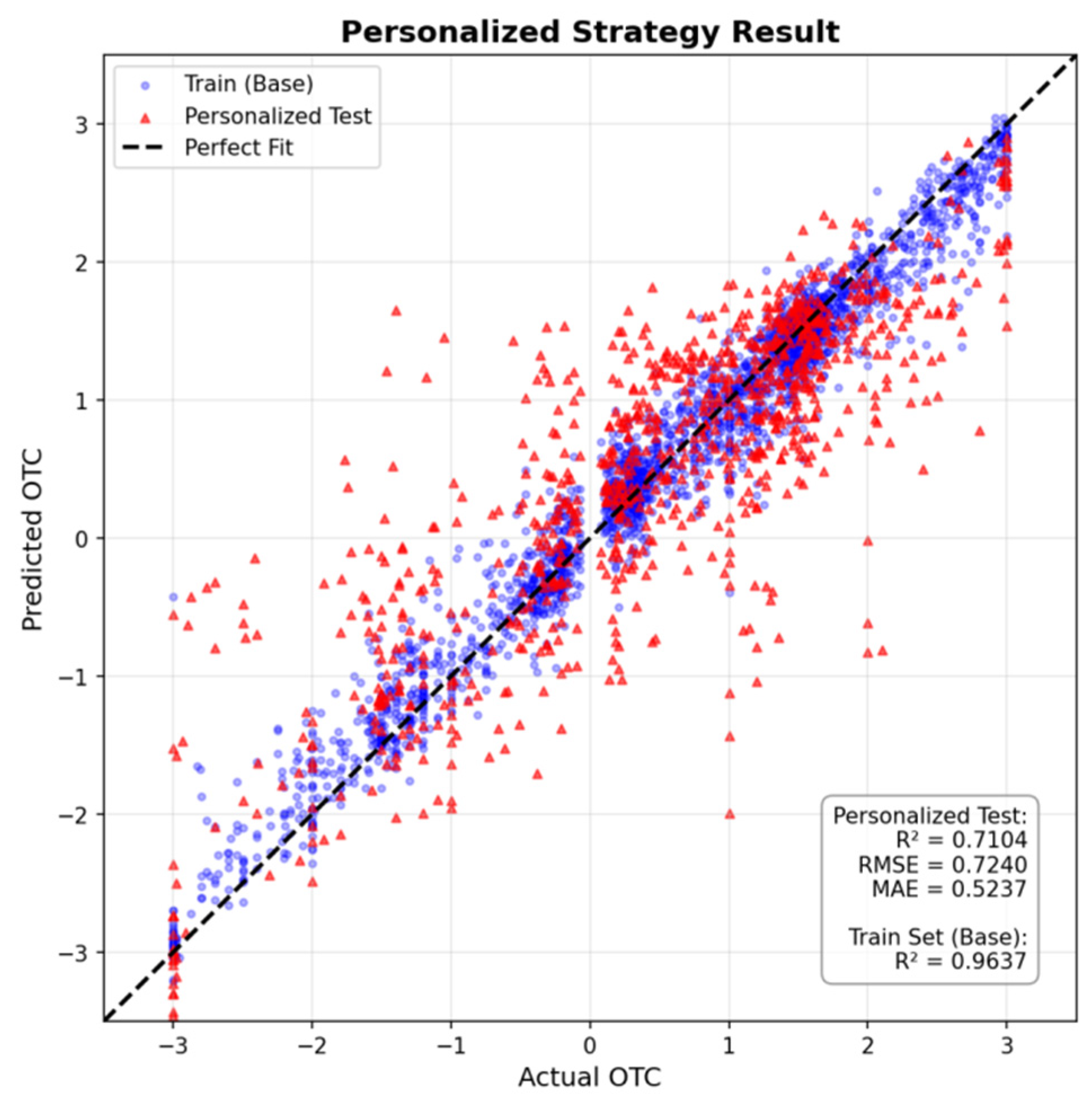
3.3.2. Selective Triggering and Few-Shot Calibration
FS-SWC does not aim to retrain the model comprehensively for every participant. Instead, it adopts an on-demand triggering mechanism: only when the system detects a substantial prediction deviation for a new user does it perform rapid calibration using a very small amount of feedback data. Specifically, during calibration, a small subset of user samples is dynamically selected (up to 8 samples) and combined with the general training set. Sample weights are adaptively adjusted according to the model’s prediction error on the user samples: larger errors receive higher weights to reinforce learning, while smaller errors receive lower weights to mitigate overfitting. This design enables fast individual adaptation with minimal interaction cost, concentrating computation on the long-tail users who truly require correction.
The results demonstrate the engineering advantages of this strategy:
- (1)
- Low trigger rate and validation of the general model’s generalizability. Among 10 test participants, only 1 participant (10%) triggered the personalized update mechanism, whereas the remaining 90% could directly use the general model with satisfactory performance. This low trigger rate indicates that the temporal features and alliesthesia-informed features constructed in this study are highly transferable across individuals, and the general model already covers the dynamic comfort patterns of most users.
- (2)
- A balance between targeted correction and global robustness. Because calibration is applied only to a small number of samples, the overall performance metrics are not artificially inflated. Nevertheless, meaningful improvements are achieved in the regions requiring correction: after personalization, the overall RMSE decreased from 0.73 to approximately 0.72, with a slight reduction in MAE, and no clear signs of overfitting were observed. This suggests that FS-SWC achieves a more appropriate balance between “local improvement” and “global stability.”
- (3)
- Long-tail correction in extreme regions. The main value of FS-SWC lies in correcting idiosyncratic preferences and errors in extreme OTC regions. The general model tends to exhibit a conservative regression-to-the-mean behavior in extremes, whereas the personalized strategy can leverage a few feedback samples to selectively adjust the model toward the user’s preference, thereby improving fit quality and user experience in these extreme regions.
Taken together, FS-SWC is not designed to uniformly boost an average metric for all users; rather, it provides a low-cost, on-demand deployment paradigm: the vast majority of users are served by the general model (≈90%), while edge-device few-shot calibration is triggered only when a small fraction of long-tail users or specific operating regions exhibit substantial deviations (≈10%). This paradigm offers a practical trade-off between computational efficiency and occupant experience, providing an engineering-feasible pathway for future HVAC systems toward “human–system co-adaptive” control strategies.
4. Discussion
4.1. Nonlinearity of Thermal Perception and Compatibility of Gradient Boosting Algorithms
The Stacking Ensemble did not outperform a single model. This likely reflects redundancy in its composition: the three base learners (HistGB, LightGBM, RandomForest) all follow a tree-splitting paradigm and thus learn similar decision boundaries on the same data, while the meta-learner (final estimator) fails to add complementary information and instead introduces noise.
Across models, tree-based gradient boosting methods (e.g., HistGB, XGBoost) consistently outperformed linear regressions (Linear, Lasso), highlighting the nonlinear nature of thermal comfort. Alliesthesia theory describes comfort as state-dependent and non-monotonic [26]: when the thermal load error is positive (Load Error > 0), a cold stimulus can be pleasant, whereas when it is negative (Load Error < 0), the same stimulus can be unpleasant. Such sign-reversal behavior cannot be captured by a single linear coefficient, but gradient boosting can represent it by partitioning the feature space into physiological regimes, consistent with the alliesthesia principle that stimulus valence depends on internal state.
Although stacking is often reported to improve accuracy [65], it still did not surpass the single HistGB model here. This suggests that after physics-informed feature engineering, different tree models (e.g., XGBoost, LightGBM) produce highly homogeneous error patterns, leaving the meta-learner little independent signal to exploit. Practically, a single strong learner tuned via Bayesian optimization may therefore be more economical than deploying a costly ensemble.
4.2. Model Performance
The prediction target of this study is dynamic overall thermal comfort (OTC). The difficulty lies not only in the time-varying nature of thermal stimuli, but also in the inherent discreteness and noise of subjective comfort votes. Therefore, model performance should not be judged as “reliable/unreliable” solely by a single R2 value; instead, it should be interpreted comprehensively in light of the rigor of the evaluation protocol, the error scale, and the error structure.
To avoid information leakage introduced by conventional random splitting, we adopted a subject-level split validation strategy: all samples from the same participant are never simultaneously included in the training and test/validation sets. This strategy effectively prevents inflated performance caused by the model “memorizing” subject-specific characteristics, making the evaluation closer to real deployment scenarios (i.e., the model must generalize to previously unseen users). Under this more challenging and more realistic setting, R2 is typically noticeably lower than that obtained with random splitting. Hence, a “not-so-high” R2 does not necessarily indicate an unreliable model; rather, it may reflect a stricter evaluation and more trustworthy results.
In addition to R2, we report error-scale metrics such as RMSE and MAE. On the 6-point scale (−3 to +3), an MAE of approximately 0.5 scale units means that the average prediction error is within about “half a scale step.” Given the unavoidable inter-individual variability and test–retest uncertainty in subjective ratings, this error magnitude is practically meaningful. In other words, even if the scatter plot appears somewhat dispersed, the model can still provide predictions with usable accuracy on the rating scale.
It should also be emphasized that our prediction target is overall thermal comfort, rather than the more commonly modeled thermal sensation. These two constructs differ in both theoretical meaning and predictability [66]. Thermal sensation mainly reflects perceived cold–hot intensity [12,15], whereas thermal comfort involves stronger subjective satisfaction and hedonic appraisal [12,19]. Its formation is influenced not only by instantaneous thermal stimuli but also by thermal history, psychological expectations, individual preferences, and adaptation processes, exhibiting more pronounced nonlinearity and state dependence. Therefore, under comparable data quality and evaluation settings, thermal comfort is typically less predictable than thermal sensation. As noted in our Introduction, many studies reporting higher predictive performance focus on thermal sensation as the target variable. In contrast, we intentionally adopt a more complex target (OTC) together with a stricter subject-level validation constraint, to strengthen the model’s generalization capability and credibility for real-world deployment to unseen users.
4.3. Feature Interpretability Analysis
The application of machine learning in the built environment is frequently criticized for lacking interpretability. This study, through SHAP value analysis, explained the model’s decision logic and validated the importance of alliesthesia theory in dynamic environments.
4.3.1. Dominance of the Temporal Dimension
SHAP analysis revealed that Time (min) is the foremost factor influencing OTC prediction (Mean |SHAP| = 0.636), with its importance surpassing even that of all environmental features. This result is consistent with physiological interpretations such as receptor adaptation [67] and temporal alliesthesia [21]. Using equipment to rapidly improve a discomfortable environment within a short period, such as activating air conditioning for cooling in a hot and stuffy environment, can trigger a brief yet intense hedonic effect, causing thermal comfort to increase rapidly [23]. Under sustained cold exposure, the discharge frequency of cutaneous cold receptors decays exponentially over time due to ion channel desensitization, causing the neural input signal serving as corrective utility to gradually diminish. Simultaneously, as the thermal load error decreases, the hedonic effect progressively fades. Throughout this entire dynamic process, a person’s environmental evaluation is determined not solely by the absolute values of environmental parameters but is also modulated by the duration of cooling [51]. However, Time may also implicitly encode broader stage/protocol information (e.g., adaptation, fatigue, or stage transitions). Therefore, we interpret Time primarily as a proxy for unobserved time-varying factors rather than an independent causal driver. The introduced alliesthesia-informed features (dynamic set point, Load Error, etc.) provide a mechanistic representation to reduce reliance on purely chronological indexing; future work can further disentangle these effects via explicit stage labeling or time-ablation analyses.
4.3.2. Setpoint Drift and Quantification of Load Error
The dynamic setpoint () and the ranked second (Mean |SHAP| = 0.208) and third (Mean |SHAP| = 0.208) in feature importance, respectively, demonstrating the effectiveness of introducing AIML operators. The model did not simply predict based on absolute skin temperature (tsk) but rather based on the relative deviation between tsk and (i.e., the ).
4.3.3. Thermal Inertia Effect of Body Morphology
The high ranking of BMI (Mean |SHAP| = 0.098) and body surface area (Mean |SHAP| = 0.090) in the SHAP analysis reveals the modulatory role of whole-body thermal inertia in comfort perception. But it should be noted that the BMI range in our sample was relatively narrow, which may limit the statistical power to isolate its independent effect. The observed SHAP importance of BMI might partially stem from its correlation with body surface area and weight. Future studies with a wider BMI distribution are needed to confirm these findings.
4.4. Personalized Calibration Strategy: A Practical Pathway for Addressing Long-Tail Distributions
The general model faced challenges when dealing with “thermal outliers.” The few-shot selective weighting calibration (FS-SWC) strategy proposed in this study demonstrated an efficient solution. Experimental results showed that fine-tuning with only the first 20% of a new user’s data can significantly correct extreme deviations. More interestingly, only 10% of users triggered the personalization mechanism, while 90% could directly use the general model. This reveals the bimodal distribution characteristic of thermal comfort perception:
The physiological majority: The vast majority of individuals’ alliesthesia mechanisms follow similar biophysical principles (e.g., response to Load Error), and the general AIML model provides sufficient coverage.
The specific minority: A small number of individuals exhibit responses that significantly deviate from the population due to exceptional metabolic rates, clothing habits, or psychological preferences.
The value of the FS-SWC strategy lies in its on-demand computing characteristic: the system does not require expensive retraining for all users but merely identifies and performs few-shot learning on the 10% of “idiosyncratic users.” This resolves the “cold start” problem common in intelligent buildings—that is, when new users have no data, the general model can be used first, progressively evolving into a personalized model as data accumulate.
4.5. Limitations and Future Perspectives
Although this study has made progress in theoretical integration and algorithmic performance, limitations remain on the path toward practical engineering applications.
First, it should be noted that the BMI range in our sample was relatively narrow, which may limit the statistical power to isolate its independent effect. The observed SHAP importance of BMI might partially stem from its correlation with body surface area (ADu) and weight. Future studies with a wider BMI distribution are needed to confirm these findings. Second, the current model relies on contact-based skin temperature sensors (thermocouples/thermistors), which are difficult to deploy in practical office environments. Future research should focus on developing virtual sensing technologies utilizing infrared thermography or estimating skin temperature through low-cost environmental sensors combined with human body heat balance equations. Third, the dataset of this study was primarily collected under summer cooling conditions. Seasonal alliesthesia research suggests that the human thermal setpoint exhibits significant seasonal drift [12]. The current model may require additional data from other seasons or the introduction of seasonal correction factors to accommodate cross-seasonal operational requirements. Fourth, the environmental indicators considered in this study are limited. Future work may incorporate additional environmental indicators (e.g., ventilation performance characterization) to further improve the interpretability of the conclusions and the model’s predictive performance. Fifth, this study is limited to intermittent split-unit cooling with two temperature settings (23 °C and 26 °C) in residential environments. The findings may not directly apply to other HVAC systems, such as centralized or radiant systems. Future work will be needed to validate the model in broader HVAC contexts and under different conditions. Sixth, the accuracy of the instruments used in this study (particularly the temperature meter, the humidity meter, and the thermocouples) is lower than the values recommended by the international standards ISO 7726 [68] and ISO 9886 [69]. This measurement uncertainty [70] may, to some extent, limit the attainable upper bound of the model’s performance. In future work, we will seek to use higher-accuracy instruments to obtain more accurate objective parameters, thereby further improving the model’s predictive performance. Finally, according to Cabanac’s research findings [71], alliesthesia is not limited to thermal sensation. Visual stimuli (warm/cool color temperature lighting) [72] and auditory environments [73] may influence comfort through cross-modal perception. Future AIML frameworks should explore the incorporation of multi-physics features to construct more comprehensive indoor environmental quality prediction models.
In summary, this study demonstrates that translating alliesthesia theory into computable machine learning features can enhance the accuracy and interpretability of thermal comfort prediction. We call for a paradigm shift in built environment control from “maintaining constant temperature” to “managing dynamic hedonic pleasure”.
5. Conclusions
Addressing the challenge of dynamic thermal comfort prediction in non-steady-state thermal environments, this study proposed and validated an alliesthesia-informed machine learning (AIML) framework. By translating alliesthesia theory into computable mathematical features, a feature operator set incorporating dynamic setpoint, load errors, and s was constructed, and the performance of 13 machine learning models in overall thermal comfort (OTC) prediction was evaluated. The main conclusions are as follows:
- (1)
- This study showed that the explicit introduction of alliesthesia theory-guided feature engineering can effectively capture the nonlinearity, state-dependency, and temporal dynamics inherent in thermal comfort perception. The AIML model based on Histogram-based Gradient Boosting (HistGB) achieved excellent performance on the independent test set with R2 = 0.71, RMSE = 0.73, and MAE = 0.53.
- (2)
- SHAP interpretability analysis revealed that exposure time and alliesthesia operators occupy dominant positions in feature importance rankings, with their contributions far exceeding those of conventional environmental parameters.
- (3)
- Compared to linear models, gradient boosting algorithms (e.g., HistGB, XGBoost) can naturally partition the feature space through tree structures, characterizing the non-monotonic property of “stimulus valence reversal contingent on internal state” described in alliesthesia theory, thereby providing superior compatibility with dynamic thermal comfort prediction tasks.
- (4)
- The proposed few-shot selective weighting calibration (FS-SWC) strategy requires only the first 20% of a user’s data for model fine-tuning. In practical testing, 10% of participants triggered personalized calibration, while the vast majority of users could directly use the general AIML model, reflecting the model’s robust cross-population generalizability and engineering practicality.
- (5)
- This study advances a paradigm shift in thermal comfort modeling from “static thermal neutrality” to “dynamic thermal hedonics,” providing theoretical foundations and algorithmic support for HVAC systems to achieve “on-demand comfort” control strategies that balance energy efficiency with occupant experience. Through interpretable feature design and personalized adaptation mechanisms, the AIML framework enhances model credibility and deployability in real-world scenarios while maintaining high accuracy.
Author Contributions
T.W.: Writing—review and editing, Supervision. W.H.: Writing—original draft, Writing—review and editing, Methodology, Visualization, Conceptualization. H.Y.: Writing—review and editing, Resources, Supervision, Conceptualization, Project administration. S.Z.: Writing—review and editing, Methodology, Visualization, Conceptualization. R.S.: Writing—review and editing. Y.G.: Writing—review and editing. Y.L.: Writing—review and editing. All authors have read and agreed to the published version of the manuscript.
Funding
This research was supported by the National Natural Science Foundation of China (Grant No. 52378095), the Key Research Project Support Program for Higher Education Institutions in Henan Province (Grant No. 24A410001 and 26A410002), the International Science and Technology Cooperation Program of Henan Province (Grant No. 252102521004), and the Natural Science Foundation of Henan (Grant No. 252300423404).
Institutional Review Board Statement
The study was conducted in accordance with the Declaration of Helsinki, and the protocol was approved by the Local Ethics Committee of Henan Polytechnic University (Project identification code: HPULLSC2025-003) on 28 February 2025.
Informed Consent Statement
Written informed consent was obtained from all subjects involved in the study.
Data Availability Statement
This research includes data currently under review, as part of a broader project. We will share information with those interested by contacting correspondence authors through the following emails: yhy@hpu.edu.cn.
Acknowledgments
During the preparation of this manuscript, the authors used Gemini 3.0 for the purposes of partial language polishing and information proofreading. The authors have reviewed and edited the output and take full responsibility for the content of this publication.
Conflicts of Interest
The authors declare no conflicts of interest.
Appendix A
For the symbols appearing in the text, Appendix A provides a summary of relevant information. The important symbols, abbreviations, and their units used in this manuscript are shown in the Table A1.
Table A1.
Symbols, abbreviations, and units.
References
- Zhou, X.; Lian, Z.; Li, L. An individualized human thermoregulation model for Chinese adults. Build. Environ. 2013, 70, 257–265. [Google Scholar] [CrossRef] [Scilit]
- Yan, H.; Guo, Y.; Zhang, H.; Schiavon, S.; Sun, R.; Zhao, S.; Sun, Z.; Shi, F. Effects of intermittent cooling on human thermophysiological and perceptual responses in a non-steady-state thermal environment. Build. Environ. 2025, 287, 113751. [Google Scholar] [CrossRef] [Scilit]
- He, Y.; Parkinson, T.; Arens, E.; Zhang, H.; Li, N.; Peng, J.; Elson, J.; Maranville, C. Creating alliesthesia in cool environments using personal comfort systems. Build. Environ. 2022, 209, 108642. [Google Scholar] [CrossRef] [Scilit]
- Fanger, P. Thermal Comfort: Analysis and Applications in Environmental Engineering; Danish Technical Press: Copenhagen, Denmark, 1970; Available online: https://archive.org/details/thermalcomfortan0000fang/page/248/mode/2up (accessed on 7 March 2026).
- de Dear, R.; Brager, G.S. Developing an adaptive model of thermal comfort and preference. ASHRAE Trans. 1998, 104, 1. [Google Scholar]
- Broday, E.E.; Moreto, J.A.; Xavier, A.A.d.P.; de Oliveira, R. The approximation between thermal sensation votes (OTS) and predicted mean vote (PMV): A comparative analysis. Int. J. Ind. Ergon. 2019, 69, 1–8. [Google Scholar] [CrossRef] [Scilit]
- de Dear, R.J.; Brager, G.S. Thermal comfort in naturally ventilated buildings: Revisions to ASHRAE standard 55. Energy Build. 2002, 34, 549–561. [Google Scholar] [CrossRef] [Scilit]
- Vargas, G.A.; Stevenson, F. Thermal memory and transition in lobby spaces. Energy Procedia 2014, 62, 502–511. [Google Scholar] [CrossRef] [Scilit]
- Ganesh, G.A.; Sinha, S.L.; Verma, T.N.; Dewangan, S.K. Investigation of indoor environment quality and factors affecting human comfort: A critical review. Build. Environ. 2021, 204, 108146. [Google Scholar] [CrossRef] [Scilit]
- Wu, Z.; Wagner, A. Effect of short-term thermal history on thermal comfort and physiological responses: A pilot study. Energy Build. 2023, 298, 113510. [Google Scholar] [CrossRef] [Scilit]
- Cândido, C.; de Dear, R.; Lamberts, R.; Bittencourt, L. Cooling exposure in hot humid climates: Are occupants “addicted”? Archit. Sci. Rev. 2010, 53, 59–64. [Google Scholar] [CrossRef] [Scilit]
- Schweiker, M.; Schakib-Ekbatan, K.; Fuchs, X.; Becker, S. A seasonal approach to alliesthesia. Is there a conflict with thermal adaptation? Energy Build. 2020, 212, 109745. [Google Scholar] [CrossRef] [Scilit]
- Pourghorban, A.; Chang, V.W.; Zhou, J. Electroencephalograph (EEG) Insights into Short-Term Thermal Adaptation and Alliesthesia: From Rapid Change to Steady State. Build. Environ. 2025, 280, 113098. [Google Scholar] [CrossRef] [Scilit]
- Cabanac, M. Physiological role of pleasure: A stimulus can feel pleasant or unpleasant depending upon its usefulness as determined by internal signals. Science 1971, 173, 1103–1107. [Google Scholar] [CrossRef] [Scilit] [PubMed]
- Zhao, Q.; Lyu, J.; Du, H.; Lian, Z.; Zhao, Z. Gender differences in thermal sensation and skin temperature sensitivity under local cooling. J. Therm. Biol. 2023, 111, 103401. [Google Scholar] [CrossRef] [Scilit]
- Luo, M.; Wang, Z.; Zhang, H.; Arens, E.; Filingeri, D.; Jin, L.; Ghahramani, A.; Chen, W.; He, Y.; Si, B. High-density thermal sensitivity maps of the human body. Build. Environ. 2020, 167, 106435. [Google Scholar] [CrossRef] [Scilit]
- Meimand, M.; Jazizadeh, F. A personal touch to demand response: An occupant-centric control strategy for HVAC systems using personalized comfort models. Energy Build. 2024, 303, 113769. [Google Scholar] [CrossRef] [Scilit]
- Barone, G.; Buonomano, A.; Forzano, C.; Giuzio, G.; Palombo, A.; Russo, G. A new thermal comfort model based on physiological parameters for the smart design and control of energy-efficient HVAC systems. Renew. Sustain. Energy Rev. 2023, 173, 113015. [Google Scholar] [CrossRef] [Scilit]
- Wang, Z.; Wang, J.; He, Y.; Liu, Y.; Lin, B.; Hong, T. Dimension analysis of subjective thermal comfort metrics based on ASHRAE Global Thermal Comfort Database using machine learning. J. Build. Eng. 2020, 29, 101120. [Google Scholar] [CrossRef] [Scilit]
- Parkinson, T.; de Dear, R.; Candido, C. Thermal pleasure in built environments: Alliesthesia in different thermoregulatory zones. Build. Res. Inf. 2016, 44, 20–33. [Google Scholar] [CrossRef] [Scilit]
- Liu, S.; Nazarian, N.; Hart, M.A.; Niu, J.; Xie, Y.; de Dear, R. Dynamic thermal pleasure in outdoor environments-temporal alliesthesia. Sci. Total Environ. 2021, 771, 144910. [Google Scholar] [CrossRef] [Scilit]
- Arens, E.; Zhang, H.; Huizenga, C. Partial- and whole-body thermal sensation and comfort—Part II: Non-uniform environmental conditions. J. Therm. Biol. 2006, 31, 60–66. [Google Scholar] [CrossRef] [Scilit]
- Jiang, Y.; Xie, Y.; Niu, J. Short-term dynamic thermal perception and physiological response to step changes between real-life indoor and outdoor environments. Build. Environ. 2024, 251, 111223. [Google Scholar] [CrossRef] [Scilit]
- Parkinson, T.; de Dear, R.J. Thermal pleasure in built environments: Physiology of alliesthesia. Build. Res. Inf. 2014, 43, 288–301. [Google Scholar] [CrossRef] [Scilit]
- Parkinson, T.; de Dear, R.J. Thermal pleasure in built environments: Spatial alliesthesia from contact heating. Build. Res. Inf. 2015, 44, 248–262. [Google Scholar] [CrossRef] [Scilit]
- Parkinson, T.; de Dear, R.J. Thermal pleasure in built environments: Spatial alliesthesia from air movement. Build. Res. Inf. 2016, 45, 320–335. [Google Scholar] [CrossRef] [Scilit]
- Farhan, A.A.; Pattipati, K.; Wang, B.; Luh, P. Predicting individual thermal comfort using machine learning algorithms. In Proceedings of the IEEE International Conference on Automation Science and Engineering, Gothenburg, Sweden, 24–28 August 2015; pp. 708–713. [Google Scholar] [CrossRef] [Scilit]
- Lu, S.; Wang, W.; Lin, C.; Hameen, E.C. Data-driven simulation of a thermal comfort-based temperature set-point control with ASHRAE RP884. Build. Environ. 2019, 156, 137–146. [Google Scholar] [CrossRef] [Scilit]
- Luo, M.; Xie, J.; Yan, Y.; Ke, Z.; Yu, P.; Wang, Z.; Zhang, J. Comparing machine learning algorithms in predicting thermal sensation using ASHRAE Comfort Database II. Energy Build. 2020, 210, 109776. [Google Scholar] [CrossRef] [Scilit]
- Zhou, X.; Xu, L.; Zhang, J.; Niu, B.; Luo, M.; Zhou, G.; Zhang, X. Data-driven thermal comfort model via support vector machine algorithms: Insights from ASHRAE RP-884 database. Energy Build. 2020, 211, 109795. [Google Scholar] [CrossRef] [Scilit]
- Ma, N.; Chen, L.; Hu, J.; Perdikaris, P.; Braham, W.W. Adaptive behavior and different thermal experiences of real people: A Bayesian neural network approach to thermal preference prediction and classification. Build. Environ. 2021, 198, 107875. [Google Scholar] [CrossRef] [Scilit]
- Lala, B.; Rizk, H.; Kala, S.M.; Hagishima, A. Multi-task learning for concurrent prediction of thermal comfort, sensation and preference in winters. Buildings 2022, 12, 750. [Google Scholar] [CrossRef] [Scilit]
- Baek, J.; Park, D.Y.; Park, H.; Le, D.M.; Chang, S. Vision-based personal thermal comfort prediction based on half-body thermal distribution. Build. Environ. 2023, 228, 109877. [Google Scholar] [CrossRef] [Scilit]
- Lan, H.; Hou, H.C.; Gou, Z. A machine learning led investigation to understand individual difference and the human-environment interactive effect on classroom thermal comfort. Build. Environ. 2023, 236, 110259. [Google Scholar] [CrossRef] [Scilit]
- Guo, R.; Yang, B.; Guo, Y.; Li, H.; Li, Z.; Zhou, B.; Hong, B.; Wang, F. Machine learning-based prediction of outdoor thermal comfort: Combining Bayesian optimization and the SHAP model. Build. Environ. 2024, 254, 111301. [Google Scholar] [CrossRef] [Scilit]
- Rudin, C. Stop explaining black box machine learning models for high stakes decisions and use interpretable models instead. Nat. Mach. Intell. 2019, 1, 206–215. [Google Scholar] [CrossRef] [Scilit]
- de Dear, R.J. Global database of thermal comfort field experiments. ASHRAE Trans. 1998, 104, 1141–1152. [Google Scholar]
- de Dear, R.J.; Brager, G.S.; Cooper, D. Developing an adaptive model of thermal comfort and preference—Final report on RP-884. ASHRAE Trans. 1997, 104, 291. [Google Scholar]
- Yang, B.; Li, X.; Liu, Y.; Chen, L.; Guo, R.; Wang, F.; Yan, K.; Yan, K. Comparison of models for predicting winter individual thermal comfort based on machine learning algorithms. Build. Environ. 2022, 215, 108970. [Google Scholar] [CrossRef] [Scilit]
- Park, J.; Choi, H.; Kim, D.; Kim, T. Development of novel PMV-based HVAC control strategies using a mean radiant temperature prediction model by machine learning in Kuwaiti climate. Build. Environ. 2021, 206, 108357. [Google Scholar] [CrossRef] [Scilit]
- Alfano, F.R.D.; Olesen, B.W.; Palella, B.I.; Riccio, G. Thermal comfort: Design and assessment for energy saving. Energy Build. 2014, 81, 326–336. [Google Scholar] [CrossRef] [Scilit]
- ASHRAE ANSI/ASHRAE Standard 55-2023; Thermal Environmental Conditions for Human Occupancy. American Society of Heating, Refrigerating and Air-Conditioning Engineers: Atlanta, GA, USA, 2023.
- ISO Standard 7730; Ergonomics of the Thermal Environment—Analytical Determination and Interpretation of Thermal Comfort Using Calculation of the PMV and PPD Indices and Local Thermal Comfort Criteria. ISO: Geneva, Switzerland, 2025.
- Zhou, J.; Zhang, X.; Xie, J.; Liu, J. Effects of elevated air speed on thermal comfort in hot-humid climate and the extended summer comfort zone. Energy Build. 2023, 287, 112953. [Google Scholar] [CrossRef] [Scilit]
- Luo, M.; Ji, W.; Cao, B.; Ouyang, Q.; Zhu, Y. Indoor climate and thermal physiological adaptation: Evidences from migrants with different cold indoor exposures. Build. Environ. 2016, 98, 30–38. [Google Scholar] [CrossRef] [Scilit]
- Schweiker, M.; Andersen, R.K.; Carlucci, S.; Chinazzo, G.; Hodder, S.; Mahdavi, A.; Palella, B.I.; Pisello, A.L.; Alfano, F.R.D.; Vellei, M. Ten questions concerning the usage of subjective assessment scales in research on indoor environmental quality. Build. Environ. 2025, 283, 113393. [Google Scholar] [CrossRef] [Scilit]
- Wu, Y.; Zhang, Z.; Liu, H.; Li, B.; Kosonen, R.; Jokisalo, J.; Wang, W. Effect of change rates and directions of air temperature ramps on thermal responses of occupants under warm summer conditions. Build. Environ. 2023, 243, 110614. [Google Scholar] [CrossRef] [Scilit]
- Gagge, A.P.; Fobelets, A.P.; Berglund, L.G. A standard predictive index of human response to the thermal environment. Build. Eng. 1986, 92, 709–731. [Google Scholar]
- Cabanac, M. Adjustable set point: To honor Harold, T. Hammel. J. Appl. Physiol. 2006, 100, 1338–1346. [Google Scholar] [CrossRef] [Scilit]
- Zhang, H.; Arens, E.; Huizenga, C.; Han, T. Thermal sensation and comfort models for non-uniform and transient environments, part III: Whole-body sensation and comfort. Build. Environ. 2010, 45, 399–410. [Google Scholar] [CrossRef] [Scilit]
- Jian, Y.; Hou, Y.; Liu, W.; Chang, X. How the coldest local thermal sensation affects overall thermal sensation after turning on the air conditioning—Evidence from chamber experiments. Build. Environ. 2021, 191, 107589. [Google Scholar] [CrossRef] [Scilit]
- Yan, H.; Gao, J.; Zhao, W.; Liu, C.; Li, S.; Li, Y. Evaluation of Seasonal Variations of Human Subjective Responses in China’s Cold Climate Zone. Indoor Air 2024, 7877266. [Google Scholar] [CrossRef] [Scilit]
- Takefuji, Y. Beyond XGBoost and SHAP: Unveiling true feature importance. J. Hazard. Mater. 2025, 488, 137382. [Google Scholar] [CrossRef] [Scilit] [PubMed]
- Sevgen, E.; Abdikan, S. Classification of large-scale mobile laser scanning data in urban area with LightGBM. Remote Sens. 2023, 15, 3787. [Google Scholar] [CrossRef] [Scilit]
- Luo, M.; Wang, Y.; Xie, Y.; Zhou, L.; Qiao, J.; Qiu, S.; Sun, Y. Combination of feature selection and catboost for prediction: The first application to the estimation of aboveground biomass. Forests 2021, 12, 216. [Google Scholar] [CrossRef] [Scilit]
- Zhang, H.; Zhang, Z.; Nie, X.; Zhang, C.; Lv, H.; Yan, W. A New Method of Identification of Water-Flooded Layers Based on HistGBDT Algorithm—A Case of the Penglai 19-3 Oilfield. Processes 2025, 13, 3219. [Google Scholar] [CrossRef] [Scilit]
- Suarez-Fernandez, G.E.; Martinez-Sanchez, J.; Arias, P. Enhancing carbon stock estimation in forests: Integrating multi-data predictors with random forest method. Ecol. Inform. 2025, 86, 102997. [Google Scholar] [CrossRef] [Scilit]
- Vichai, K.; Tran, D.T.; Shiau, J.; Keawsawasvong, S.; Jamsawang, P. Predicting failure envelopes of skirted spudcan footings under combined loads using ACO optimized extremely randomized trees. Mar. Struct. 2025, 104, 103890. [Google Scholar] [CrossRef] [Scilit]
- Wang, Y.; Yan, X.; Huo, R.; Zhao, L.; Peng, J.; Hong, Y.; Liu, J. Predicting soil organic matter using corrected field spectra and stacking ensemble learning. Geoderma 2025, 460, 117417. [Google Scholar] [CrossRef] [Scilit]
- Roy, A.; Chakraborty, S. Support vector machine in structural reliability analysis: A review. Reliab. Eng. Syst. Saf. 2023, 233, 109126. [Google Scholar] [CrossRef] [Scilit]
- Xie, J.; Xiang, X.; Xia, S.; Jiang, L.; Wang, G.; Gao, X. Mgnr: A multi-granularity neighbor relationship and its application in knn classification and clustering methods. IEEE Trans. Pattern Anal. Mach. Intell. 2024, 46, 7956–7972. [Google Scholar] [CrossRef] [Scilit] [PubMed]
- Wang, X.; Wang, X.; Ma, B.; Li, Q.; Wang, C.; Shi, Y. High-performance reversible data hiding based on ridge regression prediction algorithm. Signal Process. 2023, 204, 108818. [Google Scholar] [CrossRef] [Scilit]
- Ouyang, X.; Ran, X.; Xu, H.; Al-Abssi, R.; Zhao, Y.-L.; Link, A.J.; Yang, Z.J. LassoPred: A tool to predict the 3D structure of lasso peptides. Nat. Commun. 2025, 16, 5497. [Google Scholar] [CrossRef] [Scilit]
- Zou, W.; Yao, X.; Chen, Y.; Li, X.; Huang, J.; Zhang, Y.; Yu, L.; Xie, B. An elastic net regression model for predicting the risk of ICU admission and death for hospitalized patients with COVID-19. Sci. Rep. 2024, 14, 14404. [Google Scholar] [CrossRef] [Scilit]
- Song, W.; Yu, S.; Liu, Z.; Tang, R.; Ding, Q.; Zhou, S.; Wang, X. Predicting thermal comfort of healthcare workers in hot environments based on machine learning algorithms. Energy Build. 2025, 347, 116409. [Google Scholar] [CrossRef] [Scilit]
- Vellei, M.; de Dear, R.; Inard, C.; Jay, O. Dynamic thermal perception: A review and agenda for future experimental research. Build. Environ. 2021, 205, 108269. [Google Scholar] [CrossRef] [Scilit]
- McKemy, D.D.; Neuhausser, W.M.; Julius, D. Identification of a cold receptor reveals a general role for TRP channels in thermosensation. Nature 2002, 416, 52–58. [Google Scholar] [CrossRef] [Scilit] [PubMed]
- ISO7726:2025; Ergonomics of the Thermal Environment—Instruments for Measuring Physical Quantities. International Standardization Organization: Geneva, Switzerland, 2025.
- ISO 9886:2004; Ergonomics—Evaluation of Thermal Strain by Physiological Measurements. 2nd ed. International Organization for Standardization: Geneva, Switzerland, 2004.
- Dell’iSola, M.; Frattolillo, A.; Palella, B.I.; Riccio, G. Influence of measurement uncertainties on the thermal environment assessment. Int. J. Thermophys. 2012, 33, 1616–1632. [Google Scholar] [CrossRef] [Scilit]
- Cabanac, M.; Brondel, L.; Cabanac, A. Alliesthesia. Up-date of the word and concept. Am. J. Biomed. Sci. Res. 2020, 8, 313–320. [Google Scholar] [CrossRef] [Scilit]
- Luo, W.; Kramer, R.; Kompier, M.; Smolders, K.; de Kort, Y.; Lichtenbelt, W.V.M. Effects of correlated color temperature of light on thermal comfort, thermophysiology and cognitive performance. Build. Environ. 2023, 231, 109944. [Google Scholar] [CrossRef] [Scilit]
- Sandage, M.J.; Rahn, K.A.; Smith, A.G. Vocal ergonomics in the workplace: Heating, ventilation, and air-conditioning method influences on vocal comfort and function. J. Speech Lang. Hear. Res. 2017, 60, 355–363. [Google Scholar] [CrossRef] [Scilit]
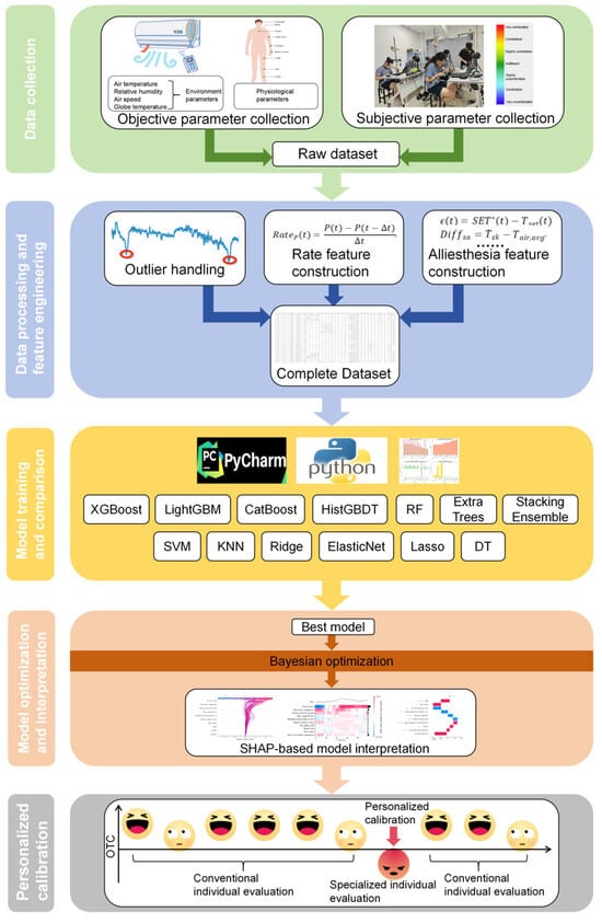
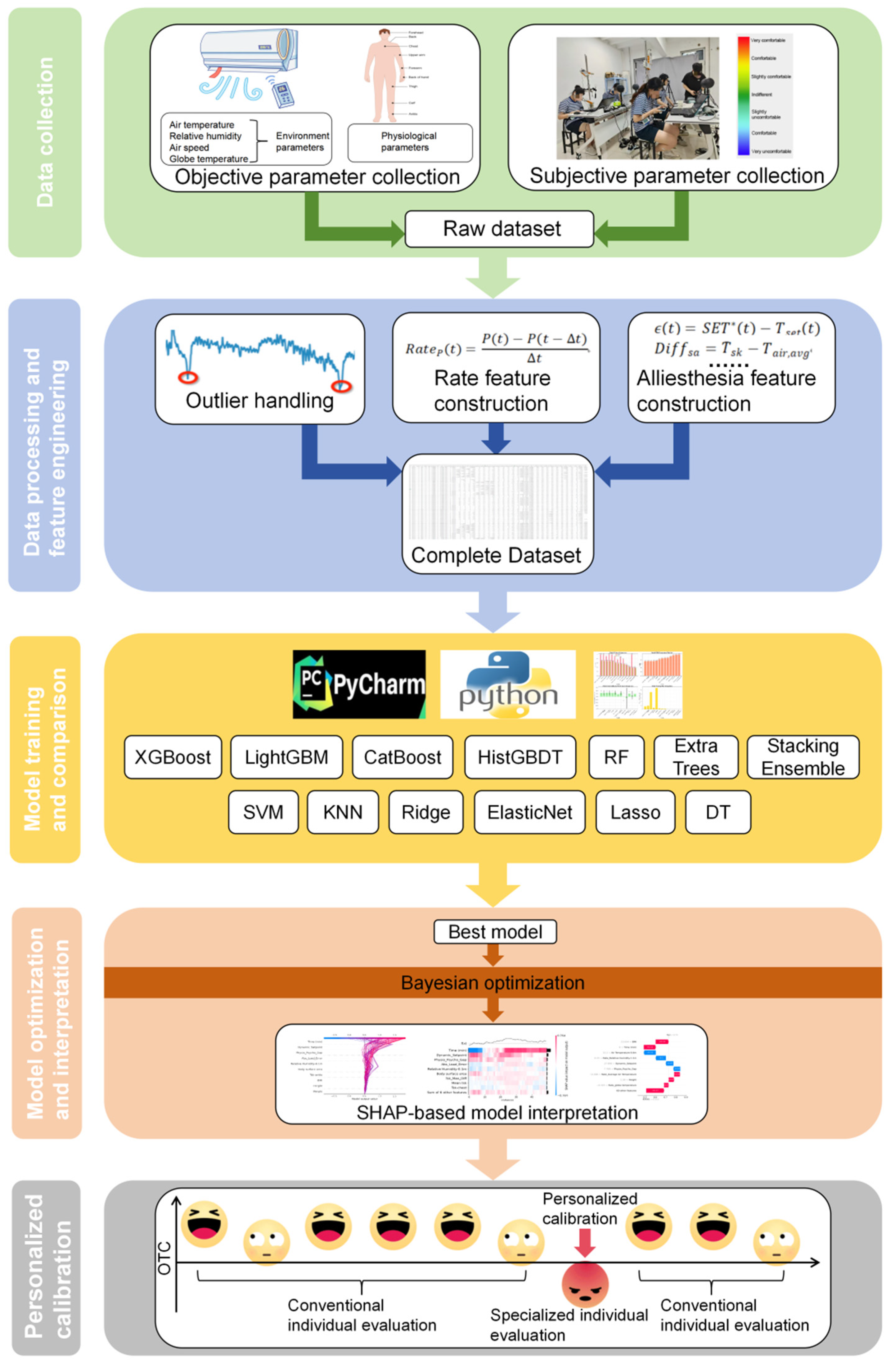
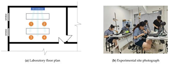
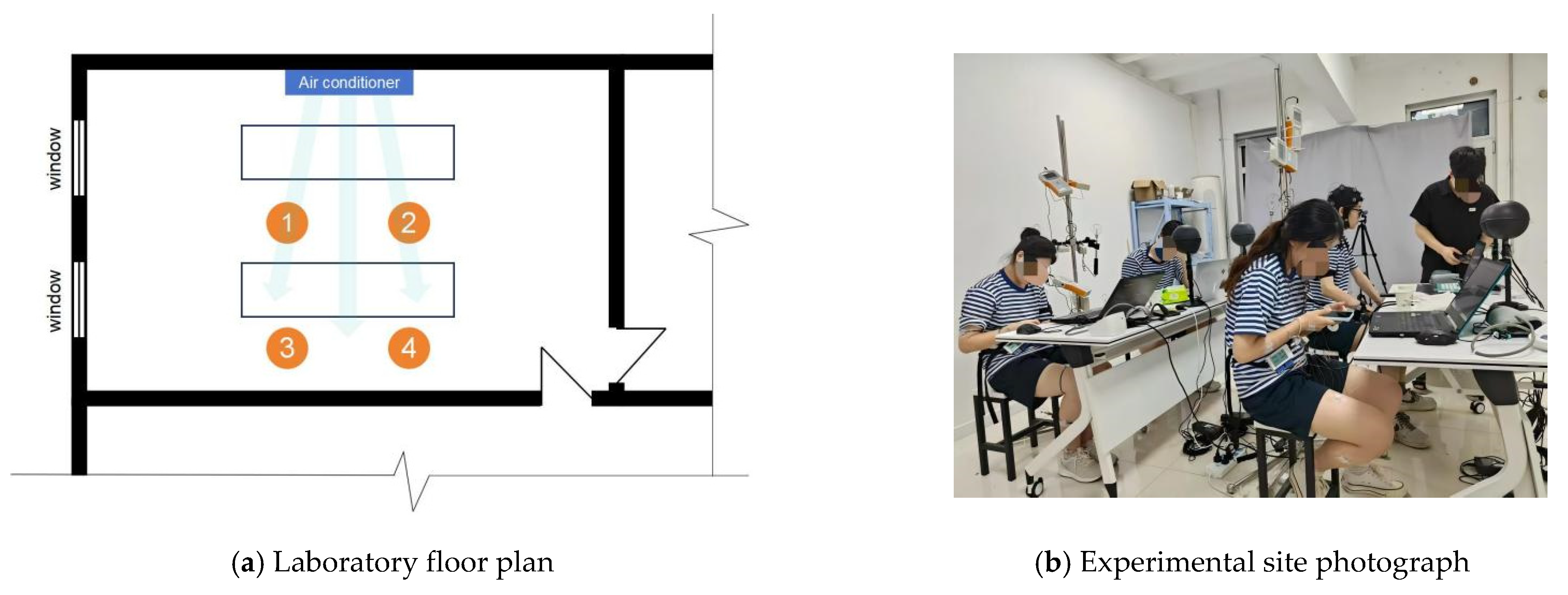
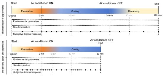
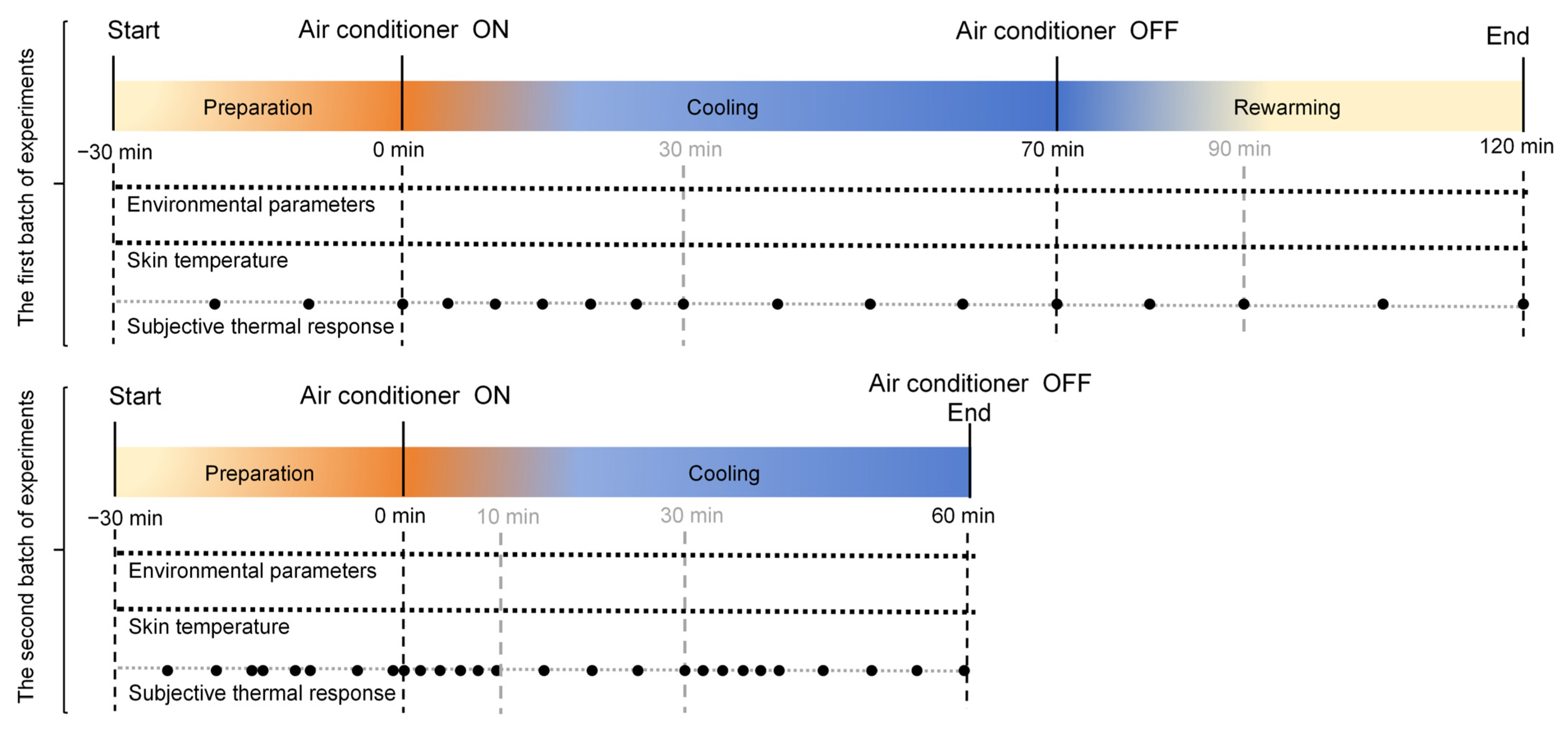
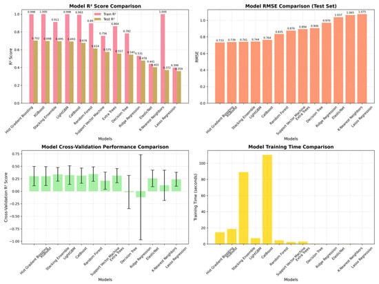
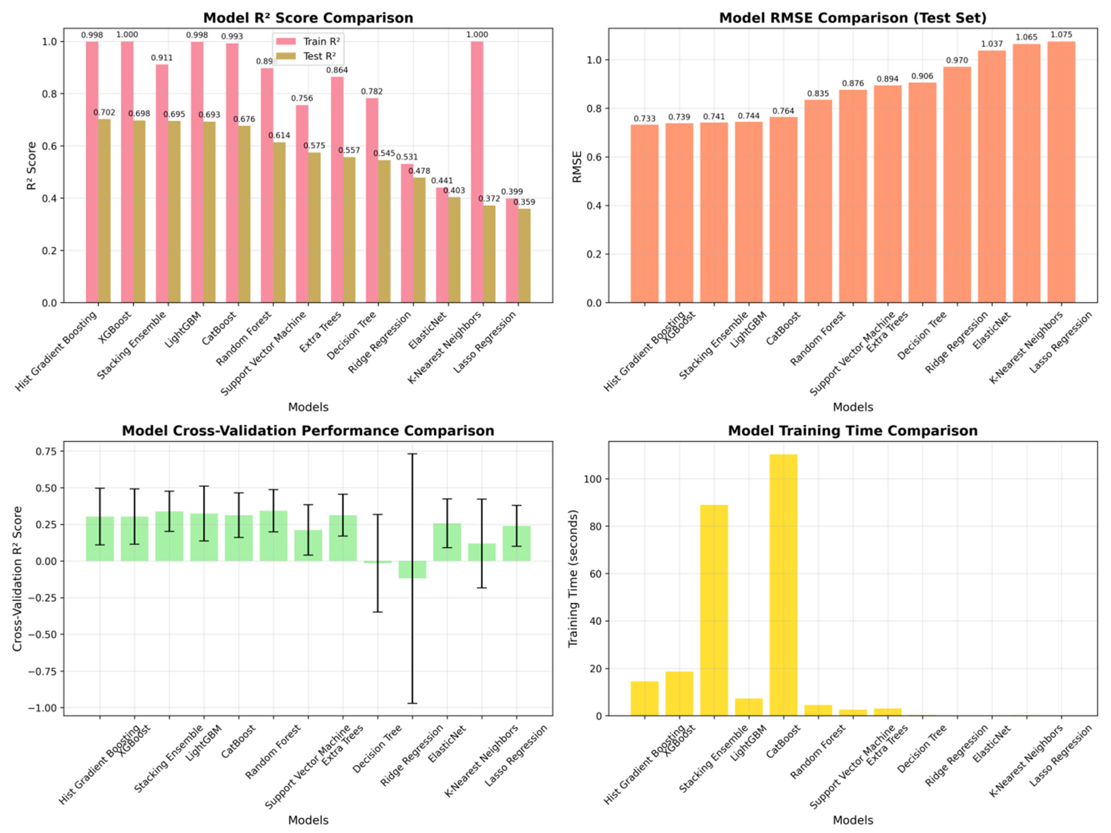
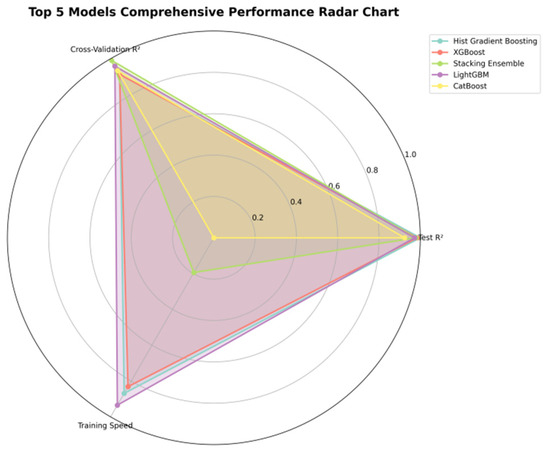
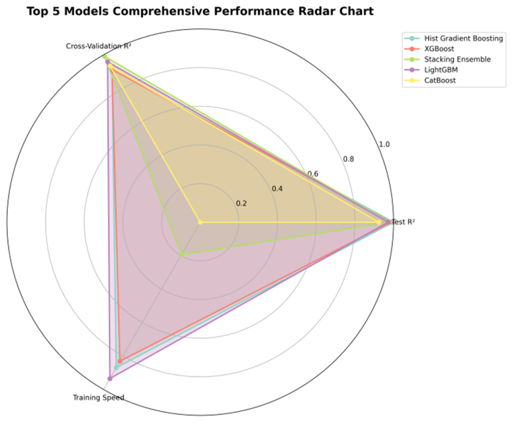
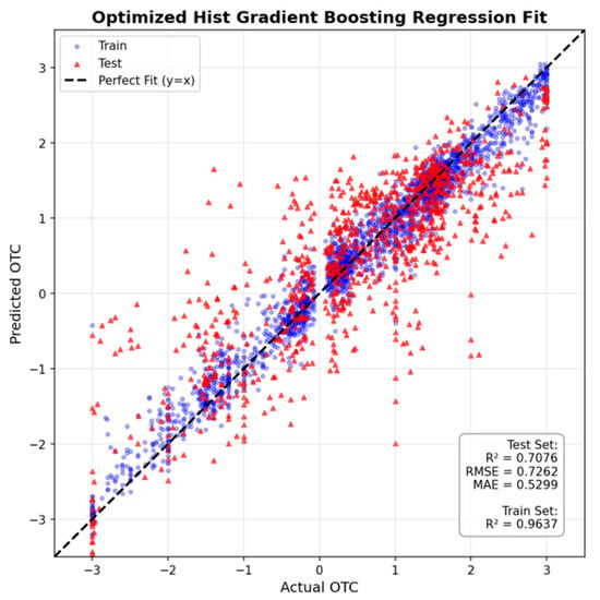
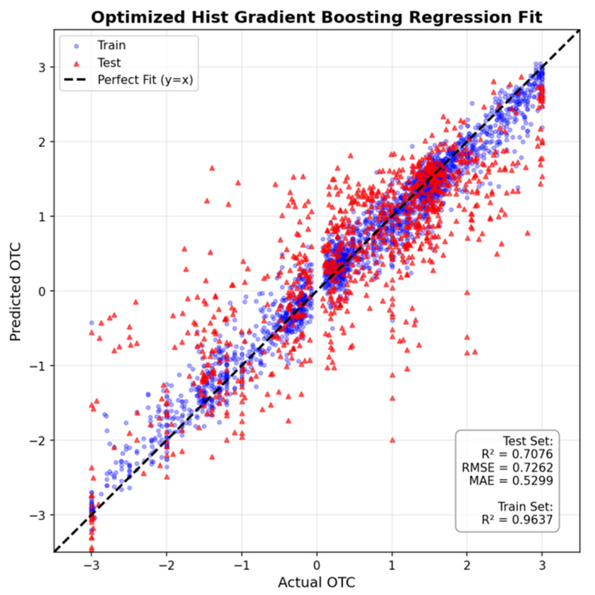
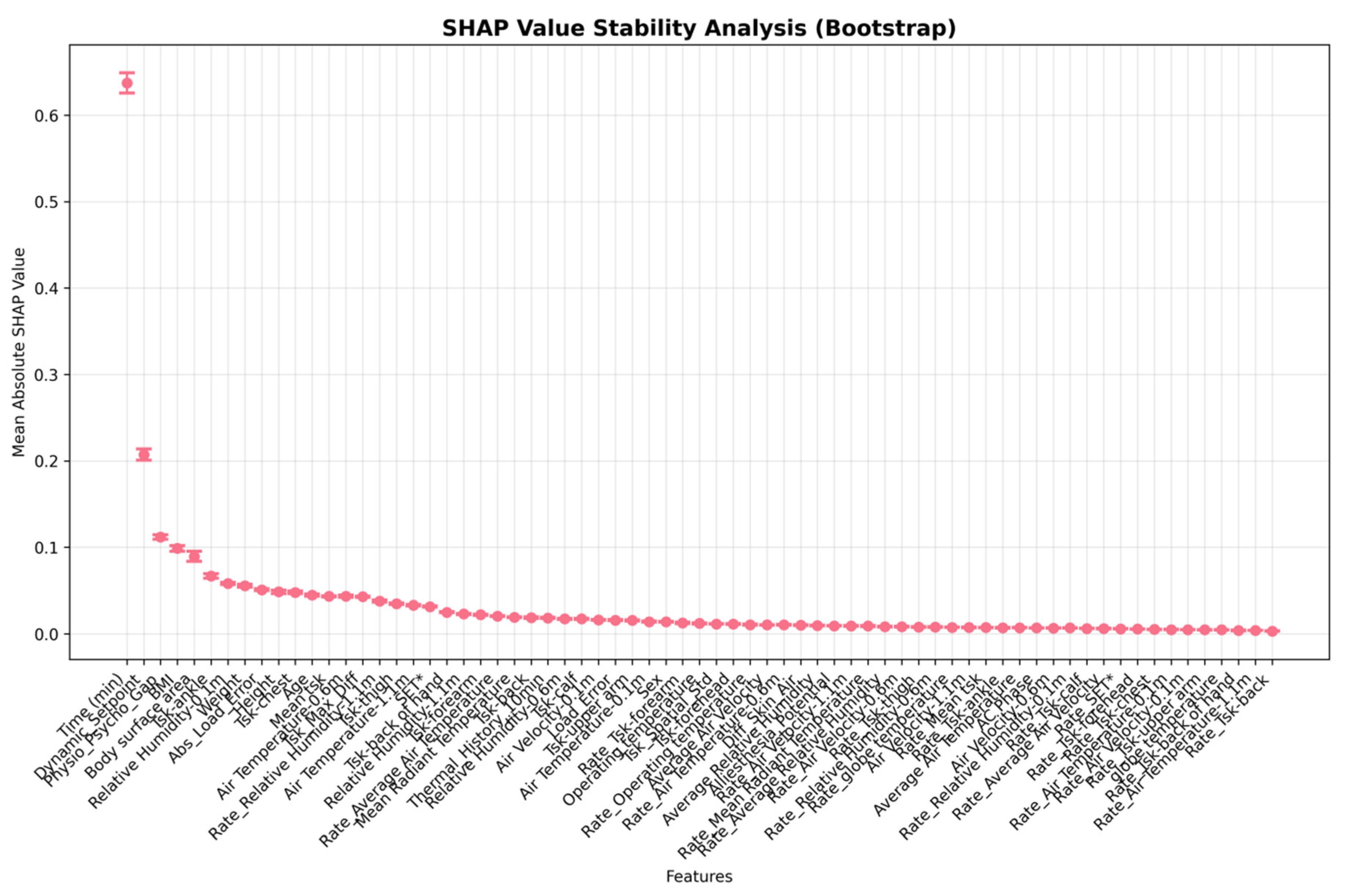
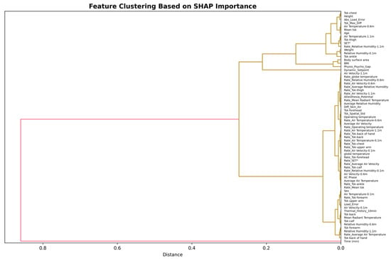
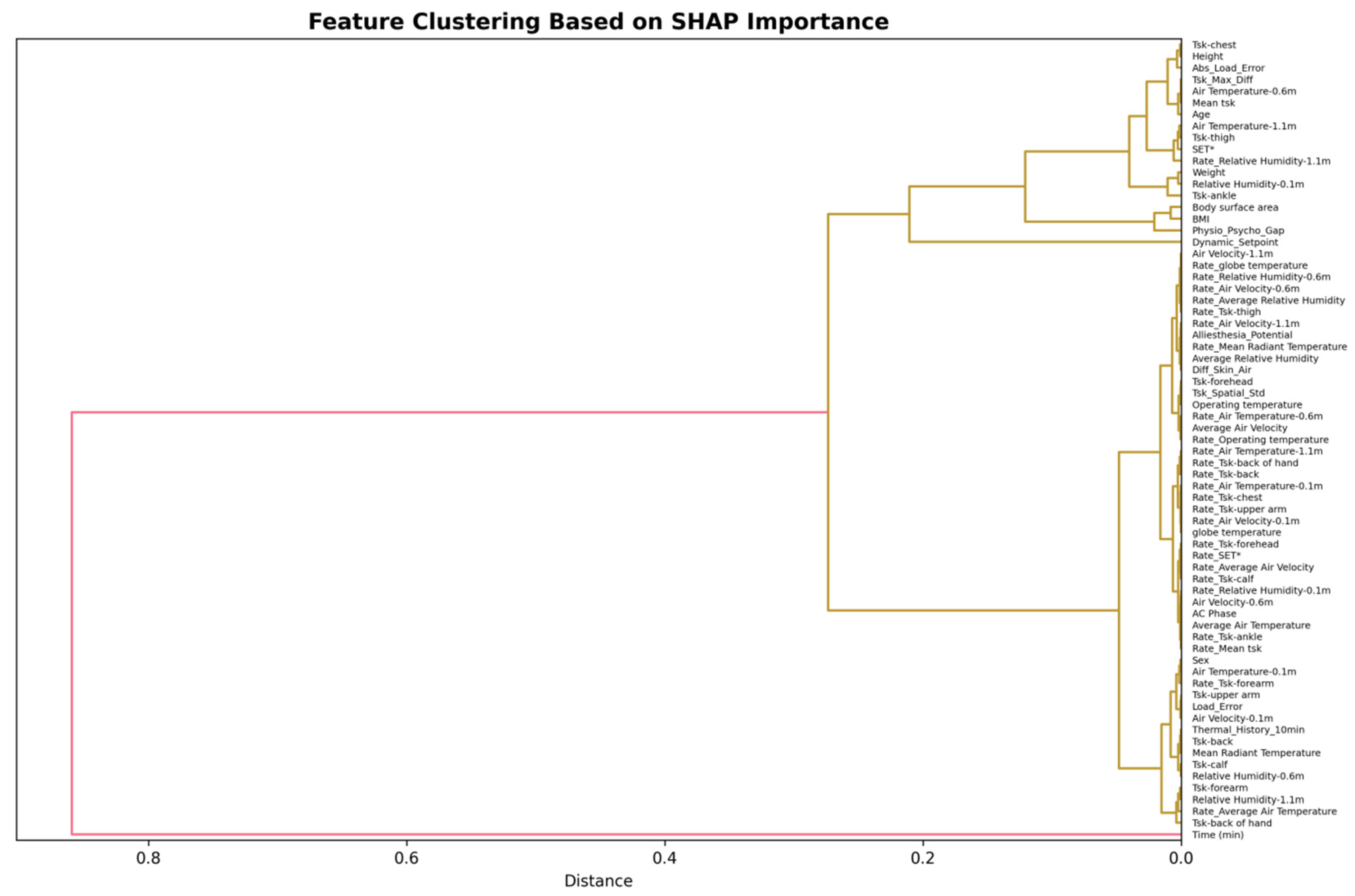
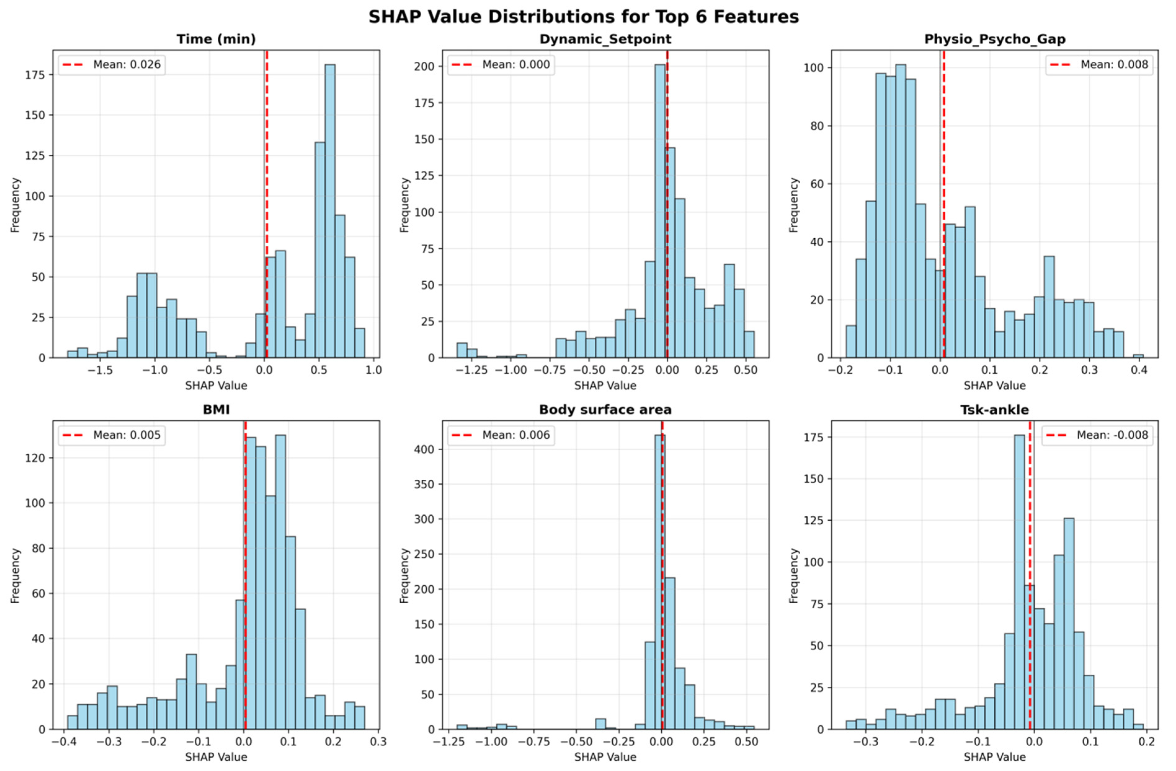
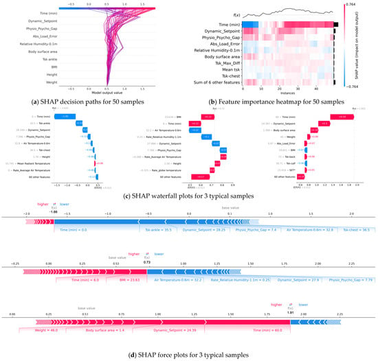
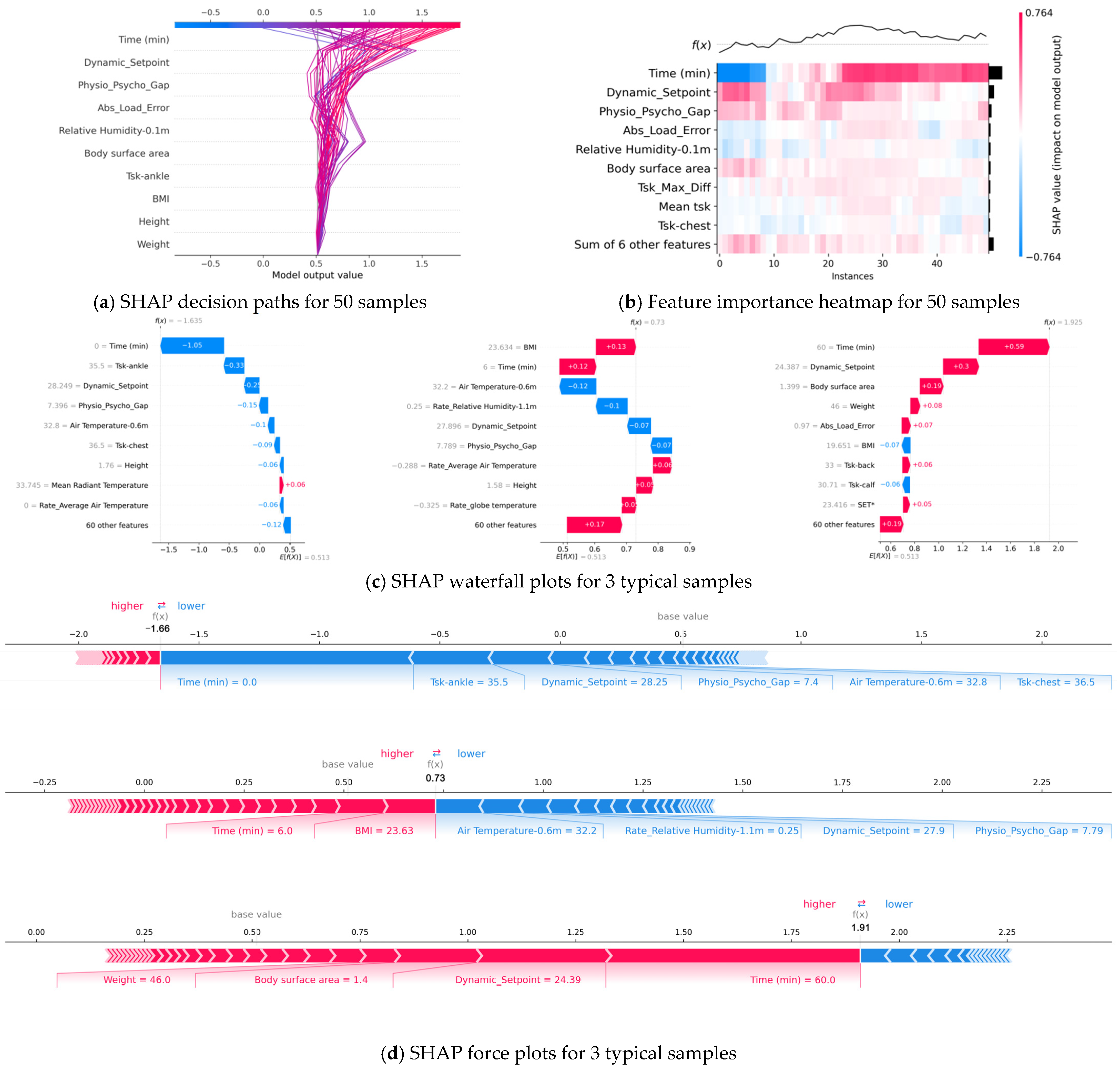

Disclaimer/Publisher’s Note: The statements, opinions and data contained in all publications are solely those of the individual author(s) and contributor(s) and not of MDPI and/or the editor(s). MDPI and/or the editor(s) disclaim responsibility for any injury to people or property resulting from any ideas, methods, instructions or products referred to in the content. |
© 2026 by the authors. Licensee MDPI, Basel, Switzerland. This article is an open access article distributed under the terms and conditions of the Creative Commons Attribution (CC BY) license.