Evaluation of Spatial Variability in Fecal Indicator Bacteria in Urban Recreational Lakes by One-Way ANOVA

Abstract

Urban recreational lakes require systematic microbiological monitoring to ensure public health protection and agreement with bathing-water regulations. This study investigates the spatial variability in fecal indicator bacteria (Escherichia coli and intestinal enterococci) at two major urban bathing sites in Zagreb, Croatia (Lake Bundek and Lake Jarun), using a four-year monitoring dataset (2016–2019) collected at 19 fixed sampling locations. E. coli was quantified using a miniaturized most probable number (MPN) method, while intestinal enterococci were determined by membrane filtration, following ISO standards. Microbiological concentrations were log₁₀-transformed and analyzed using one-way analysis of variance (ANOVA) to test for statistically significant differences among sampling locations within each lake. Variability in microbiological data was characterized using box-and-whisker plots, which appropriately represent dispersion and skewness typical of MPN- and CFU-based measurements. The results indicate predominantly homogeneous spatial distributions of both indicators, particularly at Lake Jarun, where no statistically significant differences among sampling locations were observed. In contrast, a statistically significant spatial difference in E. coli concentrations was detected at Lake Bundek, likely reflecting site-specific characteristics such as smaller lake size and more limited water exchange.

1. Introduction

Recreational waters play an important role in public health and quality of life, particularly in urban environments where lakes and artificial water bodies are widely used for swimming and leisure activities. However, such waters are also vulnerable to microbiological contamination originating from human activities, wildlife, surface runoff, and wastewater inputs. Exposure to contaminated bathing water may pose health risks to bathers, primarily through gastrointestinal illnesses and skin or ear infections, which highlights the importance of systematic microbiological monitoring and risk assessment areas [1,2,3].

The microbiological quality of bathing waters is commonly evaluated using Escherichia coli and intestinal enterococci as fecal indicator bacteria. These indicators are internationally known and form the basis of regulatory frameworks such as the European Union Bathing Water Directive (2006/7/EC), which classifies bathing waters into four quality categories (“excellent”, “good”, “sufficient”, and “poor”) based on percentile values of these parameters [4]. Continuous monitoring of microbiological indicators is therefore essential not only for ensuring regulatory compliance but also for protecting public health and informing lake management strategies.

Urban lakes represent particularly complex systems due to their heterogeneous spatial structure, varying hydrological conditions, and intense seasonal human use. Differences in lake size, water residence time, connectivity, and recreational pressure may lead to spatial variability in microbiological water quality within a single lake and between lakes [5,6,7]. Identifying whether such spatial differences are statistically significant is crucial for designing efficient monitoring programs and for understanding whether specific locations represent persistent hotspots of microbiological contamination [8].

Statistical methods are widely applied to evaluate spatial and temporal variability in water quality parameters. Among these, analysis of variance (ANOVA) remains a commonly used approach for testing whether differences between group means such as sampling locations are statistically significant. Despite the increasing availability of more advanced statistical and risk-based approaches in recreational water quality research, one-way ANOVA is still frequently applied in regulatory monitoring contexts, particularly when datasets are structured around fixed sampling locations and repeated seasonal measurements.

Recent international studies on microbiological monitoring of recreational waters have increasingly emphasized the importance of understanding spatial and temporal variability in fecal indicator concentrations to optimize monitoring strategies and improve risk assessment [8,9,10]. For instance, investigations in coastal and urban water bodies have employed statistical methods, including ANOVA, to quantify spatial heterogeneity, often finding limited significant differences among sites in larger, well circulated systems but localized variations in smaller or protected areas [11,12]. Advanced approaches, such as quantitative microbial risk assessment, Bayesian modeling, and predictive now casting, have been integrated with traditional indicator monitoring to enable more practical, risk-based management under the revised EU Bathing Water Directive and WHO guidelines [13,14,15,16]. These methods highlight the potential for reducing monitoring effort while maintaining public health protection, particularly in urban lakes where bather density and hydrodynamic factors can influence contaminant distribution. However, comparatively fewer studies have systematically examined spatial heterogeneity within and between urban lakes over multi-year monitoring periods while explicitly linking statistical findings to regulatory bathing water classifications [16,17,18].

The present study addresses this gap by analyzing a four-year dataset (2016–2019) of microbiological bathing water quality collected at two urban lakes in Zagreb, Lake Bundek and Lake Jarun which differ markedly in size, morphology and recreational use intensity. The study focuses on spatial differences in E. coli and intestinal enterococci concentrations across defined sampling locations within each lake.

The specific objectives of this study are to:

(i)

quantify the spatial variability in microbiological indicators (E. coli and intestinal enterococci) across sampling locations within each lake;

(ii)

test whether observed spatial differences are statistically significant using one-way ANOVA;

(iii)

compare microbiological patterns between two contrasting urban lakes; and

(iv)

interpret the results in the context of European bathing water quality standards.

The novelty of this work lies in its multiyear, spatially explicit comparison of microbiological bathing water quality at two urban lakes with contrasting characteristics, combined with a transparent statistical evaluation of spatial variability aligned with regulatory criteria. The results provide insight into whether routine monitoring locations adequately capture spatial heterogeneity and offer a practical case study relevant to urban lake management and bathing water assessment.

2. Experimental Part

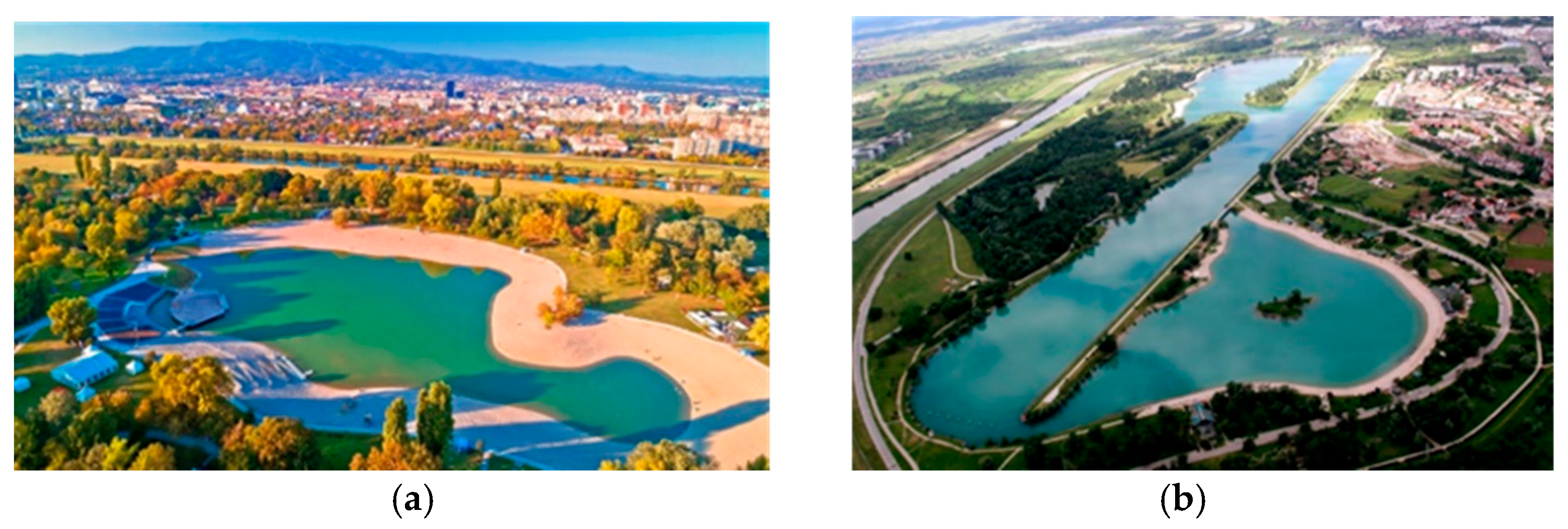
Lakes Bundek and Jarun (Figure 1) were selected for this study as they represent the two most popular and used urban recreational bathing sites in Zagreb, Croatia, attracting hundreds of thousands of visitors annually during the summer months. Lake Bundek is a small (≈0.2 km²), shallow artificial lake with limited water exchange, while Lake Jarun is significantly larger (≈0.6 km²) with multiple connected basins and better circulation. This contrast in morphology and hydrodynamic characteristics makes them ideal for comparing spatial variability in fecal indicator distribution under similar climatic conditions and recreational pressure [19,20].

Figure 1. (a) Lake Bundek; (b) Lake Jarun.

From a public health perspective, this study addresses the question of whether multiple fixed sampling points are justified within individual urban lakes, or whether water quality is sufficiently homogeneous to allow monitoring optimization without compromising safety. Reliable assessment of spatial heterogeneity supports evidence-based decisions on monitoring effort under the EU Bathing Water Directive [4], ultimately contributing to more efficient resource allocation while maintaining high protection standards for bathers.

2.1. Sampling

In order to monitor the quality of bathing water, it is necessary to conduct water sampling. Water sampling was carried out according to the Bathing Water Quality Regulation (NN 51/14) [21]. Prior to the sampling procedure, the sampling vials should be sterilized (15 min at 121 °C in an autoclave or 1 h by dry sterilization at 160–170° C). In addition to sterilizing existing sampling vessels, it is possible to use disposable sampling bottles, which have been previously sterilized by radiation. At the sampling point itself, the sample is taken with a hand-held sampler 30 cm below the surface of the water in water at least 1 m deep. The sampling bottle must have a volume of 250 mL made of transparent material and unpainted material (polypropylene, polyethylene or glass). Samples should be analyzed as soon as possible, and the longest period for laboratory analysis is within 24 h (before that, samples must be protected from light and temperature). For protection purposes, the sample is stored in a dark place at a temperature of 4 °C ± 3 °C. Sampling on Lake Bundek was carried out on the Great Lake at three locations B1, B2 and B3, i.e., on the eastern, western and southern shores. Sampling lasted for four years from 2016 to 2019 from June to September. Each month (except September) was sampled twice, except in August 2017 and 2019 in July when sampling was conducted three times. Sampling on Lake Jarun was carried out on the Big and Small Lakes. In the area of the Great and Small Lakes, it was caused by a total of 12 points, the first six on the Great Lake (TU 01, TU 02, TU 03, TU 04, TU 05, TU 06) and the next six on the Small Lake (TU 07, TU 08, TU 09, TU 10, TU 11, TU 12).

2.2. Determination of Microbiological Parameters

In order to determine microbiological contamination, the presence of fecal bacteria (Escherichia coli and intestinal enterococci) should be examined. Two methods for determining the number of bacteria were used to determine microbiological indicators of water quality. A miniaturized most probable number (MPN) method was used for E. coli, and a membrane filtration method was used for intestinal enterococci [22].

E. coli were quantified using the miniaturized most probable number (MPN) method according to HRN EN ISO 9308-3:2000 [23]. For each sample, 100 mL of water was pro-cessed using a standardized miniaturized MPN system. The sample was added to the reagent, mixed, and poured into a Quanti-Tray/2000 (providing 97 wells, 49 large wells of 10 mL and 48 small wells of 1 mL), which was then sealed and incubated at 36 ± 2 °C for 24–48 h. After incubation, wells exhibiting yellow colour (indicative of coliforms) and fluorescence under UV light at 366 nm, which is indicative for E. coli, were counted as positive. The MPN value was determined from the number of positive wells using the manufacturer’s MPN table or the standard’s statistical tables. Each sample was analyzed in a single technical replicate due to the high number of wells (97) providing inherent statistical robustness and no additional parallel trays were used.

For statistical analysis, raw MPN values (per 100 mL) were log₁₀-transformed to ap-proximate normality. We acknowledge that the variance of log-transformed MPN values can vary slightly depending on the number of positive wells; however, Levene’s test con-firmed homogeneity of variances across sampling sites (p > 0.05), indicating that this inherent feature of the MPN method did not substantially affect the validity of the one-way ANOVA results.

Intestinal enterococci were enumerated by the membrane filtration method according to HRN EN ISO 7899-2:2000 [24]. A volume of 100 mL (or appropriate dilutions for highly contaminated samples) was filtered through a 0.45 µm cellulose nitrate membrane filter. The filter was placed on Slanetz–Bartley agar and incubated at 36 ± 2 °C for 44 ± 4 h. Typical red, maroon or pink colonies were counted as presumptive intestinal enterococci. Where necessary, confirmation was performed by transferring colonies to bile aesculin agar and incubating at 44 °C for 2 h (darkening indicative of confirmation). Results were expressed as colony forming units (CFU) per 100 mL. Triplicate filtrations were not routinely performed because each sample was filtered once, in line with standard monitoring protocols for bathing waters. All analyses were completed within 24 h of sampling.

Colony counts from membrane filtration were treated as direct enumerations (CFU/100 mL). All microbiological concentrations were originally expressed per 100 mL, following regulatory standards. For statistical analysis, these values were mathematically converted to per mL units (CFU mL⁻¹, MPN mL⁻¹), and log₁₀-transformed accordingly. Variability among samples is fully represented by the box-and-whisker plots.

2.3. Method-Statistical Analysis

Statistical analysis was performed to examine whether microbiological indicator concentrations differed significantly among sampling locations within each lake. Separate analyses were conducted for Escherichia coli and intestinal enterococci, and for each lake system (Lake Bundek, Great Lake Jarun and Small Lake Jarun).

Prior to analysis, microbiological concentrations were log₁₀-transformed to improve normality and stabilize variance, which is standard practice for fecal indicator bacteria data. The transformed values are expressed as log₁₀(CFU/100 mL).

2.3.1. Statistical Frame

A one-way analysis of variance (ANOVA) was applied with sampling location as the fixed factor. The statistical frame was defined as follows:

• Response variables: log₁₀(E. coli) and log₁₀(intestinal enterococci) [CFU/100 mL]
• Fixed factor: Sampling location
• Factor levels: Lake Bundek: 3 locations (B1–B3)
  • Great Lake Jarun: 6 locations (TU01–TU06)
  • Small Lake Jarun: 6 locations (TU07–TU12)
• Sample size: A total of 465 samples were analysed for each microbiological indicator across the study period (2016–2019).
• Significance level: α = 0.05

Analyses were performed separately for each lake and indicator to avoid confounding effects related to differences in lake morphology and usage.

2.3.2. Assumptions and Diagnostic Tests

The assumptions underlying one-way ANOVA were evaluated prior to hypothesis testing:

• Independence of observations was ensured by sampling at spatially distinct locations and by treating each sampling event as an independent observation. Because samples at each location were collected on distinct dates over multiple bathing seasons, with substantial temporal separation and under varying meteorological and hydrological conditions, individual observations can be reasonably treated as approximately independent realizations, allowing all years to be pooled for an overall one-way ANOVA focused on average spatial differences.
• Normality of residuals was assessed using the Shapiro–Wilk test applied to log-transformed data. Most datasets showed statistically significant deviations from normality (p < 0.05), particularly when all sampling locations and years were pooled (W = 0.875–0.921, p < 0.001). However, smaller subsets (e.g., single-year data from Lake Bundek with n ≈ 30–31 per location) were closer to normal distribution (p = 0.118 for E. coli and p = 0.341 for enterococci in 2016), allowing borderline acceptance of normality in some cases. Despite these deviations, one-way ANOVA was applied because ANOVA is known to be robust against moderate departures from normality when sample sizes are similar across groups and sufficiently large (n ≥ 25–30 per group), as was the case in this study. The nonparametric Kruskal-Wallis test, performed as a sensitivity analysis, yielded nearly identical conclusions regarding the presence or absence of significant spatial differences between sampling locations. Log-transformation substantially reduced asymmetry of the distributions. Therefore, the parametric approach was considered appropriate and the results were interpreted with confidence, supported by the consistency with the nonparametric equivalent.
• Homogeneity of variances was evaluated using Levene’s test. The test results confirmed that variances among sampling locations were not significantly different (p > 0.05), supporting the use of ANOVA.
• No data points were excluded from the analysis. Values identified as extreme in boxplot visualisations were retained, as they represent environmentally relevant observations rather than measurement errors.

2.3.3. Hypothesis Testing and Post Hoc Analysis

For each analysis, the null hypothesis (H₀) stated that the mean microbiological concentration was equal across all sampling locations within a lake, while the alternative hypothesis (H₁) stated that at least one location differed significantly.

The ANOVA F-test was used to evaluate the null hypothesis. Statistical significance was determined using the decision rule:

• if p < α (0.05), H₀ was rejected and a significant spatial difference was inferred;
• if p ≥ α, H₀ was not rejected and no significant spatial difference was concluded.

When a statistically significant result was obtained, post hoc pairwise comparisons were performed using Tukey’s Honestly Significant Difference (HSD) test to identify which sampling locations contributed to the observed difference. This method was selected because it controls the family-wise error rate and is appropriate for approximately balanced sample sizes.

2.3.4. Software

All statistical analyses were conducted using the Data Analysis Toolpak in Microsoft Excel (Microsoft 365). The software was used to calculate ANOVA F-statistics, p-values, and post hoc comparisons. The level of statistical significance was consistently set at α = 0.05 for all tests.

3. Results and Discussion

Each year, EU Member States are required to identify the bathing waters within their territory and define the duration of the bathing season. Monitoring must be established at the locations most frequently used by bathers or at sites where the risk of contamination is highest. Monitoring is carried out by sampling at least four samples per season, including one taken before the start of the bathing season and three samples only if the bathing season does not exceed eight weeks or if the area is subject to specific geographical constraints. The microbiological quality of bathing waters is classified using intestinal enterococci and Escherichia coli as indicator organisms. Threshold values for “excellent,” “good,” and “sufficient” water quality are 200, 400, and 330 CFU/100 mL for intestinal enterococci, and 500, 1000, and 900 CFU/100 mL for E. coli, respectively. These parameters are determined using standardized analytical methods.

3.1. Descriptive Statistics

The examination of microbiological indicators was conducted at two locations in the city of Zagreb, on Lake Bundek and Jarun. Three sampling points (B1, B2 and B3) were defined on Lake Bundek, while 12 sampling points were defined on Lake Jarun (TU 01, TU 02, TU 03, TU 04, TU 05, TU 06, TU 07, TU 08, TU 09, TU 10, TU 11, TU 12). Sampling was conducted over four years, from 2016 to 2019. Sampling was conducted every year from June to September, except in 2016 when the first sampling was in April. Figure 2, Figure 3, Figure 4, Figure 5, Figure 6, Figure 7, Figure 8 and Figure 9 show log₁₀-transformed concentrations (CFU/100 mL) for individual measurements, while Figure 10, Figure 11, Figure 12, Figure 13, Figure 14 and Figure 15 summarize these data using box-and-whisker plots for each sampling location. For both MPN and CFU based data, central tendency and dispersion are presented using medians and interquartile ranges rather than means with error bars, in order to avoid misleading interpretation caused by skewed distributions and occasional extreme values typical of microbiological data.

Figure 2 shows E. coli concentrations for 2016 with low variability (narrow spread) across sampling locations, indicating that values are relatively similar. In particular, locations TU05 and TU12 exhibit a narrow range of values, indicating similar E. coli levels at these sites.

Figure 2. Log₁₀-transformed concentrations of E. coli (CFU/100 mL) for individual sampling measurements at each sampling location in Lake Bundek and Lake Jarun in 2016.

Figure 2. Log₁₀-transformed concentrations of E. coli (CFU/100 mL) for individual sampling measurements at each sampling location in Lake Bundek and Lake Jarun in 2016.

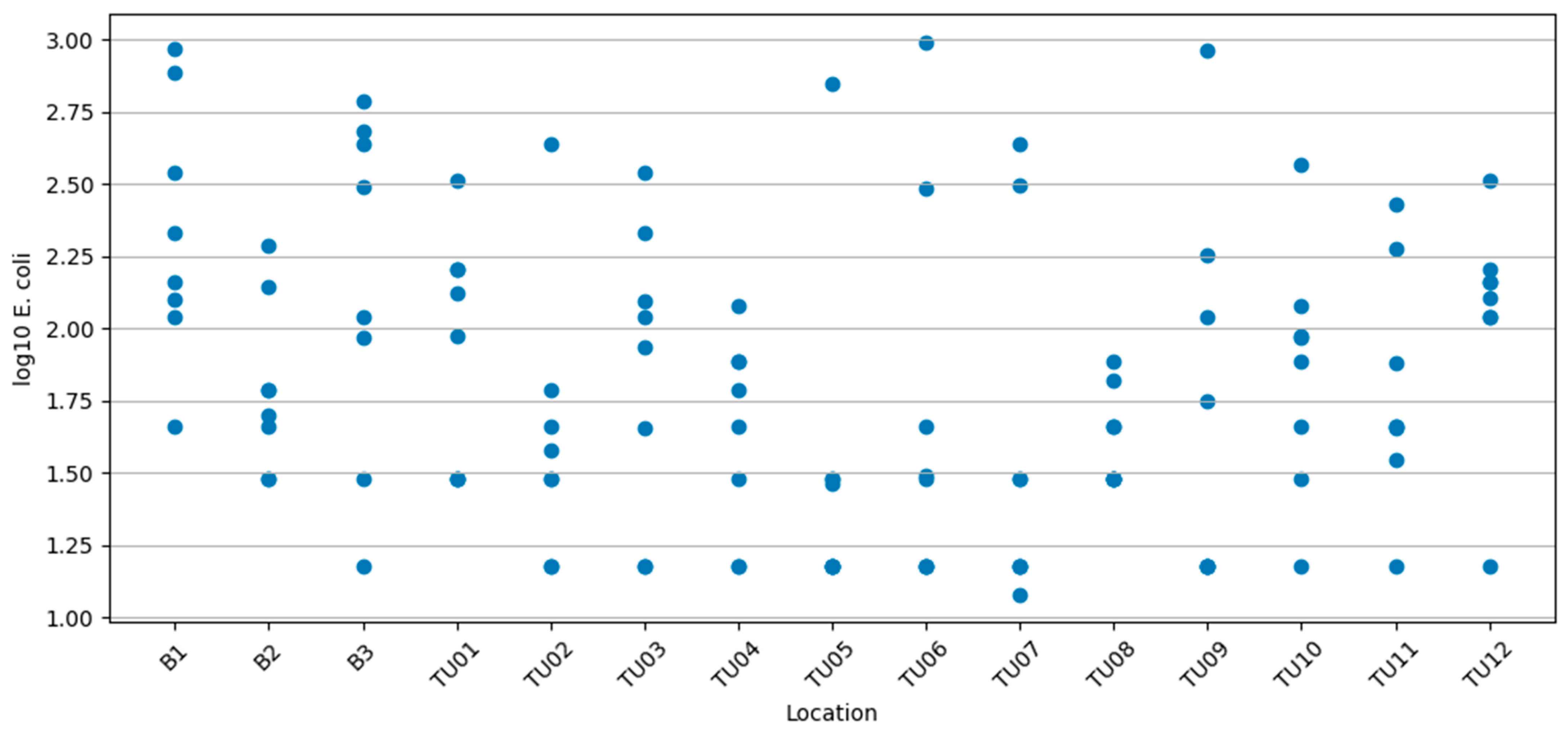
Figure 3 shows greater variability (wider spread) of E. coli concentrations across sites compared with 2016. The values are more widely dispersed among sites, reflecting larger differences in E. coli concentrations. In particular, locations B2 and TU01 exhibit higher concentrations, whereas lower concentrations are observed at TU01 and TU03.

Figure 3. Log₁₀-transformed concentrations of E. coli (CFU/100 mL) for individual sampling measurements at each sampling location in Lake Bundek and Lake Jarun in 2017.

Figure 3. Log₁₀-transformed concentrations of E. coli (CFU/100 mL) for individual sampling measurements at each sampling location in Lake Bundek and Lake Jarun in 2017.

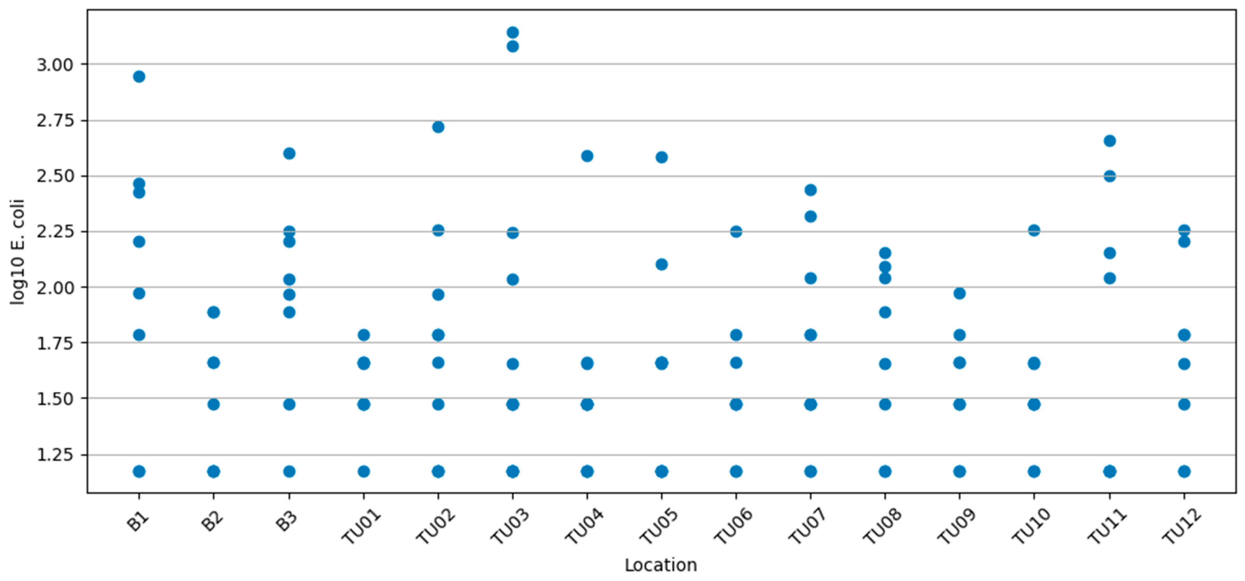
Figure 4, which shows E. coli concentrations for 2018, indicates a reduced variability (narrower spread) across sampling locations compared with previous years. In particular, the lowest concentrations are observed at locations TU05 and TU07.

Figure 4. Log₁₀-transformed concentrations of E. coli (CFU/100 mL) for individual sampling measurements at each sampling location in Lake Bundek and Lake Jarun in 2018.

Figure 4. Log₁₀-transformed concentrations of E. coli (CFU/100 mL) for individual sampling measurements at each sampling location in Lake Bundek and Lake Jarun in 2018.

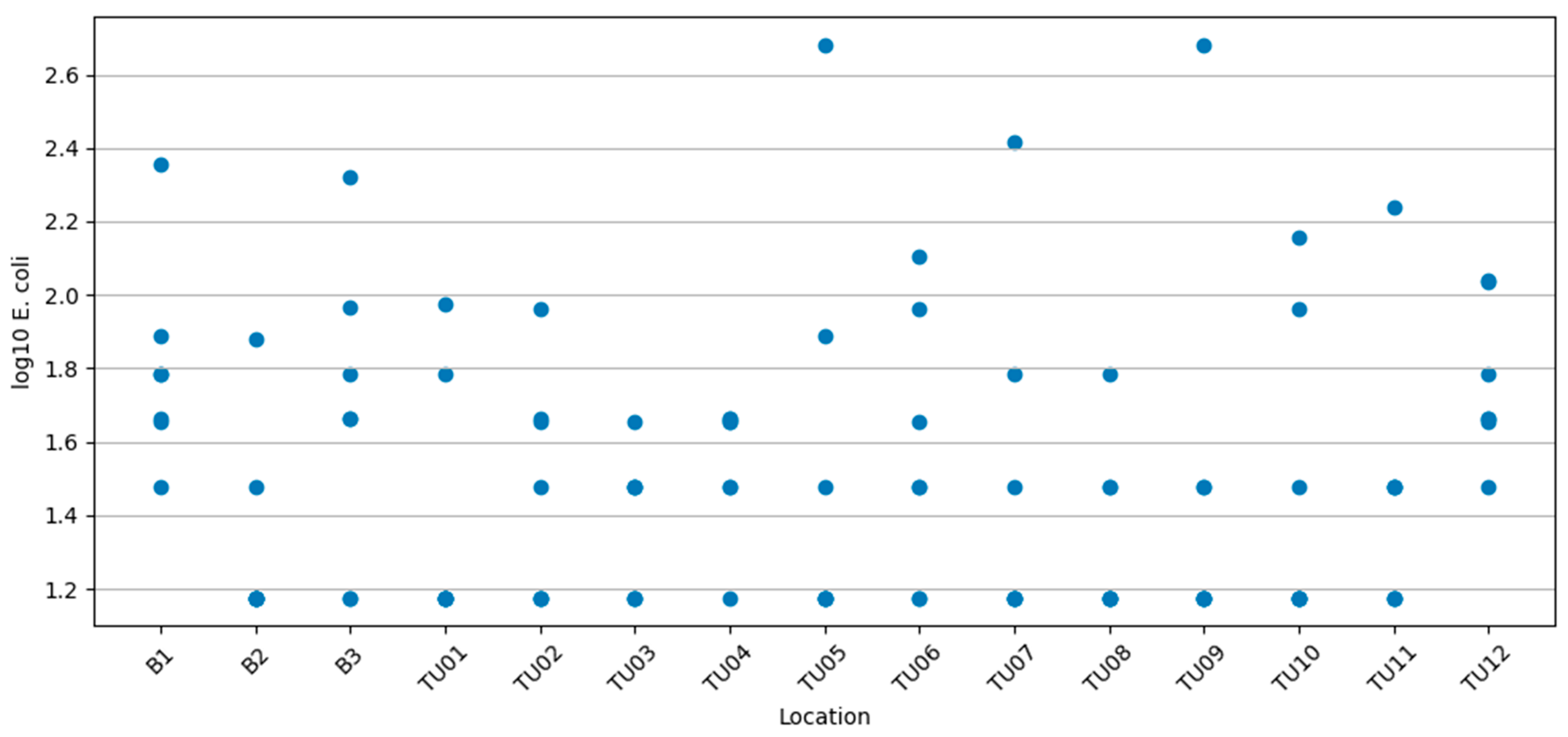
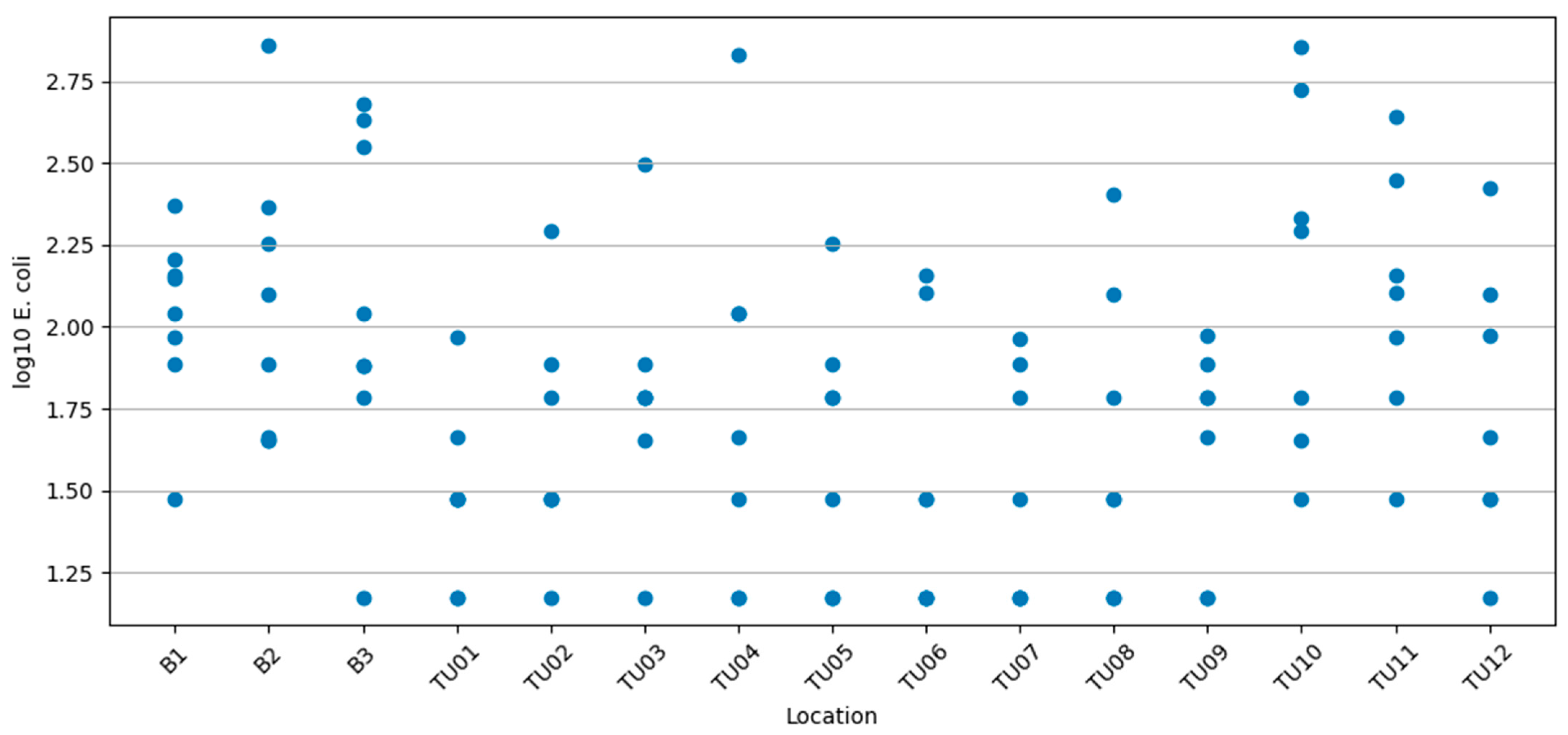
Figure 5 shows relatively low E. coli concentrations, with the lowest values observed at locations TU04 and TU12. Over the four-year period, the variability and overall level of E. coli concentrations decrease, indicating an overall improvement in microbiological water quality.

Figure 5. Log₁₀-transformed concentrations of E. coli (CFU/100 mL) for individual sampling measurements at each sampling location in Lake Bundek and Lake Jarun in 2019.

Figure 5. Log₁₀-transformed concentrations of E. coli (CFU/100 mL) for individual sampling measurements at each sampling location in Lake Bundek and Lake Jarun in 2019.

A comparison of Figure 2 (2016) and Figure 3 (2017) shows a reduction in the variability and overall level of E. coli concentrations over time. The decrease in E. coli concentrations from 2016 to 2019 indicates an overall improvement in microbiological water quality. This trend may be related to several factors, including changes in bather numbers and recreational activities, improved water quality management, increased water exchange and dilution, as well as inter-annual and seasonal meteorological variability. However, these factors were not included as quantitative predictors in the present statistical analysis and are therefore discussed only as probable contributors rather than demonstrated causes.

Although the boxplots show some visual variability among sampling points at Great and Small Lake Jarun, one-way ANOVA demonstrates that these differences are not statistically significant. This indicates a spatially homogeneous distribution of E. coli across the Jarun basins, consistent with a well-mixed water body and distributed contamination sources rather than localized hotspots.

Figure 6 shows intestinal enterococci concentrations for 2016, with relatively low variability across sampling locations. In particular, locations TU01 and TU03 show lower concentrations.

Figure 6. Log₁₀-transformed concentrations of intestinal enterococci (CFU/100 mL) for individual sampling measurements at each sampling location in Lake Bundek and Lake Jarun in 2016.

Figure 6. Log₁₀-transformed concentrations of intestinal enterococci (CFU/100 mL) for individual sampling measurements at each sampling location in Lake Bundek and Lake Jarun in 2016.

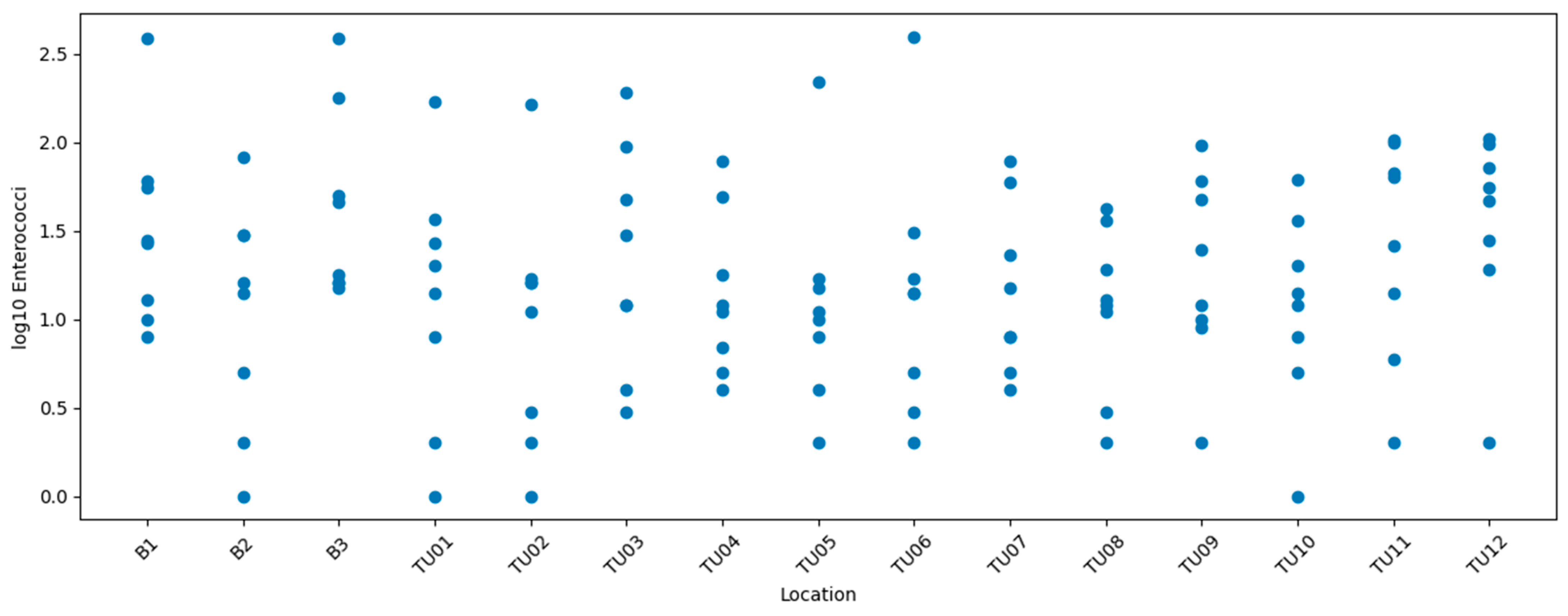
Figure 7 shows higher intestinal enterococci concentrations at locations TU05 and TU07, while lower concentrations are observed at TU03.

Figure 7. Log₁₀-transformed concentrations of intestinal enterococci (CFU/100 mL) for individual sampling measurements at each sampling location in Lake Bundek and Lake Jarun in 2017.

Figure 7. Log₁₀-transformed concentrations of intestinal enterococci (CFU/100 mL) for individual sampling measurements at each sampling location in Lake Bundek and Lake Jarun in 2017.

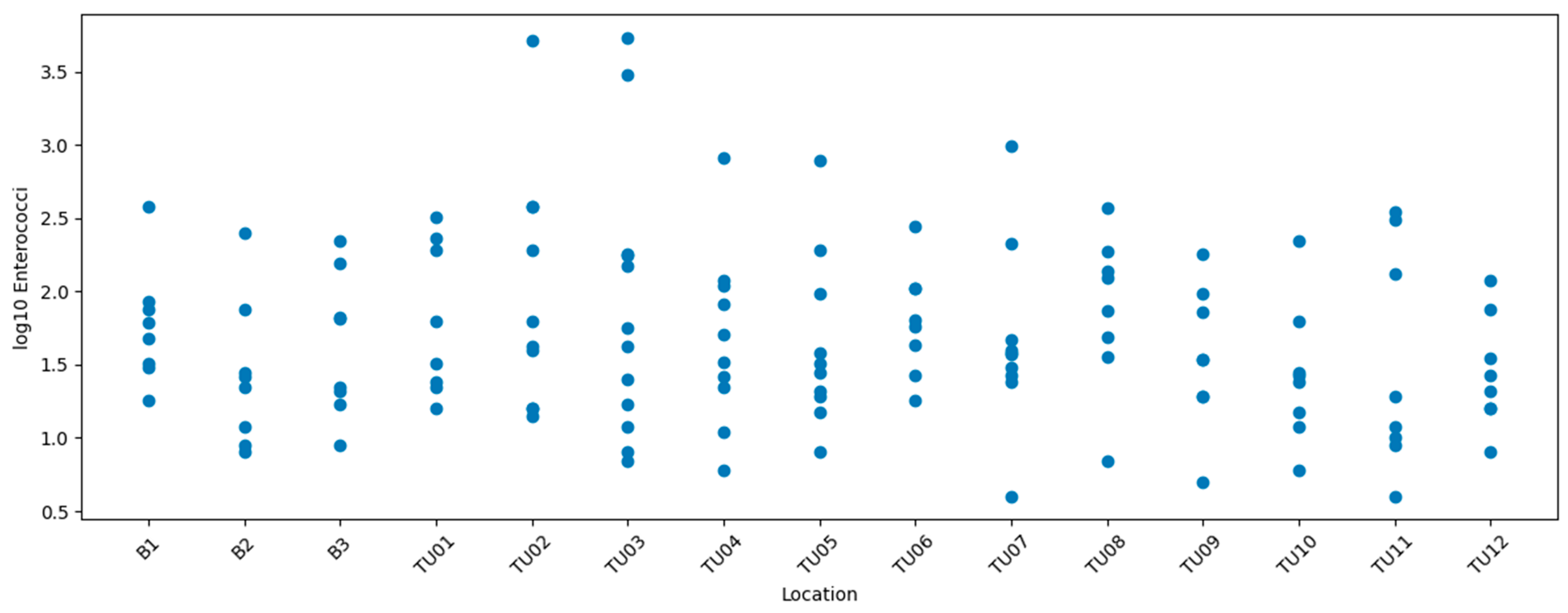
The results shown in Figure 8 indicate increased intestinal enterococci concentrations, with the highest values observed at locations TU02 and TU03.

Figure 8. Log₁₀-transformed concentrations of intestinal enterococci (CFU/100 mL) for individual sampling measurements at each sampling location in Lake Bundek and Lake Jarun in 2018.

Figure 8. Log₁₀-transformed concentrations of intestinal enterococci (CFU/100 mL) for individual sampling measurements at each sampling location in Lake Bundek and Lake Jarun in 2018.

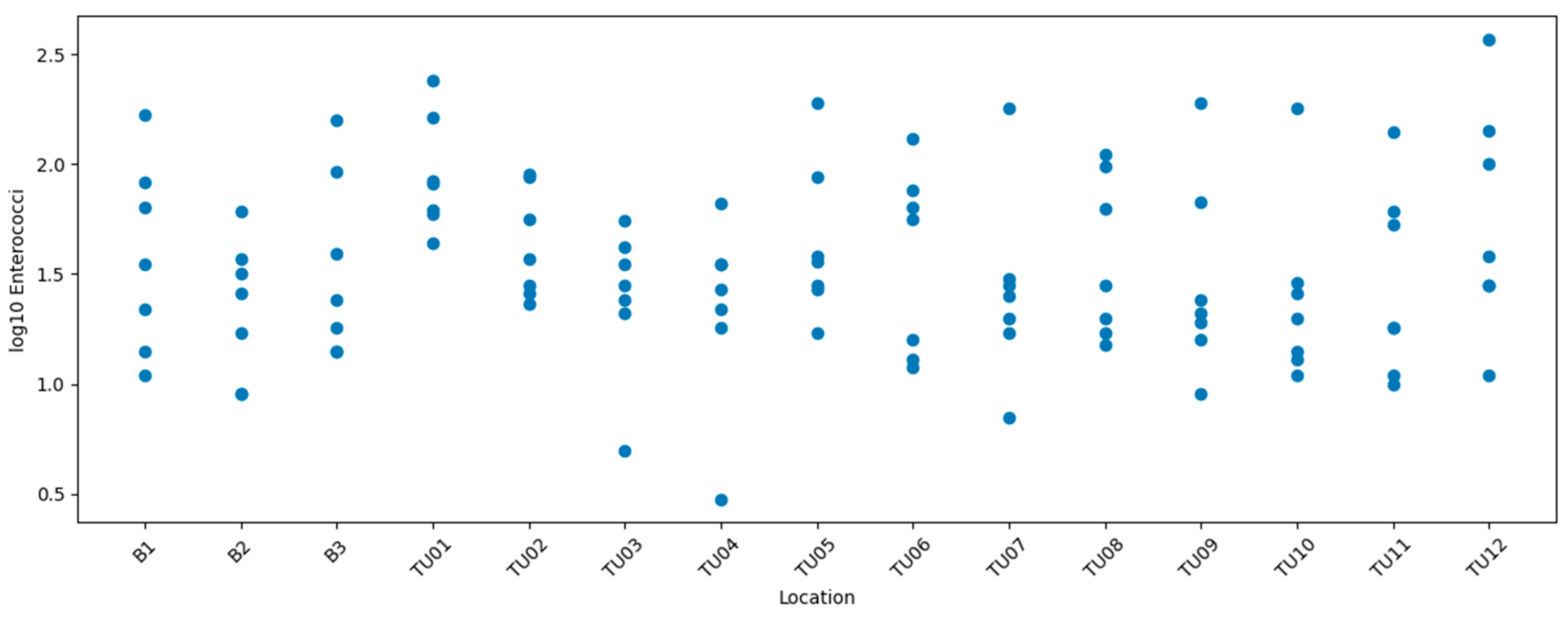
Figure 9 illustrates particularly high intestinal enterococci concentrations, with peak values observed at locations B2 and TU04.

Figure 9. Log₁₀-transformed concentrations of intestinal enterococci (CFU/100 mL) for individual sampling measurements at each sampling location in Lake Bundek and Lake Jarun in 2019.

Figure 9. Log₁₀-transformed concentrations of intestinal enterococci (CFU/100 mL) for individual sampling measurements at each sampling location in Lake Bundek and Lake Jarun in 2019.

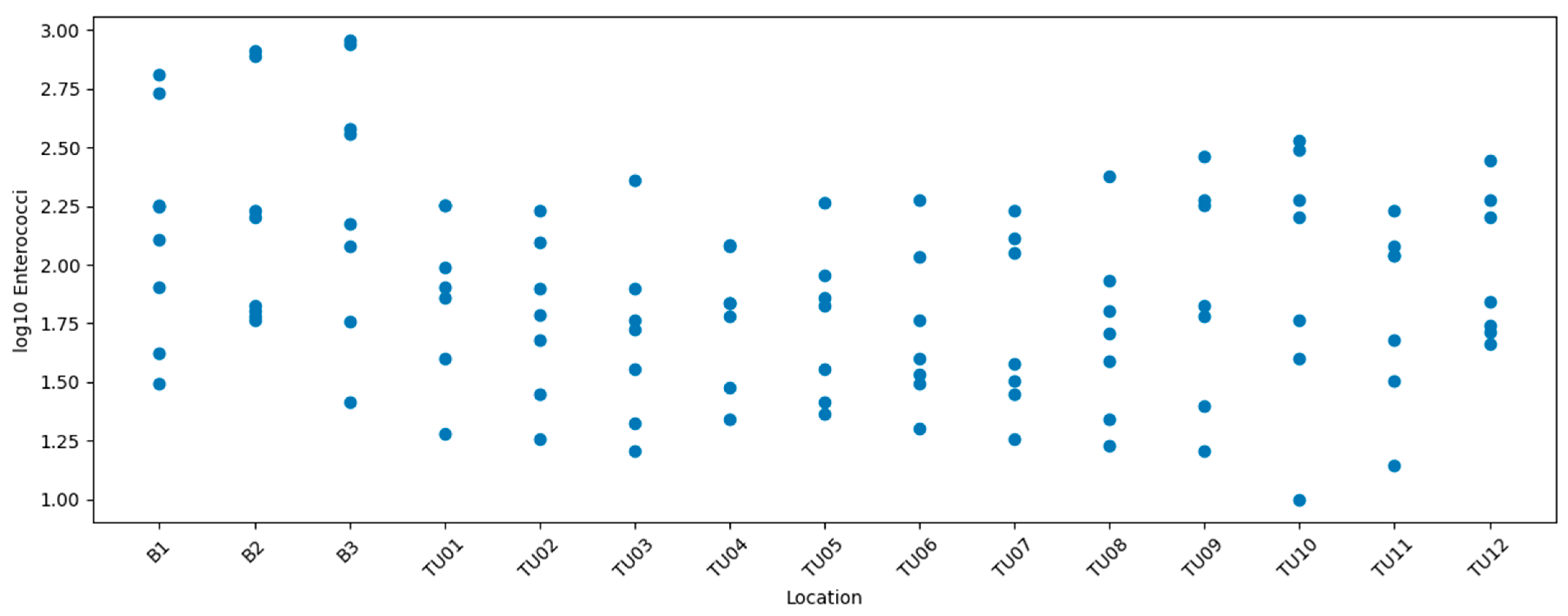
Over the four-year period, intestinal enterococci concentrations show an increasing trend. A comparison of Figure 6 (2016) and Figure 9 (2019) indicates higher overall levels in 2019. This increase may be related to several factors, including changes in bather numbers and rising average temperatures; however, these factors were not included as quantitative predictors in the statistical analysis and are therefore considered only as potential contributing factors rather than demonstrated causes.

The computed logarithmic values of E. coli and intestinal enterococci are the starting point for investigating how microbiological indicators of water quality are influenced by the sampling site [25,26]. Table 1 presents the arithmetic mean values of the logarithmic values of E. coli and intestinal enterococci throughout the four-year examination period at the sites of Lakes Bundek and Jarun.

Table 1. Values of the arithmetic mean of E. coli and intestinal enterococci for the period from 2016 to 2019.

Location	Arithmetic Mean (log10 E. coli)	Location	Arithmetic Mean (log10 Intestinal Enterococci)
B1	2.05508	B1	1.752095
B2	1.68057	B2	1.498872
B3	1.97527	B3	1.78066
TU 01	1.582943	TU 01	1.66786
TU 02	1.62532	TU 02	1.600568
TU 03	1.71827	TU 03	1.61636
TU 04	1.61365	TU 04	1.49078
TU 05	1.57161	TU 05	1.52082
TU 06	1.59633	TU 06	1.546847
TU 07	1.58972	TU 07	1.502533
TU 08	1.58771	TU 08	1.5492
TU 09	1.59623	TU 09	1.534743
TU 10	1.752	TU 10	1.450347
TU 11	1.7709	TU 11	1.54305
TU 12	1.81728	TU 12	1.667085

In Table 1, the highest values of the arithmetic mean are highlighted in red, while the lowest values of the arithmetic mean are highlighted in green. The highest arithmetic mean value for E. coli is recorded at sampling point B1, situated on the eastern shore of Lake Bundek, whereas the lowest value is found at point TU 08, located at Lake Jarun. The highest arithmetic mean value of the number of intestinal enterococci is found at sampling point B3, which is positioned on the southern shore of Lake Bundek, while the lowest value is again at point TU 10 at Lake Jarun. Based on the results obtained, it can be inferred that the arithmetic means are influenced by the size and usage of both lakes [25,26,27,28,29]. Lake Bundek has a smaller area in comparison to Lake Jarun, and its water temperature is approximately 2 °C higher, which promotes the growth of bacteria and algae.

Table 2 provides a concise numerical summary of log₁₀-transformed concentrations of Escherichia coli and intestinal enterococci for each sampling location and year, including measures of central tendency (mean and median), dispersion (standard deviation), range (minimum and maximum), and the percentage of samples exceeding EU bathing water standards (500 CFU/100 mL for E. coli and 200 CFU/100 mL for intestinal enterococci).

Table 2. Descriptive statistics of log₁₀-transformed fecal indicator bacteria concentrations by sampling location and year (2016–2019), (a) Escherichia coli and (b) intestinal enterococci.

(a) E. coli
Lake	Year	Mean (log10)	Median (log10)	SD (log10)	% >500	N
Bundek	2016	2.164	2.123	0.456	13.6	22
Bundek	2017	1.827	1.886	0.512	4.2	24
Bundek	2018	1.644	1.663	0.365	0	19
Bundek	2019	2.055	2.041	0.4	4.2	24
Jarun	2016	1.754	1.663	0.451	2.8	107
Jarun	2017	1.673	1.565	0.461	2.1	140
Jarun	2018	1.517	1.477	0.349	0	110
Jarun	2019	1.684	1.658	0.421	2.7	112
(b) Intestinal enterococci
Lake	Year	Mean (log10)	Median (log10)	SD (log10)	% >200	N
Bundek	2016	1.458	1.439	0.56	9.1	22
Bundek	2017	1.606	1.491	0.468	12.5	24
Bundek	2018	1.479	1.415	0.394	0	19
Bundek	2019	2.21	2.19	0.488	33.3	24
Jarun	2016	1.283	1.204	0.514	2.8	107
Jarun	2017	1.713	1.613	0.602	16.4	140
Jarun	2018	1.592	1.544	0.393	2.7	110
Jarun	2019	1.812	1.796	0.376	8	112

This table complements the graphical representations shown in Figure 2, Figure 3, Figure 4, Figure 5, Figure 6, Figure 7, Figure 8 and Figure 9 by quantifying interannual variability and highlighting the frequency of regulatory exceedances, thereby providing additional context for the subsequent ANOVA-based assessment of spatial differences among sampling locations.

The descriptive statistics indicate variability in microbiological concentrations across sampling locations. Table 2 indicates that most location/year combinations achieved excellent or good water quality status, confirming generally favourable microbiological conditions. This result indicates a generally high microbiological quality of the bathing waters, while also demonstrating pronounced spatial and temporal variability across monitoring locations and years. However, whether these differences represent true spatial heterogeneity is evaluated by the inferential analysis presented in Section 3.2.

3.2. One-Factor Analysis of Variance

During the timeframe from 2016 to 2019, a total of 465 samples were collected for the assessment of the levels of E. coli and intestinal enterococci. For each indicator, 93 samples were evaluated at Lake Bundek, 182 at Small Lake Jarun, and 190 at Great Lake Jarun. Given the extensive number of samples collected, that is, the data obtained, the calculated logarithmic values are represented in a box diagram for each microbiological indicator individually. Boxes show the interquartile range (25th–75th percentile), the horizontal line indicates the median, and whiskers represent the minimum and maximum values; points beyond the whiskers denote outliers. Mean values and associated variability are as mean ± standard deviation or standard error, because variability is explicitly represented by the box-and-whisker plots (interquartile range, median, and full data spread). This non-parametric visualization is appropriate for microbiological count data, which are typically non-normally distributed even after log transformation.

3.2.1. The Amount of Escherichia coli in Lakes Bundek and Jarun

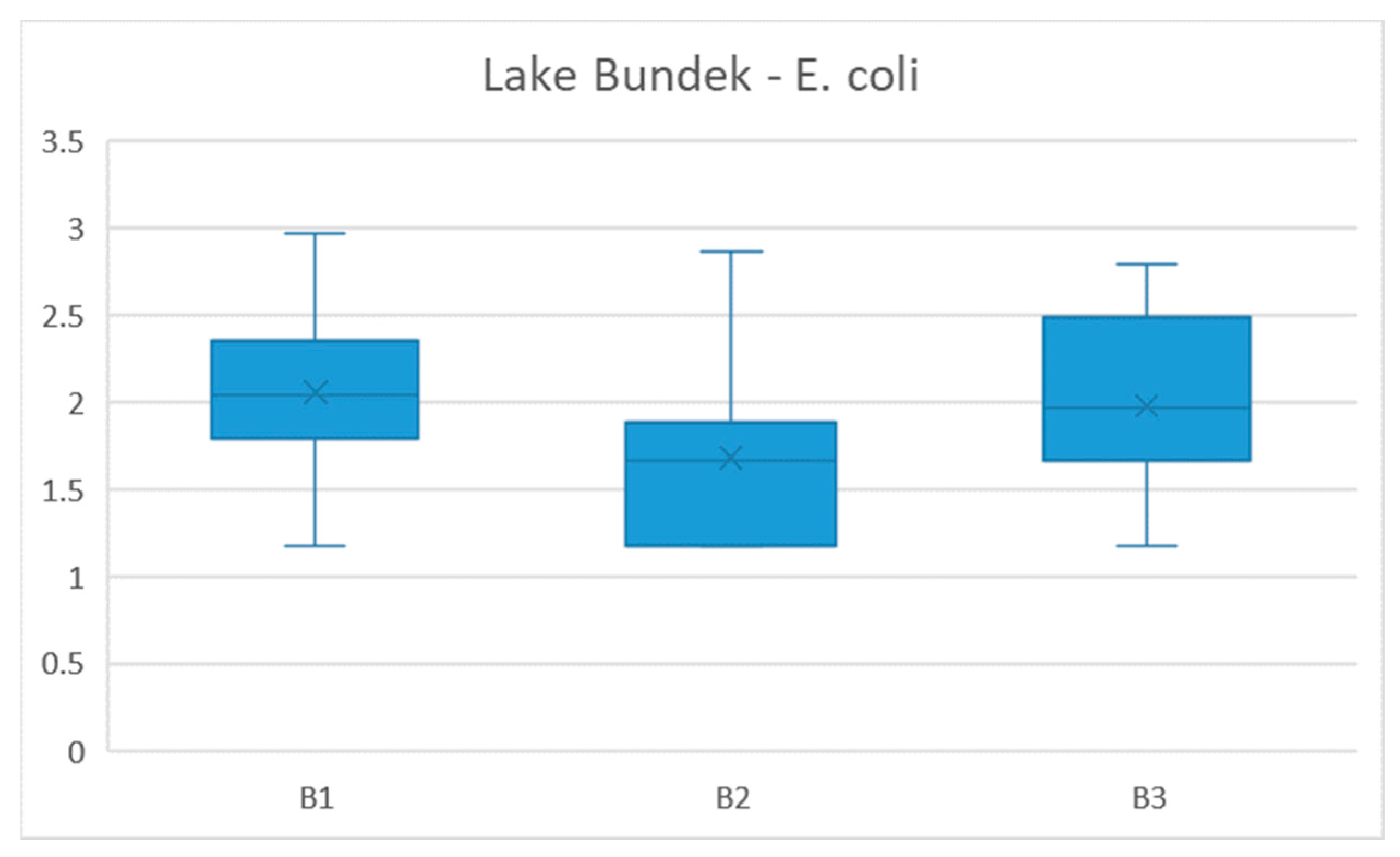
A total of 93 samples were collected at Lake Bundek at three locations: B1 on the east coast, B2 on the west coast, and B3 on the south coast—specifically, 31 samples from each location. The computed logarithmic values of the concentration of E. coli in Lake Bundek are illustrated by a box diagram in Figure 10. A box diagram is a graphical representation employed to depict the maximum, minimum, upper and lower quartiles, and median data. The horizontal line within the rectangle signifies the median (central value), whereas the horizontal lines (whiskers) outside the rectangle denote the largest and the smallest data points within the range [26,27,28,29,30]. The dots that appear above or below the whiskers signify values that deviate from the rest.

Figure 10 illustrates the distribution of E. coli at sites B1, B2, and B3. For all three locations, the minimum and maximum range from 1.2 to approximately 3.00. The average quantities of E. coli for points B1, B2, and B3 are 2.055, 1.681, and 1.975, respectively. At location B1, the distribution is symmetrical, whereas at location B2, it is skewed to the left and at B3 to the right. The occurrence of distribution skew is attributed to the uneven distribution of data.

Figure 10. Box-and-whisker plot of log₁₀-transformed E. coli concentrations (CFU/100 mL) at sampling locations B1–B3 on Lake Bundek (2016–2019).

Figure 10. Box-and-whisker plot of log₁₀-transformed E. coli concentrations (CFU/100 mL) at sampling locations B1–B3 on Lake Bundek (2016–2019).

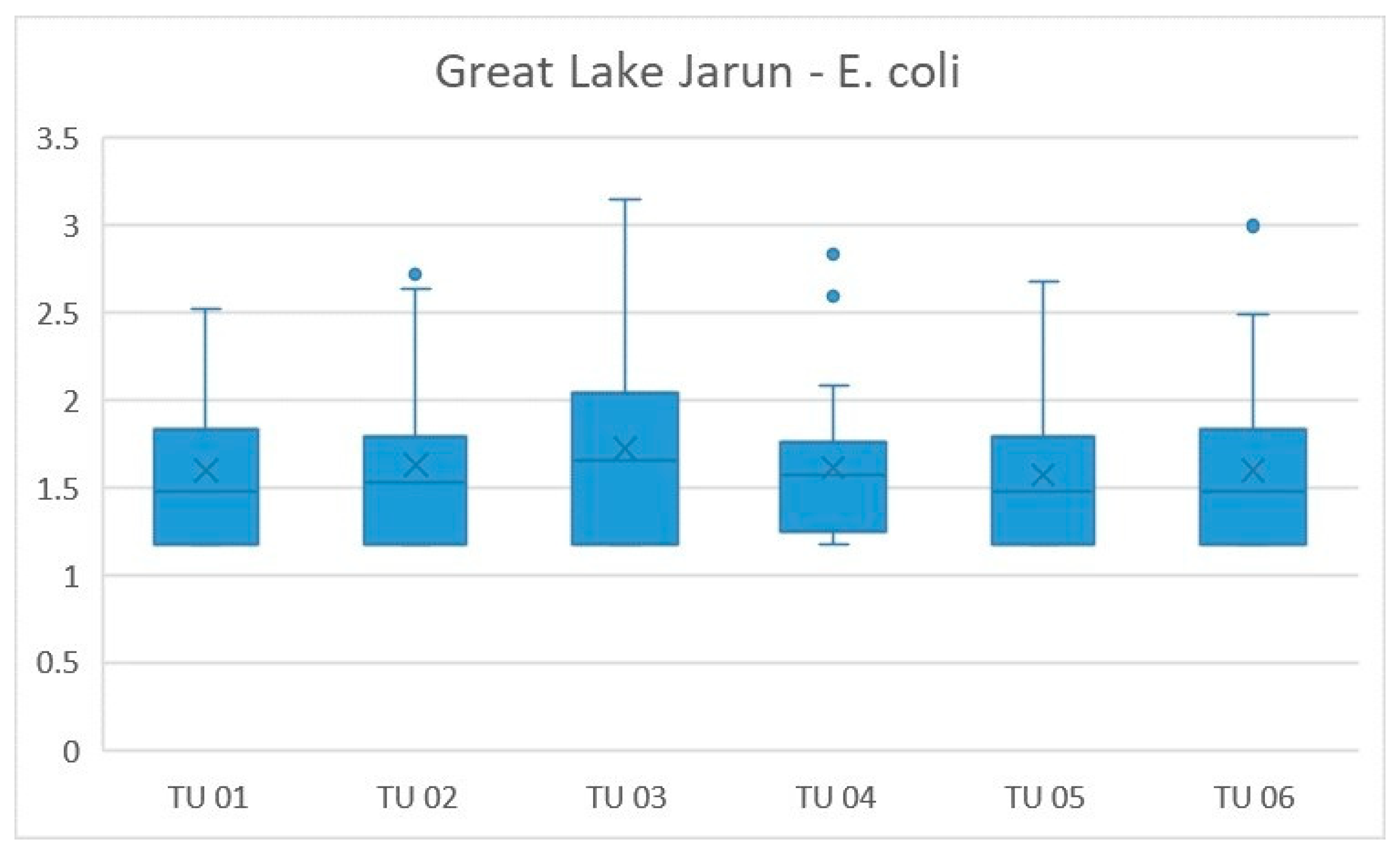
A total of 190 samples from six locations TU 01 30 samples, TU 02 31 samples, TU 03 34 samples, TU 04 32 samples, TU 05 32 samples and TU 06 30 samples were sampled at the Great Lake Jarun. The calculated logarithmic values of the amount of E. coli on the Great Lake Jarun are shown in a box diagram (Figure 11).

Figure 11 illustrates the minimum concentration of E. coli, which is 1.2 across all locations. The maximum concentrations of E. coli vary between 2.1 and 3.1. The mean concentrations of E. coli for points TU 01, TU 02, TU 03, TU 04, TU 05, and TU 06 range from 1.571 to 1.715. At locations TU 02, TU 04, TU 05, and TU 06, dots appear above the whisker, which signify information that diverges from the other data. At all locations, the distribution is symmetrical, with the exception of TU 03 and TU 04, where it is skewed to the left.

Figure 11. Box-and-whisker plot of log₁₀-transformed E. coli concentrations (CFU/100 mL) at sampling locations B1–B3 on Great Lake Jarun (2016–2019).

Figure 11. Box-and-whisker plot of log₁₀-transformed E. coli concentrations (CFU/100 mL) at sampling locations B1–B3 on Great Lake Jarun (2016–2019).

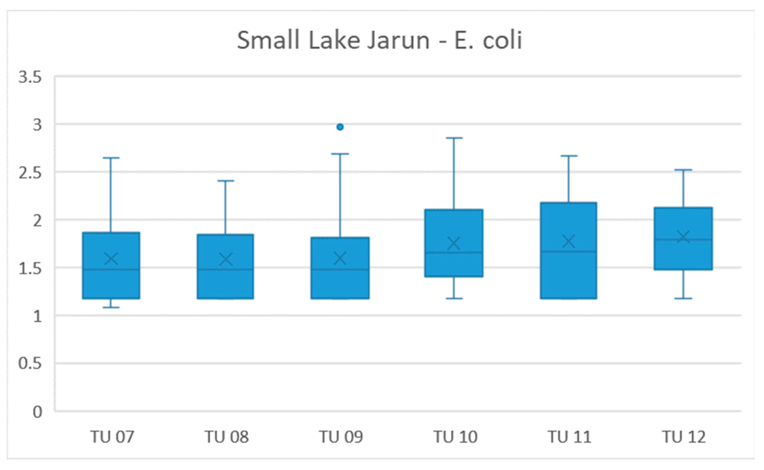
A comprehensive collection of 182 samples was obtained from six locations: TU 07 with 32 samples, TU 08, TU 09, TU 10, TU 11, and TU 12, each also containing 32 samples, at the Small Lake Jarun. The computed logarithmic values of the E. coli concentrations in Small Lake Jarun are illustrated using a box diagram in Figure 12.

Figure 12 illustrates the distribution of E. coli in the Small Lake Jarun, with the distribution interval ranging from 1.1 to 2.9. At sampling points TU 07, TU 08, and TU 10, the distribution is characterized by a rightward skew, while at other sampling points, it exhibits a symmetrical distribution. The average concentrations of E. coli vary between 1.588 (at the TU 08 location) and 1.817 (at the TU 12 location). In the sampling area at the TU 09 location, one data point is situated above the whisker, indicating an outlier, meaning a value that diverges from the other measurements. The calculation of the one-factor analysis of variance was conducted utilizing an Excel tool with a significance level of α = 0.05. This significance level denotes the threshold for deciding to reject the null hypothesis. The results of the analysis examining the relationship between the concentration of E. coli and sampling points across the defined locations are detailed in the ANOVA table, Table 3. As shown in Table 3, p = 0.005 < 0.05, indicating a statistically significant difference in mean concentrations among sampling locations. The final determination is made by comparing the value of the test statistic with the critical value of the test statistic. The value of the test statistic, 5.632, exceeds the value of the critical test statistic, 3.098; therefore, the null hypothesis of equal mean concentrations across sampling locations is rejected, indicating a statistically significant difference among sampling locations [29,30].

Table 3. Data presentation for Lake Bundek (E. coli).

Sources of Data Dispersion	Degrees of Freedom	Sum of Squares of Deviations	Corrected Variance	Value of the Test Statistic	p Value	Critical Value of the Test Statistic
Among the arrays	2	2.413	1.206	5.632	0.005	3.098
Random error	90	19.276	0.214
Total	92	21.688

Figure 12. Box-and-whisker plot of log₁₀-transformed E. coli concentrations (CFU/100 mL) at sampling locations TU7-TU12 on Small Lake Jarun (2016–2019).

Figure 12. Box-and-whisker plot of log₁₀-transformed E. coli concentrations (CFU/100 mL) at sampling locations TU7-TU12 on Small Lake Jarun (2016–2019).

For the Great Lake Jarun (Table 4), the p-values exceed the significance level (p > α), and therefore the null hypothesis of equal mean concentrations across sampling locations is not rejected. This indicates that no statistically significant differences in mean microbiological concentrations were detected among sampling locations. By additionally computing the value of the test statistic and the critical value of the test statistic, this presumption is validated.

Table 4. Data presentation for Great Lake Jarun (E. coli).

Sources of Data Dispersion	Degrees of Freedom	Sum of Squares of Deviations	Corrected Variance	Value of the Test Statistic	p Value	Critical Value of the Test Statistic
Among the arrays	5	0.439	0.088	0.436	0.823	2.263
Random error	184	37.080	0.202
Total	189	37.519

By conducting an analysis of the relationship between the amount of E. coli in the Small Lake Jarun (Table 5), and by comparing the values of test statistics against the critical value of test statistics, it becomes apparent that there exist no statistically significant differences among sampling points.

Table 5. Data presentation for Small Lake Jarun (E. coli).

Sources of Data Dispersion	Degrees of Freedom	Sum of Squares of Deviations	Corrected Variance	Value of the Test Statistic	p Value	Critical Value of the Test Statistic
Among the arrays	5	1.692	0.338	1.697	0.138	2.265
Random error	184	35.085	0.199
Total	189	36.777

The implementation of a one-factor analysis of variance enabled the identification of a potential statistically significant difference in mean E. coli concentrations among sampling locations during the study period. There is no statistically significant spatial difference in E. coli concentrations among sampling locations at Great and Small Lake Jarun, whereas a statistically significant spatial difference is observed at Lake Bundek.

The statistically significant spatial variability in E. coli observed at Lake Bundek may be related to its smaller size, higher water temperature, and higher bather density compared to Lake Jarun, which can enhance local bacterial growth and reduce dilution. However, these factors were not included as quantitative predictors in the statistical model and therefore should be interpreted as potential drivers rather than demonstrated causal mechanisms.

3.2.2. The Number of Intestinal Enterococci in Lakes Bundek and Jarun

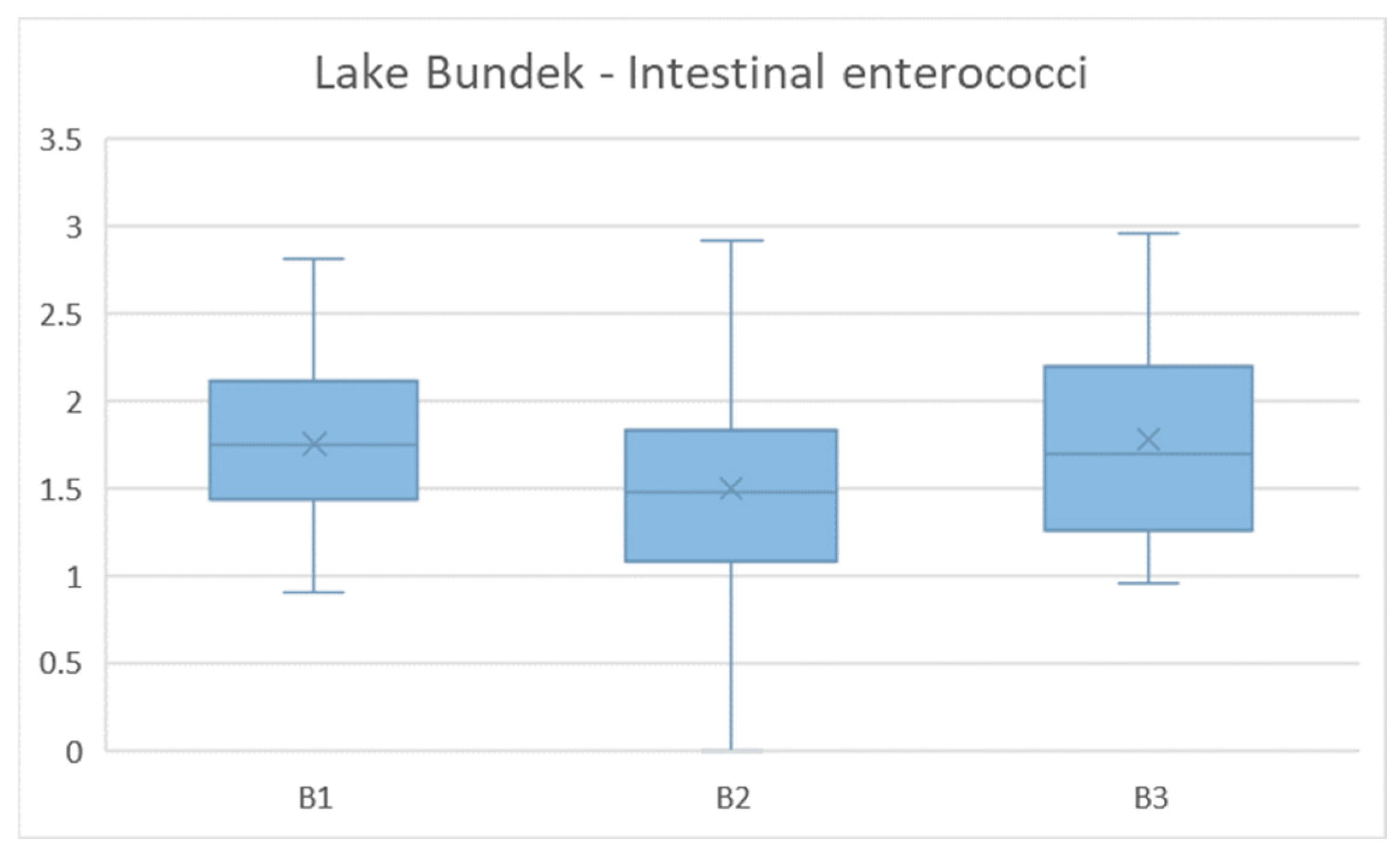
A total of 93 samples were collected at Lake Bundek from three locations: B1 from the eastern coast, B2 from the western coast, and B3 from the southern shore, specifically, 31 samples from each location. The computed logarithmic values of the quantity of intestinal enterococci present in Lake Bundek are presented in a box diagram in Figure 13.

Figure 13 illustrates the distribution of intestinal enterococci levels in Lake Bundek, where the largest distribution interval is evident on the western shore at point B2, ranging from 0.0 to 2.9. The highest recorded level of intestinal enterococci occurred on the southern coast at point B3, achieving a value of 3.00, while the maximum average level of 1.781 was noted at the same site. The distribution on the eastern and western coasts exhibits symmetry, whereas the southern coast displays a rightward slope. There are no outliers present for all three locations.

Figure 13. Box-and-whisker plot of log₁₀-transformed intestinal enterococci concentrations (CFU/100 mL) at sampling locations B1–B3 on Lake Bundek (2016–2019).

Figure 13. Box-and-whisker plot of log₁₀-transformed intestinal enterococci concentrations (CFU/100 mL) at sampling locations B1–B3 on Lake Bundek (2016–2019).

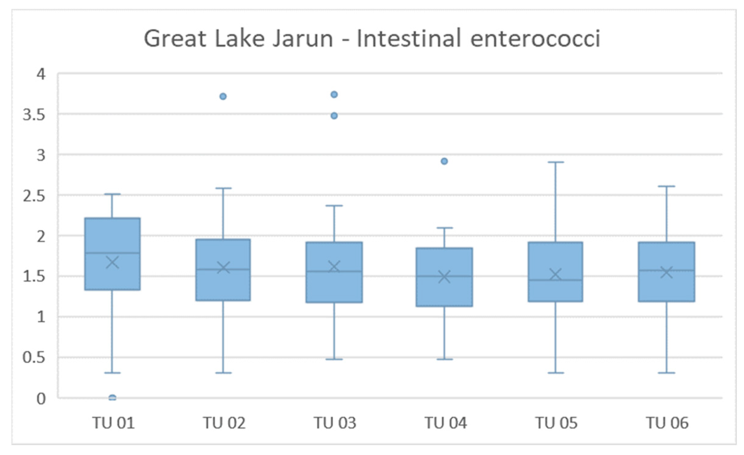
A total of 190 samples were collected from six locations: TU 01 with 30 samples, TU 02 with 32 samples, TU 03 with 34 samples, TU 04 with 32 samples, TU 05 with 32 samples, and TU 06 with 30 samples at the Great Lake Jarun. The computed logarithmic values of the quantity of intestinal enterococci present in the Great Lake Jarun are illustrated in a box diagram (Figure 14).

The maximum value of the quantity of intestinal enterococci on the Great Lake Jarun is observed at the location TU 05, where it registers a value of 2.9 (Figure 14). The average quantities of intestinal enterococci at points TU 01, TU 02, TU 03, TU 04, TU 05, and TU 06 range from 1.491 to 1.668. At the locations TU 01, TU 02, TU 03, and TU 04, there are dots appearing both above and below the whisker, indicating information that deviates from the others. The distribution of the data is symmetrical for the locations TU 01, TU 02, and TU 03, whereas for the locations TU 04 and TU 06, it is skewed to the left, and for TU 05, it is skewed to the right.

Figure 14. Box-and-whisker plot of log₁₀-transformed intestinal enterococci concentrations (CFU/100 mL) at sampling locations B1–B3 on Great Lake Jarun (2016–2019).

Figure 14. Box-and-whisker plot of log₁₀-transformed intestinal enterococci concentrations (CFU/100 mL) at sampling locations B1–B3 on Great Lake Jarun (2016–2019).

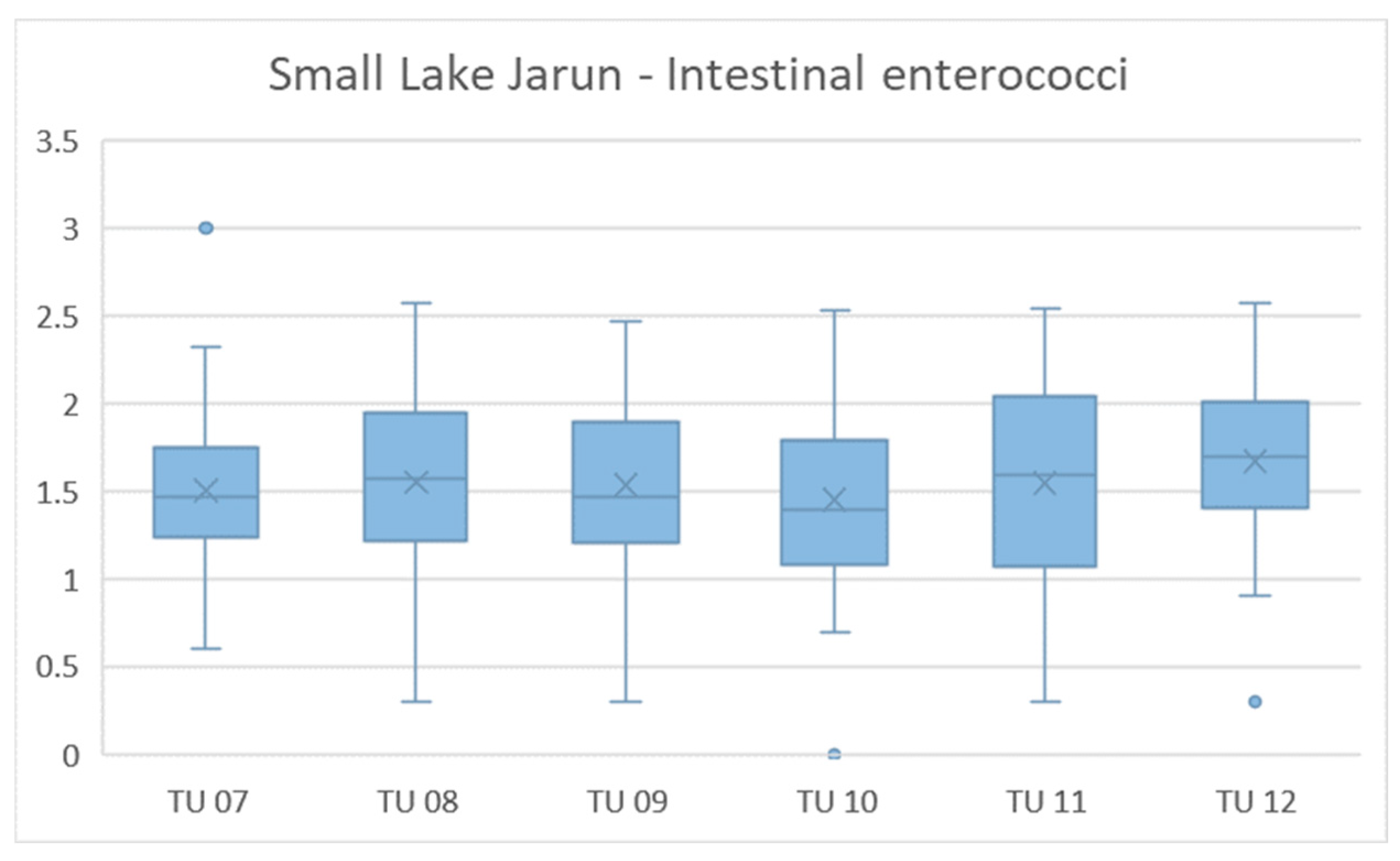
A total of 182 samples from six locations, specifically TU 07 with 32 samples, TU 08, TU 09, TU 10, TU 11, and TU 12 each with 32 samples, were taken at the Small Lake Jarun. The computed logarithmic values of the quantity of intestinal enterococci in the Small Lake Jarun are represented by a box diagram in Figure 15.

Figure 15 illustrates the distribution of intestinal enterococci in Small Lake Jarun, with the distribution interval ranging from 0.3 to 2.6. At the sites TU 07, TU 09, and TU 10, the distribution exhibits a rightward skew, while at sites TU 08 and TU 12 it appears symmetrical, and at site TU 11 it demonstrates a leftward skew. The average quantities of intestinal enterococci vary from 1.450 (at the TU 10 site) to 1.667 (at the TU 12 site). Within the vicinity of Small Lake Jarun, three points emerge that represent an outlier. The calculation of the analysis regarding the relationship between intestinal enterococci and sampling points for defined locations is presented in Table ANOVA, Table 6. From Table 6, the p-value is p = 0.124, which exceeds the significance level α (0.05), indicating that there is no statistically significant effect on the mean. The final determination is made by comparing the value of the test statistic to the critical value of the test statistic [15,16,17,18,19]. Because the p-value exceeds the significance level (p = 0.124 > 0.05) and the test statistic does not exceed the critical value (F = 2.134 < F_crit = 3.098), the null hypothesis of equal mean concentrations among sampling locations is not rejected.

Table 6. Data presentation for Lake Bundek (intestinal enterococci).

Sources of Data Dispersion	Degrees of Freedom	Sum of Squares of Deviations	Corrected Variance	Value of the Test Statistic	p Value	Critical Value of the Test Statistic
Among the arrays	2	1.459	0.730	2.134	0.124	3.098
Random error	90	30.774	0.342
Total	92	32.234

Figure 15. Box-and-whisker plot of log₁₀-transformed intestinal enterococci concentrations (CFU/100 mL) at sampling locations B1–B3 on Small Lake Jarun (2016–2019).

Figure 15. Box-and-whisker plot of log₁₀-transformed intestinal enterococci concentrations (CFU/100 mL) at sampling locations B1–B3 on Small Lake Jarun (2016–2019).

Although the graphical distributions suggest some variability among sampling locations at Great and Small Lake Jarun, the one-way ANOVA results (Table 4 and Table 5) show that these differences are not statistically significant. This indicates a spatially homogeneous distribution of E. coli within the Jarun system, consistent with a well-mixed water body and distributed contamination sources rather than localized hotspots.

For intestinal enterococci, the absence of statistically significant spatial differences at all lakes indicates a homogeneous spatial pattern, suggesting that contamination sources are diffuse and that hydrodynamic mixing dominates over localized inputs.

The interpretation of the data presented in Table 7 remains consistent with that of the preceding table (Table 6). Through a comparison of the values of the test statistics with the critical values of the test statistics, in accordance with statistical principles, it can be concluded that the values of the microbiological parameters from the samples are not influenced by the sampling location.

Table 7. Data presentation for Great Lake Jarun (intestinal enterococci).

Sources of Data Dispersion	Degrees of Freedom	Sum of Squares of Deviations	Corrected Variance	Value of the Test Statistic	p Value	Critical Value of the Test Statistic
Among the arrays	5	0.682	0.136	0.372	0.867	2.263
Random error	184	67.429	0.366
Total	189	68.111

Additionally, the same applies to Table 8. The critical value of the test statistics is less than the computed value of the test statistics, and in accordance with the stipulated guidelines, the assumption is accepted, meaning that the values of microbiological parameters from the samples are independent of the sampling location.

Table 8. Data presentation for Small Lake Jarun (intestinal enterococci).

Sources of Data Dispersion	Degrees of Freedom	Sum of Squares of Deviations	Corrected Variance	Value of the Test Statistic	p Value	Critical Value of the Test Statistic
Among the arrays	5	0.774	0.155	0.538	0.747	2.265
Random error	176	50.660	0.288
Total	181	51.435

Across the study period (2016–2019), one-way ANOVA showed no statistically significant spatial differences in intestinal enterococci among sampling locations at Lake Bundek, Great Lake Jarun, or Small Lake Jarun (Table 6, Table 7 and Table 8, p ≥ 0.05).

This spatial homogeneity suggests that enterococci are relatively well distributed within each lake, which may reflect effective hydrodynamic mixing and/or diffuse contamination inputs rather than persistent, localized hotspots. Short-term drivers such as rainfall, temperature, and variations in bather load may influence overall concentrations over time. However, because these variables were not included as quantitative predictors in the statistical model, they are discussed here only as probable influences rather than demonstrated causal mechanisms. Specifically, at all sites (Bundek, Small, and Great Lake Jarun), there is an absence of statistical connection between the arithmetic mean of the quantity of intestinal enterococci and the sampling locations.

The absence of statistically significant spatial differences in intestinal enterococci across all sites (Bundek, Great Jarun, and Small Jarun) indicates a largely homogeneous spatial distribution, which is consistent with efficient water mixing, diffuse contamination sources, and the lack of persistent local pollution hotspots. Short-term meteorological effects such as rainfall and temperature may influence overall bacterial levels, but they do not generate stable spatial gradients between sampling locations. Rainfall events can intermittently increase microbial loads via runoff and resuspension, whereas temperature and solar radiation affect survival and persistence of fecal indicator bacteria; such effects primarily contribute to temporal variability rather than stable spatial gradients in well-circulated systems.

4. Conclusions

This study evaluated spatial variability in Escherichia coli and intestinal enterococci in two urban recreational lakes in Zagreb (Bundek and Jarun) using four years (2016–2019) of routine bathing water monitoring data. Log₁₀-transformed microbiological concentrations were analyzed using one-way ANOVA, with variability visualized through box-and-whisker plots, which are appropriate for skewed MPN and CFU-based data.

The results indicate predominantly spatially homogeneous distributions of microbiological indicators, particularly at Lake Jarun, where no statistically significant differences among sampling locations were detected. In contrast, a statistically significant spatial difference in E. coli concentrations was observed at Lake Bundek, likely reflecting site-specific characteristics such as smaller lake size and more limited water exchange. These factors were not explicitly modelled and are therefore interpreted as potential influences.

Overall, the findings indicate that routine bathing-water monitoring at multiple fixed locations captures essential information on microbiological water quality, while also suggesting that, in well-mixed systems, monitoring optimisation may be feasible without compromising public health protection. Continuous surveillance remains essential to ensure safe recreational use of urban lakes and to enable timely management responses when elevated microbiological levels occur.

References

- Freshwater Crisis. National Geographic. Available online: https://www.nationalgeographic.com/environment/freshwater/freshwater-crisis/ (accessed on 20 September 2025).
- Boelee, E.; Geerling, G.; van der Zaan, B.; Blauw, A.; Vethaak, A.D. Water and health: From environmental pressures to integrated responses. Acta. Trop. 2019, 193, 217–226. [Google Scholar] [CrossRef] [Scilit] [PubMed]
- Gomes, L.; Bordalo, A.A.; Machado, A. Characterization of Escherichia coli Isolates in Recreational Waters: Implications for Public Health and One Health Approach. Water 2024, 16, 2925. [Google Scholar] [CrossRef] [Scilit]
- Directive 2006/7/EC of the European Parliament and of the Council of 15 February 2006 Concerning the Management of Bathing Water Quality and Repealing Directive 76/160/EEC. Available online: https://eur-lex.europa.eu/eli/dir/2006/7/oj/eng (accessed on 7 January 2026).
- Dimpor, J.J.; Lucky, O.P.; Kwarkye, D.F.; Watts, S.; Oguayo, C.P.; Ojewole, C.O.; Kusi, J. Identifying spatiotemporal patterns and drivers of fecal indicator bacteria in an urban lake for water quality assessment and management. Heliyon 2025, 11, e40955. [Google Scholar] [CrossRef] [Scilit] [PubMed]
- van der Meulen, E.S.; Tertienko, A.; Blauw, A.N.; Sutton, N.B.; van de Ven, F.H.M.; Rijnaarts, H.H.M.; Oel, P.R. A review of prediction models for E. coli in urban surface waters. Urban Water J. 2024, 21, 539–548. [Google Scholar] [CrossRef] [Scilit]
- Yoneda, I.; Nishiyama, M.; Watanabe, T. Comparative experiment to select water quality parameters for modelling the survival of Escherichia coli in lakes. Environ. Pollut. 2024, 357, 124423. [Google Scholar] [CrossRef] [Scilit] [PubMed]
- Jozić, S.; Cenov, A.; Glad, M.; Peroš-Pucar, D.; Kurić, K.; Puljak, T.; Ordulj, M.; Vrdoljak Tomaš, A.; Baumgartner, N.; Ivanković, D.; et al. The effect of sampling frequency and spatial and temporal variation in the density of fecal indicator bacteria on the assessment of coastal bathing water quality. Water Res. 2024, 264, 122192. [Google Scholar] [CrossRef] [Scilit] [PubMed]
- Quero, G.M.; Guicciardi, S.; Penna, P.; Catenacci, G.; Brandinelli, M.; Bolognini, L.; Luna, G.M. Increasing trends in faecal pollution revealed over a decade in the central Adriatic Sea (Italy). Water Res. 2024, 262, 122083. [Google Scholar] [CrossRef] [Scilit] [PubMed]
- Heasley, C.; Sanchez, J.J.; Tustin, J.; Young, I. Systematic review of predictive models of microbial water quality at freshwater recreational beaches. PLoS ONE 2016, 16, e0256785. [Google Scholar] [CrossRef] [Scilit] [PubMed]
- Rose, J.B.; Hofstra, N.; Hollmann, E.; Katsivelis, P.; Medema, G.J.; Murphy, H.M.; Naughton, C.C.; Verbyla, M.E. Global microbial water quality data and predictive analytics: Key to health and meeting SDG 6. PLoS Water 2023, 2, e0000166. [Google Scholar] [CrossRef] [Scilit]
- Manini, E.; Baldrighi, E.; Ricci, F.; Grilli, F.; Giovannelli, D.; Intoccia, M.; Casabianca, S.; Capellacci, S.; Marinchel, N.; Penna, P.; et al. Assessment of Spatio-Temporal Variability of Faecal Pollution along Coastal Waters during and after Rainfall Events. Water 2022, 14, 502. [Google Scholar] [CrossRef] [Scilit]
- World Health Organization (WHO). Guidelines on Recreational Water Quality: Volume 1 Coastal and Fresh Waters. Available online: https://www.who.int/publications/i/item/9789240031302 (accessed on 7 January 2026).
- Federigi, I.; Bonadonna, L.; Bonanno Ferraro, G.; Briancesco, R.; Cioni, L.; Coccia, A.M.; Carducci, A. Quantitative microbial risk assessment as support for bathing waters profiling. Mar. Pollut. Bull. 2020, 157, 111319. [Google Scholar] [CrossRef] [Scilit]
- Seis, W.; Ten Veldhuis, M.C.T.; Rouault, P.; Steffelbauer, D.; Medema, G. A new Bayesian approach for managing bathing water quality at river bathing locations vulnerable to short-term pollution. Water Res. 2024, 252, 121186. [Google Scholar] [CrossRef] [Scilit] [PubMed]
- Adhikary, R.K.; Starrs, D.; Wright, D.; Croke, B.; Glass, K.; Lal, A. Spatio-Temporal Variation in the Exceedance of Enterococci in Lake Burley Griffin: An Analysis of 16 Years’ Recreational Water Quality Monitoring Data. Int. J. Environ. Res. Public Health 2024, 21, 579. [Google Scholar] [CrossRef] [Scilit] [PubMed]
- Durham, B.W.; Porter, L.; Webb, A.; Thomas, J. Seasonal influence of environmental variables and artificial aeration on Escherichia coli in small urban lakes. J. Water Health 2016, 14, 929–941. [Google Scholar] [CrossRef] [Scilit] [PubMed]
- Palmer, J.A.; Law, J.Y.; Soupir, M.L. Spatial and temporal distribution of E. coli contamination on three inland lake and recreational beach systems in the upper Midwestern United States. Sci. Total Environ. 2020, 722, 137846. [Google Scholar] [CrossRef] [Scilit] [PubMed]
- Zagreb Danas, Bundek Gradski Park i Jezero. Available online: https://www.zgportal.com/o-zagrebu/povijest-zagrebackih-naselja/bundek/ (accessed on 20 September 2025).
- Kratka Povijest Zagrebačkog Jezera Jarun. Available online: https://kurziv.net/kratka-povijest-zagrebackog-jezera-jarun/ (accessed on 10 January 2026).
- Bathing Water Quality Regulation (NN 51/14). Available online: https://narodne-novine.nn.hr/clanci/sluzbeni/2014_04_51_978.html (accessed on 20 September 2025).
- EPA. Recreational Water Quality Criteria. Available online: https://www.epa.gov/sites/production/files/2015-10/documents/rwqc2012.pdf (accessed on 20 September 2025).
- HRN EN ISO 9308-3:2000; Water Quality-Detection Numeration of Escherichia coli Coliform Bacteria in Surface Waste Water Part 3 Miniature Method (Most Likely Number Method) for Detection Counting of, E. coli in Surface and Waste Water. European Committee for Standardization (CEN): Brussels, Belgium, 2000.
- HRN EN ISO 7899_2: 2000; Water Quality-Detection and Enumeration of Intestinal Enterococci-Part 2: Membrane Filtration Method. ISO: Geneva, Switzerland, 2000.
- Zar, Z.H. Biostatistical Analysis; Printice Hall Inc.: Englewood Clifs, NJ, USA, 1999; pp. 592–663. [Google Scholar]
- Hoffman, J.I.E. (Ed.) Analysis of Variance I. One-Way. In Biostatistics for Medical and Biomedical Practitioners; Academic Press: Cambridge, MA, USA, 2015; pp. 391–420. [Google Scholar]
- Hassan, A.; Samy, G.; Hegazy, M.; Balah, A.; Fathy, S. Statistical analysis for water quality data using ANOVA (Case study–Lake Burullus influent drains). Ain. Shams Eng. J. 2024, 15, 102652. [Google Scholar] [CrossRef] [Scilit]
- Pujar, P.M.; Kenchannavar, H.H.; Kulkarni, R.M.; Kulkarni, U.P. Real-time water quality monitoring through Internet of Things and ANOVA-based analysis: A case study on river Krishna. Appl. Water Sci. 2020, 10, 22. [Google Scholar] [CrossRef] [Scilit]
- Thomas, E.O. Evaluation of groundwater quality using multivariate, parametric and non-parametric statistics, and GWQI in Ibadan, Nigeria. Water Sci. 2023, 37, 117–130. [Google Scholar] [CrossRef] [Scilit]
- Berkowitz, M.; Altman, R.; Loughin, T. Random forests for survival data: Which methods work best and under what conditions? Int. J. Biostat. 2024, 20, 315–345. [Google Scholar] [CrossRef] [Scilit] [PubMed]
Disclaimer/Publisher’s Note: The statements, opinions and data contained in all publications are solely those of the individual author(s) and contributor(s) and not of MDPI and/or the editor(s). MDPI and/or the editor(s) disclaim responsibility for any injury to people or property resulting from any ideas, methods, instructions or products referred to in the content. |
© 2026 by the authors. Licensee MDPI, Basel, Switzerland. This article is an open access article distributed under the terms and conditions of the Creative Commons Attribution (CC BY) license.