An Integrated Geophysical Investigation of the Flavia Seamount in the Northern Tyrrhenian Back-Arc Basin (Mediterranean Sea)

Abstract

Despite its geodynamic significance, the northern Tyrrhenian Back-Arc Basin, characterized by a complex tectono-magmatic evolution, remains poorly investigated. We present the first geophysical characterization of the Flavia Seamount, a previously uninvestigated edifice in the northern Tyrrhenian Sea, integrating new multibeam, seismic, and magnetic data. The new high-resolution bathymetric data reveal a flat, nearly circular summit and strongly asymmetric flanks. Reduced-to-the-pole magnetic anomalies exhibit a north–south polarity pattern, with positive values in the northern sector and negative values in the southern sector. Seismic data, integrated with Sparker profiles collected in 1985, reveal a flat-topped acoustic basement overlain by a ~100 m thick stratified sequence and affected by inactive east-dipping extensional faults, indicating tectonic control on the evolution of the seamount. Widespread landslide scarps and associated mass-transport deposits document recurrent gravitational instability along the flanks and within surrounding basins. Pockmark morphometry suggests distinct formation processes, with summit pockmarks controlled by fluid seepage and gravitational processes, and basin pockmarks mainly related to fluid escape from mass-transport deposits. Magnetic forward modelling constrained by seismic data provides new insights into the distribution of magnetic susceptibility bodies and the crustal architecture beneath the seamount. Results suggest that the present-day morphology of the Flavia Seamount reflects the combined effects of tectonic, sedimentary, and gravitational processes.

1. Introduction

Back-arc basins (BABs) record the coupled action of crustal extension, magmatism, and mantle flow within a geodynamic setting that remains fundamentally linked to subduction [1,2,3]. Their development is commonly associated with deep mantle drag forces that promote extension in the overriding plate, upper- and middle-crustal stretching, faulting, seafloor spreading, and volcanism. At the same time, mantle circulation and magma ascent may enhance extension and promote mechanical decoupling within the extending lithosphere, thereby influencing both the architecture and the magma activity of the basins and the surrounding volcanic arc regions [4,5,6,7].

The marginal domains of BABs are especially complex because they are not simple passive edges of extension, but transitional zones inheriting the crustal structure, variable rheology and magmatism. In fact, along the BAB edges, changing plate kinematics interact to produce intense faulting, block rotation, uplift, basin asymmetry, and strain partitioning. For this reason, understanding the tectonic deformation along the boundaries of back-arc basins remains one of the most challenging problems in subduction-zone tectonics [8,9].

The Tyrrhenian Sea, located in the central Mediterranean region, is a remarkable example of a BAB developed within a compressional framework, where an oceanic plate is subducted beneath continental lithosphere [10,11,12,13,14,15,16]. The opening of the northern sector of the Tyrrhenian BAB began during the Late Tortonian [17,18], making it the oldest portion of the basin.

The morphology of the northern Tyrrhenian BAB is characterized by a series of N–S-trending seamounts and elongated basins [19,20,21], interpreted as half-graben and graben–horst systems associated with extensional tectonics, magmatic intrusions, and alkaline volcanism [12,17,22,23]. Several of these bathymetric highs (e.g., the Cialdi, Etruschi, Tiberino and Vercelli) are documented in existing atlases of the Tyrrhenian seamounts [24,25] and in [26]. However, despite the key role of the northern Tyrrhenian domain for reconstructing the geodynamic evolution of the basin and its surrounding margins, this region has received comparatively less scientific attention than the southern Tyrrhenian region. As a result, several morphological features remain poorly constrained and only tentatively interpreted, largely because of the limited availability of geological and geophysical data.

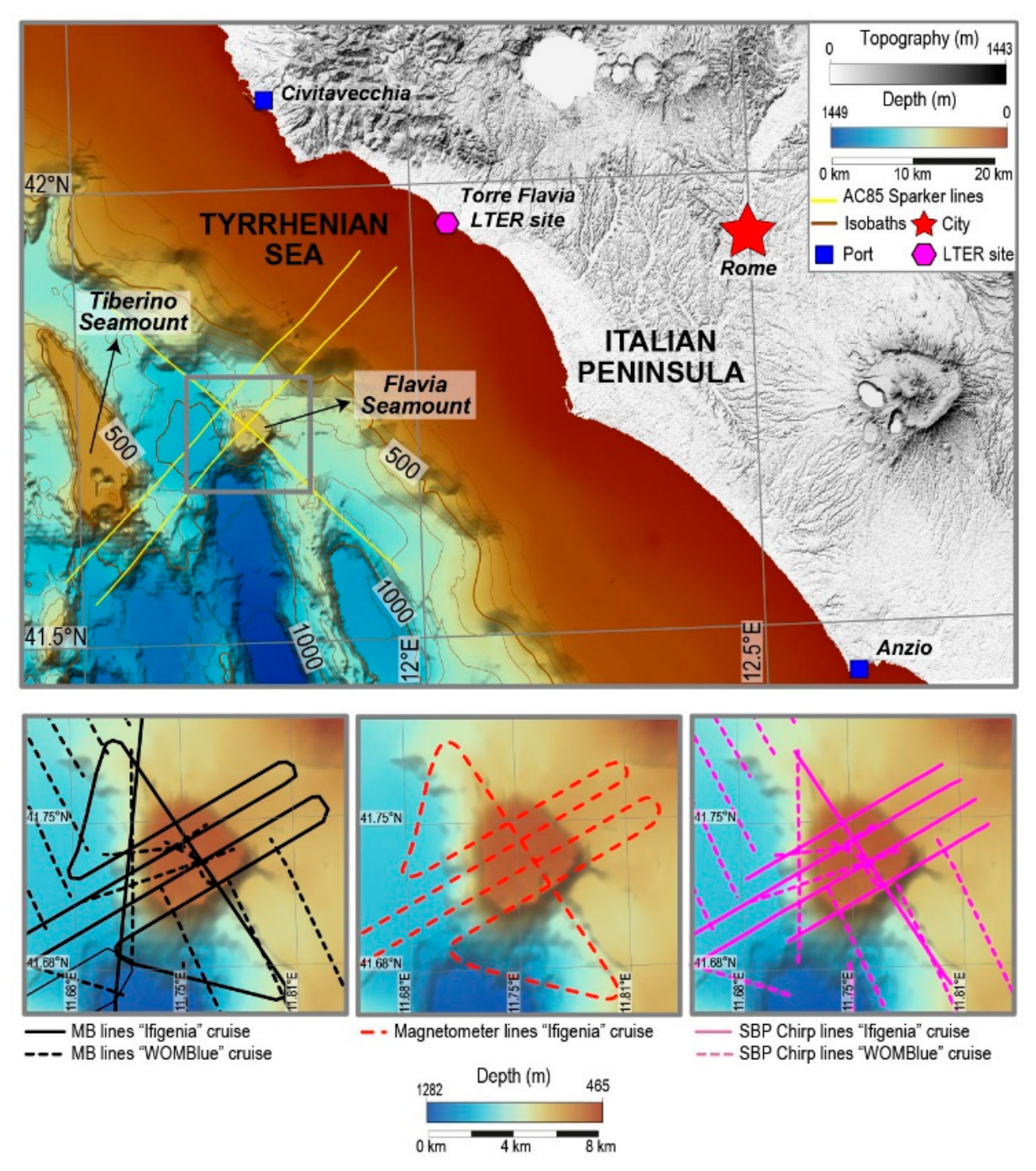
Among these features, a prominent morphological high stands out for its nearly circular shape, in contrast to the more elongated N–S-oriented structures typical of the region. This feature is located approximately 35 km off the western coast of the Italian Peninsula and ~12 km east of the Tiberino Seamount (Figure 1). Following the Latin-based nomenclature traditionally adopted for the Tyrrhenian seamounts [24,25], this feature is hereafter referred to as the “Flavia Seamount”, named in tribute to the “Torre Flavia” Italian Long-Term Ecological Research (LTER-Italy) site [27], located along the Italian coastline at approximately the same latitude as Rome (Figure 1). To better constrain the Flavia Seamount (hereafter referred to as FS) and to improve the geodynamic understanding of the area, new bathymetric, magnetic, and seismic datasets were acquired during two oceanographic cruises conducted aboard the National Research Council (CNR) R/V Gaia Blu (“Ifigenia” [28] and “WOMBlue” [29]). Prior to these cruises, the available data for this region consisted of several Sparker seismic profiles (30 kJ) collected in 1985 [30], along with bathymetric and magnetic measurements collected during the TIR99 survey in 1999 [31], an oceanographic cruise finalized to produce the first high-resolution bathymetric mapping of the Tyrrhenian BAB. Unfortunately, the bathymetric data collected during this campaign covered only the western sector of the FS. Consequently, the morphological description of this prominent high was performed by integrating TIR99 data and satellite-derived bathymetry (Figure 1).

In this work, we present, for the first time, high-resolution bathymetric and magnetic maps of the entire extent of FS. The new bathymetric dataset enabled a detailed geomorphological analysis, leading to the identification of the main morpho-structural lineaments and numerous circular depressions interpreted as pockmarks, both on the summit of the seamount and within the basin located to the east side of FS. Each pockmark was individually mapped and catalogued, recording the geographic coordinates of its centre, water depth, internal depth, perimeter and area. Results of this morphometric analysis are summarized in two tables and illustrated through statistical plots.

In addition, high-resolution seismic profiles acquired using a Sub-Bottom Profiler Chirp during the Ifigenia and WOMBlue surveys, together with selected Sparker 30 kJ profiles acquired by the CNR in 1985 (yellow lines shown in Figure 1), were interpreted. While Sub-Bottom Profiler data show sedimentary structures within the upper ~40 m below the seafloor and provide insights into recent sedimentary processes and neotectonic deformation, the deeper-penetrating Sparker profiles allow reconstruction of the top of the acoustic basement, thereby constraining the morphotectonic framework of the seamount.

Finally, based on the newly acquired bathymetric and magnetic datasets together with the interpretation of Sparker seismic profiles, two geophysical models were developed to estimate the magnetic signature of the FS basement. The integrated analysis of these complementary geophysical datasets provided stronger constraints on the geological nature and origin of the basement than could be achieved using any single dataset alone.

2. Materials and Methods

2.1. Bathymetry

The middle-resolution (115 × 115 m) bathymetric data used to create Figure 1 was derived from EMODnet [32].

The new high-resolution (20 × 20 m) bathymetric map of the FS presented in this paper results from the acquisition of two datasets obtained during the Ifigenia [28] and WOMBlue [29] oceanographic cruises (see the bottom left inset in Figure 1). Two different multibeam echosounder (MBES) systems, hull-mounted on the vessel keel in a T configuration of linear transducer arrays, were used: the Kongsberg EM712 (1° × 0.5°), which operates dynamically across a frequency range of 40–100 kHz and is suitable for water depths between 150 and 1000 m; and the Kongsberg EM304 MKII (1° × 1°), operating at 30 kHz for depths exceeding 1000 m. A Valeport Mini Sound Velocity Sensor (SVS) continuously measured the sound velocity adjacent to the transducers to optimize beam-forming. In addition, sound velocity profiles were systematically collected throughout the cruises [28,29] using a Valeport MIDAS Sound Velocity Profiler (SVP). These profiles were used to correct depth measurements for variations in water-column stratification and acoustic velocity, thereby minimizing refraction-induced errors and improving the vertical and horizontal accuracy of the bathymetric data. Ship positioning was provided by the Seapath 380 system, utilizing a Fugro HP Differential Global Positioning System (DGPS) with Marinestar GNSS corrections, providing positioning accuracy better than 5 cm. The Kongsberg MRU 5 (Motion Reference Unit) and the dual-antenna GPS integrated into the Seapath system were used to correct for vessel pitch, roll, heave, and yaw, achieving accuracies of 0.02° for roll and pitch and 0.075° for heading. Data were acquired in the WGS84/UTM Zone 32N coordinate reference system.

The multibeam data were processed using QPS Qimera [35]. A standard workflow was applied, which first involved correcting for tidal variations to account for vertical changes in water level. Information on local tides (from the tide gauges at Civitavecchia and Anzio; Figure 1) was retrieved from the National Tide Gauge Network [36]. Sound speed corrections were then applied to correct for acoustic ray refraction and ensure the accuracy of the seabed mapping.

The dataset was further refined through a combination of automatic and manual filtering to remove spurious readings and noise.

The processed data were used to generate a final bathymetric surface with a grid resolution of 20 m, which was exported as an ArcView grid. The morphological and tectonic features were subsequently interpreted and digitized using Global Mapper [33] to produce the 2D digital elevation maps presented in this study.

2.2. Magnetic Data and Modelling

Magnetic data were collected during the Ifigenia cruise (see the bottom central inset in Figure 1) using an overhauser SeaSpy Marine Magnetics equipped with 300 m of electromechanical cable. The magnetometer was towed 240 m astern of the R/V Gaia Blu to reduce the noise produced by the vessel. Magnetic data were acquired at a nominal 1 Hz sampling rate and transmitted in near real-time onboard, where they were merged with standard navigation and communication of GPS satellite data NMEA0183 for geographical referencing. Towfish positioning was estimated by means of the lay-back computation.

Raw data have been corrected for spikes and diurnal variations using data from the INTERMAGNET reference station (INGV—Duronia magnetic observatory, IAGA [37]). Total intensity magnetic anomalies have been calculated by subtracting the International Geomagnetic Reference Field (IGRF) model [38] from the total field and then reduced to the pole (RTP) by FFT-phase shifting, using the local inclination and declination values of Earth’s magnetic field.

An interpretative reconstruction of the crustal structure beneath the FS region was obtained using 2.5D forward magnetic modelling based on the algorithms of [39,40]. The approach consists of defining a set of plausible causative sources and iteratively refining their geometries and magnetic susceptibility values by minimizing the misfit between the observed magnetic anomaly and the synthetic response generated by the modelled crustal structure. Because of the inherent non-uniqueness of potential-field data, the reliability of the resulting model is improved by incorporating independent constraints, particularly the available seismic information.

In the specific case, the modelling of FS was performed by sampling the magnetic anomaly field along the same tracks of Sparker 30 kJ profiles (AC85-17 and AC85-76) and constraining the geometries of the causative magnetic sources using depth-migrated seismic sections. Time-to-depth conversion of the seismic lines was performed using average seismic velocity values for three main layers: the water column (1500 m/s), Quaternary marine sediments (2100 m/s), and the basement layer (2500 m/s). Although this represents a simplified approach compared with the use of a detailed velocity profile, the resulting depth uncertainties can be considered acceptable in view of the resolution and overall accuracy of the forward magnetic modelling, particularly at greater depths. The modelling workflow consisted of evaluating the magnetic contribution of the stratified units recognized within the seismic sections and assigning starting susceptibility values based on literature data [26]. Furthermore, the best-fit procedure enables the determination of detailed magnetic properties of crustal bodies and inference of intervening causative bodies lacking a clear seismic signature, especially within the upper portion of the basement sequence. Additionally, the geometries of magnetic causative blocks implemented in the 2.5D modeling were constrained using symmetric and independent across-profile extensions.

2.3. Seismics

2.3.1. Sub-Bottom Profiler

Sub-Bottom Profiler (SBP) data were collected to provide high-resolution seismic and seismostratigraphic information on the upper ~40 m of the sedimentary succession. A keel-mounted Knudsen Chirp 3260 echosounder, equipped with a 3.5 kHz transducer array arranged in a 3 × 3 configuration, was used for this purpose. A Kongsberg K-Synk synchronization unit was employed during data acquisition to prevent acoustic interference between the Multibeam and the SBP systems. During the Ifigenia survey, high-resolution seismic profiles were collected following the survey layout planned for magnetometric investigation; additional data were acquired during the WOMBlue cruise to gather further information in areas not covered by previous investigations (see the bottom right inset in Figure 1).

SBP profiles were acquired in both KEB internal (i.e., binary, full-resolution envelope data) and filtered SEG-Y formats. A standard processing sequence (water-layer muting, low-pass filtering, and the application of linear gain) was carried out using Seaview [41] to improve the resolution and overall quality of the seismic images. Finally, a time-to-depth conversion was performed, assuming a nominal sound velocity of 1500 m/s for two-way travel time in both the water layer and the sedimentary cover. Processed data were then exported in SEG-Y format and imported into a 2D seismic interpretation software package (Kingdom 2024, S&P Global, Houston, TX, USA; [42]).

2.3.2. Sparker 30 kJ

The Sparker profiles used in this study are part of a legacy dataset collected, since the early 1970s, by the former Institute of Marine Geology (IGM)—now Institute of Marine Science (ISMAR)—of CNR, with the aim of studying the relationships between tectonics, magmatism and sedimentation along the Italian continental margins and the surrounding deep-sea basins. These seismic reflection profiles were acquired using a Sparker-type source (30 kJ, 1 kJ and 0.2 kJ) and recorded on paper. More recently, in line with the FAIR (Findable, Accessible, Interoperable, and Reusable) principles [43], a restoration and preservation initiative was undertaken to convert the paper records into georeferenced digital seismic sections ([44] and references therein). The resulting dataset is now integrated into the CNR-ISMAR Marine Spatial Data Infrastructure and is freely accessible upon request.

Here we present and discuss parts of three seismic profiles, acquired during the AC85 oceanographic cruise along the eastern Tyrrhenian continental margin, between Monte Argentario and Capo Circeo (the complete AC85 dataset is in [30]). These data were collected using a Sparker 30 kJ as a seismic source. Shot interval was set at 25 m, with a record length of 4 s two-way travel time (TWT).

3. Results

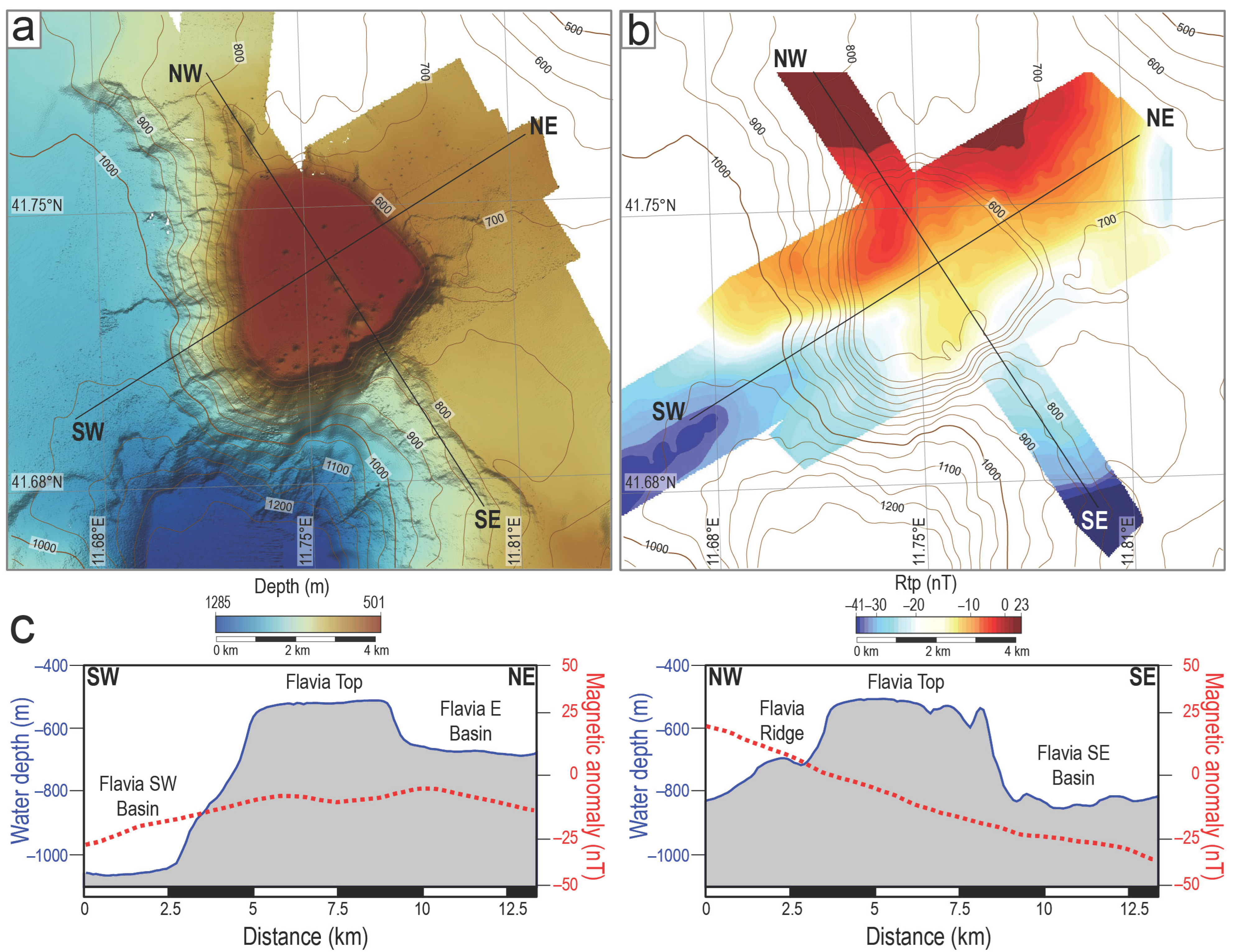
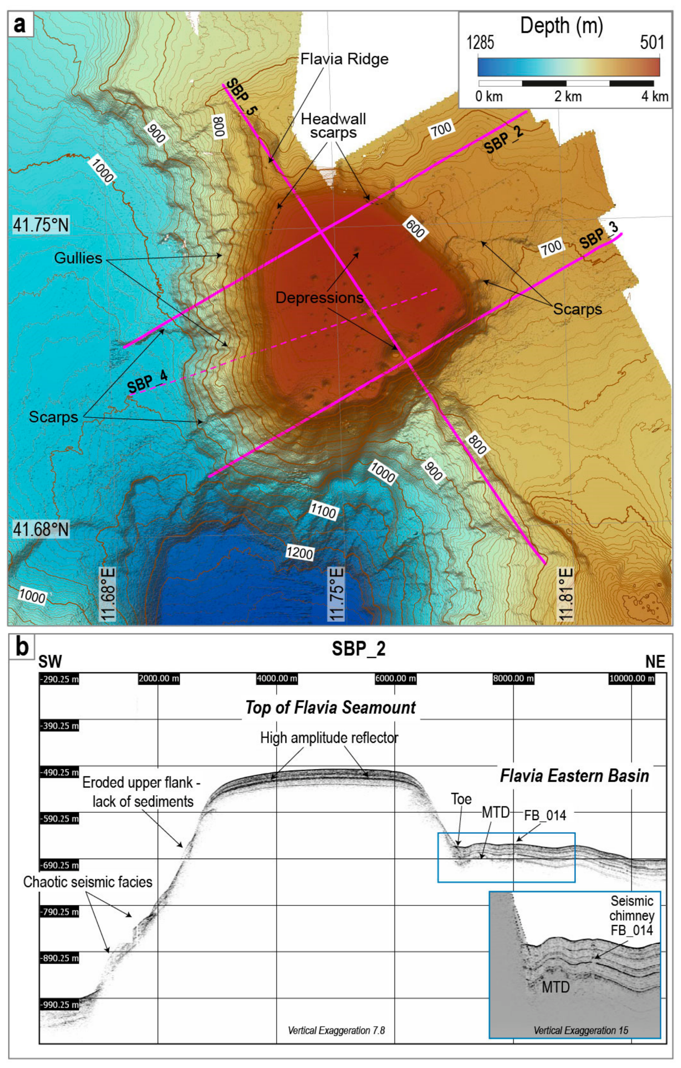
Bathymetric data (contour interval of 50 m) and RTP magnetic anomaly maps of the FS are presented in Figure 2a and Figure 2b, respectively. The main morphological features identified on the high-resolution bathymetric map (contour interval of 10 m), together with the interpreted SBP profiles, are shown in Figure 3. The distribution of pockmarks is illustrated on the slope-shaded bathymetric map (Figure 4), together with the methodology adopted to quantify their morphometric parameters. The results of the morphometric analysis, based on a statistical evaluation of the parameters reported in Supplementary Tables S1 and S2, are presented in Figure 5.

Furthermore, the three Sparker seismic profiles are presented and interpreted in Figure 6, while the original (uninterpreted) profiles are provided in Figure S1. Finally, two 2.5D forward magnetic models, constructed along selected segments of Sparker profiles AC85-17 and AC85-76, are shown in Figure 7.

3.1. Bathymetry and Magnetics

The bathymetry of the FS area (Figure 2a) is characterized by water depths ranging from ~500 to ~1300 m below sea level (b.s.l.). The shallowest depths occur at the summit of the FS, whereas the greatest depths are found within the basin located south of the FS.

The distribution of magnetic anomalies on the RTP map (Figure 2b) ranges from minimum values of approximately −41 nT, recorded in the southwestern and southeastern sectors of the study area, to positive values reaching up to 23 nT north of the FS. This pattern resembles the regional trend without any evidence of high-frequency, shallow crustal intervening sources.

The FS is characterized by a flat summit located at approximately 500 m b.s.l., gently dipping westward, as highlighted by the SW–NE bathymetric profile in Figure 2c. The summit area displays a nearly circular shape: considering the 550 m isobath as a reference, the seamount has a perimeter of approximately 17 km and a surface area of about 14.9 km².

Figure 2. Bathymetry and RTP magnetic anomaly maps of the FS area. Both panels were generated using Global Mapper software [33] in the UTM Zone 32N coordinate system (WGS84). Brown contour lines represent isobaths (contour interval at 50 m). (a) Shaded-relief image of multibeam bathymetry acquired during the CNR oceanographic cruises Ifigenia [28] and WOMBlue [29]. The bathymetric datasets were merged to produce a single 2D digital elevation model. Illumination parameters: sun elevation 70°, azimuth 330°, vertical exaggeration × 10. The color palette used is “Roma” [34]. Black lines indicate the location of the profiles shown below. (b) Shaded-relief map showing the distribution of RTP magnetic anomalies across the study area. (c) SW–NE- and NW–SE-oriented bathymetric and magnetic profiles. The grey fields indicate the seafloor morphology.

Figure 2. Bathymetry and RTP magnetic anomaly maps of the FS area. Both panels were generated using Global Mapper software [33] in the UTM Zone 32N coordinate system (WGS84). Brown contour lines represent isobaths (contour interval at 50 m). (a) Shaded-relief image of multibeam bathymetry acquired during the CNR oceanographic cruises Ifigenia [28] and WOMBlue [29]. The bathymetric datasets were merged to produce a single 2D digital elevation model. Illumination parameters: sun elevation 70°, azimuth 330°, vertical exaggeration × 10. The color palette used is “Roma” [34]. Black lines indicate the location of the profiles shown below. (b) Shaded-relief map showing the distribution of RTP magnetic anomalies across the study area. (c) SW–NE- and NW–SE-oriented bathymetric and magnetic profiles. The grey fields indicate the seafloor morphology.

The seamount exhibits a markedly asymmetric SW–NE profile (Figure 2c). The western flank, with an average slope of ~21% (Figure 2, Figure 3 and Figure 4a), extends from a depth of ~550 m to more than 1000 m within the adjacent southwestern basin, corresponding to a vertical relief of approximately 500 m. In contrast, the eastern flank, although slightly steeper (~23%; Figure 2, Figure 3 and Figure 4a), is significantly shorter, extending for only ~200 m, from a minimum of ~500 m to a maximum depth of ~700 m b.s.l. (Figure 2c). Along this profile, magnetic anomalies are predominantly negative (Figure 2c).

The NW–SE-oriented bathymetric profile (Figure 2c) provides further insights into its morphology and magnetic signature. In its northern sector, the profile intersects a morphological ridge, hereafter referred to as the Flavia Ridge (Figure 2c and Figure 3), along which the highest positive magnetic anomaly values of the study area are recorded. The central portion of the NW–SE-oriented profile reveals a more irregular summit morphology, where two distinct depressions can be identified near the southern flank. This profile is also markedly asymmetric: the northern flank has a slope of ~26% (Figure 2, Figure 3 and Figure 4a) and a vertical relief of approximately 200 m (from ~550 m to ~750 m depth), whereas the southern flank, which represents the steepest sector of the seamount (~33%; Figure 2, Figure 3 and Figure 4a), shows a vertical relief of about 300 m (from ~550 m to ~850 m depth). Magnetic anomaly values along this profile decrease progressively southward, approaching zero in the central sector and becoming negative (down to ~−40 nT) in the southern portion.

3.2. Morphology and Sub-Bottom Profiler

Geomorphic features (e.g., gullies, landslide scarps and deposits, and ridges) have been identified and highlighted with black arrows on the high-resolution bathymetric map (contour interval of 10 m) and on the SBP profiles shown in Figure 3a.

The SBP_2 profile (Figure 3b), SW–NE oriented, crosses the FS and reveals a western flank characterized by an eroded upper slope and the presence of chaotic seismic facies at the toe of the slope. The top of the FS is characterized by well-defined sub-parallel stratification, with a thickness of approximately 40 m. An interval of high-amplitude reflections is observed at around 17 m below the seafloor, maintaining a well-stratified geometry that follows the morphology of the seamount summit. The southwestern flank is less steep than the eastern flank and lacks a significant sedimentary cover (Figure 3b and Figure 4a). At the base of the slope, beneath ~30 m of sediment, a chaotic, mounded body is observed, interpreted as a slump deposit or a Mass-Transport Deposit (MTD) (Figure 3b). In proximity to this MTD, a seismic chimney has been identified, consisting of a columnar, weakly reflective zone characterized by vertically stacked, downward-bending reflections (see inset in Figure 3b). At the seafloor, this feature corresponds to the pockmark named FB_014 (Supplementary Table S2). Moving toward the northeast along the SBP_2 profile, the basin subseafloor is characterized by undulated packages of sub-parallel reflectors, reaching a maximum thickness of ~70 m and appearing to drape the underlying MTD. Overall, this profile highlights the pronounced asymmetry of the FS, characterized by a ~500 m-long western flank and a shorter (~200 m) eastern flank.

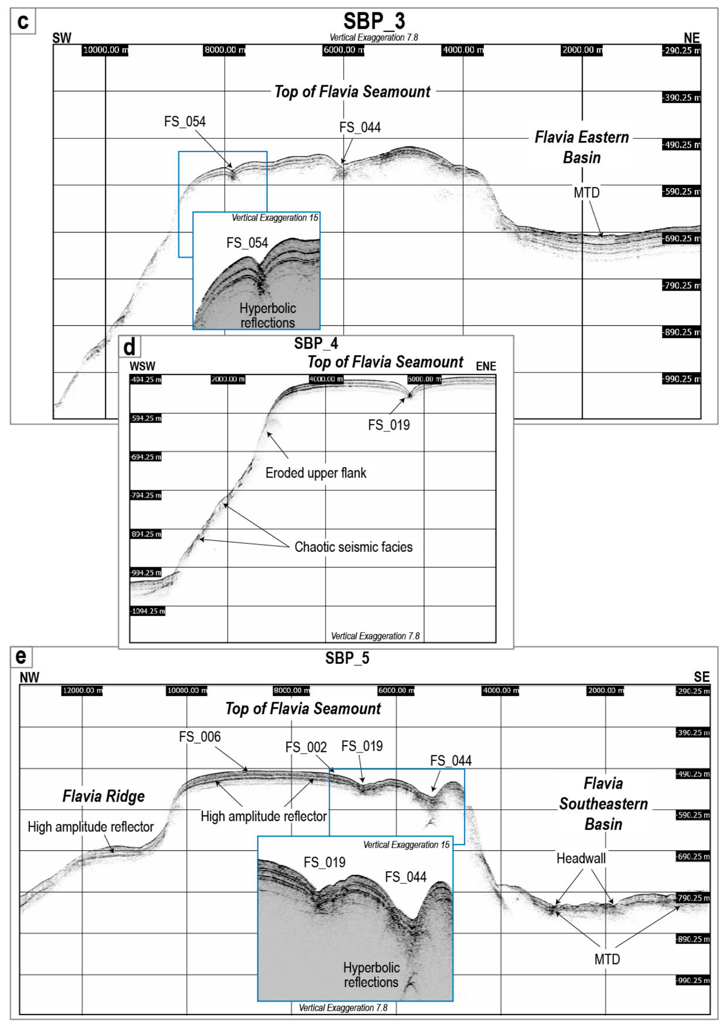
The SBP_3 profile, also SW–NE oriented, crosses the southern sector of the FS and the adjacent eastern basin (Figure 3c). Along this profile, the summit of the FS appears irregular due to the presence of several depressions, including pockmarks FS_054 and FS_044 (Supplementary Table S1), indicated by black arrows. In particular, the large depression FS_044 is associated with hyperbola-shaped seismic diffraction patterns within the acoustic basement (see the inset in Figure 3c). The sedimentary cover appears relatively undisturbed along the western flank, whereas it becomes more chaotic east of the FS. In the Flavia Eastern Basin, sedimentation is generally well preserved, with the exception of a shallow body at ~690 m depth, interpreted as an MTD (Figure 3c).

The WSW–ENE SBP_4 profile (Figure 3d) crosses the central part of the FS, emphasizing the steep western flank and the presence of chaotic deposits at its base. This profile also highlights pockmark FS_019 (Supplementary Table S1).

Finally, the SBP_5 profile (Figure 3e), oriented NW–SE, highlights in its northern sector a subtle positive seafloor relief corresponding to the Flavia Ridge (Figure 3a). This ridge is covered by at least ~45 m of layered sediments, locally interspersed with high-amplitude reflectors. The top of the FS is characterized by a ~35 m thick sedimentary cover, consistent with observations from the other profiles, and is locally affected by small hyperbolic reflections (diffractions). In its central segment, the profile crosses the FS from northwest to southeast, showing that the flat summit, where pockmarks FS_006 and FS_002 (Supplementary Table S1) are located, becomes progressively more irregular toward the southern sector, where the largest pockmarks (e.g., FS_019 and FS_044) occur. Notably, the internal seismic character changes beneath the pockmarks, particularly in correspondence with FS_044 (see inset in Figure 3e). In the southeastern portion of the profile, along the Flavia Southeastern Basin, several chaotic deposits are clearly visible. Here, the well-defined stratification observed at the summit of the FS is replaced by acoustically transparent units, indicative of coarse-grained material and associated with reduced seismic signal penetration. A prominent diffraction hyperbola is observed at approximately 65 m below the seafloor, which may indicate either the base of a depression or the presence of a localized gas accumulation.

Figure 3. (a) Shaded-relief map derived from the high-resolution multibeam bathymetry. The map was generated using Global Mapper software [33] in the UTM Zone 32N coordinate system (WGS84). Illumination parameters: sun elevation 70°, azimuth 330°, vertical exaggeration ×10. Brown contour lines represent isobaths (contour interval at 5 m). Magenta lines indicate the location of the time-to-depth converted SBP sections shown in this figure. The color palette used is “Roma” [34]. (b) SBP_2 profile, crossing the northern sector of the FS and the adjacent. (c) SBP_3 profile, crossing the southern sector of the FS and the adjacent eastern basin. (d) SBP_4 profile, crossing the central part of the FS. (e) SBP_5 profile, crossing the Flavia Ridge, the FS, and the southern sector of the study area.

Figure 3. (a) Shaded-relief map derived from the high-resolution multibeam bathymetry. The map was generated using Global Mapper software [33] in the UTM Zone 32N coordinate system (WGS84). Illumination parameters: sun elevation 70°, azimuth 330°, vertical exaggeration ×10. Brown contour lines represent isobaths (contour interval at 5 m). Magenta lines indicate the location of the time-to-depth converted SBP sections shown in this figure. The color palette used is “Roma” [34]. (b) SBP_2 profile, crossing the northern sector of the FS and the adjacent. (c) SBP_3 profile, crossing the southern sector of the FS and the adjacent eastern basin. (d) SBP_4 profile, crossing the central part of the FS. (e) SBP_5 profile, crossing the Flavia Ridge, the FS, and the southern sector of the study area.

Pockmark Statistical Analysis

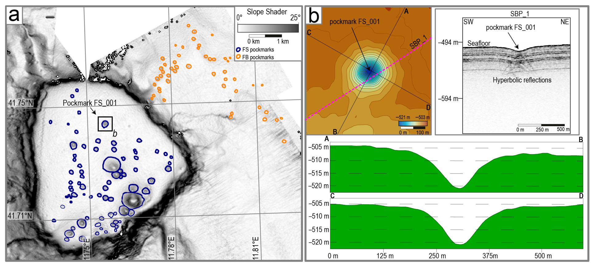
Based on the high-resolution bathymetric map (Figure 3a), a total of seventy-eight pockmarks were identified on the summit of the FS, whereas fifty-three occur within the basin east of the seamount (hereafter referred to as FB). Each pockmark was mapped (Figure 4a) and analyzed following a standardized methodology. This approach, conducted following [45,46], included assigning a unique identifier (ID) and recording the geographic coordinates of the deepest point, water depth, internal depth, perimeter, area, and circularity. The deepest point of each pockmark was identified through the generation of high-resolution bathymetric maps with a contour interval of 1 m and validated using two perpendicular bathymetric profiles crossing each depression, as illustrated in Figure 4b for the pockmark herein referred to as “FS_001”. Water depth was defined as the vertical distance between sea level and the deepest point of the pockmark. Internal depth was calculated as the vertical difference between the deepest point and the basal perimeter of the pockmark, corresponding to the blue and orange circles shown in Figure 4a. Figure 4b also presents a segment of the SBP_1 profile intersecting pockmark FS_001. Although the seismic profile does not cross the deepest portion of the depression, it still provides valuable information on its internal seismic character, highlighting features such as hyperbolic reflections.

Figure 4. Distribution of the bathymetric depressions and methodology adopted to quantify their morphometric parameters. (a) Slope-shaded map derived from the high-resolution multibeam bathymetry. The map was generated using Global Mapper software [33] in the UTM Zone 32N coordinate system (WGS84). Illumination parameters: sun elevation 70°, azimuth 330°, vertical exaggeration × 10. Blue circles delineate the perimeters of mapped pockmarks on the FS, whereas orange circles delineate those located in the basin east of FS. The black square highlights the area where the pockmark FS_001 has been identified; its characteristics are illustrated in panel (b). (b) Detailed view of pockmark FS_001. Upper left: high-resolution bathymetric map (contour interval at 1 m). Upper right: SBP_1 profile crossing the FS_001. Lower panels: bathymetric profiles crossing the FS_001 center along two perpendicular transects. The green fields indicate the seafloor morphology; the grey dashed lines indicate the depth below sea level.

Figure 4. Distribution of the bathymetric depressions and methodology adopted to quantify their morphometric parameters. (a) Slope-shaded map derived from the high-resolution multibeam bathymetry. The map was generated using Global Mapper software [33] in the UTM Zone 32N coordinate system (WGS84). Illumination parameters: sun elevation 70°, azimuth 330°, vertical exaggeration × 10. Blue circles delineate the perimeters of mapped pockmarks on the FS, whereas orange circles delineate those located in the basin east of FS. The black square highlights the area where the pockmark FS_001 has been identified; its characteristics are illustrated in panel (b). (b) Detailed view of pockmark FS_001. Upper left: high-resolution bathymetric map (contour interval at 1 m). Upper right: SBP_1 profile crossing the FS_001. Lower panels: bathymetric profiles crossing the FS_001 center along two perpendicular transects. The green fields indicate the seafloor morphology; the grey dashed lines indicate the depth below sea level.

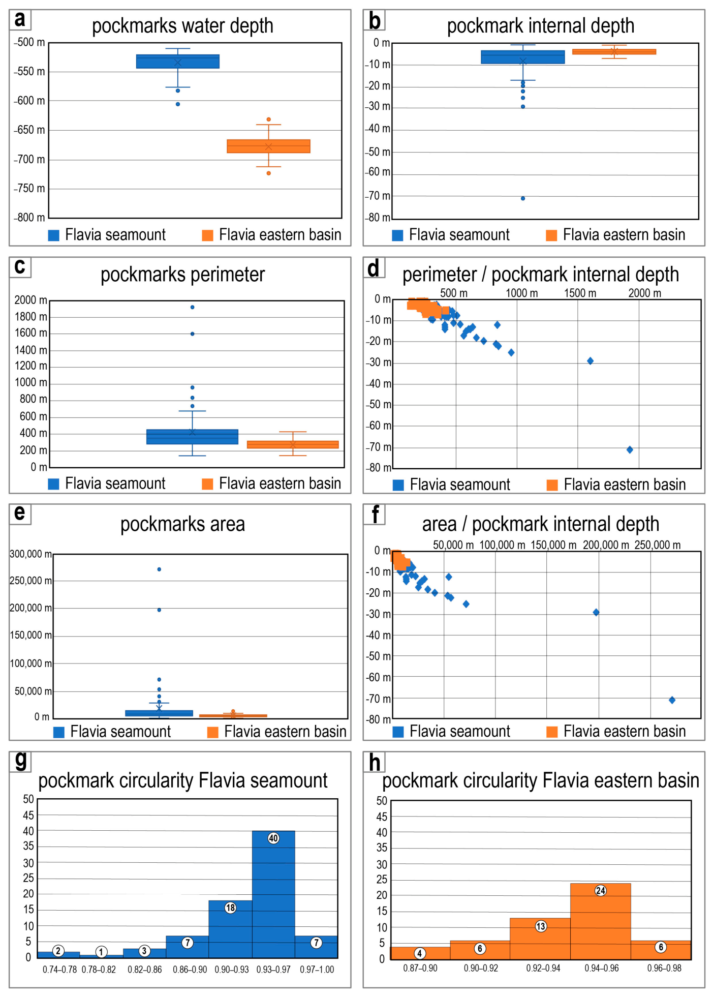
Figure 5a shows the distribution of pockmarks as a function of water depth, highlighting the presence of two distinct groups. Most pockmarks located on the summit of the FS (blue) fall within a depth range of 510–576 m b.s.l. (mean depth: −534 m), with the exception of three outliers at −578, −582, and −605 m (pockmarks FS_045, FS_054, and FS_044, respectively). In contrast, pockmarks within the FB (orange) are mainly distributed between 640 and 712 m b.s.l. (mean depth: −677 m), with two outliers at −631 and −723 m (pockmarks FB_001 and FB_023, respectively).

The internal depth of pockmarks (Figure 5b) is relatively homogeneous within the FB, ranging between 0.9 and 7 m (mean: 3.8 m). Conversely, pockmarks on the FS summit display a much wider variability, with internal depths ranging from 0.8 to 17 m (mean: 8.2 m), as well as several outliers between 18 and 29 m and a single extreme case reaching 71 m (pockmark FS_044).

Perimeter and area values, shown in Figure 5c,e, are relatively uniform for pockmarks within the FB (mean perimeter ~275 m; mean area ~5950 m²). In contrast, pockmarks on the FS summit exhibit a much broader variability: perimeter values range from 143 to 679 m, while areas range from ~16,000 to ~29,000 m². Several significant outliers are also present, including FS_044 (perimeter ~1922 m; area ~271,100 m²), FS_045 (perimeter ~961 m; area ~71,600 m²), and FS_050 (perimeter ~858 m; area ~56,900 m²).

This variability in the FS is further highlighted by the relationships between perimeter, water depth, and internal depth (Figure 5d,f), which confirm the greater homogeneity of morphometric parameters among pockmarks within the FB.

Additional statistical analysis of the size and geometry of the pockmarks was provided by calculating the circularity (C) for both pockmark populations using the following formula:

$$C={\displaystyle \frac{4\pi A}{P^2}}$$

where $\pi$ is the mathematical constant pi (~3.14), $A$ is the plan-view area of the pockmark and $P$ is the perimeter measured along its edge. Circularity values range from 0 (highly irregular, elongated, or elliptical pockmarks) to 1 (perfectly circular pockmarks). As shown in Figure 5g,h, both pockmark populations exhibit generally high circularity values, approaching those expected for a perfect circle, with the exception of a few outliers.

Figure 5. Statistical analysis of the main geomorphological parameters of pockmarks identified from the top of the FS and the FB: (a) water depth of pockmarks; (b) internal depth of pockmarks; (c) perimeter; (d) relationship between perimeter and internal depth; (e) area; (f) relationship between area and internal depth; (g) circularity distribution of pockmarks on the top of the FS; (h) circularity distribution of pockmarks in the FB.

Figure 5. Statistical analysis of the main geomorphological parameters of pockmarks identified from the top of the FS and the FB: (a) water depth of pockmarks; (b) internal depth of pockmarks; (c) perimeter; (d) relationship between perimeter and internal depth; (e) area; (f) relationship between area and internal depth; (g) circularity distribution of pockmarks on the top of the FS; (h) circularity distribution of pockmarks in the FB.

3.3. Sparker Seismic Profiles

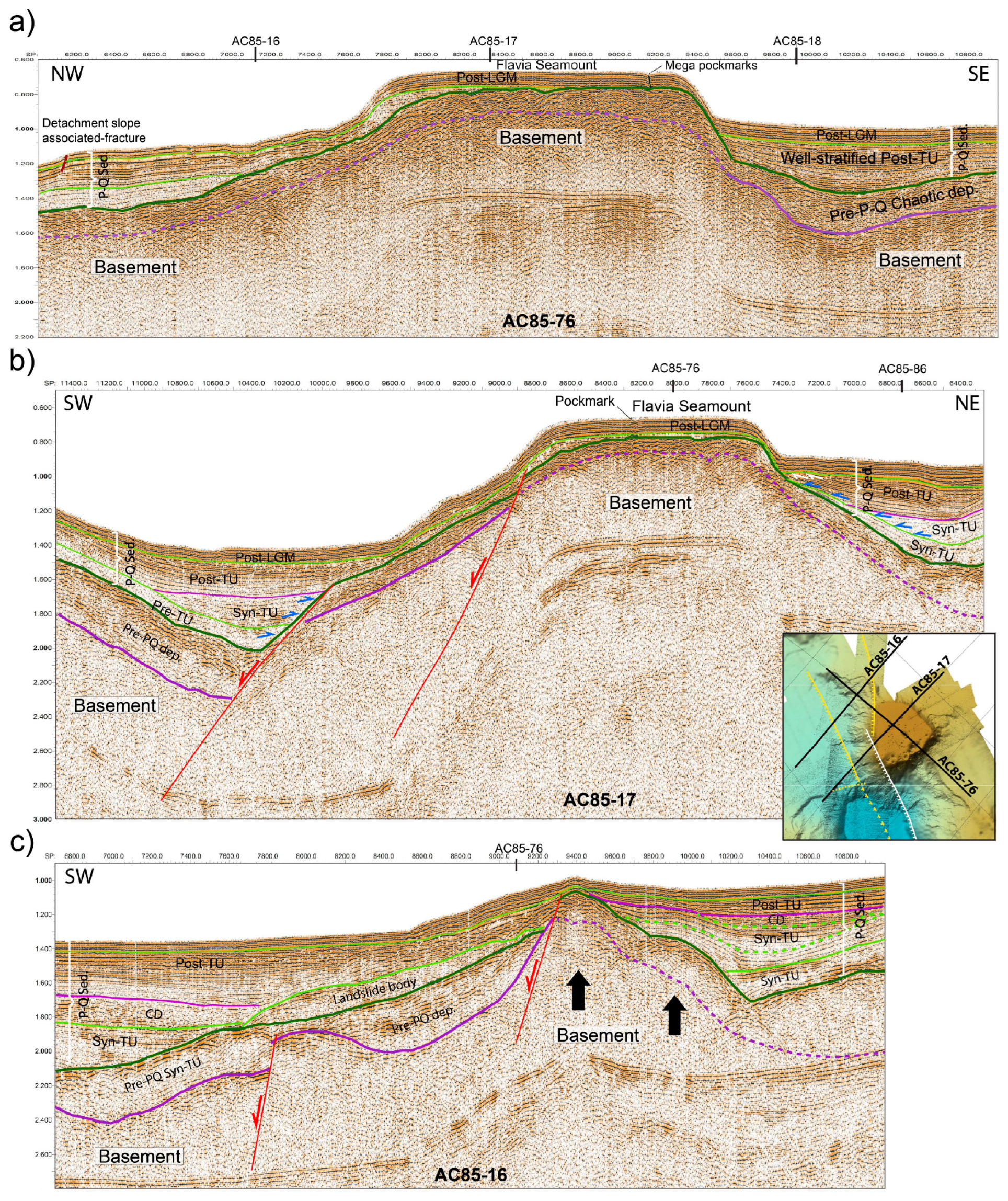
Unlike the SBP profiles shown in Figure 3, the three Sparker (30 kJ) seismic profiles interpreted in this study have sufficient resolution and penetration to identify the top of the acoustic basement, thereby providing key constraints for a more comprehensive tectonic interpretation of the main structural units. The faults identified in the interpreted seismic sections are displayed in yellow in the inset of Figure 6, whereas the fault shown in white is derived from regional tectonic maps available in the literature [18,30].

In the two parallel profiles with an approximately NE–SW orientation (AC85-17 and AC85-16; Figure 6), several sedimentary units are identified, some of which have been subdivided into pre-tectonic (pre-TU), syn-tectonic (syn-TU), and post-tectonic (post-TU) sub-units. This subdivision is primarily based on the geometry of the strata, as follows: (1) pre-TU units are sub-parallel to the underlying units on which they were deposited and display a relatively constant thickness across the basin; (2) syn-TU units exhibit a wedge-shaped geometry, thinning on one side and thickening on the opposite side, where they terminate in onlap onto the underlying units (blue arrows); (3) post-TU units show an almost constant thickness throughout the basin and appear largely undeformed, also terminating in onlap onto the underlying units (blue arrows).

The post-TU succession is overlain by an undeformed, well-stratified unit interpreted as young sediments draping the entire submerged surface, including the eroded top of the FS basement. Locally, the post-TU units display toplap terminations beneath this younger sedimentary cover (pink arrows), indicating localized erosion (Figure 6b).

A pre–Plio-Quaternary (pre-PQ) unit, identified in all analyzed profiles (Figure 6), is characterized by a well-defined upper reflector with high lateral continuity and strong amplitude. Internally, this unit exhibits poor reflectivity, and where present, reflectors are highly discontinuous.

Numerous large chaotic deposits and landslide bodies (CD), mapped in the AC85-16 seismic profile, are located at the transition between the syn-TU and post-TU units (Figure 6c). This profile intersects a margin that is currently extensively affected by slides and slumps (see map in Figure 6), clearly visible at the seafloor, which are actively eroding the northwestern flank of the FS.

Based on the geometry of the sedimentary units and underlying structures, east-dipping extensional faults, currently inactive, have been identified. These faults bound the northeastern sector of the FS and flank the Flavia Ridge, affecting the basement and the overlying sedimentary units up to the syn-TU level.

Figure 6. Sparker (30 Kj) AC85-76 (a), 17 (b) and 16 (c) sections, and their locations (see inset map). Red arrows indicate faults movement; blue arrows indicate the onlap of the seismic units. The yellow and white lines shown in the inset of Figure 6 represent faults according to literature [18,30]. TU: Tectonic Unit; P-Q Sed: Plio-Quaternary Sediments; CD: Chaotic Deposits.

Figure 6. Sparker (30 Kj) AC85-76 (a), 17 (b) and 16 (c) sections, and their locations (see inset map). Red arrows indicate faults movement; blue arrows indicate the onlap of the seismic units. The yellow and white lines shown in the inset of Figure 6 represent faults according to literature [18,30]. TU: Tectonic Unit; P-Q Sed: Plio-Quaternary Sediments; CD: Chaotic Deposits.

3.4. Magnetic Modelling

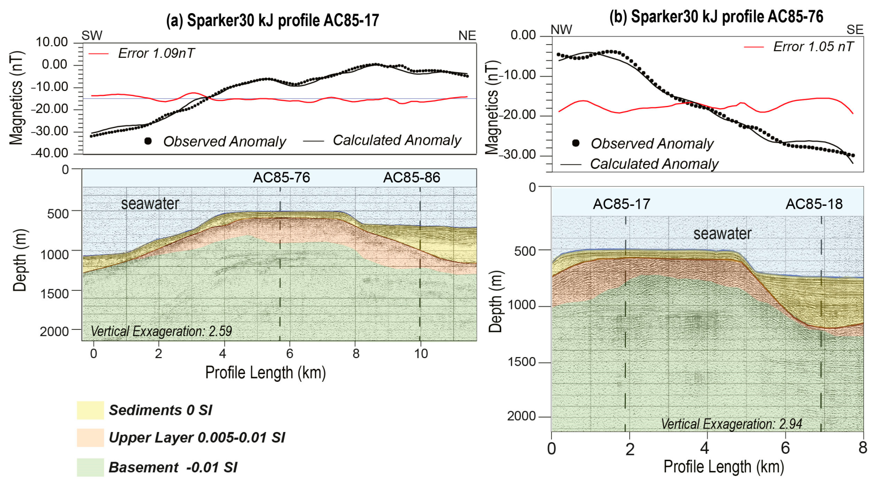
A forward-modelling approach was applied to the magnetic data to reconstruct the crustal structure beneath the FS region. In the present case, the interpretation benefited from a seismic stratigraphic framework derived from the depth conversion of part of Sparker 30 kJ profiles AC86-17 and AC85-76, which was used as the basis for the magnetic modelling. The two profiles, trending NE-SW and NW-SE, cross the area of interest and provide a simplified representation of its structural setting (Figure 6).

Figure 7. 2.5D forward magnetic modelling along selected segments of seismic Sparker 30 kJ profiles. (a) Model along profile AC85-17 (subset). (b) Model along profile AC85-76 (subset). The location of the profiles and the corresponding geophysical interpretation are shown in Figure 6. Upper panels: comparison between observed (dots) and calculated (solid line) magnetic anomalies; the average misfit (in nT) is also reported. Lower panels: interpreted distribution of magnetic susceptibility bodies derived from the depth-migrated seismic sections (shown as background), highlighting the geometry of the main lithological units. The grey lines indicate depth below sea level; the black dashed lines indicate the intersections with the Sparker 30 kJ lines AC85-17, 18, 76 and 86 [18,30].

Figure 7. 2.5D forward magnetic modelling along selected segments of seismic Sparker 30 kJ profiles. (a) Model along profile AC85-17 (subset). (b) Model along profile AC85-76 (subset). The location of the profiles and the corresponding geophysical interpretation are shown in Figure 6. Upper panels: comparison between observed (dots) and calculated (solid line) magnetic anomalies; the average misfit (in nT) is also reported. Lower panels: interpreted distribution of magnetic susceptibility bodies derived from the depth-migrated seismic sections (shown as background), highlighting the geometry of the main lithological units. The grey lines indicate depth below sea level; the black dashed lines indicate the intersections with the Sparker 30 kJ lines AC85-17, 18, 76 and 86 [18,30].

Given the limited length of the profiles and the resolution of the available data, the depth resolution of the modelling is constrained to a maximum of about 2 km. Based on the stratigraphic sequence observed in the seismic sections, both profiles reveal the presence of three main magnetic causative layers (Figure 7a,b): (i) a basement characterized by a slightly negative magnetic susceptibility value (−0.01 SI); (ii) an upper cover, mostly consisting of Quaternary marine sediments, showing no significant magnetic signature (0 SI); and (iii) an intermediate layer, referred to here as the “top layer”, between these two main crustal units, characterized by a slightly positive magnetic susceptibility of 0.005–0.01 SI and a variable thickness ranging from 200 to 500 m, with the maximum thickness observed at the western end of profile AC85-76 (Figure 7b).

This crustal level has an upper boundary consistent with the base of the Quaternary sediments, whereas its lower boundary is not resolved in the seismic data and is therefore inferred only from the magnetic susceptibility contrast using a best-fit approach between observed and computed magnetic anomaly profiles.

4. Discussion

4.1. New Insight into the Flavia Seamount

The FS is characterized by a flat, nearly circular summit and by an acoustic basement with a sub-horizontal top, overlain by a ~100 m-thick sedimentary unit composed of laterally continuous, sub-parallel seismic reflectors (Figure 2, Figure 3 and Figure 6). The FS displays a pronounced asymmetry (Figure 2 and Figure 3), with the southern flank reaching slopes greater than 30% (Figure 4). The western flank exhibits a concave-up upper sector and a convex lower sector, where chaotic seismic facies are observed (Figure 3b,d). The widespread occurrence of landslide scarps, chaotic deposits, and MTDs, particularly along the western flank and in the southeastern sector, suggests that repeated slope instability events have occurred. SBP and Sparker data (Figure 3 and Figure 6) show that these deposits are commonly located at the transition between syn-tectonic and post-tectonic units, indicating that slope failures were likely triggered during or shortly after tectonic activity. The presence of acoustically transparent units and disrupted stratification within the Flavia Eastern Basin (Figure 3e) further supports the interpretation of gravity-driven sediment redistribution [47,48]. Overall, these observations indicate that the FS has undergone significant post-depositional reworking, with mass-wasting processes having played a major role in shaping the present-day morphology [49,50].

The marked asymmetry of the FS also reflects structural control exerted by extensional tectonics. Sparker seismic profiles reveal east-dipping normal faults affecting both the basement and the overlying syn-tectonic units. These faults, although interpreted as no longer active because they do not offset the sedimentary succession overlying the acoustic basement, likely controlled the initial development of the seamount and adjacent basins, consistent with the extensional dynamics of back-arc settings [17,22].

The reduced-to-the-pole magnetic anomaly map of the FS area shows generally low anomaly values across the seamount (Figure 2b), approaching 0 nT, whereas more pronounced anomalies occur in the surrounding basins, particularly to the southwest and southeast (down to ~−40 nT). The highest positive magnetic anomalies are instead concentrated north of the FS, along the morphological feature here referred to as the Flavia Ridge. This spatial pattern suggests marked structural and compositional heterogeneity within the crust beneath the study area. The Flavia Ridge may represent either a localized magmatic intrusion having a felsic signature or a structural high associated with fault-controlled uplift, as also suggested by the geometry observed in Sparker profile AC85-16 (Figure 6c). This interpretation is consistent with previous studies highlighting localized magmatic contributions within extensional domains of the Tyrrhenian basin [13,16,18].

The FS therefore likely represents a tectonically controlled structural high whose flat summit reflects the combined effects of sedimentary draping, erosion, and extensional deformation, rather than the erosional truncation of a volcanic edifice during sub-aerial exposure. In the regional framework of the northern Tyrrhenian BAB, which is dominated by extensional deformation and characterized by rotational normal faults, tilted blocks, and half-graben and graben–horst systems [18,19,20,21,30,51,52,53], the FS can be compared to other structural highs in the northwestern Tyrrhenian basin, such as: (i) the Tiberino Seamount, located a few kilometers west of the FS and composed of continental crustal fragments and magmatic products [54]; (ii) the Albano Seamount [25]; and (iii) the Ponza–Palmarola structural high [55], whose seismic profile (TP6) closely resembles the Sparker profile AC85-17 interpreted in this study (Figure 6b).

4.2. Pockmarks Distribution and Fluid Circulation

Pockmarks in the FS area provide evidence for focused fluid migration within a morphologically and structurally heterogeneous setting. Their spatial distribution and morphometric variability indicate that fluid escape was not controlled by a single mechanism, but rather by the interplay among sedimentary architecture, mass-transport deposits, structural inheritance, and local slope instability. Two distinct pockmark populations have been identified in the study area: one located on the summit of the FS and the other within the adjacent FB. These two groups differ markedly in morphology, spatial organization, and associated seismic facies, suggesting the presence of two partially distinct fluid-migration domains.

Pockmarks within the FB are characterized by relatively homogeneous morphometric parameters, including limited variability in perimeter, area, and internal depth (Figure 5 and Supplementary Table S2). Their spatial distribution closely corresponds to sectors affected by chaotic seismic facies MTDs identified in the SBP profiles (Figure 3a). Furthermore, draped and weakly undulating sedimentary packages overlie these deposits, suggesting progressive sediment accumulation above an irregular and locally unstable substrate. The identification of a seismic chimney beneath a pockmark named “FB_014” provides direct evidence for vertically focused fluid migration through the sedimentary succession.

Taken together, these observations suggest that FB pockmarks are primarily related to fluid expulsion from overpressured sediments associated with MTDs and sediment loading processes. In such settings, MTDs may simultaneously act as low-permeability barriers and localized fluid reservoirs, promoting pore-pressure build-up and subsequent focused seepage through preferential pathways [47,48,56,57,58,59]. The relatively uniform geometry of FB pockmarks therefore suggests a comparatively stable, sediment-confined seepage system, in which fluid escape was primarily controlled by the physical properties and internal architecture of the basin infill rather than by strong structural heterogeneity.

In contrast, pockmarks located on the FS summit exhibit substantially greater variability in size, depth, and morphology, indicating a more complex developmental history than those identified within the FB. Several FS pockmarks display unusually large and irregular geometries, suggesting that their evolution was influenced not only by focused fluid escape but also by collapse-related processes, sediment remobilization, and repeated reactivation of pre-existing depressions [45,59,60,61].

The FS summit can therefore be interpreted as a structurally mediated fluid-migration domain, where inherited fault zones, uneven sediment loading, and local slope instability generated permeability contrasts that focused fluid ascent. In this setting, repeated seepage may have contributed to sediment weakening and progressive collapse, allowing some depressions to evolve beyond simple pockmark geometries. Pockmark “FS_044” represents the most prominent expression of this process: its anomalous size and depth, combined with disrupted seismic reflections and diffraction patterns observed in the SBP data, point to a composite seepage–collapse origin, possibly involving repeated reactivation of a pre-existing depression.

4.3. Challenges in the Classification of Submarine Reliefs in Complex Geodynamic Settings

According to [62], based on the International Hydrographic Organization (IHO) [63], a seamount is defined as “a discrete (or group of) large isolated elevation(s), greater than 1000 m in relief above the sea floor, characteristically of conical form”. Smaller isolated elevations rising less than 1000 m above the surrounding seafloor are commonly classified as knolls, whereas elongated features with a length-to-width ratio ≥ 2 are morphologically interpreted as ridges [64]. Finally, an isolated submarine elevation characterized by a relatively smooth flat summit is classically defined as a guyot [62,65].

This nomenclature is particularly effective in divergent oceanic settings and intraplate volcanic provinces, where submarine edifices commonly develop through relatively simple volcanic and subsidence histories. However, its application becomes less straightforward in tectonically complex environments such as continental margins, convergent systems, and back-arc basins, where seafloor morphology results from the interplay of tectonic deformation, sedimentation, magmatism, and gravitational processes.

The northern Tyrrhenian BAB represents a clear example of this complexity. Most of the bathymetric highs traditionally referred to as “seamounts” in the literature [24,25], including the Tiberino, Cialdi, and Etruschi edifices, do not exceed the 1000 m relief threshold required by the IHO definition and would therefore be more appropriately classified as knolls. Furthermore, several of these features exhibit elongated morphologies and would thus fall within the ridge category according to the morphometric framework proposed by [64]. This ambiguity is reflected in international marine nomenclature, where some structures are variably referred to as ridges rather than seamounts.

The classification of the FS is even more problematic. The FS does not exceed 1000 m of relief and therefore does not formally satisfy the IHO definition of a seamount. At the same time, its nearly circular morphology excludes classification as a ridge. From a purely geomorphological and stratigraphic perspective, the flat summit and sub-parallel sedimentary succession of the FH may superficially resemble a guyot [65]. Similar to classical guyots, seismic reflection data commonly reveal a planar surface overlying the acoustic basement and draped by sub-parallel sedimentary reflectors, locally interrupted by high-amplitude horizons interpreted as condensed intervals or non-depositional surfaces [66,67]. However, this interpretation becomes problematic when considering the geological and geodynamic context. Classical guyots are interpreted as volcanic edifices formed by intraplate magmatism, subsequently planed off by sub-aerial erosion near sea level and later submerged through thermal subsidence of the oceanic lithosphere [68,69]. Nevertheless, along convergent margins and BABs, including the Mariana–Izu–Bonin arc, the Parece Vela and Shikoku basins, and the Lau–Tonga system, flat-topped volcanic edifices are more commonly described as volcanic highs, remnant-arc edifices, or back-arc volcanic structures, reflecting the strong tectonic control exerted by these geodynamic settings [70,71,72,73].

The interpretation of the FS is further complicated by the lack of evidence for a volcanic basement. Instead, the FS developed within an extensional back-arc domain dominated by fault-controlled uplift and subsidence, syn-tectonic sedimentation, gravitational reworking, and localized magmatic intrusions.

These observations highlight the limitations of applying rigid morphometric classifications to submarine landforms developed in tectonically complex settings. In such environments, morphology alone may be insufficient to define the geological nature and evolutionary history of submarine edifices. For consistency with the existing regional literature and previous bathymetric atlases of the Tyrrhenian domain [24,25], the term “Flavia Seamount” is retained in this study, despite its imperfect correspondence with current geomorphological definitions.

5. Conclusions

This study provides the first integrated geophysical characterization of the FS, a previously poorly constrained geomorphological feature in the northeastern Tyrrhenian BAB. Although the FS superficially resembles a guyot, its flat summit and sedimentary cover are not supported by seismic and magnetic evidence for a simple volcanic origin. Instead, the FS is interpreted as a tectonically controlled structural high shaped by extensional deformation, sedimentary draping, and gravitational reworking, as indicated by inactive east-dipping faults, landslide scarps, chaotic deposits, and MTDs.

Morphometric and seismic analyses of pockmarks reveal two distinct fluid-migration domains: homogeneous basin pockmarks linked to MTD-related fluid escape, and more heterogeneous summit pockmarks reflecting the combined influence of seepage, structural inheritance, and gravitational processes.

Overall, this study highlights the importance of integrating multiple geophysical datasets to reconstruct the evolution of complex submarine systems and emphasizes the limitations of conventional geomorphological classifications when applied to tectonically active back-arc settings.