


Abstract
Ultra-High-Frequency (UHF) or Ultra-High-Resolution (UHR) seismic data can image in detail several meters below the seafloor, especially in shallow waters, where the assessment of the subsurface is critical for future nearshore construction. The method can detect the subsurface structure in detail in UHF seismic records, which are characterized by a high amount of diffracted energy. With the aim of enhancing the lateral continuity and resolution for the reflectors, we applied a multipath summation approach for the first time at such high frequencies. We employed strategies for separating the diffractions from the total signal in order to clearly take advantage of their AI-located apices for further velocity analysis. The derived Root Mean Square (RMS) velocity models did not prove to be sufficient for direct migration, something that the multipath summation using 2D stacking weights sufficiently solved. We combined the focused-energy seismic sections with the derived interval-velocity models and took into consideration the available borehole data to interpret the subsurface structure. We observed a sufficient enhancement of the P-wave refraction velocity models commonly derived in such investigations. This enhancement involved not only the resolution but also the additional indications of velocity reversals, which can be a severe drawback for the stability of offshore infrastructure due to the possibility of their hazardous origin, such as fractures, unstable bedrock, or voids.
1. Introduction
Seismic data formation is governed by linear wavefield superposition. The seismic energy from a source propagates through the subsurface along multiple trajectories generated by reflection, refraction, scattering, and diffraction. The recorded trace represents the summed response of these propagation paths in the 3D space. Imaging and velocity analysis, therefore, rely on reconstructing the travel paths of the seismic energy so that coherent events interfere constructively, while incoherent contributions are attenuated [1,2].
In seismic exploration, reflections cause laterally continuous reflectors that dominate seismic sections. However, small-scale heterogeneities such as fault tips, channel edges, fractures, and stratigraphic terminations scatter energy, creating wavefields carrying high-wavenumber structural information [3,4]. In unmigrated data, diffractions appear as hyperbolic events corresponding to the superposition of source–receiver wavepaths over a continuum of scattering angles [3,4,5]. Migration may be interpreted as a controlled inverse-summation operator that collapses these hyperbolae to their true spatial locations, which are their apices. The degree of diffraction focusing is highly sensitive to velocity accuracy and can therefore be exploited for model building.
A systematic framework for diffraction exploitation was introduced by Fomel et al. [3], who proposed post-stack velocity analysis based on diffraction separation and imaging. Further developments include multipath diffraction summation for shallow inhomogeneities [4], depth-domain diffraction migration [5], travel time-based diffraction enhancement [6], and sparsity-constrained least-squares path-summation imaging [7,8]. These approaches take advantage of the diffraction energy, treating it as a high-resolution carrier of structural information rather than as residual noise.
The principles of diffraction focusing were also extended to high-frequency electromagnetic imaging by Economou et al. [9], who introduced AI-assisted multipath summation strategies for GPR data. In these studies, machine learning identifies diffraction hyperbolae and constructs diffraction-consistent stacking weights, enabling the collapse of scattered energy and improving reflector continuity in heterogeneous media. Hamdan et al. [10] proposed adaptive stacking of constant-velocity migrated sections to enhance diffraction focusing without detailed velocity models. Together, these approaches demonstrate that coherent multipath summation—whether physics-driven or AI-assisted—can enhance both diffraction focusing and reflection continuity.
Multipath summation also governs reflector continuity enhancement. Normal moveout correction and stacking align coherent arrivals from laterally continuous reflectors, increasing signal-to-noise ratio through constructive interference [11]. Kirchhoff and wave-equation migration further improve continuity by repositioning dipping events and summing amplitudes along physically consistent travel paths [12,13,14,15]. The accuracy of these procedures depends directly on the sufficiency and the resolution of the assumed velocity model [16,17].
Ultra-high-frequency (UHF) seismic data acquired with offshore pinger systems introduce additional challenges. Operating in the kilohertz range, these systems produce wavelengths comparable to meter-scale sedimentary heterogeneities in shallow marine environments [18,19], resulting in scattering and recordings including diffractions masking the reflectors. While UHF acquisition provides enhanced vertical resolution, it also increases sensitivity to velocity errors, incoherent noise, and water-bottom multiples [18]. Under these conditions, incomplete migration creates residual diffraction tails and degraded reflector continuity.
Wave-equation-based imaging, including reverse time migration and one-way extrapolation methods, inherently accounts for complex multipath propagation and backscattered energy [13,14,16]. However, shallow offshore pinger surveys often rely on simplified or laterally smooth velocity models due to limited well control and inaccurate velocity models. In this setting, diffraction-focusing behavior provides a practical mechanism for evaluating velocity adequacy and assuring model refinement.
The objective of this study is to investigate the efficiency of multipath summation for diffraction focusing and reflector continuity enhancement in ultra-high-frequency offshore pinger data, as well as the usefulness of diffraction analysis for P-wave velocity model estimation. Even though Economou et al. [9,17] suggested that a diffraction velocity model on waveform data may not be sufficient for migration and interpretation, here we will demonstrate that this is not the case from UHF seismic data. Building on diffraction-guided velocity analysis [3,17], multipath diffraction summation techniques [4,7,9], and adaptive-AI-assisted stacking strategies [9,10], we assess how coherent summation of propagation paths can (i) improve lateral resolution and reflections continuity in shallow marine sediments, and (ii) provide a sensitive indicator of increased resolution seismic velocity model in UHF seismic surveys.
2. Materials and Methods
Sub-bottom profilers (SBPs) are high-resolution single-channel seismic systems using signals in the frequency range of 2–15 kHz. They can provide real-time high-resolution seismic reflection sections of the seafloor and the shallow subsurface. A typical application is the geotechnical assessment of the seafloor to support future offshore developments, such as marinas, wind farms, and other coastal infrastructure. There are multiple styles of SBP systems, each with advantages and disadvantages, defined by the way they generate, receive, and process the signal. The common types include [18]: (i) Pinger, Parametric (ii) Chirp (iii) Boomer or Sparker systems. Pinger, Parametric, and chirp type instruments are sometimes grouped together as ‘pinger’, which is a catch-all for high-frequency, high-resolution profilers targeting the sediments associated with the immediate seabed. They often utilize the same transducer to send and receive. Boomer and Sparker profilers are typically recognized as lower-frequency, deeper-penetrating systems that use separate sources and receivers. This paper discusses the use of a parametric profiler that emits high-frequency pulses at slightly different frequencies, which combine to form a focused low-frequency pulse capable of penetrating the sediments. The transducer acts as both the source and receiver. Pinger, parametric, and chirp systems have several advantages, such as ease of use and maintenance, portability, and the ability to support high ping rates. Pinger and parametric type instruments commonly utilize a narrow frequency band, resulting in a long signal with, in practice, several oscillations that reduce resolution. Chirp systems attempt to overcome this with a frequency sweep; however, as previously mentioned, each subsystem has its advantages and disadvantages, and the final instrument choice can come down to deployment method, required power, portability, and availability considerations, with the end product providing similar results in modern, commercially competitive systems. Moving forward, we group the pinger and parametric instruments under the common ‘pinger’ system, which is, at present, a more recognized SBP sub-system name. This paper discusses the style of a single transducer, fixed-frequency system. Resolution of a seismic section can be increased by deconvolution (temporal) and migration (lateral). If pinger’s dominant frequency provides sufficient temporal resolution and the depth of research is reached, then only the in-line lateral resolution could be increased if a sufficient scattered energy focusing scheme is introduced.
Migrations inherently lower the resolution, while multi-focusing techniques use stacking of migrated sections and increase this phenomenon, requiring spectral whitening techniques as a final step [10]. Multi-focusing techniques commonly apply a number of constant-velocity migrations to estimate a focusing assessment attribute, for example, kurtosis [3] or local slopes [17]. The scope of this estimation can be the generation of a migration velocity model [7], or only direct focusing without a velocity model using constant-velocity migrated sections weighted stacking (multi-path summation) [9,19]. Here, we will perform diffraction analysis to examine whether a diffraction velocity model can provide a sufficient way to enhance the interpretation of the depth sections of the UHF data based on borehole data, and to demonstrate that multi-path summation is the optimal additional use of this diffraction velocity model, rather than migration. The proposed methodology employs the following steps.
- (1)
- Data pre-processing of seismic section.
- (2)
- AI mapping of diffraction hyperbolas.
- (3)
- Estimation of the diffraction velocity and interval velocity models.
- (4)
- Stacking weights estimation.
- (5)
- Constant velocity time migrations and weighted stacking of time-migrated sections
These processing steps are described in more detail below. For the implementation we utilized Matlab R2022b in-house algorithms.
2.1. Pre-Processing of UHF Seismic Section
The common processing scheme for SBP data consists of some delay-time correction, band-pass filtering, time-varying gain, and envelope calculations. Further processing, like deconvolution or migration, may be used to enhance the section’s interpretability [18]. Here, we applied delay-time corrections, band-pass filtering using a trapezoidal filter with edges at 1000 Hz, 4000 Hz, 8000 Hz, and 12,000 Hz, and inverse-amplitude decay-time-varying gain, where necessary, for the final plots. Here, the signal involved is of a dominant frequency of 6400 Hz, and assuming that this frequency provides sufficient temporal resolution, we enriched the processing sequence by focusing the scattered energy, which enhances the lateral in-line resolution. Focusing on diffractions is commonly implemented by migration. Here, we propose the multipath summation method for this [4,17]. For either direct migration or the proposed methodology, a velocity model is required. For the estimation of a velocity model, we propose diffraction analysis [3,5].
Before going into a diffraction analysis sequence, the diffractions should be enhanced [3,7,19]. Enhancement is mainly referred to as isolating the diffraction energy, or separating it by the reflectors. There are different types of diffraction energy enhancement, such as the Plane-Wave-Destruction method [3,17], or reflection killers such as the damped rank-reduction method (DRR) [20]. We adopt the DRR method because, in addition to enhancing the diffraction energy, it also subtracts the reflections, thus providing the latter for further use.
2.2. Adaptive-AI Diffraction Analysis
Diffraction analysis involves straight-line fitting over the detected hyperbolas (x,t) points. This is implemented after adaptive diffraction mapping over the x-t plane with the use of a modification of the machine learning algorithm (ML) in [21], which involves connected clusters across neighboring traces and hyperbola fitting. The algorithm first selects regions of interest and reduces them by finding connected clusters on neighboring traces. The main steps of diffraction detection are:
- Image thresholding using an edge detector
- Raster images column segment and connection of elements
These imaging processing steps of the ML algorithm are applied to images after transforming the seismic section to a raster image.
We modified the C3 algorithm of Dou et al. [21] to automatically provide the estimated seismic RMS velocity for every diffraction and used the already trained model they provided. We involved the estimation of the EM diffraction velocity for each detected hyperbola within the detection algorithm, based on the diffraction’s kinematic characteristics.
2.3. P-Wave Velocity Models Estimation
The estimated velocity value corresponding to an apex of each one of the located diffractions is taken as the Root-Mean-Square (RMS) velocity value. Each velocity value was chosen to contribute to the initial RMS velocity model if it was within a specified range of velocity values guided by the minimum and maximum P-wave velocity values of a refraction survey. The P-wave velocity model from the refraction survey is an interval velocity model in depth. Transforming the interval velocity model in time leads to the estimation of the VRMS velocity model, based on each one of the interval velocity values Vi and the corresponding time Δti.
Minimum and maximum values of this velocity model specify the range of the diffraction velocities kept for the creation of the diffraction velocity model. The diffraction velocities are then interpolated to cover the whole section in time to create the VRMS diffraction model over each time value t, which in its turn is transformed to an interval velocity model Vint for each trace by
This model can be used for the enhancement of the interpretation of the seismic section, while the VRMS diffraction model is used for the estimation of stacking weights.
2.4. Stacking Weights Creation
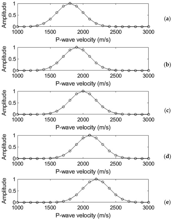
A velocity range with limits (i.e., 1000 m/s to 3000 m/s in the real data example case below) is created, which is further used for the estimation of the stacking weights. A second-level velocity range is created based on the minimum and maximum values of the RMS velocity model at the previous step. This range consists of values with a 100 m/s step (i.e., 1800 m/s, 1900 m/s, 2000 m/s, 2100 m/s, 2200 m/s in the real data example below). We create 2D stacking Gaussian weights for each of the second-level velocity ranges (i.e., 5 in our case), which are based on the weights depicted in Figure 1. For each 2D stacking weight section, each one of the velocity values within the VRMS diffraction model corresponds to a specific weight. For example, for the velocity value of 1800 m/s, the 2D weights section is created by assigning the weight values from Figure 1a for each one of the velocities in the VRMS section.
Figure 1.
One-dimensional weights on which the 2D weighting methodology is based. (a) The weights used for the 2D weights creation used for weighting the seismic section migrated by constant velocity of 1800 m/s, (b) 1900 m/s, (c) 2000 m/s, (d) 2100 m/s, and (e) 2200 m/s.
2.5. Multiple Time Migrations and Weighting Multipath Summation
The second-level velocity range referred to in the previous step is used for constant-velocity migrations of the initial data section. Note that, even though the velocity information is based on the diffractions-enhanced seismic section (with reflections suppressed), the migrations are applied to the initial section, which contains both the diffractions and the reflections. Hadamard multiplications of each constant velocity migration section with the corresponding 2D weights section, and the sum of all the products results in the final focused seismic section. Hadamard multiplication between two matrices corresponds to an element-by-element multiplication. This section does not correspond to a specific velocity value or model, but rather to a range of velocities. The diffractions are efficiently focused, avoiding artifacts from over- or under-migration in specific areas within the section, which would very possibly happen by using the migration velocity model and one-time migration. The procedure of weighted stacking is given by [8,9,10]
where B(x, t, u1, u2) is the multipath summation seismic section, A(x,t) is the initial seismic section, and Am(x,t,u) is the migrated seismic section using a constant velocity value u. G(x,t,u) is a 2D weighting function with its maximum equal to unity and is a Hadamard operator. The processing steps mentioned above are the basis for the creation of a focused seismic depth section and an interval-velocity depth model, which can be combined for the interpretation of the shallow offshore subsurface structure.
Concluding, the specific processing stages of the final step are epigrammatically
- Constant velocity migrations of the seismic section, using a specific velocity range (e.g., Figure 1, within the range of 1800 m/s to 2200 m/s, with a 100 m/s step, which is 5 migrations).
- Hadamard multiplication of each one of the constant velocity migrated sections with the corresponding weight.
- Summation of the products to produce the final multipath summation section.
3. Application to Offshore Data
3.1. Data Processing-Line 1
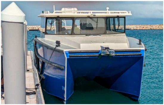
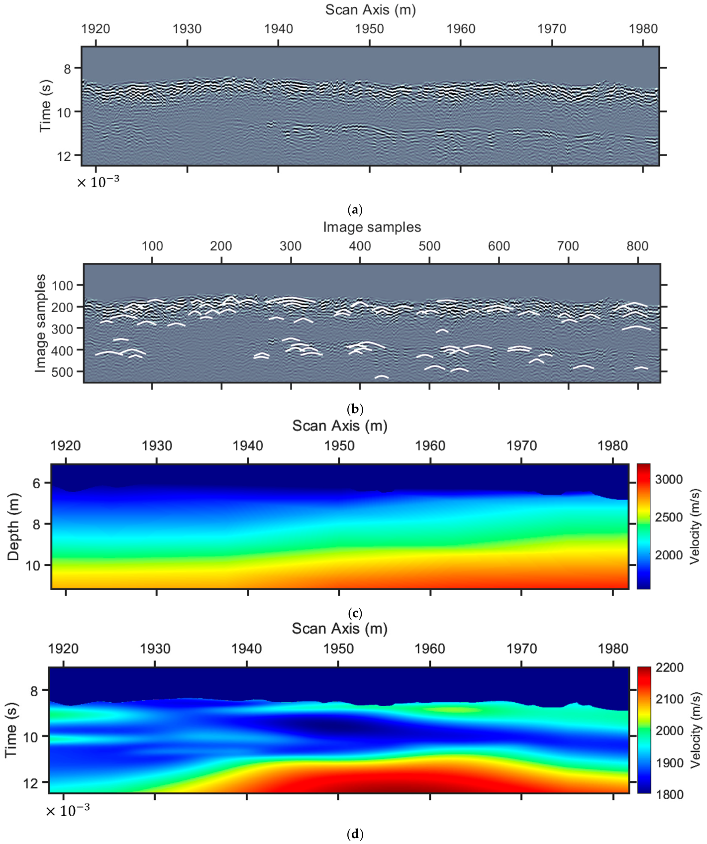
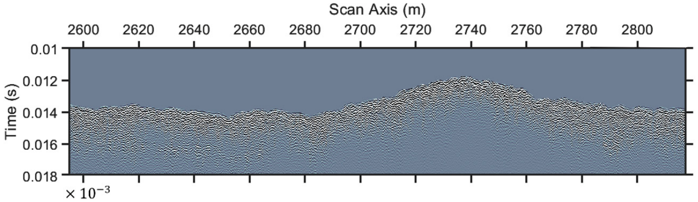
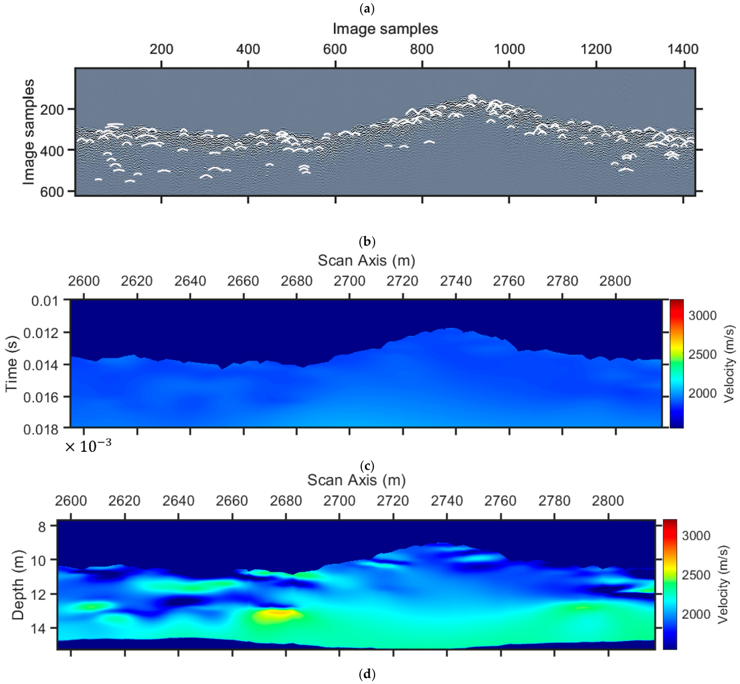
The proposed methodology was applied to UHF seismic data acquired at Western Australia and supplied by Surrich Hydrographics. The SBP equipment was a single-channel pinger system by Innomar. The data used here has a nominal peak frequency of 6 kHz. The transducer was mounted on a Pandu vessel (Figure 2), 0.45 m below the surface, and the nominal acquisition speed was 3 kn. A Geometrics GeoEel Continuous Marine Seismic Refraction (CMSR) system mounted on an “Interpid” vessel was also utilized, with a 24-channel digital streamer of 96 m total length and 2.34 m source offset, and a nominal speed of 1.5 kn. The scope was to assess the shallow subsurface for future offshore constructions. Although the target depth was deeper than in our study, we focus on the contribution of the Pinger system to the first 4 m below the seabed (Figure 3a). At first glance, there are two main reflectors, one at the shallowest part, which is due to the origin of the seafloor, and the second, which is the expected interface between shallow sediments and a calcareous formation. The transformation of the seismic section to a raster image creates the input to the C3 algorithm [9,21]. We use the algorithm of Dou et al. [21], modified by Economou et al. [9], who used a similar procedure for the diffractions’ location, but without using a diffraction killer filter; here we use the damped rank-reduction method from Chen et al. [20], to separate the diffractions section (Figure 3b) from the total seismic signal section (Figure 3a).
Figure 2.
Survey vessel “Pandu” operated by Surrich Hydrographics Pty Ltd.
Figure 3.
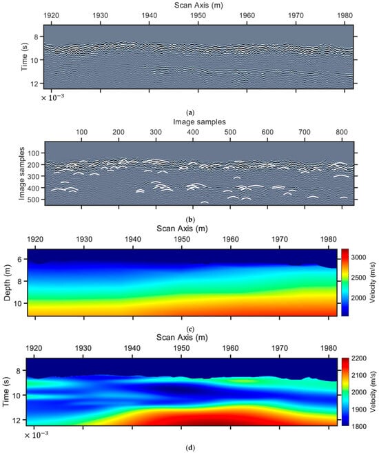
Diffraction analysis for the estimation of a migration velocity model for line 1. (a) Initial data after pre-processing, (b) adaptive-AI detected diffractions on (a) (white color) after diffractions enhancement (reflection killer filtering), (c) P-wave velocity profile from refraction survey, and (d) diffraction (RMS) velocity model from diffraction analysis. The vertical time axis is seconds × 10−3, as shown at the leftmost corner of the time sections.
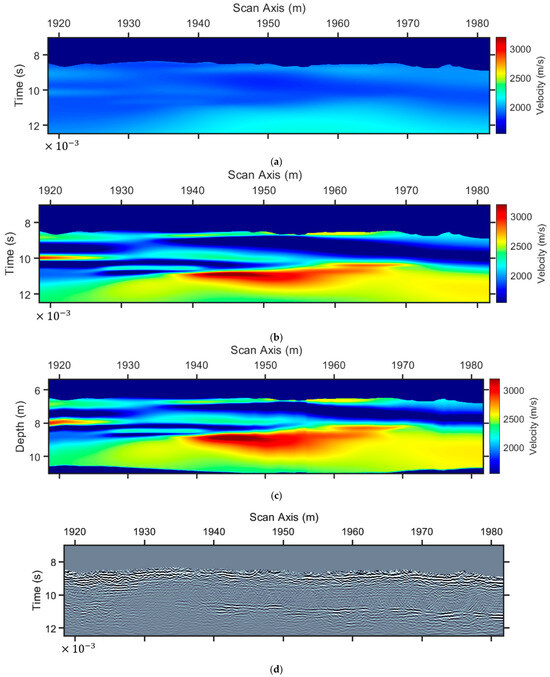
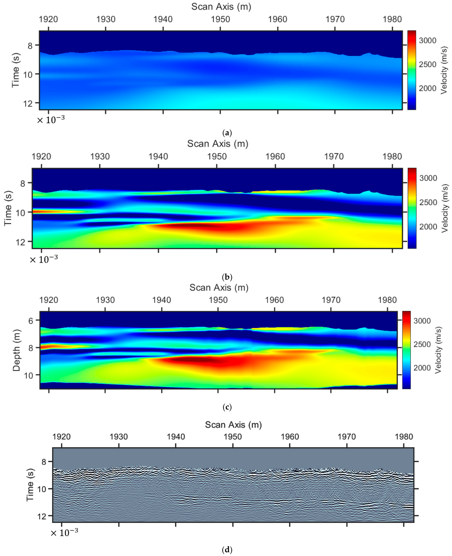
The CMSR method produced a refraction P-wave velocity model, as depicted in Figure 3c. With the scope estimate and the RMS velocity model from the diffractions shown in Figure 3b, we first created an RMS velocity model based on the refraction P-wave velocity model using Equation (1). We used the limits of this model as constraints for the interpolation of the diffraction (RMS) velocities. Our scope was to enhance the resolution of the P-wave velocity model in Figure 3b and to overcome the inherent drawback of the refraction method, which is the lack of sensitivity to velocity reversals. The lower velocity value was 1800 m/s, and the higher was 2200 m/s (Figure 3d), which, using the same color scale as that of Figure 3c, is depicted in Figure 4a. Using Equation (2), we generated the interval velocity model (Figure 4b) and the depth velocity model (Figure 4c). We further applied time migration to the seismic section depicted in Figure 3a, using the velocity model of Figure 4a. Several over-migrated areas, especially after 10 ms two-way travel time, indicate the need for a multipath summation approach [17].
Figure 4.
From the RMs velocity model to the interval velocity model and migration for line 1. (a) The RMS velocity model in Figure 3d with a different color scale, (b) interval velocity based on (a), (c) depth velocity model, and (d) migrated seismic section using (a). The vertical time axis is seconds × 10−3, as shown at the leftmost corner of the time sections.
The first step in weighted multipath summation is to migrate the seismic section with constant-velocity models. We utilized the range from 1800 m/s to 2200 m/s, which is the range of the velocity models (Figure 3c,d and Figure 4a). The step we used was 100 m/s, which yields the five velocity values mentioned in Figure 1. For greater heterogeneity, we could use a 50 m/s step, but one must always keep in mind that the larger the number of migrations, the higher the blurriness of the final stacked section [3,10,17].
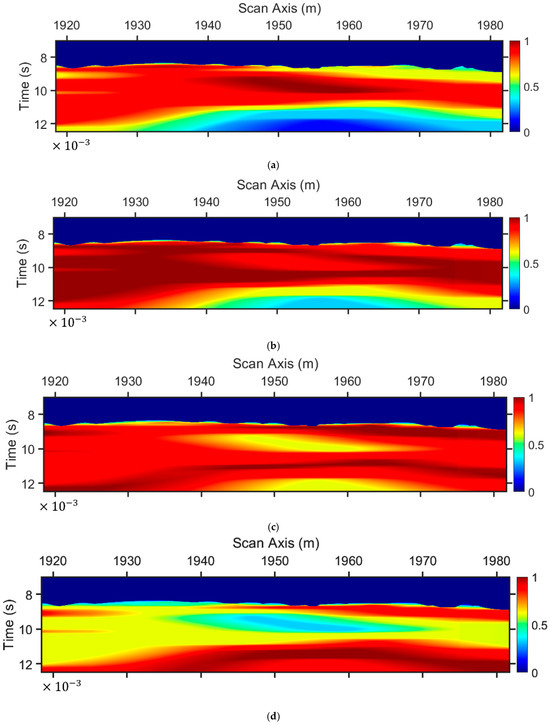
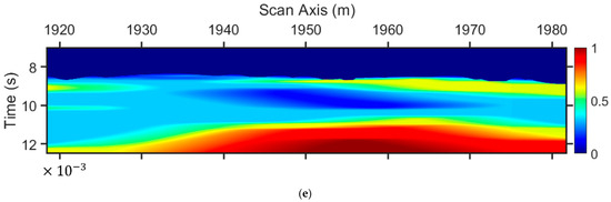
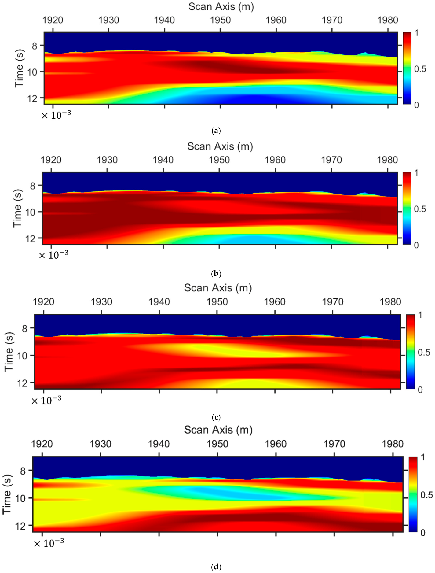
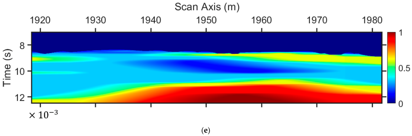
The next step is the 2D stacking weights estimation. For the constant velocity migrated section with 1800 m/s velocity, each value from the model depicted in Figure 3d obtained a weight value from the one-dimensional vector in Figure 1a for the creation of the 2D stacking weights in Figure 5a. For the weights in Figure 5b, the same model as in Figure 3d and the vector weights in Figure 1b were involved, and so on, until we have all the corresponding 2D weights. These were combined with the corresponding constant-velocity-migrated sections, and with the use of Equation (3), the multipath-summation section was generated (Figure 6a).
Figure 5.
Two-dimensional staking weights for line 1. (a) Stacking weights for the seismic section migrated with constant velocity 1800 m/s, (b) 1900 m/s, (c) 2000 m/s, (d) 2100 m/s, and (e) 2200 m/s. The vertical time axis is seconds × 10−3, as shown at the leftmost corner of the time sections.
Figure 6.
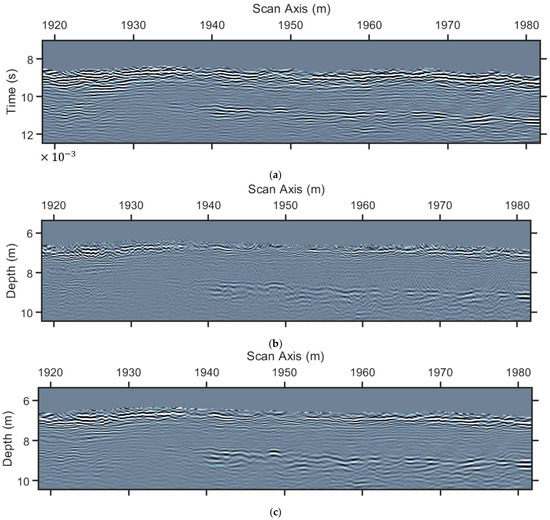
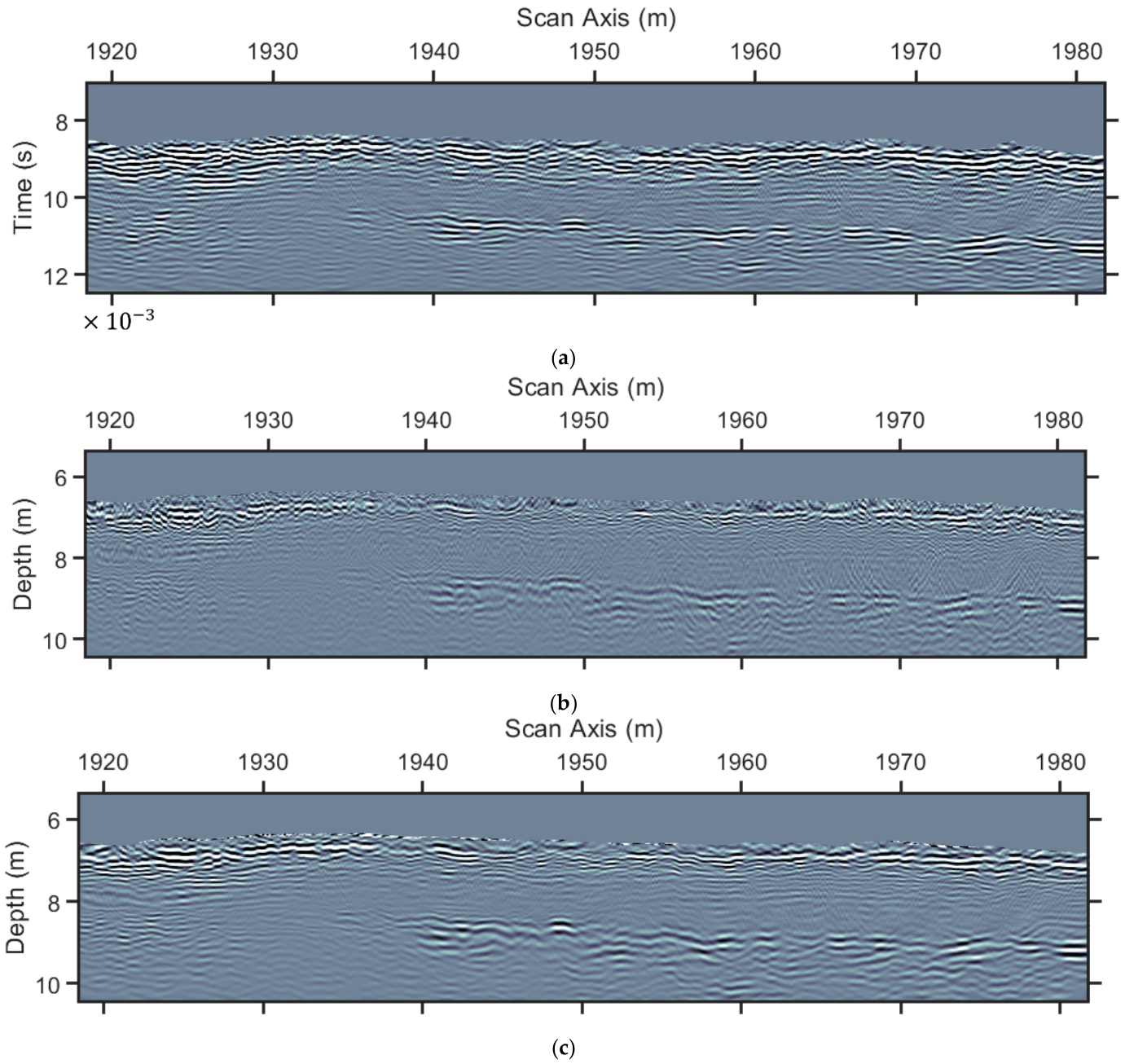
Multipath summation seismic section of line 1. (a) The seismic section depicted in 3a after multipath summation, (b) is 4d after time-to-depth conversion, and (c) is (a) after time-to-depth conversion. The velocity model for time-to-depth conversion is depicted in Figure 4a. The vertical time axis is seconds × 10−3, as shown at the leftmost corner of the time section.
Time-to-depth conversion was applied to the time -migrated seismic section depicted in Figure 4d (Figure 6b) and to the multipath summation section of Figure 6a (Figure 6c). For this transformation, we used the Dix conversion using (Equation (2)) and vertical-ray depth conversion [11,22].
This was implemented by first estimating the cumulative sums of the two-way travel times, which were transformed to depth using the interval velocity values. Then, for each time sample of the time-migrated seismic section, let a(t) denote the amplitude; it was interpolated to specific depth samples, with the minimum depth corresponding to the first time sample and the maximum depth to the maximum depth value from the previous step. The depth step was set to the distance corresponding to 1500 m/s, the velocity value of the water. Comparing the two sections in Figure 6b,c, one can observe a reduction in resolution with depth, which is due to the time-to-depth conversion. This was also mentioned by Biondi [22], who noted that time-to-depth conversion and depth migration squeeze or stretch the waveforms within the seismic section depending on the velocity values. Large velocity values stretch the waveforms as they are happening in the depth sections mentioned above. For this, and if the resolution is not considered sufficient for interpretation, one can additionally perform a zero-phase deconvolution [17].
The continuity of the reflectors was enhanced, as shown in Figure 6c, in comparison with the section in Figure 6b. The shallower reflector is clearly visible, and the reflector below 8 m depth is enhanced (Figure 6c). Also, minor reflectors in between 7 m and 8 m to the right part of the section are now clearer, and the reflector at the left part of the section at almost 8 m depth, which was not delineated clearly in Figure 6b, is now, after multipath summation, clear. This depth section can be used in combination with the estimated interval velocity model for further interpretation to delineate the subsurface structure of the area under investigation.
3.2. Data Processing-Line 2
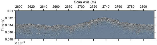
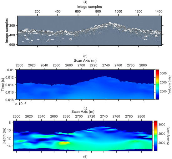
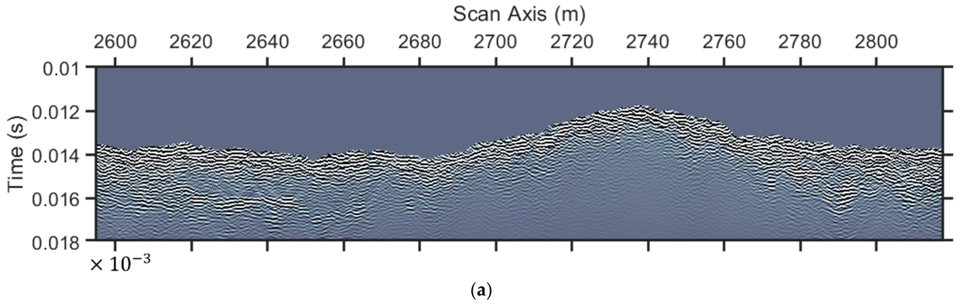
A similar data processing procedure was followed for line 2 (Figure 7). The initial data (Figure 7a) were under diffraction enhancement and adaptive AI-driven diffraction mapping (Figure 7b). The corresponding P-wave velocity range used as a constraint for the interpolation of the RMS velocity (Figure 7c) was estimated from a similar refraction velocity model, which ranged from 1800 to 2100 m/s. Following the transformation of this velocity section to Dix velocities, a depth conversion was conducted to the depth velocity model in Figure 7d.
Figure 7.
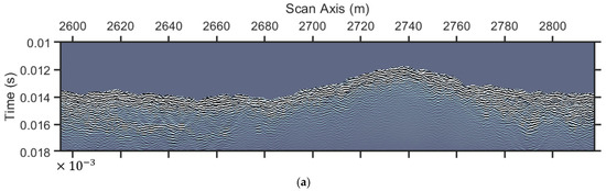
Diffraction analysis for the estimation of a migration velocity model for line 2. (a) Initial data after pre-processing, (b) adaptive-AI detected diffractions on (a) (white color) after diffractions enhancement, (c) diffraction (RMS) velocity model from diffraction analysis, and (d) depth velocity model. The vertical time axis is seconds × 10−3, as shown at the leftmost corner of the time sections.
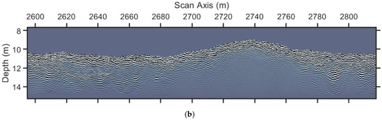
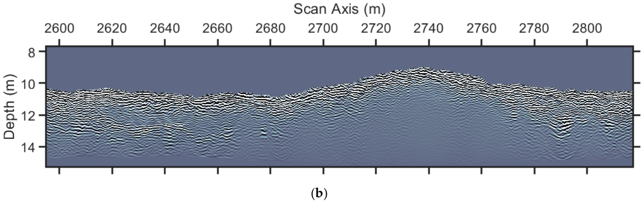
Constant velocity migrations using the aforementioned velocity range above and the estimation of the corresponding 2D weights in combination with Equation (3) led to the multipath summation depicted in Figure 8a, which, if compared to the section in Figure 7a, demonstrates the sufficient focusing of the diffracted energy and the enhancement of the continuity of the reflectors. A time-to-depth conversion results in the final depth section (Figure 8b).
Figure 8.
Seismic sections after multipath summation in line 2. (a) is Figure 7a after multipath summation, and (b) is (a) after time-to-depth conversion using the depth velocity mode depicted in Figure 7d. The vertical time axis is seconds × 10−3, as shown at the leftmost corner of the time section.
An example of the arbitrary squeeze or stretch of the waveforms can be seen at the reflector at around 13 m depth at the leftmost part, which is squeezed as it falls in a low velocity area (Figure 7d), in contrast to the reflector at the rightmost part at the same depth (Figure 8b). This final section, as the one from line 1, can be used for the delineation of the subsurface structure, with the additional borehole information existing for both lines.
3.3. Data Interpretation
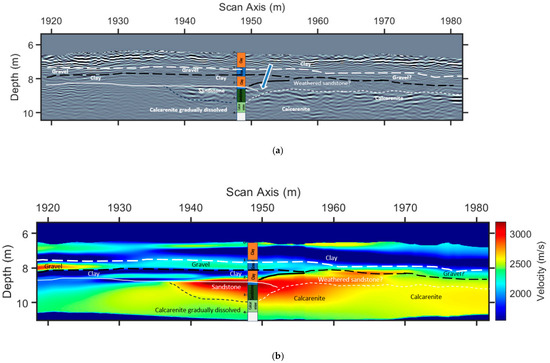
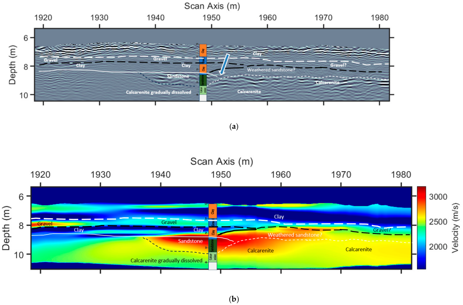
The main geological units existing in the area at the first meters are seabed sediments for the first 2–3 m in Line 1 and the first 8–9 m in Line 2, underlaid by the Tamala limestone unit. The former consists of clayey sands, sandy clays, and gravels, while the latter consists mainly of siliceous calcarenite and calcareous sandstone. Both geological units are imaged in seismic Section 1, while only the seabed sediments are mapped in Line 2. A combination of the estimated interval velocity model and the depth seismic section was used for the delineation of the subsurface structure (Figure 9). It is common practice to interpret the horizons (reflectors) in seismic depth sections using borehole information (Table 1 and Table 2) and local geology, and to extrapolate them based on their continuity (white lines in Figure 9 and Figure 10).
Figure 9.
Interpretation of the data from line 1. (a) The final depth section depicted in Figure 6c is interpreted, and (b) is the velocity model depicted in 4c interpreted. White lines are based on the seismic depth section in (a), and black lines are based on the velocity section in (b). Blue arrow in (a) indicates an unconformity or sandstone lens. The black arrow to the left of (b) indicates clays under gravel, and the black arrow to the right indicates dissolved formations below denser; both arrows indicate zones prone to instability. Upper reflections in (a) correspond to the heterogeneous interface between the seawater and the seabed.
Table 1.
Borehole samples description for line 1. The depths are referring to the sea bottom, which is zero depth for each case.
Table 2.
Borehole samples description for line 2. The depths are referring to the sea bottom, which is zero depth for each case.
Figure 10.
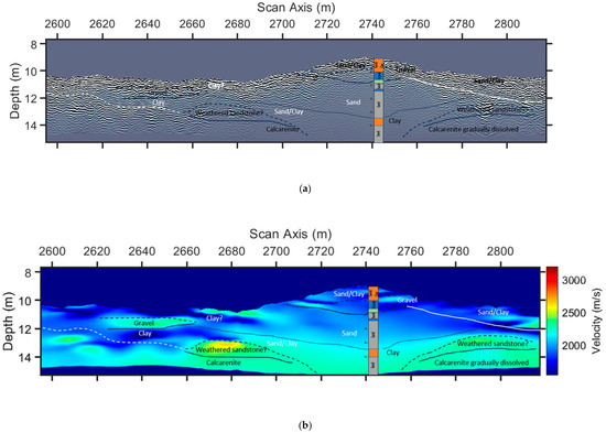
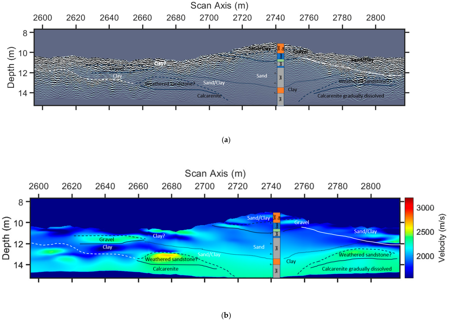
Interpretation of the data from line 2. (a) The final depth section depicted in Figure 8b is interpreted, and (b) is the velocity model depicted in Figure 7d interpreted. White lines are based on the seismic depth section in (a), and black lines are based on the velocity section in (b). Black arrows indicate clays below gravel, and the green arrow in the middle indicates a possible fault.
The available borehole information in-line (i.e., boreholes at positions less than 25 m from the study lines) with the sections is described below:
We went a step further by integrating the horizons and information from the velocity model to enhance interpretation details (Black lines in Figure 9 and Figure 10). Furthermore, the interpretation is constrained by the knowledge of the existing formations in the area based on other borehole information.
White lines delineate visible reflectors or seismic signal coherency or texture alterations, both the depth section and the velocity model (Figure 9a,b). Black lines are based on the interfaces denoted by interval velocity variations. A combination of both can be used to understand the formation’s extent, and it can also be seen that only one of them is not enough to follow the borehole information (Table 1). Borehole data almost at the middle of the Line 1 describe upper clays and gravel at the shallow part of the sea floor and down to almost 2.5 m below it, while lower calcareous sandstone and calcarenite follow (Figure 9a and Table 1). This continuous layered structure describes alterations of clays and gravel for the whole length of Line 1, while the lower clayey part seems to stop right of the borehole. Deeper, the sandstone formation (red color, Figure 9b) is not continuous, but rather has a lens form surrounding the borehole. This seems to be the densest formation in the area capable of hosting shallow offshore structures. Deeper, the calcarenite is not as dense as the sandstone, and borehole samples indicated core losses too, which denote a fragmented formation (Table 1). A comparison with Figure 3c, depicting the P-wave refraction velocity model, indicates the ability of the proposed methodology to image velocity reversals, which may be very important in the case of a project for the choice of the best places for foundations.
Overall, the main and most important issues prone to possible geohazards in Line 1 are the clayey layer under the gravel which may cause instability for the upper layers (Figure 9b, black arrow to the left side of the section), the gradual velocity values reduction in the calcarenite for the same reasons as mentioned before (Figure 9b, black arrow next to the borehole information) and the inconformity, or lens form of the sandstone, which even though is characterized as relatively dense, it “flows” over the more loose calcarenite (Figure 9a, blue arrow).
Line 2 followed the same procedure in the interpretation, with white lines based on the depth seismic section to indicate the visible alterations of the signal’s nature (Figure 10a). Black lines here indicate that the velocity model is much more useful in delineating the subsurface structure (Figure 10b). Additionally, the velocity model lacks accuracy at the middle part of Line 2, as can be seen in Figure 7a (horizontal sampling 800 to 1000 and vertical sampling below 300) and Figure 7c. This information gap is filled by the borehole information, indicating the need for all the available information to derive the subsurface structure nature (Table 2). This Line shows images mostly of shallow clays and gravel, with the deeper calcareous formations being lost at around 2740 m horizontal distance (Figure 10b), indicating also some parts where sandstone could provide places for future offshore structures foundations.
Concluding, the most important issues in Line 2 are summarized in the velocity reversal from the clayey formation over the gravel (Figure 10b, black arrow to the left part of the velocity section), which is a potential cause of instability of the overburden, the deep extend of the sandy/clayey formations near the borehole (Figure 10b, green arrow in the middle) indicating the loss of the calcareous formations possibly from a fault or fractured structure and the thick sandy/clayey formation below the gravelly shallow unit (Figure 10b, black arrow right from the borehole), which is also a unit prone to future slippery phenomena if the overburden is under stress. Finally, the calcarenite appears to be gradually fractured as in Line 1, which is a general issue needing further geotechnical studies.
The interpretation can be considered as a calibration for the seismic data and the corresponding velocity models, which can be very useful for the study of the velocities for the extended area. Based on the above conclusions and the literature [18,23,24], a table of representative velocities (Table 3) can be presented as follows:
Table 3.
Representative formations seismic P-velocities.
4. Discussion
With the scope to enhance the P-wave velocity model derived from the refraction method, in terms of both the resolution and the ability to describe velocity reversals, we demonstrated that a multipath summation method using 2D stacking weights on common-offset ultra-high-resolution seismic data can lead to a sufficient interpretation of the data. Borehole information evaluation and combination with the interfaces derived from both the reflections and the velocity alterations confirm the usefulness of the derived interval velocity models.
Our examples describe generally layered structures with slightly dipping at deeper parts with analogous velocity variations. Different formations, especially clayey and sandy formations above calcareous formations, cause textural differences with their surrounding environment within the seismic section image and reflections at times. The velocity models seem to give the most important information not seen at the seismic depth sections, especially for Line 2. The borehole information proves to be very important for the calibration, especially for verifying the very important for calibration, especially for verifying velocity reversals.
The density of diffractions located throughout the seismic section is an important factor for the sufficiency of the velocity model. Looking at Figure 3a and Figure 7b, one can observe areas with a few diffractions or no diffractions at all, and the velocity values derived by interpolation may be characterized as insufficient. For Line 1 (Figure 3b), the reflections are considered as sufficiently covered by diffractions, while the uncovered area lacks reflections. This can be taken as natural, not having a change in velocity, which is the case at the derived velocity model (Figure 3d). For Line 2, as it was already discussed, the lack of reflections and diffractions somewhere in the middle to the right deeper part is overcome with the borehole existence, which, if it did not exist, then the result could be insufficient.
An additional factor that should be taken into consideration is the 3D nature of the diffractions. Here, the 2D diffraction imaging and analysis are presented, and one of the problems could be the diffractions out-of-the-plane, i.e., diffractions outside the study line’s plane. These diffractions, if analyzed, correspond to higher-velocity information than the real velocity structure. This, together with the facts that diffractions are treated as having points as origin, and the possible high 3D heterogeneity of offshore environments, could bias the values in the final RMS velocity model. This enhances the value of the P-wave velocity model derived from the refraction experiment, which is used to set a floor and a ceiling on the estimated velocity values.
The 2D weights were not really commented within the manuscript, and one comment worth mentioning is that one may see a possibility for interpreting them, if one considers a formation having a mean velocity of 2200 m/s, for example, which could be fractured calcarenite. Then, following the high values (red color) at the specific 2D weights section, this specific formation is clearly delineated (Figure 5e). This raises a new issue and a future perspective for interpreting the weights, something that is currently out of the scope of the specific work.
Relatively high frequencies (acoustic/ultrasonic) generally produce slightly higher velocities than lower frequencies (1–100 Hz). Still, this dispersion is usually small, often 5% or less. The high porosity impact is more important, though. For example, as a cemented limestone, calcarenite has high porosity, often more than 30%, which keeps the velocity lower than sandstone or a non-porous limestone. Here, the sandstone is also calcite, which includes calcium carbonate, which significantly increases its density and thus its velocity. An additional effect on velocity is the compactness, which increases with depth, something very common for all kinds of seismic methods, which detect higher velocities with depth for the same formation.
Frequency-dependent attenuation is not considered here. Although the dominant frequency of the seismic signal decreases before reaching the seafloor, the investigated depths are limited to a few meters and therefore do not typically involve significant attenuation. Future efforts will focus on implementing a 3D approach, particularly for parallel survey lines, allowing diffractions to be analyzed in their inherently three-dimensional form, alongside the application of Full Waveform Inversion (FWI) to derive high-resolution velocity models. Initial implementations will use refraction-derived velocity models as background models, followed by further testing using the velocity models developed in this study. Still, one must have in mind that a smoothed velocity model permits FWI approaches to alter the velocities with iterations, while more detailed models may “trap” the velocity models and give solutions that are not sufficient.
5. Conclusions
We presented the application of diffractions focusing on UHF offshore seismic data, with the scope to improve reflection continuity and refine existing P-wave models obtained from refraction studies, which are typically employed in offshore geo-hazard assessments. For this, a multipath summation strategy efficiently focused the diffractions within seismic sections and aided in the derivation of interval velocity models describing the heterogeneity of the subsurface structure.
The kinematic characteristics of the diffractions, together with the existence of reflections and borehole data, overcome the lack of diffractions in specific areas, and sufficient interval-velocity models can be derived and used as calibration for future velocity interpretation.
We further showed that this method detects potentially hazardous velocity reversals, highlighting the inherent problem of the seismic refraction method, which can be a very important parameter, needing further research in these specific areas. This is particularly relevant in cases where the investigation aims to assess conditions for future offshore construction foundations.
Author Contributions
Conceptualization, N.E. and N.A.; methodology, N.E., N.A., M.Y.K., M.F., and J.A.; software, N.E. and N.A.; validation, N.E. and M.B.; formal analysis, N.A.; investigation, N.E. and J.A.; resources, N.E. and J.A.; writing—original draft preparation, N.E., N.A., J.A., M.Y.K., M.F., and M.B.; writing—review and editing, M.Y.K., M.F., and M.B. All authors have read and agreed to the published version of the manuscript.
Funding
This research received no external funding.
Data Availability Statement
Data is unavailable due to privacy restrictions.
Acknowledgments
We acknowledge Surrich Hydrographics Pty Ltd. for permitting us to publish the data.
Conflicts of Interest
Mr. Justin Anning is employed by Surrich Hydrographics Pty Ltd. The rest authors declare no conflicts of interest.
References
- Červený, V. Seismic Ray Theory; Cambridge University Press: Cambridge, UK, 2001. [Google Scholar]
- Bleistein, N.; Cohen, J.K.; Stockwell, J.W. Mathematics of Multidimensional Seismic Imaging, Migration, and Inversion; Springer Nature: Dordrecht, The Netherlands, 2001. [Google Scholar]
- Fomel, S.; Landa, E.; Taner, M.T. Poststack velocity analysis by separation and imaging of seismic diffractions. Geophysics 2007, 72, U89–U94. [Google Scholar] [CrossRef] [Scilit]
- Shin, J.; Ha, J.; Lim, K.; Lee, M. 3D diffraction imaging of channel and polka-dot anomalies in a shallow water area. Sci. Rep. 2026, 16, 19439. [Google Scholar] [CrossRef] [Scilit] [PubMed]
- Moser, T.J.; Howard, C.B. Diffraction imaging in depth. Geophys. Prospect. 2008, 56, 627–641. [Google Scholar] [CrossRef] [Scilit]
- Asgedom, E.G.; Gelius, L.J.; Tygel, M. 2D common-offset traveltime based diffraction enhancement and imaging. Geophys. Prospect. 2013, 61, 1178–1193. [Google Scholar]
- Merzlikin, D.; Fomel, S.; Sen, M.K. Least-squares path-summation diffraction imaging using sparsity constraints. Geophysics 2019, 84, S187–S200. [Google Scholar]
- Shtivelman, V.; Keydar, S. Imaging shallow subsurface inhomogeneities by 3D multipath diffraction summation. First Break 2005, 23, 39–42. [Google Scholar] [CrossRef] [Scilit]
- Economou, N.; Sobhi, N.; Al Abri, S.; Al Shaqsi, B.; Hamdan, H. AI Aided GPR Data Multipath Summation Using x-t Stacking Weights. In Proceedings of the 47th International Conference on Telecommunications and Signal Processing (TSP), Prague, Czech Republic, 10–12 July 2024; pp. 285–288. [Google Scholar] [CrossRef] [Scilit]
- Hamdan, H.; Economou, N.; Vafidis, A.; Bano, M.; Ortega-Ramirez, J. A new approach for adaptive GPR diffraction focusing. Remote Sens. 2022, 14, 2547. [Google Scholar] [CrossRef] [Scilit]
- Yilmaz, O. Seismic Data Analysis: Processing, Inversion, and Interpretation of Seismic Data; Society of Exploration on Geophysicists: Tulsa, OK, USA, 2001. [Google Scholar] [CrossRef] [Scilit]
- Schneider, W.A. Integral formulation for migration in two and three dimensions. Geophysics 1978, 43, 49–76. [Google Scholar] [CrossRef] [Scilit]
- Whitmore, N.D. Iterative depth migration by backward time propagation. Geophysics 1983, 48, 1514–1524. [Google Scholar]
- Baysal, E.; Kosloff, D.D.; Sherwood, J.W.C. Reverse time mi gration. Geophysics 1983, 48, 1514–1524. [Google Scholar]
- Gray, S.H.; Etgen, J.; Dellinger, J.; Whitmore, D. Seismic migration problems and solutions. Geophysics 2001, 66, 1622–1640. [Google Scholar] [CrossRef] [Scilit]
- Etgen, J.; Gray, S.; Zhang, Y. An overview of depth imaging in exploration geophysics. Geophysics 2009, 74, WCA5–WCA17. [Google Scholar] [CrossRef] [Scilit]
- Economou, N.; Vafidis, A.; Bano, M.; Hamdan, H.; Ortega-Ramirez, J. Ground-penetrating radar data diffraction focusing without a velocity model. Geophysics 2020, 85, H13–H24. [Google Scholar] [CrossRef] [Scilit]
- Dondurur, D. Acquisition and Processing of Marine Seismic Data; Elsevier: Amsterdam, The Netherlands, 2018. [Google Scholar] [CrossRef] [Scilit]
- Landa, E.; Keydar, S. Seismic monitoring of diffraction images for detection of local heterogeneities. Geophysics 1998, 63, 1093–1100. [Google Scholar] [CrossRef] [Scilit]
- Chen, Y.; Huang, W.; Yang, L.; Oboue, Y.A.S.I.; Saad, O.M.; Chen, Y.F. DRR: An open-source multi-platform package for the damped rank-reduction method and its applications in seismology. Comput. Geosci. 2023, 180, 10. [Google Scholar]
- Dou, Q.; Wei, L.; Magee, D.; Cohn, A. Real-Time Hyperbola Recognition and Fitting in GPR Data. IEEE Trans. Geosci. Remote Sens. 2017, 55, 51–62. [Google Scholar]
- Biondi, B. 3D Seismic Imaging; Investigations in Geophysics Series NO.14; Society of Exploration on Geophysicists: Tulsa, OK, USA, 2006. [Google Scholar]
- Novak, A.; Šmuc, A.; Poglajen, S.; Celarc, B.; Vrabec, M. Sound Velocity in a Thin Shallowly Submerged Terrestrial-Marine Quaternary Succession (Northern Adriatic Sea). Water 2020, 12, 560. [Google Scholar] [CrossRef] [Scilit]
- Holdgate, G.; Wallace, M.; Daniels, J.; Gallagher, S.; Keene, J.; Smith, A. Controls on Seaspray Group sonic velocities in the Gippsland Basin-A multidisciplinary approach to the canyon seismic velocity problem. APPEA J. 2000, 40, 295–312. [Google Scholar]

Disclaimer/Publisher’s Note: The statements, opinions and data contained in all publications are solely those of the individual author(s) and contributor(s) and not of MDPI and/or the editor(s). MDPI and/or the editor(s) disclaim responsibility for any injury to people or property resulting from any ideas, methods, instructions or products referred to in the content. |
© 2026 by the authors. Licensee MDPI, Basel, Switzerland. This article is an open access article distributed under the terms and conditions of the Creative Commons Attribution (CC BY) license.