Landslide Susceptibility on Mars: Application of Frequency Ratio Method

Abstract

Landslides are recognised as one of the most widespread mass-wasting processes that modify the surface of Mars. Understanding the distribution of these processes is essential for identifying areas where slope failure conditions may occur and the factors that most strongly influence their occurrence. This study utilises a Frequency Ratio (FR) landslide susceptibility method to a landslide inventory in Valles Marineris, considering three landslide types. The analysis involves conditioning factors derived from topographic and structural data. The results underline the influential role of morphometric parameters in controlling landslide occurrence, with steep slope classes and high local relief values showing the strongest positive correlations with landslide distribution. The predictive performance of the susceptibility models is supported by Area Under the Curve (AUC) values of 0.82 for Slumps, 0.78 for Rock Avalanches, and 0.75 for Debris Flows, indicating good model reliability. Proximity to tectonic structures appears to contribute to landslide occurrence, suggesting that structurally weakened rock masses or past seismic activity may influence slope instability in the region. Overall, the results display the potential of statistical landslide susceptibility approaches for analysing slope instability processes in planetary environments and provide a new toolkit for future investigations on Mars.

1. Introduction

The study of landslides has long been a central topic in geomorphological research, providing key insights into the surface dynamics of Earth and, more recently, of other planetary bodies. These gravity-driven processes offer valuable information about the geological, tectonic, environmental, and even internal evolution of the surfaces on which they occur. Although landslide investigations have traditionally focused on terrestrial environments [1,2], the growing availability of high-resolution data from orbital missions and planetary rovers has enabled the extension of such studies to airless bodies or planets characterised by extreme environmental conditions, including low gravity, the absence or rarity of an atmosphere, large temperature fluctuations, and the lack of liquid water. Notable examples include the Moon [3,4,5], Mars [6,7], Mercury [8], and several icy satellites in the Solar System [9,10]. Comparative analyses of landslides across these diverse planetary settings are therefore important not only for understanding local geological processes, but also for testing and validating theoretical models of slope instability under extreme physical conditions.

In this context, Mars stands out among planetary bodies for its morphological diversity and strong similarities to terrestrial landscapes, making it a natural laboratory for landslide studies. Large-scale landslide deposits have been documented since the Viking missions [11] and have since been examined in greater detail using high-resolution datasets from the Mars Orbiter Laser Altimeter (MOLA) [12], the High Resolution Imaging Science Experiment (HiRISE) [13], and the Context Camera (CTX) [14]. Early work by Lucchitta [15] emphasised the potential role of ground ice and wet debris flows in triggering slope failures. A subsequent study by Lucas & Mangeney [16] explored the influence of topography and slope mechanics on landslide mobility, introducing geomorphometric parameters specifically adapted to Martian environments. More recently, three-dimensional numerical modelling by Barzegar et al. [17] demonstrated the effectiveness of combining the Finite Element Method (FEM) with the Strength Reduction Method (SRM) to evaluate slope stability under Martian conditions. Schultz et al. [18] investigated the contribution of tectonic stresses to slope instability, while Discenza et al. [19] reported new evidence of mass wasting in Sisyphi Cavi, where internal material weakening and ice sublimation are proposed as key preparatory mechanisms.

Focusing on the specific study area analysed in this research, Valles Marineris represents one of the most extensively studied regions on Mars with respect to large-scale landslides, owing to its extreme relief, steep canyon walls, and widespread evidence of mass wasting. Early pioneering works by Lucchitta [20] documented numerous large landslide deposits within the canyon system and proposed that ground ice, transient liquid water, and debris flow processes may have played a significant role in slope failure initiation. Subsequent investigations refined the geomorphological classification of landslide types in Valles Marineris, identifying rock avalanches, rotational slides, and complex mass movement deposits (e.g., [21,22]). Using high-resolution orbital imagery and topographic datasets, researchers have analysed landslide runout, deposit morphology, and mobility, revealing unusually long travel distances that suggest low basal friction and potential lubrication mechanisms [23]. Later studies incorporated numerical modelling approaches to explore the mechanical behaviour and stability of canyon slopes, highlighting the influence of lithological layering, structural discontinuities, and seismic or tectonic forcing as potential destabilising factors [24]. More recent work has emphasised the role of volatile-rich materials, ice sublimation, and long-term internal weakening in preconditioning slopes to failure, reinforcing the interpretation of Valles Marineris as a key natural laboratory for understanding mass wasting under Martian environmental conditions [19].

Several regional and global investigations have examined the large-scale distribution of mass movements in Valles Marineris, providing a framework comparable to terrestrial landslide susceptibility analysis. Global inventories of Martian landslides reveal that Valles Marineris hosts one of the highest concentrations of slope failures on the planet, reflecting the combined influence of extreme relief, lithological heterogeneity, and tectonic weakening [25,26]. Spatial statistical analyses indicate that landslide occurrence is strongly correlated with morphometric parameters such as slope angle, local relief, elevation gradients, and curvature, supporting the interpretation that predisposing factors operate at regional rather than purely local scales [27]. Structural and tectonic studies further suggest that fracture networks, fault zones, and stress field orientations exert a first-order control on the spatial clustering of slope instabilities within the canyon system [28]. In addition, regional-scale geomorphological mapping of Martian canyons has highlighted systematic associations between mass-wasting deposits, layered bedrock units, and long-term erosional processes, reinforcing the view that landslide susceptibility in Valles Marineris is governed by persistent geological and mechanical controls rather than transient climatic forcing [29,30].

Within this framework, the main contribution of the present study lies in the application of a predictive statistical approach, widely used in terrestrial landslide susceptibility assessments, to the Valles Marineris region on Mars. While previous investigations have primarily focused on site-specific geomorphological analyses, kinematic reconstructions, or deterministic numerical modelling of slope failures, regional-scale approaches capable of spatially identifying areas potentially prone to landsliding remain limited to the work of Roback & Ehlmann [27].

In particular, the present work explores the spatial distribution of morphometric factors that may predispose canyon slopes to failure, with the aim of identifying sectors where the topographical and mechanical conditions could favour landslides potentially triggered by seismic shaking. The hypothesis that Martian landslides may be initiated by seismic activity related to tectonic stresses or impact-induced ground motion has been proposed in several studies, highlighting the importance of evaluating slope stability within a broader regional susceptibility framework (e.g., [31,32]).

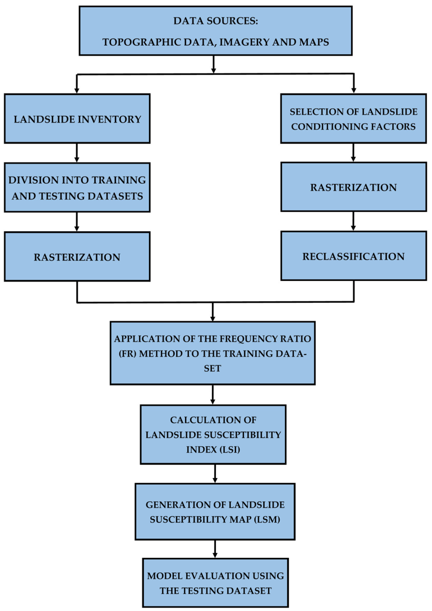
On Earth, landslide susceptibility mapping has become a consolidated tool in geomorphology and hazard assessment, relying on the statistical correlation between mapped landslide occurrences and a set of conditioning factors. Among the various approaches developed over the past decades, the Frequency Ratio (FR) method, summarised in Figure 1, has been extensively validated due to its conceptual simplicity, robustness, and effectiveness in identifying relationships between landslide distribution and environmental variables (e.g., [33,34]).

Transferring this methodology to Mars represents a significant methodological step. Unlike terrestrial contexts, where susceptibility modelling is often calibrated using field-based inventories, Martian applications must rely exclusively on remotely sensed topography and imagery. In this study, morphometric parameters derived from orbital Digital Elevation Models (DEMs) are statistically combined with geo-structural information related to extensional fault systems, which are here considered as proxies for tectonically induced seismic triggering.

More than treating landslides as a single homogeneous class, the inventory and modelling were subdivided into three major kinematic categories—Rock Avalanches, Slumps, and Debris Flows—each characterised by distinct mechanical behaviour, mobility patterns, and geomorphological signatures. On Earth, it is well established that different landslide types respond differently to conditioning factors [35,36]. Applying this conceptual framework to Mars allows the identification of differential controls on slope instability, providing insights into whether large rock avalanches are predominantly structurally controlled.

Despite decades of investigation, the precise interplay between mechanical, climatic, and cryogenic processes driving landslide activity in Valles Marineris remains an open research question. The present study does not aim to fully resolve this complex problem, but rather to provide a complementary methodological framework for investigating the spatial distribution of landslides under Martian environmental conditions. By integrating a comprehensive landslide inventory, morphometric predictors, structural datasets, and an independent validation procedure, this work transfers a susceptibility-mapping approach widely used in terrestrial contexts to the Valles Marineris region. In doing so, it moves beyond purely descriptive geomorphology and deterministic slope modelling by introducing a probabilistic and spatially explicit framework for assessing type-specific landslide susceptibility on Mars. Considering that mechanisms driving gravitational movements are fundamental, but they go beyond the scope of a landslide susceptibility study, this approach expands the methodological toolkit of planetary geomorphology and establishes a conceptual bridge between terrestrial hazard-oriented methods and extraterrestrial landscape analysis. It provides a basis for future studies that may incorporate more detailed lithological, geotechnical, climatic, and cryogenic information.

2. Study Area

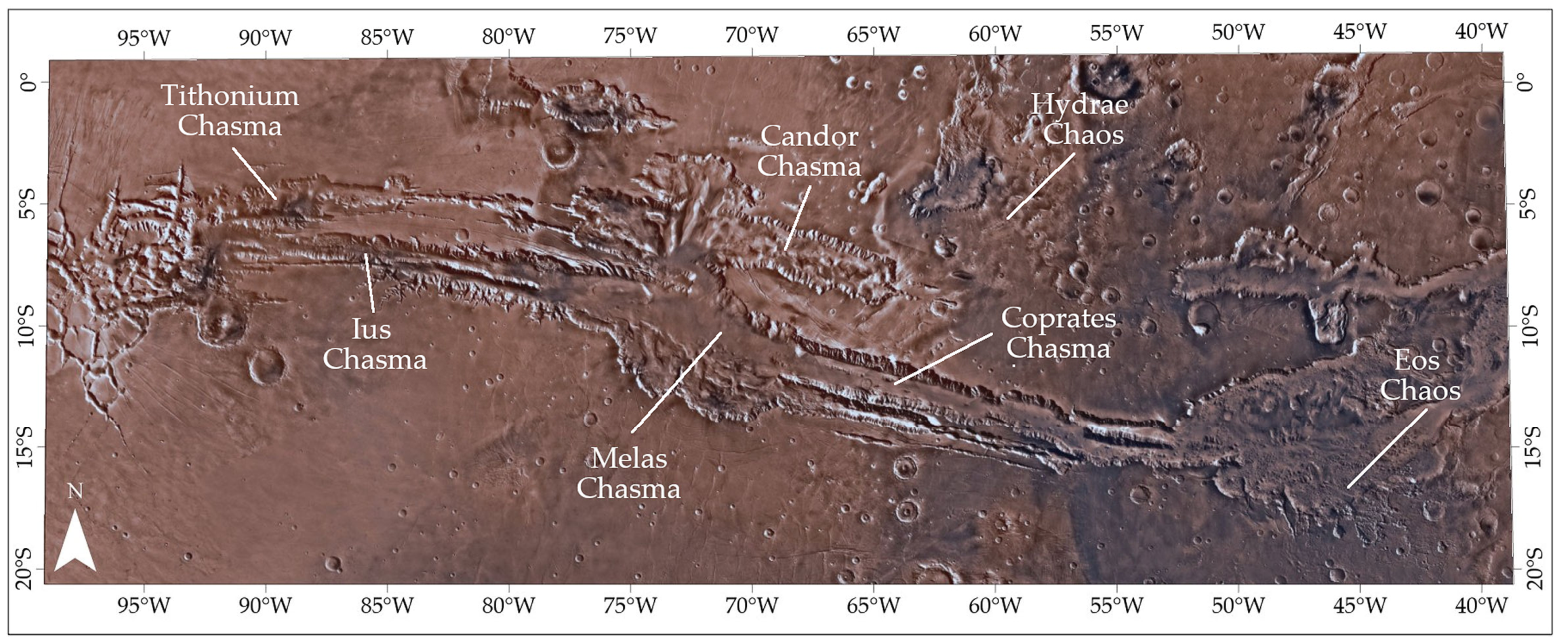
The study area is located within the Valles Marineris region, the largest canyon system on Mars and one of the most prominent tectono-geomorphological structures in the Solar System. Valles Marineris extends for more than 2000 km along the Martian equatorial zone and reaches widths of up to ~200 km, with maximum depths locally exceeding 9–10 km [37]. The canyon system comprises a series of interconnected troughs, including Ius, Tithonium, Ophir, Candor, Melas, and Coprates Chasmata, forming a structurally complex network of steep escarpments, fault-bounded basins, and chaos terrains (Figure 2).

The origin and evolution of Valles Marineris are widely attributed to large-scale extensional tectonics associated with lithospheric stretching and the uplift of the Tharsis volcanic province, followed by progressive faulting, collapse, and erosional modification of the initial graben structures [38,39]. Normal fault systems exert a strong control on canyon geometry and slope morphology, generating laterally continuous steep scarps and structurally conditioned slope breaks [40].

Mass-wasting processes are pervasive throughout the canyon system, and Valles Marineris hosts some of the largest landslide deposits identified on Mars. Extensive rock avalanches, rotational slumps, and debris-flow-like deposits have been documented along canyon margins, in some cases covering hundreds of kilometres and exhibiting complex emplacement morphologies [21]. These deposits represent key evidence of large-scale gravitational slope instability under Martian environmental conditions.

Geologically, Valles Marineris is characterised by a complex association of bedrock units, faulted wall sequences, chaotic terrains, and interior layered deposits, reflecting a long history of tectonic, volcanic, sedimentary, and erosional processes [41,42,43]. This heterogeneity produces strong contrasts in material properties and stratigraphic architecture, which may influence slope stability by favouring differential erosion, localised weakening, and the development of structurally controlled failure surfaces [44]. The occurrence of layered deposits and hydrated mineral phases in several chasmata further suggests that lithological variability and past alteration processes may have contributed to spatial differences in slope behaviour across the canyon system [45,46,47,48].

3. Materials and Methods

3.1. Landslide Inventory

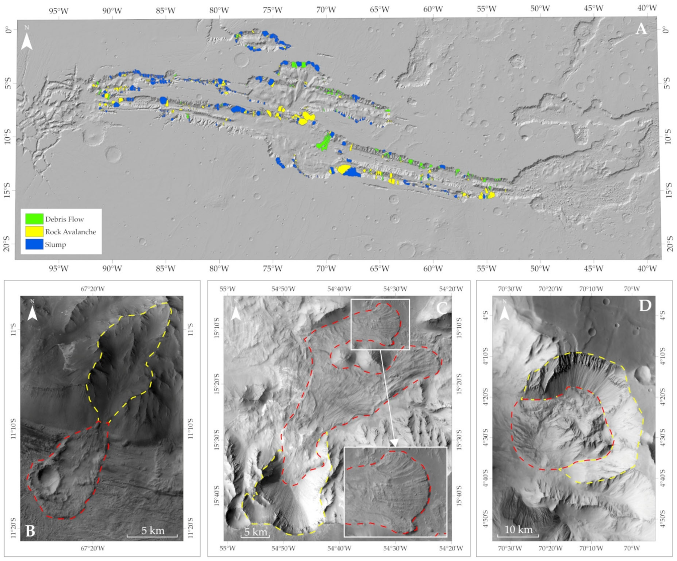
The landslide inventory adopted in this study is derived from the dataset published by Rajaneesh et al. [49] and consists of a total of 682 mapped landslides distributed along the canyon walls of the Valles Marineris system (Figure 3). The inventory includes different types of gravitational mass movements, reflecting the morphological and kinematic diversity of slope failures affecting the region. Specifically, the inventory is composed of 140 Debris Flows (Figure 3B), 251 Rock Avalanches (Figure 3C) and 291 Slumps (Figure 3D). For the purposes of landslide susceptibility modelling, the inventory was stratified according to landslide typology. Within each landslide type, the mapped features were initially randomly divided into training (60%) and testing datasets (40%). Subsequently, the allocation was manually refined to maximise the geographical separation between the two subsets. For each testing landslide, the minimum edge-to-edge distance to the nearest training polygon of the same landslide type was calculated. Polygons located in close proximity across the two subsets (i.e., neighbouring polygons or within a distance of a few kilometres) were reassigned or exchanged whenever possible, while preserving the approximately 60/40 training-to-testing proportion for each landslide category. The resulting final minimum edge-to-edge distances between training and testing polygons were 85 km for Debris Flows, 86 km for Rock Avalanches, and 60 km for Slumps. This procedure was adopted to reduce potential spatial dependence between calibration and validation data and to limit possible inflation of the AUC values caused by spatial leakage. The training datasets were used to develop susceptibility models for each landslide typology, whereas the testing datasets were reserved exclusively for model validation and predictive performance assessment.

Because the susceptibility model was developed using MOLA-derived conditioning factors, an additional raster-cell representation analysis was performed to evaluate whether the mapped landslide inventory is adequately represented at the spatial resolution of the MOLA DEM. For each mapped landslide polygon, the number of MOLA raster cells contained within its boundary was calculated. A diagnostic threshold of 30 MOLA cells was used to identify landslides potentially more sensitive to scale-related representation issues. Considering the MOLA cell size of approximately 463 m, 30 raster cells correspond to a surface of approximately 6.43 km². Therefore, landslides below this threshold were considered potentially more affected by raster generalisation, whereas landslides above this value were considered sufficiently represented for a regional-scale susceptibility analysis.

The results show that only 25 landslides, corresponding to 3.67% of the complete inventory, are represented by less than 30 MOLA cells. Conversely, 96.33% of the mapped landslides exceed this diagnostic threshold. Moreover, the median landslide size corresponds to 238 MOLA cells, with an interquartile range between 108 and 584 cells, indicating that a typical mapped landslide is represented by a substantial number of raster cells.

Descriptive statistics were also calculated separately for each landslide type to verify whether specific movement classes were more affected by scale-related representation issues. Debris Flows have a median size of 214 MOLA cells, with an interquartile range between 83 and 451 cells. Rock Avalanches show a median size of 168 MOLA cells, with an interquartile range between 73 and 463 cells. Slumps are generally larger, with a median size of 329 MOLA cells and an interquartile range between 168 and 776 cells. These values indicate that the typical landslide in each class is represented by a substantial number of raster cells and that even the lower quartile of each distribution is above a few-cell representation.

Moreover, only 6 Debris Flows, corresponding to 4.29% of the Debris Flow inventory, 15 Rock Avalanches, corresponding to 5.98% of the Rock Avalanche inventory, and 4 Slumps, corresponding to 1.37% of the Slump inventory, are represented by less than 30 MOLA cells. Given that landslides represented by less than 30 MOLA cells account for only 3.67% of the complete inventory, and that this proportion remains low for each landslide type, potential scale-related effects can be considered statistically negligible with respect to the overall inventory structure. Therefore, although local-scale geomorphic details may be smoothed by the MOLA DEM, the limited number of potentially under-represented landslides is unlikely to introduce systematic bias in the regional-scale susceptibility modelling. However, we must underline that the performed analysis does not evaluate the stability of the Frequency Ratio weights when using DEM at different spatial resolution. A dedicated multi-resolution analysis could therefore be developed as a separate future application to investigate the influence of DEM resolution on susceptibility patterns and factor rankings.

3.2. Predisposing Factors

Predisposing factors describe the topographic and geological conditions that favour slope instability and control the spatial distribution of landslides, independently of the triggering mechanism. In landslide susceptibility mapping, topographic factors are widely used to characterise the terrain conditions under which mass movements are more likely to occur and are commonly derived from Digital Elevation Models (DEMs) (e.g., [50]).

Regarding geology, lithology is widely recognised as an important factor controlling slope stability, as it influences rock strength, weathering processes, material cohesion, and the development of discontinuities. However, in this study, lithology and surface-material properties were not included as conditioning factors due to the lack of spatially continuous, homogeneous, and artefact-free datasets describing the lithological, compositional, or mechanical characteristics of the involved materials.

During the preliminary selection of predisposing factors, we considered the inclusion of THEMIS thermal inertia as an additional proxy for surface-material properties. In particular, we evaluated both the qualitative 8-bit and the quantitative 32-bit THEMIS thermal inertia products for their utilisation in distinguishing thermophysical surface classes, such as fine-grained dusty materials, sandy or weakly consolidated deposits, indurated surfaces, and rock-dominated or bedrock exposures. However, visual and spatial inspection of the THEMIS mosaic over the analysed Valles Marineris sector revealed relevant artefacts and inconsistencies, likely related to the acquisition and mosaicking process. These include abrupt discontinuities and artificial spatial patterns between adjacent mosaic tiles that compromise their use in susceptibility modelling. Representative examples of the no-data areas affecting the 8-bit product and the mosaic-related artefacts observed in the 32-bit product are provided in the Supplementary Materials (Figure S1). These issues could introduce artificial spatial patterns into the Frequency Ratio analysis and bias the resulting weights. For this reason, lithological, compositional, and material-property layers were not included in the final model, although their integration represents an important future development of the study.

The predisposing topographical factors used in this work were derived from the Mars Orbiter Laser Altimeter (MOLA) DEM, acquired by the Mars Global Surveyor (MGS) mission. MOLA DEM provides near-global topographic coverage of Mars and represents the most widely used dataset for regional-scale geomorphological analyses. The MOLA DEM used in this work has a spatial resolution of approximately 463 m at the equator and a vertical accuracy of a few metres, based on hundreds of millions of individual laser altimetry measurements [12]. The global MOLA dataset was spatially clipped to the extent of the Valles Marineris study area.

Based on the MOLA clipped DEM, three topographic predisposing factors were extracted using standard geomorphometric tools implemented in ESRI^TM ArcGIS Pro (3.6): Slope, Aspect, and Local Relief (as described below). These morphometric parameters represent key descriptors of terrain geometry and are widely recognised as primary controls on slope instability [51,52] since steep terrain combined with substantial elevation differences represent the basic morphological conditions required for landslide initiation.

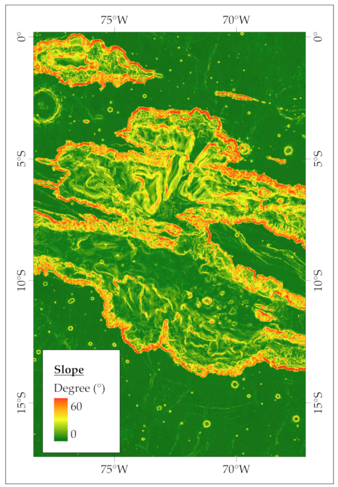
Slope (Figure 4) represents the dipping angle of the terrain surface, and it is one of the most fundamental controls on slope stability, as increasing slope angles enhance the gravitational driving forces acting on the material [53]. In the tectonically controlled environment of Valles Marineris, steep slopes are widespread along canyon walls and fault-related escarpments, making slope a key parameter for all the analysed landslide types.

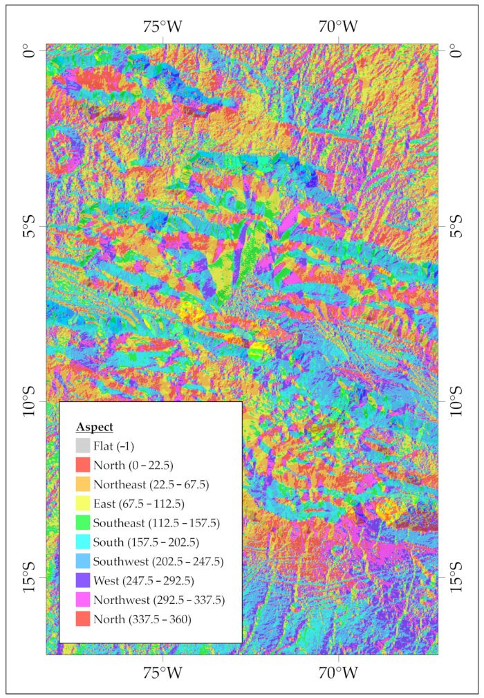
Aspect (Figure 5) describes the orientation of slopes towards North and provides information on the spatial arrangement of valley walls and the structural framework of the canyon system. Although aspect does not directly induce instability, it may influence landslide distribution by reflecting the geometric configuration of the terrain and the dominant orientations of structural lineaments.

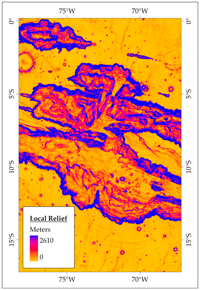
Local relief (Figure 6) represents a measure of relative topographic contrast. High values of local relief indicate the presence of large elevation differences over short horizontal distances, that are characteristic of deeply incised canyon systems such as Valles Marineris.

3.3. Triggering Factor

Triggering factors represent the external processes capable of initiating slope failure once favourable predisposing conditions are met. While predisposing factors define where landslides are more likely to occur, triggering factors control when instability is activated. On Mars, the identification of triggering mechanisms is inherently challenging due to the lack of direct observations and in situ measurements, and must therefore rely on indirect geomorphological and contextual evidence.

In Valles Marineris region, seismic shaking associated with tectonic activity is considered a plausible triggering mechanism due to the strong structural control of the canyon system, which is characterised by extensive networks of large extensional faults and kilometre-scale relief [38,39]. Since spatially continuous and reliable estimates of Peak Ground Acceleration (PGA) are not available for the study area, the direct incorporation of seismic loading into the landslide susceptibility modelling was prevented. For this reason, the potential influence of seismic shaking was represented using the distance from tectonic faults as a proxy variable. On Earth, distance to faults is commonly adopted in landslide susceptibility studies as an indirect indicator of seismic influence, under the assumption that areas closer to active or major fault systems are more likely to experience stronger seismic shaking and associated ground deformation (e.g., [54,55]).

This approach does not aim to quantify seismic ground motion or to associate individual landslides with specific seismic events. Rather, it provides a spatially based assessment of whether tectonically induced seismic shaking can be considered a coherent and physically reasonable trigger for the observed distribution of mass movements in Valles Marineris.

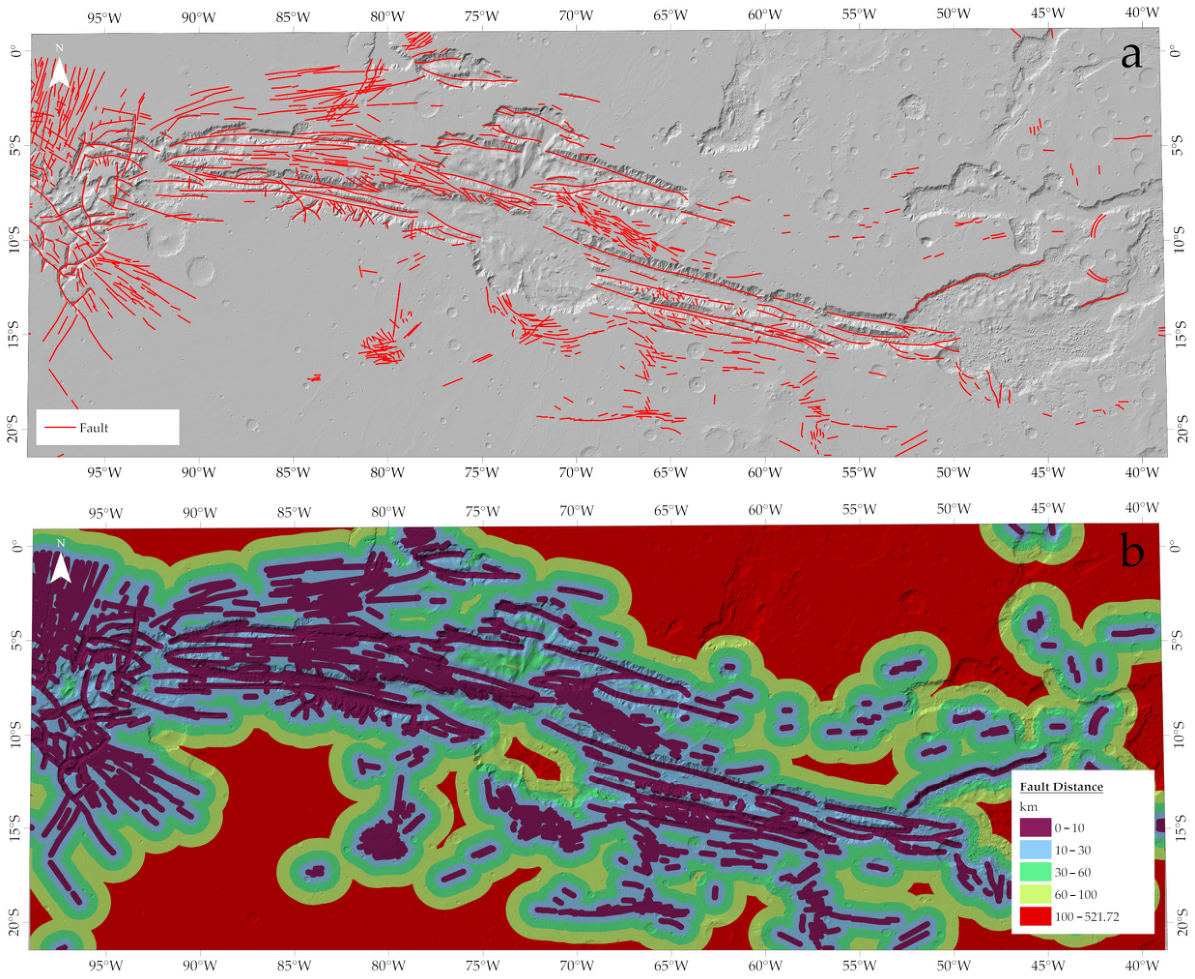
The fault network used in this study consists of major extensional structures mapped in the Valles Marineris region and was extracted from the structural dataset published by Knapmeyer et al. [56] (Figure 7a). These faults are interpreted as primary tectonic features related to the extensional evolution of the canyon system and are therefore considered appropriate for representing the spatial distribution of potential seismic sources.

Based on this faults dataset, a distance-to-fault raster layer was generated using the Euclidean distance tool implemented in ESRI^TM ArcGIS Pro (3.6) software. The resulting raster represents the horizontal distance between each cell of the study area and the nearest mapped fault segment, expressed in kilometres. The distance values were subsequently classified into five distance classes (0–10 km, 10–30 km, 30–60 km, 60–100 km, and >100 km) to evaluate the potential influence of tectonic structures on landslide occurrence (Figure 7b).

3.4. Assessment of Coupling Effects and Multicollinearity Among Conditioning Factors

Before developing the susceptibility model, the statistical relationships among the selected conditioning factors were evaluated to identify possible redundancy, multicollinearity, and coupling effects that would counter the basic assumptions of the Frequency Ratio method. Two complementary analyses were performed: Pearson’s correlation coefficient (r) was used to assess pairwise associations between conditioning factors and to identify possible coupling effects, whereas the Variance Inflation Factor (VIF) was calculated to evaluate multicollinearity.

Pearson’s correlation coefficient ranges from −1 to +1 and quantifies the strength and direction of the linear relationship between two variables. Values close to +1 indicate a strong positive correlation, while values close to −1 indicate a strong negative correlation; values close to 0 indicate weak or no linear correlation. In this study, the strength of correlation was interpreted using the following thresholds as reported in Yang et al. (2023) [57]: |r| < 0.3 indicates weak correlation, 0.30 ≤ |r| < 0.70 indicates moderate correlation, and |r| ≥ 0.70 indicates strong correlation. Therefore, only strongly correlated variables were considered potentially redundant or affected by relevant coupling effects, whereas weak to moderate correlations were interpreted as acceptable.

Two parameters, tolerance (TOL) and VIF, were used to quantify multicollinearity. The following Equations (1) and (2) are used to determine TOL and VIF for a given landslide conditioning factor:

$$TOL=1-{\mathrm{R}}^2$$

(1)

$$VIF={\displaystyle \frac{1}{(1-{\mathrm{R}}^2)}}$$

(2)

where R² is the coefficient of determination obtained by regressing the ith variable against all the remaining variables. According to Hamal et al. (2026) [58] a TOL value below 0.1 or a VIF above 10 indicates significant multicollinearity. The combined use of Pearson’s correlation matrix and VIF allowed both pairwise coupling and overall multicollinearity among the conditioning factors to be assessed before implementing the Frequency Ratio model.

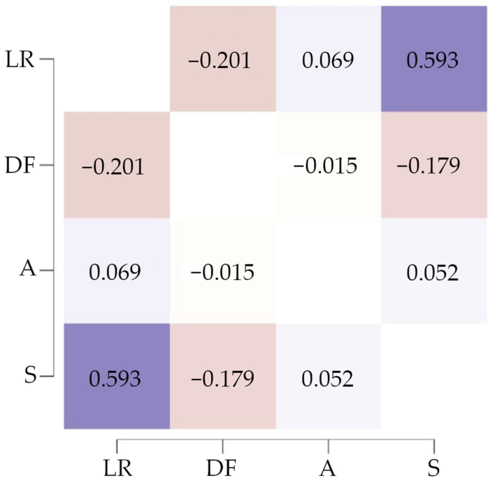
The Pearson correlation matrix and VIF/TOL results, presented in Figure 8 and

Table 1. Multicollinearity diagnostic results of conditioning factor.

Factor	TOL	VIF
Local relief	0.639	1.551
Slope	0.645	1.565
Distance from fault	0.647	1.546
Aspect	0.954	1.048

, indicate that no strong pairwise correlation (|r| ≥ 0.70) or severe multicollinearity (VIF > 10 or TOL < 0.1) occurs among the selected conditioning factors.

The highest Pearson’s correlation was observed between slope and local relief (r = 0.593), indicating a moderate positive correlation. This relationship is geomorphologically expected in Valles Marineris, where steep canyon walls are commonly associated with high elevation contrasts. However, the correlation remains below the adopted threshold for strong coupling and does not imply statistical redundancy. Slope and local relief were therefore retained in this analysis because they describe different physical controls: slope is directly related to the shear resistance, including the relationship between slope angle and internal friction angle [59], whereas local relief indicates the vertical elevation contrast of the terrain and can be interpreted as a proxy for the gravitational potential energy available for mass movement processes [60].

3.5. Frequency Ratio (FR) Method

Landslide susceptibility was assessed using the Frequency Ratio (FR) method, a bivariate statistical approach widely employed to quantify the spatial relationship between landslide occurrence and conditioning factors [61].

Prior to model implementation, the triggering-related factor were rasterised, co-registered, and resampled to a common raster resolution consistent with the MOLA DEM, ensuring spatial consistency among datasets. Each factor was then classified into discrete classes to enable the computation of class-specific landslide frequencies. The classes used for each predisposing and triggering-related factor are reported in

Table 2. Discrete classes defined for each predisposing and triggering-related factor used to compute class-specific landslide frequencies in the Frequency Ratio analysis.

Factor	Class
Slope (°)	0–10
	10–20
	20–30
	30–40
	40–50
	50–60
Aspect	Flat (−1)
	North (0–22.5°)
	Northeast (22.5–67.5°)
	East (67.5–112.5°)
	Southeast (112.5–157.5°)
	South (157.5–202.5°)
	Southwest (202.5–247.5°)
	West (247.5–292.5°)
	Northwest (292.5–337.5°)
	North (337.5–360°)
Local Relief (m)	0
	150
	400
	800
	>1500
Distance from Fault (km)	0–10
	10–30
	30–60
	60–100
	100–520

.

For each landslide type, FR values were computed independently using the training subset of the landslide inventory, in order to avoid information leakage and ensure an objective evaluation of model performance. This separation allows the validation dataset to remain fully independent from the model calibration phase.

The FR for a given class i was calculated as shown in Equation (3):

$$F{R}_i={\displaystyle \frac{\left(\frac{A_{L,i}}{A_L}\right)}{\left(\frac{A_{C,i}}{A_C}\right)}}$$

(3)

where A_L,i is the landslide area falling within class i of predisposing and triggering factors, A_L is the total landslide area in the training dataset, A_C,i is the area of class i of predisposing and triggering factors, and A_C is the total study area. FR values greater than 1 indicate that landslides occupy a larger proportion of area in that class than expected under a random spatial distribution, suggesting a positive association, whereas FR values lower than 1 indicate a negative association.

To combine the influence of multiple predisposing and triggering-related factors into a single susceptibility measure, FR values were subsequently log-transformed to obtain a class-specific weight (W_C), defined as Equation (4):

$$W_c=\ln \left(FR\right)$$

(4)

This transformation converts the inherently multiplicative nature of FR into an additive weighting scheme, allowing the contributions of different factor classes to be summed in a mathematically consistent way. The use of W_C also reduces the influence of extreme FR values, improves numerical stability, and facilitates the interpretation of factor effects. Positive W_C values indicate factor classes that increase the likelihood of landslide occurrence, whereas negative values indicate classes that decrease it, providing a direct quantitative measure of the relative contribution of each class to overall landslide susceptibility.

The Landslide Susceptibility Index (LSI) for each raster cell was then computed by summing the W_C values associated with the corresponding factor classes as shown in Equation (5):

$$LSI=\sum _{j=1}^n{W}_{c,j}=\sum _{j=1}^n\ln \left(F{R}_j\right)$$

(5)

where W_C,j represents the weight coefficient associated with the class of the $j$th factor, FR_j is the frequency ratio value of that class, and n is the total number of predisposing and triggering factors considered in the model.

The resulting LSI represents a continuous numerical variable expressing the relative likelihood of landslide occurrence at the pixel level, with highest values indicating greatest susceptibility. Since separate FR models have been developed for rock avalanches, landslides, and debris flows, each LSI expresses the relative propensity for that specific landslide type to occur based on its relationships with the conditioning factors. Accordingly, LSI values should be interpreted only within the respective type-specific map and should not be directly compared across the three models; a given LSI value should not be interpreted as a diagnostic threshold for distinguishing slumps, rock avalanches, and debris flows.

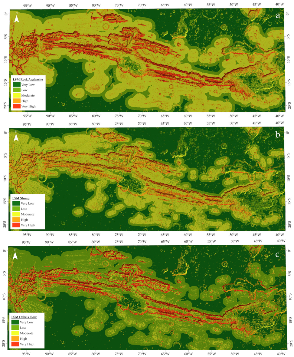
The continuous LSI raster was subsequently normalised and classified into discrete susceptibility classes (e.g., very low, low, moderate, high, and very high) to produce the final Landslide Susceptibility Map (LSM). In this framework, the LSI represents the quantitative type-specific output of the Frequency Ratio model, whereas the LSM is the categorical and spatial representation of that index, allowing an intuitive visual interpretation of susceptibility patterns and a direct comparison with the spatial distribution of mapped landslides.

Separate LSMs were generated for Rock Avalanches, Slumps and Debris Flows, enabling a type-specific evaluation of susceptibility.

3.6. Accuracy Assessment

The predictive performance of the LSMs was evaluated using testing datasets and a Prediction Rate Curve approach.

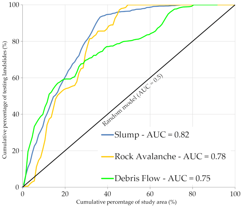
The Prediction Rate Curve (PRC) was constructed by plotting the cumulative proportion of validation landslides (Y) against the cumulative proportion of the study area (X), with susceptibility ranks ordered from highest to lowest. A model with strong predictive performance is expected to concentrate a large fraction of landslides within a relatively small portion of the total area, producing a curve that departs markedly from the diagonal corresponding to random prediction.

Model accuracy was quantified by computing the Area Under the Curve (AUC) using the trapezoidal method as shown in Equation (6):

$$AUC=\sum _{i=1}^{N-1}\left(X_{i+1}-X_i\right)\hspace{0.17em}{\displaystyle \frac{Y_{i+1}+Y_i}{2}}$$

(6)

AUC values range from 0.5 (no predictive skill) to 1.0 (perfect prediction), with higher values indicating a greater ability of the susceptibility model to correctly rank landslide-prone areas. Accuracy metrics were computed separately for all the movement type, enabling a comparative evaluation of predictive performance across different landslide mechanisms.

4. Results

The results of the FR analysis for Rock Avalanches, Slumps and Debris Flows are summarised in

Table 3. Results of the FR analysis for Rock Avalanches. Landslide area (A_L); Class area (A_C); Frequency Ratio (FR); class-specific weight (Wc); (-) not applicable.

Rock Avalanche
Factor	Class	AL (m2)	AC (m2)	FR	Wc
Slope (°)	0–10	6,335,233,713	4,259,044,062,473	0.46	−0.77
	10–20	4,352,805,886	355,159,270,654	3.80	1.34
	20–30	4,110,899,937	219,006,873,315	5.83	1.76
	30–40	868,116,383	30,448,115,284	8.85	2.18
	40–50	4,932,479	161,419,857	9.48	2.25
	50–60	0	12,647,771	-	-
Total		15,671,988,399	4,863,832,389,354
Aspect	Flat (−1)	0	0	-	-
	North (0–22.5°)	1,213,818,856	308,064,545,044	1.22	0.20
	Northeast (22.5–67.5°)	2,028,106,876	695,525,794,094	0.90	−0.10
	East (67.5–112.5°)	1,393,103,761	736,900,940,415	0.59	−0.53
	Southeast (112.5–157.5°)	1,772,904,679	735,885,474,462	0.75	−0.29
	South (157.5–202.5°)	3,466,675,230	658,523,561,004	1.63	0.49
	Southwest (202.5–247.5°)	2,458,090,411	501,532,781,913	1.52	0.42
	West (247.5–292.5°)	855,249,045	472,699,937,044	0.56	−0.58
	Northwest (292.5–337.5°)	1,314,398,545	513,473,135,213	0.79	−0.23
	North (337.5–360°)	1,169,640,996	241,226,220,165	1.50	0.41
Total		15,671,988,399	4,863,832,389,354
Local Relief (m)	0	1,982,856,739	3,667,908,897,202	0.17	−1.79
	150	4,062,861,877	580,330,967,671	2.17	0.78
	400	4,444,378,439	364,120,966,699	3.79	1.33
	800	4,967,435,717	245,807,714,433	6.27	1.84
	>1500	214,455,628	5,663,843,349	11.75	2.46
Total		15,671,988,399	4,863,832,389,354
Distance from Fault (km)	0–10	9,637,207,021	979,019,149,989	3.06	1.12
	10–30	4,524,155,933	951,192,553,206	1.48	0.39
	30–60	1,352,357,192	843,604,825,117	0.50	−0.70
	60–100	158,268,254	766,420,409,191	0.06	−2.75
	100–520	0	1,323,595,451,851	-	-
Total		15,671,988,399	4,863,832,389,354

,

Table 4. Results of the FR analysis for Slumps.

Slump
Factor	Class	AL (m2)	AC (m2)	FR	Wc
Slope (°)	0–10	9,225,881,126	4,259,044,062,473	0.30	−1.19
	10–20	7,487,289,348	355,159,270,654	3.73	1.32
	20–30	7,653,921,371	219,006,873,315	6.05	1.80
	30–40	3,712,012,469	30,448,115,284	21.09	3.05
	40–50	34,956,267	161,419,857	37.46	3.62
	50–60	0	0	-	-
Total		28,114,060,582	4,863,832,389,354
Aspect	Flat (−1)	0	0	-	-
	North (0–22.5°)	2,135,334,690	308,064,545,044	1.20	0.18
	Northeast (22.5–67.5°)	3,484,689,503	695,525,794,094	0.87	−0.14
	East (67.5–112.5°)	2,125,469,731	736,900,940,415	0.50	−0.70
	Southeast (112.5–157.5°)	3,087,732,135	735,885,474,462	0.73	−0.32
	South (157.5–202.5°)	6,151,659,696	658,523,561,004	1.62	0.48
	Southwest (202.5–247.5°)	4,941,272,130	501,532,781,913	1.70	0.53
	West (247.5–292.5°)	2,395,898,279	472,699,937,044	0.88	−0.13
	Northwest (292.5–337.5°)	2,146,915,294	513,473,135,213	0.72	−0.32
	North (337.5–360°)	1,645,089,124	241,226,220,165	1.18	0.17
Total		28,114,060,582	4,863,832,389,354
Local Relief (m)	0	1,373,588,299	3,667,908,897,202	0.06	−2.74
	150	7,298,353,940	580,330,967,671	2.18	0.78
	400	7,713,754,492	364,120,966,699	3.67	1.30
	800	10,531,272,535	245,807,714,433	7.41	2.00
	>1500	1,197,091,317	5,663,843,349	36.57	3.60
Total		28,114,060,582	4,863,832,389,354
Distance from Fault (km)	0–10	13,234,485,729	979,019,149,989	2.34	0.85
	10–30	12,878,918,297	951,192,553,206	2.34	0.85
	30–60	1,969,560,490	843,604,825,117	0.40	−0.91
	60–100	31,096,066	766,420,409,191	0.01	−4.96
	100–520	0	1,323,595,451,851	-	-
Total		28,114,060,582	4,863,832,389,354

and

Table 5. Results of the FR analysis for Debris Flows.

Debris Flow
Factor	Class	AL (m2)	AC (m2)	FR	Wc
Slope (°)	0–10	2,755,969,278	4,259,044,062,473	0.39	−0.95
	10–20	1,965,914,744	355,159,270,654	3.30	1.19
	20–30	2,972,569,463	219,006,873,315	8.10	2.09
	30–40	457,219,399	30,448,115,284	8.96	2.19
	40–50	857,823	161,419,857	3.17	1.15
	50–60	0	12,647,771	-	-
Total		8,152,530,707	4,863,832,389,354
Aspect	Flat (−1)	0	0	-	-
	North (0–22.5°)	251,341,996	308,064,545,044	0.49	−0.72
	Northeast (22.5–67.5°)	499,896,069	695,525,794,094	0.43	−0.85
	East (67.5–112.5°)	516,623,608	736,900,940,415	0.42	−0.87
	Southeast (112.5–157.5°)	1,046,543,466	735,885,474,462	0.85	−0.16
	South (157.5–202.5°)	2,454,015,754	658,523,561,004	2.22	0.80
	Southwest (202.5–247.5°)	1,858,686,930	501,532,781,913	2.21	0.79
	West (247.5–292.5°)	762,818,670	472,699,937,044	0.96	−0.04
	Northwest (292.5–337.5°)	530,777,680	513,473,135,213	0.62	−0.48
	North (337.5–360°)	231,826,534	241,226,220,165	0.57	−0.56
Total		8,152,530,707	4,863,832,389,354
Local Relief (m)	0	1,327,051,427	3,667,908,897,202	0.22	−1.53
	150	1,271,292,964	580,330,967,671	1.31	0.27
	400	1,927,527,186	364,120,966,699	3.16	1.15
	800	3,553,744,215	245,807,714,433	8.63	2.15
	>1500	72,914,914	5,663,843,349	7.68	2.04
Total		8,152,530,707	4,863,832,389,354
Distance from Fault (km)	0–10	4,295,117,322	979,019,149,989	2.62	0.96
	10–30	3,199,463,517	951,192,553,206	2.01	0.70
	30–60	645,296,985	843,604,825,117	0.46	−0.78
	60–100	12,652,882	766,420,409,191	0.01	−4.62
	100–520	0	1,323,595,451,851	-	-
Total		8,152,530,707	4,863,832,389,354

which reports, for each predisposing and triggering factor class, the landslide area (A_L), class area (A_C), Frequency Ratio (FR) values, and the associated class-specific weight (Wc) used in the susceptibility model.

Figure 9 presents the Landslide Susceptibility Maps (LSMs) for Rock Avalanches, Slumps, and Debris Flows in the Valles Marineris region. Across all three maps, susceptibility values display a marked spatial variability, with high and very high susceptibility classes predominantly concentrated along the main canyon system and its steep marginal slopes. Lower susceptibility classes are mainly distributed across smoother plateaus and gently sloping terrains.

The predictive performance of the landslide susceptibility models was evaluated using PRCs and the corresponding AUC values derived from the independent testing dataset (Figure 10). All three models exhibit prediction curves well above the random prediction line, indicating a clear ability to discriminate areas with the greater probability of landslide occurrence.

The slump susceptibility model shows the highest predictive performance, with an AUC of 0.82, followed by the rock avalanche model (AUC = 0.78) and the debris flow model (AUC = 0.75). The PRCs indicate that a substantial proportion of validation landslides is captured within a relatively small fraction of the study area ranked as highly susceptible, with the slump model displaying the steepest initial curve and the debris flow model showing a more gradual cumulative trend. Overall, the AUC values indicate good predictive capability for all three landslide types.

5. Discussion

The application of the FR method to the landslide inventory of Valles Marineris provides quantitative insights into the geomorphological and structural factors governing slope instability on Mars. The susceptibility models developed for the three analysed landslide types show good predictive capability, with AUC values of 0.82 for slumps, 0.78 for rock avalanches and 0.75 for debris flows, indicating that the adopted statistical framework effectively discriminates between areas characterised by different probabilities of landslide occurrence. These values fall within the range generally considered indicative of good model performance in landslide susceptibility studies [51].

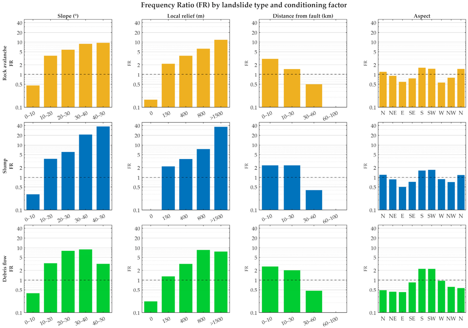
The analysis of the FR values highlights the dominant role of morphometric parameters, particularly slope gradient and local relief. High FR values are consistently associated with steeper slope classes. For example, slope classes between 30° and 40° show FR values of 21.09 for slumps and 8.96 for debris flows, while the steepest slope classes (40–50°) reach FR values up to 37.46 for slumps, indicating a very strong positive contribution of these classes to landslide susceptibility. Such results confirm that slope gradient represents a key conditioning factor controlling gravitational instability. A synthetic overview of the relationships between the analysed predisposing and triggering factors on the three landslide types is provided in Figure 11, which summarises the FR values for each class and factor. The patterns are expected, because slope gradient and topographic relief represent fundamental geomorphological conditions for the occurrence of mass movements, since gravitational slope failures cannot develop in the absence of sufficiently steep slopes and significant elevation contrasts. Similar observations have been reported in numerous landslide susceptibility studies, where morphometric parameters often dominate statistical models because they directly control the balance between driving and resisting forces acting on hillslopes [62,63].

Despite this general behaviour, the results reveal distinct geomorphological controls for different landslide types. Rock avalanches show the strongest association with areas characterised by high local relief. In particular, the class exceeding 1500 m of local relief shows FR values of 11.75, indicating a strong positive relationship between large elevation differences and rock avalanche occurrence. This pattern suggests that large elevation contrasts provide the gravitational potential energy required to sustain large failures. Similar relationships between large-scale rock slope failures and high-relief topography have been widely documented in terrestrial mountain environments [64].

Slumps, on the other hand, appear to be primarily controlled by slope gradient, with the steepest slope classes showing the highest FR values. The maximum value observed for this parameter (FR = 37.46) indicates a very strong concentration of slump events in steep versants, reflecting the mechanics of rotational failures that typically develop where gravitational stresses exceed the shear strength of the material. Debris flows show an intermediate behaviour, with high FR values associated with both steep slopes and elevated local relief. For example, local relief classes around 800 m show FR values exceeding 8, indicating that these processes require both sufficient slope steepness and adequate topographic energy to mobilise unconsolidated material.

Beyond these dominant morphometric controls, the analysis of distance from faults provides additional insights into the possible role of geo-structural factors in landslide occurrence. The FR values show a clear decrease with increasing distance from major fault systems. For instance, areas located within 0–10 km from faults show FR values of 3.06 for rock avalanches and 2.62 for debris flows, while values decrease markedly at greater distances. Although the contribution of this parameter is lower than that of slope gradient and local relief, this pattern suggests that proximity to tectonic structures may increase the likelihood of landslide occurrence. Fault zones are typically characterised by increased rock fracturing and reduced rock mass strength, conditions that can facilitate gravitational slope failures. In addition, proximity to tectonic structures may indicate areas where seismic shaking could act as a triggering mechanism for landslides, as widely documented in terrestrial environments [65]. In the tectonically complex setting of Valles Marineris, where tectonic processes played a major role in the formation and evolution of the canyon system, this relationship may reflect the influence of structurally weakened rock masses or past seismic activity associated with regional stress fields [66]. From this perspective, distance from faults may represent a useful additional indicator for identifying areas where seismically induced landslides could potentially occur, complementing the dominant morphometric controls highlighted by the susceptibility analysis.

A useful comparison can be made with the global-scale study of Martian landslides conducted by Roback & Ehlmann [27], where landslide occurrence was investigated using deterministic slope stability modelling with the Scoops3D software (https://www.usgs.gov/software/scoops3d, accessed on 26 June 2026). Their results demonstrated that landslide distribution on Mars cannot be explained solely by the presence of steep slopes and highlighted the importance of geological and tectonic factors. Although the methodological approach adopted in the present study differs substantially, relying on a statistical susceptibility framework rather than deterministic modelling, both studies emphasise the importance of the interaction between topographic and structural factors in controlling landslide occurrence on Mars. In this context, the FR-based approach here presented provides a complementary perspective by quantifying the relative influence of different conditioning parameters and by enabling a direct comparison between different types of mass movements.

Finally, aspect appears to exert only a minor influence on landslide occurrence, as indicated by FR values generally close to unity across the analysed classes. This behaviour suggests that slope dip direction does not significantly control the spatial distribution of mass movements at the regional scale considered in this study, a result consistent with many susceptibility analyses where aspect shows weaker correlations with landslide occurrence compared with morphometric variables [51]. The limited contribution of aspect to the susceptibility models is also relevant for interpreting the possible role of climatic or volatile-related controls. Since volatile stability and insolation-driven processes are expected to exhibit some degree of aspect dependence, particularly in relation to gully evolution [67] and Recurring Slope Lineae (RSL) activity [68], the absence of a strong aspect bias suggests that such factors are unlikely to represent the primary control on the spatial distribution of the mapped landslides in Valles Marineris.

Future developments of this research could further improve the reliability and predictive capability of the susceptibility analysis by integrating additional datasets and more advanced modelling approaches.

First, the use of a higher-resolution DEM could significantly enhance the accuracy of morphometric parameters such as slope gradient and local relief, which have been identified as the most influential conditioning factors in the present study. Moreover, higher-resolution topographic data would allow the inclusion of additional terrain attributes, such as surface roughness, planform and profile curvature, multi-scale Topographic Position Index (TPI), and slope metrics calculated at different spatial scales. These parameters could provide a more detailed representation of local morphology and slope complexity, potentially improving the robustness and spatial reliability of analysis at different type of scale. In fact, beyond improving the spatial resolution of susceptibility models, higher-resolution topographic datasets could also provide an important bridge between regional-scale remote sensing analyses and theoretical or experimental studies of slope stability under reduced-gravity conditions. In particular, recent theoretical and laboratory investigations have shown that gravity can influence both the maximum angle of stability and the post-avalanche relaxation angle of granular materials in planetary environments [69,70]. Therefore, detailed morphometric information derived from high-resolution DEMs, including slope distributions, local relief, roughness, and curvature metrics, could help translate particle-scale and laboratory-derived predictions into spatially explicit susceptibility assessments. This integration would allow planetary landslide susceptibility mapping to move beyond purely empirical terrain-factor correlations, contributing to a more physically grounded understanding of mass movement processes across different gravitational regimes.

However, the adoption of higher-resolution topographic data should be accompanied by careful direct inspection and correction of potential artefacts, which may otherwise propagate into derived geomorphometric products and affect the reliability of susceptibility modelling. In this regard, future cleaned DEM products, potentially obtained combining stereo-photogrammetry and photoclinometry, or new laser altimetry datasets from future missions, could provide more robust topographic constraints for landslide susceptibility analyses. As an example, during the preliminary phase of the analysis, a higher-resolution DEM derived from High Resolution Stereo Camera (HRSC) stereo imagery [71], specifically the product generated by Tao et al. [72], was tested. As also acknowledged by the authors [72], the dataset may contain local interpolation artefacts and topographic inconsistencies. Such artefacts could introduce spurious morphometric patterns and generate statistical outliers, potentially biasing the relationships between landslide occurrence and predisposing factors. For this reason, the HRSC-derived DEM was not adopted in the final susceptibility modelling. Despite its moderate spatial resolution, the MOLA DEM clipped to the study area is considered appropriate for the purposes of this study. Landslides in Valles Marineris typically involve large source areas and extensive runout zones, with spatial dimensions significantly larger than a single MOLA pixel [20,21]. Consequently, the selected DEM was considered sufficiently descriptive of the topographic conditions and permitted to avoid scale-related issues linked to the representation of events whose dimensions are smaller than the MOLA DEM pixel size.

Secondly, further improvement would involve the inclusion of detailed lithological and surface-material information. Lithology is widely recognised as important controls on slope stability, influencing rock strength, weathering processes and the development of discontinuities. The integration of a detailed geological layer could therefore provide additional explanatory power for the spatial distribution of the different types of mass movements analysed in this study. Although several datasets potentially useful for this purpose are available for Mars, including hyperspectral products and thermal inertia data, their direct integration into the present regional-scale Frequency Ratio workflow is limited by issues related to spatial continuity, heterogeneous resolution, variable data quality, and possible mosaic-related artefacts.

On Mars, geological mapping is commonly achieved through the combined analysis of morphology, stratigraphic relationships, and mineralogical composition derived from hyperspectral datasets. In particular, the use of instruments such as the Compact Reconnaissance Imaging Spectrometer for Mars (CRISM) enable the identification and spatial mapping of surface minerals based on their diagnostic spectral signatures, providing key constraints on lithology and alteration processes [73,74,75]. The resulting mineralogical maps can be used to delineate geologic units and refine geological maps, which can then be integrated into susceptibility analyses to better constrain the spatial variability of slope processes. However, the footprint of current hyperspectral datasets does not fully cover the study area, limiting the completeness of geological mapping. This emphasises the need for future hyperspectral missions with broader, ideally global, coverage to support more comprehensive geological interpretation processes.

In addition, thermal inertia data derived from the Thermal Emission Imaging System (THEMIS) [76] may represent a valuable proxy for surface-material properties. Thermal inertia is sensitive to particle size, rock abundance, induration, and the degree of surface consolidation, and can therefore help to distinguish between competent bedrock, coarse blocky surfaces, sandy deposits, and loose unconsolidated materials [77]. Its integration into landslide susceptibility modelling could improve the interpretation of material-dependent controls on slope instability.

However, as already presented in the Materials and Methods chapter, for the present regional-scale analysis of Valles Marineris, the available thermal inertia products were not included in the final model because they are affected by spatial discontinuities, mosaicking artefacts, and inconsistencies. These issues could only introduce artificial spatial patterns into the Frequency Ratio analysis and bias the resulting weights. For this reason, THEMIS-derived thermal inertia data is considered an important future development, provided that spatially continuous, homogeneous, and artefact-free products become available at an appropriate scale for susceptibility modelling.

Finally, future work could explore the application of more advanced machine learning algorithms for susceptibility modelling. While the Frequency Ratio approach adopted here provides a transparent, widely used and robust statistical framework, recent studies have shown that more advanced machine learning algorithms can capture complex nonlinear relationships between conditioning factors and landslide occurrence, often resulting in improved predictive performance [78]. Among the most widely applied methods, Random Forest (RF) [79], Support Vector Machines (SVM) [80], Artificial Neural Networks (ANN) [81], and, more recently, Convolutional Neural Networks (CNN) [82] could be tested for landslide susceptibility mapping in planetary environments. These approaches are increasingly used in landslide susceptibility studies on Earth due to their ability to model complex nonlinear interactions among conditioning factors [83,84]. The comparison between traditional statistical approaches and machine learning techniques could therefore represent a promising direction for refining the susceptibility assessment.

Nevertheless, future improvements in Martian landslide susceptibility modelling are expected to depend first on the availability of reliable input datasets and only subsequently on the adoption of more complex predictive algorithms. More advanced Machine Learning and Deep Learning models would be meaningful only if supported by more detailed, spatially continuous, and homogeneous data, including higher-resolution topography, improved lithological or surface-material information, and larger polygonal landslide inventories.

6. Conclusions

The application of the Frequency Ratio method provides a quantitative and spatially explicit assessment of landslide susceptibility in Valles Marineris, extending a predictive modelling framework widely used in terrestrial geomorphology to a Martian regional context. The main contribution of this study is not simply the identification of slope gradient as a controlling factor, which is expected from geomorphological and geotechnical principles, but the demonstration that a terrestrial-style susceptibility approach can reproduce coherent and independently validated patterns of landslide distribution on Mars.

The results show that the model can differentiate the spatial susceptibility patterns of different landslide types. Independent validation yielded AUC values of 0.75 for Debris Flows, 0.78 for Rock Avalanches, and 0.82 for Slumps, indicating that the predictive performance varies according to landslide typology. This type-dependent behaviour suggests that the mapped instability patterns are not controlled by a single generic topographic condition, but by different combinations of morphometric and structural factors.

At the regional scale imposed by the MOLA DEM, slope gradient and local relief emerge as the dominant morphometric controls on landslide susceptibility. Their influence is consistent with the expected role of gravitational stress, slope steepness, and topographic energy in promoting mass waste under Martian environmental conditions. Distance from faults shows a weaker but still meaningful contribution, suggesting that structural discontinuities may act as secondary pre-conditioning elements rather than as primary control on landslide occurrence across the whole study area.

Overall, these results support the use of statistical landslide susceptibility mapping as a valuable tool for planetary geomorphology. By producing type-specific susceptibility maps for Valles Marineris and quantitatively evaluating the relative role of morphometric and structural controls, this study contributes to bridging the methodological gap between terrestrial hazard-oriented approaches and the analysis of extra-terrestrial landscapes.

References

1. Esposito, G.; Salvini, R.; Matano, F.; Sacchi, M.; Danzi, M.; Somma, R.; Troise, C. Multitemporal monitoring of a coastal landslide through SfM-derived point cloud comparison. Photogramm. Rec. 2017, 32, 459–479. [Google Scholar] [CrossRef]
2. Casagli, N.; Intrieri, E.; Tofani, V.; Gigli, G.; Raspini, F. Landslide detection, monitoring and prediction with remote-sensing techniques. Nat. Rev. Earth Environ. 2023, 4, 51–64. [Google Scholar] [CrossRef]
3. Kumar, P.S.; Xiao, Z.; Wagner, R.; Zhao, J. Gullies and landslides on the Moon: Evidence for dry-granular flows. J. Geophys. Res. Planets 2013, 118, 206–223. [Google Scholar] [CrossRef]
4. Scaioni, M.; Yordanov, V.; Brunetti, M.T.; Melis, M.T.; Zinzi, A.; Kang, Z.; Giommi, P. Recognition of landslides in lunar impact craters. Eur. J. Remote Sens. 2018, 51, 47–61. [Google Scholar] [CrossRef]
5. Ermini, A.; Salvini, R.; Marrocchesi, P.S. Landslide susceptibility mapping in lunar south pole region. In Proceedings of the 24th International Multidisciplinary Scientific GeoConference SGEM 2024, Albena, Bulgaria, 29 June–8 July 2024; Volume 6.1, pp. 459–466. [Google Scholar] [CrossRef]
6. McEwen, A.S. Mobility of large rock avalanches: Evidence from Valles Marineris, Mars. Geology 1989, 17, 1111–1114. [Google Scholar] [CrossRef]
7. Magnarini, G.; Mitchell, T.M.; Grindrod, P.M.; Goren, L.; Schmitt, H.H. Longitudinal ridges imparted by high-speed granular flow mechanisms in martian landslides. Nat. Commun. 2019, 10, 4711. [Google Scholar] [CrossRef] [PubMed]
8. Brunetti, M.T.; Xiao, Z.; Komatsu, G.; Peruccacci, S.; Guzzetti, F. Large rock slides in impact craters on the Moon and Mercury. Icarus 2015, 260, 289–300. [Google Scholar] [CrossRef]
9. Irion, R. Landslide exposes roots of Io’s peaks. Science 1998, 279, 1457. [Google Scholar] [CrossRef]
10. Singer, K.N.; McKinnon, W.B.; Schenk, P.M.; Moore, J.M. Massive ice avalanches on Iapetus mobilized by friction reduction during flash heating. Nat. Geosci. 2012, 5, 574–578. [Google Scholar] [CrossRef]
11. Mutch, T.A.; Binder, A.B.; Huck, F.O.; Levinthal, E.C.; Liebes, S.; Morris, E.C.; Patterson, W.R.; Pollack, J.B.; Sagan, C.; Taylor, G.R. The surface of Mars: Their view from the Viking 1 lander. Science 1976, 193, 791–801. [Google Scholar] [CrossRef] [PubMed]
12. Smith, D.E.; Zuber, M.T.; Frey, H.V.; Garvin, J.B.; Head, J.W.; Muhleman, D.O.; Pettengill, G.H.; Phillips, R.J.; Solomon, S.C.; Zwally, H.J.; et al. Mars Orbiter Laser Altimeter: Experiment summary after the first year of global mapping of Mars. J. Geophys. Res. Planets 2001, 106, 23689–23722. [Google Scholar] [CrossRef]
13. McEwen, A.S.; Eliason, E.M.; Bergstrom, J.W.; Bridges, N.T.; Hansen, C.J.; Delamere, W.A.; Grant, J.A.; Gulick, V.C.; Herkenhoff, K.E.; Keszthelyi, L.; et al. Mars Reconnaissance Orbiter’s High Resolution Imaging Science Experiment (HiRISE). J. Geophys. Res. Planets 2007, 112, E05S02. [Google Scholar] [CrossRef]
14. Malin, M.C.; Bell, J.F.; Cantor, B.A.; Caplinger, M.A.; Calvin, W.M.; Clancy, R.T.; Edgett, K.S.; Edwards, L.; Haberle, R.M.; James, P.B.; et al. Context Camera investigation on board the Mars Reconnaissance Orbiter. J. Geophys. Res. Planets 2007, 112, E05S04. [Google Scholar] [CrossRef]
15. Lucchitta, B.K. A large landslide on Mars. Geol. Soc. Am. Bull. 1978, 89, 1601–1609. [Google Scholar] [CrossRef]
16. Lucas, A.; Mangeney, A. Mobility and topographic effects for large Valles Marineris landslides on Mars. Geophys. Res. Lett. 2007, 34, L10201. [Google Scholar] [CrossRef]
17. Barzegar, Y.; Biglari, M.; Ghanbari, A. Numerical investigation of slope stability in Valles Marineris, Mars. Sol. Syst. Res. 2024, 58, 176–186. [Google Scholar] [CrossRef]
18. Schultz, R.A.; Soliva, R.; Okubo, C.; Mège, D. Fault populations. In Planetary Tectonics; Watters, T.R., Schultz, R.A., Eds.; Elsevier: Amsterdam, The Netherlands, 2009; pp. 457–484. [Google Scholar]
19. Discenza, M.E.; Esposito, C.; Komatsu, G.; Marmoni, G.M.; Martino, S.; Minnillo, M.; Miccadei, E. Evidence for landslides in Sisyphi Cavi (Noachis Terra, Mars): Slope evolution and role of endogenous preparatory factors. Icarus 2025, 425, 116314. [Google Scholar] [CrossRef]
20. Lucchitta, B.K. Landslides in Valles Marineris, Mars. J. Geophys. Res. Solid Earth 1979, 84, 8097–8113. [Google Scholar] [CrossRef]
21. Quantin, C.; Allemand, P.; Delacourt, C. Morphology and geometry of Valles Marineris landslides. Planet. Space Sci. 2004, 52, 1011–1022. [Google Scholar] [CrossRef]
22. Harrison, K.P.; Grimm, R.E. Regionally compartmented groundwater flow on Mars. J. Geophys. Res. Planets 2009, 114, E04004. [Google Scholar] [CrossRef]
23. Bigot-Cormier, F.; Montgomery, D.R. Valles Marineris landslides: Evidence for a strength limit to Martian relief? Earth Planet. Sci. Lett. 2007, 260, 179–186. [Google Scholar] [CrossRef]
24. Aydan, Ö. Some thoughts on rock slope stability issues in Mars. IOP Conf. Ser. Earth Environ. Sci. 2023, 1124, 012077. [Google Scholar] [CrossRef]
25. Crosta, G.B.; Frattini, P.; Valbuzzi, E.; De Blasio, F.V. Introducing a new inventory of large Martian landslides. Earth Space Sci. 2018, 5, 89–119. [Google Scholar] [CrossRef]
26. Crosta, G.B.; De Blasio, F.V.; Frattini, P. Global scale analysis of Martian landslide mobility and paleoenvironmental clues. J. Geophys. Res. Planets 2018, 123, 872–891. [Google Scholar] [CrossRef]
27. Roback, K.P.; Ehlmann, B.L. Controls on the global distribution of martian landslides. J. Geophys. Res. Planets 2021, 126, e2020JE006675. [Google Scholar] [CrossRef]
28. Schultz, R.A. Multiple-process origin of Valles Marineris basins and troughs, Mars. Planet. Space Sci. 1998, 46, 827–834. [Google Scholar] [CrossRef]
29. Peulvast, J.P.; Masson, P.L. Erosion and tectonics in central Valles Marineris (Mars): A new morpho-structural model. Earth Moon Planets 1993, 61, 191–217. [Google Scholar] [CrossRef]
30. Okubo, C.; Gaither, T.A. Bedrock and Structural Geologic Maps of Eastern Candor Sulci, Western Ceti Mensa, and Southeastern Ceti Mensa, Candor Chasma, Valles Marineris Region of Mars. U.S. Geological Survey Scientific Investigations Map 3359. 2017. Available online: https://pubs.usgs.gov/sim/3359/sim3359_sheet2.pdf (accessed on 2 February 2026).
31. Brunetti, M.T.; Guzzetti, F.; Cardinali, M.; Fiorucci, F.; Santangelo, M.; Mancinelli, P.; Komatsu, G.; Borselli, L. Analysis of a new geomorphological inventory of landslides in Valles Marineris, Mars. Earth Planet. Sci. Lett. 2014, 405, 156–168. [Google Scholar] [CrossRef]
32. Kumar, P.S.; Ramachandran, R.; Ghatak, A.; Chauhan, P.; Bhardwaj, A. Recent seismicity in Valles Marineris, Mars: Insights from young faults, landslides, boulder falls and possible mud volcanoes. Earth Planet. Sci. Lett. 2019, 505, 51–64. [Google Scholar] [CrossRef]
33. Lee, S.; Pradhan, B. Landslide hazard mapping at Selangor, Malaysia using frequency ratio and logistic regression models. Landslides 2007, 4, 33–41. [Google Scholar] [CrossRef]
34. Pourghasemi, H.R.; Pradhan, B.; Gokceoglu, C. Application of fuzzy logic and analytical hierarchy process (AHP) to landslide susceptibility mapping at Haraz watershed, Iran. Nat. Hazards 2012, 63, 965–996. [Google Scholar] [CrossRef]
35. Yang, Y.; Peng, S.; Huang, B.; Xu, D.; Yin, Y.; Li, T.; Zhang, R. Multi-scale analysis of the susceptibility of different landslide types and identification of the main controlling factors. Ecol. Indic. 2024, 168, 112797. [Google Scholar] [CrossRef]
36. Huang, J.; Wen, H.; Hu, J.; Liu, B.; Zhou, X.; Liao, M. Deciphering decision-making mechanisms for the susceptibility of different slope geohazards using hybrid machine learning models. J. Rock Mech. Geotech. Eng. 2024, 17, 1612–1630. [Google Scholar] [CrossRef]
37. Baker, V.R.; Strom, R.G.; Gulick, V.C.; Kargel, J.S.; Komatsu, G.; Kale, V.S. Ancient oceans, ice sheets and the hydrological cycle on Mars. Nature 1991, 352, 589–594. [Google Scholar] [CrossRef]
38. Anderson, R.C.; Dohm, J.M.; Golombek, M.P.; Haldemann, A.F.C.; Franklin, B.J.; Tanaka, K.L.; Lias, J.; Peer, B. Primary centers and secondary concentrations of tectonic activity through time in the western hemisphere of Mars. J. Geophys. Res. Planets 2001, 106, 20563–20585. [Google Scholar] [CrossRef]
39. Hauber, E.; Kronberg, P. The large Thaumasia graben on Mars: Is it a rift? J. Geophys. Res. Planets 2005, 110, E07003. [Google Scholar] [CrossRef]
40. Davis, P.A.; Tanaka, K.L.; Golombek, M.P. Topography of closed depressions, scarps, and grabens in the north Tharsis region of Mars: Implications for shallow crustal discontinuities and graben formation. Icarus 1995, 114, 403–422. [Google Scholar] [CrossRef]
41. Masson, P. Origin and evolution of the Valles Marineris region of Mars. Adv. Space Res. 1985, 5, 83–92. [Google Scholar] [CrossRef]
42. Peulvast, J.-P.; Mège, D.; Chiciak, J.; Costard, F.; Masson, P.L. Morphology, evolution and tectonics of Valles Marineris wallslopes (Mars). Geomorphology 2001, 37, 329–352. [Google Scholar] [CrossRef]
43. Andrews-Hanna, J.C. The formation of Valles Marineris: 1. Tectonic architecture and the relative roles of extension and subsidence. J. Geophys. Res. Planets 2012, 117, E03006. [Google Scholar] [CrossRef]
44. Fueten, F.; Flahaut, J.; Stesky, R.; Hauber, E.; Rossi, A.P.; Jaumann, R.; Michael, G.; Gwinner, K.; Zegers, T.; Neukum, G. Stratigraphy and mineralogy of Candor Mensa, West Candor Chasma, Mars: Insights into the geologic history of Valles Marineris. J. Geophys. Res. Planets 2014, 119, 331–354. [Google Scholar] [CrossRef]
45. Gendrin, A.; Mangold, N.; Bibring, J.-P.; Langevin, Y.; Gondet, B.; Poulet, F.; Bonello, G.; Quantin, C.; Mustard, J.; Arvidson, R.; et al. Sulfates in Martian layered terrains: The OMEGA/Mars Express view. Science 2005, 307, 1587–1591. [Google Scholar] [CrossRef] [PubMed]
46. Quantin, C.; Allemand, P.; Mangold, N.; Dromart, G.; Delacourt, C. Fluvial and lacustrine activity on layered deposits in Melas Chasma, Valles Marineris, Mars. J. Geophys. Res. Planets 2005, 110, E12S19. [Google Scholar] [CrossRef]
47. Fueten, F.; Stesky, R.; MacKinnon, P.; Hauber, E.; Zegers, T.; Gwinner, K.; Scholten, F.; Neukum, G. Stratigraphy and structure of interior layered deposits in west Candor Chasma, Mars, from High Resolution Stereo Camera (HRSC) stereo imagery and derived elevations. J. Geophys. Res. Planets 2008, 113, E10008. [Google Scholar] [CrossRef]
48. Chojnacki, M.; Hynek, B.M. Geological context of water-altered minerals in Valles Marineris, Mars. J. Geophys. Res. Planets 2008, 113, E12005. [Google Scholar] [CrossRef]
49. Rajaneesh, A.; Vishnu, C.L.; Oommen, T.; Rajesh, V.J.; Sajinkumar, K.S. Machine learning as a tool to classify extra-terrestrial landslides: A dossier from Valles Marineris, Mars. Icarus 2022, 376, 114886. [Google Scholar] [CrossRef]
50. Van Westen, C.J.; Castellanos, E.; Kuriakose, S.L. Spatial data for landslide susceptibility, hazard, and vulnerability assessment: An overview. Eng. Geol. 2008, 102, 112–131. [Google Scholar] [CrossRef]
51. Reichenbach, P.; Rossi, M.; Malamud, B.D.; Mihir, M.; Guzzetti, F. A review of statistically-based landslide susceptibility models. Earth-Sci. Rev. 2018, 180, 60–91. [Google Scholar] [CrossRef]
52. Guzzetti, F.; Reichenbach, P.; Cardinali, M.; Galli, M.; Ardizzone, F. Probabilistic landslide hazard assessment at the basin scale. Geomorphology 2005, 72, 272–299. [Google Scholar] [CrossRef]
53. Varnes, D.J. Slope movement types and processes. In Landslides: Analysis and Control; Schuster, R.L., Krizek, R.J., Eds.; Transportation Research Board Special Report 176; National Academy of Sciences: Washington, DC, USA, 1978; pp. 11–33. [Google Scholar]
54. Vakhshoori, V.; Zare, M. Landslide susceptibility mapping by comparing weight of evidence, frequency ratio, and statistical index models. Arab. J. Geosci. 2016, 9, 300. [Google Scholar]
55. Silalahi, F.E.S.; Arifianti, Y.; Hidayat, F.; Sumaryono, S. Landslide susceptibility assessment using frequency ratio model in Bogor, West Java, Indonesia. Geosci. Lett. 2019, 6, 10. [Google Scholar] [CrossRef]
56. Knapmeyer, M.; Oberst, J.; Hauber, E.; Wahlisch, M.; Deuchler, C.; Wagner, R. Working models for spatial distribution and level of Mars’ seismicity. J. Geophys. Res. 2006, 111, E11006. [Google Scholar] [CrossRef]
57. Yang, H.; Wu, Q.; Dong, J.; Xie, F.; Zhang, Q. Landslide Risk Mapping Using the Weight-of-Evidence Method in the Datong Mining Area, Qinghai Province. Sustainability 2023, 15, 11330. [Google Scholar] [CrossRef]
58. Hamal, S.; Dhakal, S.; Shahi, B.; Budha, P.B.; Alkhuraiji, W.S.; Zhran, M. Assessing landslide susceptibility using frequency ratio and logistic regression models in the Khudi Watershed. Geosci. Lett. 2026, 13, 19. [Google Scholar] [CrossRef]
59. Wyllie, D.C. Rock strength properties and their measurement. In Rock Slope Engineering: Civil Applications, 5th ed.; CRC Press: Boca Raton, FL, USA, 2017; pp. 117–162. [Google Scholar] [CrossRef]
60. Yi, X.; Shang, Y.; Meng, H.; Meng, Q.; Shao, P.; Ahmed, I. Regional Landslide Hazard and Risk Assessment Considering Landslide Spatial Aggregation and Hydrological Slope Units. Appl. Sci. 2025, 15, 8068. [Google Scholar] [CrossRef]
61. Lee, S.; Talib, J.A. Probabilistic landslide susceptibility and factor effect analysis. Environ. Geol. 2005, 47, 982–990. [Google Scholar] [CrossRef]
62. Guzzetti, F.; Carrara, A.; Cardinali, M.; Reichenbach, P. Landslide hazard evaluation: A review of current techniques and their application in a multi-scale study, Central Italy. Geomorphology 1999, 31, 181–216. [Google Scholar] [CrossRef]
63. Dai, F.C.; Lee, C.F. Landslide characteristics and slope instability modeling using GIS, Lantau Island, Hong Kong. Geomorphology 2002, 42, 213–228. [Google Scholar] [CrossRef]
64. Korup, O.; Clague, J.J.; Hermanns, R.L.; Hewitt, K.; Strom, A.L.; Weidinger, J.T. Giant landslides, topography, and erosion. Earth Planet. Sci. Lett. 2007, 261, 578–589. [Google Scholar] [CrossRef]
65. Keefer, D.K. Landslides caused by earthquakes. Geol. Soc. Am. Bull. 1984, 95, 406–421. [Google Scholar] [CrossRef]
66. Schultz, R.A. Stability of rock slopes in Valles Marineris, Mars. Geophys. Res. Lett. 2002, 29, 38–1–38-4. [Google Scholar] [CrossRef]
67. Morgan, G.A.; Head, J.W.; Forget, F.; Madeleine, J.-B.; Spiga, A. Gully formation on Mars: Two recent phases of formation suggested by links between morphology, slope orientation and insolation history. Icarus 2010, 208, 658–666. [Google Scholar] [CrossRef]
68. Stillman, D.E.; Michaels, T.I.; Grimm, R.E. Characteristics of the numerous and widespread recurring slope lineae (RSL) in Valles Marineris, Mars. Icarus 2017, 285, 195–210. [Google Scholar] [CrossRef]
69. Elekes, F.; Parteli, E.J.R. An expression for the angle of repose of dry cohesive granular materials on Earth and in planetary environments. Proc. Natl. Acad. Sci. USA 2021, 118, e2107965118. [Google Scholar] [CrossRef] [PubMed]
70. Kleinhans, M.G.; Markies, H.; de Vet, S.J.; in ’t Veld, A.C.; Postema, F.N. Static and dynamic angles of repose in loose granular materials under reduced gravity. J. Geophys. Res. Planets 2011, 116, E11004. [Google Scholar] [CrossRef]
71. Jaumann, R.; Neukum, G.; Behnke, T.; Duxbury, T.; Eichentopf, K.; Flohrer, J.; Gasselt, S.; Giese, B.; Gwinner, K.; Hauber, E.; et al. The High-Resolution Stereo Camera (HRSC) experiment on Mars Express. Planet. Space Sci. 2007, 55, 928–952. [Google Scholar] [CrossRef]
72. Tao, Y.; Michael, G.; Muller, J.-P.; Conway, S.J.; Putri, A.R.D. Seamless 3D Image Mapping and Mosaicing of Valles Marineris on Mars Using Orbital HRSC Stereo and Panchromatic Images. Remote Sens. 2021, 13, 1385. [Google Scholar] [CrossRef]
73. Murchie, S.; Arvidson, R.; Bedini, P.; Beisser, K.; Bibring, J.-P.; Bishop, J.; Boldt, J.; Cavender, P.; Choo, T.; Clancy, R.T.; et al. Compact Reconnaissance Imaging Spectrometer for Mars (CRISM) on Mars Reconnaissance Orbiter (MRO). J. Geophys. Res. Planets 2007, 112, E05S03. [Google Scholar] [CrossRef]
74. Pelkey, S.M.; Mustard, J.F.; Murchie, S.; Clancy, R.T.; Wolff, M.; Smith, M.; Milliken, R.; Bibring, J.-P.; Gendrin, A.; Poulet, F.; et al. CRISM multispectral summary products: Parameterizing mineral diversity on Mars from reflectance. J. Geophys. Res. Planets 2007, 112, E08S14. [Google Scholar] [CrossRef]
75. Fraeman, A.A.; Arvidson, R.E.; Catalano, J.G.; Grotzinger, J.P.; Morris, R.V.; Murchie, S.L.; Seelos, F.P.; Seelos, K.D.; McGovern, J.A.; Humm, D.C.; et al. A hematite-bearing layer in Gale Crater, Mars: Mapping and implications for past aqueous conditions. Geology 2013, 41, 1103–1106. [Google Scholar] [CrossRef]
76. Christensen, P.R.; Jakosky, B.M.; Kieffer, H.H.; Malin, M.C.; McSween, H.Y.; Nealson, K.; Mehall, G.L.; Silverman, S.H.; Ferry, S.; Caplinger, M.; et al. The Thermal Emission Imaging System (THEMIS) for the Mars 2001 Odyssey Mission. Space Sci. Rev. 2004, 110, 85–130. [Google Scholar] [CrossRef]
77. Mellon, M.T.; Jakosky, B.M.; Kieffer, H.H.; Christensen, P.R. High-Resolution Thermal Inertia Mapping from the Mars Global Surveyor Thermal Emission Spectrometer. Icarus 2000, 148, 437–455. [Google Scholar] [CrossRef]
78. Merghadi, A.; Yunus, A.P.; Dou, J.; Whiteley, J.; ThaiPham, B.; Bui, D.T.; Avtar, R.; Abderrahmane, B. Machine learning methods for landslide susceptibility studies: A comparative overview of algorithm performance. Earth-Sci. Rev. 2020, 207, 103225. [Google Scholar] [CrossRef]
79. Breiman, L. Random forests. Mach. Learn. 2001, 45, 5–32. [Google Scholar] [CrossRef]
80. Cortes, C.; Vapnik, V. Support-vector networks. Mach. Learn. 1995, 20, 273–297. [Google Scholar] [CrossRef]
81. Rumelhart, D.E.; Hinton, G.E.; Williams, R.J. Learning representations by back-propagating errors. Nature 1986, 323, 533–536. [Google Scholar] [CrossRef]
82. LeCun, Y.; Bottou, L.; Bengio, Y.; Haffner, P. Gradient-based learning applied to document recognition. Proc. IEEE 1998, 86, 2278–2324. [Google Scholar] [CrossRef]
83. Liu, R.; Yang, X.; Xu, C.; Wei, L.; Zeng, X. Comparative Study of Convolutional Neural Network and Conventional Machine Learning Methods for Landslide Susceptibility Mapping. Remote Sens. 2022, 14, 321. [Google Scholar] [CrossRef]
84. Zhang, S.; Bai, L.; Li, Y.; Li, W.; Xie, M. Comparing Convolutional Neural Network and Machine Learning Models in Landslide Susceptibility Mapping: A Case Study in Wenchuan County. Front. Environ. Sci. 2022, 10, 886841. [Google Scholar] [CrossRef]
Figure 1. General workflow for landslide susceptibility mapping using Frequency Ratio (FR) method.
Geosciences 16 00261 g001
Figure 2. Regional view of the Valles Marineris canyon system on Mars, showing the main chasmata that compose the central sector of the canyon complex, including Tithonium Chasma, Ius Chasma, Melas Chasma, Candor Chasma, and Coprates Chasma. Background: Viking MDIM2.1 Colorized Global Mosaic. Credit: USGS Astrogeology Science Center, NASA, JPL.
Geosciences 16 00261 g002
Figure 3. Spatial distribution of the landslide inventory published by Rajaneesh et al. [49] and used in this study within the Valles Marineris region (A). Landslides are classified into three main types: Debris Flows (B), Rock avalanches (C), and Slumps (D) (modified from [49]). Red and yellow dashed lines delineate the source area and landslide deposit, respectively. Background in (A) is a shaded relief rendering of the MOLA elevation product, while panels (BD) use CTX images mosaic (Caltech Marry Lab, NASA, JPL, MSSS).
Geosciences 16 00261 g003
Figure 4. Detail of the Slope map derived from the MOLA DEM. High slope values (red–orange colours) correspond to the steepest sectors of the canyon margins, while low slope values (green) represent relatively flat surfaces such as plateaus and canyon floors.
Geosciences 16 00261 g004
Figure 5. Detail of the Aspect map derived from the MOLA DEM. Aspect values represent the orientation of the slope relative to the North and are classified into eight directional sectors (North, Northeast, East, Southeast, South, Southwest, West, and Northwest), with flat areas indicated separately.
Geosciences 16 00261 g005
Figure 6. Detail of the Local Relief map derived from the MOLA DEM. High local relief values (blue–purple colours) correspond to the steep canyon walls and deeply incised sectors, while lower values (yellow–orange colours) indicate relatively flat terrains such as plateaus and canyon floors.
Geosciences 16 00261 g006
Figure 7. (a) Mapped tectonic structures interpreted as extensional faults by Knapmeyer et al. [56]. (b) Distance-to-fault raster derived from the fault dataset using the Euclidean distance tool in ESRITM ArcGIS Pro. Distances are classified into five classes (0–10 km, 10–30 km, 30–60 km, 60–100 km, and >100 km) to evaluate the potential influence of tectonic structures on landslide occurrence.
Geosciences 16 00261 g007
Figure 8. Pearson correlation matrix among the conditioning factors used in the landslide susceptibility analysis. The matrix reports the pairwise correlation coefficients between Slope (S), Local Relief (LR), Aspect (A), and Distance from Faults (DF). Colours indicate the direction and magnitude of Pearson’s correlation coefficients: purple shades represent positive correlations, pink/red shades represent negative correlations, and white cells indicate correlations close to zero. Colour intensity increases with the absolute value of the correlation coefficient.
Geosciences 16 00261 g008
Figure 9. Landslide Susceptibility Maps (LSM) derived from the Frequency Ratio (FR) model. Image shows the spatial distribution of susceptibility for different landslide types: (a) Rock Avalanches, (b) Slumps, and (c) Debris Flows.
Geosciences 16 00261 g009
Figure 10. PRC-AUC used to evaluate the predictive performance of the landslide susceptibility models derived from the FR method in the Valles Marineris region on Mars.
Geosciences 16 00261 g010
Figure 11. FR values for the analysed conditioning factors and landslide types in the Valles Marineris region. The dashed horizontal line indicates FR = 1, which represents the threshold between negative and positive correlation with landslide occurrence.
Geosciences 16 00261 g011