COSISA: A Python Tool for Co-Seismic Slope Instabilities Susceptibility Assessment Based on the Newmark Displacement and a Logic-Tree Computation Procedure

Abstract

Earthquake-induced landslides are a major secondary seismic hazard in mountainous regions and can cause significant human and economic losses. This study presents COSISA (Co-Seismic Slope Instabilities Susceptibility Assessment), a software tool developed in Python and GIS to automate the generation of co-seismic landslide susceptibility maps based on the Newmark displacement method combined with a logic-tree approach. The software integrates geomorphological, geotechnical, and seismic data to compute Newmark displacement using several available empirical equations. The logic-tree framework incorporates the variability and uncertainty of geotechnical parameters, failure depth, degree of saturation, and empirical models through weighted combinations of input variables. As a result, COSISA produces numerous susceptibility maps corresponding to different parameter combinations and generates a weighted susceptibility map. The tool was applied to a case study in the Granada Basin (southeastern Spain), an area affected by the 2021 Santa Fe seismic sequence. Results show that COSISA efficiently generates multiple susceptibility scenarios and identifies best- and worst-case conditions, significantly reducing the time and effort required compared with conventional step-by-step procedures. This approach supports seismic hazard assessment and can contribute to territorial planning and risk management strategies aimed at reducing damage from future co-seismic landslides.

1. Introduction

Earthquakes are natural hazards responsible for significant human and economic losses. In mountainous areas, earthquakes can trigger slope instabilities or landslides that can result in more casualties than the effects of the earthquake itself [1]. Earthquake-induced landslides, or co-seismic landslides, also have the potential for devastating critical infrastructure (e.g., roads, railways, pipelines, and other essential public utilities), yielding economic losses that can exceed by more than 5% of those attributed to seismic shaking [2].

Susceptibility maps are widely used to identify areas potentially prone to co-seismic landslides. Susceptibility mapping can be based on physical approaches [3,4,5,6,7] or statistical ones [8,9,10]. The former involves the use of geotechnical properties, ground slope, presence of water, and seismic parameters, among others, and make use of rigid sliding models [5,11], decoupled flexible sliding models [12], or fully coupled sliding models [13,14]. The latter involves following a stochastic approach [15,16] and considering that future landslides will occur under environmental conditions like those that have led to past and current landslides [17]; multivariate statistical techniques and machine learning algorithms are often employed in this latter approach [10,18,19]. Physical approaches are suitable for local-scale investigations where data availability is limited but characterized by high quality and resolution, while statistical approaches are useful for regional-scale investigations where there is a considerable amount of data available, but where data may be of lesser detail [10].

Along with methodological developments, several GIS-based workflows and recent software developments, such as open-source Python tools, have been proposed for assessing earthquake-induced landslide hazards [20,21]. These approaches are typically implemented in GIS environments or through custom scripts. However, many of these solutions require step-by-step processing, limited automation, and do not explicitly incorporate epistemic uncertainty.

Based on previous research developed by the authors [22], the current work presents the COSISA software (version 1), a tool implemented in Python and ArcGIS for producing co-seismic landslides susceptibility maps by a physical approach. Given an area to be studied, COSISA software, an acronym of “Co-Seismic Slope Instabilities Susceptibility Assessment”, sets the co-seismic landslides susceptibility of such an area by computing the Newmark displacement parameter, applying different empirical expressions (see Section 2). Input data for the software include geomorphology (slopes), geotechnical properties, and seismic parameters, most of which are given as georeferenced raster maps in ArcGIS format. A logic-tree approach is used to account for the likely variability of geotechnical properties and the suitability of the different Newmark displacement equations, enabling the introduction of weights to all variables (those weights can be based on the analysis of the co-seismic-induced landslides hazard in the area under study). From the combinations provided by the logic tree, COSISA software produces a great number of georeferenced co-seismic landslides susceptibility maps, as well as a final weighted susceptibility map considering every weight involved. An example of the application of COSISA software is also given in this work to show its potential use and application. The case study analyzes the co-seismic landslides susceptibility around a conventional road in the province of Granada (southeastern Spain).

The automation implemented in COSISA significantly reduces the time and effort required to generate susceptibility maps. COSISA also provides a fast definition of the worst scenario, i.e., the most unfavorable combination of parameters considering the weights defined. Obtaining a great number of susceptibility maps, accounting for different combinations of input parameters, also enables assessing different scenarios, evaluating how each geotechnical parameter affects the co-seismic landslide susceptibility, and analyzing the performance of the different Newmark displacement equations at the area under study. COSISA software can also be used to obtain the weights to apply in an area where such weights are unknown, but where an inventory of landslides triggered by earthquakes do exist. In that case, a calibration process involving several runs can be conducted, comparing the success in the prediction given by the output maps with the empirical recorded values. Once this calibration process is done, weights obtained may be applied to other study areas in the surroundings. The software can then be used to predict co-seismic landslides susceptibility for that new area by considering different seismic scenarios. All in all, the use and implementation of COSISA software may help in territorial planning and hazard management strategies, minimizing the damage from future co-seismic landslides.

2. Newmark Displacement and Logic-Tree Approach

2.1. Newmark Displacement and Susceptibility Mapping

One common method used to analyze the stability of a slope subjected to a seismic action is the rigid block sliding model [23]. The method is based on the limit equilibrium of a rigid ground mass on a potential sliding surface and follows the idea that, during an earthquake, the resistance might be overcome by seismic action for a very short time, thus provoking small displacements of the slope. Cumulation of such small displacements leads to the estimating of a permanent co-seismic displacement called Newmark displacement (D_N). The value of D_N can be used to define the co-seismic landslide susceptibility [24]: commonly, zones are classified as not susceptible if D_N is lower than 1 cm; low susceptibility if D_N is between 1 and 5 cm; moderate susceptibility if D_N is between 5 and 15 cm; and high susceptibility if D_N is greater than 15 cm. It should be noted that those susceptibility thresholds (1, 5, and 15 cm of D_N) correspond to widely used operational criteria in co-seismic landslide assessments. Although originally proposed in early studies conducted in Alaska [24], they are standard reference values in international literature as they represent general physical limits associated with the onset of permanent slope deformation. D_N values lower than 1 cm are generally insufficient to overcome the shear strength of most natural slopes, whereas D_N values larger than 15 cm typically involve shear strength loss sufficient to trigger actual slope failure. These thresholds are not intended to reproduce the exact displacement expected for a specific earthquake, but to classify the relative susceptibility under a given seismic scenario.

D_N can also be computed using empirical equations, which is the approach followed in this work. Table 1 lists a series of such equations found in the literature. D_N equations depend on: (i) seismic input variables, considered by the maximum peak ground acceleration (PGA) and sometimes by Arias Intensity (I_A) and the moment magnitude (M_w); and (ii) the critical acceleration (k_y), which can be defined by Equation (1):

$${\mathrm{k}}_{\mathrm{y}}={\displaystyle \frac{{\mathrm{c}}^{\prime }+\left(\mathrm{\gamma }-\mathrm{m}{\mathrm{\gamma }}_{\mathrm{w}}\right)\mathrm{t}\cos \mathrm{\theta }\tan {\mathrm{\varphi }}^{\prime }-\mathrm{\gamma }\mathrm{t}\sin \mathrm{\theta }}{\mathrm{\gamma }\mathrm{t}}}$$

(1)

where θ is the slope angle; t is the failure depth (i.e., the distance from the surface to the sliding plane); γ, c, and ϕ are the unit weight, the effective cohesion, and the effective friction angle of the geological material, respectively; γ_w is the water unit weight; and m is a measure of the degree of saturation (m = 0 for dry ground and m = 1 for a fully saturated ground).

Table 1. Newmark displacement empirical equations considered in this paper. Newmark displacement (D_N) is in cm, PGA and k_y are in g units (1 g = 9.81 m/s²), I_A is in m/s, and M_w is the moment magnitude (no units).

Model	Relation	Reference
JR07_1	$\log {\mathrm{D}}_{\mathrm{N}}=0.215+\log \left[{\left(1-{\displaystyle \frac{{\mathrm{k}}_{\mathrm{y}}}{\mathrm{P}\mathrm{G}\mathrm{A}}}\right)}^{2.341}{\left({\displaystyle \frac{{\mathrm{k}}_{\mathrm{y}}}{\mathrm{P}\mathrm{G}\mathrm{A}}}\right)}^{-1.438}\right]$	[4]
JR07_2	$\log {\mathrm{D}}_{\mathrm{N}}=-2.710+\log \left[{\left(1-{\displaystyle \frac{{\mathrm{k}}_{\mathrm{y}}}{\mathrm{P}\mathrm{G}\mathrm{A}}}\right)}^{2.335}{\left({\displaystyle \frac{{\mathrm{k}}_{\mathrm{y}}}{\mathrm{P}\mathrm{G}\mathrm{A}}}\right)}^{-1.478}\right]+0.424{\mathrm{M}}_{\mathrm{w}}$	[4]
JR07_3	$\log {\mathrm{D}}_{\mathrm{N}}=2.401\log {\mathrm{I}}_{\mathrm{A}}-3.481\log {\mathrm{k}}_{\mathrm{y}}-3.230$	[4]
JR07_4	$\log {\mathrm{D}}_{\mathrm{N}}=0.561\log {\mathrm{I}}_{\mathrm{A}}-3.833\log \left({\displaystyle \frac{{\mathrm{k}}_{\mathrm{y}}}{\mathrm{P}\mathrm{G}\mathrm{A}}}\right)-1.474$	[4]
BT07	$\ln {\mathrm{D}}_{\mathrm{N}}=-0.22-2.83\ln {\mathrm{k}}_{\mathrm{y}}-0.333{\left(\ln {\mathrm{k}}_{\mathrm{y}}\right)}^2+0.566\ln {\mathrm{k}}_{\mathrm{y}}\ln \mathrm{P}\mathrm{G}\mathrm{A}+3.04\ln \mathrm{P}\mathrm{G}\mathrm{A}-0.244{\left(\ln \mathrm{P}\mathrm{G}\mathrm{A}\right)}^2+0.278({\mathrm{M}}_{\mathrm{w}}-7)$	[25]
SR08_1	$\ln {\mathrm{D}}_{\mathrm{N}}=5.52-4.43\left({\displaystyle \frac{{\mathrm{k}}_{\mathrm{y}}}{\mathrm{PGA}}}\right)-20.39{\left({\displaystyle \frac{{\mathrm{k}}_{\mathrm{y}}}{\mathrm{P}\mathrm{G}\mathrm{A}}}\right)}^2+42.61{\left({\displaystyle \frac{{\mathrm{k}}_{\mathrm{y}}}{\mathrm{P}\mathrm{G}\mathrm{A}}}\right)}^3-28.74{\left({\displaystyle \frac{{\mathrm{k}}_{\mathrm{y}}}{\mathrm{P}\mathrm{G}\mathrm{A}}}\right)}^4+0.72\ln \mathrm{P}\mathrm{G}\mathrm{A}$	[5]
SR08_2	$\ln {\mathrm{D}}_{\mathrm{N}}=2.39-5.24\left({\displaystyle \frac{{\mathrm{k}}_{\mathrm{y}}}{\mathrm{PGA}}}\right)-18.78{\left({\displaystyle \frac{{\mathrm{k}}_{\mathrm{y}}}{\mathrm{P}\mathrm{G}\mathrm{A}}}\right)}^2+42.01{\left({\displaystyle \frac{{\mathrm{k}}_{\mathrm{y}}}{\mathrm{P}\mathrm{G}\mathrm{A}}}\right)}^3-29.15{\left({\displaystyle \frac{{\mathrm{k}}_{\mathrm{y}}}{\mathrm{P}\mathrm{G}\mathrm{A}}}\right)}^4-1.56\ln \mathrm{P}\mathrm{G}\mathrm{A}+1.38\ln {\mathrm{I}}_{\mathrm{A}}$	[5]
RS09	$\ln {\mathrm{D}}_{\mathrm{N}}=4.89-4.85\left({\displaystyle \frac{{\mathrm{k}}_{\mathrm{y}}}{\mathrm{PGA}}}\right)-19.64{\left({\displaystyle \frac{{\mathrm{k}}_{\mathrm{y}}}{\mathrm{P}\mathrm{G}\mathrm{A}}}\right)}^2+42.49{\left({\displaystyle \frac{{\mathrm{k}}_{\mathrm{y}}}{\mathrm{P}\mathrm{G}\mathrm{A}}}\right)}^3-29.06{\left({\displaystyle \frac{{\mathrm{k}}_{\mathrm{y}}}{\mathrm{P}\mathrm{G}\mathrm{A}}}\right)}^4+0.72\ln \mathrm{P}\mathrm{G}\mathrm{A}+0.89({\mathrm{M}}_{\mathrm{w}}-6)$	[26]
HL11	$\log {\mathrm{D}}_{\mathrm{N}}=0.847\log {\mathrm{I}}_{\mathrm{A}}-10.62{\mathrm{k}}_{\mathrm{y}}+6.587{\mathrm{k}}_{\mathrm{y}}\log {\mathrm{I}}_{\mathrm{A}}+1.84$	[6]
JL18	$\log {\mathrm{D}}_{\mathrm{N}}=0.465\log {\mathrm{I}}_{\mathrm{A}}-22.201{\mathrm{k}}_{\mathrm{y}}+12.896{\mathrm{k}}_{\mathrm{y}}\log {\mathrm{I}}_{\mathrm{A}}+2.092$	[27]
DJ20	$\log {\mathrm{D}}_{\mathrm{N}}=1.655-13.755{\left({\displaystyle \frac{{\mathrm{k}}_{\mathrm{y}}}{\mathrm{P}\mathrm{G}\mathrm{A}}}\right)}^2+26.429{\left({\displaystyle \frac{{\mathrm{k}}_{\mathrm{y}}}{\mathrm{P}\mathrm{G}\mathrm{A}}}\right)}^3-16.897{\left({\displaystyle \frac{{\mathrm{k}}_{\mathrm{y}}}{\mathrm{P}\mathrm{G}\mathrm{A}}}\right)}^4+1.487\log \mathrm{P}\mathrm{G}\mathrm{A}$	[7]

Computation of D_N is linked to a point in the territory. The procedure may be easily extended to a whole territory by computing D_N at a great number of points using any GIS software. Considering different D_N equations is normally necessary due to the nature of such expressions: they are developed and calibrated by different authors, considering different earthquakes and magnitudes, and not always considering the same parameters; usually, D_N equations are obtained for global earthquakes of high magnitude. Therefore, each equation is often more suitable than others for certain regions, and so trying some of them when producing susceptibility maps is advisable. For instance, ref. [7] developed their own equation for the Betic Cordillera (location of the case study presented later in this work), which is intended to model displacements from earthquakes of moderate to low magnitude (Equation (DJ20) in Table 1).

2.2. Logic-Tree Procedure

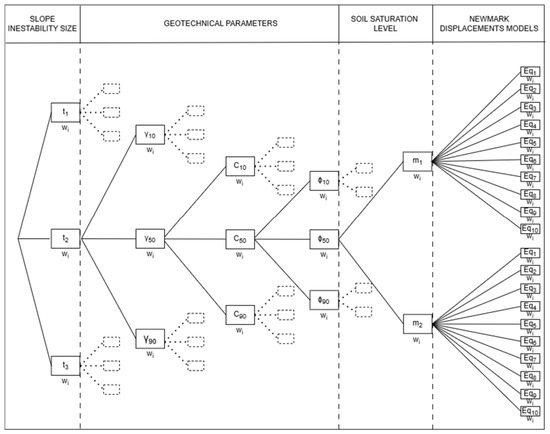
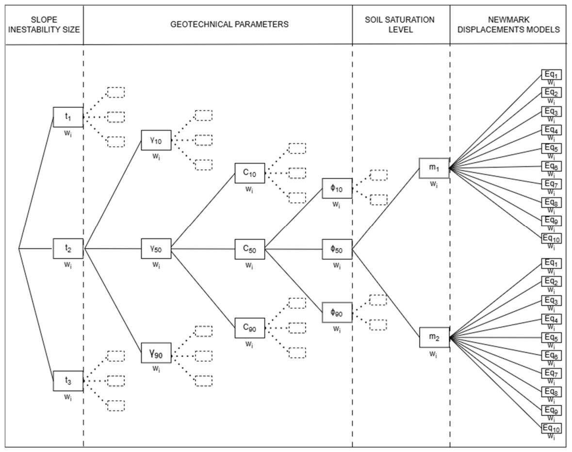
D_N computation by empirical equations cannot include the spatial variability of geotechnical parameters (unit weight, cohesion, and friction angle) within the same geological formation [28]. Similarly, it cannot account for the variability of failure depth and degree of saturation. To address such issues, a logic-tree methodology was proposed in previous works [22]. The logic tree is an analysis and planning technique that breaks down complex problems into simpler components, represented hierarchically in the form of a tree. It starts with a main objective, and branches into logically and sequentially related sub-objectives or actions. Each branch of the tree represents a possible alternative or solution, thereby facilitating understanding, analysis, and decision-making. The logic-tree structure used in this work is divided into six parts (Figure 1): failure depth, unit weight, cohesion, friction angle, degree of saturation, and D_N empirical equation.

Figure 1. Logic-tree structure used in the analysis. The weight used (w) is below the branch: t, failure surface depth (m); m, saturation degree; γ, unit weight; c’, effective cohesion; and ϕ’, friction angle for the 10th, 50th, and 90th percentiles; Eq: empirical equations for calculating Newmark displacement (Table 1).

The first part of the logic tree addresses the variability of the failure surface depth (t). Different values can be considered in the analysis, although typical values of failure depth range from 1 to 3 m [29,30].

The next three parts of the logic-tree structure are related to the geotechnical data: unit weight, cohesion, and friction angle of the geological material. To incorporate variability in each of these parameters, the values of the 10th, 50th, and 90th percentiles of the corresponding geotechnical property are considered. Selection of those percentiles follows a statistical adjustment of the variability of each geotechnical property to a triangular distribution [31].

The fifth part of the logic tree refers to the degree of saturation (m). Different degrees of saturation values can be considered, but normally, at least two situations should be considered: dry ground, representing surface materials during dry, warm periods without rain; and full saturation, to account for rainy days that can saturate the shallow ground.

The sixth part of the logic tree introduces the different D_N empirical equations used; in this work, D_N equations considered are the ones given in Table 1.

With the logic-tree approach, D_N is not reduced to a single value when characterizing the geotechnical properties of the slope, but rather incorporates the epistemic uncertainties associated with the geotechnical data, failure depth, and degree of saturation, by combining such factors in their branches. When the logic tree is applied to a territory, it yields a great number of maps, one for each combination of variables following branch after branch. For instance, if the number of failure depths is set to 3 and number of degrees of saturation is 2, the total number of susceptibility maps obtained using the logic-tree approach per D_N equation considered is 162 (three variables for failure depth, three for unit weight, three for cohesion, three for friction angle and two for degree of saturation). If 11 D_N equations are considered, 1782 susceptibility maps are generated.

Each branch of the logic tree can also be adjusted by adding weights. This leads to reflecting the geodynamic reality of a particular area more accurately. Weight values should be therefore based on an analysis of the co-seismic-induced landslides hazard in the area under study [22]. Different weights can be assigned to alternative values of the same parameter to reflect their relative plausibility. For instance, the 50th percentile of unit weight or friction angle are normally given higher weights because they represent the most typical conditions, whereas the 10th and 90th percentiles correspond to less frequent but still plausible extremes, and therefore lower weights are assigned. Similarly, Newmark equations with broader empirical support in similar geological and seismic settings may be weighted more highly than those with more limited applicability. These weights encode epistemic uncertainty and ensure that the final susceptibility map reflects both the central tendency and the plausible variability of the input parameters.

Once weights are known and applied, the logic-tree approach will produce susceptibility maps associated with a global weight value obtained as the product of the weights of each branch used to produce each map. This facilitates different scenarios to be analyzed, such as the one with the highest or lowest global weight, the ones that follow a given parameter, or even a weighted average scenario. Since weights are also applied to D_N equations, the resulting weighted susceptibility map also considers the suitability of each D_N equation for the area under study.

3. Design and Implementation of COSISA Software

3.1. Required Input Data

COSISA operates entirely with raster-based input layers, allowing each pixel to carry its own geotechnical, seismic, and morphometric values. As a result, the model naturally accommodates spatial variability across the study area, and no manual subdivision into zones is required. All susceptibility calculations are performed on a per-pixel basis, ensuring that local differences in material properties, slope conditions, or seismic intensity are fully represented in the final outputs.

Input data can be divided into three types: data introduced as georeferenced raster maps, D_N equations, and data given as a numerical value. Georeferenced raster datasets are provided in ArcGIS format: single-band floating-point raster datasets stored as ESRI Grid or within a File Geodatabase (GeoTIFF files can also be loaded after conversion to the ESRI Grid format). Raster inputs must share the same spatial resolution, spatial extent, and coordinate reference system to ensure consistency in calculations. These datasets comprise: the slope angle (in decimal degrees), the PGA (in g units), the I_A (in m/s), the 10th, 50th and 90th percentile of unit weight (3 maps, in kN/m³), the 10th, 50th and 90th percentile of cohesion (3 maps, in kN/m²), and the 10th, 50th and 90th percentile of the friction angle (3 maps, in decimal degrees). Equations for calculating D_N correspond to those 11 expressions shown in Table 1.

Numerical values include seismic moment (M_w) of the area under study, failure depth (t), degree of saturation (m), minimum slope angle to consider in calculations, and logic-tree weights. The user can define (see Section 3.4) from 1 to 4 failure depths (in m), as well as from 1 to 4 degrees of saturation values (in percentage, 0 meaning dry ground, 100 meaning full saturation). Minimum slope angle is defined to expedite the calculation process; this functions as a filter, so those points in the study area where slope angles are lower than the value introduced are removed from calculations as they are considered not susceptible. These pixels are assigned a NoData value in all susceptibility maps generated. The logic-tree weights (in parts per unit) are associated with each failure depth, each degree of saturation value defined, the 10th, 50th and 90th percentile of the unit weight, cohesion and friction angle (3 weights per geotechnical property), and each D_N equation selected.

3.2. Output Data

Output data consists of a series of georeferenced raster maps in ArcGIS format. For each combination provided by the logic tree, a susceptibility map with the corresponding D_N value calculated is obtained.

A weighted susceptibility map is also generated by combining all the output maps weighted by the global weight of each map (such global weight is obtained as the product of the weights of each branch used to produce this map). Before computing the final weighted susceptibility map, COSISA normalizes the global weights associated with each logic-tree branch. The global weight of each susceptibility map is first calculated as the product of the weights assigned to the selected branches. These global weights are then normalized (i.e., divided by the sum of all global weights) so that their sum equals 1.0, ensuring that the weighted average is consistent and that each scenario contributes proportionally to the final map. This normalization step guarantees that the weighted susceptibility map reflects the relative importance of all logic-tree combinations in a mathematically coherent manner.

During the weighted-map calculation, NoData pixels are ignored in the averaging process, and their NoData status is preserved in the final output. This ensures that areas with insufficient slope to generate co-seismic landslides remain consistently masked across all scenarios.

3.3. Program Structure

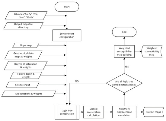
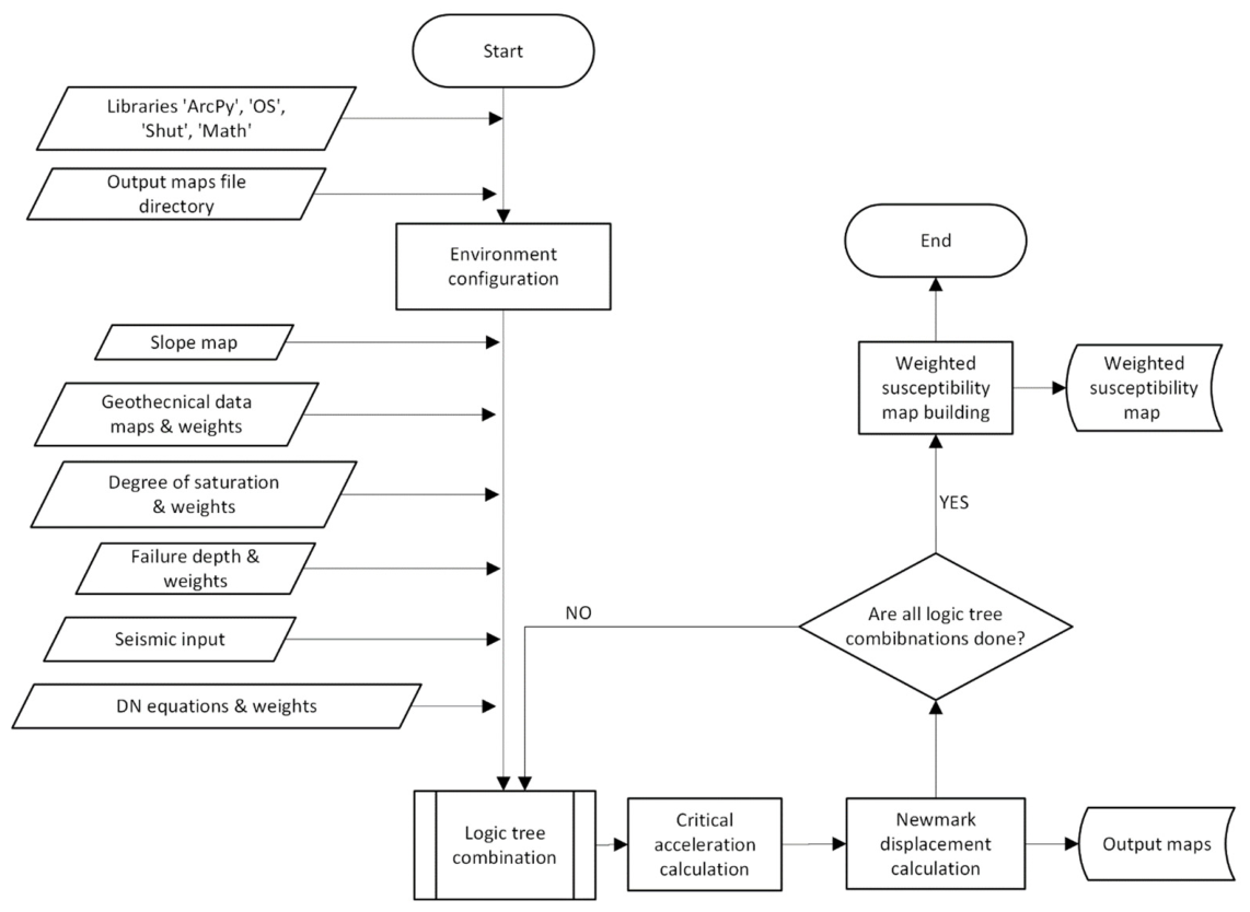
COSISA code is written in Python 2.7 to ensure full compatibility with ArcGIS 10.3, which relies on Python 2.7 as its native environment. The program is based on a graphical user interface (GUI) that utilizes the Tkinter and ttk libraries, making user interaction with input data easier. The flowchart in Figure 2 shows the main sequence of COSISA software. Such an algorithm runs in the background of the GUI, integrated as a sub-module of it, and is triggered when the user presses a calculation button (see Section 3.4). That button becomes active once all input data fields in the GUI are completed.

Figure 2. COSISA software flowchart with the main processes carried out by the program.

The first process entails environment configuration. Several Python libraries are imported: ‘ArcPy’, an ArcGIS library for geospatial calculations; the ‘OS’ and ‘Shutil’ libraries for file and directory management in the operating system; and the ‘Math’ library for handling advanced mathematical functions. Then, the output location and the output folder structure are defined, and geodatabase (gdb) directories are created to organize and store the output maps within the previously generated folder structure.

All the input data need to be loaded before going forward. This includes data not affected by the logic tree, i.e., slope angle map and seismic input data (PGA map, I_A map and M_w, the latter two if needed); and data concerned by the logic tree, i.e., the unit weight, cohesion and friction angle maps (3 maps for each variable, for the 10th, 50th and 90th percentiles, respectively), the degree of saturation values to consider, the failure values to consider, and the D_N equations selected (identified by an acronym of their authors as in Table 1). For those latter variables, the logic-tree weights associated with each one are also transferred to the algorithm.

The next process deals with the development of the logic tree. For each combination provided by the logic tree, the critical acceleration is calculated in ArcGIS for each point of the terrain, following Equation (1). From it, and with the seismic input data, each D_N equation selected to be considered is also computed in ArcGIS. The corresponding map is then outputted and stored as a geodatabase, named following the scheme DN_m_gamx_cy_fiz_t, where DN is the identification name of the Newmark displacement equation (e.g., JR07_1), m is the degree of saturation value, x, y, and z are the corresponding percentiles for unit weight (γ), cohesion (c), and friction angle (ϕ), respectively, and t is the failure depth value.

Once all the logic-tree combinations are done, the final process consists of combining all the maps produced according to their global weights to output a weighted map, also stored as a geodatabase and named as average.

3.4. Graphical User Interface

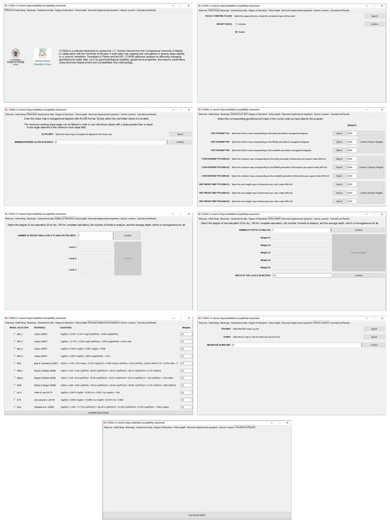
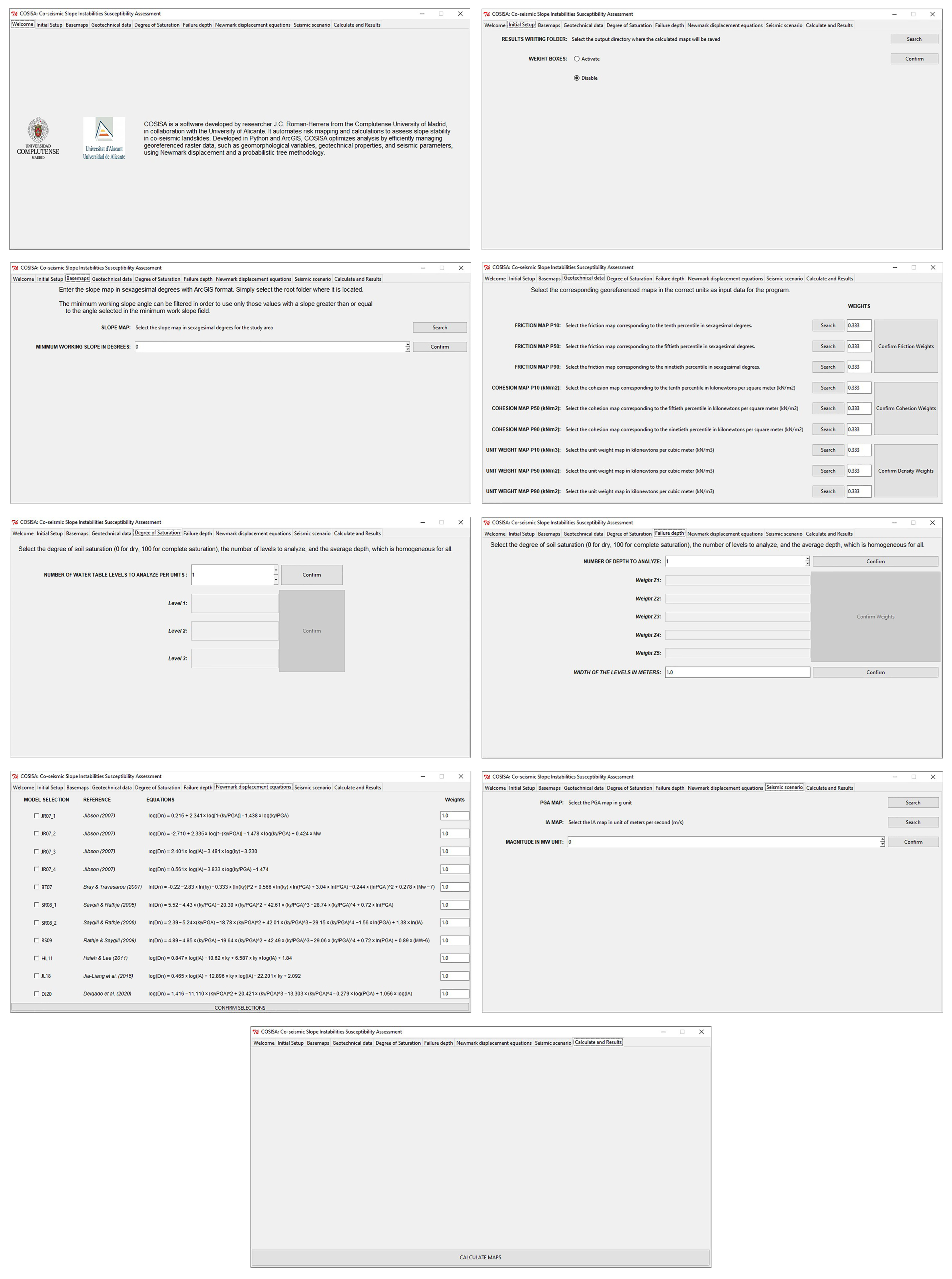
A GUI facilitates introduction of all input data, definition of logic-tree weights and running the program. The GUI is organized into 9 sequential tabs (Figure 3): “Welcome”, “Initial Setup”, “Base Maps”, “Geotechnical Data”, “Degree of Saturation”, “Failure Depth”, “Newmark Displacement Equations”, “Seismic Scenario” and “Calculate and Results”. Note that, by default, all logic-tree weights are equal to 1.0 in the GUI; not changing such value in any variable is equivalent to running the program without considering weights (since all weights have the same value).

Figure 3. Screen flow of the COSISA software for susceptibility evaluation.

The first tab of the GUI is the “Welcome” tab, which shows the COSISA logo and a welcome message. It also includes a brief description of the software.

The second tab is the “Initial Setup”. Here, one can select the working folder where all calculations generated by the program will be stored. Additionally, it includes a selector that allows users to decide whether the calculations will be performed with weights or not. To confirm this choice, it is necessary to click the “Confirm” button, as the decision will be final for that execution of the program.

The third tab is the “Base Maps” tab. Here, the user provides the georeferenced slope angle map, in decimal degrees and in ArcGIS format, by selecting the corresponding file in a file directory window. The user also has to define the minimum slope angle to consider (in decimal degrees, points with slope angles below it are assigned a NoData value and removed from calculations) after which they must confirm and save it by clicking the “Confirm” button.

The fourth tab corresponds to the “Geotechnical Data” tab. This is used to provide all the georeferenced geotechnical maps, in ArcGIS format, by selecting the corresponding files (a search button which opens a file directory). A total of 9 maps must be provided: the 10th, 50th, and 90th percentile of the unit weight (in kN/m³), the 10th, 50th, and 90th percentile of the cohesion (in kN/m²) and the 10th, 50th, and 90th percentile of the friction angle (in decimal degrees). Next to each search button, there is a space to enter the weight assigned to each map as a numerical value. The user must confirm and save the weight by clicking the “Confirm” buttons.

The fifth tab is the “Degree of Saturation” tab. Here, the user defines how many degrees of saturation values are to be considered. Once that number is specified, input boxes are activated to enter the different values considered (in percentage). Next to each degree of saturation, the corresponding weight can be entered as a numerical value. The user must confirm and save the weight by clicking the “Confirm” button.

The sixth tab is the “Failure Depth” tab. Like the previous tab, the user must define how many failure depth values are to be considered. Once specified that number, input boxes are activated to enter the different values considered (in m). Next to each depth, the corresponding weight can be entered as a numerical value. The user must confirm and save the weight by clicking the “Confirm” button.

The seventh tab corresponds to the “Newmark Displacement Equations” tab. Here, the user can select the D_N equations (Table 1) the study must consider by checking the corresponding checkboxes. Next to each checkbox, there is a space to enter the weight as a numerical value assigned to each D_N equation. Weights must be confirmed by clicking the “Confirm selections” button.

The eighth tab is the “Seismic Scenario” tab. This is used to provide the seismic input: (i) the PGA map (in g units) and (ii) the I_A map (in m/s), both in ArcGIS format and by selecting the corresponding files (search button); and (iii) the value of the moment magnitude M_w, entered as a numerical value. If no selected D_N equations require I_A and/or M_w, the corresponding input fields will be disabled.

The ninth and last tab is the “Calculate and Results” tab. The execution of the program will be initiated with the previously selected configurations by clicking the “Calculate maps” button. Upon completion of the calculation, a notification will appear on this screen indicating the end of the process.

The GUI of COSISA incorporates an internal validation system that ensures all required inputs are correctly provided before the computation begins. Each tab includes a confirmation step, and the “Calculate maps” button remains disabled until all mandatory fields are validated. This prevents the execution of the program with incomplete or unconfirmed inputs and ensures that the logic-tree configuration, geotechnical maps, and seismic parameters and weights are fully defined before processing. This built-in error-handling mechanism guarantees consistent and reproducible execution of the software.

4. Example of Application of COSISA Software

4.1. Case Study

The performance of COSISA software was performed in an area located at the province of Granada (southeastern Spain) where rock falls triggered during the 2021 Santa Fe seismic events were recorded. The province of Granada is the most seismically active region of Spain and is well-known for experiencing co-seismic landslides. Geologically, Granada is in the central part of the Betic Cordillera [32], in the intramountain Granada basin. At the northern and eastern edges of that basin, a series of normal faults are known to be active since the Pleistocene, having also identified active faults in the central sector of the basin [33,34]. Characterized by low-to-moderate seismic hazard, the basin has experienced several strong magnitudes and damaging earthquakes [35].

In a previous work, ref. [36] studied the susceptibility of two roads (A-92 highway and A-338 conventional road) of the Granada basin where co-seismic landslides were recorded during the Santa Fe seismic series. This was a series of very low to low-magnitude earthquakes that occurred from January to November 2021 [37]. Depths of these seismic events ranged from 3 to 5 km, reaching a magnitude (M_w) of 4.4. The authors used the methodology based on the Newmark displacement and a logic-tree approach for developing co-seismic landslide susceptibility maps. This work verified and validated the appropriateness of the weights proposed by [22] for landslides triggered by the 2011 Lorca earthquake (M_w 5.1).

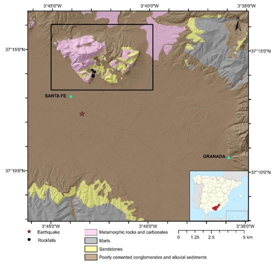
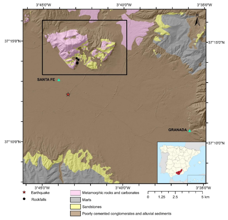
Since the study area of the present work is located in the Granada basin, the weights fixed can be applied here. Figure 4 shows the area under study, where outcropping lithologies can be broadly divided into four main geotechnical groups (Table 2). The basement materials consist of Mesozoic sedimentary rocks from the External Zones of the mountain range in the northern and western boundaries, and Paleozoic to Triassic metamorphic rocks from the Internal Zones in the southern and eastern boundaries. The basin fill comprises sedimentary rocks from the Burdigalian (Miocene) to the Quaternary [38]. The sedimentary fill is primarily composed of conglomerates, sandstones, marls, and limestones during the Miocene. From the Pliocene and Pleistocene, thick deposits of conglomerates and sandstones were formed; there are alluvial sediments related to the present-day rivers.

Figure 4. Geological map of the Granada basin (SE Spain). In the lower right corner, there is a map of the Iberian Peninsula, with the province of Granada highlighted in red. The case study area is indicated by a black rectangle. The red star shows the epicenter of the mainshock of the 2021 Santa Fe seismic series and black circles the location of rock falls triggered by it.

Table 2. Geotechnical properties of materials found in the study area [22]: γ, unit weight (kN/m³); c’, effective cohesion (kPa); and ϕ’, effective friction angle (°) for the 10th, 50th, and 90th percentiles (p10, p50, p90).

	Conglomerates			Calcareous Sandstones			Metamorphic Rocks and Carbonates
	γ	c’	ϕ’	γ	c’	ϕ’	γ	c’	ϕ’
Low (p10)	15.40	4.91	17.00	15.12	4.02	19.00	22.66	0.00	30.00
Best (p50)	18.13	33.35	26.00	16.19	17.17	24.00	26.88	13.73	36.00
High (p90)	24.42	90.12	35.00	16.86	51.89	30.00	27.96	247.02	49.00

4.2. Input Data

The study was done using a slope angle map which was computed from a digital elevation model at a pixel size of 5 × 5 m obtained at the Spanish Geographic Institute [39]. The geotechnical maps (10th, 50th, and 90th percentile of unit weight, cohesion, and friction angle) were prepared from polygon vector maps carried out by the Spanish Geological Survey [40] and by considering the values showed in Table 2 for the geotechnical properties. The geological vector layers were converted to a raster with the same pixel size as the slope map (5 × 5 m), producing piecewise-constant percentile maps per geological formation. This approach preserves the geological layout, while avoiding artificial smoothing of interpolation techniques (e.g., kriging or inverse distance weighting) across lithological boundaries.

Three values of failure depth were considered: 1, 2, and 3 m. These values follow the work conducted previously [22] and considers that failure depths of 2 and 3 m are common values for landslides induced by low-to-moderate magnitude earthquakes in Spain [29,30]. As a degree of saturation, two values were considered: 0 (dry conditions), and 100 (full saturation).

From the eleven D_N equations provided by COSISA software (Table 1), six were considered for calculation (JR07_3, JR07_4, SR08_2, RS09, HL11, and DJ20). These equations were chosen because they depend exclusively on PGA, I_A, and/or M_w, which were the seismic parameters available for the 2021 Santa Fe seismic series.

The dynamic conditions of the study area were considered by PGA and I_A raster maps, considering a 475-year return period probabilistic seismic scenario. PGA values in the study area vary from 0.23 g (northwest sector) to 0.32 g (southeast sector), reflecting the influence of site conditions and source-to-site distance on the seismic input. Average values for PGA and I_A were 0.28 g and 0.33 m/s, respectively. M_w was set to 5.1 [22].

Weights (Table 3) were obtained for the 2011 Lorca earthquake in equivalent geological materials and seismotectonic contexts to those of the studied area [22].

Table 3. Logic-tree weights for the case study analyzed.

Variable		Weight
Failure depth	1.0 m	0.528
	2.0 m	0.405
	3.0 m	0.067
Degree of saturation	0.0	0.500
	1.0	0.500
Unit weight	10th percentile	0.333
	50th percentile	0.333
	90th percentile	0.333
Cohesion	10th percentile	0.533
	50th percentile	0.281
	90th percentile	0.186
Friction angle	10th percentile	0.269
	50th percentile	0.384
	90th percentile	0.347
DN equation	JR07_3	0.175
	JR07_4	0.172
	SR08_2	0.155
	RS09	0.172
	HL11	0.162
	DJ20	0.163

4.3. Output Maps

The use of 10th, 50th, and 90th percentile geotechnical maps introduces a wide range of possible Newmark displacement values. This variability is intentionally propagated through the logic-tree structure, where each percentile map generates a separate susceptibility scenario. As a result, the output distribution reflects the full range of plausible geotechnical conditions. Although individual scenarios may differ substantially, the weighted susceptibility map integrates all branches according to their assigned weights, preventing contradictory interpretations and providing a single, uncertainty-aware representation of co-seismic landslide susceptibility. This approach ensures that the statistical dispersion of the outputs is explicitly considered rather than generalized or overlooked.

Having applied the COSISA software, 972 seismic landslide susceptibility maps in terms of Newmark displacement were obtained. The total computation time for the case study was approximately 16 min. This value corresponds to processing a raster dataset of 5 × 5 m spatial resolution, comprising approximately 42.26 × 10⁶ pixels (exact number depending on the study area extent). Calculations were performed on a computer equipped with an Intel Core i5 (x64) processor, 8 GB RAM, NVIDIA GeForce GTX 1060 GPU and running ArcGIS with Python 2.7. Some of the resulting maps are presented as examples to show COSISA software’s potential use and application.

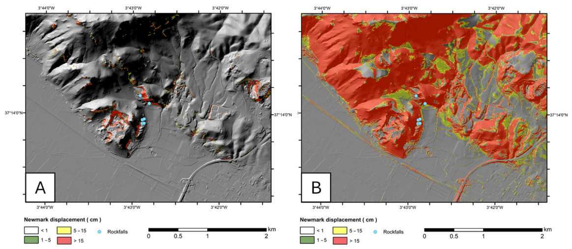
First, the susceptibility maps corresponding to the best- and worst-case models can be identified. The best case (Figure 5A) corresponds to the parameter combination with the highest success rate [22], comprising the following set of parameters: depth of failure surface of 2 m, percentile 10th of unit weight, percentile 10th of cohesion, percentile 90th of friction angle, degree of saturation of 0 (dry conditions), and Newmark displacement model SR08_1 by [5]. The worst scenario (Figure 5B) corresponds to the most unfavorable combination of parameters considering the weights defined: depth of failure surface of 3 m, percentile 90th of unit weight, percentile 10th of cohesion, percentile 10th of friction angle, degree of saturation of 100 (full saturation), and Newmark displacement model HL11 by [6].

Figure 5. Susceptibility maps in terms of Newmark displacements obtained with the logic-tree methodology for case study area. (A) Best case with the highest success rate considering a probabilistic seismic scenario for a return period of 475 years. (B) Worst case (conservative) considering a probabilistic seismic scenario for a return period of 475 years. Rock falls triggered by the 2021 Santa Fe seismic series are depicted as light blue circles.

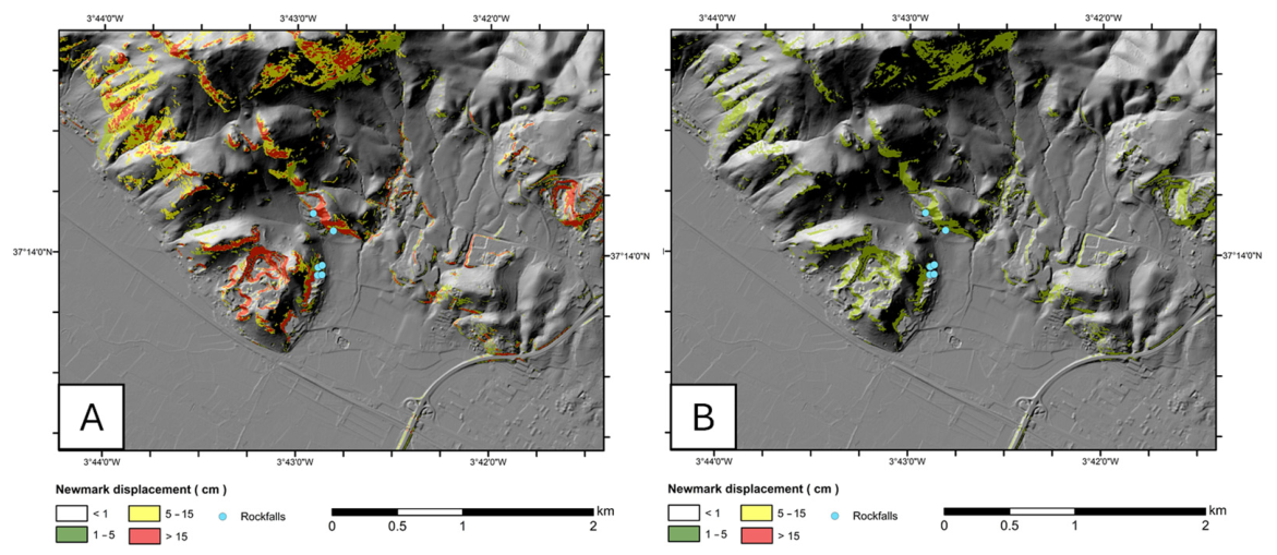
Considering all the individual weights of each susceptibility map, a final weighted map was obtained, which considers all the variability of the parameters and D_N equations. An advantage of using the COSISA software is that it allows the obtaining of weighted maps for different probabilistic and deterministic input seismic scenarios (Figure 6).

Figure 6. Weighted susceptibility maps in terms of Newmark displacements obtained with the logic-tree methodology for case study area. (A) Deterministic seismic scenario for the 2021 Santa Fe seismic series. (B) Probabilistic seismic scenario for a return period of 475 years. Rock falls triggered by the 2021 Santa Fe seismic series are depicted as light blue circles.

The accuracy of the susceptibility maps generated by COSISA was evaluated by comparing the results with the inventory of rock falls triggered during the 2021 Santa Fe seismic series. The locations of documented co-seismic failures (Figure 4) coincide with areas classified as moderate-to-high susceptibility in the COSISA output, particularly in the weighted scenario (Figure 5 and Figure 6). This agreement confirms that the methodology and the previously calibrated logic-tree weights provide reliable susceptibility estimates for the Granada Basin.

5. Discussion

The COSISA software provides several advantages for co-seismic landslide susceptibility assessment. First, it automates a traditionally time-consuming workflow by integrating geotechnical, geomorphological, and seismic data within a single Python–GIS environment. This significantly reduces the manual effort required to generate multiple susceptibility scenarios. In addition, the implementation of a logic-tree framework allows COSISA to incorporate epistemic uncertainty associated with geotechnical parameters, failure depth, degree of saturation, and the selection of Newmark displacement equations. This approach enables the generation of many susceptibility maps and supports the identification of best- and worst-case scenarios, as well as weighted susceptibility outcomes.

Despite these strengths, COSISA also presents some limitations. The software relies on the availability and quality of geotechnical and seismic input data, which may vary across regions.

A limitation of the current COSISA version is that failure depth is treated as a uniform value within each branch of the logic tree. This approach follows previous studies and reflects the epistemic uncertainty associated with shallow failure depths, which are often poorly constrained at regional scales. However, it does not capture the spatial variability of failure depth across the terrain. In the absence of detailed subsurface or geotechnical profiling, COSISA allows users to explore several possible failure depths (e.g., 1–3 m) through the logic-tree structure, but these values are applied uniformly to all pixels within each scenario. Future developments could incorporate spatially variable failure depth maps derived from geomorphological indicators, geophysical surveys, or machine-learning-based estimations to better represent local variability.

Additionally, the current version is implemented in Python 2.7 and depends on ArcGIS libraries, which may limit portability and long-term maintenance. The empirical Newmark displacement equations used also have inherent constraints, as they were developed for specific earthquake datasets and may not fully capture local seismic characteristics in all regions.

The validation of COSISA results was performed by comparing the susceptibility maps with the inventory of rockfalls triggered during the 2021 Santa Fe seismic sequence. Although quantitative performance metrics such as AUC or success rate are commonly used in statistical susceptibility models, their application here is limited by the small number of documented failures and their spatial clustering. Under these conditions, such metrics would not yield statistically meaningful results. For this reason, validation was based on spatial agreement between observed failures and areas classified as moderate-to-high susceptibility, following the approach adopted in previous studies in Betic Cordillera. This limitation is inherent to regions where co-seismic landslide inventories are scarce, and it highlights the need for more comprehensive post-earthquake mapping to enable robust quantitative validation in future work.

There is a possibility for improvement in future versions of COSISA. Potential enhancements include migrating the code to Python 3.x, incorporating open-source GIS alternatives to increase accessibility, integrating additional empirical or numerical models for displacement estimation, and developing tools for automatic calibration using landslide inventories. Expanding the software to include probabilistic seismic hazard inputs or dynamic ground-motion simulations could further improve its applicability in complex tectonic settings.

6. Conclusions

A new software (COSISA) was developed for assessing co-seismic slope instabilities susceptibility based on the Newmark displacement and a logic-tree procedure from geomorphology, geotechnical properties, and seismic parameters.

The COSISA software significantly reduces the workload and time needed for the susceptibility map generation process. It also leads to a fast definition of the best- and worst-case models, i.e., the one with a parameter combination with the highest success rate and the one with the most unfavorable combination of parameters, respectively.

Producing many susceptibility maps, which incorporate various combinations of input parameters, allows for the assessment of different scenarios (deterministic and/or probabilistic). This facilitates the evaluation of how each geotechnical parameter influences co-seismic landslide susceptibility and helps in analyzing the effectiveness of various Newmark displacement equations.

Application of the COSISA software is shown by studying an area of the Granada basin (southeastern Spain), where some of the rock falls triggered during the 2021 Santa Fe seismic events were recorded. The susceptibility maps obtained correspond to the best- and worst-case models, and the weighted susceptibility maps considering different input seismic scenarios (determinist and probabilistic). The integration of COSISA into the co-seismic landslide susceptibility analysis workflow marks a transformative shift toward efficiency and automation. With this code, we successfully generated multiple susceptibility maps in a single operation, significantly reducing time and effort. This automated approach produced a comprehensive set of results; all achieved with remarkable speed. Conversely, when conducting parallel analyses using a traditional, step-by-step process, identical results were achieved; however, the process was notably slower, highlighting the substantial time-saving benefits offered by COSISA’s automation. This not only underscores COSISA’s effectiveness in data processing, but emphasizes its potential to also streamline workflows, providing users with a fast, intuitive alternative to traditional methods.

COSISA software can also be utilized to determine the weights for an area where these weights are not known, but where there is an inventory of earthquake-triggered landslides. In such cases, a calibration process involving multiple runs can be performed, comparing the predictive success of the generated maps with the empirical recorded data. Once this calibration process is complete, the obtained weights can be applied to other study areas in the vicinity. The software can then be used to predict co-seismic landslide susceptibility in the new area, by considering different seismic scenarios.

In conclusion, the use and implementation of COSISA software can aid in territorial planning and hazard management strategies, thereby reducing the damage from future co-seismic landslides.

References

- Marano, K.D.; Wald, D.J.; Allen, T.I. Global earthquake casualties due to secondary effects: A quantitative analysis for improving rapid loss analyses. Nat. Hazards 2010, 52, 319–328. [Google Scholar] [CrossRef] [Scilit]
- Daniell, J.E.; Schaefer, A.M.; Wenze, F. Losses Associated with Secondary Effects in Earthquakes. Front. Built Environ. 2017, 3, 30. [Google Scholar] [CrossRef] [Scilit]
- Jibson, R.W. Predicting earthquake-induce landslide displacements using Newmark’s sliding analysis. Transp. Res. Rec. 1993, 1411, 9–17. [Google Scholar]
- Jibson, R.W. Regression models for estimating coseismic landslide displacement. Eng. Geol. 2007, 91, 209–218. [Google Scholar] [CrossRef] [Scilit]
- Saygili, G.; Rathje, E.M. Empirical predictive models for earthquake-induced sliding displacements of slopes. J. Geotech. Geoenviron. Eng. 2008, 134, 790–803. [Google Scholar] [CrossRef] [Scilit]
- Hsieh, S.Y.; Lee, C.T. Empirical estimation of the Newmark displacement from the Arias intensity and critical acceleration. Eng. Geol. 2011, 122, 34–42. [Google Scholar] [CrossRef] [Scilit]
- Delgado, J.; Rosa, J.; Peláez, J.A.; Rodríguez-Peces, M.J.; Garrido, J.; Tsige, M. On the applicability of available regression models for estimating Newmark displacements for low to moderate magnitude earthquakes. The case of the Betic Cordillera (S Spain). Eng. Geol. 2020, 274, 105710. [Google Scholar] [CrossRef] [Scilit]
- Chousianitis, K.; del Gaudio, V.; Kalogeras, I.; Ganas, A. Predictive model of Arias intensity and Newmark displacement for regional scale evaluation of earthquake-induced landslide hazard in Greece. Soil Dyn. Earthq. Eng. 2014, 65, 11–29. [Google Scholar] [CrossRef] [Scilit]
- Jessee, M.A.N.; Hamburger, M.W.; Allstadt, K.; Wald, D.J.; Robeson, S.M.; Tanyas, H.; Hearne, M.; Thompson, E.M. A global empirical model for near-mapped-time assessment of seismically induced landslides. J. Geophys. Res. Earth Surf. 2018, 123, 1835–1859. [Google Scholar] [CrossRef] [Scilit]
- Román-Herrera, J.C.; Rodríguez-Peces, M.J.; Garzón-Roca, J. Comparison between Machine Learning and Physical Models Applied to the Evaluation of Co-Seismic Landslide Hazard. App. Sci. 2023, 13, 8285. [Google Scholar] [CrossRef] [Scilit]
- Rathje, E.M.; Antonakos, G. A unified model for predicting earthquake-induced sliding displacements of rigid and flexible slopes. Eng. Geol. 2011, 122, 51–60. [Google Scholar] [CrossRef] [Scilit]
- Gong, W.; Zekkos, D.; Clark, M. The influence of seismic displacement models on spatial prediction of regional earthquake-induced landslides. Eng. Geol. 2023, 325, 107288. [Google Scholar] [CrossRef] [Scilit]
- Rathje, E.M.; Bray, J.D. An examination of simplified earthquake-induced displacement procedures for earth structures. Can. Geotech. J. 1999, 36, 72–87. [Google Scholar] [CrossRef]
- Rathje, E.M.; Bray, J.D. Nonlinear coupled Seismic Sliding Analysis of Earth Structures. J. Geotech. Geoenviron. Eng. 2000, 126, 1002–1014. [Google Scholar] [CrossRef] [Scilit]
- Guzzetti, F.; Reichenbach, P.; Cardinali, M.; Galli, M.; Ardizzone, F. Probabilistic Landslide Hazard Assessment at the Basin Scale. Geomorphology 2005, 72, 272–299. [Google Scholar] [CrossRef] [Scilit]
- Furlani, S.; Ninfo, A. Is the Present the Key to the Future? Earth-Sci. Rev. 2005, 142, 38–46. [Google Scholar] [CrossRef] [Scilit]
- Mercurio, C.; Calderón-Cucunuba, L.P.; Argueta-Platero, A.A.; Azzara, G.; Cappadonia, C.; Martinello, C.; Rotigliano, E.; Conoscenti, C. Predicting Earthquake-Induced Landslides by Using a Stochastic Modeling Approach: A Case Study of the 2001 El Salvador Coseismic Landslides. ISPRS Int. J. Geo-Inf. 2023, 12, 178. [Google Scholar] [CrossRef] [Scilit]
- Chuang, R.Y.; Wu, B.S.; Liu, H.C.; Huang, H.H.; Lu, C.H. Development of a statistics-based nowcasting model for earthquake-triggered landslides in Taiwan. Eng. Geol. 2021, 89, 106177. [Google Scholar] [CrossRef] [Scilit]
- Kavianpour, P.; Kavianpour, M.; Jahani, E.; Ramezani, A. A CNN-BiLSTM model with attention mechanism for earthquake prediction. J. Supercomput. 2023, 79, 19194–19226. [Google Scholar] [CrossRef] [Scilit]
- Montoya-Araque, E.A.; Montoya-Noguera, S.; Lopez-Caballero, F. An open-source application software for spatial prediction of permanent displacements in earthquake-induced landslides by the Newmark sliding block method: PyNewmarkDisp. Environ. Model. Softw. 2024, 173, 105942. [Google Scholar] [CrossRef] [Scilit]
- Ji, J.; Cui, H.; Zhang, T.; Song, J.; Gao, Y. A GIS-based tool for probabilistic physical modelling and prediction of landslides: GIS-FORM landslide susceptibility analysis in seismic areas. Landslides 2022, 19, 2213–2231. [Google Scholar] [CrossRef] [Scilit]
- Rodríguez-Peces, M.J.; Román-Herrera, J.C.; Peláez, J.A.; Delgado, J.; Tsige, M.; Missori, C.; Martino, S.; Garrido, J. Obtaining suitable logic-tree weights for probabilistic earthquake-induced landslide hazard analyses. Eng. Geol. 2020, 275, 105743. [Google Scholar] [CrossRef] [Scilit]
- Newmark, N.M. Effects of earthquakes on dams and embankments. Géotechnique 1965, 15, 139–160. [Google Scholar] [CrossRef] [Scilit]
- Jibson, R.W.; Michael, J.A. Maps Showing Seismic Landslide Hazards in Anchorage, Alaska (Version 1.0); U.S. Geological Survey Scientific Investigations Map 3077, Report: Iv; U.S. Geological Survey: Reston, VA, USA, 2009; 11p. [CrossRef] [Scilit]
- Bray, J.D.; Travasarou, T. Simplified procedure for estimating earthquake-induced deviatoric slope displacements. J. Geotech. Geoenviron. Eng. 2007, 133, 381–392. [Google Scholar] [CrossRef] [Scilit]
- Rathje, E.M.; Saygili, G. Probabilistic assessment of earthquake-induced sliding displacements of natural slopes. Bull. N. Z. Soc. Earthq. Eng. 2009, 42, 18–27. [Google Scholar] [CrossRef] [Scilit]
- Jia-Liang, J.; Yin, W.; Dan, G.; Ren-Mao, Y.; Xiao-Yan, Y. New evaluation models of Newmark displacement for southwest China. Bull. Seismol. Soc. Am. 2018, 108, 2221–2236. [Google Scholar] [CrossRef] [Scilit]
- Dreyfus, D.; Rathje, E.M.; Jibson, R.W. The influence of different simplified sliding block models and input parameters on regional predictions of seismic landslides triggered by the Northridge earthquake. Eng. Geol. 2013, 163, 41–54. [Google Scholar] [CrossRef] [Scilit]
- Alfaro, P.; Delgado, J.; García-Tortosa, F.J.; Lenti, L.; López, J.A.; López-Casado, C.; Martino, S. Widespread landslides induced by the Mw 5.1 earthquake of 11 May 2011 in Lorca. SE Spain. Eng. Geol. 2012, 137–138, 40–52. [Google Scholar] [CrossRef] [Scilit]
- Rodríguez-Peces, M.J.; García-Mayordomo, J.; Martínez-Díaz, J.J. Slope instabilities triggered by the 11th May 2011 Lorca earthquake (Murcia, Spain): Comparison to previous hazard assessments and proposition of a new hazard map and probability of failure equation. Bull. Earthq. Eng. 2013, 12, 1961–1976. [Google Scholar] [CrossRef] [Scilit]
- Keefer, D.L.; Bodily, S.E. Three-point approximations for continuous random variables. Manag. Sci. 1983, 29, 595–609. [Google Scholar] [CrossRef] [Scilit]
- Azañón, J.M.; Galindo-Zaldívar, J.; García-Dueñas, V.; Jabaloy, A. Alpine tectonics II: Betic Cordillera and Balearic Islands. In The Geology of Spain; Gibbons, W., Moreno, T., Eds.; Geological Society of London: London, UK, 2002. [Google Scholar] [CrossRef] [Scilit]
- de Galdeano, C.S.; Peláez, J.A.; López-Casado, C. Seismic potential of the main active faults in the Granada Basin (Southern Spain). Pure Appl. Geophys. 2003, 160, 1537–1556. [Google Scholar] [CrossRef] [Scilit]
- de Galdeano, C.S.; García-Tortosa, F.J.; Peláez, J.A.; Alfaro, P.; Azañón, J.M.; Galindo-Zaldívar, J. Main active faults in the Granada and Guadix-Baza Basins (Betic Cordillera). J. Iber. Geol. 2012, 38, 209–223. [Google Scholar] [CrossRef] [Scilit]
- Madarieta-Txurruka, A.; Galindo-Zaldívar, J.; González-Castillo, L.; Peláez, J.A.; Ruiz-Armenteros, A.M.; Henares, J.; Garrido-Carretero, M.S.; Avilés, M.; Gil, A.J. High- and low-angle normal fault activity in a collisional orogen: The northeastern Granada Basin (Betic Cordillera). Tectonics 2021, 40, e2021TC006715. [Google Scholar] [CrossRef] [Scilit]
- Román-Herrera, J.C.; Delgado, J.; Rodríguez-Peces, M.J.; Peláez, J.A.; Garrido, J. Evaluation of road network slopes susceptibility to seismically-induced landslides in the Granada Basin (S Spain). Front. Earth Sci. 2023, 11, 2296–6463. [Google Scholar] [CrossRef] [Scilit]
- Lozano, L.; Cantavella, J.V.; Gaite, B.; Ruiz-Barajas, S.; Antón, R.; Barco, J. Seismic analysis of the 2020–2021 Santa Fe seismic sequence in the Granada Basin, Spain: Relocations and focal mechanisms. Seismol. Soc. Am. 2022, 93, 3246–3265. [Google Scholar] [CrossRef] [Scilit]
- Braga, J.C.; Martin, J.M.; Alcala, B. Coral reefs in coarse-terrigenous sedimentary environments (Upper Tortonian, Granada Basin, southern Spain). Sediment. Geol. 1990, 66, 135–150. [Google Scholar] [CrossRef] [Scilit]
- Instituto Geográfico Nacional (IGN). Lorca 953-III (49–76). In Mapa Topográfico Nacional 1:25.000; Instituto Geográfico Nacional (IGN): Madrid, Spain, 2017. [Google Scholar]
- Lupiani, E.; Soria, J. Mapa Geológico de España E. 1:50.000. Hoja 1009 (Granada); MAGNA 50; Instituto Geológico y Minero de España: Madrid, Spain, 1985. [Google Scholar]
Disclaimer/Publisher’s Note: The statements, opinions and data contained in all publications are solely those of the individual author(s) and contributor(s) and not of MDPI and/or the editor(s). MDPI and/or the editor(s) disclaim responsibility for any injury to people or property resulting from any ideas, methods, instructions or products referred to in the content. |
© 2026 by the authors. Licensee MDPI, Basel, Switzerland. This article is an open access article distributed under the terms and conditions of the Creative Commons Attribution (CC BY) license.