


Abstract
Reliable subsurface temperature estimates are crucial for most geoenergy projects, as they directly influence the properties of both rocks and fluids. They are particularly important in geothermal energy exploration, where errors in estimating the static formation temperature (SFT) can lead to significant misinterpretations, potentially resulting in incorrect classification of the geothermal resource. Various corrections are applied to bottom-hole temperatures (BHTs), with the Horner correction being the most widely used. In addition, empirical methods have been developed to improve accuracy at the local scale. In this study, maximum temperature values (Tmax) reported for deep exploration wells in the Sava and Drava Basins were compared to both Horner-corrected temperatures (HPCTs) and those recorded during drill-stem tests (TDST). In both basins, Tmax values frequently significantly diverge from HPCT measurements, emphasizing the limited reliability of Tmax for estimating subsurface temperatures. In the Sava Basin, 61% of wells show Tmax-HPCT differences greater than 10 °C, and in seven wells the discrepancy exceeds 20 °C. Similarly, in the Drava Basin, nearly half of the wells exhibit differences greater than 10 °C, with five wells showing deviations above 20 °C. In most cases, the reported Tmax values do not represent true maxima, so the linear regression was performed between Tmax and temperatures obtained from DST measurements, providing a basis for refining subsurface temperature estimates.
1. Introduction
Having a reliable estimate of the subsurface temperature is a requirement in most geoenergy projects [1,2]. However, the path to obtaining such reliable estimates is neither simple nor straightforward, with many possible pitfalls. So, estimating temperatures in the subsurface has been a longstanding challenge for researchers aiming to better understand the subsurface thermal regime [3,4,5].
Although subsurface temperature can be estimated from maximum-reading thermometers used during wireline logging or from continuous temperature logs [6], the reliability of their interpretation has improved surprisingly little. In contrast, logging techniques and their interpretation have advanced markedly. Modern workflows can now employ sophisticated machine learning frameworks capable of jointly predicting complex petrophysical properties and formation layering [7]. On the other hand, most widely used basic temperature measurements, bottom-hole temperatures (BHTs), typically derived from a single maximum-thermometer reading taken at the borehole bottom shortly after circulation stops, remain burdened by substantial uncertainty due to pronounced thermal nonequilibrium, e.g., as shown in [5,6]. Temperature logs, which are recorded along a substantial interval of the well and often continuously from the surface to total depth, can offer a more accurate view of the temperature distribution, especially when taken some time after mud circulation has ceased. The quality of continuous temperature logs varies due to differences in tool resolution and the length of shut-in periods before logging. Only when multiple temperature logs are recorded at different shut-in times can the progression toward thermal equilibrium be analyzed [8]. However, neither of these methods provides information on real temperatures in the subsurface (usually referred to as the static formation temperature, SFT). Förster (2001) [9] found that the large standard deviation of corrected BHT measurements, around ±8 °C, implies that even corrected BHT values may only approximate the true formation temperature within about ±16 °C. Moreover, this approximation systematically tends toward underestimation, with 74% of corrected BHTs falling below the actual formation temperature [9]. To accurately measure the true formation temperature after the cessation of drilling mud circulation, a thermal equilibrium must be established. This requires the dissipation of the cooling effect induced by mud circulation, allowing both the wellbore fluids and the thermally disturbed near-wellbore formation to re-equilibrate with the undisturbed static formation temperature [9]. To have more reliable data, temperature corrections are applied. However, they require multiple BHT measurements performed at the same depth at several time points after the stop of mud circulation.
Temperature measurements taken during Drill-Stem Testing (DST) are considered the most reliable formation temperature measurements in deep wells [10]. DST measurements yield an approximate SFT as long as the fluid is unaffected by thermal disturbances surrounding the well [11,12]. In that respect, some authors caution about the reliability of DST temperature readings in relation to the volume of produced formation fluids. The volume of extracted fluid should reach a certain threshold (>100 barrels) to allow the temperature to equilibrate with the formation temperature [12].
To address the issue of errors in BHT measurements, academic and industrial communities have developed various correction methods, among which the Horner correction method [13] is the most commonly used, in addition to corrections based on the spherical heat flow model [14] and statistically based empirical methods [3,15]. However, each of these methods has its own assumptions and applicable conditions: the Horner method relies on the simplification of the radial heat conduction model, the spherical model assumes spherical heat flow at the bottom of the well, and statistical methods require local data for calibration. More importantly, different methods may yield different correction results for the same well (with differences exceeding 10 °C in some cases [16]), introducing additional uncertainty into temperature estimation. Consequently, selecting an appropriate correction method for a given region, or establishing a localized empirical correction, has become an important challenge in geothermal exploration.
2. Temperature Corrections
This section will provide a systematic review of existing correction methods, laying the theoretical foundation for the methodological design of this study.
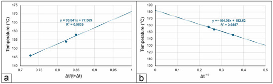
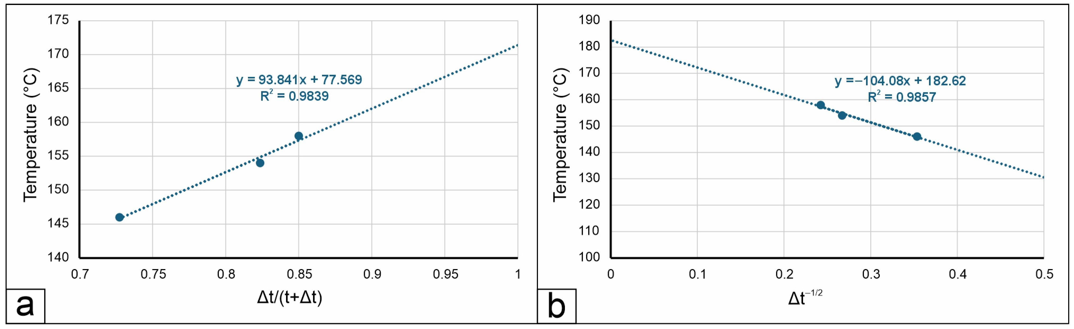
As already mentioned, temperature corrections can be applied if data from multiple temperature measurements taken at different time intervals at the same depth are available. The most widely used correction is Horner’s correction, which assumes radial thermal flow from the formation into the well. It is actually based on the Horner [13] equation for the assessment of formation pressure build-up and represents a simplification of a mathematical model developed by Bullard [5]. Measured temperature values (BHTs) are plotted on the ordinate in a linear scale, while the ratio Δt/(tc + Δt) for each corresponding temperature measurement is plotted on the abscissa in a logarithmic scale. Here, Δt represents the time elapsed since the cessation of mud circulation (also sometimes referred to as thermal relaxation time), expressed in hours, and tc is the duration of the mud circulation, also in hours. This approach yields a series of points (usually three), through which a line is drawn. The corrected temperature value (Tcorr) corresponds to the y-axis intercept of this line at the point where Δt/(tc + Δt) equals one (see Figure 1a), i.e., the point where the thermal equilibrium at infinite time is assumed.
Figure 1.
(a) An example of Horner plot correction—the static temperature is read at the point where the ordinate (Δt/(t + Δt)) equals 1, i.e., where an infinite time is assumed to have passed since mud circulation ceased; (b) an example of correction proposed by [14]—the static temperature is read at the point where the abscissa 1/√Δt equals 0, i.e., another approximation of infinite time passed since cessation of mud circulation.
The main challenge in determining the static temperature using Horner’s correction is the lack of data. Temperature measurements taken at precise intervals following the cessation of mud circulation have only been systematically recorded in well logging reports in exploration wells of the Croatian part of the Pannonian Basin from the 1980s onward, resulting in a limited dataset. Moreover, even in cases where complete temperature measurements were available, the record of the mud circulation duration was often missing. It should be noted that after [16], models that assume that the mud circulation acts as an instantaneous line temperature sink and neglect the well diameter are only valid for condition r2/4 κr Δt < 1, where r represents the well diameter (m), κr represents rock thermal diffusivity (m2/h) and Δt is the time elapsed since the cessation of mud circulation (h).
Another approach was described by [14] on the example of an exploration geothermal well in the Mexican Volcanic Belt. It is based on the spherical–radial heat flow at the bottom of the well. Over extended time intervals, this approach suggests a linear relationship when plotting registered BHT against 1/√Δt, where the axes’ intercept represents the equilibrium temperature. For presented case, this model resulted in somewhat higher corrected temperatures compared to Horner’s plot (Figure 1a,b).
Waples and Ramly [15] introduced a statistical correction factor for the correction of well-log temperatures, based on the time since the end of mud circulation and depth of the temperature measurement. In the presented case, DST temperatures from 40 wells in the Malay basin as reference temperatures for these corrections were used.
Aabø and Hermanrud [10] proposed an improved empirical model based on data from eight oil and gas fields on the Norwegian continental shelf. The model, validated using drill-stem test (DST) temperature data, provided more accurate static temperature estimates from single BHT measurements. However, prediction errors of up to 10 °C were found between fields and ref. [10] attributed them to differences in operational practices, especially in mud circulation practiced on different oil rigs in regard to varying mud pump rates and multiple periods of mud circulation. The authors concluded that local calibration remains necessary, and better operational data could enhance model accuracy and global applicability.
The presented approaches are among the most commonly used, due to their simplicity. Unlike empirical or semi-empirical approaches, the Hasan–Kabir method is derived from a heat-transfer model that considers both conduction and convective heat exchange between circulating mud and the formation modeled as a cylindrical heat source [17]. Application of this method requires the use of dimensionless time and temperature functions derived from transient heat-transfer analysis. The formulation involves dimensionless parameters, integral expressions, and auxiliary functions that require a strong background in heat-transfer theory. As a result, practical implementation often relies on simplifying assumptions or numerical evaluation [18].
It is clear that different, yet similar, methods are applied to better estimate the actual temperature of geological formations. This study aims to improve the understanding of how temperature data from deep wells in the Sava and Drava Basins are used.
3. Geological Factors Controlling the Thermal Regime of the Study Area
It is important to consider that both the Sava and Drava Basins are characterized by an elevated geothermal gradient with respect to average continental values. This regional heat anomaly is primarily attributed to two phases of the basins’ creation and evolution. Namely, during Middle Miocene, the Pannonian Basin formed as a back-arc basin through intensive rifting [19]. A phase of active rifting with intensive crust thinning and local magmatic activity resulted in increased heat flow. Ádám and Bielik [20] proposed that, throughout all subbasins of the Pannonian Basin System (PBS), a significant geodynamic process took place, in which mantle upwelling occurred beneath the thinned continental crust. This upwelling facilitated the ascent of partially molten asthenospheric material toward the base of the lithosphere, i.e., bringing the hot mantle material closer to the Earth’s surface.
After the cessation of the rifting phase, the basin entered a phase of thermal subsidence, driven by the cooling of the previously thinned lithosphere. The gradual increase in the effective thickness of the crust resulted in isostatic subsidence. During this phase, which started in Late Miocene, the geothermal gradient stabilized but remained relatively elevated compared to surrounding regions. This is due to a combination of residual thermal anomalies and reduced conductive heat dissipation through the thick sedimentary succession, primarily of the Late Miocene age. After [21], thermal subsidence is still ongoing in the deepest parts of the Pannonian Basin System, while in the peripheral subbasins, like the Sava and Drava Basins, it was interrupted by Late Pliocene–Quaternary uplift [22,23].
As marginal subbasins of the Pannonian Basin System, the Sava and Drava Basins preserve elevated geothermal gradients due to inherited lithospheric thinning, residual mantle heat, and thermal insulation by thick Late Miocene sedimentary successions, despite the interruption of thermal subsidence by Late Pliocene–Quaternary uplift.
The increased geothermal gradients in the Sava and Drava Basins play a crucial role in the thermal maturation of organic matter, the development of hydrothermal systems, and the broader geothermal potential of the region. So, the implications of this heat anomaly are particularly relevant for subsurface temperature modeling and assessments of geothermal energy, hydrocarbon maturity, and CO2 storage potential, as well as hydrogen storage potential. Accurate assessments of these resources are critical for developing subsurface technologies that can help offset or reduce global greenhouse gas emissions [24], a pressing challenge across multiple economic sectors [25,26].
Although the study area is characterized by elevated heat flow, the proposed approach for deriving more reliable temperature estimates should not be limited to such conditions. Given the fact that it relies on fundamental principles of thermal recovery rather than specific thermal properties, the method should be widely applicable to areas exhibiting a wide range of geological settings, provided that subsurface heat transfer is dominated by conduction.
4. Materials and Methods
Input data included exploration well data from two adjacent basins: Sava and Drava Basins in the SW part of Pannonian Basin System. All available exploration wells for which data were provided by the Hydrocarbon Agency were systematically reviewed. The analyzed dataset consists predominantly of legacy wells, representing exploration wells drilled during petroleum–geological campaigns conducted between the 1960s and the 1990s. Well selection was based on a single inclusion criterion, namely the presence of at least one type of temperature-related measurement suitable for the estimation of the static formation temperature (SFT). Exploration wells drilled during the 1960s and 1970s generally lack systematically recorded bottom-hole temperature (BHT) data, and, in many cases, temperature measurements acquired during drill-stem tests (DSTs) were also not documented. For each research well, the maximum temperature (Tmax) was registered in the geological report of the well or Master Log. It is assumed that this value is measured at the bottom of the well (bottom-hole temperature—BHT). Since the origin of this maximum temperature is never registered, the reliability of Tmax values needed to be assessed, since it is the only value of temperature available in all wells. Total depth and Tmax values are given for all wells in Table 3 and Table 4 and represent the initial set of input values. For this purpose, Tmax was to be compared with temperature values corrected using the Horner plot (Horner-plot-corrected temperature—HPCT) and the values of temperature registered during the DST, which were taken as “ground values”. It should be noted that the quality check for temperature values derived from the DST was performed by observing the DST pressure chart and evaluating the DST report to ensure that no packer leakage occurred and that the test was conducted with sufficiently long shut-in periods, allowing the tested zone to properly stabilize.
In order to calculate HPCTs, multiple temperature measurements at certain depth (usually taken after well logging) and the elapsed time since the cessation of drilling mud circulation, as documented in operational reports, were used. In the absence of precise data on the actual duration of well mud circulation, a standardized value of 3 h was adopted. This choice is supported by the sensitivity analysis, which demonstrated that longer circulation times have an insignificant effect on the temperature estimates (Table 1). Circulation times of 3, 4, and 5 h were tested for a sample of 10 wells. The resulting Horner-corrected temperatures exhibit only minor variations, with differences between the 3 h and 5 h scenarios ranging from 0.21 to 0.96 °C and averaging approximately 0.53 °C. Therefore, the assumed circulation time does not significantly affect the resulting values of HPCTs. The temperatures were then plotted on Horner’s plot to obtain the value that theoretically should be unaffected by the cooling effect of well mud circulation (see Figure 1). The explanation of the correction is given in subsection Temperature Corrections.
Table 1.
Sensitivity analysis performed to evaluate the effect of circulation time variation on HPCT values (HPCT3, HPCT4 and HPCT5 represent HPCT values obtained assuming circulation times of 3, 4 and 5 h, respectively).
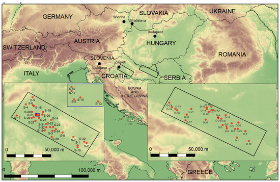
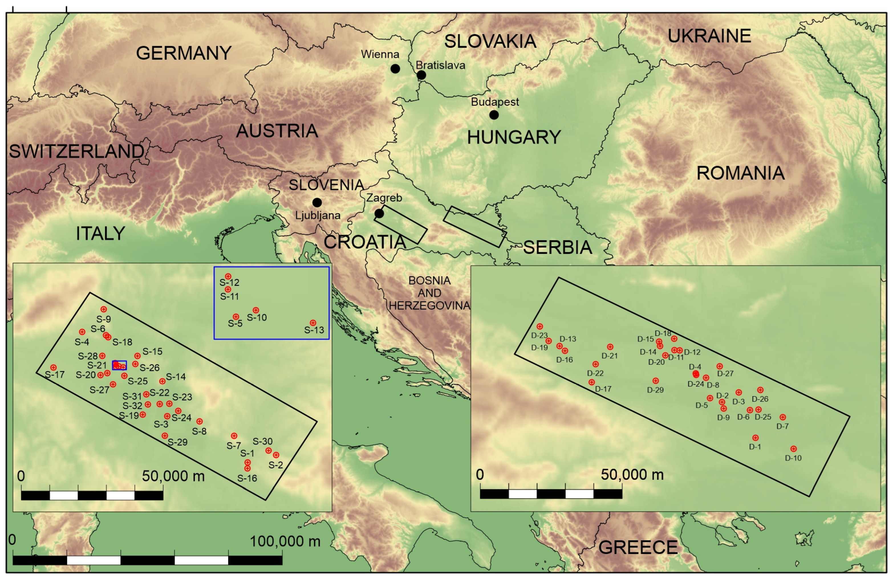
The locations of the wells included in this study are shown in Figure 2. Note that wells from the Sava Basin are designated as “S-number” (e.g., S-1, S-2), whereas wells from the Drava Basin are labeled as “D-number” (e.g., D-1, D-2).
Figure 2.
Well locations included in the research.
Since several sets of multiple temperature measurements were taken at different depths, in order to compare Tmax with uHPCT, it was necessary to estimate the HPCT at the bottom of the well. The geothermal gradient, Gg (°C/100 m), was determined by integrating the mean annual surface temperature (Tsurfavg) of 13.6 °C for the Sava Basin and 13.53 °C for the Drava Basin, the HPCT values, and the depths corresponding to multiple measurement intervals (HHPCT):
Gg = ((HPCT − Tsurfavg)/HHPCT) × 100
The geothermal gradient was also used to calculate the corrected temperature at the depth at which the drill-stem test (DST) was conducted in the same way as for HPCT values. This enabled a comparison of temperature values obtained from DSTs and the HPCTs.
In sedimentary basins characterized by relatively continuous sedimentation and a predominantly conductive heat-transfer regime, the assumption of a linear geothermal gradient represents a reasonable approximation at the regional scale (e.g., refs. [27,28]).
It should be noted that for the mean annual surface temperature (Tsurfavg), a value of mean annual ground temperature at the depth of 5 cm was used, corresponding to the Mean Annual Ground Surface Temperature (MAGST), as proposed by [29]. The value for the Sava Basin was obtained as an average calculated from measurements at stations in Kutina, Zagreb, and Sisak, while the value for the Drava Basin was derived from measurements at stations in Osijek, Valpovo, and Beli Manastir. Data were supplied by the Croatian Meteorological and Hydrological Service.
5. Results
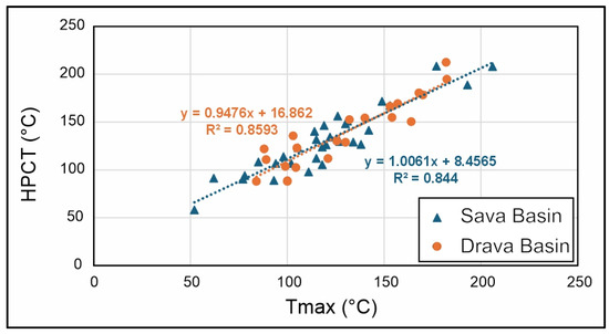
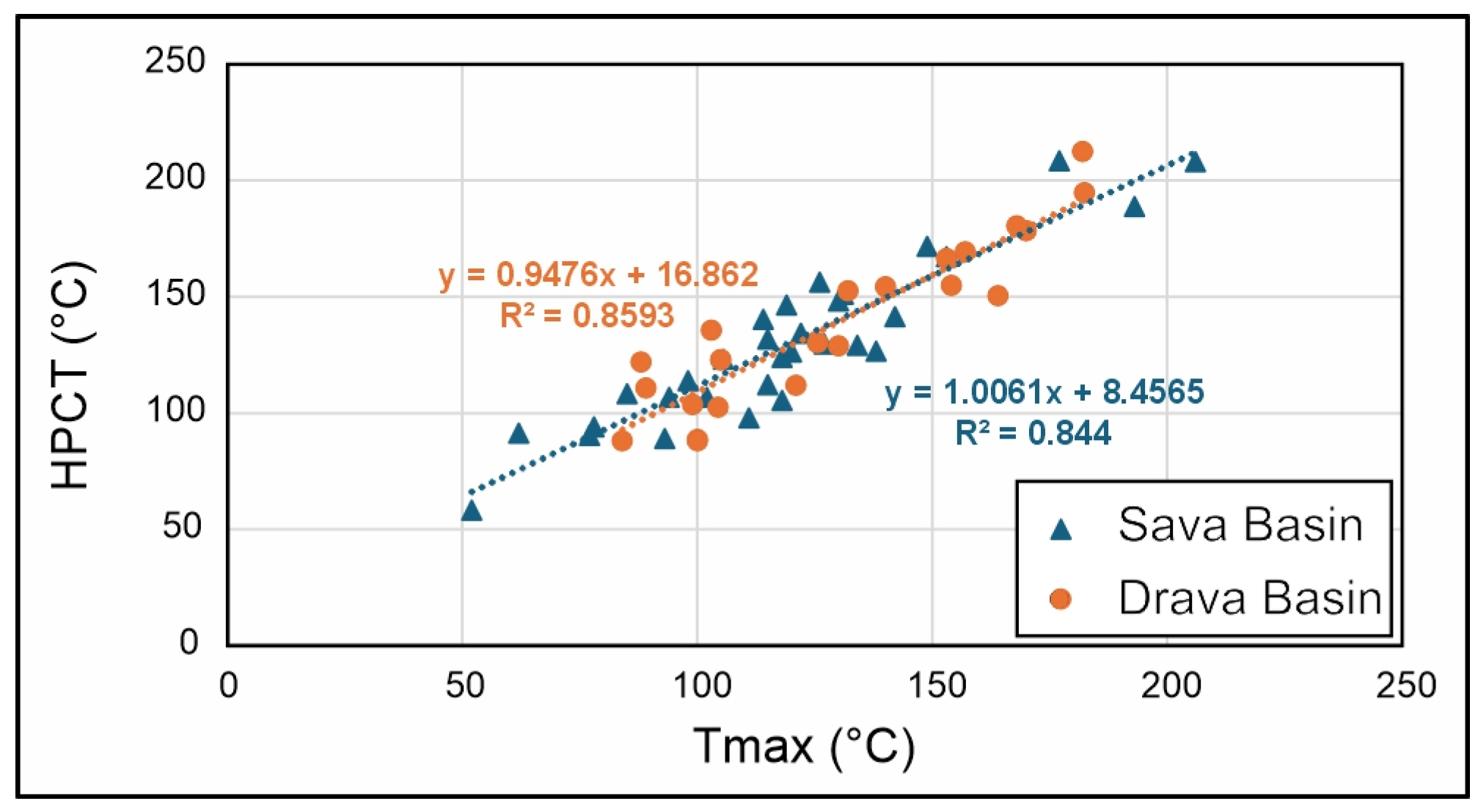
Figure 3 presents the correlation between Tmax and HPCT for the Sava and Drava Basins. The correlation for the Sava Basin is based on data from 31 wells and spans a broader range of temperature values. On the other hand, the correlation for the Drava subbasin is derived from temperature data obtained from 18 wells. The Tmax-HPCT correlation in the Sava Basin yields a slightly lower coefficient of determination (R2) of 0.844 compared to that of the Drava Basin, which is 0.8593. The correlation that includes data from both subbasins shows an intermediate R2 value of 0.8457, falling between those calculated individually for the Sava and Drava Basins.
Figure 3.
Tmax and HPCT relationship for both the Sava and Drava Basin.
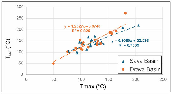
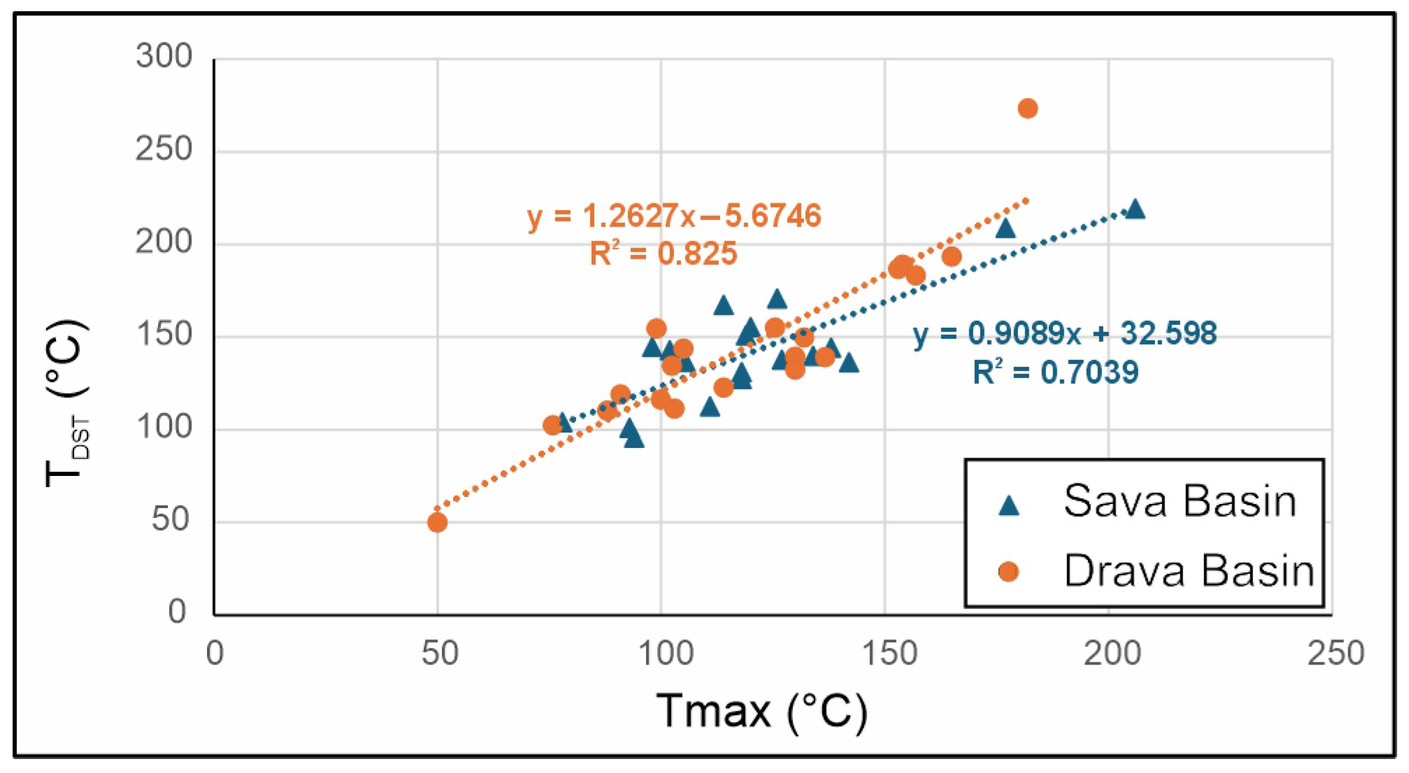
Figure 4 illustrates the correlation between Tmax and TDST for the Sava and Drava Basins. The number of input data for the Sava and Drava Basins is similar; correlation is based on data from 20 wells for the Sava and 21 wells for the Drava Basin. The Tmax–TDST correlation for the Sava Basin again yields a slightly lower coefficient of determination (R2 = 0.7039) compared to that of the Drava Basin (R2 = 0.825). Statistical significance (p value) as well as a standard error of estimate (SEE) are presented in Table 2.
Figure 4.
Tmax and TDST relationship for Sava and Drava Basins.
Table 2.
p-value of the regression coefficient and standard error of temperature estimate (SEE).
The Tmax-HPCT correlations show greater similarity between the Sava Basin and the Drava Basin than the Tmax-TDST correlations, where the difference between basins is more pronounced. For the Sava Basin, the increase in TDST with respect to Tmax rises with the rise in temperature values, i.e., the difference is more pronounced for higher temperature values. On the other hand, the regression line for the Sava Basin exhibits a gentler slope compared to the regression line for the Drava Basin. Slope analysis was performed based on the [30], which showed that there is no statistical difference in slope of the regression curve for the Sava and Drava Basins in both Tmax vs. HPCT (p = 0.62) and Tmax vs. TDST (p = 0.1).
Temperature values, including Tmax, HPCT and TDST, in the Sava Basin are given in Table 3. The table shows that temperatures at the total depth of the well, calculated using the geothermal gradient obtained from DST temperature data, exceed values of temperature calculated using the geothermal gradient obtained from Horner-plot-corrected temperature values in 18 wells, while they are lower in only two wells.
Table 3.
Temperature values for wells in Sava Basin.
The same comparison of HPCT and TDST in the Drava Basin is given in Table 4. It is evident that Tmax values exceed HPCT values in four wells, while they are lower than TDST values in all wells, except in the well D-26, where the Tmax and TDST values are the same. A comparison of the TDST and HPCT values shows that HPCT values are higher in only four wells in the Drava Basin, while they are lower in 12 wells.
Table 4.
Temperature values for Drava Basin.
6. Discussion
From the presented results it is evident that Tmax values are better correlated with HPCT than with TDST values. This is to be expected given the fact that the Horner correction method was developed to estimate the SFT based on non-equilibrium temperature values and it is expected that some of the thermal borehole effects are maintained even after the corrections. On the other hand, DST temperature measurements are expected to show specific thermal conditions and therefore their correlation with BHT is weaker because they are arguably approximating the SFT. Section 4 noted that the source of the reported Tmax values is not recorded in well documentation. In practice, Tmax may be derived from multiple sources, such as maximum temperatures from wireline logs, temperature maximums recorded during drill-stem tests, or even approximate values estimated during drilling. Each of these possible origins carries different implications and uncertainties. The stronger correlation observed between Tmax and HPCT values suggests that the Tmax measurements likely represent uncorrected, non-equilibrium temperature data. This is especially indicative of the Sava Basin, where the determination factor for Tmax-DST correlation is significantly higher (0.844) than for Tmax-TDST correlation (R2 = 0.7039). Also, it should be noted that even though Tmax values can be relatively well correlated with HPCT values, in most cases they significantly differ from HPCT values, and this fact is important to emphasize the unreliability of Tmax data in estimating subsurface temperature. Significant differences between Tmax and HPCT are found in most of the wells in the Sava Basin, where 19 out of 31 wells (61.3%) show a difference between Tmax and HPCT values exceeding 10 °C, and in seven wells the difference between Tmax and HPCT is higher than 20 °C. In the Drava Basin, in 14 out of 29 wells (48.3%), the differences between Tmax and HPCT values exceeding 10 °C are registered and in five wells the difference is higher than 20 °C.
The values of TDST are higher than HPCT values in most wells since DSTs are generally conducted at the bottom of the well, i.e., the tested formation corresponds to the target interval of the well. Thus, it may be reasonable to assume that the measured temperature does not exceed the actual formation temperature, so that it is in fact the closest approximation of the SFT [12]. However, if the DST is not performed at the bottom of the well, leaking through the bottom packer could arguably lead to higher measured temperatures than the SFT of the tested formation. Although this could happen at greater depths due to high temperatures affecting the sealing capability of packers in open holes [31], the effect would have to be very limited, since every leakage through the packer should be observed on pressure data.
Table 3 and Table 4 show that the TDST is higher than the HPCT in 17 out of 20 wells (85%) in the Sava Basin and 12 out of 15 wells (80%) in the Drava Basin, with a maximum difference of 61 °C (registered in well D-21, Table 4). This finding indicates that the classic Horner correction may systematically underestimate true formation temperatures. This is in accordance with Peters and Nelson (2012) [12], who stated that BHT data corrected using Horner’s method may still be systematically lower than true formation temperatures, as well as with the findings of Förster (2001) [9], who reported that corrected BHT values systematically underestimate actual formation temperatures.
It is obvious that there is a lack of data that can be used to estimate geothermal gradient. Namely, for 35.5% wells (11 out of 31) in the Sava Basin and 34.5% (10 out of 29) in the Drava Basin, there are no values of temperature recorded during the DST. This is mostly due [32] to the problems with packer leakage or the use of inadequate thermometers.
Not only is there a lack of subsurface data, as well as problems with the reliability of those data, but the ground surface temperature data could also be regarded as of limited reliability, since they are influenced by complex thermal interactions of different surface factors [33,34,35]. For example, the use of MAGST only somewhat eliminates the effect of snow cover in areas with a cold climate [32]. However, given that both areas are characterized by moderate climate, influences of surface factors, primarily snow cover and vegetation, are expected to be less pronounced.
The main limitation of the conducted study lies in fact that the temperature gradients were calculated using temperature data of different sources measured at different depths and these temperatures were extrapolated to the bottom of the well. In doing so, it is assumed that the geothermal gradient remains constant with depth, implying a linear increase in temperature with increasing depth. Such an assumption obviously simplifies temperature distribution in the subsurface and is not a realistic representation of the more complex thermal conditions. However, in the given circumstances, when there is a lack of data on temperature in the subsurface, the authors believe that this simplification is justified.
Temperature measurements in wells require careful consideration, particularly when evaluating the geothermal potential of a reservoir or a wider region. Discrepancies exceeding 20 °C between Horner-plot-corrected temperatures (HPCTs) and drill-stem test temperatures (TDST)—the latter generally regarded as the closest approximation to the static formation temperature (SFT)—may have significant implications for geothermal energy utilization strategies. Such differences can determine whether the resource is suitable for lower-enthalpy applications, such as greenhouse heating, or for higher-enthalpy use, including electricity generation in binary geothermal power plants.
The overall usefulness of legacy wells for the assessment of geothermal potential, even at the regional scale, is very limited. Temperature measurements obtained at a single point, such as bottom-hole temperature (BHT) measurements, even when repeated and therefore allowing for certain corrections, or those recorded within a limited interval (temperatures derived from drill-stem tests, DSTs), inevitably introduce significant uncertainties. These uncertainties relate both to the reliability of the measured temperature itself, but also to the limited capability for reliable spatial interpolation of this variable.
Although some authors [8] see the continuous temperature measurements (temperature logging) as an improved approach that would lead to more reliable assessments, it should be noted that in practice their reliability is often constrained by the insufficient time allowed for the borehole to re-establish thermal equilibrium after drilling operations. In this respect, the situation is frequently not substantially improved even in modern wells where temperature logging is routinely performed, as operational constraints rarely allow for the extended shut-in periods required for thermal equilibrium.
Consequently, geothermal assessments based on such datasets should be interpreted with caution. Significant improvements in data quality are difficult to achieve in practice, as maintaining wells in a shut-in state for sufficiently long periods is associated with considerable operational costs.
7. Conclusions
Although the error in temperature data from deep wells (BHT and Tmax) is generally well recognized, the application of any temperature corrections will also result in an error. The comparison of corrected temperature data and temperature data derived from drill-stem tests (TDST) can arguably be used to establish the amount of the error.
This study provides the first basin-scale empirical assessment of the reliability of reported Tmax values for subsurface temperature estimation and introduces a regression-based approach for recalibrating Tmax using DST measurements, improving geothermal resource evaluation accuracy.
The study indicates that the reported maximum temperature values (Tmax) for deep exploration wells in the Sava and Drava Basins differ from both Horner-corrected temperatures (HPCT) and those recorded during drill-stem tests (TDST). In most cases, these reported values are not true maxima, as they are typically lower than both HPCT and TDST measurements.
Particular attention should be paid to discrepancies exceeding 20 or 30 °C between Horner-corrected temperatures (HPCTs) and drill-stem test temperatures (TDST), the latter generally considered the most reliable proxy for static formation temperature (SFT). If not adequately recognized and addressed, such discrepancies may result in significant misestimation of subsurface thermal conditions. These inaccuracies can lead to inappropriate classification of geothermal resources and misleading decisions regarding their technical and economic utilization. This issue is of particular relevance in the context of ongoing and planned geothermal development within the Sava and Drava Basins, where the reliability of subsurface temperature models is fundamental for reducing exploration risk and ensuring the long-term sustainability of geothermal resource utilization. Given that low- to medium-temperature hydrothermal reservoirs are expected in these regions, a temperature discrepancy on the order of 20 °C represents a significant deviation. This is especially critical because a minimum wellhead temperature of approximately 80 °C constitutes the lower operational limit for the deployment of Organic Rankine Cycle (ORC) systems [36]. Consequently, an underestimation of reservoir temperature to this threshold would lead to the erroneous exclusion of a potentially viable geothermal resource from consideration for electricity generation using ORC technology. The procedure described in this study is applicable to regional-scale investigations of sedimentary basins with diverse geological characteristics, provided that subsurface heat transfer is dominated by conduction. The use of a linear geothermal gradient makes the approach unsuitable for local-scale temperature assessments, since the deviations from linearity are expected to occur due to lithological heterogeneities, variations in thermal conductivity, and fault-related heat advection.
Author Contributions
Conceptualization, I.K.M.; methodology, I.K.M.; software, M.C.; validation, I.K.M. and M.C.; formal analysis, Z.S., A.P. and I.K.M.; investigation, I.K.M., A.P. and Z.S.; data curation, I.K.M. and M.C.; writing—original draft preparation, I.K.M.; writing—review and editing, M.C.; visualization, I.K.M. and M.C.; supervision, I.K.M.; project administration, M.C.; funding acquisition, M.C. All authors have read and agreed to the published version of the manuscript.
Funding
This work has been supported by the Next Generation NPOO project (581100006–GEPARD Recovery and Resilience Mechanism), funded by the European Union and by Croatian Science Foundation (No. HRZZ UIP-2019-04-3846): “GEOlogical characterization of the Eastern part of the Drava depression subsurface intended for the evaluation of Energy Potentials (GEODEP)”.
Data Availability Statement
Original research data can be obtained from the Croatian Hydrocarbon Agency for academic research.
Acknowledgments
The authors would like to extend their gratitude to Schlumberger company for generously donating the Petrel 2024 academic software license. Additionally, we acknowledge the Croatian Hydrocarbon Agency for granting permission to access the data, without which the analysis presented in this paper would not have been possible. The authors would also like to thank the Croatian Meteorological and Hydrological Service for providing annual ground temperature data. The authors would also acknowledge the efforts of four anonymous reviewers in improving the manuscript.
Conflicts of Interest
The funders had no role in the design of the study; in the collection, analyses, or interpretation of data; in the writing of the manuscript; or in the decision to publish the results.
Abbreviations
The following abbreviations are used in this manuscript:
| Tmax | Maximum temperature value |
| HPCT | Horner-corrected temperature |
| HHPCT | Multiple measurement interval |
| TDST | Temperature recorded during drill-stem test |
| BHT | Bottom-hole temperature |
| SFT | Static Formation Temperature |
| Tcorr | Corrected temperature value |
| Gg | Geothermal gradient |
| Tsurfavg | Mean annual surface temperature |
References
- Chambers, E.L.; Bonadio, R.; Fullea, J.; Lebedev, S.; Xu, Y.; Kiyan, D.; Bean, C.J.; Meere, P.A.; Mather, B.; O’Reilly, B.M. Determining Subsurface Temperature & Lithospheric Structure from Joint Geophysical-Petrological Inversion: A Case Study from Ireland. Tectonophysics 2023, 869, 230094. [Google Scholar] [CrossRef] [Scilit]
- Schumacher, S.; Moeck, I. A New Method for Correcting Temperature Log Profiles in Low-Enthalpy Plays. Geotherm. Energy 2020, 8, 27. [Google Scholar] [CrossRef] [Scilit]
- Waples, D.W.; Pedersen, M.R.; Kuijpers, P. Correction of Single Log-Derived Temperatures in the Danish Central Graben, North Sea. Nat. Resour. Res. 2004, 13, 229–239. [Google Scholar] [CrossRef] [Scilit]
- Sekiguchi, K. A Method for Determining Terrestrial Heat Flow in Oil Basinal Areas. Tectonophysics 1984, 103, 67–79. [Google Scholar] [CrossRef] [Scilit]
- Bullard, E.C. The Time Necessary for a Bore Hole to Attain Temperature Equilibrium. Geophys. J. Int. 1947, 5, 127–130. [Google Scholar] [CrossRef] [Scilit]
- Aabø, T.M.; Hermanrud, C. Toward a Global Model for Correction of Bottomhole Temperature Data: Progress and Limitations. AAPG Bull. 2019, 103, 139–155. [Google Scholar] [CrossRef] [Scilit]
- Dowdle, W.L.; Cobb, W.M. Static Formation Temperature from Well Logs—An Empirical Method. J. Pet. Technol. 1975, 27, 1326–1330. [Google Scholar] [CrossRef] [Scilit]
- Zhan, W.; Chen, Y.; Liu, Q.; Li, J.; Sacchi, M.D.; Zhuang, M.; Liu, Q.H. Simultaneous Prediction of Petrophysical Properties and Formation Layered Thickness from Acoustic Logging Data Using a Modular Cascading Residual Neural Network (MCARNN) with Physical Constraints. J. Appl. Geophys. 2024, 224, 105362. [Google Scholar] [CrossRef] [Scilit]
- Förster, A. Analysis of Borehole Temperature Data in the Northeast German Basin: Continuous Logs versus Bottom-Hole Temperatures. Pet. Geosci. 2001, 7, 241–254. [Google Scholar] [CrossRef] [Scilit]
- Rider, M. The Geological Interpretation of Well Logs, 2nd ed.; Rider-French Consulting Ltd.: Sutherland, UK, 2002. [Google Scholar]
- Hermanrud, C.; Lerche, I.; Meisingset, K.K. Determination of Virgin Rock Temperature from Drillstem Tests. J. Pet. Technol. 1991, 43, 1126–1131. [Google Scholar] [CrossRef] [Scilit]
- Peters, K.E.; Nelson, P.H. Criteria to Determine Borehole Formation Temperatures for Calibration of Basin and Petroleum System Models. In Analyzing the Thermal History of Sedimentary Basins: Methods and Case Studies; SEPM (Society for Sedimentary Geology): Claremore, OK, USA, 2012; pp. 5–15. [Google Scholar]
- Horner, D.R. Pressure Build-up in Wells. In Proceedings of the Third World Petroleum Congress, The Hague, The Netherlands, 28 May–6 June 1951; pp. 503–521. [Google Scholar]
- Ascencio, F.; Samaniego, F.; Rivera, J. Application of a Spherical-Radial Heat Transfer Model to Calculate Geothermal Gradients from Measurements in Deep Boreholes. Geothermics 2006, 35, 70–78. [Google Scholar] [CrossRef] [Scilit]
- Waples, D.W.; Ramly, M. A Statistical Method for Correcting Log-Derived Temperatures. Pet. Geosci. 2001, 7, 231–240. [Google Scholar] [CrossRef] [Scilit]
- Goutorbe, B.; Lucazeau, F.; Bonneville, A. Comparison of Several BHT Correction Methods: A Case Study on an Australian Data Set. Geophys. J. Int. 2007, 170, 913–922. [Google Scholar] [CrossRef] [Scilit]
- Hasan, A.R.; Kabir, C.S. Static Reservoir Temperature Determination from Transient Data After Mud Circulation. SPE Drill. Complet. 1994, 9, 17–24. [Google Scholar] [CrossRef] [Scilit]
- Rangel-Arista, J.A.; Zarrouk, S.J.; Kaya, E. Temperature Transient Analysis: Static Formation Temperature Test (SFTT) an Overview. Geothermics 2024, 122, 103058. [Google Scholar] [CrossRef] [Scilit]
- Matenco, L.; Radivojević, D. On the Formation and Evolution of the Pannonian Basin: Constraints Derived from the Structure of the Junction Area between the Carpathians and Dinarides. Tectonics 2012, 31, TC6007. [Google Scholar] [CrossRef] [Scilit]
- Ádám, A.; Bielik, M. The Crustal and Upper-Mantle Geophysical Signature of Narrow Continental Rifts in the Pannonian Basin. Geophys. J. Int. 1998, 134, 157–171. [Google Scholar] [CrossRef] [Scilit]
- Lenkey, L.; Dövényi, P.; Horváth, F.; Cloetingh, S.A.P.L. Geothermics of the Pannonian Basin and Its Bearing on the Neotectonics. EGU Stephan Mueller Spec. Publ. Ser. 2002, 3, 29–40. [Google Scholar] [CrossRef] [Scilit]
- Horváth, F.; Cloetingh, S. Stress-Induced Late-Stage Subsidence Anomalies in the Pannonian Basin. Tectonophysics 1996, 266, 287–300. [Google Scholar] [CrossRef] [Scilit]
- Prelogović, E.; Saftić, B.; Kuk, V.; Velić, J.; Dragaš, M.; Lučić, D. Tectonic Activity in the Croatian Part of the Pannonian Basin. Tectonophysics 1998, 297, 283–293. [Google Scholar] [CrossRef] [Scilit]
- Miocic, J.; Heinemann, N.; Edlmann, K.; Scafidi, J.; Molaei, F.; Alcalde, J. Underground Hydrogen Storage: A Review. Geol. Soc. Lond. Spec. Publ. 2023, 528, 73–86. [Google Scholar] [CrossRef] [Scilit]
- Li, R.; Kockelman, K.M.; Lee, J. Reducing Greenhouse Gas Emissions from Long-Distance Business Travel: How Far Can We Go? Transp. Res. Rec. J. Transp. Res. Board 2022, 2676, 472–486. [Google Scholar] [CrossRef] [Scilit]
- Buonocore, J.J.; Salimifard, P.; Magavi, Z.; Allen, J.G. Inefficient Building Electrification Will Require Massive Buildout of Renewable Energy and Seasonal Energy Storage. Sci. Rep. 2022, 12, 11931. [Google Scholar] [CrossRef] [Scilit] [PubMed]
- Christie, C.H.; Nagihara, S. Geothermal Gradients of the Northern Continental Shelf of the Gulf of Mexico. Geosphere 2016, 12, 26–34. [Google Scholar] [CrossRef] [Scilit]
- Hu, K.; Chen, Z.; Issler, D.R. Determination of Geothermal Gradient from Borehole Temperature and Permafrost Base for Exploration Wells in the Beaufort-Mackenzie Basin; Natural Resources Canada: Ottawa, ON, Canada, 2014. [Google Scholar]
- Kolawole, F.; Evenick, J.C. Global Distribution of Geothermal Gradients in Sedimentary Basins. Geosci. Front. 2023, 14, 101685. [Google Scholar] [CrossRef] [Scilit]
- Andrade, J.M.; Estévez-Pérez, M.G. Statistical Comparison of the Slopes of Two Regression Lines: A Tutorial. Anal. Chim. Acta 2014, 838, 1–12. [Google Scholar] [CrossRef] [Scilit]
- Ringgenberg, P.; Self, J.C. Increased Reliability For HP/HT Drill Stem Testing from Full Scale Tool Tests. In Proceedings of the Offshore Technology Conference, OTC, Houston, TX, USA, 6–9 May 1996. [Google Scholar]
- Goodrich, L.E. The Influence of Snow Cover on the Ground Thermal Regime. Can. Geotech. J. 1982, 19, 421–432. [Google Scholar] [CrossRef] [Scilit]
- Luo, D.; Jin, H.; Bense, V.F. Ground Surface Temperature and the Detection of Permafrost in the Rugged Topography on NE Qinghai-Tibet Plateau. Geoderma 2019, 333, 57–68. [Google Scholar] [CrossRef] [Scilit]
- Luo, D.; Jin, H.; Marchenko, S.S.; Romanovsky, V.E. Difference between Near-Surface Air, Land Surface and Ground Surface Temperatures and Their Influences on the Frozen Ground on the Qinghai-Tibet Plateau. Geoderma 2018, 312, 74–85. [Google Scholar] [CrossRef] [Scilit]
- Guglielmin, M. Ground Surface Temperature (GST), Active Layer and Permafrost Monitoring in Continental Antarctica. Permafr. Periglac. Process. 2006, 17, 133–143. [Google Scholar] [CrossRef] [Scilit]
- Zhai, H.; An, Q.; Shi, L.; Lemort, V.; Quoilin, S. Categorization and Analysis of Heat Sources for Organic Rankine Cycle Systems. Renew. Sustain. Energy Rev. 2016, 64, 790–805. [Google Scholar] [CrossRef] [Scilit]

Disclaimer/Publisher’s Note: The statements, opinions and data contained in all publications are solely those of the individual author(s) and contributor(s) and not of MDPI and/or the editor(s). MDPI and/or the editor(s) disclaim responsibility for any injury to people or property resulting from any ideas, methods, instructions or products referred to in the content. |
© 2026 by the authors. Licensee MDPI, Basel, Switzerland. This article is an open access article distributed under the terms and conditions of the Creative Commons Attribution (CC BY) license.