Long-Tailed Mineral Identification Based on Multi-Stage Training

Abstract

Deep learning-based mineral image recognition from macroscopic hand-specimen photographs has emerged as an important approach for mineral identification. However, the inherent imbalance in the natural distribution and reserves of minerals leads to a long-tailed distribution in mineral image datasets, resulting in significantly lower recognition accuracy for minerals with fewer images. To address this issue, we propose a multi-stage training framework that enhances the recognition performance of tail-class minerals through feature extractor adjustment, core feature learning, and classifier re-training. Feature extractor adjustment increases the logit scores of tail-class samples, core feature learning increases the sampling frequency of low-confidence instances, and classifier re-training increases the classifier’s sensitivity to tail-class instances. The multi-stage training framework improves the overall performance of mineral recognition and strengthens the model’s generalization ability. Experimental results on a dataset of 36 mineral categories demonstrate that the proposed method increases the mean accuracy of the one-third mineral species with the least amount of data from 67.47% to 80.06%, with a maximum improvement of 24.1%. Moreover, the overall mean accuracy across all 36 mineral categories increases from 77.27% to 81.27%, confirming the effectiveness of the proposed approach.

1. Introduction

Mineral resources are fundamental for modern society, and borehole sections, geological sections, geophysical/geochemistry observations, and satellite/remote-sensing data have been combined for mineral exploration [1,2,3,4]. However, the above methods are time-consuming and costly. In recent years, deep learning-based approaches have been demonstrated as fast and economical for mineral recognition from macroscopic hand-specimen photographs, which will be helpful in mineral exploration [5,6]. For example, Peng et al. [7] and Li et al. [8] used the Inception-V3 network to identify the minerals. Asiedu et al. [9] designed MiNet, which successfully identified seven mineral categories, validating the practicality of the CNN (Convolutional Neural Network) for mineral recognition. Theerthagiri et al. [10] further demonstrated the efficiency of residual networks by integrating multi-pooling algorithms with models such as VGG and ResNet. Li et al. [11] employed a ConvNeXt network on a 26-class mineral dataset, indicating the effectiveness of self-attention. Jia et al. [12] introduced the SwinMin model on a dataset with 45 mineral categories and further demonstrated the potential of attention mechanisms for mineral image recognition. He et al. [13] employed YOLOv8 to identify the minerals that may exist with other items, such as introductory cards. Multimodal frameworks have been developed to solve the problem of difficulty in distinguishing different minerals that may have the same visual characteristics [14,15,16]. However, these methods largely overlook the inherent data imbalance present in mineral image datasets [17,18,19, 20].

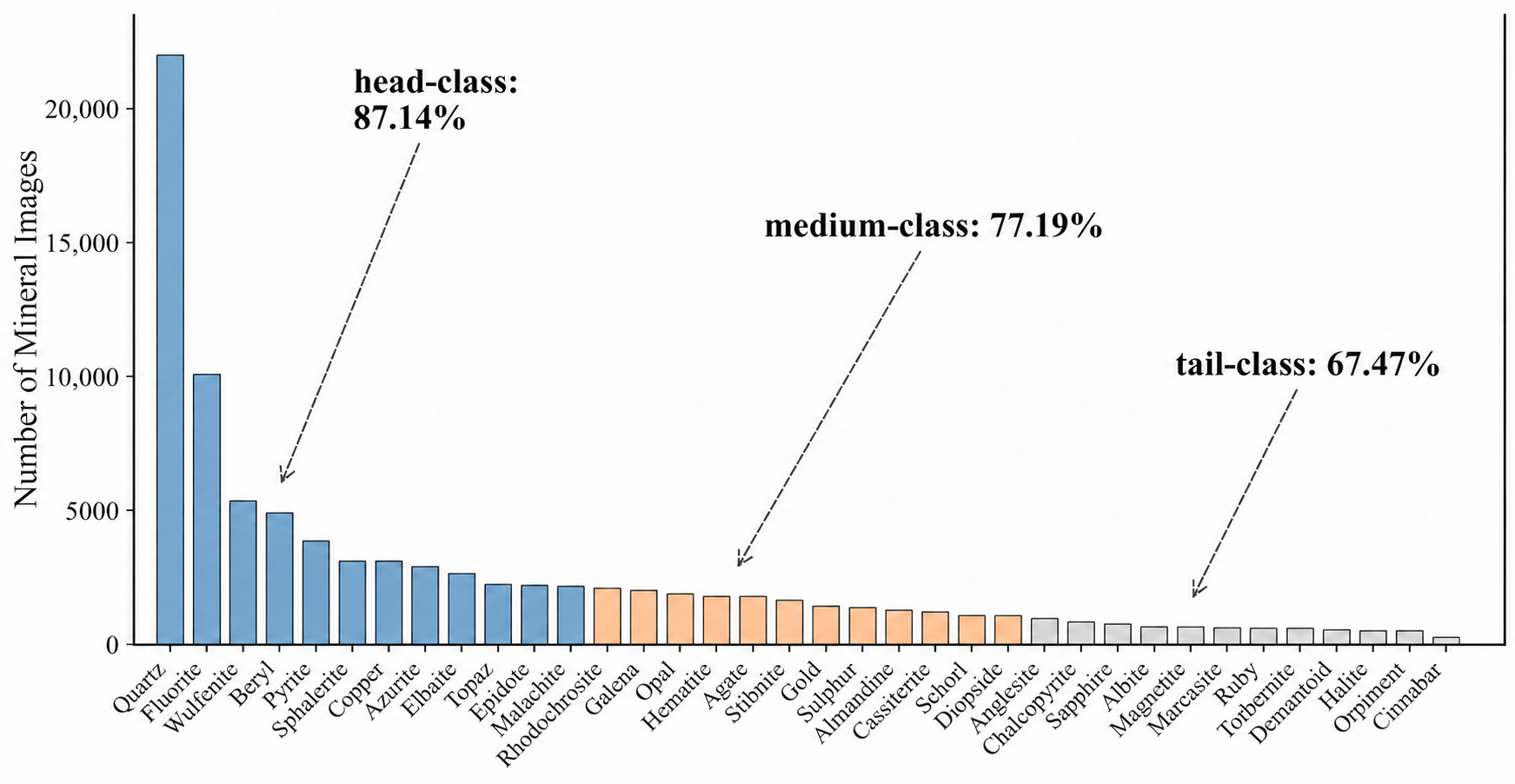
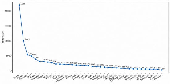
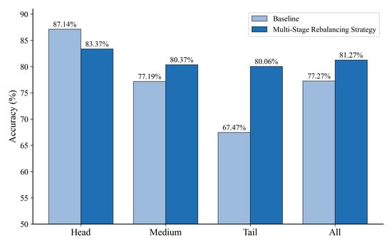
Due to the uneven natural distribution and varying reserves of different minerals, the resulting image datasets are typically long-tailed [10,21]: common minerals (e.g., quartz or calcite) are well-represented, whereas rare minerals (e.g., certain gemstones or specialty minerals) suffer from a severe lack of samples. As shown in Figure 1, although ResNet-50 achieves an overall recognition accuracy of 77.27% on the Minerals-36 dataset [14,15,16], the average accuracy for head-class minerals (top one-third in sample count) reaches 87.14%, while the medium-class minerals drop to 77.19%, and the tail-class minerals (bottom one-third) perform significantly worse, with a mean accuracy of only 67.47%.

Figure 1. Long-tailed distribution of mineral images.

Data imbalance in mineral image recognition can be addressed through under-sampling or over-sampling. However, under-sampling reduces the number of head-class samples, potentially degrading their recognition accuracy, while over-sampling compensates for the lack of tail-class samples by repeating them, offering no new features and potentially leading to overfitting [22]. Recent long-tailed recognition studies have also improved tail-class representation through head-to-tail feature fusion and category extrapolation, while decoupled backbone-classifier learning has been revisited in long-tailed dataset distillation [23,24,25]. More recently, decision-boundary-aware generation has been proposed to reduce inter-class overlap and improve tail-class separability by generating informative near-boundary samples [26]. These developments further support the importance of improving tail-class feature diversity and reducing optimization bias. Therefore, it is imperative to go beyond simply adjusting sample quantities and instead guide the model to learn more representative features of tail-class minerals during training.

To address the challenges posed by sample imbalance in mineral recognition, we propose a multi-stage rebalancing strategy that operates across different phases of the training process. At the feature extraction stage, the loss function is adjusted based on class sample frequencies [27,28], encouraging the model to sufficiently learn features of underrepresented classes rather than neglecting them due to their scarcity. To mitigate intra-class attribute imbalance, we adopt diversified sampling strategies [29] to ensure comprehensive coverage of both typical and rare attribute instances, and introduce additional constraints [30] to guide the model in focusing on the essential characteristics of each class, thereby enhancing recognition robustness under varying visual conditions. Finally, the parameters of the feature extractor are fixed, and the classifier is re-trained to correct classification biases [31], further balancing the model’s decision boundaries.

2. Materials and Methods

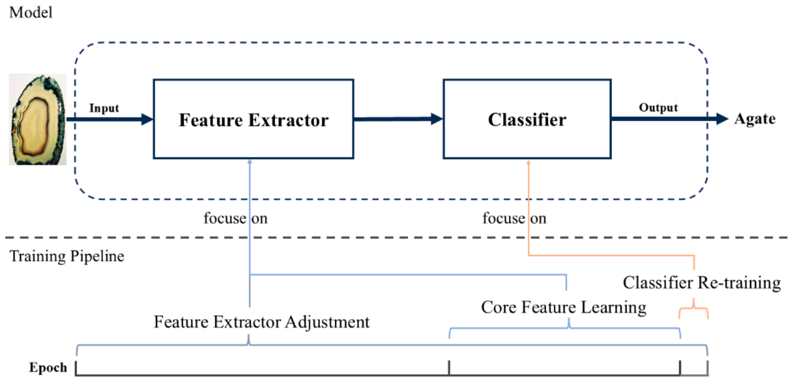
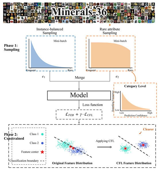
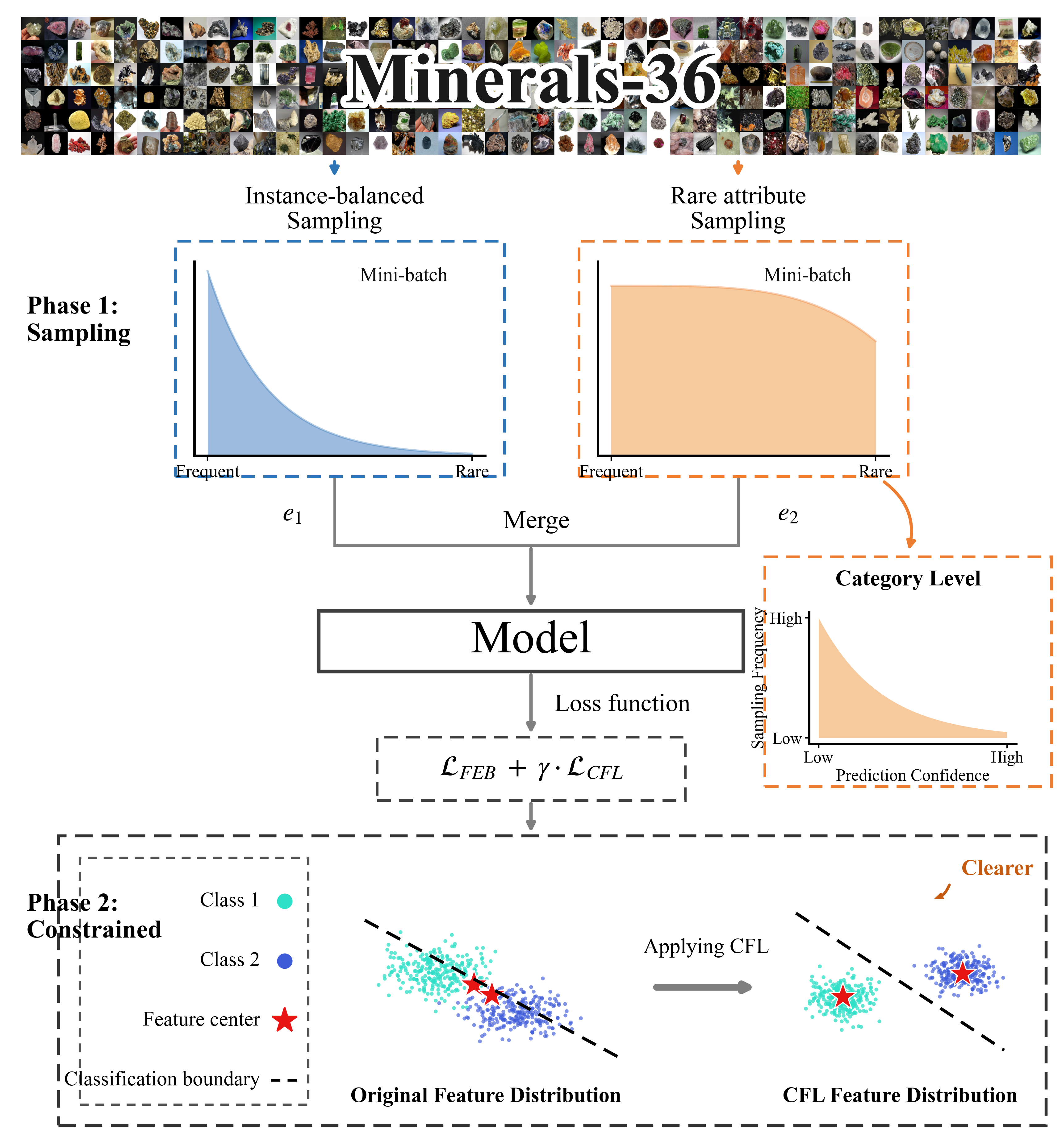
To address the issue of low average recognition accuracy caused by data imbalance in mineral image datasets, we propose a multi-stage rebalancing strategy, as illustrated in Figure 2. This strategy consists of three key components: feature extractor adjustment throughout the training process, core feature learning to address intra-class attribute imbalance in the later training phase, and classifier re-training at the final stage.

Figure 2. Multi-stage rebalancing strategy.

2.1. Feature Extractor Balancing

Feature extractor balancing (FEB) modifies the standard softmax cross-entropy loss [25] function (Equation (1)) into a frequency-aware loss function $ℒ$_FEB, as shown in Equation (2). This modification relatively increases the logit scores of tail-class samples, thereby enhancing the model’s ability to recognize tail-class minerals [27].

$${\mathcal{L}}_{\mathit{SCE}}=-\mathit{log}{\displaystyle \frac{e^{f_y\left(x\right)}}{{\displaystyle {\sum }_{y^{\prime }=1}^C}{e}^{f_{y^{\prime }}\left(x\right)}}}=\mathit{log}\left[1+{\displaystyle \sum _{y^{\prime }=1,y^{\prime }\ne y}^C}{e}^{f_{y^{\prime }}\left(x\right)-f_y\left(x\right)}\right]$$

(1)

$${\mathcal{L}}_{\mathit{FEB}}=-\mathit{log}{\displaystyle \frac{e^{f_y\left(x\right)+\mathit{log}{\pi }_y}}{{\displaystyle {\sum }_{y^{\prime }=1}^C}{e}^{f_{y^{\prime }}\left(x\right)+\mathit{log}{\pi }_{y^{\prime }}}}}=\mathit{log}\left[1+{\displaystyle \sum _{y^{\prime }=1,y^{\prime }\ne y}^C}{e}^{f_{y^{\prime }}\left(x\right)-f_y\left(x\right)+\mathit{log}\left(\frac{{\pi }_{y^{\prime }}}{{\pi }_y}\right)}\right]$$

(2)

In Equation (1), f_y(x) represents the model’s score for predicting the input mineral image x as its ground-truth class y, while $f_{y^{\prime }}\left(x\right)$ denotes the scores for other classes y′. The frequency-aware loss in Equation (2) adjusts each class score by adding a class-dependent term logπ_y, where π_y is the relative frequency of class y in the training set. In Equations (1) and (2), C is the number of mineral categories, that is, 36 in this work.

From Equation (2), when a tail-class mineral image is input to the model, its class frequency π_y is small (i.e., π_y ∼ 0), while other class frequencies ${\pi }_{y^{\prime }}\sim 1$. This leads to a positive value for $\log \left({\displaystyle \frac{{\pi }_{y^{\prime }}}{{\pi }_y}}\right)$, which increases the loss for tail-class minerals and amplifies their gradients. As a result, tail-class minerals exert a stronger influence on the model parameter updates during training [32]. Conversely, when head-class minerals are input, the term $\log \left({\displaystyle \frac{{\pi }_{y^{\prime }}}{{\pi }_y}}\right)$ becomes negative, thereby diminishing the dominant influence of head minerals in training. As illustrated in Figure 3, taking the tail-class mineral Albite as an example, its final training loss without adjustment was 8.06 × 10⁻⁵. After applying the feature extractor adjustment, the loss increased significantly to 4.95 × 10⁻². This forces the model to assign higher scores to Albite samples in order to reduce the loss [33], thereby encouraging more comprehensive feature learning for tail-class minerals.

Figure 3. Feature extractor adjustment (sample shown: Albite, a tail-class mineral in the dataset).

As shown in Figure 2, the adjusted loss function is employed throughout the training process to reinforce feature learning for tail minerals and improve their recognition performance [34].

2.2. Core Feature Learning for Intra-Class Attribute Imbalance

In Section 2.1, the mineral recognition model is trained using instance-balanced sampling, as illustrated on the left side of Figure 4. This approach samples each instance with equal probability to form a training subset e₁, which retains the original long-tailed distribution of the dataset. Although the feature extractor balancing in Section 2.1 enhances recognition performance for tail classes, the intra-class imbalance within each category still leads to suboptimal recognition accuracy for tail-class minerals [29,30].

Figure 4. Core feature learning of minerals.

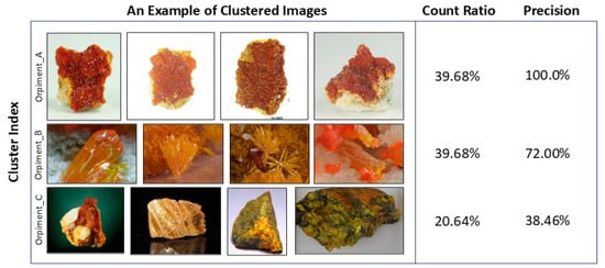
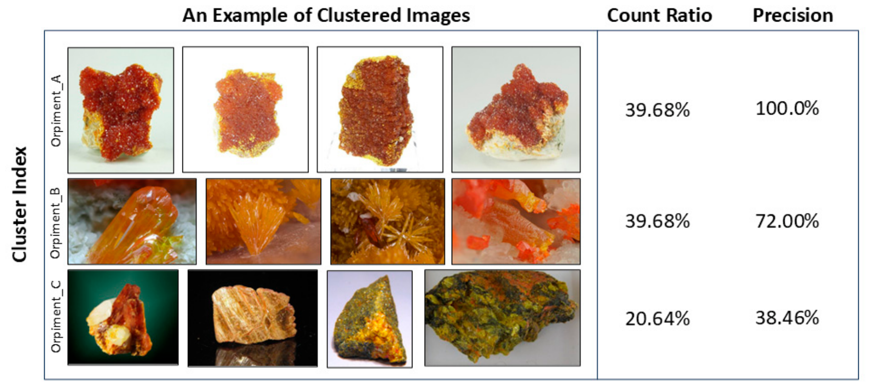
To investigate intra-class imbalance, we performed k-means clustering on the orpiment samples in our dataset. Orpiment is used as an example because it is a typical intra-class imbalance class, where minerals of this same category may have different color, transparency, and crystal habit. After k-means clustering, three distinct feature clusters are identified, as shown in Figure 5. These clusters group mineral images based on visual attributes and exhibit significant differences in recognition accuracy (100%, 72%, and 38.46%, respectively), which are positively correlated with the number of images in each cluster. This observation indicates that even within a single mineral category, subgroups with fewer samples suffer from poor recognition performance [35]. To address this, we introduce a core feature learning (CFL) strategy [29] that increases the sampling frequency of low-confidence instances, thereby improving their recognition accuracy.

Figure 5. Intra-class clustering results of the orpiment class in the dataset.

CFL assigns each mineral image an inverse-probability-based sampling weight s_i, as defined in Equation (3), and imposes a center loss constraint [36] (Equation (4)) to guide the model in learning core features that remain stable across varying visual attributes. This reduces the impact of non-core features and improves the model’s generalization capability [37].

$$s_i={\displaystyle \frac{{(1-p_i)}^{\beta }}{{\displaystyle {\sum }_{j=1}^{I_C}}{(1-p_j)}^{\beta }}},\beta ={\displaystyle \frac{\log \left(4\right)}{\log \left(\alpha \right)}},\alpha ={\displaystyle \frac{{\mu }_{\mathit{tail}}}{{\mu }_{\mathit{head}}}}$$

(3)

In Equation (3), p_i denotes the prediction confidence for image i in the previous training epoch; I_C is the number of images belonging to the class of image i; α is the ratio of the average prediction confidence of the least-confident 80% of samples in the class (μ_tail) to that of the most-confident 20% (μ_head), which is updated every training epoch during the activation window; β is the mapping exponent that ensures the least-confident 80% of images receive an increased sampling frequency. These re-weighted samples form an auxiliary training subset e₂, and are combined with e₁ to construct each training batch, ensuring a balanced representation of both typical and rare visual attributes.

In addition to the loss function $ℒ$_FEB described in Section 2.1, the training phase incorporates a center loss term $ℒ$_CFL (Equation (4)) to encourage convergence toward class-specific feature centers, leading to the overall loss formulation in Equation (5).

$${\mathcal{L}}_{\mathit{CFL}}={\displaystyle \sum _{i=1}^{{|e}_1|+|e_2|}}{‖f\left(x_i^e;\theta \right)-C_{y_i}‖}_2$$

(4)

$ℒ$ = $ℒ$_FEB + γ∙$ℒ$_CFL

(5)

Here, θ denotes the learnable parameters of the feature extractor, and $f\left(x_i^e;\theta \right)$ is the feature representation of sample $x_i^e$. The term $C_{y_i}$ is the centroid of features for class y_i, calculated as the mean feature vector of that class. Equation (4) computes the Euclidean distance between a sample’s feature and its corresponding class center. By minimizing $ℒ$_CFL, the model is encouraged to extract more consistent and representative features for each class. In Equation (5), γ is a hyperparameter that balances the contributions of the two loss components; a larger γ indicates stronger enforcement of the center constraint.

As shown in Figure 2, the core feature learning component is activated in the later stage of the feature learning phase. This design reflects the training dynamics: during early training, the model primarily learns general features shared across classes, and the center-based constraint is therefore introduced only after the representation has become more stable. As training progresses, the model gradually shifts focus toward class-specific core features. This transition reduces reliance on unstable or non-representative features, improves robustness against rare visual attributes, and enhances the model’s generalization capability.

2.3. Classifier Re-Training

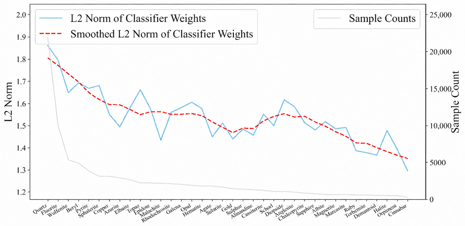
The feature extractor learning in Section 2.1 enables more balanced learning across different mineral categories, while the core feature learning in Section 2.2 facilitates the extraction of representative features within each category. However, as shown in Figure 6, the L2 norm of the classifier weight vectors after training in Section 2.1 and Section 2.2 remains correlated with the number of images per mineral class. Specifically, categories with more samples tend to have larger classifier weights, whereas those with fewer samples correspond to smaller weights. This imbalance results in a higher likelihood of tail-class mineral images being misclassified as head-class minerals, indicating the need to increase the classifier’s sensitivity to tail-class instances [38,39].

Figure 6. The L2 norm of the classifier weight vectors.

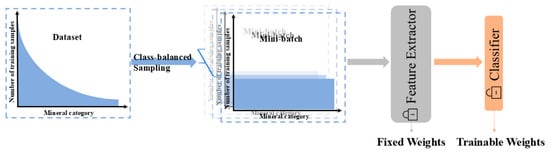
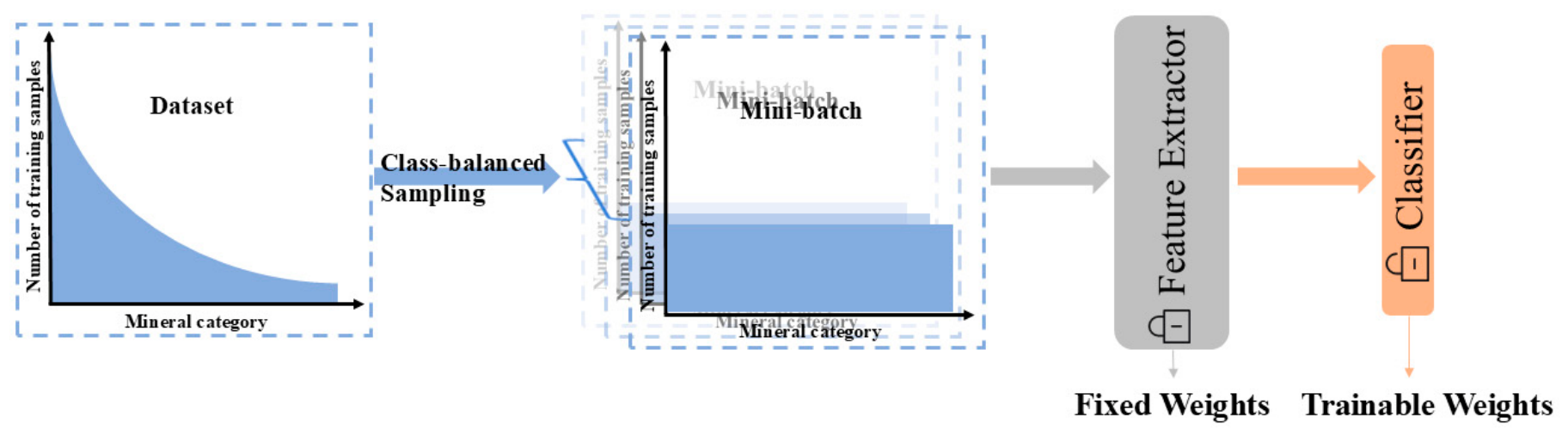
To address this issue, we employ classifier re-training (cRT) [31], as illustrated in Figure 7, after completing the training described in Section 2.1 and Section 2.2. During this final stage, the parameters of the feature extractor are frozen, and only the classifier is fine-tuned.

Figure 7. Classifier re-training.

In the re-training phase, we adopt class-balanced sampling, where each category is sampled with an equal probability of 1/C (where C denotes the number of mineral categories). This strategy ensures that minority classes receive the same level of attention as majority classes during training [40], thereby preventing the dominance of head-class minerals in shaping the classifier’s decision boundaries.

As depicted in Figure 2, classifier re-training is applied at the end of the multi-stage training pipeline. To maintain continuity in the training objective, we continue to use the loss function defined in Equation (2). However, since the classifier re-training phase differs from the intra-class sampling strategy employed in core feature learning, we omit the center constraint loss defined in Equation (5). By decoupling the training of the feature extractor and the classifier, this approach effectively resolves the imbalance in classifier decision boundaries that may arise during joint training. As a result, it enhances the model’s recognition performance, particularly on tail-class minerals.

3. Results

In this section, we present a series of experiments to evaluate the effectiveness of the proposed method.

3.1. Dataset and Evaluation Metrics

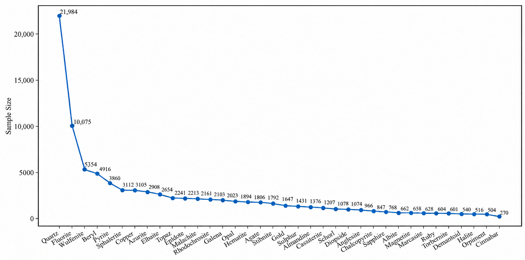
The dataset used in this study, Minerals-36, is an enhanced version of the datasets employed in [14,15,16]. The mineral images were primarily collected via web crawling from the Mindat website, followed by manual filtering to remove low-quality samples, ensuring the accuracy and domain relevance of the dataset. Minerals-36 comprises a total of 113,569 images spanning 36 mineral categories. The distribution of image counts per category, as shown in Figure 8, exhibits a clear long-tailed pattern. The dataset is randomly split into training, validation, and test sets in an 8:1:1 ratio. Perceptual Hashing (pHash) [41,42] was applied to Minerals-36 to identify possible variants of the same source, and 3529 pairs were found. The 3529 pairs of similar images were retained, and when the ratio of 8:1:1 for training, validation, and test is used, the probability that a pair (a, b) appears in the training and test sets simultaneously is P(a in training, b in testing) + P(a in testing, b in training) = 0.8 × 0.1 + 0.1 × 0.8 = 0.16 = 16%. So there are approximately 3529 × 16% = 565 images in the test set that may have been trained in the training set, accounting for 565/11,357 = 5% of the test set.

Figure 8. Sample distribution across classes in the Minerals-36 dataset.

Model performance is evaluated on the test set. A common metric for quantifying the degree of data imbalance is the imbalance factor [17], defined as the ratio between the number of samples in the most and least populated classes. For Minerals-36, the imbalance factor is 81.4, indicating that the most frequent category contains 81.4 times more images than the least frequent one. Performing classification tasks on such a highly imbalanced dataset poses significant challenges.

To ensure fairness across categories, we adopt mean class accuracy (mAcc) [17], which computes the average of per-class accuracies, as the primary evaluation metric. Following established practices in long-tailed learning [17,18,27,29,31], we further divide the 36 classes into three subsets—head, medium, and tail—based on the tertiles of class sample counts. We report mean class accuracy separately on these three subsets to more intuitively evaluate how well the method addresses class imbalance.

In addition, we introduce two complementary metrics: Class-Wise Accuracy Standard Deviation (CwASD) and the Class-Wise Accuracy Range (CwARange), defined in Equations (6) and (7), respectively. Here, C denotes the total number of classes, Accuracy_c represents the accuracy for class c, and μ is the mean class accuracy. CwASD measures the variation in model performance across different classes—a larger value indicates more significant disparity in recognition accuracy among classes. CwARange quantifies the gap between the most and least accurately recognized classes—a higher range implies greater inconsistency between head- and tail-class performance.

$$\mathit{CwASD}=\sqrt{{\displaystyle \frac{1}{C}}{\displaystyle \sum _{c=1}^C}{\left({\mathit{Accuracy}}_c-\mu \right)}^2}$$

(6)

$$\mathit{CwARange}=\underset{c}{\max }\left({\mathit{Accuracy}}_c\right)-\underset{c}{\min }\left({\mathit{Accuracy}}_c\right)$$

(7)

3.2. Hyperparameter Settings

All experiments were conducted on a server equipped with an NVIDIA Tesla P100 GPU, running CentOS Linux release 7.9.2009 (Core). The experiments were implemented using the PyTorch 3.8.18 framework, with a pre-trained ResNet-50 model serving as the backbone network. Key hyperparameters were determined from previous studies.

The training pipeline of the proposed multi-stage rebalancing strategy consists of 110 epochs in total. Throughout all training epochs, the loss function incorporating feature extractor adjustment is applied. Core feature learning is introduced between epochs 60 and 100 [29], during which the trade-off parameter γ is set to 0.0003, the center learning rate is fixed at 0.5 [36], and sample statistics are updated every 5 epochs. After completing the first 100 epochs, the feature extractor is frozen, and the classifier is re-initialized and re-trained for an additional 10 epochs. Other common hyperparameters are summarized in Table 1.

Table 1. Hyperparameter settings.

Stage	Feature Learning		Classifier Learning
Training Epoch	1–60	61–100	101–110
Learning Rate	0.02		0.001
Batch Size	128
Optimizer	SGD
Weight Decay	0.0005

3.3. Performance of the Multi-Stage Rebalancing Strategy

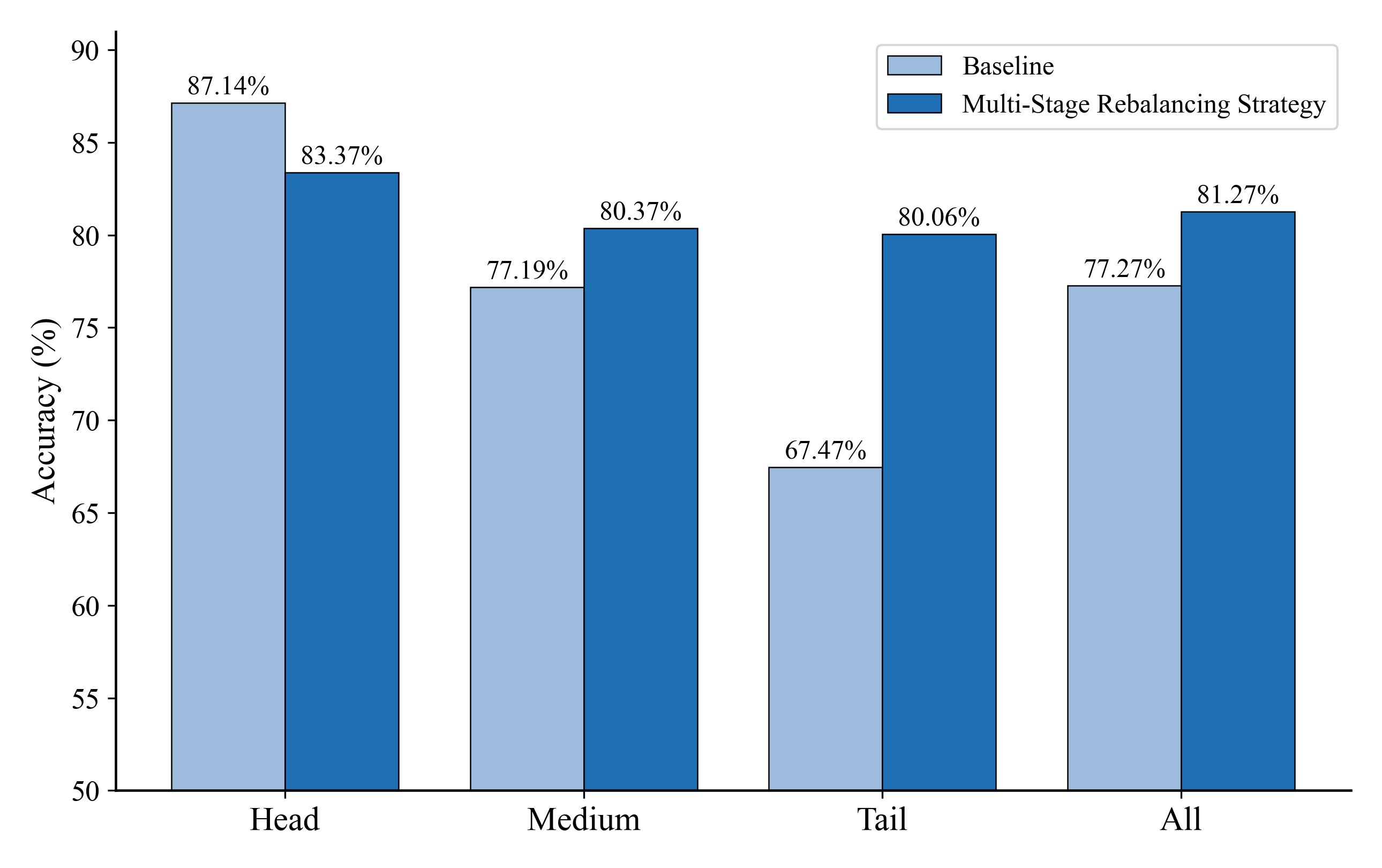
The mean class accuracies are presented in Figure 9, where the baseline model refers to the original ResNet-50 without any adjustments introduced by our method. As shown in the figure, the mean accuracy for tail-class minerals improves significantly from 67.47% to 80.06%, while medium-class minerals improve from 77.19% to 80.37%. Although the accuracy for head-class minerals decreases slightly from 87.14% to 83.37%, the overall mean accuracy increases from 77.27% to 81.27%. As stated in Section 3.1, approximately 5% of the images in the test set may have been trained in the training set. Then, for our overall mean accuracy of 81.27%, 5%× (1 − 0.8127) = 0.94% may be inflated. Considering that the baseline model without our multi-stage rebalancing used the same dataset, its accuracy may be inflated by 5% × (1 − 0.7727) = 1.14%, which is even larger than ours. So our method achieves a higher accuracy increase if the dataset has no similar images. This indicates that the proposed multi-stage rebalancing strategy substantially enhances recognition performance for underrepresented tail and medium classes, with only a minor trade-off in head-class accuracy, ultimately improving the overall classification performance.

Figure 9. Mean accuracy of the multi-stage rebalancing method.

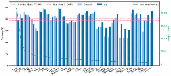
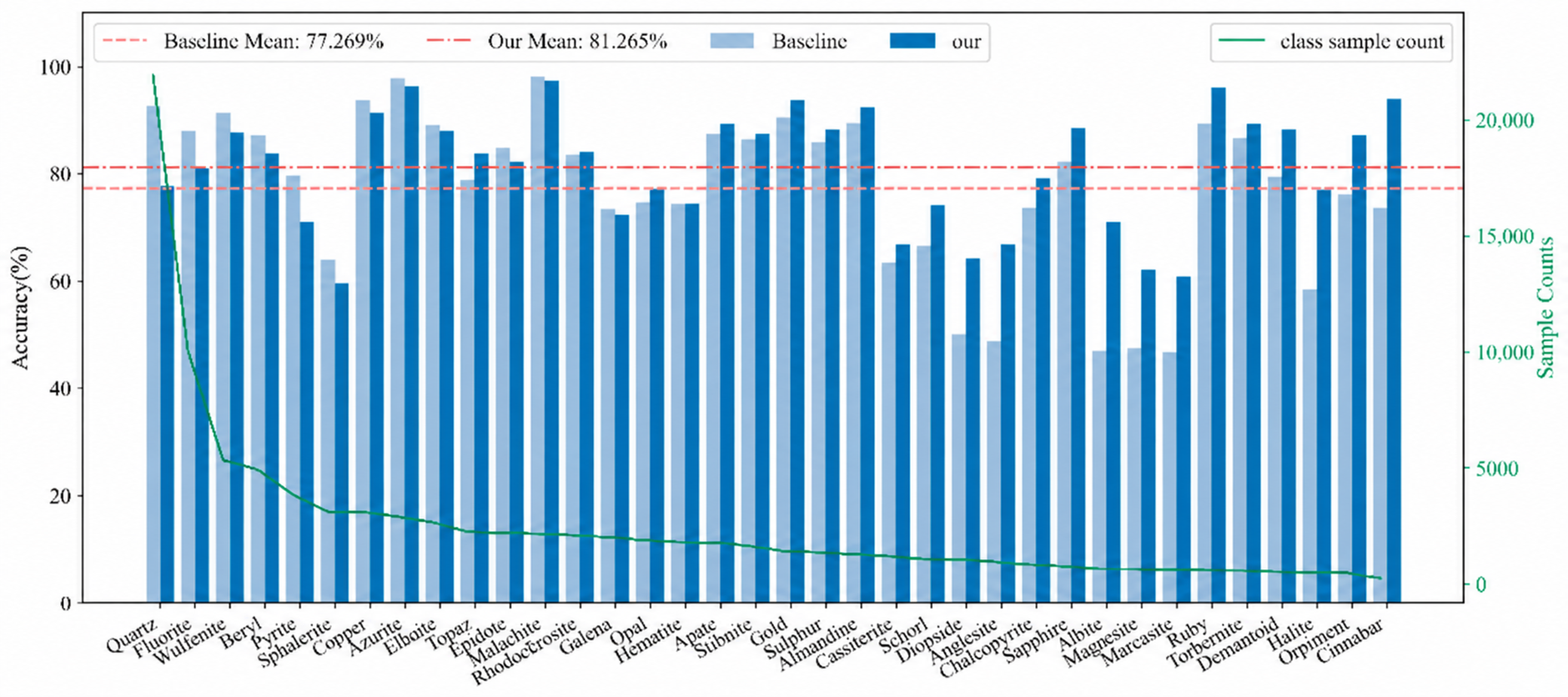
Figure 10 illustrates the per-class accuracy across all mineral categories, showing that the proposed method yields consistent improvements in recognition accuracy for tail-class minerals. Furthermore, as reported in Table 2, the CwASD and CwARange decrease from 0.15 and 0.52 to 0.11 and 0.40, respectively. This further demonstrates the effectiveness of our method in promoting performance balance across classes.

Figure 10. Accuracy of the multi-stage rebalancing method for individual mineral classes.

Table 2. Performance at each stage.

	Many	Medium	Few	All	CwASD	CwARange
Baseline	87.14	77.19	67.47	77.27	0.150	0.513
FEB	85.81	78.87	74.53	79.74	0.126	0.439
CFL	87.06	78.35	68.98	78.13	0.143	0.504
cRT	85.61	78.39	73.62	79.21	0.122	0.453
Multi-Stage	83.37	80.37	80.06	81.27	0.107	0.378

The bold in the table means the best.

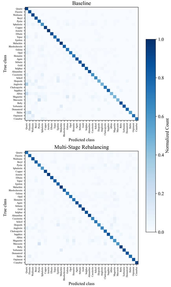
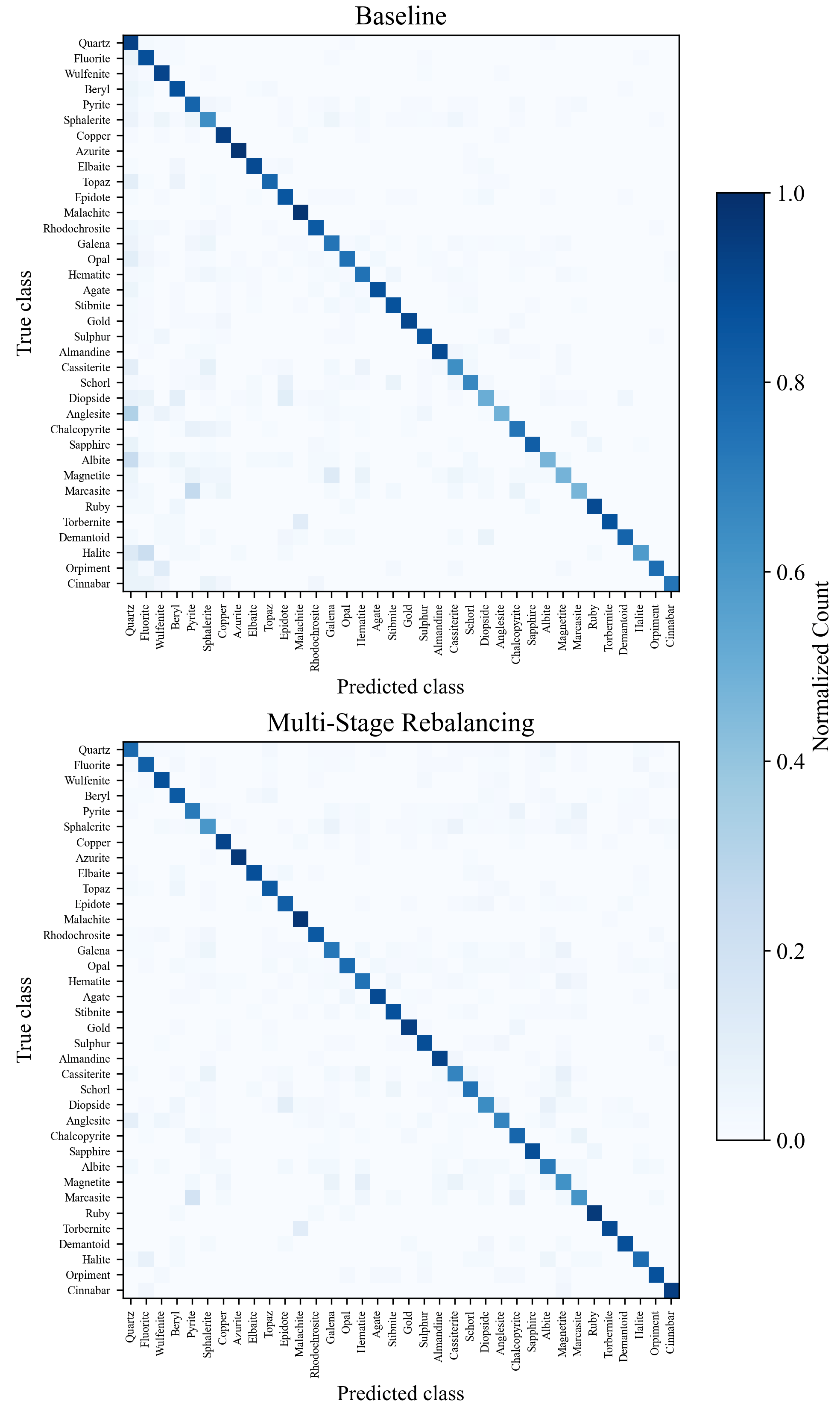
The confusion matrices are visualized in Figure 11. In the baseline model, the lower-left region of the confusion matrix exhibits darker color blocks, indicating a strong bias toward misclassifying tail-class minerals as head-class minerals. After applying the multi-stage rebalancing strategy, the same region becomes noticeably lighter, suggesting that the model’s confusion regarding tail-class minerals has been significantly alleviated. This reflects a more balanced and comprehensive recognition performance in long-tailed mineral classification.

Figure 11. Confusion matrices before and after multi-stage rebalancing, with class labels sorted in descending order of sample size.

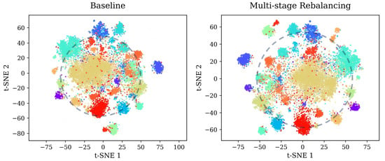
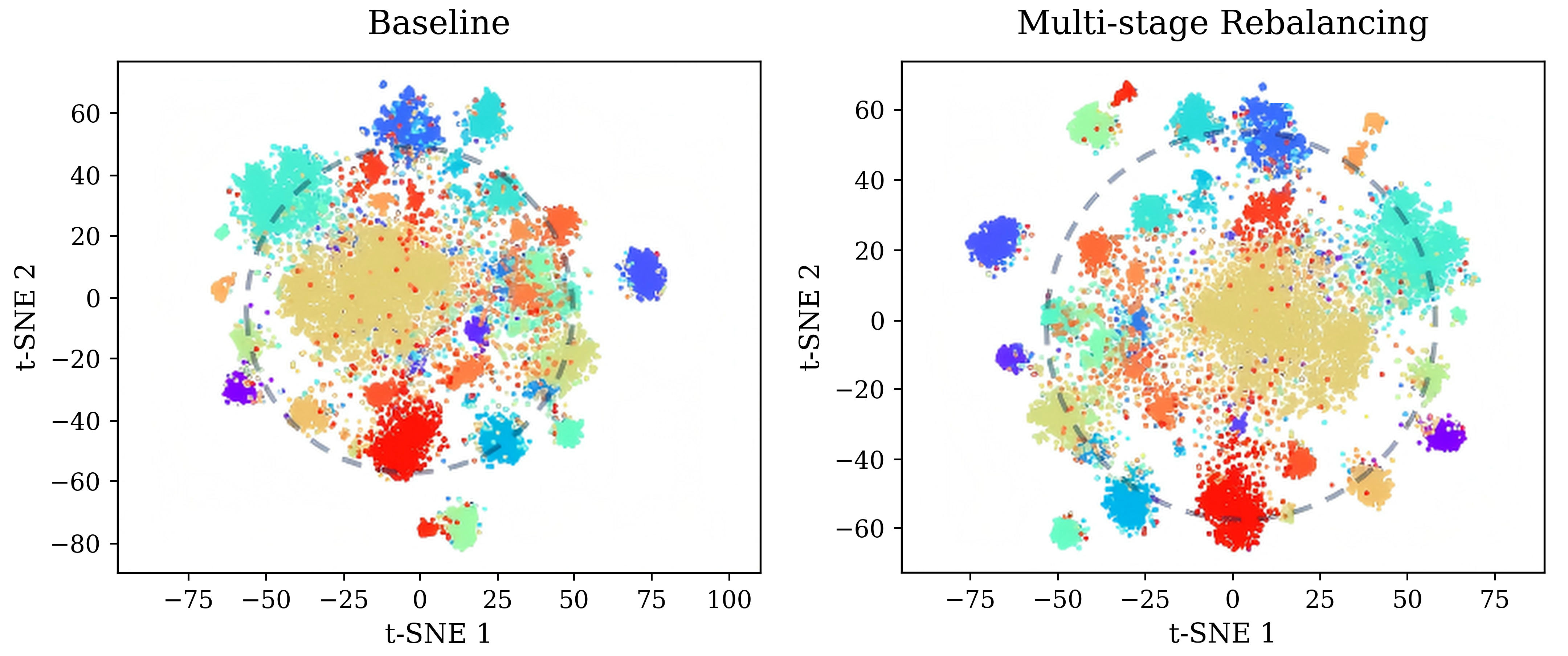
Finally, the two-dimensional visualization of the feature distribution of the 36 categories of minerals on the test set is shown in Figure 12. In Figure 12, different colors represent different categories of minerals, and we can see that after applying the proposed method, the different categories of the minerals are separated more clearly, indicating more effective classification.

Figure 12. Two-dimensional visualizations before and after multi-stage rebalancing.

3.4. Performance Evaluation of Each Balancing Stage

This section provides a detailed evaluation of the effectiveness of each stage within the proposed multi-stage rebalancing strategy, as summarized in Table 2.

3.4.1. Feature Extractor Adjustment

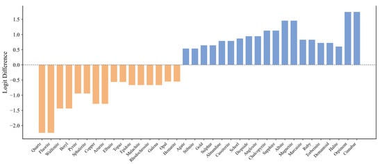
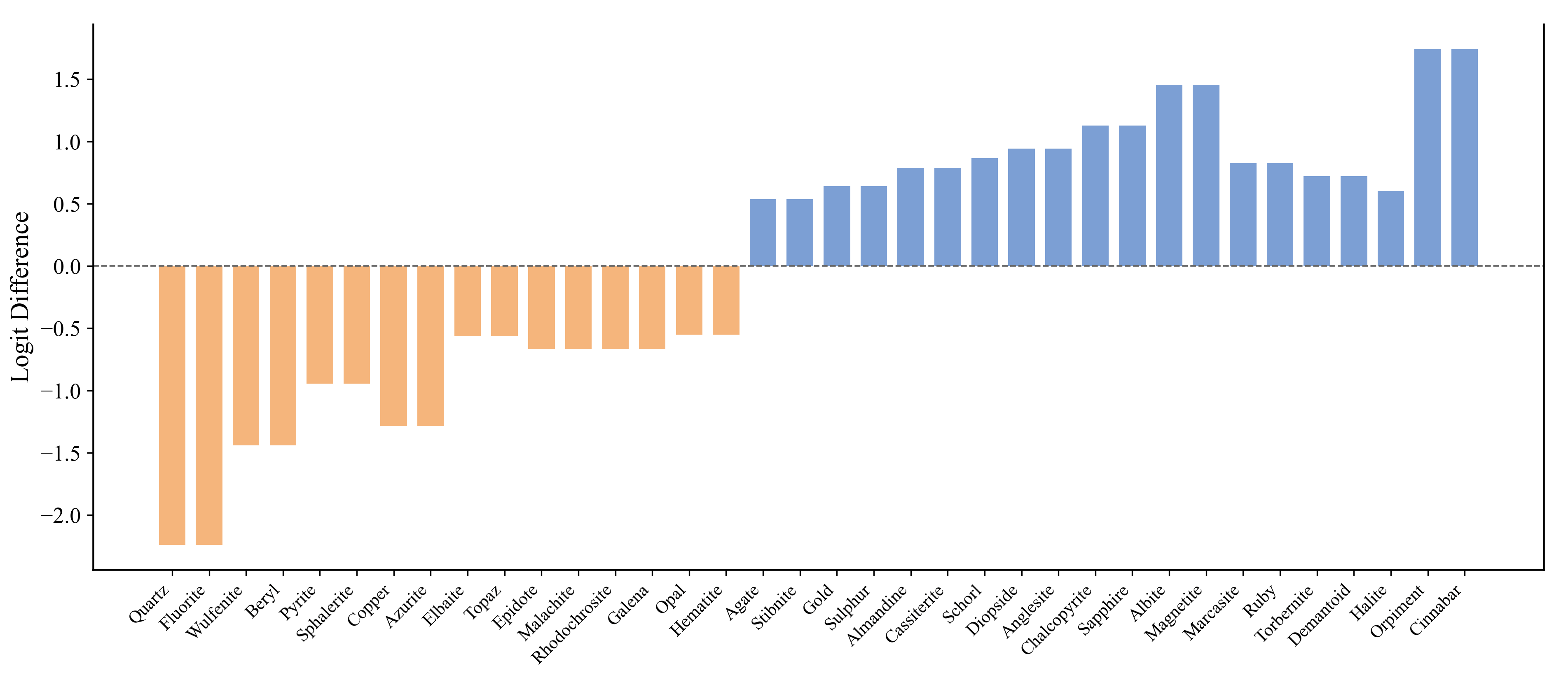
As shown in Table 2, applying feature extractor adjustment significantly improves the mean accuracy for tail-class minerals by 7.06%, while the overall mean accuracy increases by 2.47%. Additionally, the CwASD and CwARange decrease by 0.02 and 0.07, respectively. As illustrated in Figure 13, the visualization of average logit scores before and after adjustment reveals that the logits for tail classes increase substantially, whereas those for head classes slightly decrease, indicating enhanced learning for underrepresented classes. Furthermore, the reduction in CwASD and CwARange suggests that this adjustment helps to narrow the performance gap among different categories. This contributes to improved overall performance and model stability by encouraging more equitable feature representation across classes.

Figure 13. Differences in average logit scores for test samples before and after feature extractor adjustment, sorted in descending order of sample size.

3.4.2. Core Feature Learning

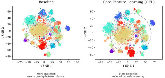
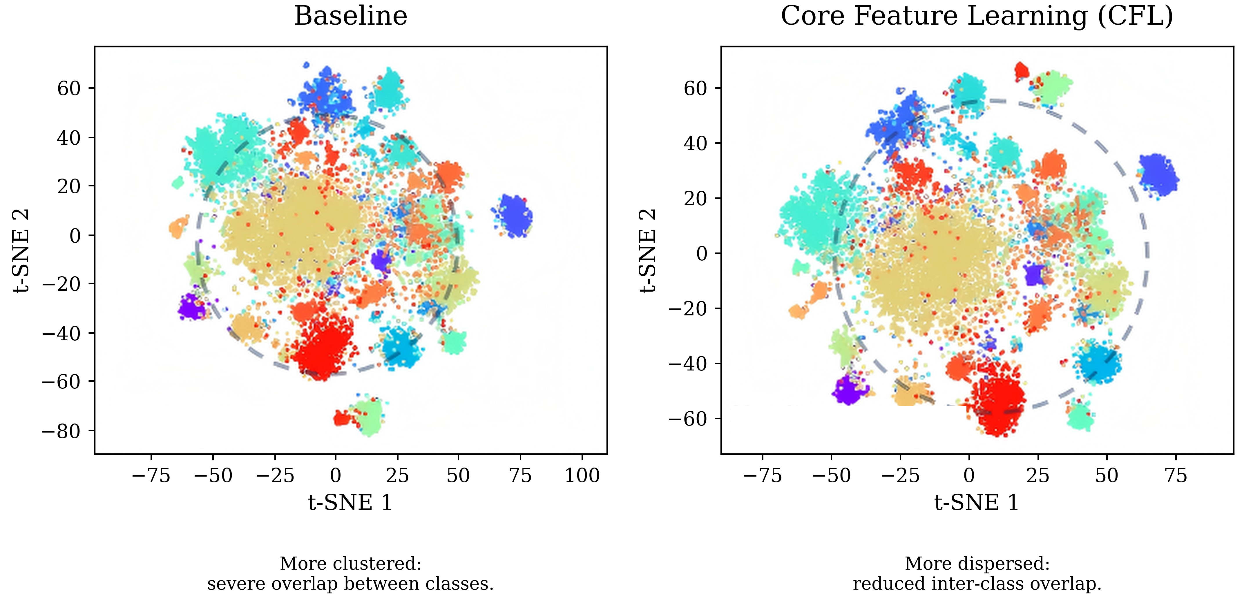
According to Table 2, applying core feature learning alone leads to a 1.16% increase in mean accuracy for medium classes, a 1.51% increase for tail-class minerals, and a 0.86% improvement in overall mean accuracy. The two-dimensional visualizations of feature distributions before and after core feature learning are shown in Figure 14, where different colors represent different categories of minerals, as in Figure 12, and after applying core feature learning, the different categories of minerals are separated more clearly, and the overlap among different classes is substantially reduced.

Figure 14. Two-dimensional visualization before and after core feature learning.

Moreover, core feature learning minimally affects the performance of head classes, with only a negligible 0.08% drop in head-class mineral accuracy. This highlights its strong ability to perceive and adapt to intra-class diversity, contributing to a more comprehensive improvement in recognition performance without significantly sacrificing the accuracy of dominant classes.

3.4.3. Classifier Re-Training

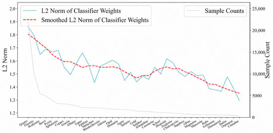
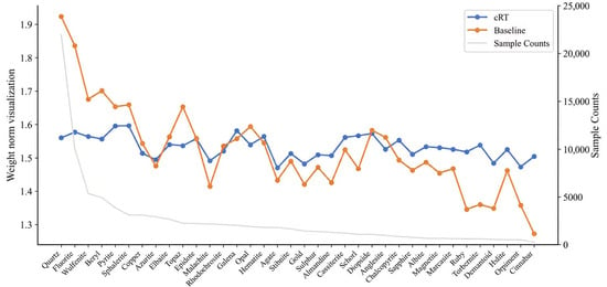
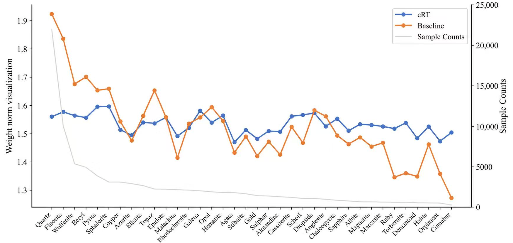
As shown in Table 2, applying classifier re-training alone results in a 6.15% increase in mean accuracy for tail-class minerals, along with a 1.94% improvement in overall mean accuracy. The CwASD and CwARange decrease by 0.03 and 0.06, respectively. Figure 15 presents the L2 norm [31] of weight vectors for each class in the classifier. Compared to the baseline model (orange line), the classifier after re-training (blue line) exhibits a more balanced distribution of weight magnitudes. Specifically, the weights for tail-class minerals are significantly enhanced, while the bias toward head-class minerals is effectively reduced. This indicates that classifier re-training with class-balanced sampling successfully corrects the decision boundaries previously dominated by majority classes. As a result, the model is able to learn a more balanced classifier, leading to significantly improved recognition of tail-class minerals.

Figure 15. L2 norm of classifier weights, sorted in descending order of sample size.

3.5. Ablation Study

To evaluate the effectiveness of each component within the proposed multi-stage balancing framework, three ablation experiments were conducted by selectively removing individual components, as summarized in Table 3.

Table 3. Ablation study.

FEB	CFL	cRT	Many	Medium	Few	All	CwASD	CwARange
-	-	-	87.14	77.19	67.47	77.27	0.150	0.513
√	√	-	85.77	79.43	76.02	80.41	0.121	0.462
√	-	√	82.11	79.69	79.48	80.43	0.110	0.401
-	√	√	86.67	79.16	71.90	79.24	0.123	0.472
√	√	√	83.37	80.37	80.06	81.27	0.107	0.378

The bold in the table means the best, and “√” means the corresponding component is activated in the framework.

Feature extractor adjustment and classifier re-training exhibit a strong synergistic effect in enhancing tail-class performance. Their combination yields a 12.01% increase in the average accuracy of tail-class minerals, a 3.16% improvement in overall mean accuracy, and reductions of 0.04 and 0.11 in CwASD and CwARange, respectively. This represents the most substantial improvement in tail-class recognition among all two-component combinations. However, this enhancement comes at the cost of a 5.03% decrease in head-class accuracy, indicating that while the method effectively narrows performance disparities across classes, it may adversely affect the recognition of majority classes.

The combination of feature extractor adjustment and core feature learning also demonstrates a degree of synergy. While boosting tail-class performance, this combination has a much milder impact on head-class accuracy, suggesting a more balanced trade-off between improving minority-class performance and preserving majority-class performance. In contrast, classifier re-training and core feature learning do not exhibit a strong synergistic effect in improving tail-class performance. This is because both techniques involve class-balanced sampling strategies, particularly for one of the sample subsets used in core feature learning. This overlap in sampling design may reduce their combined impact on tail-class rebalancing. Overall, the model achieves the best balance of performance when all three components—feature extractor adjustment, core feature learning, and classifier re-training—are applied jointly.

4. Discussion

Our experiments in Section 3 did not compare our method with established long-tailed baselines such as LDAM (label-distribution-aware margin), CB (class-balanced) loss, OLTR (Open Long-Tailed Recognition), or decoupled training. The reason is that the logit adjustment formulation we applied has been systematically compared against focal, class-balanced focal, LDAM, and CB Loss, and reports competitive or superior performance to that in reference [26]. So we use logit adjustment here as a representative, theoretically grounded formulation of this family. Regarding OLTR, which is designed for open-set long-tailed recognition, in which, in addition to recognizing the known classes, the model must also detect inputs that belong to none of them (“unknown” images); in our closed-set recognition, by contrast, every test image is assumed to belong to one of the 36 fixed classes and no unknown-class detection is required. So OLTR is not compared.

The specific solutions of the proposed framework are at the loss level, the sampling level, and the classifier level, which are all unrelated to architecture. So the evaluations in this study follow a paired within-architecture design (the same backbone and configuration, with and without the proposed strategy), which isolates the contribution of the training strategy from architecture-specific factors. We agree that empirical validation across additional backbones would further strengthen the generality claim and will be conducted in our future work.

As stated in Section 3.1, the dataset may contain 3529 pairs of images that are possible variants of the same source. The experimental results and the corresponding analysis in Section 3.3 show that our method will obtain an even higher accuracy increase if the dataset has no similar images. Experiments on the dataset removing the similar pairs will be conducted in our next work to provide a more reliable assessment of the actual generalization capability of the proposed method. Mean class accuracy (mAcc), the Class-Wise Accuracy Standard Deviation (CwASD), and the Class-Wise Accuracy Range (CwARange) are the three metrics used to evaluate the method. In the single-label closed-set setting, mAcc is mathematically equivalent to the balanced accuracy, because each class’s accuracy equals that class’s recall and both metrics are the unweighted macro-average of per-class scores. Other metrics like macro-F1 will be tested in our future work.

Two-dimensional visualizations, as shown in Figure 12 and Figure 14, are used to manifest the effectiveness of our strategies. Because it appears more visually intuitive from the figures, specific numerical values (e.g., inter-class distance or silhouette score) are not provided. The data in this study are partitioned at the image level, which covers 36 common rock-forming, ore, and gem minerals. A dedicated comparison relating relative abundance to per-category recognition performance across mineral types is planned as a future extension.

The feature extraction of the ResNet model we use is automated, like other deep learning models, or in other words, a black box, making it difficult to understand how it arrives at specific decisions. So it is difficult to point out the target features and how those can be linked to the real classifiers to identify minerals. From a practical perspective, the proposed framework operates on macroscopic hand-specimen photographs and provides a fast, automatic aid for the macroscopic first-glance screening of mineral hand specimens before confirmation by professional means.

The contribution of this paper lies in putting forward the issue of data imbalance in macroscopic hand-specimen photograph identification based on deep learning and proposing corresponding solutions. The data used in this paper are from an existing database, not a specific location. Evaluating the method on data from specific locations will be our next work, and we look forward to combining the method with the borehole sections, geological sections, geophysical/geochemistry observations, and satellite/remote-sensing data for quick and accurate mineral exploration in the future. Intense communication and close cooperation with geoscientists will be conducted further, as suggested in reference [43].

5. Conclusions

To address the issue of data imbalance in mineral image recognition, this study proposes a multi-stage rebalancing strategy that significantly enhances the overall performance of mineral recognition models. It addresses three distinct and complementary sources of imbalance in mineral image recognition. Feature extractor adjustment handles the frequency imbalance across classes by re-weighting the loss according to class frequency; core feature learning handles intra-class attribute imbalance by re-weighting the sampling toward low-confidence instances and enforcing class-center consistency; and classifier re-training corrects the residual decision-boundary bias that favors majority classes. The ablation study confirms this complementarity: the strongest two-component combination (feature extractor adjustment with classifier re-training) improves the mean tail accuracy by 12.01%, and adding core feature learning further improves the tail and overall accuracy with a mild effect on head classes, yielding the best overall balance. By integrating feature extractor adjustment, core feature learning, and classifier re-training, the proposed method improves the average recognition accuracy of the bottom one-third (tail classes) on a 36-category mineral dataset from 67.47% to 80.06%, with a maximum improvement of 24.1%. Meanwhile, the overall average recognition accuracy increases from 77.27% to 81.27%, demonstrating the effectiveness of the proposed strategy in mitigating long-tail recognition challenges in mineral classification tasks.

Empirical validation across additional backbones, more metrics, and data from specific locations will be conducted in the future. Intense communication and close cooperation with geoscientists will be strengthened, and the combination of the method with borehole sections, geological sections, geophysical/geochemistry observations, and satellite/remote-sensing data for quick and accurate mineral exploration is expected.

References

- Eppelbaum, L.; Eppelbaum, V.; Ben-avraham, Z. Formalization and estimation of integrated geological investigations: An informational approach. Geoinformatics 2003, 14, 233–240. [Google Scholar] [CrossRef] [Scilit]
- Yang, F.; Zuo, R.; Kreuzer, O.P. Artificial intelligence for mineral exploration: A review and perspectives on future directions from data science. Earth-Sci. Rev. 2024, 258, 104941. [Google Scholar] [CrossRef] [Scilit]
- Yang, H.; Feng, W.; Diao, H.; Xia, S. Artificial intelligence transforming minerals engineering: Key trends in literature and applications. Miner. Eng. 2025, 234, 109741. [Google Scholar] [CrossRef] [Scilit]
- Lee, S.; Moon, I. Recent Advances and Future Perspectives of AI-Based Mineral Exploration: A Review of Machine Learning, Deep Learning, and Geologically Informed Approaches. Minerals 2026, 16, 584. [Google Scholar] [CrossRef] [Scilit]
- Lou, W.; Zhang, D.; Bayless, R.C. Review of mineral recognition and its future. Appl. Geochem. 2020, 122, 104727. [Google Scholar] [CrossRef] [Scilit]
- Liu, Y.; Wang, X.; Zhang, Z.; Deng, F. A review of deep learning in image classification for mineral exploration. Miner. Eng. 2023, 204, 108433. [Google Scholar] [CrossRef] [Scilit]
- Peng, W.; Bai, L.; Shang, S.; Tang, X.; Zhang, Z. Common mineral intelligent recognition based on improved InceptionV3. Geol. Bull. China 2019, 38, 2059–2066. (In Chinese) [Google Scholar]
- Li, M.; Liu, C.; Zhang, Y.; Zhu, Y.Q. A Deep learning and intelligent recognition method of Image data for rock mineral and its implementation. Geotecton. Metallog. 2020, 44, 203–211. (In Chinese) [Google Scholar]
- Brempong, E.A.; Agangiba, M.; Aikins, D. MiNet: A convolutional neural network for identifying and categorising minerals. Ghana J. Technol. 2020, 5, 86–92. [Google Scholar]
- Theerthagiri, P.; Ruby, A.U.; Chandran, J.G.C. Prediction and classification of minerals using a deep residual neural network. Neural Comput. Appl. 2024, 36, 1539–1551. [Google Scholar] [CrossRef] [Scilit]
- Li, L.; Lu, C.; Jiang, S.; Jing, W.; Wang, L. Intelligent recognition of mineral images based on an improved ConvNeXt network. Geol. Bull. China 2024, 43, 1266–1275. (In Chinese) [Google Scholar]
- Jia, L.; Chen, F.; Yang, M.; Meng, F.; He, M.; Liu, H. SwinMin: A mineral recognition model incorporating convolution and multi-scale contexts into swin transformer. Comput. Geosci. 2024, 184, 105532. [Google Scholar] [CrossRef] [Scilit]
- He, L.; Zhou, Y.; Zhang, C. Application of target detection based on deep learning in intelligent mineral identification. Minerals 2024, 14, 873. [Google Scholar] [CrossRef] [Scilit]
- Zeng, X.; Xiao, Y.; Ji, X.; Wang, G. Mineral identification based on deep learning that combines image and Mohs hardness. Minerals 2021, 11, 506. [Google Scholar] [CrossRef] [Scilit]
- Liao, H.; Ji, X.; Yang, M.; He, M.; Lv, G.; Liu, M.; Zhang, Z.; Zeng, S.; Li, J.; Wang, Y. Mineral identification based on multimodal and knowledge distillation. Nat. Resour. Res. 2026, 35, 679–695. [Google Scholar] [CrossRef] [Scilit]
- Liao, H.; Ji, X.; Yang, M.; Xu, B.; Lv, G.; Liu, M.; Li, J. Robust multimodal mineral identification based on a parameter-efficient method. Comput. Geosci. 2026, 215, 106228. [Google Scholar] [CrossRef] [Scilit]
- Le Quy, T.; Roy, A.; Iosifidis, V.; Zhang, W.; Ntoutsi, E. A survey on datasets for fairness-aware machine learning. WIREs Data Min. Knowl. Discov. 2022, 12, e1452. [Google Scholar] [CrossRef] [Scilit]
- Yang, L.; Jiang, H.; Song, Q.; Guo, J. A survey on long-tailed visual recognition. Int. J. Comput. Vis. 2022, 130, 1837–1872. [Google Scholar] [CrossRef] [Scilit]
- Zhang, Y.; Kang, B.; Hooi, B.; Yan, S.; Feng, J. Deep long-tailed learning: A survey. IEEE Trans. Pattern Anal. Mach. Intell. 2023, 45, 10795–10816. [Google Scholar] [CrossRef] [Scilit] [PubMed]
- Fu, Y.; Xiang, L.; Zahid, Y.; Ding, G.; Mei, T.; Shen, Q.; Han, J. Long-tailed visual recognition with deep models: A methodological survey and evaluation. Neurocomputing 2022, 509, 290–309. [Google Scholar] [CrossRef] [Scilit]
- Nesteruk, S.; Agafonova, J.; Pavlov, I.; Gerasimov, M.; Latyshev, N.; Dimitrov, D.; Kuznetsov, A.; Kadurin, A.; Plechov, P. MineralImage5k: A benchmark for zero-shot raw mineral visual recognition and description. Comput. Geosci. 2023, 178, 105414. [Google Scholar] [CrossRef] [Scilit]
- Yu, H.; Du, Y.; Wu, J. Reviving undersampling for long-tailed learning. arXiv 2024, arXiv:2401.16811. [Google Scholar]
- Li, M.; Hu, Z.; Lu, Y.; Lan, W.; Cheung, Y.-M.; Huang, H. Feature fusion from head to tail for long-tailed visual recognition. Proc. AAAI Conf. Artif. Intell. 2024, 38, 13581–13589. [Google Scholar] [CrossRef] [Scilit]
- Zhao, S.; Wen, X.; Liu, J.; Ma, C.; Yuan, C.; Qi, X. Learning from neighbors: Category extrapolation for long-tail learning. In Proceedings of the IEEE/CVF Conference on Computer Vision and Pattern Recognition (CVPR), Nashville, TN, USA, 10–17 June 2025; pp. 30483–30492. [Google Scholar] [CrossRef] [Scilit]
- Zhao, Z.; Wang, H.; Shang, Y.; Wang, K.; Yan, Y. Distilling long-tailed datasets. In Proceedings of the IEEE/CVF Conference on Computer Vision and Pattern Recognition (CVPR), Nashville, TN, USA, 10–17 June 2025; pp. 30609–30618. [Google Scholar] [CrossRef] [Scilit]
- Yang, J.; Zhang, R.; Shang, C.; Li, M.; Shang, X.; Gao, J.; Zhang, Y.; Lu, Y. Decision boundary-aware generation for long-tailed learning. In Proceedings of the IEEE/CVF Conference on Computer Vision and Pattern Recognition (CVPR), Denver, CO, USA, 3–7 June 2026; pp. 29441–29450. [Google Scholar]
- Menon, A.K.; Jayasumana, S.; Rawat, A.S.; Jain, H.; Veit, A.; Kumar, S. Long-tail learning via logit adjustment. In Proceedings of the International Conference on Learning Representations (ICLR), Virtual, 3–7 May 2021. [Google Scholar]
- Laurent, T.; Brecht, J.H.; Bresson, X. Long-tailed learning requires feature learning. arXiv 2022, arXiv:2205.14553. [Google Scholar]
- Tang, K.; Tao, M.; Qi, J.; Liu, Z.; Zhang, H. Invariant feature learning for generalized long-tailed classification. In Computer Vision—ECCV 2022; Springer: Cham, Switzerland, 2022; Volume 13684, pp. 709–726. [Google Scholar] [CrossRef] [Scilit]
- Yang, J.; Xu, J.; Wu, D.; Tang, J.; Li, S.; Wang, G. Long-tailed classification based on coarse-grained leading forest and multi-center loss. arXiv 2023, arXiv:2310.08206. [Google Scholar]
- Kang, B.; Xie, S.; Rohrbach, M.; Yan, Z.; Gordo, A.; Feng, J.; Kalantidis, Y. Decoupling representation and classifier for long-tailed recognition. In Proceedings of the International Conference on Learning Representations (ICLR), Virtual, 26 April–1 May 2020. [Google Scholar]
- Liu, W.; Wen, Y.; Yu, Z.; Yang, M. Large-margin softmax loss for convolutional neural networks. In Proceedings of the 33rd International Conference on Machine Learning, New York, NY, USA, 20–22 June 2016; Volume 48, pp. 507–516. [Google Scholar]
- Kang, B.; Li, Y.; Xie, S.; Yuan, Z.; Feng, J. Exploring balanced feature spaces for representation learning. In Proceedings of the International Conference on Learning Representations (ICLR), Virtual, 3–7 May 2021. [Google Scholar]
- Tao, Y.; Sun, J.; Yang, H.; Chen, L.; Wang, X.; Yang, W.; Du, D.; Zheng, M. Local and global logit adjustments for long-tailed learning. In Proceedings of the IEEE/CVF International Conference on Computer Vision (ICCV), Paris, France, 1–6 October 2023; pp. 11783–11792. [Google Scholar] [CrossRef] [Scilit]
- Zhong, Z.; Cui, J.; Liu, S.; Jia, J. Improving calibration for long-tailed recognition. In Proceedings of the IEEE/CVF Conference on Computer Vision and Pattern Recognition (CVPR), Virtual, 19–25 June 2021; pp. 16489–16498. [Google Scholar] [CrossRef] [Scilit]
- Wen, Y.; Zhang, K.; Li, Z.; Qiao, Y. A discriminative feature learning approach for deep face recognition. In Computer Vision—ECCV 2016; Springer: Cham, Switzerland, 2016; Volume 9911, pp. 499–515. [Google Scholar] [CrossRef] [Scilit]
- Arjovsky, M.; Bottou, L.; Gulrajani, I.; Lopez-Paz, D. Invariant risk minimization. arXiv 2019, arXiv:1907.02893. [Google Scholar]
- Cong, C.; Xuan, S.; Liu, S.; Zhang, S.; Pagnucco, M.; Song, Y. Decoupled optimisation for long-tailed visual recognition. Proc. AAAI Conf. Artif. Intell. 2024, 38, 1380–1388. [Google Scholar] [CrossRef] [Scilit]
- Xuan, S.; Zhang, S. Decoupled contrastive learning for long-tailed recognition. Proc. AAAI Conf. Artif. Intell. 2024, 38, 6396–6403. [Google Scholar] [CrossRef] [Scilit]
- Tarawneh, A.S.; Hassanat, A.B.; Altarawneh, G.A.; Almuhaimeed, A. Stop oversampling for class imbalance learning: A review. IEEE Access 2022, 10, 47643–47660. [Google Scholar] [CrossRef] [Scilit]
- Zauner, C. Implementation and Benchmarking of Perceptual Image Hash Functions. Master’s Thesis, Upper Austria University of Applied Sciences, Hagenberg, Austria, 2010. [Google Scholar]
- Samanta, P.; Jain, S. Analysis of Perceptual Hashing Algorithms in Image Manipulation Detection. Procedia Comput. Sci. 2021, 185, 203–212. [Google Scholar] [CrossRef] [Scilit]
- Stöllner, T. What is an Ore Deposit? Approaches from Geoscience and Archaeology in Understanding the Usage of Deposits. Metalla 2019, 24, 87–110. [Google Scholar] [CrossRef] [Scilit]
Disclaimer/Publisher’s Note: The statements, opinions and data contained in all publications are solely those of the individual author(s) and contributor(s) and not of MDPI and/or the editor(s). MDPI and/or the editor(s) disclaim responsibility for any injury to people or property resulting from any ideas, methods, instructions or products referred to in the content. |
© 2026 by the authors. Licensee MDPI, Basel, Switzerland. This article is an open access article distributed under the terms and conditions of the Creative Commons Attribution (CC BY) license.