


Abstract
Energy piles are multifunctional deep foundations that structurally support buildings while enabling heat exchange between the superstructure and shallow subsurface. It is crucial for the wider use of energy piles and thus reliance on clean, renewable shallow geothermal energy for supplemental space heating and cooling to understand thermal and combined thermo-mechanical load transfer. To this end, previously developed and successfully validated analytical solutions are transformed into a unified dimensionless form, and the minimum set of controlling composite parameters is identified through rigorous application of the Buckingham Π theorem. A multifaceted solution space is explored through a sensitivity analysis performed across a wide range of controlling parameters and under different boundary conditions. The results show that the mechanisms of load transfer for thermal and mechanical loads are inherently different. In a very stiff soil, mechanical load is supported by the soil, while thermal load generates significant stress in the pile. Thus, the thermo-mechanical stress response is dominated by the thermal response. In a very soft soil, mechanical load is supported by the pile while stresses generated by thermal load are negligible. Thus, the thermo-mechanical stress response is dominated by the mechanical response.
1. Introduction
Energy piles are multifunctional deep foundations that facilitate heat exchange between the shallow subsurface and the superstructure, in addition to providing the structural support for the buildings. A plastic tube is inserted into these piles to provide a conduit for the heat-exchange fluid circulated by the ground-source heat pump. Energy piles withdraw the heat stored in the shallow subsurface during winter and release heat into the ground during summer, thus facilitating supplemental or total space heating and cooling. Furthermore, energy piles enable the use of clean, renewable shallow geothermal energy and decrease reliance on fossil fuels.
Different approaches, including physical, numerical, and analytical modeling, have been used in the past to advance our understanding of thermal and thermo-mechanical load transfer in energy piles, which is crucial for the wider use of energy piles, increased sustainability of civil infrastructure, and decreased reliance on fossil fuels. However, physical and numerical models are inherently limited in number, whereas analytical solutions, once successfully validated, are virtually limitless, enabling the exploration of a wide spectrum of responses.
There is currently only a very limited number of analytical solutions for thermo-mechanical displacement, strain, and stress in single-energy piles available in the literature. Cossel [1] derived analytical solutions for a single energy pile embedded in a four-layered soil. Iodice et al. [2] provided analytical solutions for a single energy pile embedded in a two-layered soil and in a soil with linearly increasing stiffness with depth. Perić et al. [3] and Saeidi et al. [4] provided analytical solutions for a single end-bearing and semi-floating energy pile, respectively. Olia and Perić [5] and Saeidi and Perić [6] derived analytical solutions for a single energy pile embedded in a homogeneous soil and subjected to different boundary conditions, with reversible and irreversible soil-pile interfaces, respectively.
This study focuses on the analytical approach. To this end, previously developed and successfully validated analytical solutions are formulated in an elegant dimensionless form. The novel feature is the use of the Buckingham Π theorem to identify the minimum number of controlling composite parameters. Furthermore, a combined dimensionless thermo-mechanical solution is introduced, which enables the consideration of varying thermal loads under a constant mechanical load. The multifaceted dimensionless displacement and stress space is subsequently explored by generating the response spectrum of a single energy pile subjected to constant mechanical and varying thermal loads over a wide range of controlling parameters and different boundary conditions. This approach advanced the understanding of the behavioral patterns of energy piles subjected to thermo-mechanical loads. Furthermore, the practical application of dimensionless solutions is demonstrated through a hypothetical design situation.
2. Materials and Methods
2.1. Unified Solution for Thermo-Mechanical Load
An analytical approach is adopted herein, in which a modified derivation of the previously obtained separate solutions for thermal and mechanical loads [4] yields a unified thermo-mechanical solution applicable to different boundary conditions. The analytical solutions were successfully validated against geotechnical centrifuge tests on end-bearing and nearly fully floating energy piles in [5]. Furthermore, the extension of analytical solutions to a semi-floating pile embedded in a multilayered system, presented in [4], was successfully validated against field test data.
The novel approach adopted herein enabled the solution to be normalized into a dimensionless form containing the minimum number of parameters by applying the Buckingham Π theorem [7]. This resulted in an elegant form of solutions for thermo-mechanical displacement, strain, and stress. Additionally, the introduction of an equivalent thermal load enabled the combination of a constant mechanical load with varying thermal loads.
As shown in [5], the governing equation for thermal or mechanical response of an energy pile subjected to the axial force F applied at the pile head or the temperature change ΔT with respect to the surrounding soil is obtained by enforcing vertical equilibrium to an infinitesimal section of the pile, invoking a kinematic relationship, thermo-elastic constitutive relationship for the pile, and linear elastic stress-displacement relationship along the pile shaft and pile tip. Due to the assumed elastic nature of the stress-strain and stress-displacement relationships, thermo-mechanical loads are combined, thus resulting in
for a homogeneous soil. Thus, u = u(x) is the vertical thermo-mechanical displacement of the pile, while the parameter ψ is given by
and ks (kN/m3) is the stiffness of the shear spring attached to the pile shaft, E is the elastic modulus of the pile, while p and A are the perimeter and cross-sectional area of the pile, respectively. Ratio of shear spring stiffness and pile’s modulus of elasticity is denoted by ξ, and D is either the pile diameter or the length of the side for circular or square cross section, respectively. Both x and u are positive upwards; compressive force, stress, and strain are all negative, while ΔT is positive for heating. Additional assumptions in [5] include the one-dimensional nature of the problem, uniform temperature change along the x-axis, and independence of material properties from the temperature change.
The general solution of Equation (1) is given by:
The solution for thermo-mechanical strain (ε) is obtained by invoking the kinematic relationship, thus resulting in
and the solution for thermo-mechanical stress is obtained based on the thermo-elastic response of the energy pile as:
where εσ is stress-inducing strain, and εf is free strain, while α is the thermal expansion coefficient of the pile. Equation (5) covers mechanical loading (r = 0) and thermal loading (r = 1).
Constants C1 and C2 are determined from the following boundary conditions:
and
where L is pile length, s = 1 for mechanical loading and s = 0 for thermal loading, and for the combined thermo-mechanical load, r = s = 1. It is noted that only compressive forces are applied at the pile head in this study. Combining Equations (3) and (5) through (7) results in
The combination of Equations (4) and (8) results in
Equation (8) combined with Equation (5) results in
Equations (8)–(10) provide solutions for a semi-floating pile where ξb = kb/E is the ratio of normal spring stiffness at the pile tip and the pile’s elastic modulus.
Solutions for displacement and stress in the end-bearing pile can be obtained from Equations (8) and (10) by letting , resulting in
and
Solutions for a fully floating pile are obtained from Equations (8) and (10) by letting , resulting in
and
2.2. Dimensional Analysis Using the Buckingham Π Theorem
The dimensionless form of the analytical solutions was obtained via dimensional analysis using the Buckingham Π theorem [7,8,9]. The theorem is valid for any physically meaningful, dimensionally homogeneous equation, thus enabling all physical variables to be expressed in terms of a set of independent fundamental dimensions. The theorem states that a physical relationship among variables, whose dimensional matrix has rank , can be expressed in terms of independent dimensionless (Π) groups [9,10]:
The analysis was carried out in the mass–length–time–temperature (–––) system of fundamental dimensions, separately for thermal and mechanical loadings. The dimensions of all variables, the dimensional matrices, and the step-by-step derivation of each Π group are provided in Appendix A.
2.2.1. Governing Variables
The solutions for u and σ provided in Equations (8)–(10) are additively decomposed into thermal (uT εT, σT), and mechanical (uM, εM, σM) parts. The displacement at the location along the pile, under thermal and mechanical loading, depends on the following variables:
so that the number of variables is for thermal loading and for mechanical loading, respectively. The cross-sectional area and perimeter are not independent variables, because they are determined by and the shape of the piles’ cross-section ( and ). The strain and the stress depend on the same independent variables as the displacement, as given in Equation (16).
2.2.2. Rank of the Dimensional Matrix and Number of Π Groups
2.2.3. Repeating Variables and Π Groups
, , and were selected as repeating variables for thermal loading, and and for mechanical loading. Following the method of repeating variables [10,11], each Π group was formed by combining one of the remaining variables , with the repeating variables as follows
where for mechanical loading, and the exponents , and were obtained by requiring each to be dimensionless (Appendix A.2 and Appendix A.3). The Π groups for the strain and stress were obtained by replacing with and , respectively, which only affects the choice of ., i.e., , , or . The resulting Π groups are listed in the fourth and fifth columns of Table 1, along with the remaining variables () associated with each Π group.
Table 1.
Π groups obtained from the Buckingham Π theorem.
2.2.4. Functional Relationships and Normalized Solutions
According to the Π theorem, each dependent Π group is a function of the remaining groups, for example, . Two rules were used to obtain the normalized solutions: (1) any product or power of Π groups is also a Π group [8,9]; and (2) because the pile behavior is thermo-elastic, the interface springs are linear and the load ( or ) is the only source term; all solutions are proportional to , which can therefore be removed from the arguments of the function . Results in Table 1 indicate that Π2 is the dimensionless x coordinate, xN, given by:
Dividing the dependent Π groups by , and using results in the normalized thermal and mechanical displacement, strain, and stress as:
Denoting , with previously defined and , the stiffness groups (Π4 and Π5) become and (Appendix A.4), so that for both thermal and mechanical loading
2.2.5. Composite Groups
For circular and square piles (), the composite parameter and the tip stiffness group are products of powers of the Π groups in Table 1:
2.2.6. Minimal Set of Dimensionless Groups
The Π theorem gives three independent groups in addition to , which are (, and ). The number of groups is further reduced by expressing the governing equation (Equation (1)) in terms of and , resulting in
The dimensionless boundary value problem contains only and , i.e., and affect the normalized response through , and affects only through . This reduction of the Π groups using the governing equation is known as inspectional analysis [12,13]. Therefore,
None of these groups can be removed: is the location at which the response is evaluated, the response changes with (e.g., the maximum normalized thermal displacement of the end-bearing pile, ), and it changes with at a fixed . In the limiting cases of the end-bearing pile () and the fully floating pile (), the response depends on and only. Hence, all normalized solutions can be expressed in terms of for end-bearing and fully floating piles and for semi-floating piles, and these groups form the minimal set of dimensionless groups governing the problem.
2.3. Equivalent Thermal Load
Normalized displacement from Equation (24) is given by
where the mechanical and thermal displacements are normalized by different quantities. In engineering practice, mechanical load is approximately constant while thermal load varies seasonally and even daily. Thus, it is desirable to express thermal load in terms of mechanical load and normalize the overall displacement (u) with respect to and the overall stress with respect to . To this end, the equivalent temperature change ΔTeq is defined as the temperature change that produces zero overall displacement at the pile head, i.e., the magnitude of the mechanical displacement equals the magnitude of the thermal displacement due to heating at the pile head. Hence, the expression for ΔTeq is obtained by setting the overall displacement at the pile head from Equation (8) equal to zero and combining the resulting equation with Equations (2) and (23), giving
where
for the general case of a semi-floating pile. Values of Iβ for special cases of fully floating and end-bearing piles can be obtained by letting and , respectively, and any temperature change can be expressed as:
where for heating, and for cooling.
Thus, the normalized combined thermo-mechanical displacement can be obtained by using Equations (20), (21), and (29) as:
and the normalized combined thermo-mechanical stress can be obtained by using Equations (20), (21), and (29) as:
2.4. Normalized Dimensionless Thermo-Mechanical Response
Normalized mechanical displacement (), is obtained by combining Equation (8), for r = 0 and s = 1, with Equations (21) and (23), resulting in
Normalized thermal displacement (), is obtained by combining Equation (8), for r = 1 and s = 0, with Equations (20) and (23), resulting in
and at and above the null point, and below the null point.
For end-bearing pile ( Equations (32) and (33) result in:
For a fully floating pile ( Equations (32) and (33) result in:
and
Equation (36) indicates that the thermal null point is located at the mid-length of the fully floating pile ( = 0.5), thus resulting in the thermal displacement having a different sign above the null point and below the null point. Similarly, in the case of a semi-floating pile, the normalized thermal displacement will be positive above the thermal null point and negative below the thermal null point. In this case, according to Equation (33), the thermal null point will be located within the bottom half of the pile length. Normalized mechanical stress (, is obtained by combining Equation (10), for r = 0 and s = 1, with Equations (21) and (23), resulting in
Normalized thermal stress (, is obtained by combining Equation (10) for r = 1 and s = 0 with Equations (20) and (23), resulting in
For end-bearing pile ( Equations (37) and (38) result in:
and
For a fully floating pile ( Equations (37) and (38) result in:
and
3. Results and Discussion
A rigorous mathematical analysis presented in Section 2.2.6 showed that composite parameters that control the normalized dimensionless response of a semi-floating pile are and . From the physics point of view, the controlling parameters can be seen as a composite of geometry and stiffness, specifically length to diameter ratio (η), diameter (D), and ratio of shear spring stiffness and normal spring stiffness at the tip to the pile’s elastic modulus (ξ and ξb). In special cases of end-bearing and fully floating piles, controlling composite parameters reduce to a single parameter . Furthermore, 1/ψ can be viewed as the characteristic load-transfer length over which displacement and axial force decay along the pile, and ψL is the ratio of the pile length to the characteristic length. Additionally, a very small ζ corresponds to a pile that is nearly unrestrained by the soil, and sufficiently large ζ to a pile that is nearly fully restrained.
In this section, the dimensionless form of analytical solutions is used to explore stress and displacement response of energy piles exhibiting different boundary conditions, and subjected to varying thermal load across a wide range of controlling parameters (ξ = 0.01 m−1 and 0.0001 m−1, η = 10 and 40, and D = 1 and 2 m). The definition of indicates that it increases with increasing stiffness ratio (ξ), length to diameter ratio (η), and increasing diameter (D). Finally, two values, ξb (1 m−1 and 0.1 m−1), differing by one order of magnitude, are selected to illustrate the response of semi-floating piles. Table 2 shows the corresponding values of the composite parameter .
The four combinations of these parameters considered in this study yield ζ values of 0.2, 1.1, 2.0, and 11.3, as listed in Table 2. These values of ζ are used to label the curves in the figures presented in Section 3so that each curve can be related to the corresponding combination of ξ, η, and D.
Table 2.
Values of the composite parameter ζ and the corresponding combinations of η, D, and ξ used in Section 3.
3.1. End-Bearing Pile
Dimensionless mechanical and thermal displacements are presented in Figure 1, while Figure 2 and Figure 3 depict dimensionless thermal and mechanical stresses, respectively. These figures indicate that the mechanical stress response is different from the thermal stress response. Specifically, in the case of the smallest stiffness ratio (ξ = 0.0001 m−1) and correspondingly the smallest composite ratio , the normalized mechanical stress magnitude is the largest for mechanical loading (Figure 3), while the magnitude of the normalized thermal stress is the smallest (Figure 2). However, normalized thermal and mechanical displacements are both the largest for .
The stress responses are inherently different because, in the case of mechanical loading, the external force (F) is balanced with both shear stress along the pile shaft and normal stress at the pile tip, while the absence of external load in the case of thermal loading balances the shear stress along the shaft with the normal stress at the pile tip. Thus, the largest shear stiffness and the largest value of generate the largest shear stress and, in turn, the largest axial stress magnitude in the pile in the case of thermal loading. Hence, thermal load is largely supported by the pile. In the case of mechanical loading, the largest value also generates the largest shear stress, and the external load (F) is mostly supported by the soil, not the pile, except for the short length section near the pile head. With decreasing values the magnitude of thermal stress decreases while the magnitude of mechanical stress increases. Displacements, however, exhibit similar expected behavior in thermal and mechanical loading, i.e., the largest value of results in the smallest displacement, while the smallest value of = 0.2 results in the largest displacements in both cases.
Additional insight can be gained by considering the pile to be a rod subjected to heating or cooling. A fully restrained rod would generate axial stress of magnitude accompanied by zero strain corresponding to the magnitude of normalized thermal stress equal to one. A fully unrestrained rod would generate zero stress and an axial strain of magnitude , corresponding to a normalized thermal displacement of one. The maximum magnitude of normalized thermal stress at the pile tip is one for the largest value of , with nearly zero magnitude for the smallest values of . On the other hand, the largest magnitude of normalized displacement at the pile head is nearly one for the smallest value of , with the smallest value of displacement of zero along most of the pile length for the largest value of . Unlike the rod, the pile response is nonuniform vs. length due to shear stress acting along its length. The value of dimensionless mechanical stress at the pile head is one because stress was normalized with
Figure 4 and Figure 5 depict dimensionless displacement and stress, respectively, for combined thermo-mechanical loading, for values of −1 and 1 (panels (Figure 4a,b) and (Figure 5a,b), respectively). implies that, which, by definition (Equation (29)), indicates that the combined displacement at the pile head is zero (Figure 4a). In other words, the amount of heating is such that the corresponding upward positive displacement cancels the mechanically induced downward displacement at the pile head. However, in the case of an end-bearing pile, , and thermal displacement cancels mechanical displacement throughout the pile length, regardless of the value of . Correspondingly, for , the normalized combined stress is constant vs. depth and equal to one regardless of the value (Figure 5a). In the case of cooling by the same magnitude, i.e., , mechanical and thermal displacements add up, thus resulting in the largest displacement for the smallest value of (Figure 4b). However, the combined normalized displacement is now twice as large as either the thermal or the mechanical displacement alone. The magnitude of the normalized combined stress increases with increasing value, as explained previously, resulting in the value of one corresponding to the fully restrained pile at the tip (Figure 5b). It is noted that tensile stresses at the pile tip cannot occur in reality as the end-bearing pile transforms to a fully floating pile at the point when the magnitude of the combined stress at the tip becomes equal to zero.
Figure 6 and Figure 7 show the combined normalized displacement and stress responses for additional selected values representing different thermal-load magnitudes, with the heating response in the top row and the cooling response in the bottom row. The previous observation of a smaller value, resulting in a larger displacement, is confirmed in Figure 6. Furthermore, as expected, the magnitude of heating displacements is smaller than that of cooling displacements for the same χ value, simply because both mechanical and cooling displacements are directed downwards, whereas in the case of heating, thermal displacement is directed upwards. Thus, for the smallest value, the normalized displacements at the pile head for heating and χ = −0.5, −1, and −2 are 0.5, 0, and −1, while for cooling and χ = 0.5, 1, and 2, the corresponding normalized displacements are 1.5, 2, and 3. The normalized stress response depicted in Figure 7 shows that the combined response is governed by the mechanical response at the smallest thermal load magnitude, i.e., the largest normalized stress magnitude occurs for the lowest value of . On the contrary, the combined normalized stresses are the largest for the largest value of for the largest magnitude of thermal load, i.e., .
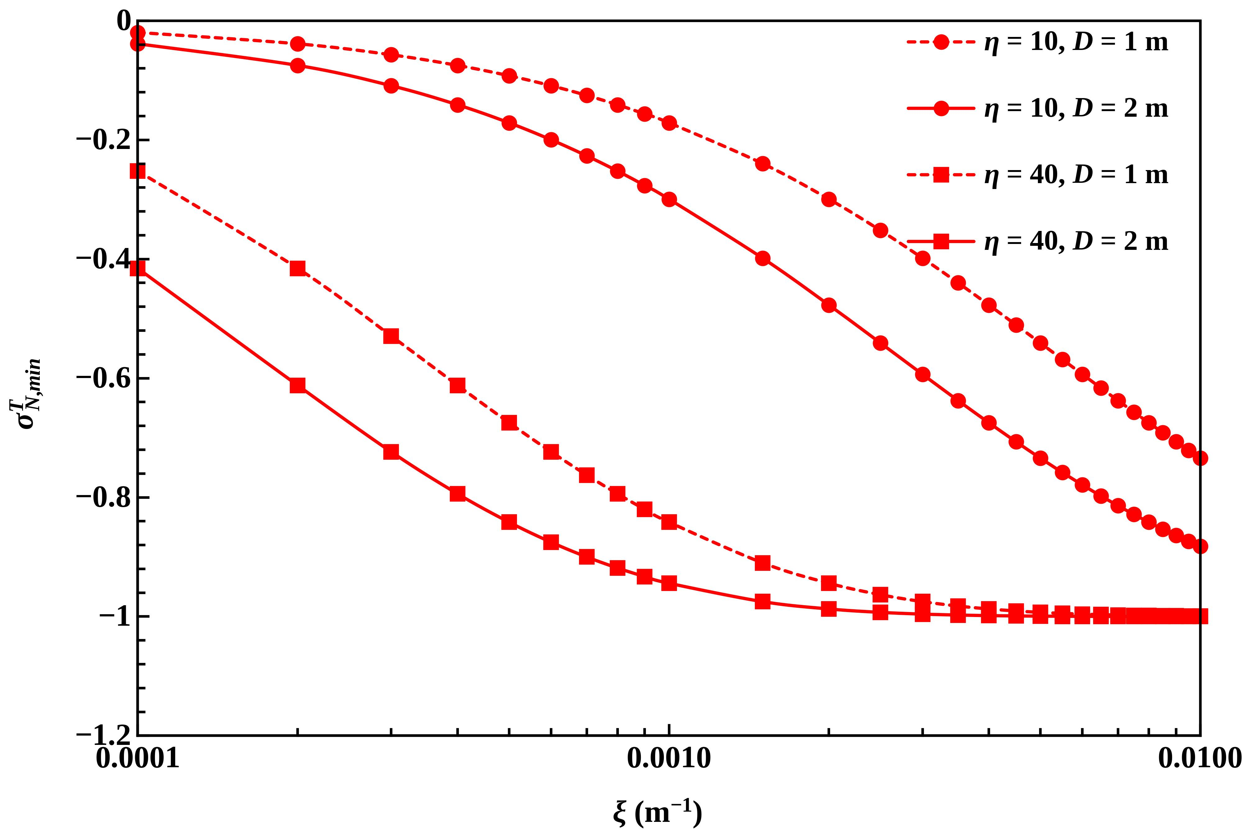
Figure 8 and Figure 9 show the maximum and minimum normalized thermal displacements and stresses, respectively. As expected, the displacement decreases with increasing , while stress increases with increasing . Moreover, the stress magnitude increases with increasing pile diameter and length-to-diameter ratio, while displacement decreases with increasing pile diameter and length-to-diameter ratio. Both null points, thermal and mechanical, are located in the pile tip in the case of an end-bearing pile.
Figure 1.
Dimensionless thermal and mechanical displacement vs. dimensionless depth for end-bearing piles.
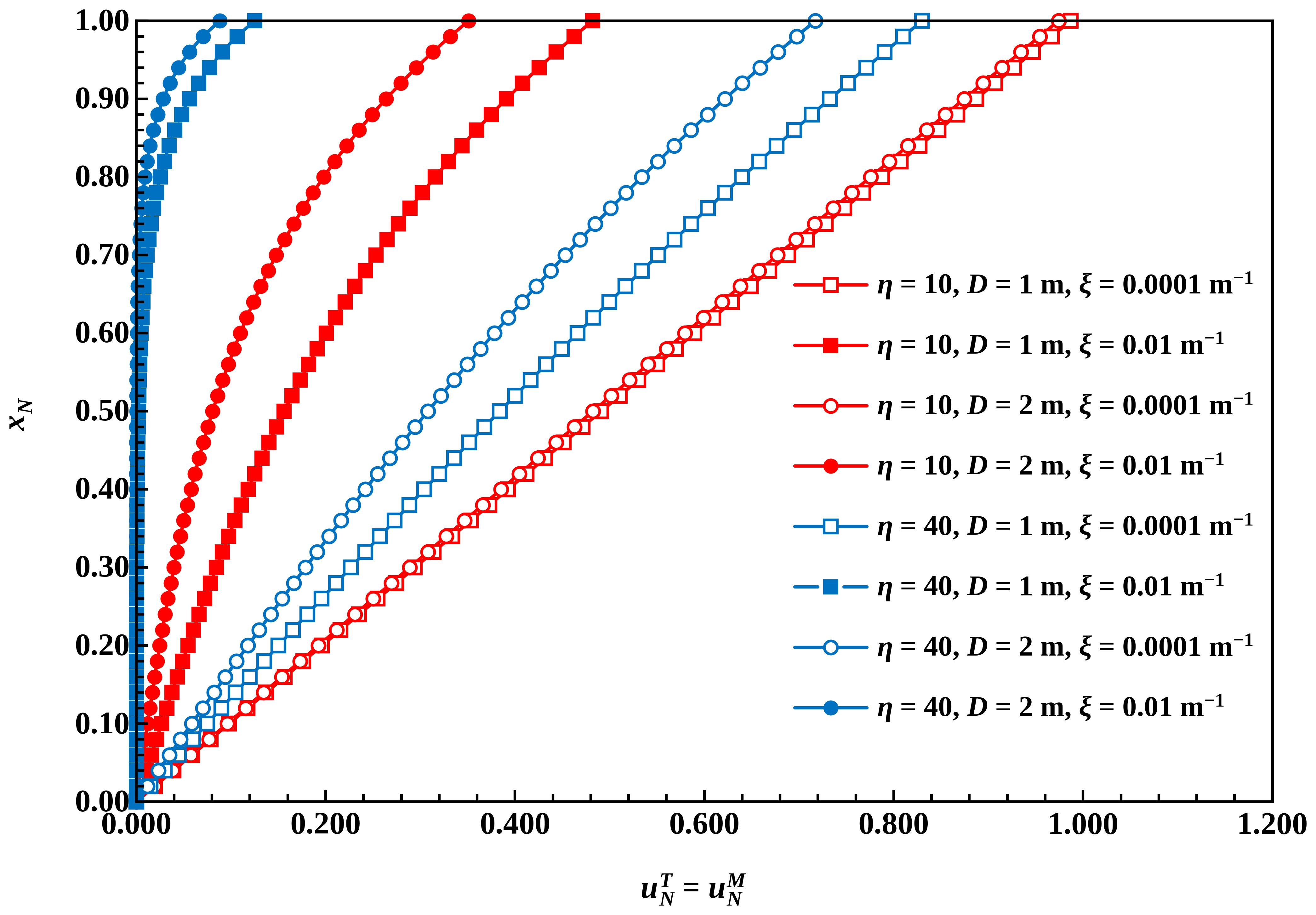
Figure 2.
Dimensionless thermal stress vs. dimensionless depth for end-bearing piles.
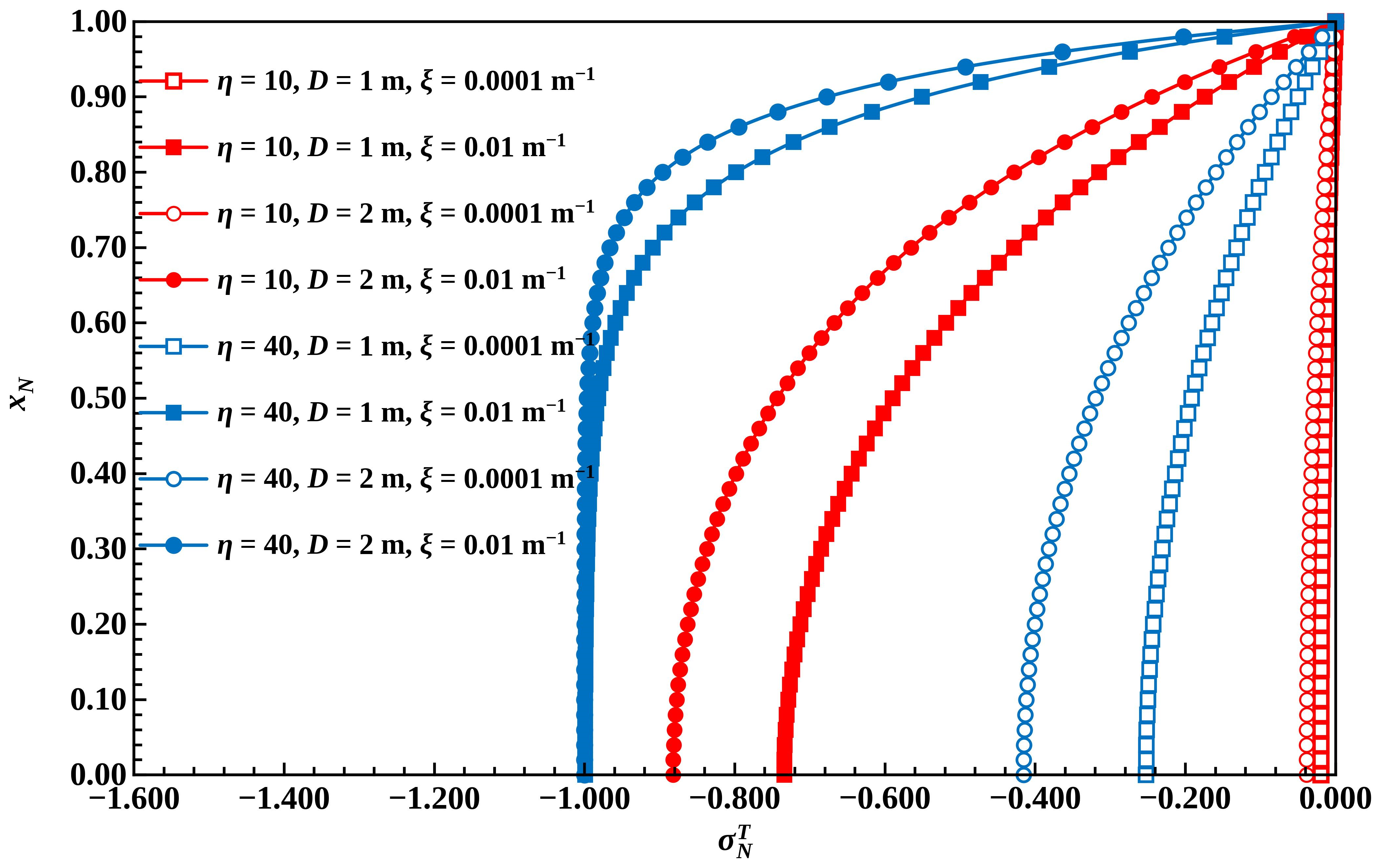
Figure 3.
Dimensionless mechanical stress vs. dimensionless depth for end-bearing piles.
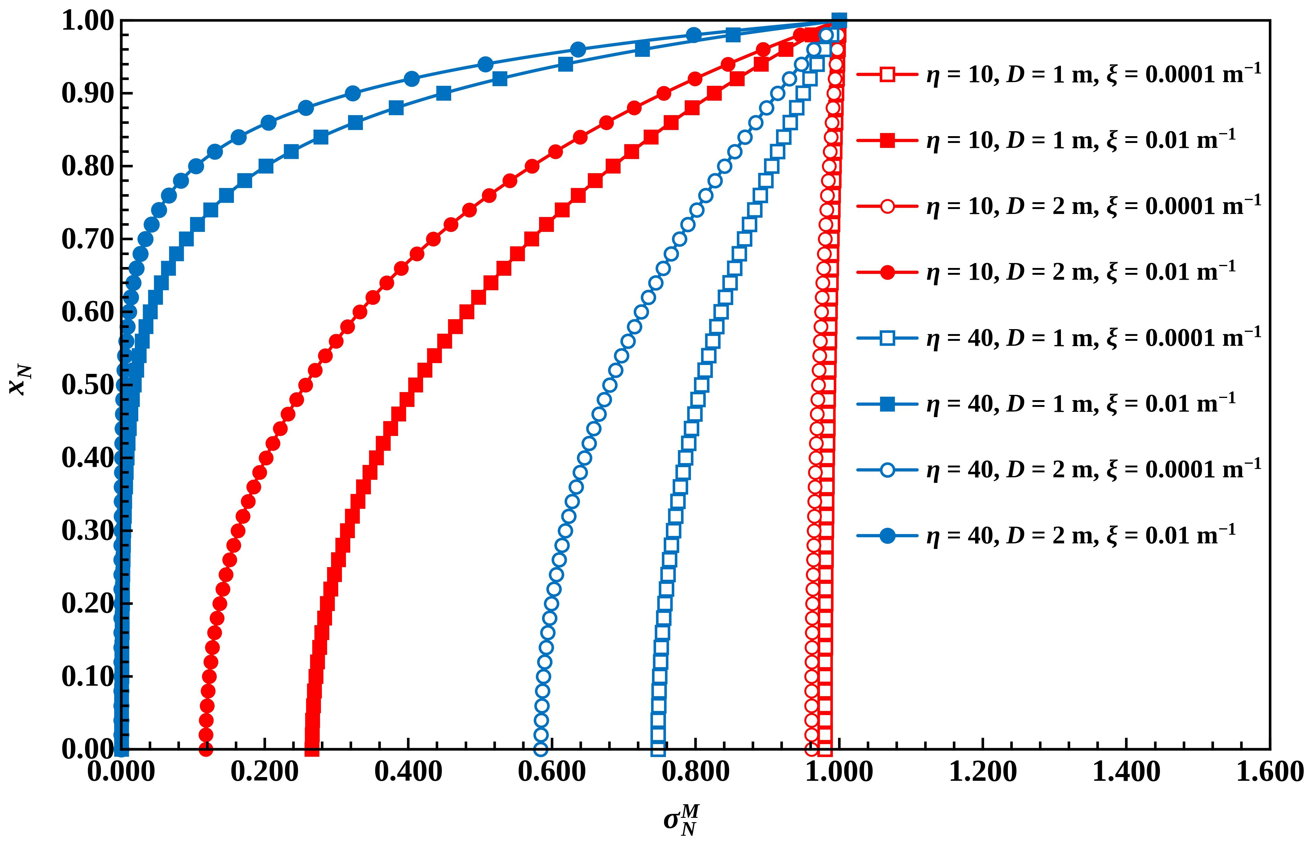
Figure 4.
Combined dimensionless displacement vs. dimensionless depth for end-bearing piles.
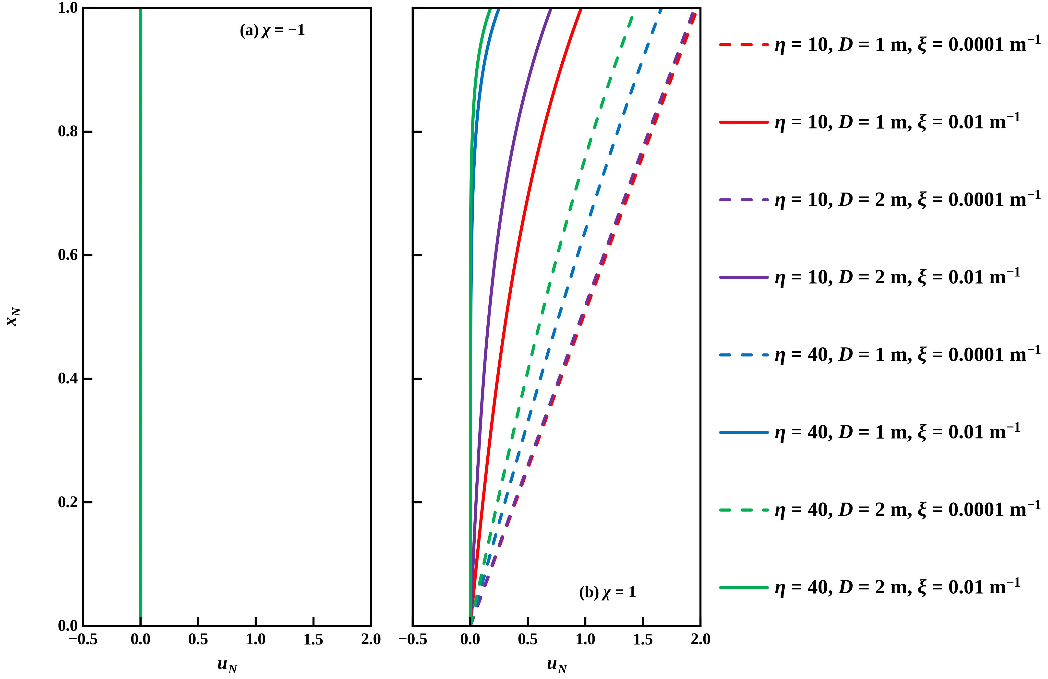
Figure 5.
Combined dimensionless stress vs. dimensionless depth for end-bearing piles.
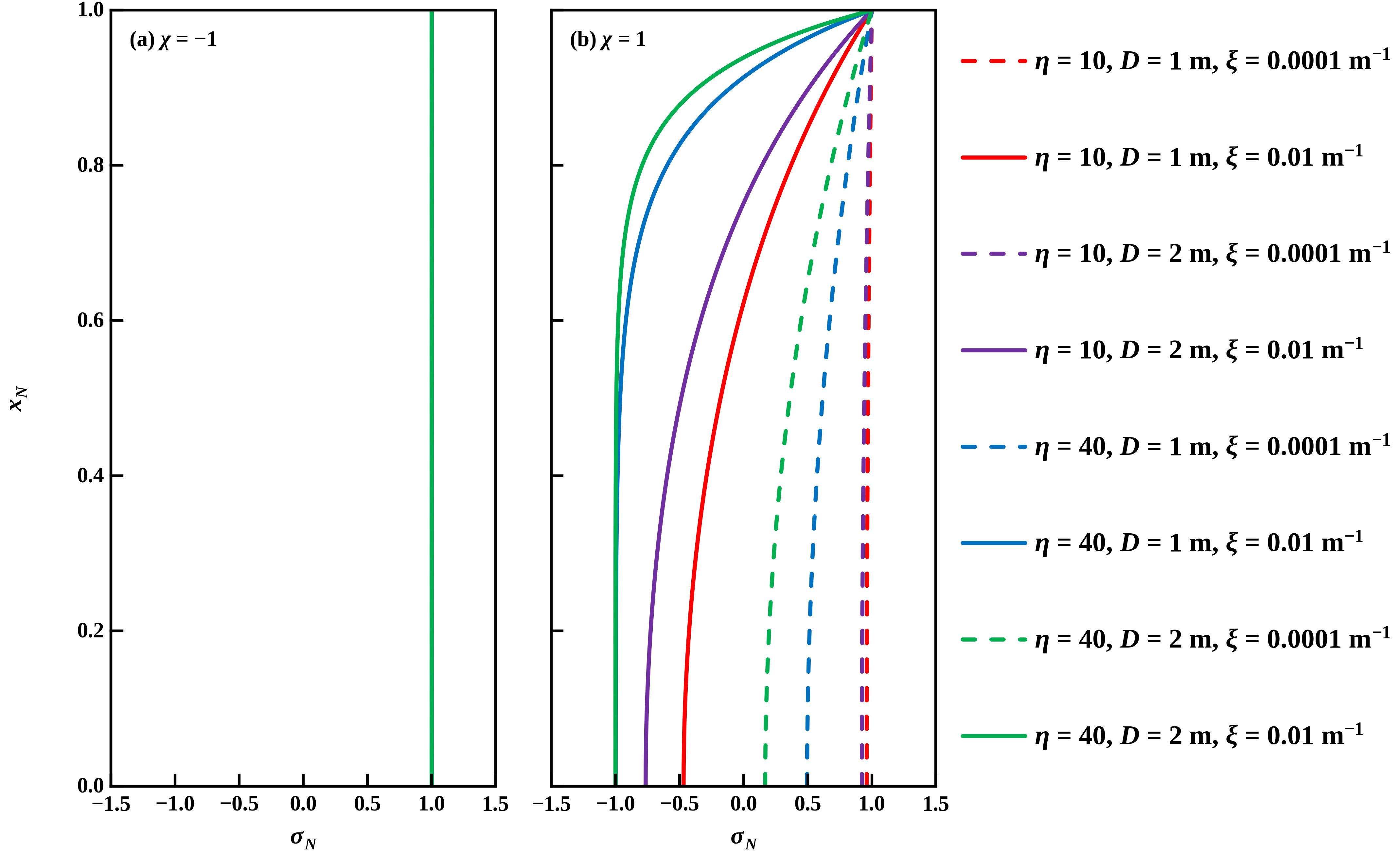
Figure 6.
Combined dimensionless displacement vs. dimensionless depth for selected values of χ, for end-bearing piles. Top row (heating), Bottom row (cooling).
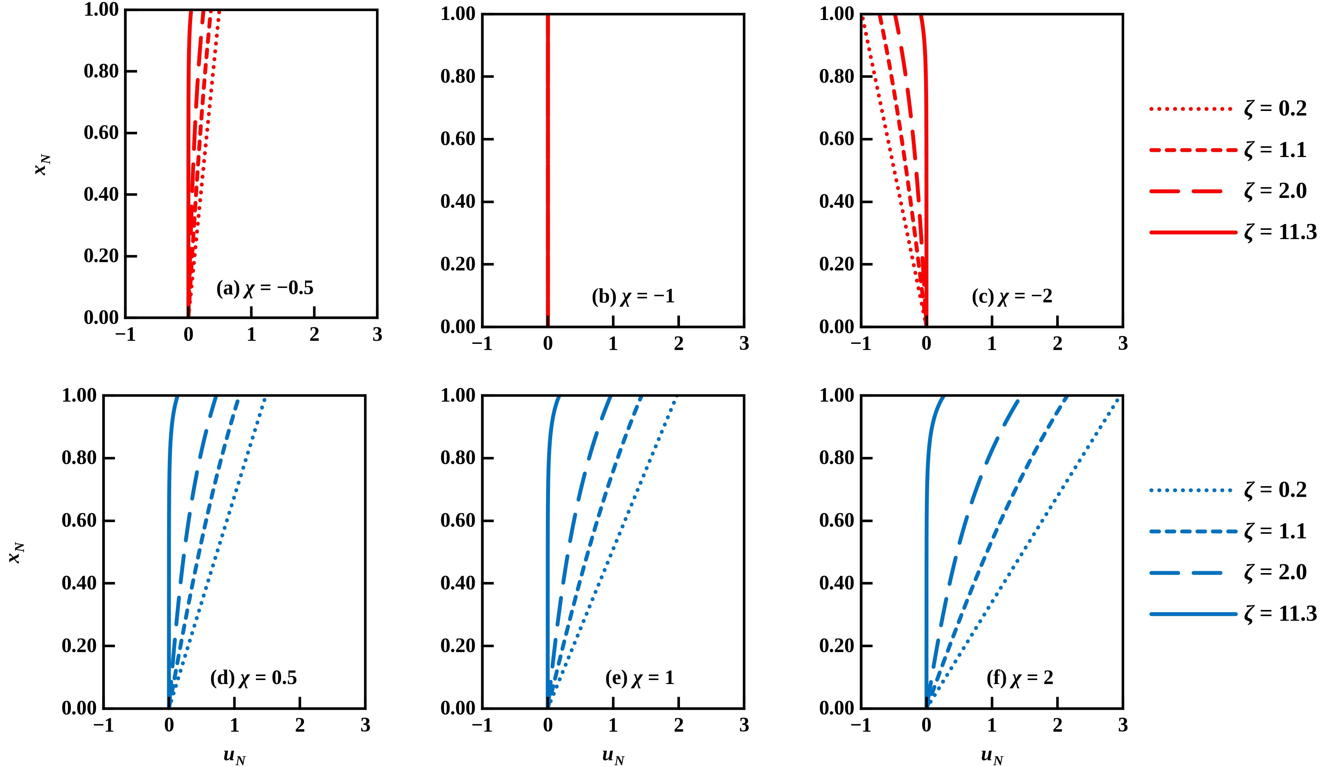
Figure 7.
Combined dimensionless stress vs. dimensionless depth for selected values of χ, for end-bearing piles. Top row (heating), Bottom row (cooling).
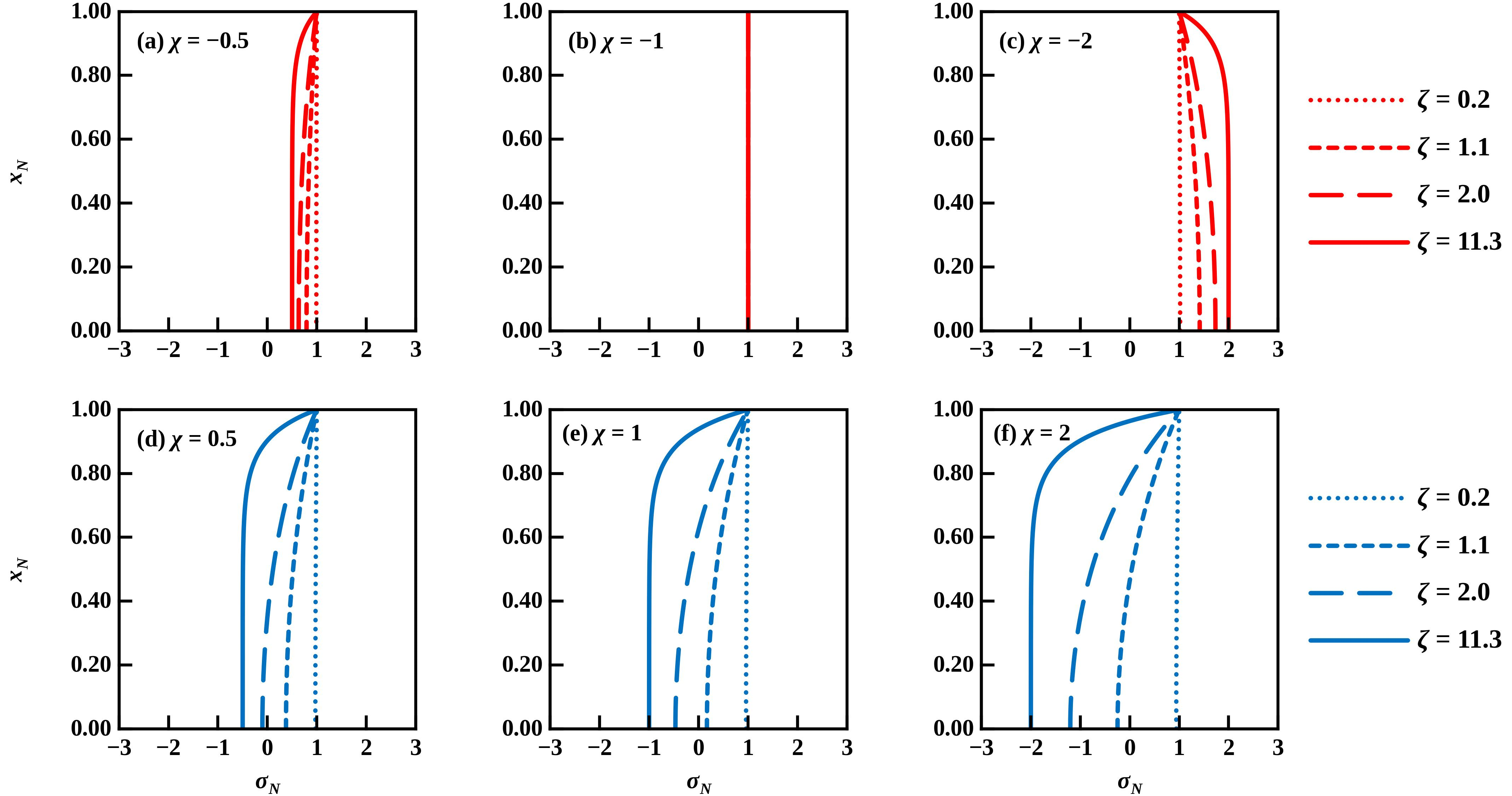
Figure 8.
Maximum dimensionless thermal and mechanical displacements vs. ξ (m−1) for end-bearing piles.
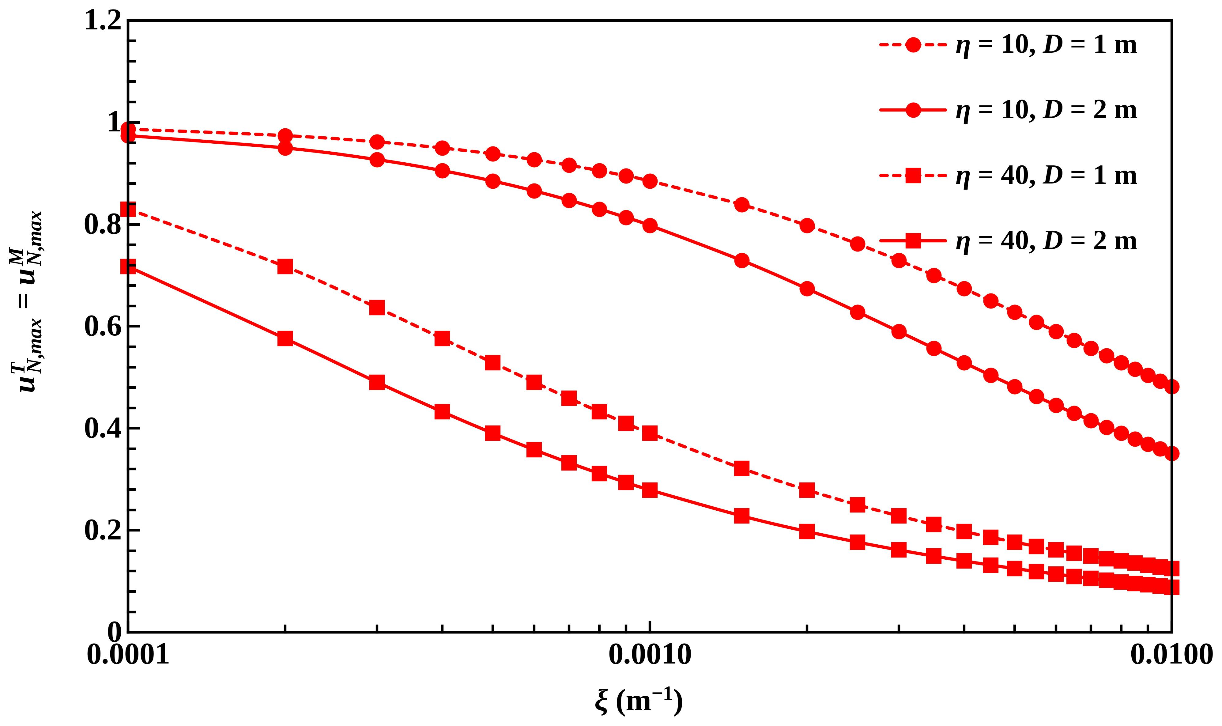
Figure 9.
Minimum dimensionless thermal stress vs. ξ (m−1) for end-bearing piles.
3.2. Fully Floating Pile
Figure 10 and Figure 11 depict the variations of dimensionless thermal and mechanical displacements vs. depth, respectively, while Figure 12 and Figure 13 show variations of normalized thermal and mechanical stresses. The thermal stress in the bottom part of the pile is a mirror image of the stress in the top half. Due to the bottom and top boundary conditions requiring zero thermal stress, the maximum magnitude of thermal stress develops at the mid-length (Figure 12), and the largest magnitude of this stress corresponds to the largest value as discussed previously. Equation (36) indicates that the thermal null point is at the mid-length, resulting in zero thermal displacement at this location. This results in positive normalized displacement above the null point and negative normalized displacement below it. Otherwise, the effect of value on the magnitude of thermal stress and displacement is the same as in the case of the end-bearing pile. It is also noted that the maximum thermal displacement in this case is half of the corresponding maximum thermal displacement observed in the end-bearing pile. Normalized mechanical displacement is extremely large for the smallest value of (=0.2) because this is a fully floating pile. However, the displacement decreases first gradually with increasing , and subsequently quickly converges to significantly smaller values. Trends observed in the normalized mechanical stress (Figure 13) are similar to those exhibited by the end-bearing pile (Figure 3), except in this case, the tip stress is zero.
Figure 14 and Figure 15 show the normalized combined displacement and stress for , with heating (χ = −1) in panel (a) and cooling (χ = 1) in panel (b). Extremely large magnitudes of displacements are observed for the lowest values in case of heating and cooling. In the case of heating for , as expected, the combined displacement at the pile head is zero, but it is very large at the pile tip due to the shape of the normalized thermal displacement curve discussed above (Figure 11). In the case of cooling for , the extremely large displacement occurs at the pile head with corresponding displacement of zero at the pile tip (Figure 14b). Combined normalized stress has the same features as in the case of an end-bearing pile, except that it is zero at the pile tip due to the boundary condition of the fully floating pile (Figure 15). Specifically, the magnitudes of maximum combined stresses for heating and cooling are equal to one (Figure 15a,b).
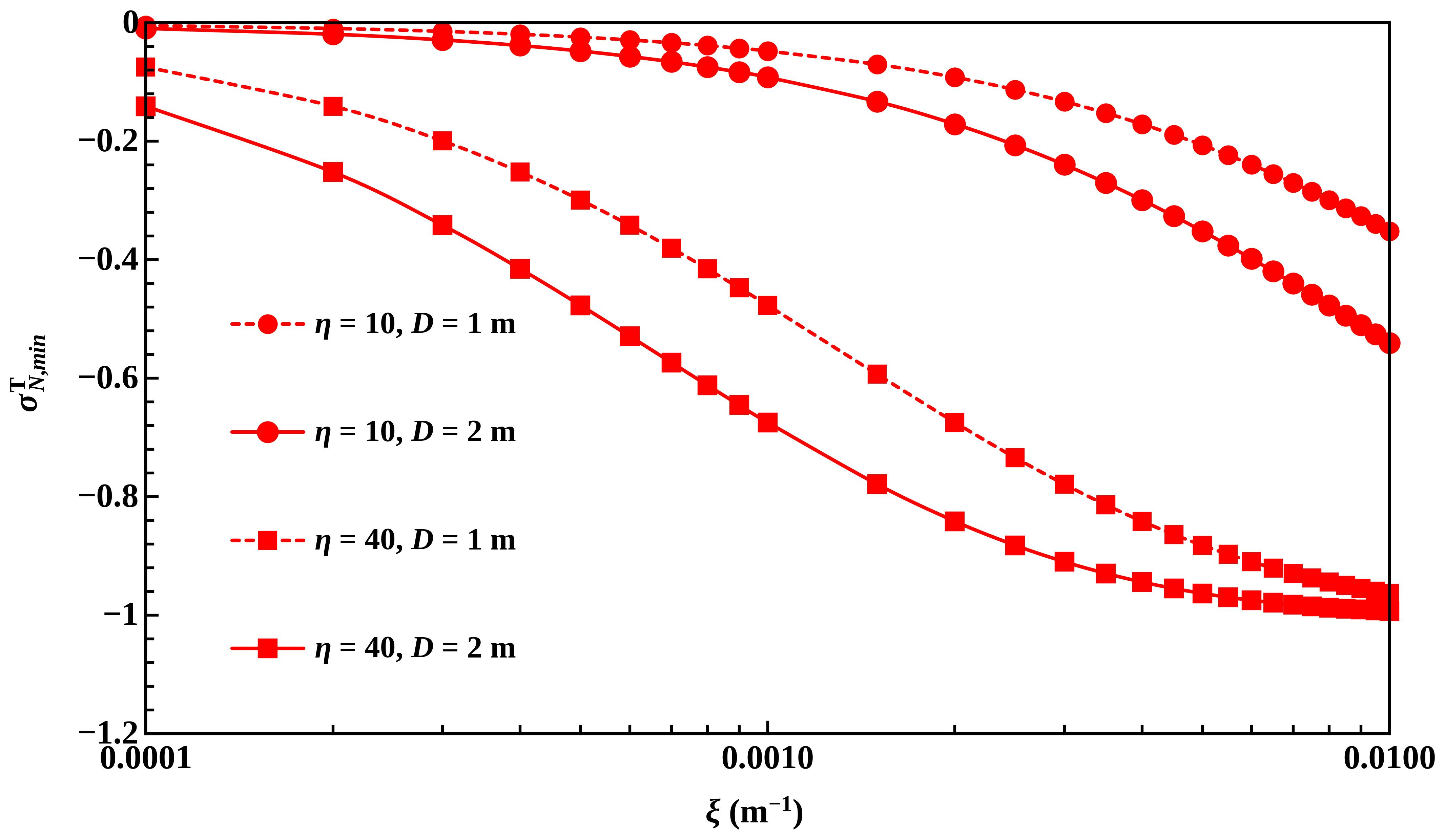
Figure 16 and Figure 17 depict normalized combined displacements and stress for additional values of and . Significantly large displacement magnitudes are observed for the lowest value. For the smallest amount of heating the magnitude of normalized displacement is smaller at the pile head than at the pile tip, because the magnitudes of mechanical and thermal displacements add at the pile tip and subtract at the pile head. With the further increase in the amount of heating, the combined thermal point emerges at the pile head for and moves downward for . In the case of cooling magnitudes of thermal and mechanical displacements, add in the top half of the pile and subtract in the bottom part, thus resulting in the emergence of a combined null point at the pile tip for and its subsequent movement upwards for In the case of a fully floating pile, the stress magnitude at the tip is always equal to zero, resulting in a different response from the end-bearing pile. However, the combined normalized stress response becomes dominated by the thermal response at , thus resulting in the maximum magnitude of combined stress being achieved for the largest value of (=11.3) and the magnitude of the combined stress increases even further for . The maximum predicted normalized tensile stress magnitude is 2, for , indicating that proper steel reinforcement is required. Finally, Figure 18 and Figure 19 depict the maximum normalized thermal and mechanical displacements and the maximum magnitude of normalized thermal stress. A similar pattern to the end-bearing pile is observed, i.e., both displacements decrease with increasing and values, while the maximum magnitude of stress increases with increasing and values.
Figure 10.
Dimensionless thermal displacement vs. dimensionless depth for fully floating piles.
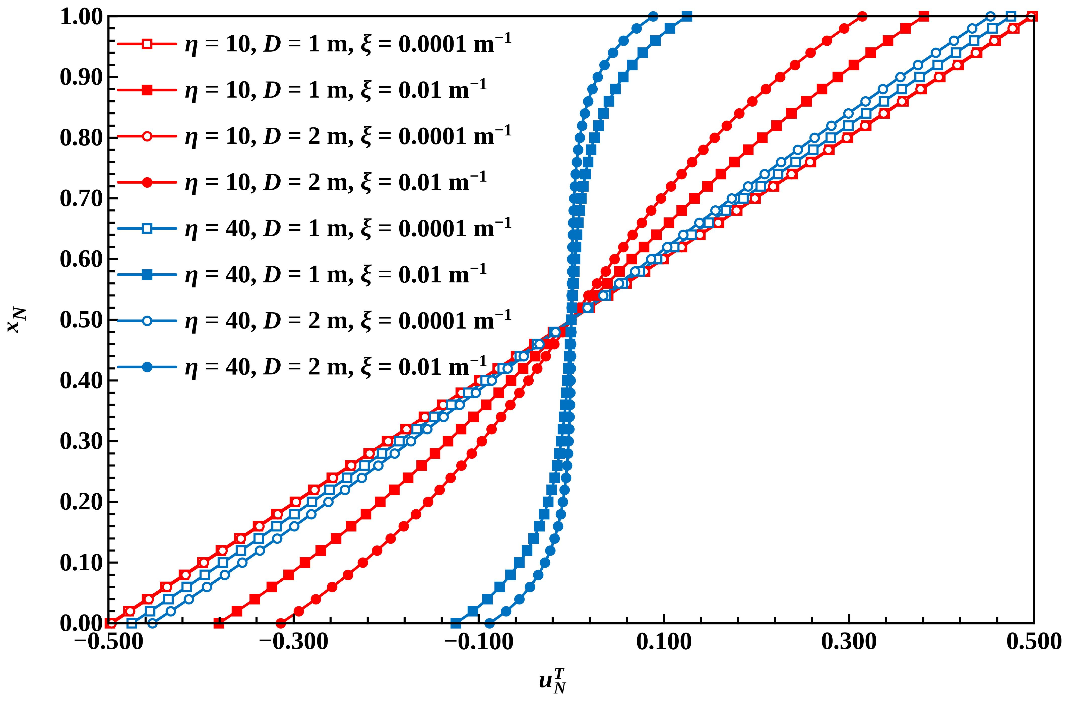
Figure 11.
Dimensionless mechanical displacement vs. dimensionless depth for fully floating piles.
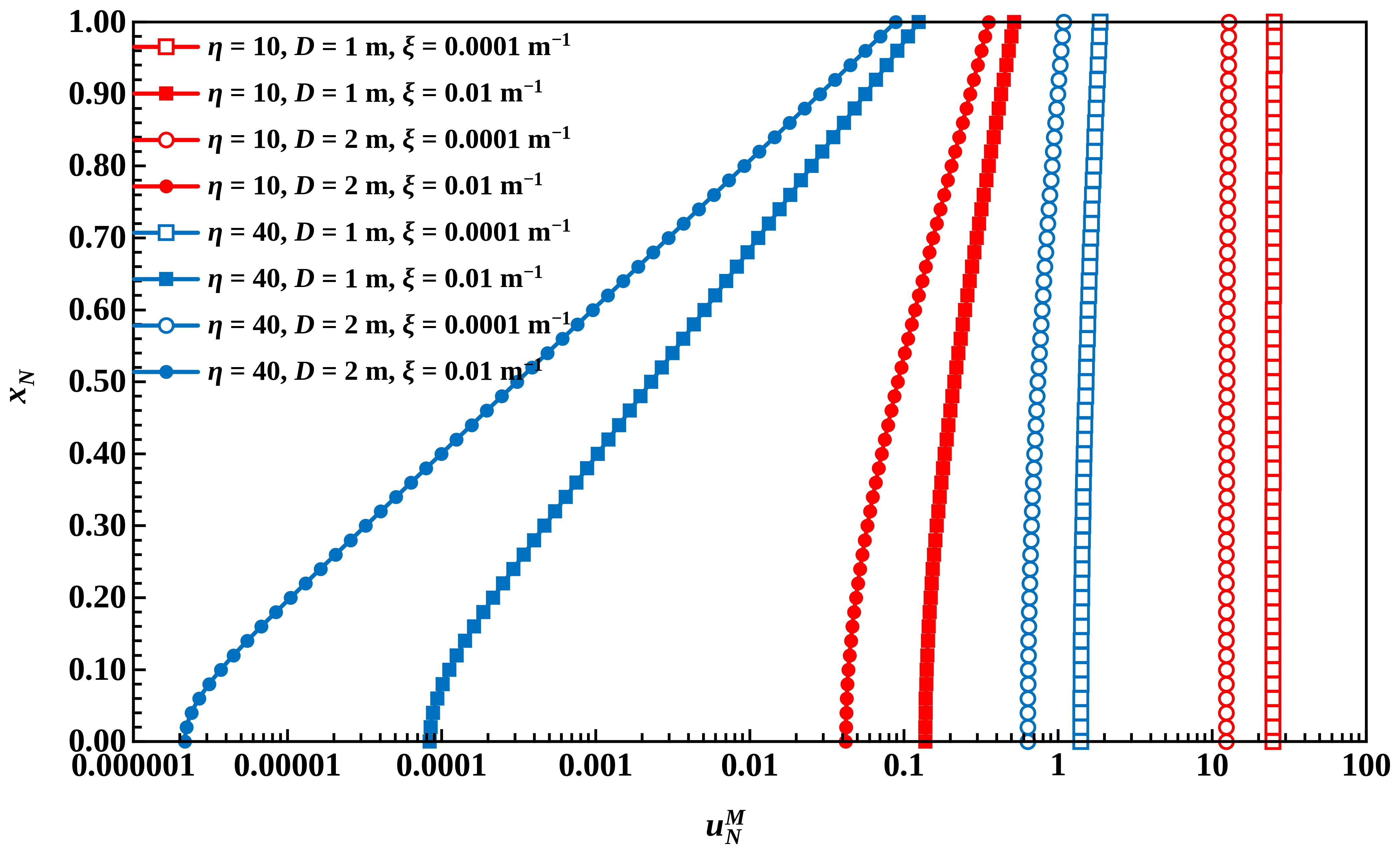
Figure 12.
Dimensionless thermal stress vs. dimensionless depth for fully floating piles.
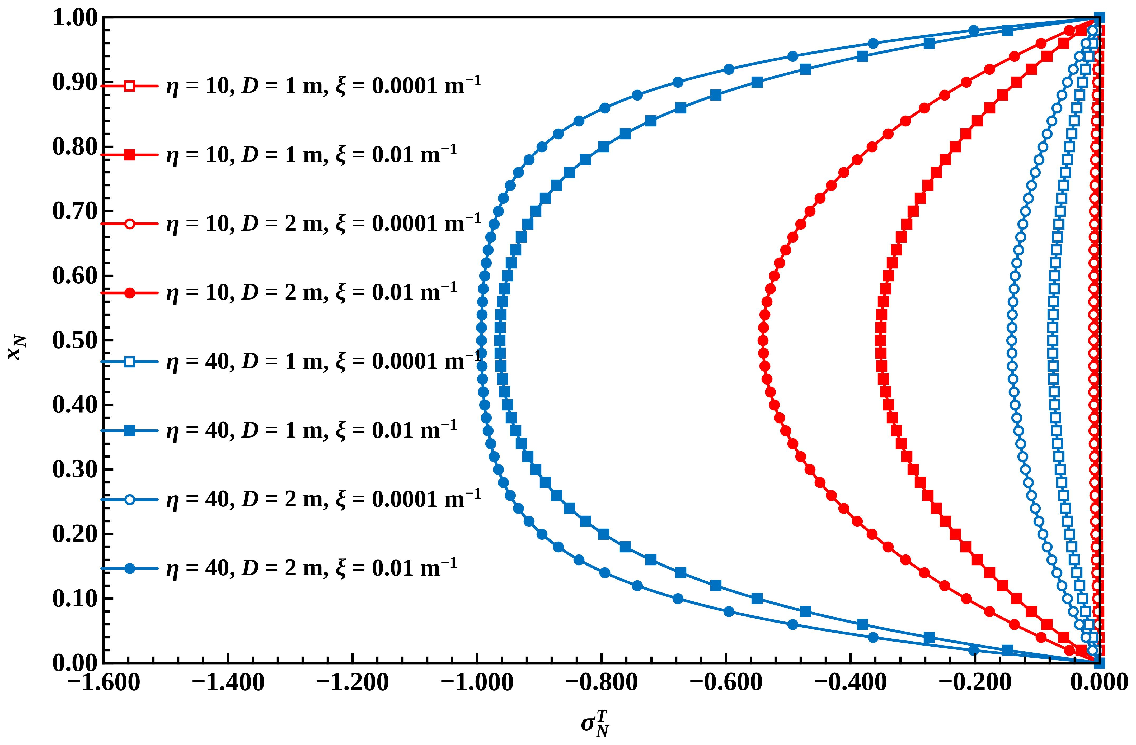
Figure 13.
Dimensionless mechanical stress vs. dimensionless depth for fully floating piles.
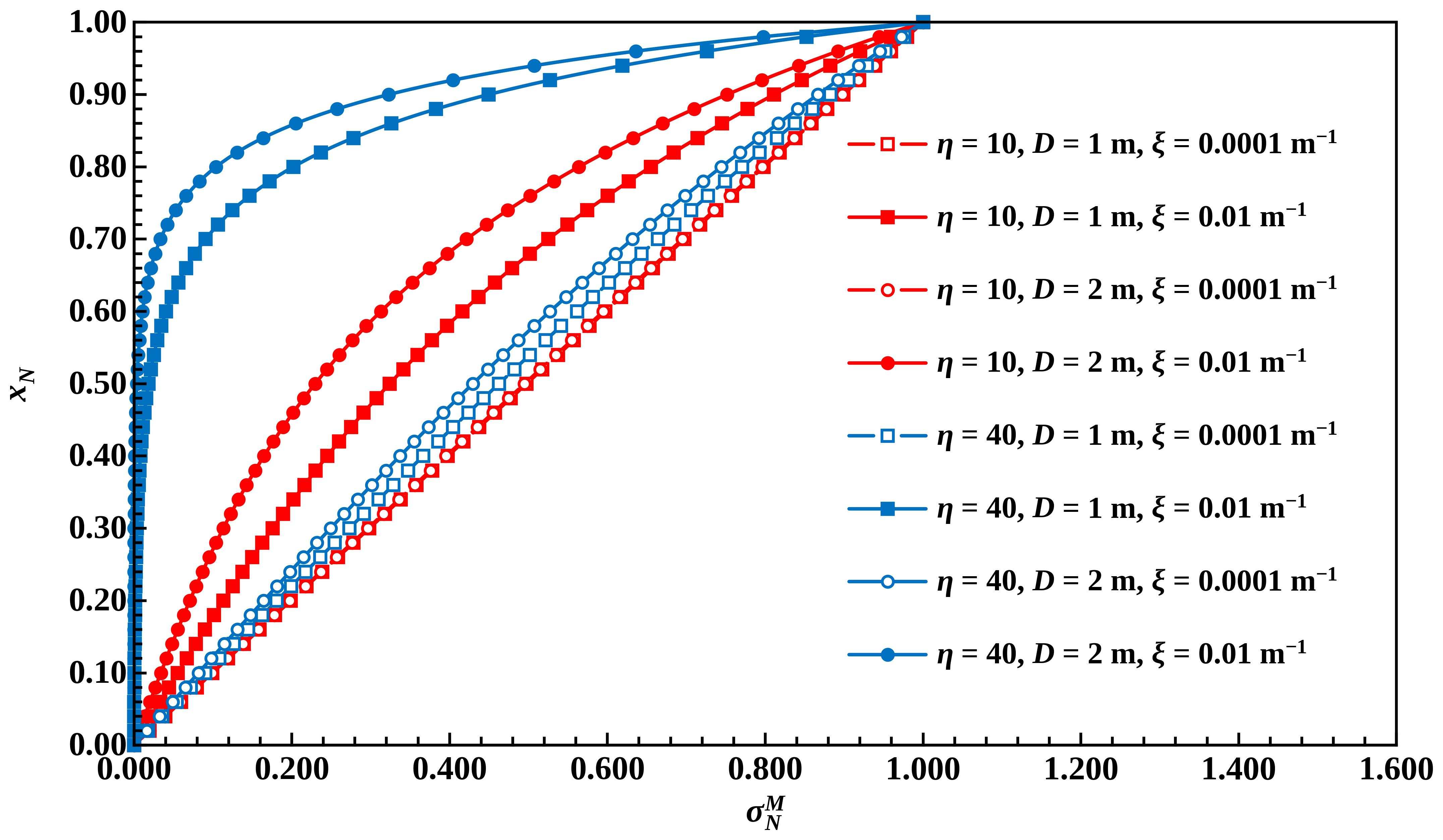
Figure 14.
Combined dimensionless displacement vs. dimensionless depth for fully floating piles.
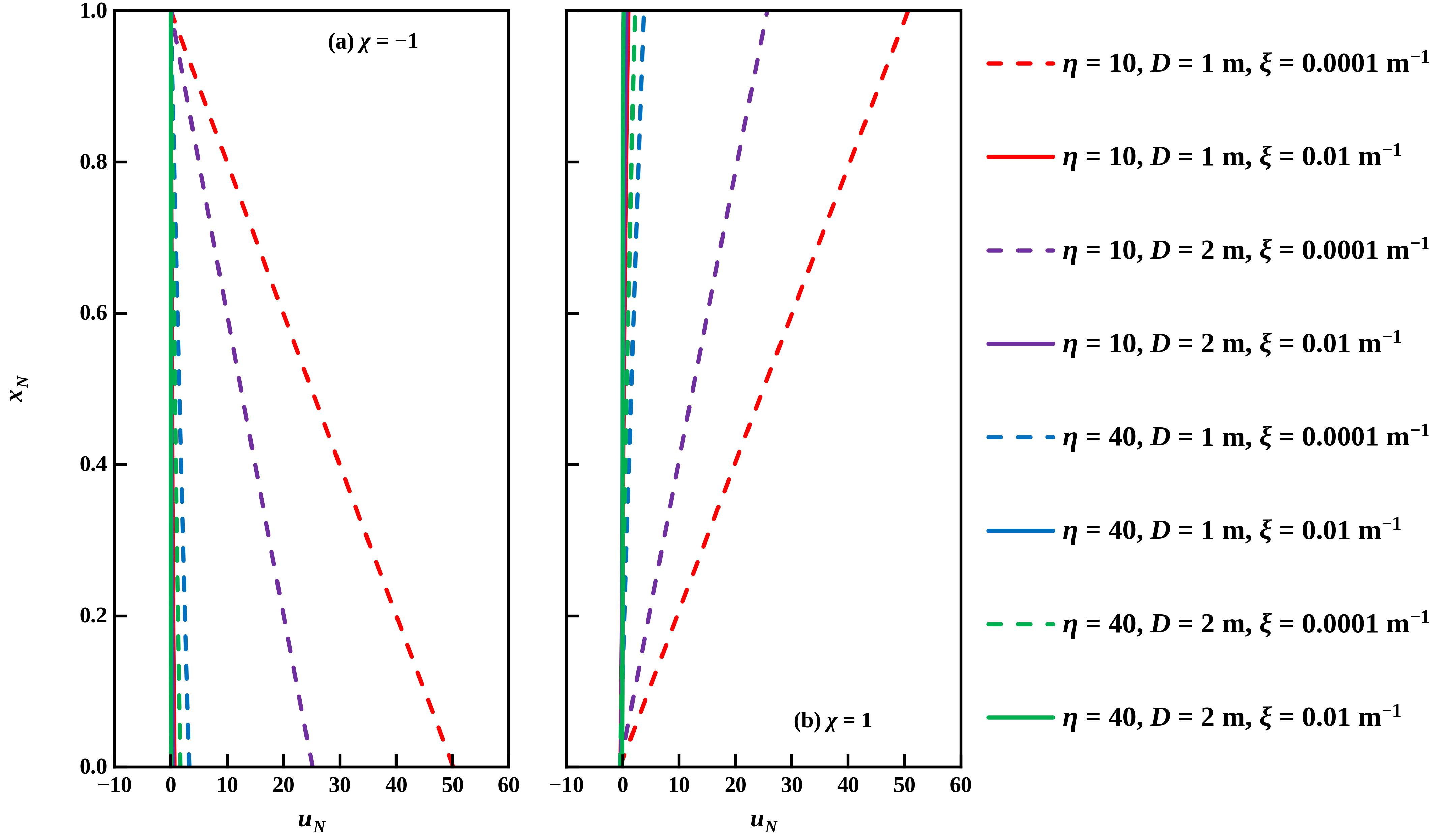
Figure 15.
Combined dimensionless stress vs. dimensionless depth for fully floating piles.
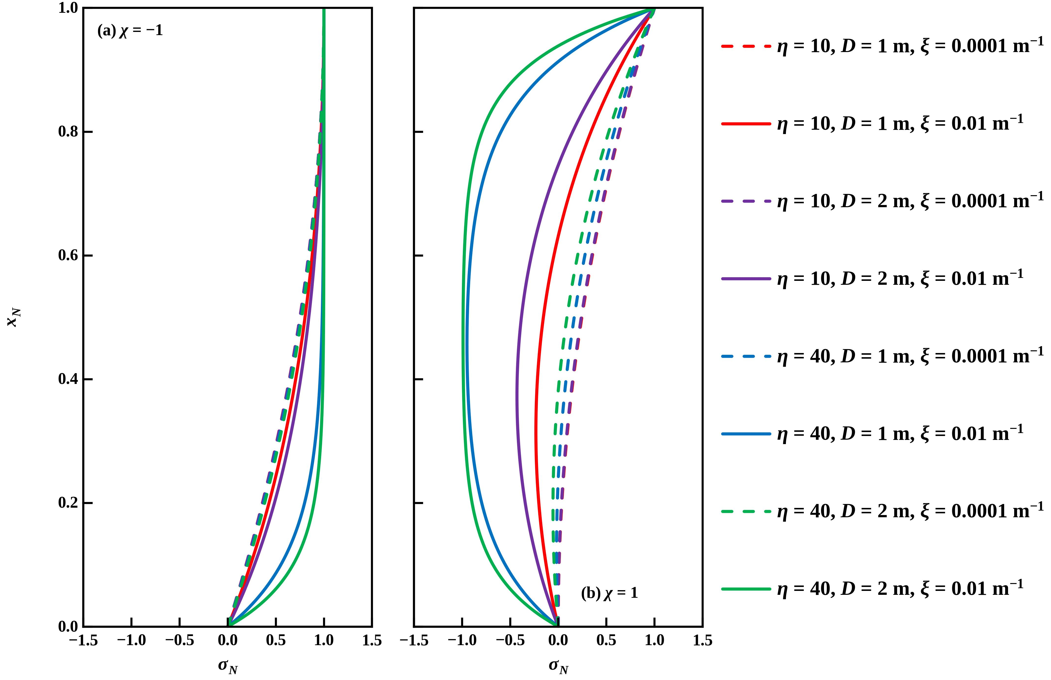
Figure 16.
Combined dimensionless displacement vs. dimensionless depth for selected values of χ, for fully floating piles. Top row (heating), Bottom row (cooling).
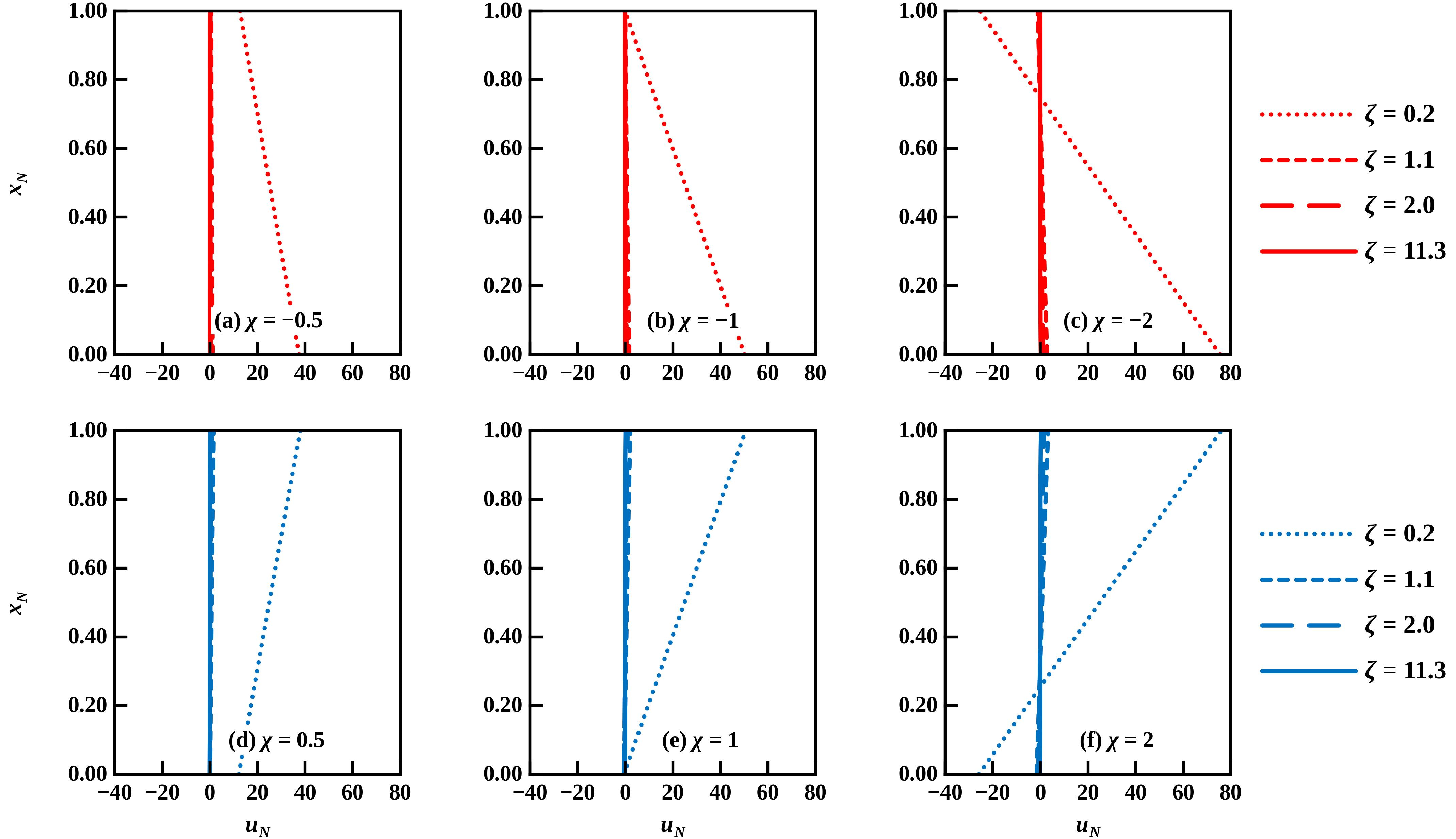
Figure 17.
Combined dimensionless stress vs. dimensionless depth for all selected values of χ, for fully floating piles. Top row (heating), Bottom row (cooling).
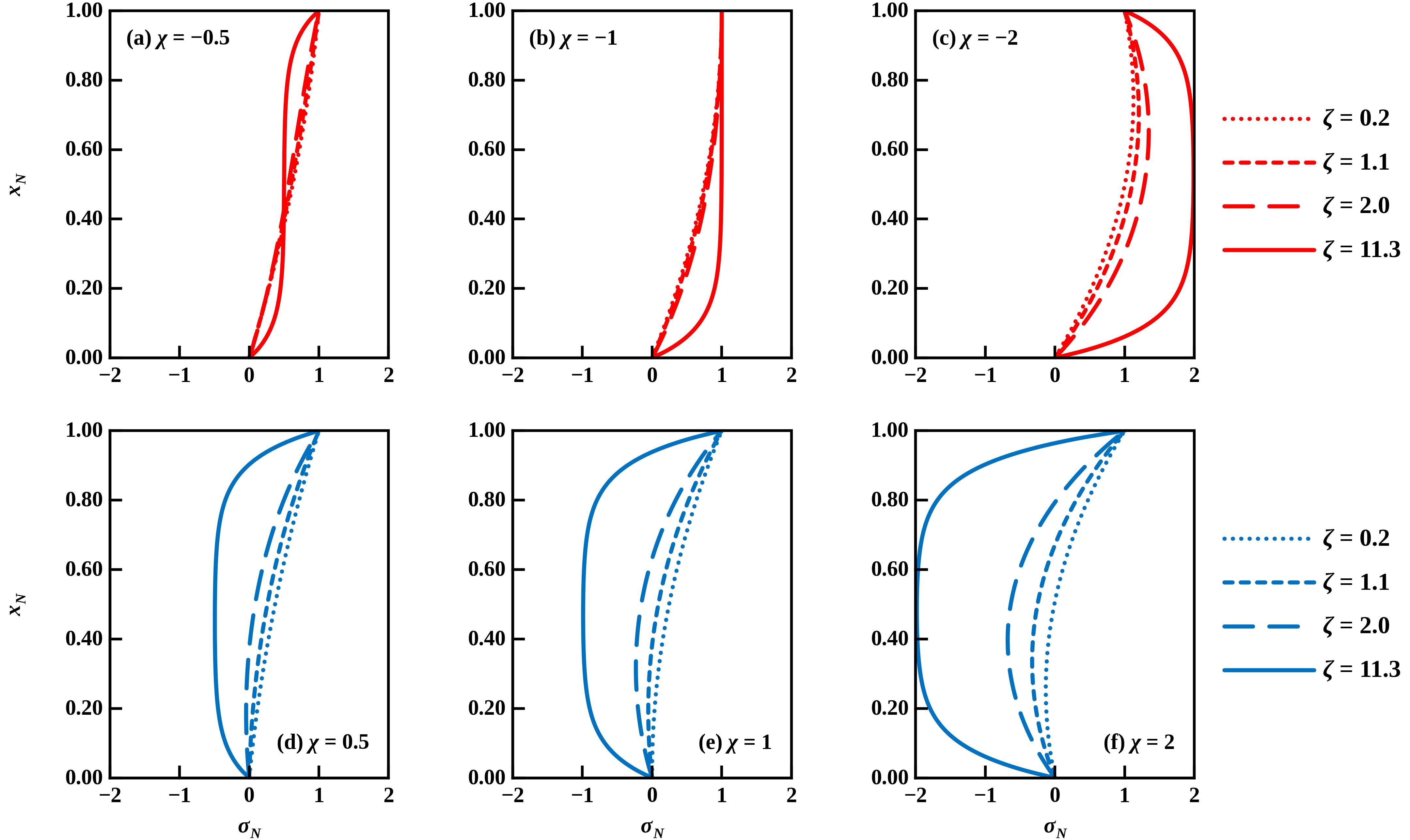
Figure 18.
Maximum dimensionless thermal and mechanical displacements vs. ξ (m−1) for fully floating piles.
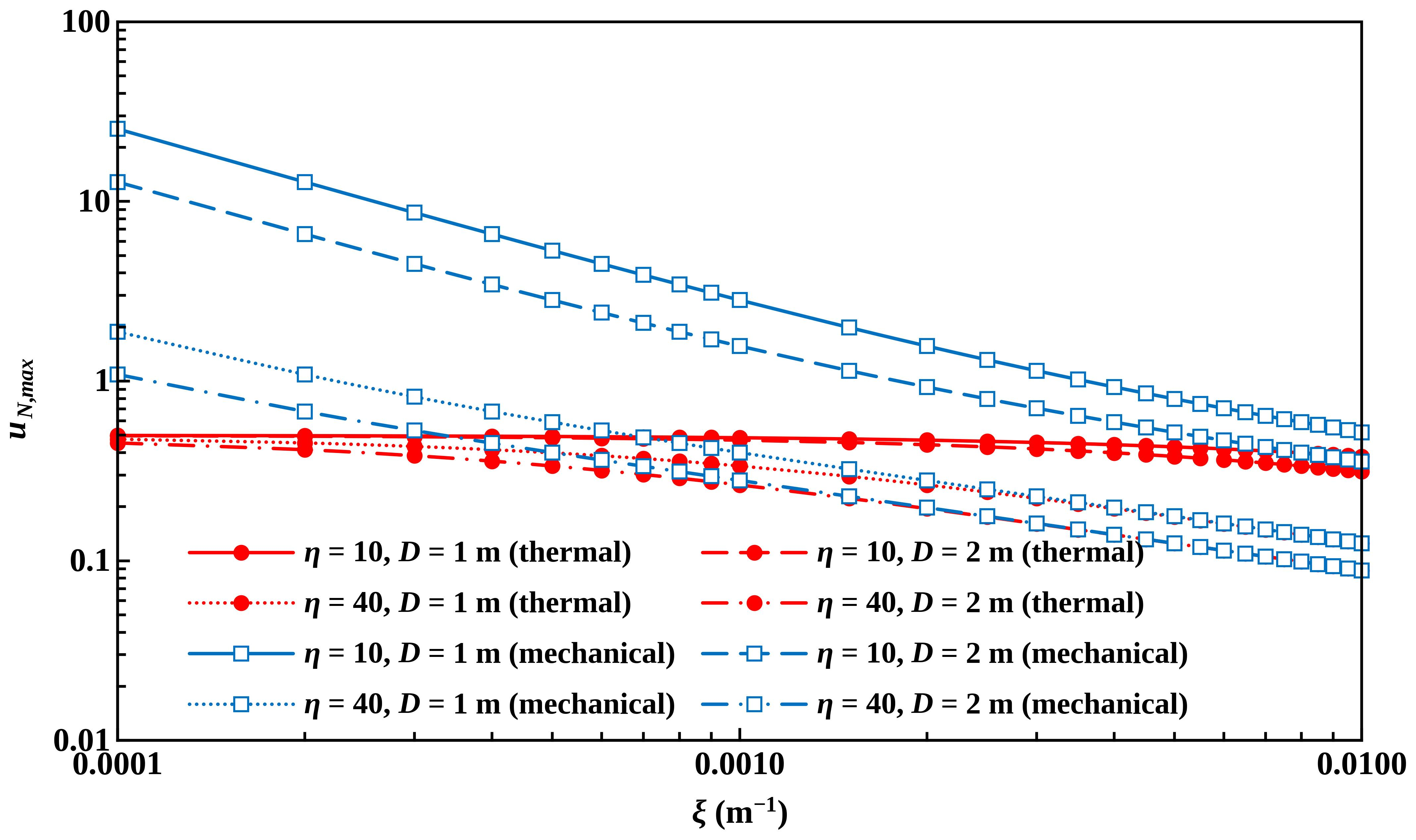
Figure 19.
Minimum dimensionless thermal stress vs. ξ (m−1) for fully floating piles.
3.3. Semi-Floating Pile
Figure 20, Figure 21, Figure 22, Figure 23, Figure 24, Figure 25, Figure 26, Figure 27, Figure 28, Figure 29, Figure 30, Figure 31 and Figure 32 show the response of a semi-floating pile, including two different values of corresponding to 0.1 m−1 and 1 m−1. Normalized thermal displacement (Figure 20) indicates that the lower the value of the more the pile resembles a fully floating pile in the case of larger values, thus having a thermal null point located near the mid-length. With increasing the thermal null point moves closer to the tip, and the pile more closely resembles a semi-floating pile. However, for small values regardless of the value, the semi-floating pile starts to resemble the end-bearing pile. The normalized mechanical displacement shown in Figure 21 reflects the thermal behavior, as it behaves more like a fully floating pile for the same values of controlling parameters as under thermal loading. Finally, the smallest value results in the largest normalized displacement for both thermal and mechanical responses.
The normalized stress response is shown in Figure 22 and Figure 23 for thermal and mechanical loading, respectively. Specifically, the maximum magnitude of normalized thermal stress occurs near the mid-length for larger values and 0.1 m−1, while the largest magnitude of thermal stress occurs closer to the tip for 1 m−1. This behavioral pattern is also reflected in Figure 23b, which depicts the normalized mechanical stress, which is closer for the fully floating pattern.
Figure 24 and Figure 25 show combined normalized displacements and stresses for , for ξb = 0.1 m−1 (panels (a) and (c)) and ξb = 1 m−1 (panels (b) and (d)), with heating (χ = −1) in the top row and cooling (χ = 1) in the bottom row. As expected, displacements are larger in the case of cooling, especially for low values (Figure 24c,d). Furthermore, for the end-bearing pattern, i.e., lower values the combined stress in heating is nearly constant with depth and equal to 1 (Figure 25a,b), as in the case of end-bearing piles (Figure 5a). Otherwise, for larger values the fully floating and semi-floating patterns are reproduced, thus resulting in the maximum normalized magnitude of combined stress in cooling equal to one (Figure 25c,d).
Figure 26 shows the normalized combined displacements for χ values of −2, −1, −0.5, 0.5, 1, and 2, and 0.1 m−1 The smallest magnitude of heating ( = −0.5) decreases mechanical head displacement by the same amount by which it increases tip displacement, thus resulting in the constant displacement vs. depth for the smallest . As the amount of heating is increased, the displacement at the head is further decreased, resulting in the emergence of a combined null point at the pile head for = −1, and movement of the null point further down for = −2. However, during cooling, the magnitude of normalized displacement at the pile head increases, while that at the pile tip decreases. Figure 28 shows similar patterns of displacement as observed in Figure 26, but they are now smaller due to the higher value, which is 1 m−1.
Figure 27 depict normalized combined stress for χ values including −2, −1, −0.5, 0.5, 1, and 2, for 0.1 m−1 and 1 m−1. It is similar to Figure 29, which depicts normalized stresses for the same selection of χ values but with 1 m−1. Stress patterns are similar, but the stress response for a higher value of is more similar to that of an end-bearing pile; for example, in Figure 29b, normalized stress is nearly constant with depth and equal to 1, while the corresponding stress in Figure 27b differs more from 1 near the pile tip. Figure 30 and Figure 31 show the maximum normalized thermal and mechanical displacements, respectively. As expected, all normalized displacements decrease as ζ increases. However, for 0.01 m−1, maximum mechanical displacements are slightly smaller for 1 m−1 than for 0.1 m−1 because the former pile response resembles the end-bearing pile. In both cases, the maximum magnitude of normalized displacement occurs at the pile head. Finally, Figure 32 depicts the maximum magnitude of normalized thermal stress, which, as expected, increases with increasing value.
Figure 20.
Dimensionless thermal displacement vs. dimensionless depth for semi-floating piles.
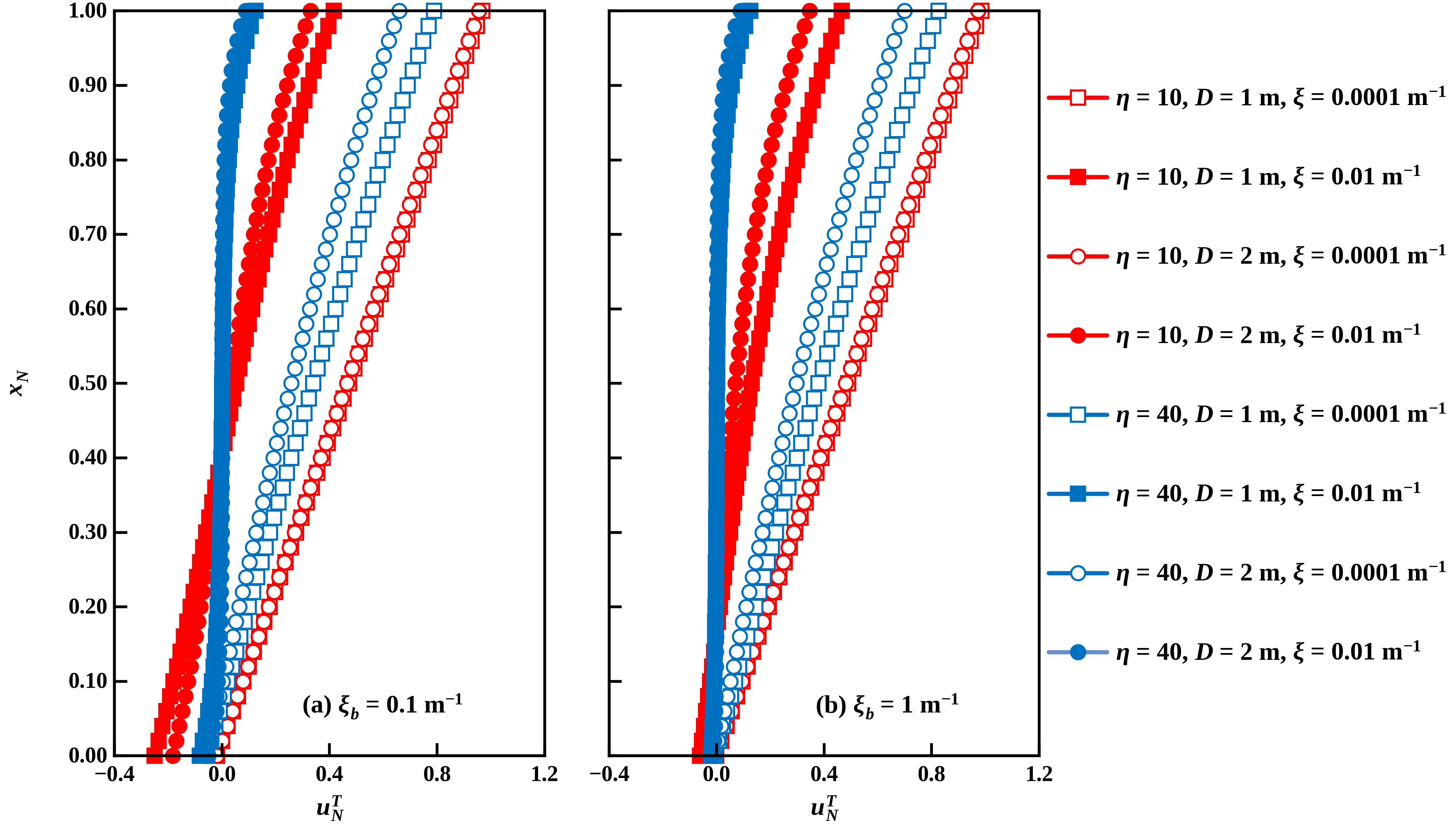
Figure 21.
Dimensionless mechanical displacement vs. dimensionless depth for semi-floating piles.
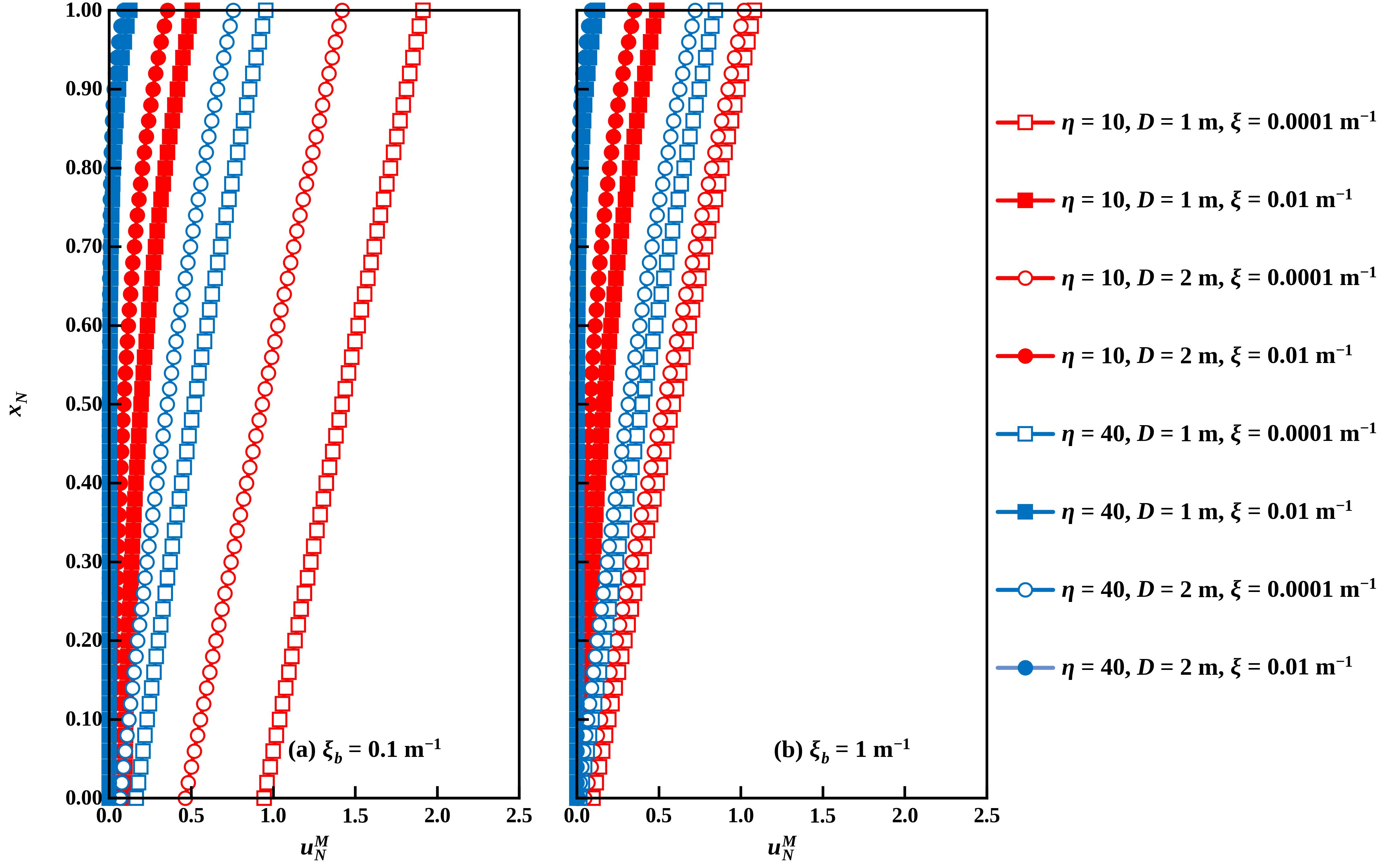
Figure 22.
Dimensionless thermal stress vs. dimensionless depth for semi-floating piles.
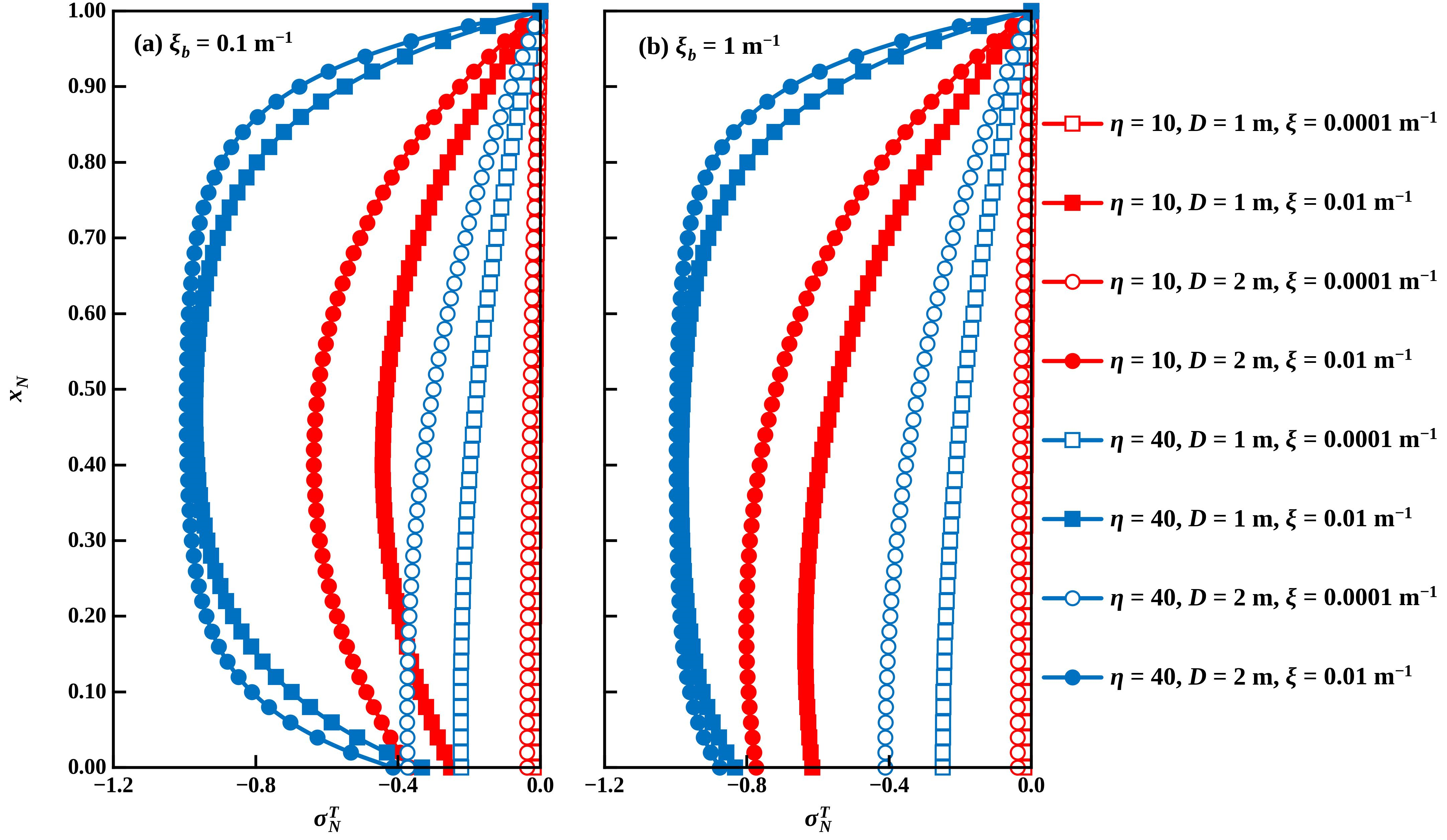
Figure 23.
Dimensionless mechanical stress vs. dimensionless depth for semi-floating piles.
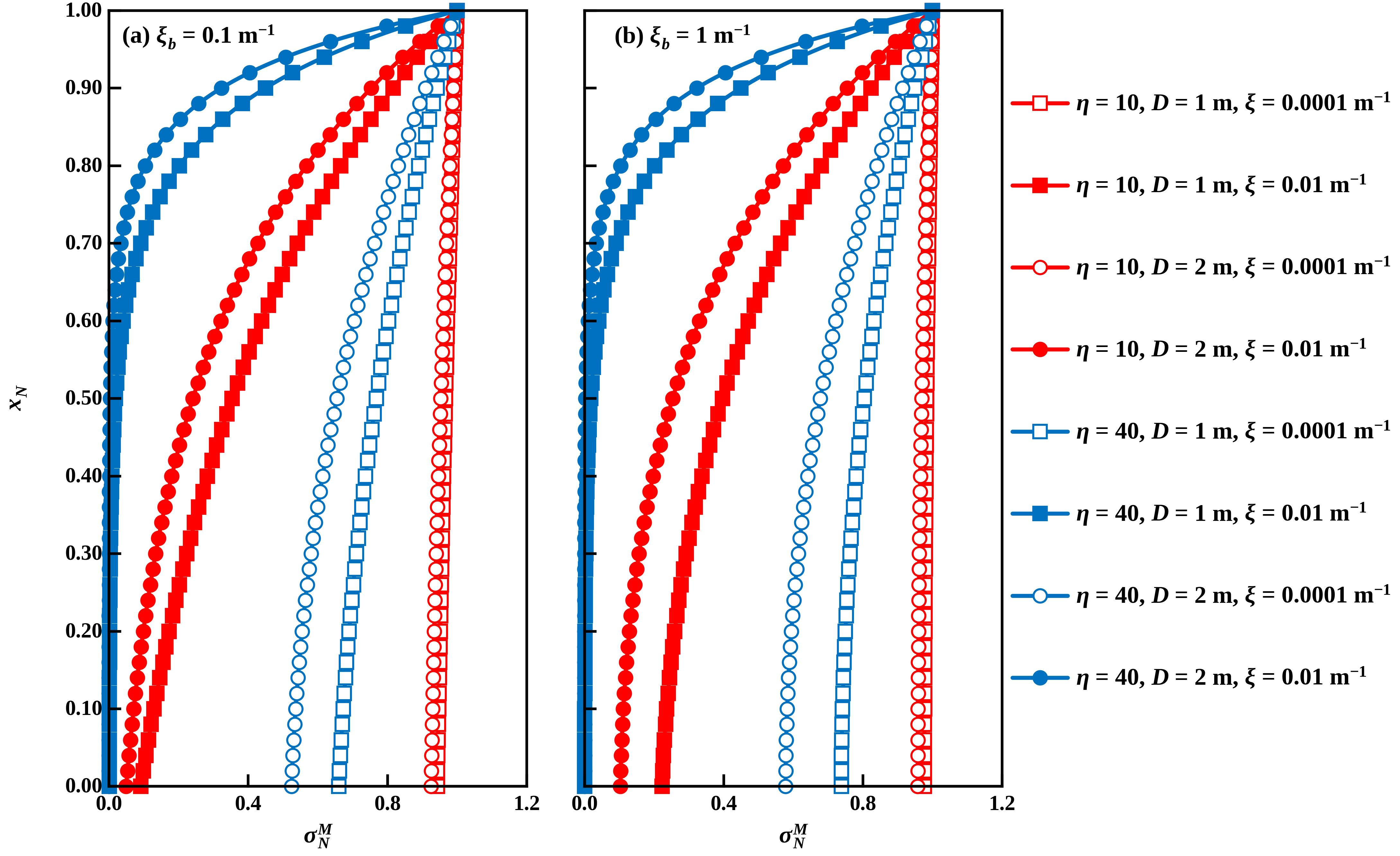
Figure 24.
Combined dimensionless displacement vs. dimensionless depth for semi-floating piles.
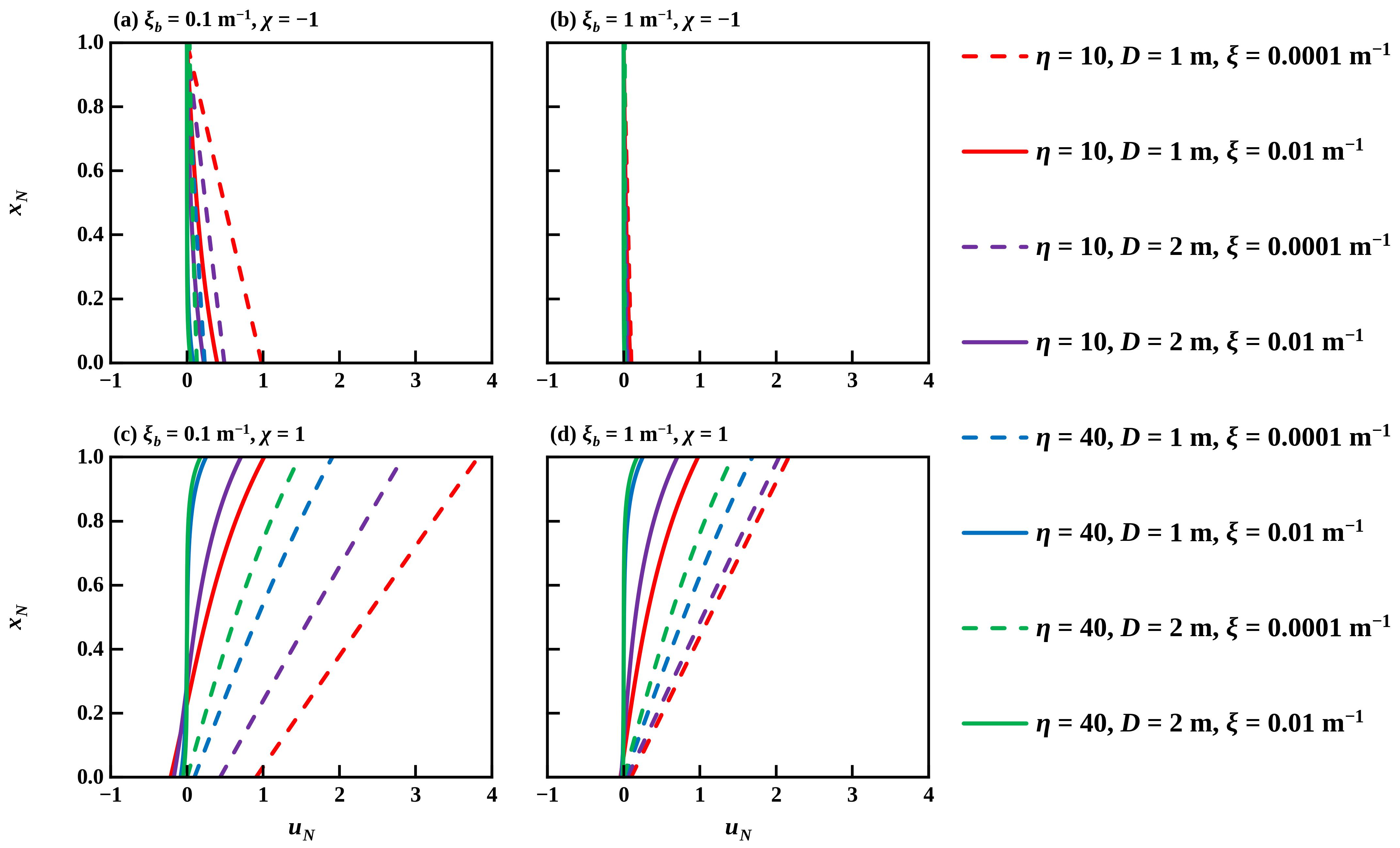
Figure 25.
Combined dimensionless stress vs. dimensionless depth for semi-floating piles.
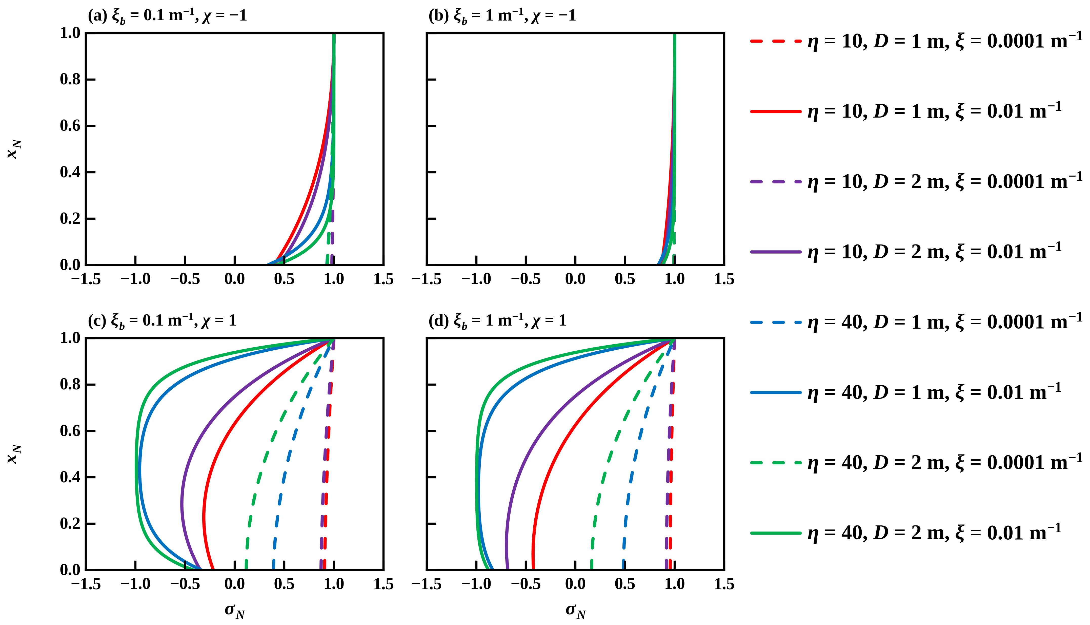
Figure 26.
Combined dimensionless displacement vs. dimensionless depth for all selected values of χ, for semi-floating piles with ξb = 0.1 m−1. Top row (heating), Bottom row (cooling).
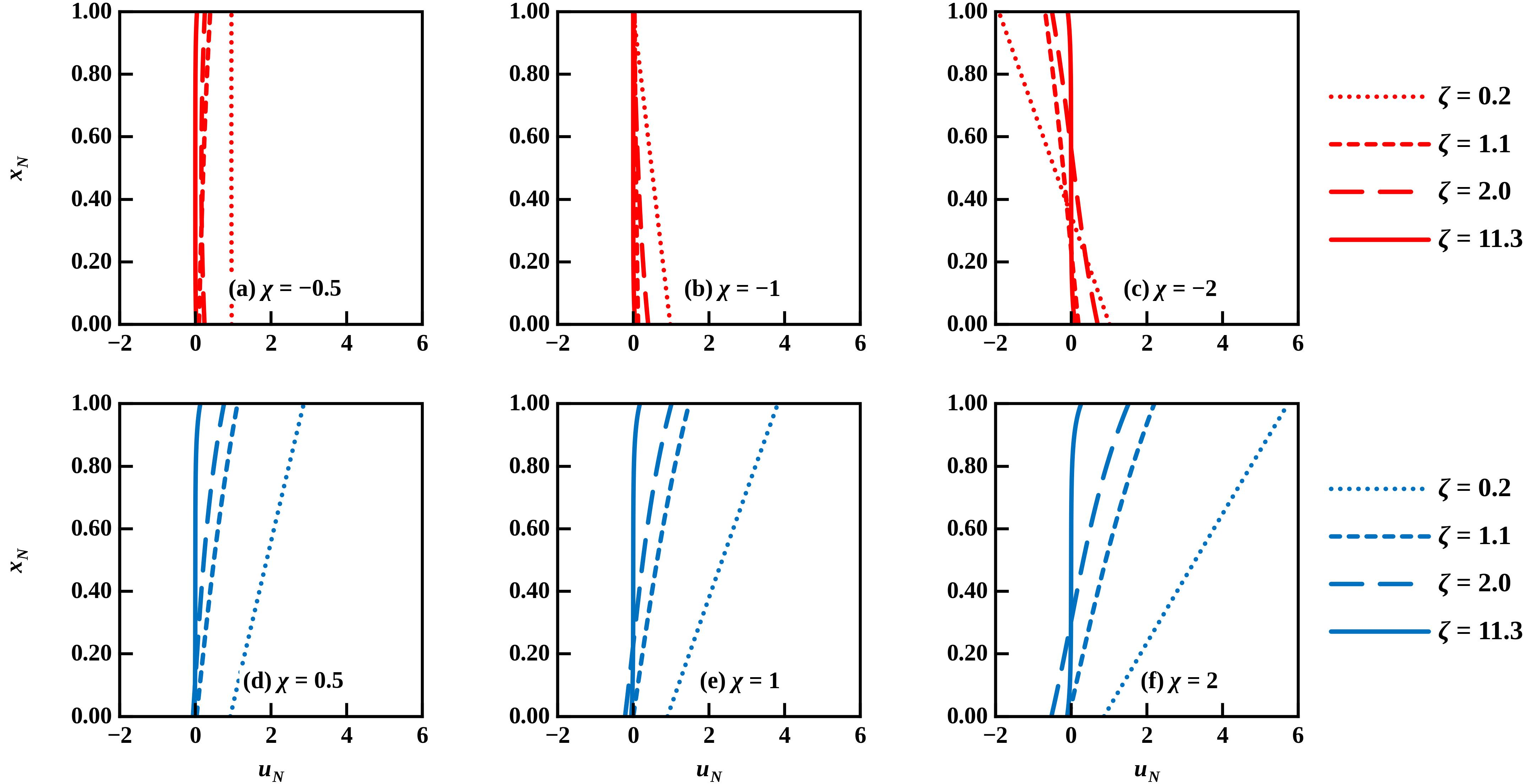
Figure 27.
Combined dimensionless stress vs. dimensionless depth for all selected values of χ, for semi-floating piles with ξb = 0.1 m−1. Top row (heating), Bottom row (cooling).
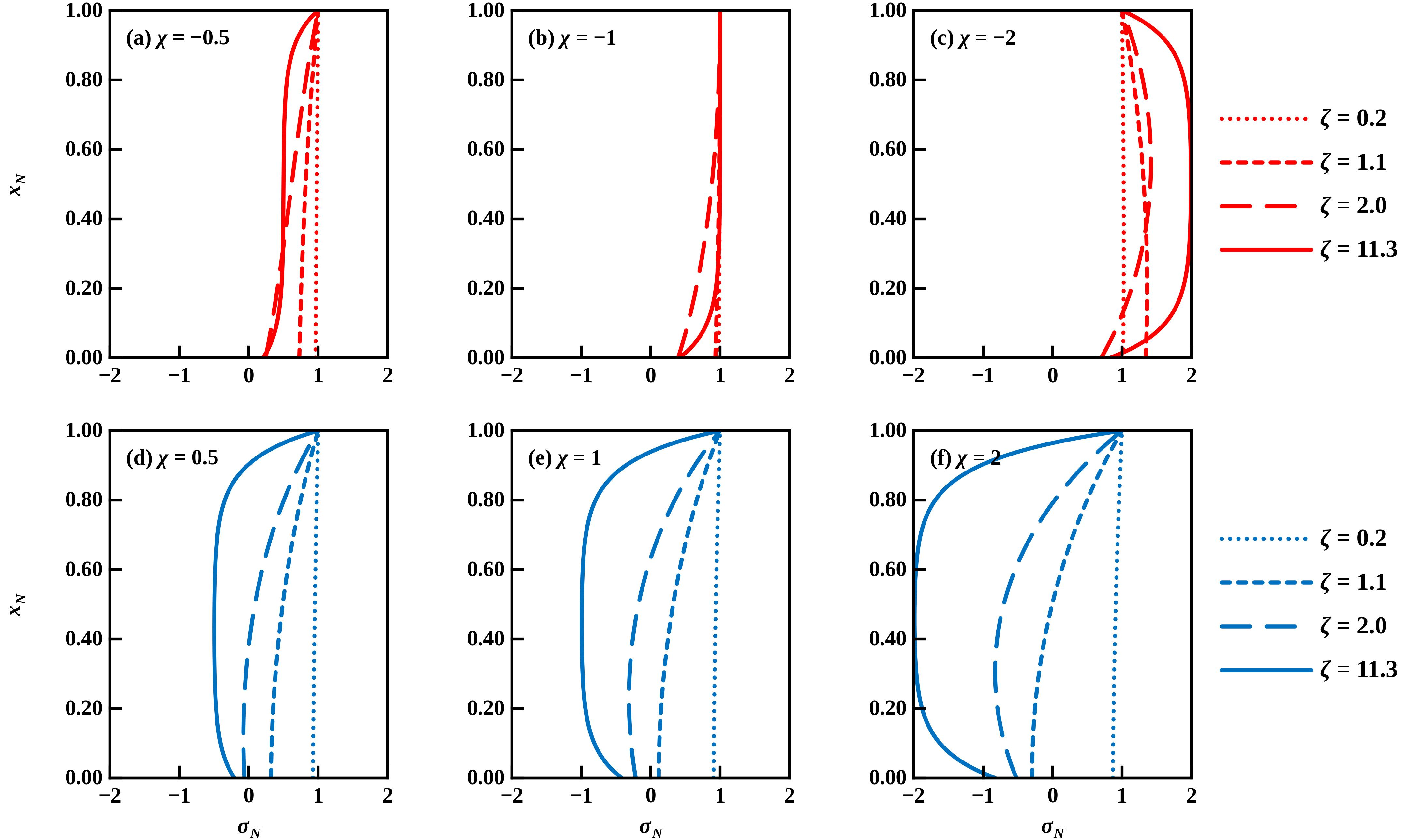
Figure 28.
Combined dimensionless displacement vs. dimensionless depth for all selected values of χ, for semi-floating piles with ξb = 1 m−1. Top row (heating), Bottom row (cooling).
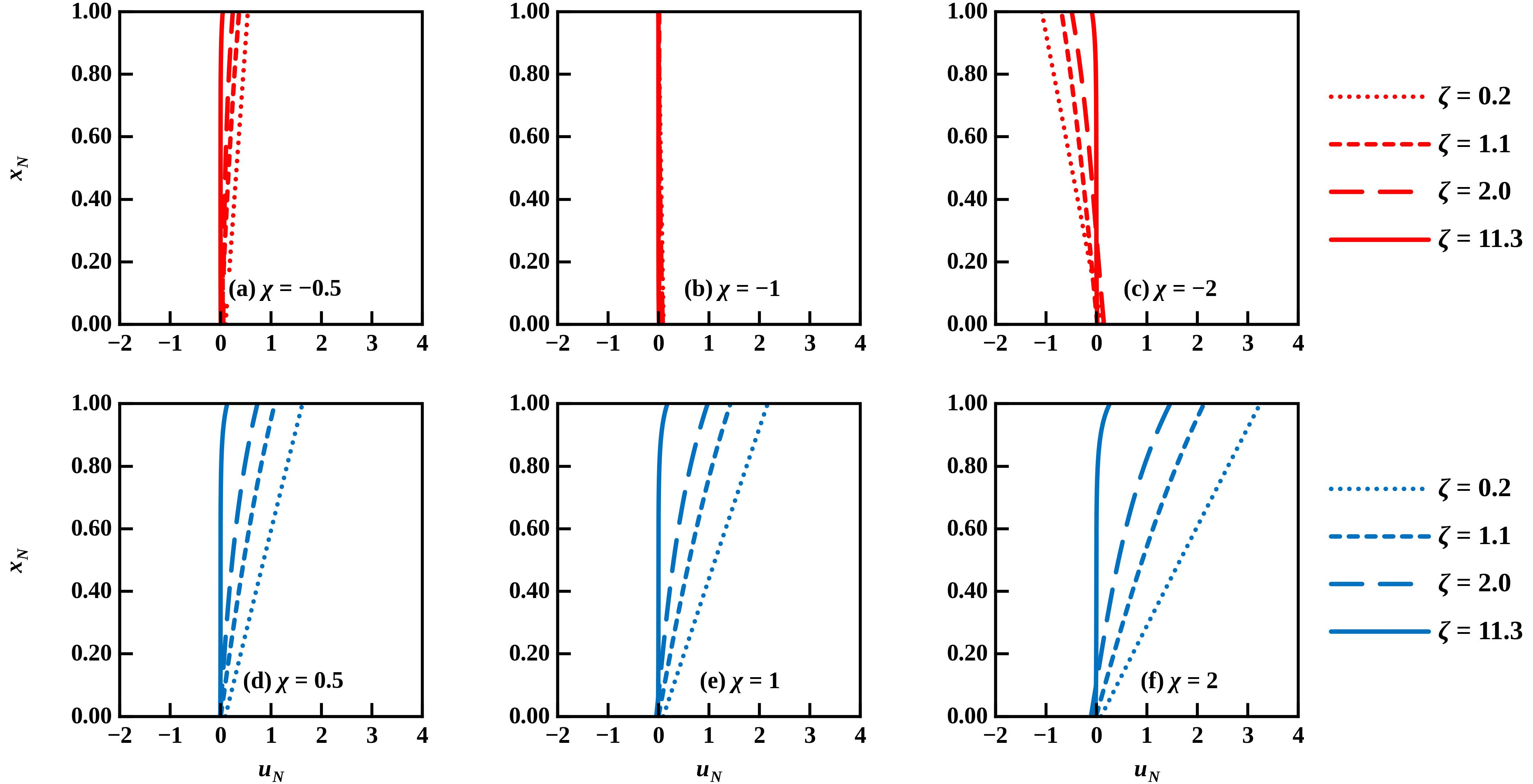
Figure 29.
Combined dimensionless stress vs. dimensionless depth for all selected values of χ, for semi-floating piles with ξb = 1 m−1. Top row (heating), Bottom row (cooling).
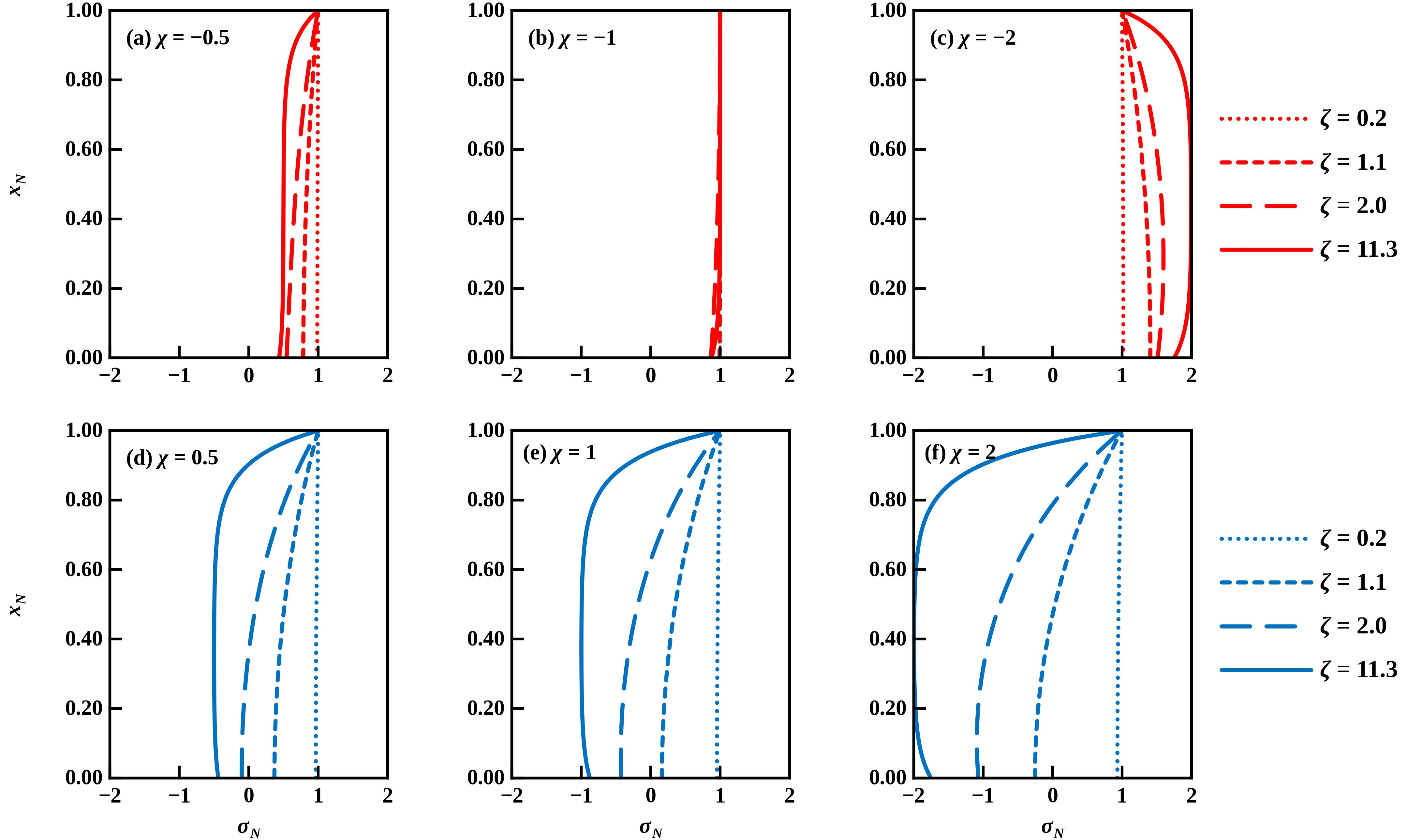
Figure 30.
Maximum dimensionless thermal displacement vs. ξ (m−1) for semi-floating piles.
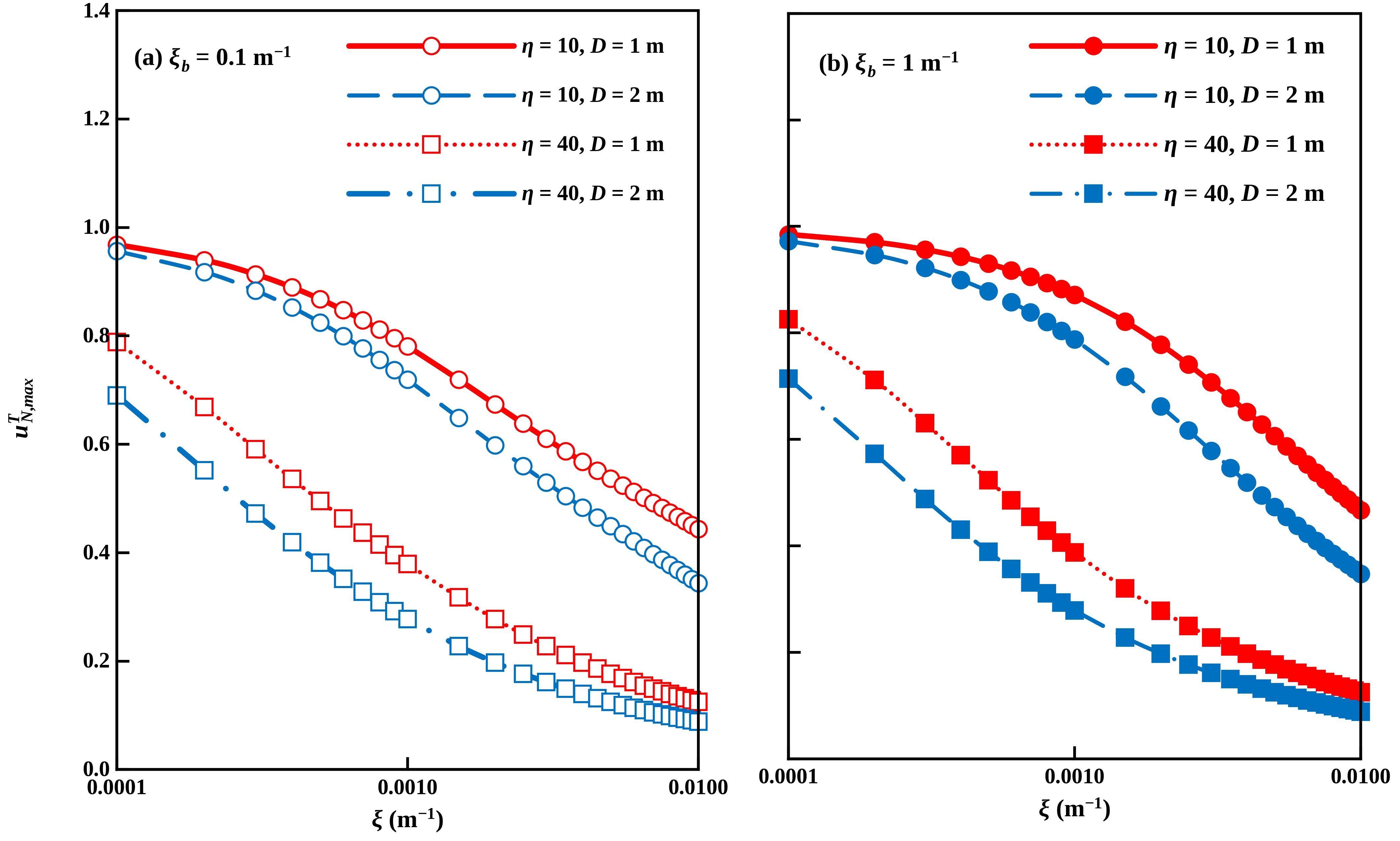
Figure 31.
Maximum dimensionless mechanical displacement vs. ξ (m−1) for semi-floating piles.
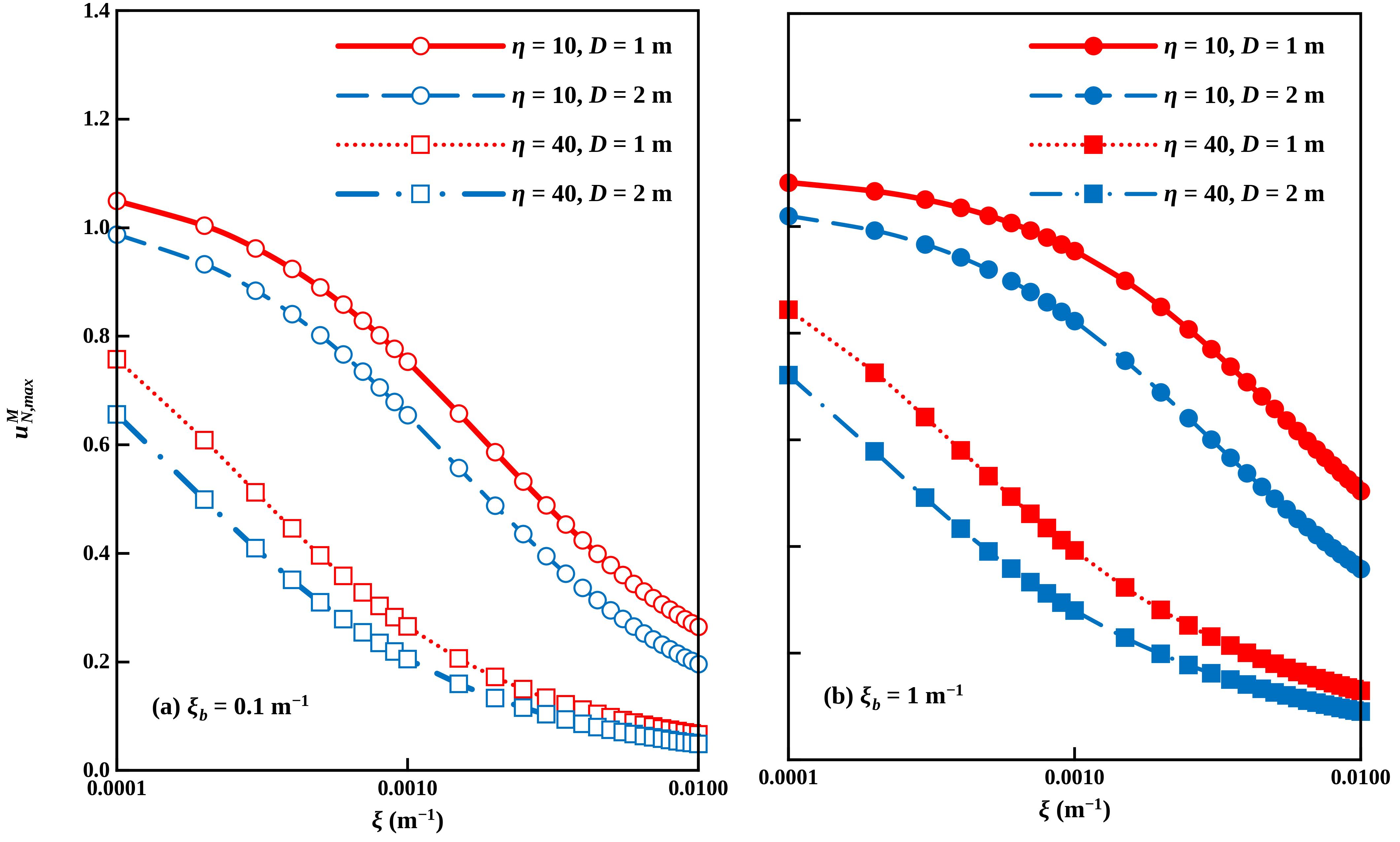
Figure 32.
Minimum dimensionless thermal stress vs. ξ (m−1) for semi-floating piles.
3.4. Practical Application
The normalized solutions can be used directly in the preliminary design of energy piles. This is demonstrated herein for an end-bearing pile subjected to cooling. Iβ = 1 for an end-bearing pile, and the maximum combined normalized displacement develops at the pile head, while the maximum combined normalized stress develops at the pile tip. Combinations of Equations (30) and (34) for displacement and Equations (31), (39), and (40) for stress result in:
where positive values correspond to the pile head settlement, and compressive normalized stress, respectively. The corresponding dimensional values are
During cooling (χ > 0), σmax,N decreases with increasing ζ and becomes negative for ζ > ζlim (ζlim = 0.962 for χ = 2). For ζ > ζlim, the end-bearing pile transforms into a fully floating pile under combined thermo-mechanical loading. The corresponding pile length (Lmax) can be obtained from Equation (23) as:
The design procedure for the preliminary selection of the pile length is summarized in Figure 33. It is based on Equations (43) and (44), which are plotted against ξ in Figure 34 and Figure 35 for D = 1 m, η = 10–40 and χ = 2, and consists of four steps: (1) the maximum length Lmax is obtained where the vertical line for the selected ξ crosses σmax,N = 0 in Figure 34 (or from Equation (46)); (2) trial lengths L ≤ Lmax are selected, and the corresponding σmax,N, i.e., the stress transmitted to the bearing stratum, is determined from Figure 34; (3) the corresponding umax,N is determined from Figure 35; and (4) umax is calculated from Equation (45) and compared with the allowable displacement uallow. The lengths that result in umax ≤ uallow are acceptable as preliminary pile lengths based on the elastic analysis.
Figure 33.
Procedure for the preliminary selection of the length of an end-bearing energy pile using the dimensionless design charts.
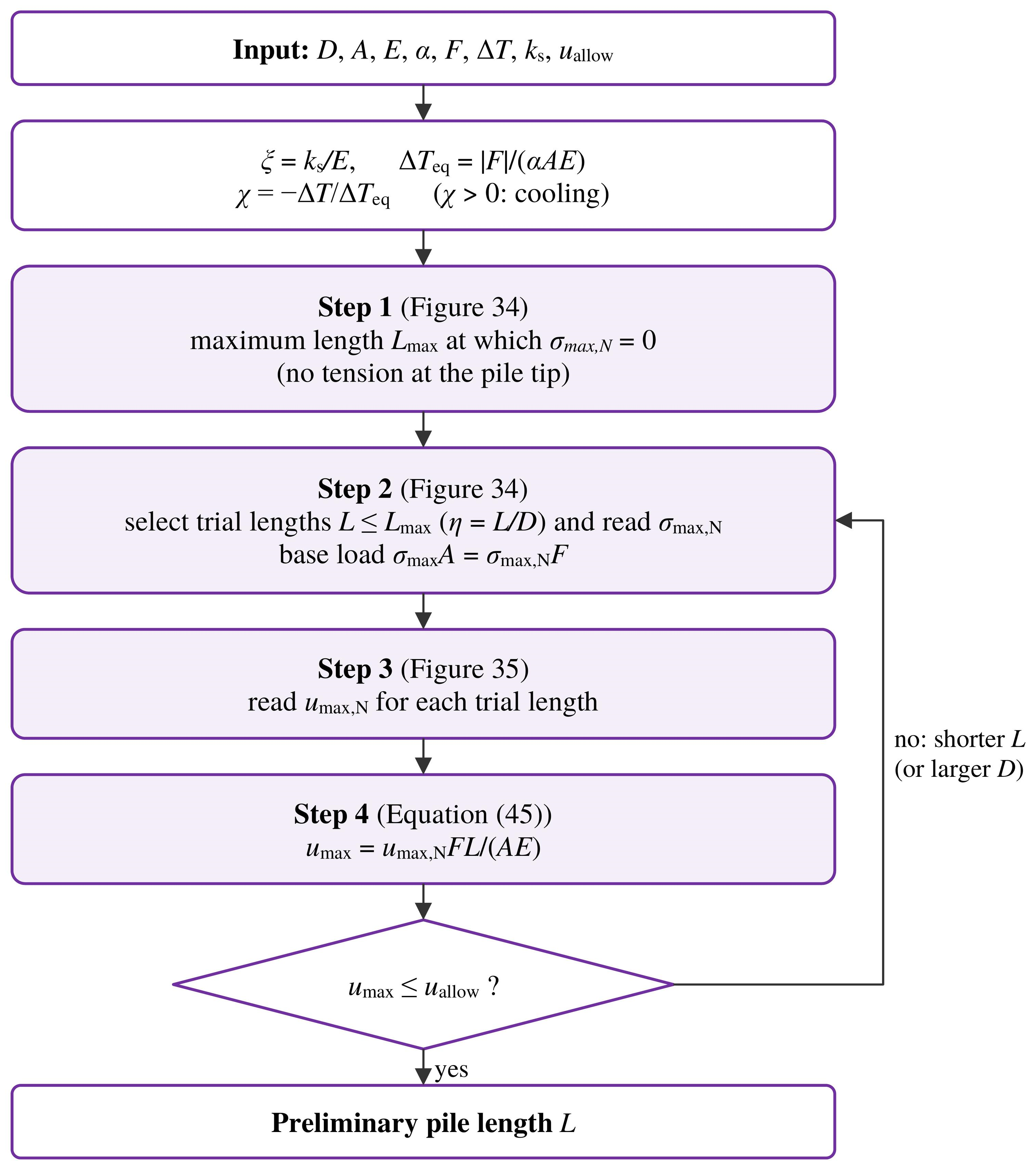
As an example, consider a concrete energy pile with D = 1 m (A = 0.785 m2), E = 30 GPa, and α = 1.0 × 10⁻⁵ °C−1, carrying a working load F = 1 MN in a soil with ξ = 2 × 10⁻⁴ m−1 (ks = 6 MN/m3) and an allowable displacement uallow = 5 mm. The allowable displacement is project-specific and follows from the serviceability limit states of the superstructure, which for energy piles include limits on differential displacement and angular distortion [14]. Because the thermally induced displacement is cyclic and develops only in the heat-exchanger piles, uallow = 5 mm is adopted here. This value corresponds to the relative rotation of 1/500, which is acceptable for many structures [15,16], over a spacing of 2.5 m (2.5D) between an energy pile and an adjacent conventional pile, and it is well below the total settlement of 50 mm that is often acceptable for normal structures [15]. Hence, ΔTeq = 4.2 °C, so that χ = 2 corresponds to cooling of the pile by 8.5 °C, F/(AE) = 4.25 × 10⁻⁵, and F/A = 1.27 MPa.
Step 1. The vertical line at ξ = 2 × 10⁻⁴ m−1 in Figure 34 crosses the zero-stress line between the curves for η = 30 and 40, giving Lmax ≈ 34 m (Equation (46): Lmax = 34.0 m). A 40 m long pile would develop toe tension (σmax,N = −0.25) and is therefore rejected.
Figure 34.
Combined stress at the pile tip, σN,max, vs. stiffness ratio ξ (m−1) for end-bearing piles (D = 1 m) during cooling (χ = 2); negative values denote tension. The red dashed lines show the worked example for ξ = 2 × 10⁻⁴ m−1; circles denote the trial lengths L = 10, 20, and 30 m; the diamond denotes the maximum length Lmax = 34 m (σmax,N = 0); and the square the rejected length L = 40 m.
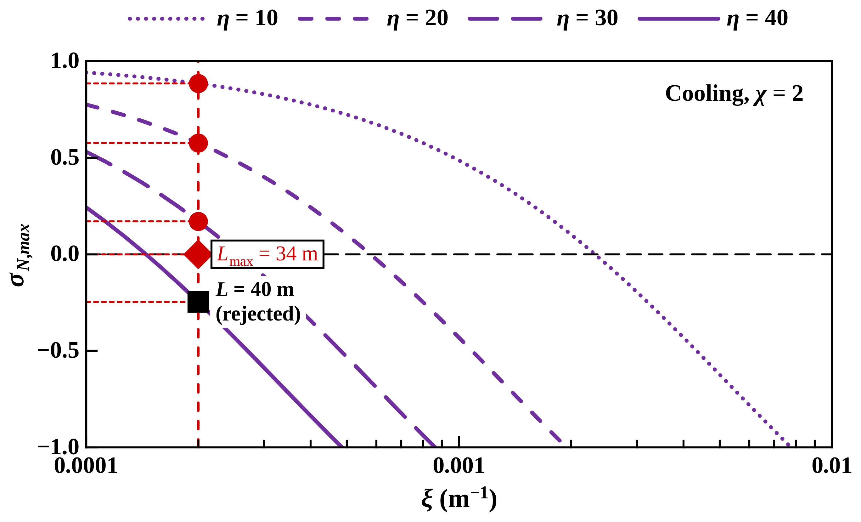
Step 2. Three trial lengths smaller than Lmax, i.e., L = 10, 20, and 30 m, are selected. Figure 34 gives corresponding σN,max = 0.88, 0.58, and 0.17 (horizontal lines), respectively, i.e., σmax = 1.13, 0.73, and 0.22 MPa, respectively, so that 88%, 58%, and 17% of the pile head stress or mechanical load applied at the pile head is transmitted to the bearing stratum.
Figure 35.
Maximum combined displacement, uN,max, vs. stiffness ratio ξ (m−1) for end-bearing piles (D = 1 m) during cooling (χ = 2). Symbols correspond to those in Figure 34.
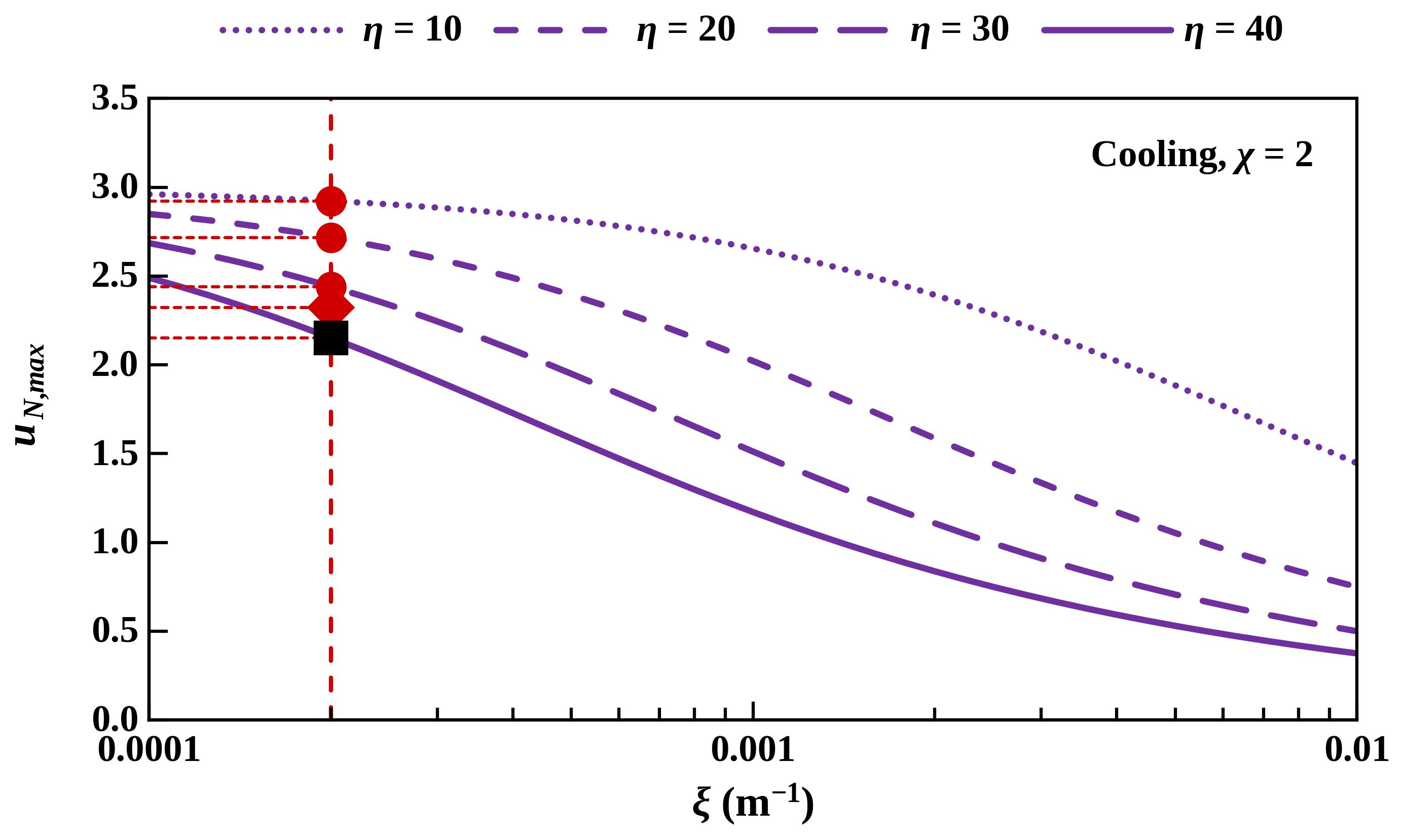
Step 4. Equation (45) gives umax = 1.24, 2.31, and 3.11 mm for L = 10, 20, and 30 m, respectively, and 3.36 mm at Lmax (Table 3).
All three trial lengths satisfy umax ≤ uallow = 5 mm. Displacement increases with pile length, while tip stress decreases. The tip stress is inherently small in this case due to cooling and tension limitation, and minimizing the displacement would be the primary concern. From a displacement perspective, the optimal length would be 10 m, which would also be economically efficient. However, this length would adversely affect the pile’s heat-exchange capacity, as it does not extend sufficiently into the undisturbed ground temperature zone. Thus, keeping in mind that this is an energy pile, the length of 20 m or 30 m would be a better choice, as both of these lengths satisfy the displacement limitation. The final length should be selected by considering the displacement limitation, heat exchange capacity and efficiency, and ultimate state, i.e., providing a sufficient safety margin against the bearing capacity failure of the soil.
It is interesting to compare the two pile lengths required for zero stress at the tip, corresponding to two different stiffness ratios (ξ). As explained above, for , the corresponding length is 34 m, while for example, for , the corresponding length is 10 m (Figure 34), both for a diameter of 1 m. According to Figure 35, corresponding pile head displacements would be 3.3 mm for L = 34 m and 1.0 mm for L = 10 m. Thus, the stiffer soil reaches zero tip stress at the smaller length, accompanied by a smaller pile head displacement, while the softer soil reaches zero tip stress at the larger length, accompanied by a larger pile head displacement, under combined mechanical loading and cooling.
It is emphasized that these estimates are based on the linear elastic response of a homogeneous soil layer, the thermo-elastic response of the pile, a rigid base or an end-bearing pile, and a uniform temperature change within the pile. The estimates are intended for preliminary design and must be complemented by checks of geotechnical capacity and code-based structural design.
4. Conclusions
A dimensionless form of the analytical solutions for displacement, strain, and stress in energy piles subjected to constant mechanical load and varying thermal loads, under different boundary conditions, has been derived, based on the elastic and thermo-elastic responses of the soil and pile, respectively.
- (1)
- The minimum number of composite parameters governing the response was determined based on the rigorous application of Buckingham Π theorem to be two, i.e., , and . Sensitivity analysis was subsequently conducted by plotting the normalized thermal, mechanical, and combined displacement and stress responses over a wide range of control parameters.
- (2)
- For the largest value of , the minimum value of normalized thermal stress is −1 for end-bearing, fully floating, and semi-floating piles. However, this value is reached at different locations along the pile due to different boundary conditions. In fully floating piles, it occurs around the mid-length, while in end-bearing piles, the minimum stress extends to the pile tip, and the minimum normalized thermal stress pattern in semi-floating piles falls between that of the end-bearing and fully floating piles. On the contrary, minimum normalized mechanical stress for the highest value of is equal to zero throughout a significant portion of the pile length for all boundary conditions because mechanical load is carried by the soil.
- (3)
- In case that thermal load is equal to equivalent thermal load (χ = −1), combined normalized displacement is by definition equal to zero at the pile head. However, in end-bearing piles this loading scenario results in the zero combined displacement throughout the pile length, while combined normalized stress is equal to 1 throughout the pile length, regardless of the value. In semi-floating and fully floating piles, the maximum combined normalized stress is also equal to 1 regardless of value but not throughout the pile length.
- (4)
- In the case of cooling (χ = 1), the minimum combined normalized stress is −1 at different locations along the pile depth for different boundary conditions.
- (5)
- Similarly, for the larger amount of heating and cooling (), the maximum magnitude of normalized combined stress is 2 for heating, and the minimum value is −2 for cooling. These extreme values are reached at different locations along the pile length for different boundary conditions.
- (6)
- Both thermal and mechanical loading produce small displacement in stiff soils, i.e., for large values.
- (7)
- For the smallest value , normalized mechanical stress is 1 along the pile length for end-bearing and semi-floating piles, while in fully floating piles, it ranges from 1 at the pile head to zero at the pile tip. Nevertheless, in this case, induced thermal stresses in the pile are very small across all boundary conditions, as thermal load is absorbed through the large magnitude of displacement.
- (8)
- The net pile head displacement is always larger in the case that mechanical load is combined with cooling and distribution of displacement along the pile length varies in accordance to different boundary conditions. Thus, for small shear stiffness of the soil, small tip stiffness displacements are large, and the energy pile response is flexible.
The actual soils will fall between these two extremes, generating a multifaceted solution space that became accessible through the formulation of the normalized analytical solutions. As illustrated herein, the response curves for the maximum magnitudes of combined normalized displacements and stresses can be used to evaluate different pile-length selections for a given soil stiffness and determine whether the corresponding displacements and stresses are acceptable in accordance with the design guidelines.
Author Contributions
Conceptualization, D.P.; methodology, C.D.B.A. and D.P.; software, C.D.B.A.; validation, C.D.B.A. and D.P.; formal analysis, C.D.B.A. and D.P.; investigation, C.D.B.A. and D.P.; writing—original draft preparation, D.P.; writing—review and editing, C.D.B.A. and D.P.; visualization, C.D.B.A. and D.P.; supervision, D.P. All authors have read and agreed to the published version of the manuscript.
Funding
This research received no external funding.
Data Availability Statement
The original contributions presented in this study are included in the article. Further inquiries can be directed to the corresponding author.
Acknowledgments
During the preparation of this manuscript, the authors used Grammarly (v1. 2.303.1975) for the purpose of correcting grammar and spelling. The authors have reviewed and edited the output and take full responsibility for the content of this publication.
Conflicts of Interest
The authors declare no conflicts of interest.
Notation
The following symbols are used in this manuscript:
| A | Cross-sectional area of the pile |
| ai, bi, ci | Exponents of the repeating variables in the Π group, Πi (Equation (18)) |
| cA, cp | Shape factors relating the cross-sectional area and perimeter to the pile diameter (A = cAD2, p = cpD) |
| C1, C2 | Integration constants (Equation (3)) |
| D | Pile diameter, or side length of a square cross-section |
| E | Elastic modulus of the pile |
| F | Axial force (mechanical load) applied at the pile head (kN) |
| f | Functions relating to the governing variables or the dimensionless groups (Equations (16), (22), (25), and (A28)) |
| Iβ | Thermal equivalence factor (Equation (28)); Iβ = 1 for an end-bearing pile |
| i | Index of the Π groups (i = 1 to 6; Equation (18)) |
| k | Number of independent dimensionless (Π) groups (Equation (15)) |
| kb | Stiffness of the soil-substituting normal spring at the pile tip |
| ks | Stiffness of the soil-substituting shear spring along the pile shaft |
| L | Pile length |
| Lmax | Maximum length of an end-bearing pile for which no tension develops at the pile tip during cooling (Equation (46)) |
| m | Rank of the dimensional matrix |
| n | Number of governing variables |
| p | Perimeter of the pile cross-section |
| Qi | Non-repeating variable used to form the Π group Πi |
| r | Thermal-load indicator (r = 1 for thermal and thermo-mechanical loading, r = 0 for mechanical loading; Equations (5)–(14) and (24)) |
| s | Mechanical-load indicator (s = 1 for mechanical and thermo-mechanical loading, s = 0 for thermal loading; Equations (7)–(14)) |
| u | Dimensional vertical displacement of the pile, positive upwards |
| uM, uT | Dimensional mechanical and thermal displacement of the pile |
| uallow | Allowable dimensional displacement at the pile head |
| umax | Maximum combined thermo-mechanical dimensional displacement at the pile head (Equation (45)) |
| uN | Dimensionless combined thermo-mechanical displacement (Equation (30)) |
| Sum of the dimensionless thermal and dimensionless mechanical displacements (Equations (24) and (26)) | |
| uNM, uNT | Dimensionless mechanical and thermal displacement (Equations (20) and (21)) |
| uN,max | Dimensionless maximum combined displacement at the pile head (Equation (43)) |
| x | Vertical coordinate originating at the pile tip and positive upwards |
| xN | Normalized vertical coordinate, x/L (Equation (19)) |
| α | Coefficient of thermal expansion of the pile (1/temperature unit) |
| β | Tip stiffness group, β = ηξbD = kbL/E (Equation (23)) |
| ΔT | Temperature change of the pile with respect to the surrounding soil, positive for heating (temperature unit) |
| ΔTeq | Equivalent temperature change, i.e., temperature change that produces zero combined displacement at the pile head (Equation (27)) (temperature unit) |
| ε | Axial strain in the pile |
| εM, εT | Mechanical and thermal axial strain in the pile |
| εf | Free thermal strain, αΔT (Equation (5)) |
| εσ | Stress-inducing strain (Equation (5)) |
| εNM, εNT | Normalized mechanical and thermal strain (Equations (20) and (21)) |
| ζ | Composite parameter, ζ = ψL = 2η(ξD)1/2 (Equation (23)) |
| ζlim | Value of ζ at which the combined stress at the pile tip becomes zero in end-bearing piles (Equation (46)) |
| η | Length-to-diameter ratio, L/D |
| Πi | Dimensionless (Π) groups (i = 1 to 6) |
| Π1,u, Π1,ε, Π1,σ | Π groups for displacement, strain, and stress (Table 1) |
| ξ | Ratio of the shear spring stiffness to the elastic modulus of the pile, ks/E |
| ξb | Ratio of the normal spring stiffness at the pile tip to the elastic modulus of the pile, kb/E |
| σ | Axial stress in the pile |
| σM, σT | Mechanical and thermal stress in the pile |
| σmax | Maximum combined thermo-mechanical stress at the pile tip (Equation (45)) |
| σN | Normalized combined thermo-mechanical stress (Equation (31)) |
| σNM, σNT | Normalized mechanical and thermal stress (Equations (20) and (21)) |
| σN,max | Normalized maximum combined stress at the pile tip (Equation (44)) |
| χ | Thermal load ratio, ΔT/ΔTeq (χ < 0 for heating and χ > 0 for cooling; Equation (29)) |
| ψ | Load-transfer parameter, ψ2 = (ks/E)(p/A) (Equation (2)) |
| Fundamental dimensions (Appendix A) | |
| M | Mass |
| L | Length |
| Tm | Time |
| T | Temperature |
Appendix A
This appendix gives the dimensions of the variables, the dimensional matrices, and the step-by-step derivation of the Π groups summarized in Section 2.2 and Table 1.
Appendix A.1. Dimensions of the Variables and Dimensional Matrices
The fundamental dimensions are mass (), length (), time (), and temperature (). Force is a derived quantity with the dimension (Newton’s second law), so that stress, elastic modulus, and spring stiffness are expressed in terms of , , and . The dimensions of the variables are listed in Table A1.
Table A1.
Dimensions of the variables in the ––– system.
The dimensional matrix for thermal loading is given in Table A2.
Table A2.
Dimensional matrix for thermal loading.
The row is equal to the row multiplied by , so the four rows are linearly dependent, and all determinants vanish. The rank of the matrix is the order of its largest non-vanishing determinant [9,10]. The sub-matrix formed by the rows , , and and the columns , , and has a non-zero determinant,
which gives the rank . The dimensional matrix for mechanical loading is given in Table A3.
Table A3.
Dimensional matrix for mechanical loading.
Again, the row is equal to the row multiplied by (including the column ), so all determinants vanish. The sub-matrix formed by the rows and and the columns and gives
so that the rank is .
Appendix A.2. Π Groups for Thermal Loading
With the repeating variables , , and , each Π group is formed with one of the remaining variables (Equation (18)). The exponents follow from the condition of dimensional homogeneity [10,11]
Equating the exponents of , , and T on both sides gives three linear equations for , and . The equation for is identical to the equation for because the row of the dimensional matrix depends on the row.
Π1 (displacement, ). With ,
and therefore
Π2 (location, ) and Π3 (diameter, ). The variables and have the same dimension as , so , , and . This gives and ; the inverse of , which is also dimensionless, was used for Π3:
Π4 (soil stiffness, ). With ,
and therefore
Π5 (pile tip soil stiffness, ). Since has the same dimension as , , , and :
Π6 (thermal expansion coefficient, ). With ,
and therefore
Other dependent variables ( and ). Replacing with and leaves Π2 to Π6 unchanged. For the strain, which is dimensionless,
For the stress, with ,
and therefore
Appendix A.3. Π Groups for Mechanical Loading
With the repeating variables and , each Π group is formed with one of the remaining variables :
Equating the exponents of and gives two equations for and ; the equation for is again identical to the equation for .
Π1 (displacement, ). With ,
and therefore
Π2 (location, ) and Π3 (diameter, ). As for thermal loading, and :
Π4 (soil stiffness, ). With ,
and therefore
Π5 (pile tip soil stiffness, ). Since has the same dimension as , , and :
Π6 (applied load, ). With ,
and therefore
Other dependent variables ( and ). Replacing with and leaves Π2 to Π6 unchanged. For the strain,
and for the stress,
and therefore
Appendix A.4. Normalized Solutions and Composite Groups
By Rule 2, the functions are proportional to , which is taken out as a factor, for example, for the displacement
For mechanical loading, the cross-sectional area enters through , a Π group multiplied by a constant ( for circular and for square piles). The normalized mechanical solutions in Equation (21) are then obtained as
The stiffness groups are related to , , and by
and, with for circular and square piles, the composite parameters and are given by:
References
- Cossel, A.E. Analytical Solutions for Thermo-Mechanical Soil Structure Interaction in Energy Piles. Master’s Thesis, Kansas State University, Manhattan, KS, USA, 2019. Available online: https://krex.k-state.edu/items/6feb9d97-a467-4f73-9555-186043b85921 (accessed on 1 October 2026).
- Iodice, C.; Di Laora, R.; Mandolini, A. Analytical solutions for ultimate limit state design of thermal piles. J. Geotech. Geoenviron. Eng. 2020, 146, 04020016. [Google Scholar] [CrossRef] [Scilit]
- Perić, D.; Cossel, A.E.; Sarna, S.A. Analytical solutions for thermomechanical soil structure interaction in end-bearing energy piles. J. Geotech. Geoenviron. Eng. 2020, 146, 04020047. [Google Scholar] [CrossRef] [Scilit]
- Saeidi Rashk Olia, A.; Cossel, A.E.; Perić, D. Analytical solutions for thermomechanical soil–structure interaction in single semifloating energy piles embedded in a layered soil profile. J. Geotech. Geoenviron. Eng. 2022, 148, 04022080. [Google Scholar] [CrossRef] [Scilit]
- Olia, A.S.R.; Perić, D. Thermomechanical soil–structure interaction in single energy piles exhibiting reversible interface behavior. Int. J. Geomech. 2021, 21, 04021065. [Google Scholar] [CrossRef] [Scilit]
- Saeidi Rashk Olia, A.; Perić, D. Analytical solutions for thermomechanical soil structure interaction in single energy piles exhibiting irreversible interface behavior. Int. J. Geomech. 2023, 23, 04023234. [Google Scholar] [CrossRef] [Scilit]
- Buckingham, E. On physically similar systems; illustrations of the use of dimensional equations. Phys. Rev. 1914, 4, 345–376. [Google Scholar] [CrossRef] [Scilit]
- Bridgman, P.W. Dimensional Analysis; Yale University Press: New Haven, CT, USA, 1922. [Google Scholar]
- Langhaar, H.L. Dimensional Analysis and Theory of Models; John Wiley & Sons: New York, NY, USA, 1951. [Google Scholar]
- Szirtes, T. Applied Dimensional Analysis and Modeling, 2nd ed.; Butterworth-Heinemann: Burlington, MA, USA, 2007. [Google Scholar]
- White, F.M. Fluid Mechanics, 7th ed.; McGraw-Hill: New York, NY, USA, 2011. [Google Scholar]
- Birkhoff, G. Hydrodynamics: A Study in Logic, Fact, and Similitude, 2nd ed.; Princeton University Press: Princeton, NJ, USA, 1960. [Google Scholar]
- Barenblatt, G.I. Scaling, Self-Similarity, and Intermediate Asymptotics; Cambridge University Press: Cambridge, UK, 1996. [Google Scholar] [CrossRef] [Scilit]
- Rotta Loria, A.F. Performance-based design of energy pile foundations. DFI J. 2018, 12, 94–107. [Google Scholar] [CrossRef] [Scilit]
- EN 1997-1:2004; Eurocode 7: Geotechnical Design—Part 1: General Rules. European Committee for Standardization (CEN): Brussels, Belgium, 2004.
- Skempton, A.W.; MacDonald, D.H. The allowable settlements of buildings. Proc. Inst. Civ. Eng. 1956, 5, 727–768. [Google Scholar] [CrossRef] [Scilit]

Disclaimer/Publisher’s Note: The statements, opinions and data contained in all publications are solely those of the individual author(s) and contributor(s) and not of MDPI and/or the editor(s). MDPI and/or the editor(s) disclaim responsibility for any injury to people or property resulting from any ideas, methods, instructions or products referred to in the content. |
© 2026 by the authors. Licensee MDPI, Basel, Switzerland. This article is an open access article distributed under the terms and conditions of the Creative Commons Attribution (CC BY) license.