Performance Evaluation and Hybrid Combination of Modern Metaheuristics for the Optimal Design of Electromagnetic Devices

Abstract

Recent advancements in computational hardware and parallel processing are driving developments in metaheuristic algorithms. These advancements help solve increasingly complex real-world optimization problems. As a result, more sophisticated and computationally demanding algorithms can now be implemented. This paper presents a comparative performance evaluation of ten modern metaheuristic algorithms for the optimal design of Electromagnetic Devices (EMDs). It also evaluates seven well-established metaheuristics, which are referred to as reference algorithms. In addition to the comparison, a novel hybrid optimization strategy called Multiple Combined Algorithms for Optimization (MuCAO) is proposed. MuCAO probabilistically combines the best-performing algorithms to leverage their complementary strengths. All algorithms, including MuCAO, were tested on six benchmark problems with various complexities and design variables. These benchmarks include analytical models and problems based on the Finite Element Method (FEM). For validation, the approach was also applied to a real-life application, which is Sidelobe Level Reduction in a Circular Antenna Array (CAA). The results show that MuCAO outperformed all other algorithms and achieved the highest overall ranking. Three modern metaheuristics followed. The best-performing reference algorithm ranked lower, with DE in fifth place. The study confirms that modern metaheuristics generally offer superior performance for EMD design and optimization compared to traditional metaheuristics.

1. Introduction

Metaheuristics are stochastic optimization algorithms inspired by natural or physical phenomena. They aim to iteratively improve a set of solutions through mechanisms and approaches that balance exploration (searching new regions of the search space) and exploitation (refining promising regions of the search space) [1]. They can achieve satisfactory results for complex optimization problems in different areas, as reported by many authors in the literature [2,3,4].

The optimal design of Electromagnetic Devices (EMDs) using metaheuristic algorithms has been actively investigated over the last few decades. Numerous studies in the literature have employed both analytical models and Finite Element Models (FEMs) to solve various design problems [3,5,6,7]. The application of metaheuristics to EMD design can be traced back to the early 1990s. For instance, Reference [8] applied the Genetic Algorithm (GA) to optimize the magnetizer problem using a FEM-based model. Similarly, Reference [9] utilized Tabu Search (TS) to design a system of solenoids aimed at generating a highly homogeneous magnetic field within a defined region, also employing FEM simulations.

Reference [10] introduced the Intelligent Particle Swarm Optimization (IPSO) algorithm for optimizing the Loney problem based on an analytical model. The term “intelligent” was used to reflect the algorithm’s ability to observe particle behavior, learn from their experiences, and adopt a more informed movement strategy. Reference [11] employed a real-coded Clonal Selection Algorithm (RCSA) to solve the TEAM 22 benchmark problem using FEM. Moreover, Reference [12] improved the classical Simulated Annealing (SA) algorithm by introducing a restart mechanism to escape local minima. Their method was applied to both the TEAM 22 benchmark and a magnetic channel bar, using FEM simulations. Similarly, Reference [13] combined PSO with normative knowledge to optimize the Loney problem based on an analytical model. Reference [14] proposed an Improved Artificial Bee Colony (ABC) algorithm, OOABC, which incorporated two mechanisms to accelerate convergence. This approach was applied to the TEAM 22 problem and a loudspeaker problem, both modeled with FEM. Reference [15] applied the Black Hole-Based Optimization (BHBO) algorithm to the magnetizer problem using FEM. The same problem was also studied in [16] using the Electromagnetism-Like Mechanism (EM). Reference [17] introduced the Bacterial Chemotaxis Shape Optimizer (BCSO) for optimizing the electrode and electron gun problems, both using FEM-based approaches. Another work [18] proposed an Improved Teaching–Learning-Based Optimization (ITLBO) algorithm for the BLDC motor problem (analytical model) and the TEAM 22 benchmark (FEM). Similarly, Reference [19], applied the Modified Social Spider Optimization (MSSO) algorithm to optimize the Loney and BLDC problems using analytical models. A different work [20] used the Firefly Algorithm (FFA) to solve the electromagnetic shielding/shunting problem using FEM. A Wind-Driven Optimization (WDO) technique to address the TEAM 22 benchmark under interval uncertainty was introduced in [21]. The League Championship Algorithm (LCA) was also adopted in [22] to optimize the magnetizer and an outrunner-type BLDC motor. Furthermore, Reference [23] developed a robust-oriented Quantum-Inspired Evolutionary Algorithm (QEA) for the TEAM 22 benchmark, also under interval uncertainty, A modified Ant Colony Optimization variant (ACOR) for the Loney and TEAM 22 benchmarks was proposed in [24]. Finally, Reference [25] applied PSO to optimize a solenoid actuator by combining two objective functions into a single one to ensure higher and more consistent magnetic force within the effective working region.

The emergence of numerous high-performance metaheuristics was partly fueled by advances in computational power and algorithmic design. Hence, these metaheuristic methods are continually becoming more competitive, as noted by various authors. However, in the context of EMDs design, there is still a noticeable gap in the literature. Therefore, there is a need for comprehensive comparisons of modern metaheuristics applied to EMD design. To the best of the authors’ knowledge, only a limited number of studies have addressed this need [26].

For example, in [27], five metaheuristic algorithms, ACO, Biogeography-Based Optimization (BBO), Differential Evolution (DE), Population-Based Incremental Learning (PBIL), and Stud Genetic Algorithm (SGA), were applied and compared for the design and optimization of a planar array and an elliptical reflectarray. Another study [28] compared gradient-based and gradient-free optimization techniques for EMD design problems using FEM, where GA was employed as the representative metaheuristic, applied to TEAM 22 and TEAM 25 benchmarks.

Building on this foundation, the present work has two main objectives. The first is to provide a comprehensive and fair performance evaluation of ten recently developed metaheuristic algorithms for the optimal design of EMDs. To achieve this, the tested methods are assessed on six benchmark problems of different characteristics and are compared with seven well-established metaheuristics, thereby offering a broad comparative analysis across analytical and FEM-based design problems.

The second objective is to introduce a new adaptive hybrid optimization framework, referred to as MuCAO. Unlike a static hybrid approach or a simple sequential selection mechanism, MuCAO is designed as a performance-driven cooperative framework in which several metaheuristics with complementary search characteristics are combined using an adaptive probabilistic selection rule. The key idea is not merely to switch between algorithms but to continuously regulate their contribution according to two distinct and complementary indicators: their average historical performance and their best-achieved performance. This way, MuCAO promotes a dynamic balance between exploration and exploitation. This dual evaluation mechanism constitutes the main methodological insight of the proposed framework.

Accordingly, the main contributions of this paper can be summarized as follows:

• A comprehensive comparative assessment of ten modern metaheuristic algorithms against seven widely used reference methods for the optimal design of EMDs using six representative benchmark problems;
• The development of MuCAO, an adaptive multi-algorithm cooperation framework that combines multiple optimizers through a probabilistic selection mechanism guided jointly by average and best historical performance;
• The introduction of a flexible hybridization strategy that exploits the complementary strengths of different metaheuristics while reducing the risk of relying on a single optimizer across problems of different nature;
• Additional validation and sensitivity analyses to examine the influence of the weighting factors and the number of constituent algorithms on the behavior and performance of the proposed hybrid framework.

The remainder of this paper is organized as follows: Section 2 presents the metaheuristic algorithms evaluated in this study. Section 3 describes the selected benchmark problems used for algorithm testing. Section 4 provides the comparison and performance evaluation procedure, whereas Section 5 presents and discusses the results. Finally, Section 6 concludes the paper with a summary of key findings and future research directions.

2. Tested and Reference Metaheuristics

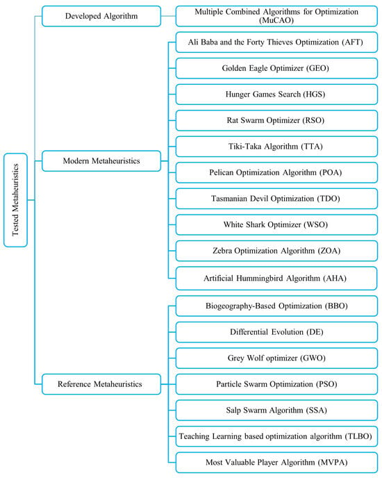
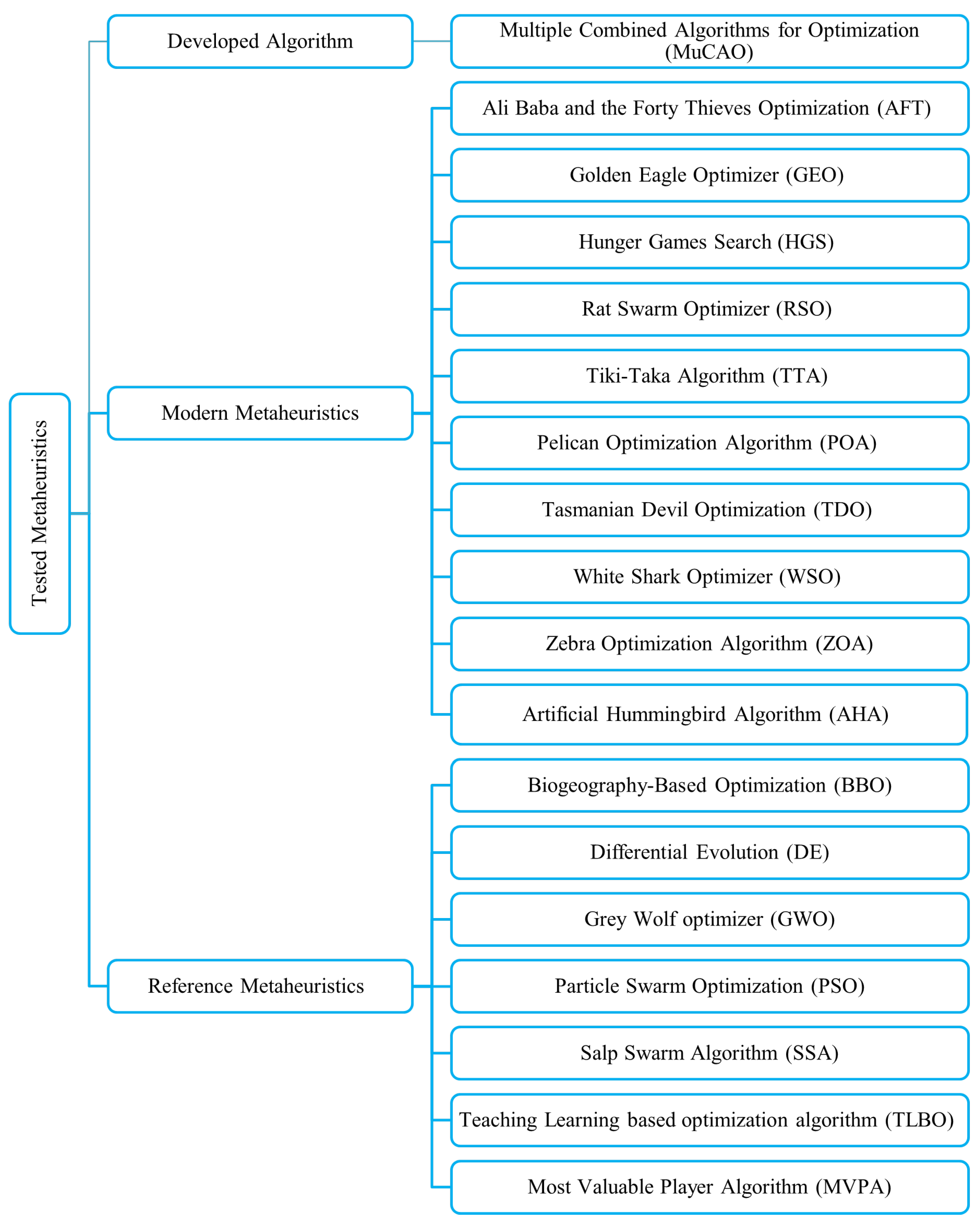
In this section, ten modern or recently developed metaheuristic algorithms are briefly discussed. Additionally, a novel hybrid approach, denoted MuCAO, is introduced. As highlighted earlier, MuCAO aims to combine the strengths of multiple algorithms into a single, more robust optimization strategy. Finally, to enable a meaningful performance comparison, seven well-known and widely used metaheuristics, referred to in this study as reference algorithms, are also included in the discussion in this section. The algorithms used in this study are shown in Figure 1.

Figure 1. Selected metaheuristics for comparison.

2.1. Modern Metaheuristics

The selected algorithms are briefly described below.

2.1.1. Ali Baba and the Forty Thieves Optimization (AFT)

The AFT algorithm, developed in 2021, is inspired by the famous tale of Ali Baba and the Forty Thieves. The authors used the clever strategies employed by the thieves to find Ali Baba, as well as the intelligent tactics used by Ali Baba’s maid to save him, as the basis for developing the AFT [29].

2.1.2. Golden Eagle Optimizer (GEO)

The GEO algorithm, developed in 2021, is inspired by the golden eagle’s hunting behavior. Eagles use a spiral trajectory to search for prey, transitioning smoothly from cruising to attacking. They balance exploration (searching for prey) and exploitation (attacking), adjusting their strategies based on energy efficiency and prey quality [30].

2.1.3. Hunger Games Search (HGS)

The HGS algorithm, also developed in 2021, is inspired by animals’ competitive behaviors driven by hunger. It models the decision-making process animals undergo in their search for food, balancing exploration, defense, and competition to ensure survival [31].

2.1.4. Rat Swarm Optimizer (RSO)

The RSO algorithm, developed in 2021, is inspired by the chasing and fighting behaviors of rats. Rats are socially intelligent and territorial animals, exhibiting aggressive behavior when competing for resources [32].

2.1.5. Tiki-Taka Algorithm (TTA)

The TA algorithm, developed in 2021, is inspired by the tiki-taka football style, known for its short passing, precise player positioning, and control of possession. Just as in tiki-taka, where players work together fluidly to build attacks, the TA emphasizes strategic movements and coordination to optimize the problem in hand [33].

2.1.6. Pelican Optimization Algorithm (POA)

The POA algorithm, developed in 2022, is inspired by the natural hunting behavior of pelicans, where the search agents are pelicans that are actively searching for food sources [34].

2.1.7. Tasmanian Devil Optimization (TDO)

The TDO algorithm, developed in 2022, is inspired by the natural feeding behavior of the Tasmanian devil. It mimics two primary feeding strategies of the Tasmanian devil: one where it feeds on carrion (dead animals) when available, and another where it actively hunts and attacks live prey [35].

2.1.8. White Shark Optimizer (WSO)

The WSO algorithm, developed in 2022, is inspired by the dynamic hunting behavior and unique sensory abilities of white sharks. Specifically, the WSO is inspired by the sharks’ method of ambush hunting, their streamlined swimming capabilities, and their keen senses of hearing and smell, which they use to detect prey from a distance [29].

2.1.9. Zebra Optimization Algorithm (ZOA)

The ZOA algorithm, developed in 2022, is inspired by the natural behaviors of zebras. The algorithm focuses on their foraging strategy, where a pioneer zebra guides the herd to food sources, and their defense strategy, where they escape predators in a zigzag pattern to confuse them [36].

2.1.10. Artificial Hummingbird Algorithm (AHA)

The AHA algorithm, developed in 2022, is inspired by the hummingbird’s flight abilities, memory, and foraging strategies. Their exceptional memory allows them to efficiently locate food sources, while their unique flight skills, including hovering and precise movement in any direction, are key elements in developing the algorithm [37].

2.2. Multiple Combined Algorithms for Optimization (MuCAO)

As mentioned earlier, in addition to evaluating the performance of several recently developed metaheuristics, this paper introduces a novel adaptive multi-algorithm optimization framework, denoted as MuCAO, in which multiple optimization algorithms with different search characteristics are cooperatively exploited. The motivation for this contribution arises from the well-known No Free Lunch (NFL) theorem, which states that no single optimization algorithm can be expected to perform best over all optimization problems. Accordingly, combining several algorithms with complementary strengths may provide a more robust and generalized optimization mechanism. The pseudoscope for MuCAO is given in Algorithm 1.

Algorithm 1: Pseudocode of the proposed MuCAO framework.

Input: Objective function $f\left(\mathbf{x}\right)$, candidate algorithm set $\mathcal{A}=\{A_1,A_2,\dots ,A_N\}$, number of runs R, population size $NP$, maximum number of iterations $T_{max}$, and maximum number of function evaluations $FE{S}_{max}$. Output: Optimization results.

1: Determine the lower and upper bounds, $\mathbf{LB}$ and $\mathbf{UB}$, and set the problem dimension $D\leftarrow \left|\mathbf{UB}\right|$. 2: Initialize $p_i\leftarrow 1/N$, $H_i\leftarrow \varnothing$, ${\overline{f}}_i\leftarrow 0$, $f_i^{\mathrm{best}}\leftarrow +\infty$, and $c_i\leftarrow 0$, for $i=1,2,\dots ,N$. 3: For $r=1$ to R, do:

3.1: If $p_1=p_2=\dots =p_N$, select $A_s$ uniformly at random; otherwise, select $A_s$ according to the probability vector $\mathbf{P}$.

3.2: Execute $A_s$ and obtain the fitness value $f^{\left(r\right)}$.

3.3: Update $H_s\leftarrow H_s\cup \left\{f^{\left(r\right)}\right\}$ and $c_s\leftarrow c_s+1$.

3.4: Update ${\overline{f}}_s\leftarrow \mathrm{mean}\left(H_s\right)$ and $f_s^{\mathrm{best}}\leftarrow min(f_s^{\mathrm{best}},f^{\left(r\right)})$.

3.5: For $i=1$ to N, compute: $$S_i^{\mathrm{avg}}\leftarrow \underset{j}{max}\left({\overline{f}}_j\right)-{\overline{f}}_i+\delta ,$$ $$S_i^{\mathrm{best}}\leftarrow \underset{j}{max}\left(f_j^{\mathrm{best}}\right)-f_i^{\mathrm{best}}+\delta ,$$ $$S_i\leftarrow w_1{S}_i^{\mathrm{avg}}+w_2{S}_i^{\mathrm{best}}.$$

If $S_i$ is undefined or $S_i<0$, set $S_i\leftarrow 0$.

3.6: Compute $S_{\mathrm{tot}}\leftarrow {\sum }_{i=1}^N{S}_i$.

3.7: If $S_{\mathrm{tot}}=0$, set $p_i\leftarrow 1/N$ for all $i=1,2,\dots ,N$; otherwise, set $$p_i\leftarrow {\displaystyle \frac{S_i}{S_{\mathrm{tot}}}}, i=1,2,\dots ,N.$$

4: Return the optimization results.

In the proposed framework, a pool of N candidate optimization algorithms is available for solving a given problem. Instead of assigning the same computational budget to all algorithms or relying on a single fixed optimizer, MuCAO adopts an adaptive selection mechanism in which one algorithm is selected at each run according to its historical performance. This strategy is intended to preserve a balance between exploration, by allowing all algorithms to be sampled, and exploitation, by increasingly favoring those that exhibit superior performance.

Initially, each algorithm $A_i$, where $i\in \{1,2,\dots ,N\}$, is assigned the same probability of selection:

$$p_i^{\left(0\right)}={\displaystyle \frac{1}{N}},\hspace{1em}\hspace{1em}i=1,2,\dots ,N.$$

(1)

After each run, the performance of the selected algorithm is recorded and used to update two main indicators for each algorithm $A_i$:

• The average fitness, denoted by ${\overline{f}}_i$, which is computed as the mean of all fitness values obtained so far by algorithm $A_i$;
• The best fitness, denoted by $f_i^{\mathrm{best}}$, which corresponds to the best objective value achieved so far by algorithm $A_i$.

Assuming a minimization problem, two performance scores are computed for each algorithm. The first score reflects the quality of the average performance:

$$S_i^{\mathrm{avg}}=\underset{j}{max}\left({\overline{f}}_j\right)-{\overline{f}}_i+\delta ,$$

(2)

whereas the second score reflects the quality of the best performance:

$$S_i^{\mathrm{best}}=\underset{j}{max}\left(f_j^{\mathrm{best}}\right)-f_i^{\mathrm{best}}+\delta ,$$

(3)

where $\delta$ is a small positive constant introduced to avoid zero probabilities.

These two terms are then combined into a single adaptive score:

$$S_i=w_1{S}_i^{\mathrm{avg}}+w_2{S}_i^{\mathrm{best}},$$

(4)

where $w_1$ and $w_2$ are weighting coefficients that control the influence of the average- and best-performance terms, respectively. In this study, equal weights are adopted, i.e., $w_1=w_2=0.5$.

The resulting scores are normalized to update the probability distribution used for algorithm selection:

$$p_i={\displaystyle \frac{S_i}{{\sum }_{j=1}^N{S}_j}}.$$

(5)

If the total score becomes zero, that is,

$${\displaystyle \sum _{j=1}^N}{S}_j=0,$$

(6)

the probability vector is reset to a uniform distribution:

$$p_i={\displaystyle \frac{1}{N}}, i=1,2,\dots ,N.$$

(7)

At each run, one algorithm is selected according to the probability vector $\mathbf{P}=[p_1,p_2,\dots ,p_N]$. If all probabilities are equal, the algorithm is chosen uniformly at random; otherwise, the selection is carried out according to the updated categorical distribution. In this way, the proposed mechanism gives preference to algorithms with better historical performance while still preserving a nonzero chance for the others to be selected. This helps improve robustness and reduces the risk of prematurely committing to a single algorithm.

Overall, MuCAO provides an adaptive and performance-driven multi-algorithm framework that exploits the complementary strengths of different optimization strategies. By dynamically adjusting the selection probabilities according to both average and best historical performance, the method offers a flexible way to improve optimization effectiveness across diverse problem landscapes.

2.3. Reference Metaheuristics

As aforesaid, selected modern metaheuristics have been compared against well-known optimization algorithms called reference algorithms, which are: Biogeography-Based Optimization (BBO), Differential Evolution (DE), Grey Wolf optimizer (GWO), Particle Swarm Optimization (PSO), Salp Swarm Algorithm (SSA), Teaching Learning based optimization algorithm (TLBO), and the Most Valuable Player Algorithm (MVPA).

3. Selected Benchmarks

Numerous benchmark problems have been proposed in the literature for the design and optimization of EMDs. To evaluate the performance of the selected metaheuristic algorithms, six representative benchmark problems were chosen and are summarized in Table 1.

Table 1. Electromagnetic Device Benchmark Problems.

Benchmark	Model	Design Variables	Objective Function
Brushless DC Wheel Motor (BLDC)	Analytical	5	Maximize motor efficiency
Loney solenoid	Analytical	2	Uniform magnetic flux density in a control region
TEAM22	Analytical	8	Minimize weighted sum of energy and stray field
Safety transformer	Analytical	9	Minimize total mass of iron and copper
C-Core	FEM	7	Maximize magnetic flux density in the air gap
Magnetizer	FEM	4	Achieve uniform magnetic flux density along a chord

The first benchmark, known as the Brushless DC wheel motor (BLDC) problem, is an analytical model with five design variables. The objective is to maximize the efficiency of the motor.

The second benchmark is the Loney solenoid problem, a well-known analytical model with two design variables. The optimization goal is to achieve a uniform magnetic flux density distribution within a specified control region.

The third benchmark is TEAM Workshop Problem #22 (TEAM22), a standard test case in the electromagnetic community. Although both analytical and finite element models exist for this problem, this study employs the analytical version. The problem involves eight design variables, and the objective function is to minimize a weighted sum of two criteria: energy consumption and stray field intensity.

The fourth benchmark is the safety transformer problem, modeled analytically with nine design variables. The objective is to minimize the total mass of iron and copper materials, leading to a more efficient and cost-effective design.

It is well known that most real-world EMD designs rely heavily on FEM for accurate modeling. To reflect this, two FEM-based benchmarks are also included in this study: the C-Core benchmark and the magnetizer benchmark.

For the C-Core problem, the model involves seven design variables, and the objective is to maximize the magnetic flux density in the air gap of the magnetic core.

The magnetizer benchmark has four design variables, with the objective of optimizing the pole shape to achieve a uniform distribution of magnetic flux density along a specific chord (AB) located midway through the width of the magnetized piece.

Further mathematical formulations and implementation details of these benchmark problems are provided in the subsequent subsections.

3.1. Brushless DC Wheel Motor (BLDC) Benchmark

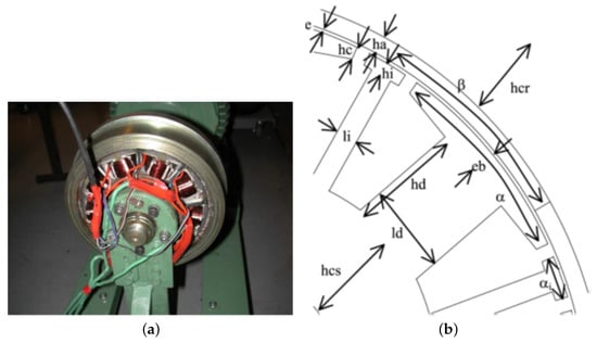
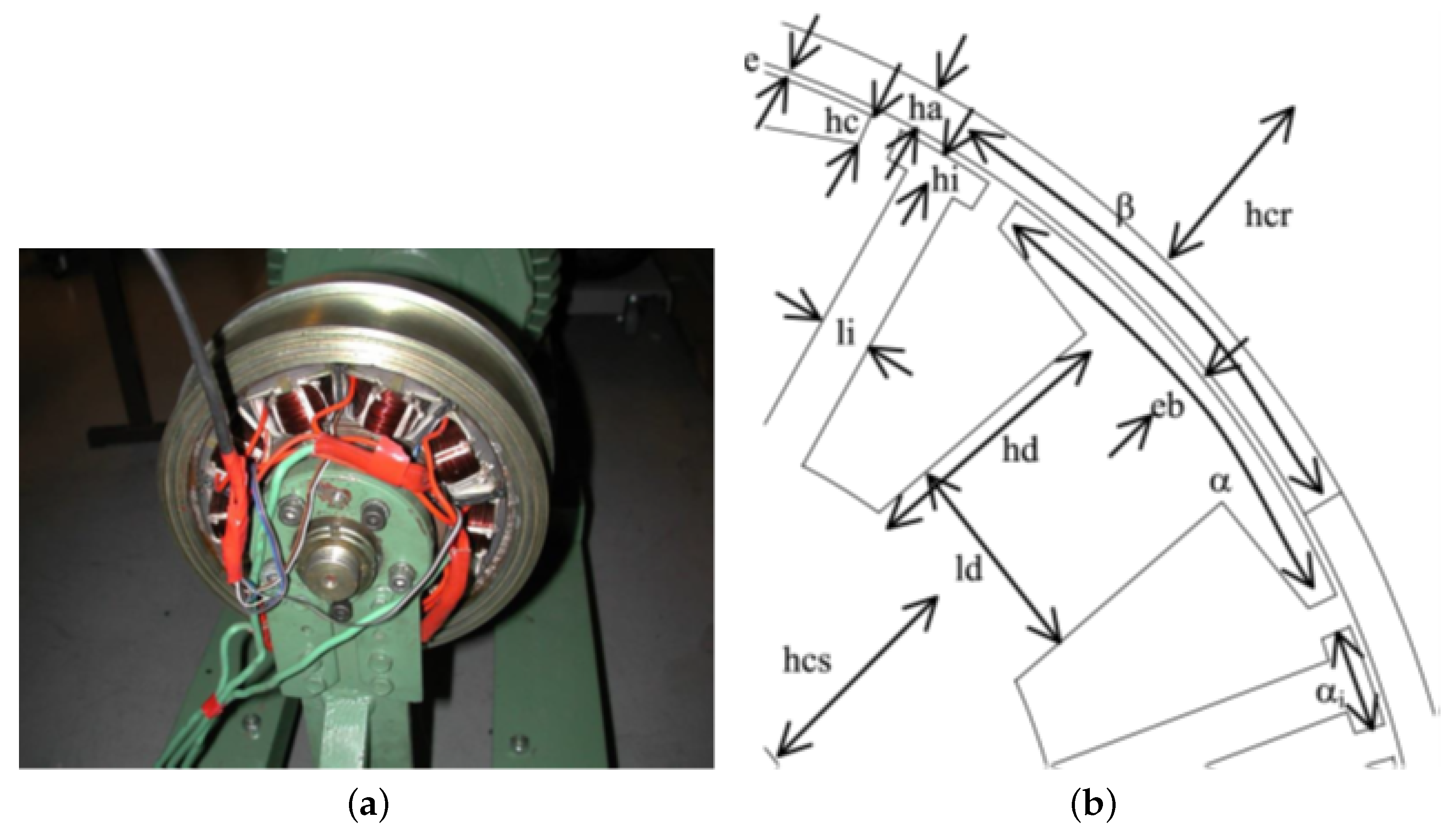
The first benchmark considered in this paper is the Brushless DC wheel motor (BLDC), which is based on an in-wheel motor for a solar racing vehicle, originally introduced in [38]. The benchmark involves five decision variables and a single objective, maximizing the efficiency [38]. The machine layout and the five variables are illustrated in Figure 2, while their admissible ranges are provided in Table 2.

Figure 2. Illustration of the BLDC motor benchmark showing (a) The prototype of the wheel motor, and (b) the geometric parameters of the BLDC motor [38].

Table 2. Numerical ranges for design variables of the BLDC benchmark.

Design Variable	Unit	Description	Min	Max
$B_d$	[T]	Teeth magnetic induction	0.9	1.8
$B_e$	[T]	Air-gap induction	0.50	0.76
$B_{cs}$	[T]	Stator back iron induction	0.6	1.6
$\delta$	[A/mm2]	Conductor current density	2.0	5.0
$D_s$	[mm]	Bore (stator) diameter	150	330

In addition to simple bound constraints on the variables, the formulation includes six inequality constraints reflecting the technological and operational limits of the motor in a wheel-hub application. The complete optimization problem can be formulated as follows:

$$\mathrm{OF}=-\eta ,$$

(8)

$$M_{\mathrm{tot}}\le 15 \mathrm{kg},$$

(9)

$$I_{max}\ge 125 \mathrm{A},$$

(10)

$$\mathrm{discr}(D_s,\delta ,B_d,B_e)\ge 0,$$

(11)

$$D_{\mathrm{ext}}\le 340 \mathrm{mm},$$

(12)

$$D_{\mathrm{int}}\ge 76 \mathrm{mm},$$

(13)

$$T_a\le 120 °\mathrm{C},$$

(14)

The objective function is expressed with a negative sign to convert the original maximization problem into a minimization framework. Here, $\eta$ denotes the efficiency, $M_{\mathrm{tot}}$ is the mass of the active components, and $D_{\mathrm{ext}}$ and $D_{\mathrm{int}}$ represent the external and internal diameters, respectively. The parameter $I_{max}$ corresponds to the phase current, while $T_a$ denotes the temperature of the magnets. The function $\mathrm{discr}(D_s,\delta ,B_d,B_e)$ is a discriminant used in the calculation of the slot height.

A key advantage of the BLDC benchmark is that the developers have provided source code for evaluating both the objective function and the constraints, ensuring that comparisons between optimization algorithms are not affected by implementation differences.

3.2. Loney’s Solenoid Benchmark

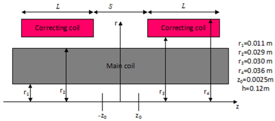
Loney’s solenoid is widely recognized as a standard benchmark in the optimal design of EMDs, primarily due to its simplified geometry and limited number of design parameters [39]. As illustrated in Figure 3, the solenoid consists of three coaxial coils: one central coil acting as the primary winding and two identical outer coils serving as correction windings.

Figure 3. Illustration of Loney’s solenoid benchmark.

The main coil is characterized by its inner and outer radii, denoted by $r_1$ and $r_2$, respectively, and its axial length h. Each correction coil has inner and outer radii $r_3$ and $r_4$, respectively, and a length L. These correction coils are symmetrically positioned on either side of the main coil along the z-axis, separated by a distance S.

The optimization problem consists of determining the optimal values of L and S such that a uniform magnetic flux density B is achieved over a specified segment of the solenoid’s central axis [39]. This requirement transforms the configuration of the correction coils into a well-defined design optimization problem. The objective function is defined as:

$$\mathrm{OF}={\displaystyle \frac{B_{max}-B_{min}}{B_0}}$$

(15)

where $B_{max}$ and $B_{min}$ denote the maximum and minimum magnetic flux densities, respectively, within the interval $(-z_0,z_0)$, and $B_0$ represents the magnetic flux density at the center of the solenoid ($z=0$).

3.3. TEAM22 Benchmark

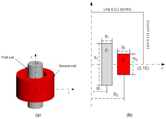
The TEAM Workshop Problem 22 (commonly referred to as TEAM22) addresses the optimal design of a Superconducting Magnetic Energy Storage (SMES) system, as illustrated in Figure 4. The optimization objective is twofold: to obtain a configuration that stores an amount of energy as close as possible to a prescribed reference value while simultaneously minimizing the stray magnetic field below another specified reference.

Figure 4. Illustration of the TEAM22 benchmark: (a) 3D representation of the SMES device; (b) right-half transverse cut of the SMES device.

This benchmark is available in two versions that differ in the number of design variables. In this study, the continuous and constrained version with eight design variables is considered, as shown in Figure 4, with their limits given in Table 3. The formulation includes two main constraints: (i) a geometrical constraint to ensure that the solenoids do not overlap, and (ii) a physical constraint to prevent the superconducting material from exceeding the quench limit defined by the admissible relationship between current density and peak magnetic flux density. Accordingly, the optimization problem can be formulated as follows [40,41]:

$$\mathrm{OF}={\displaystyle \frac{B_{\mathrm{stray}}^2}{B_{\mathrm{norm}}^2}}+w{\displaystyle \frac{\left|E-E_{\mathrm{ref}}\right|}{E_{\mathrm{ref}}}},$$

(16)

$$B_{\mathrm{stray}}^2={\displaystyle \frac{{\sum }_{i=1}^{22}{\left|B_{\mathrm{stray},i}\right|}^2}{22}},$$

(17)

$$R_1+{\displaystyle \frac{d_1}{2}}<R_2-{\displaystyle \frac{d_2}{2}},$$

(18)

$$\left|\mathbf{J}\right|=\left(-6.4\left|B_{max}\right|+54\right)\mathrm{A}/{\mathrm{mm}}^2,$$

(19)

Table 3. Design variables for the eight-parameter TEAM22 benchmark.

Design Variable	Unit	Min	Max
$R_1$	m	1.0	4.0
$R_2$	m	1.8	5.0
$h_{12}$	m	0.2	3.6
$h_{22}$	m	0.2	3.6
$d_1$	m	0.1	0.8
$d_2$	m	0.1	0.8
$J_1$	MA/m2	10	30
$J_2$	MA/m2	−30	−10

Here, $E_{\mathrm{ref}}$ denotes the target stored energy, fixed at $180 \mathrm{MJ}$, while $B_{\mathrm{norm}}$ is the reference stray magnetic field, set to $200 \mathsf{\mu }\mathrm{T}$. The quantity $B_{max}$ represents the peak magnetic flux density, and w is a weighting coefficient, set to 100 as proposed in [41], to balance the relative influence of the two terms of the objective function, namely the energy deviation and the stray field error. This choice prevents one term from dominating the optimization process.

The stray magnetic field, $B_{\mathrm{stray}}$, is evaluated using measurements taken at 22 equally spaced points along lines a and b, as shown in Figure 4.

3.4. Safety Transformer Benchmark

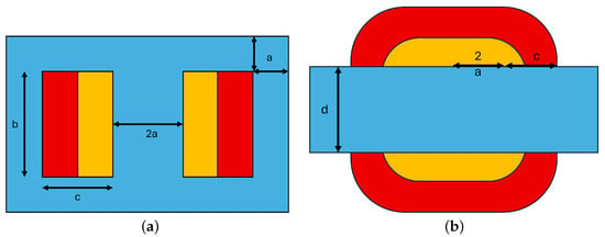
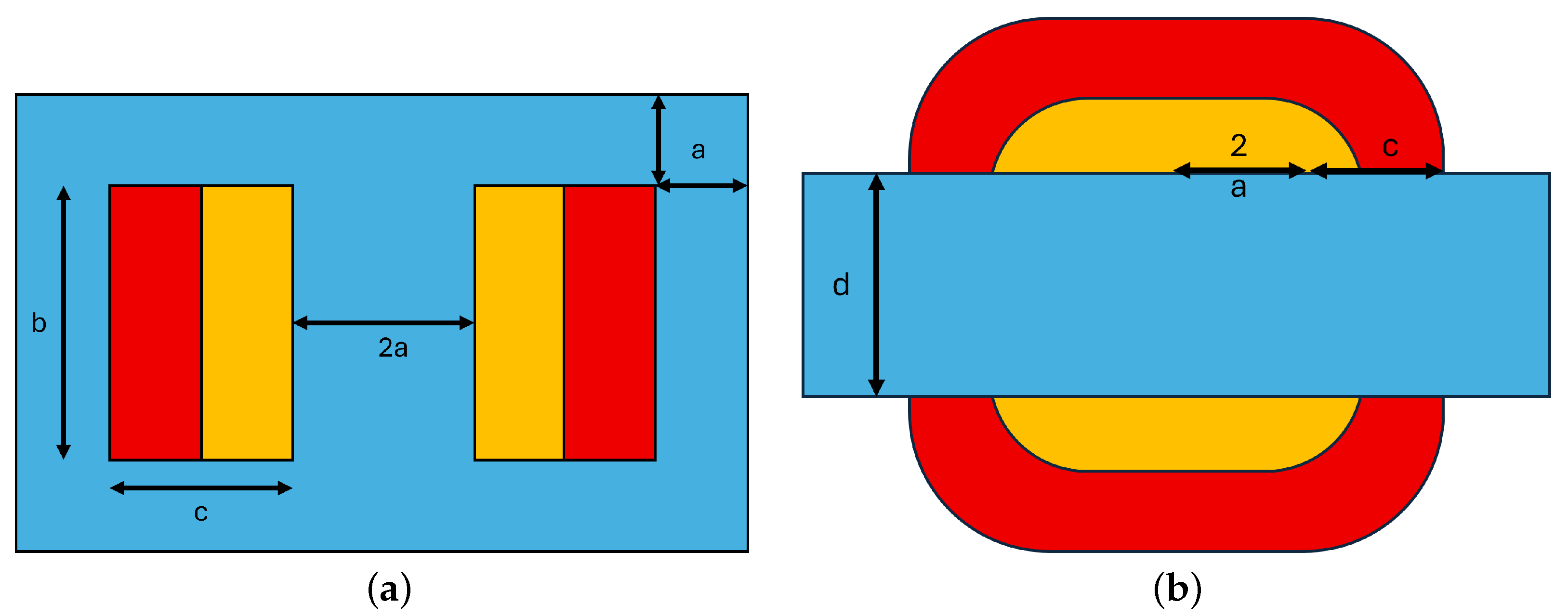
The safety transformer benchmark is formulated as a multidisciplinary optimization problem involving coupled thermal, electrical, and magnetic phenomena. These interactions are modeled through a set of nonlinear equations derived under the following assumptions: uniform magnetic induction in the iron core, negligible voltage drop due to the magnetizing current, and a vertical magnetic field distribution within the coils. Under these assumptions, the model results in an implicit system of eight coupled multi-physical equations, along with additional equations solved sequentially. This benchmark is highly constrained and representative of real-world electromagnetic design problems.

To efficiently manage the coupling between different physical domains, the Individual Discipline Feasible (IDF) formulation is adopted. In this approach, the coupling is relaxed and enforced through auxiliary variables and equality constraints, allowing each discipline to be solved only once per function evaluation, thereby significantly reducing computational cost.

The objective is to minimize the total mass of active materials. The optimization problem is formulated as follows [42,43]:

$$\mathrm{OF}=M_{\mathrm{tot}},$$

(20)

$$T_{\mathrm{cond}}\le 120 °\mathrm{C},$$

(21)

$$T_{\mathrm{iron}}\le 100 °\mathrm{C},$$

(22)

$${\displaystyle \frac{I_{10}}{I_1}}\le 0.1,$$

(23)

$${\displaystyle \frac{\mathsf{\Delta }{V}_2}{V_{20}}}\le 0.1,$$

(24)

$$f_1\le 1,$$

(25)

$$f_2\le 1,$$

(26)

$$\eta \ge 0.8,$$

(27)

$$40 °\mathrm{C}\le T_{\mathrm{cond},\mathrm{IDF}}\le 400 °\mathrm{C},$$

(28)

$$0.1 \mathrm{V}\le \mathsf{\Delta }{V}_{2,\mathrm{IDF}}\le 24 \mathrm{V}$$

(29)

where $M_{\mathrm{tot}}$ is the total mass of the transformer; $T_{\mathrm{cond}}$ and $T_{\mathrm{iron}}$ denote the conductor and core temperatures, respectively; ${\displaystyle \frac{I_{10}}{I_1}}$ is the current ratio; ${\displaystyle \frac{\mathsf{\Delta }{V}_2}{V_{20}}}$ represents the relative voltage drop; $f_1$ and $f_2$ are the primary and secondary winding fill factors; and $\eta$ is the efficiency. The variables $T_{\mathrm{cond},\mathrm{IDF}}$ and $\mathsf{\Delta }{V}_{2,\mathrm{IDF}}$ are auxiliary variables introduced in the IDF formulation. This benchmark is illustrated in Figure 5, and the design variables are tabulated in Table 4.

Figure 5. Illustration of the safety transformer benchmark, (a) Cross-sectional representation transformer; (b) Top-view representation.

Table 4. Design variables and their limits for the safety transformer benchmark.

Design Variable	Unit	Min	Max
a	mm	3	30
b	mm	14	95
c	mm	6	40
d	mm	10	80
$n_1$	–	200	1200
$S_1$	mm2	0.15	19
$S_2$	mm2	0.15	19

3.5. C-Core Benchmark

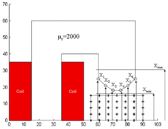
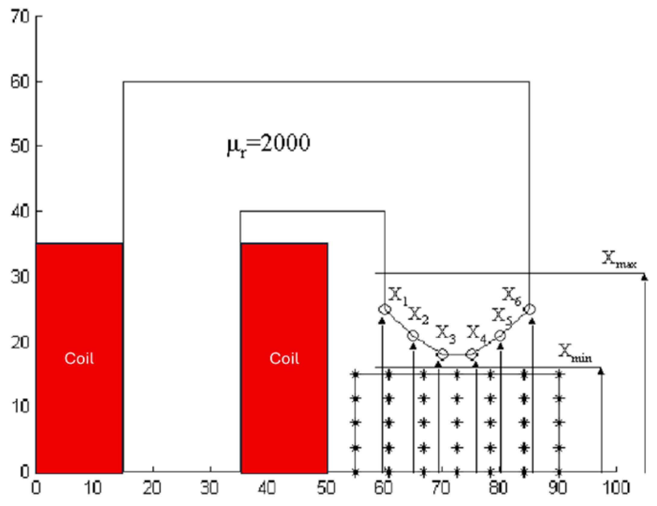
The C-Core benchmark focuses on shaping the pole faces of a magnetic core to achieve a uniform magnetic field distribution within a rectangular region located at the center of the air gap [44,45]. The geometry, constraints, and evaluation grid are illustrated in Figure 6.

Figure 6. Illustration of the C-Core benchmark.

The design variables correspond to the horizontal coordinates of six control points $x_1,x_2,\dots ,x_6$, which define the pole face profile. The magnetic flux density is evaluated at 35 grid points using FEM.

The objective function is defined as:

$$\mathrm{OF}=-{\displaystyle \sum _{i=1}^{35}}{\displaystyle \frac{|B_0-B_i|}{B_0}},$$

(30)

where $B_i$ is the magnetic flux density at the i-th point, and $B_0$ is the value at the center.

The design variables satisfy:

$$18\le x_j\le 30 j=1,\dots ,6$$

(31)

3.6. Magnetizer Benchmark Problem

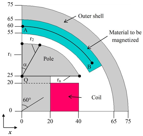
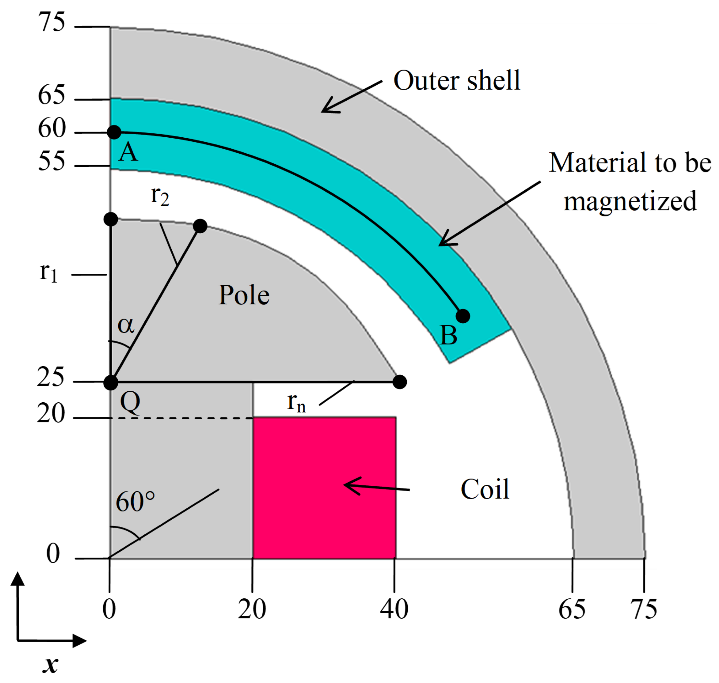
The magnetizer benchmark is formulated as a two-dimensional linear magnetostatic field analysis using the FEM. The geometry under consideration is depicted in Figure 7 [44]. Within the FEM model, the object intended for magnetization, which is composed of a nonmagnetic material, is assigned a relative permeability close to that of air. In contrast, a much higher permeability value, ${\mu }_r=1000$, is assigned to the pole face and outer shell regions. A large current density of $5 \mathrm{A}/{\mathrm{mm}}^2$ is applied to the coil region to drive the magnetostatic behavior.

Figure 7. Illustration of the magnetizer benchmark.

To define the shape of the pole face, this study employs uniform non-rational cubic B-splines (UNBS) governed by several control points, denoted by $P_1$ through $P_4$. These control points are angularly spaced by $\alpha =30°$ and are allowed to move radially outward from a fixed reference point Q. Consequently, this configuration involves four design variables, $r_1$, $r_2$, $r_3$, and $r_4$, corresponding to the radial distances of each control point from Q, with their allowable ranges given in Table 5. Once the positions of these control points are specified, the pole face geometry is generated from the resulting B-spline curve. It is worth noting that the spline is constructed such that it passes through control points $P_1$ and $P_4$, each of which is represented by three coincident control points to ensure geometric continuity at the two ends.

Table 5. Ranges of design variables used in the magnetizer problem.

Design Variable	Unit	Min	Max
$r_1$	mm	22.0	29.5
$r_2$	mm	22.0	31.25
$r_3$	mm	22.0	38.7
$r_4$	mm	22.0	48.5

The objective of this optimization problem is to obtain a uniform magnetic flux density distribution along the chord $AB$. To promote the existence of multiple optimal solutions, the exact target value of the uniform magnetic flux density is intentionally left unspecified [23]. Accordingly, the objective function is defined as

$$\mathrm{OF}={\displaystyle \frac{{\sigma }_B}{\overline{B}}}$$

(32)

where ${\sigma }_B$ and $\overline{B}$ denote the standard deviation and mean of the magnetic flux density distribution along chord $AB$, respectively. The magnetic flux density is evaluated at N points along this chord. Thus, the objective function can be rewritten in the following compact form:

$$\mathrm{OF}={\displaystyle \frac{\sqrt{\frac{1}{N}{\sum }_{i=1}^N{\left(B_i-\overline{B}\right)}^2}}{\overline{B}}}$$

(33)

where

$$\overline{B}={\displaystyle \frac{1}{N}}{\displaystyle \sum _{i=1}^N}{B}_i$$

(34)

and

$$B_i=B\left({\theta }_i\right),\hspace{1em}\hspace{1em}35°\le {\theta }_i\le 89°$$

(35)

$${\theta }_i={\theta }_1+(i-1)h,\hspace{1em}\hspace{1em}i=1,2,\dots ,N$$

(36)

$$h={\displaystyle \frac{{\theta }_N-{\theta }_1}{N-1}}$$

(37)

where $B_i$ represents the magnetic flux density at the ith sampling point along chord $AB$, and a total of $N=50$ equally spaced points are considered.

4. Comparison and Performance Evaluation Procedure

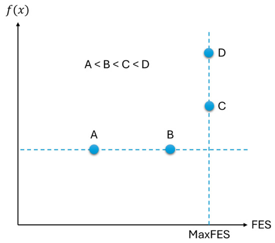
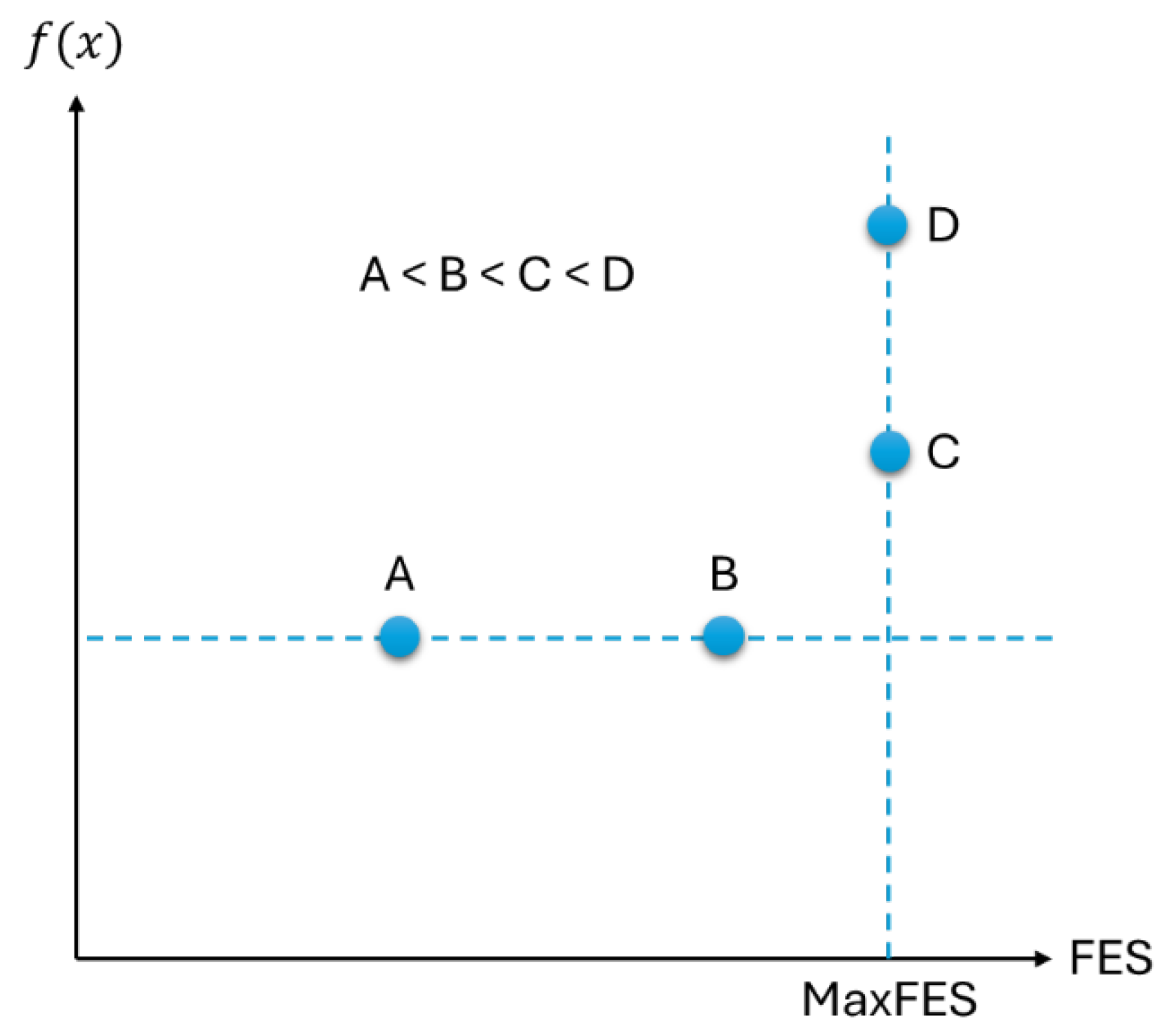
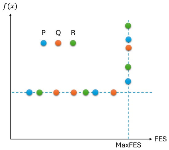
The performance assessment in this study follows the evaluation criteria established for the CEC 2022 Special Session and Competition on Single-Objective Bound-Constrained Numerical Optimization. This criterion accounts for both solution accuracy and computational efficiency. It employs the Wilcoxon rank-sum test [46] (also known as the Mann–Whitney U test [46]) to statistically compare results. As illustrated in Figure 8, the method ranks trials from best to worst, where smaller objective values indicate better performance.

Figure 8. Trials sampled on the terminal axes can be ranked from best to worst. Since smaller values indicate better performance, Trial A ranks highest.

For a given benchmark function f, let ${\mathbf{T}}_{i,a,f}$ represent the result of the i-th trial ($i=1,2,\dots ,N$) of algorithm a ($a=1,2,\dots ,M$), where N is the number of trials (e.g., 25) and M is the number of algorithms. All $N\times M$ trials are ranked from best to worst, with the best assigned rank $N\times M$ and the worst assigned rank 1. Ties are assigned the average rank.

The score of algorithm a for function f is computed as:

$$S_{a,f}={\displaystyle \sum _{i=1}^N}{\mathrm{rank}}_{i,a,f}-{\displaystyle \frac{N(N+1)}{2}}$$

(38)

This process is repeated for all benchmark functions, and the final score is obtained by summing over all functions. Higher scores indicate better performance.

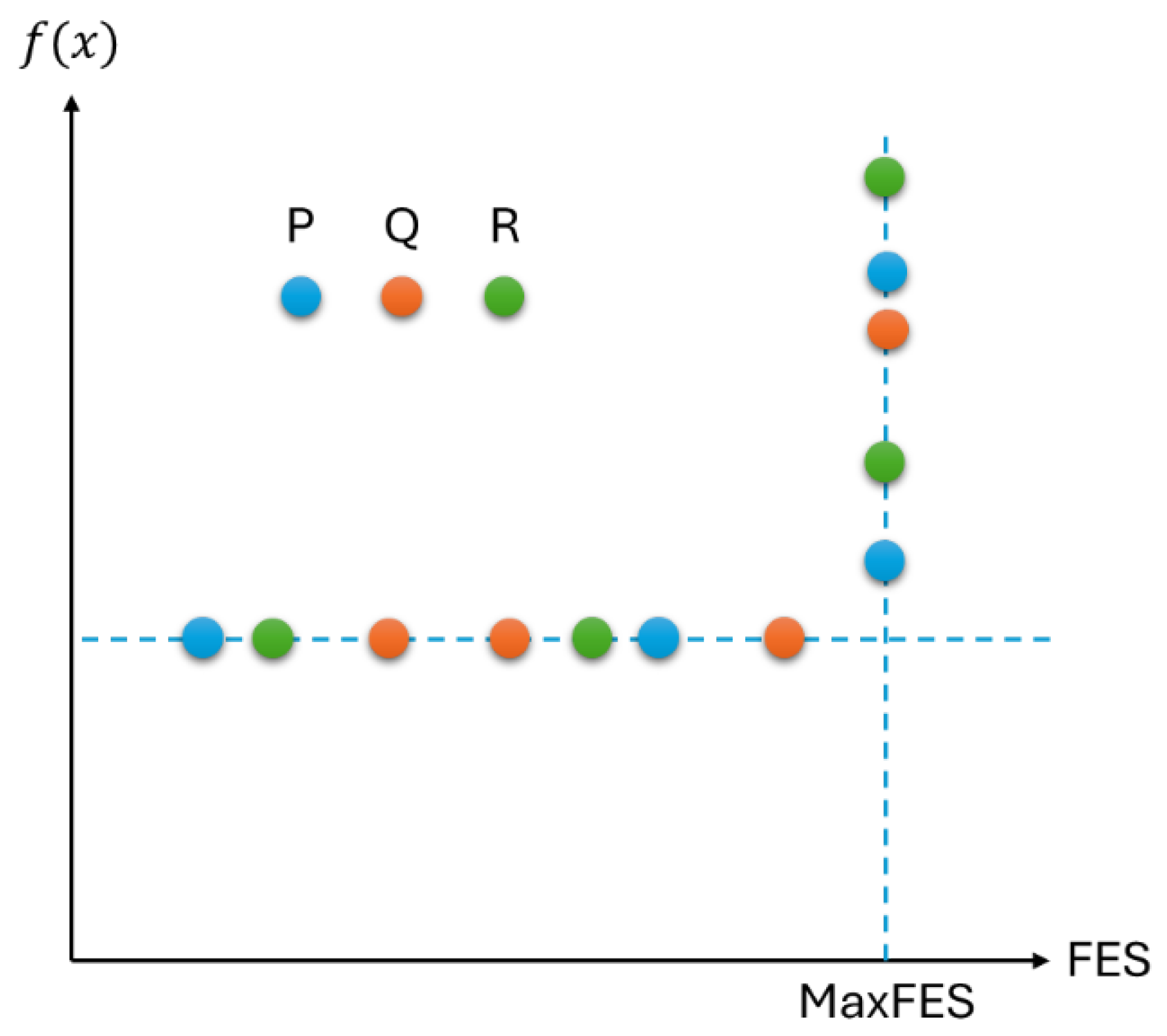
Figure 9 illustrates an example with three algorithms (P, Q, and R), each performing four trials ($N=4$) on the same benchmark function. All $4\times 3=12$ trial results are ranked from best to worst, with rank 12 assigned to the best trial and rank 1 to the worst. Ties, if present, would be assigned the average of their rank positions. Table 6 shows the ranks for each trial and the corresponding Sum of Ranks (SR) for each algorithm. For example, Algorithm P’s four trials received ranks 12, 7, 5, and 2, giving a sum of ranks of $12+7+5+2=26$. Similarly, Algorithm Q’s four trials sum to 28, and Algorithm R’s to 24.

Figure 9. Example illustrating the ranking-based scoring method for a single benchmark function.

Table 6. Rank assignments and function score calculation.

Trial	P	Q	R
12	12
11			11
10		10
9		9
8			8
7	7
6		6
5	5
4			4
3		3
2	2
1			1
SR	26	28	24
SR-10	16	18	14

To calculate the function score for each algorithm, we subtract the correction term:

$${\displaystyle \frac{N(N+1)}{2}}={\displaystyle \frac{4\times 5}{2}}=10.$$

(39)

This correction term corresponds to the minimum sum of ranks an algorithm would receive if all its trials were the worst possible. Higher scores indicate stronger performance. In this example, Algorithm Q achieves the highest score (18), meaning it consistently outperformed the other algorithms across its trials. In statistical terms, the score represents the number of pairwise “wins” an algorithm has over all other algorithms’ trials for the same function. In the case of only two algorithms, this scoring method reduces to the well-known Mann–Whitney U-statistic.

5. Results and Discussion

The proposed algorithm (MuCAO), along with the modern metaheuristics presented in Section 2.1 and the reference metaheuristics described in Section 2.3, have been evaluated using two applications. All algorithms were executed in parallel on an Intel Core i7-based system, and the implementations were done using the commercial software MATLAB 2025b. The parameter settings of each algorithm used in this study are given in Table 7. It is worth mentioning that the initialization strategy is unified for all algorithms, such that the initial population for all algorithms was generated randomly within the feasible search space defined by the lower and upper bounds of the problem variables. The stopping criterion was based on the maximum number of function evaluations. Furthermore, for constraint handling, each algorithm was implemented using its original constraint-handling mechanism whenever such a technique was explicitly defined in the corresponding method. For algorithms that do not include a specific constraint-handling strategy, a penalty-based method was adopted to handle constraint violations. Finally, for the parallel implementation, stochastic numbers were generated using MATLAB’s mrg32k3a pseudo-random number generator. A distinct deterministic substream was assigned to each independent run thereby ensuring non-overlapping and reproducible random sequences across parallel runs.

Table 7. Parameter setting values for the different algorithms.

Algorithm	Parameter Name	Value/Expression
All algorithms	Population size	50
	Number of iterations	1000
	Maximum number of evaluations	20,000
AFT	${\alpha }_0,{\alpha }_1$	$1.0, 2.0$
	${\beta }_0,{\beta }_1$	$0.1, 2.0$
AHA	Migration coefficient	$2n$
BBO	Habitat modification probability	1
	Immigration probability bounds for each gene	$[0, 1]$
	Mutation probability	0
	Maximum migration rate	1
	Maximum immigration rate	1
	Step size for numerical integration of probabilities	1
DE	F	0.5
	$CR$	0.9
GEO	$p_a$: Propensity to attack	$[0.5, 2]$
	$p_c$: Propensity to cruise	$[1, 0.5]$
GWO	a: Control parameter	$[2, 0]$
HGS	E: Variation control parameter	0.03
POA	I: Control parameter	Randomly selected from $\{1,2\}$
	R: Constant	0.2
PSO	$c_1,c_2$	$1.8, 2$
	w	$[0.9, 0.1]$
RSO	Internal parameters	None
SSA	$c_1$: Control parameter	0.5
TDO	Internal parameters	None
TLBO	Internal parameters	None
TTA	$pro{b}_{lost}$: Probability of ball loss	$[0.1, 0.3]$
	$c_1,c_3$: Coefficients	$[0.5, 1.5]$
	$c_2$: Coefficient	$[1.0, 2.5]$
	TeamsSize: Number of teams in the league	5
WSO	$f_{min},f_{max}$	$0.07, 0.75$
	$\tau$	4.125
	$a_0,a_1,a_2$	$6.25, 100, 0.0005$
ZOA	Internal parameters	None

5.1. Application #1: Selected Benchmarks

The results are summarized in Table 8 and Table 9. As previously mentioned, the comparative methodology adopted in this study aligns with the standard protocol used in the CEC 2022 competition for benchmarking optimization algorithms. The following key observations can be drawn:

Table 8. Scores and ranks of tested algorithms.

Algorithm	S1 *	R1 *	S2	R2	S3	R3	S4	R4	S5	R5	S6	R6	Score	Rank
MuCAO	8666	2	8883	3	8696.5	2	9501	2	7891	4	6897	6	50,534.5	1
WSO	6703	5	9954	1	9273.5	1	9558	1	6512	9	6408	8	48,408.5	2
TDO	9464	1	8046	4	7403.5	5	5584	9	9822	1	7756	3	48,075.5	3
AHA	6423	8	7690	5	8600.5	3	9312	3	4788	10	6540	7	43,353.5	4
DE	6101	9	9818	2	8004.5	4	5368	10	8024.5	3	3850	14	41,166	5
POA	7745	3	5962	7	6932.5	7	6620	6	7545	6	6149	9	40,953.5	6
TTA	3330	14	5835	9	6936.5	6	7112	4	6896	8	8631	1	38,740.5	7
MVPA	6557	7	6921	6	4530.5	11	4917	12	9323	2	3489	15	35,737.5	8
HGS	5501	10	5402	10	4238.5	13	2727	16	7642	5	7827	2	33,337.5	9
AFT	4433	11	5860	8	6840	8	6099	7	3592	12	3852	13	30,676	10
ZOA	7663	4	4091	12	4746.5	10	3048	14	3888	11	5187	10	28,623.5	11
GWO	3677	13	2823	14	4527.5	12	6710	5	3298	13	7111	5	28,146.5	12
PSO	6570	6	4380	11	2685.5	14	2802	15	7125.5	7	3083	16	26,646	13
BBO	2558	16	3503	13	5312.5	9	4975	11	1984	15	4515	12	22,847.5	14
GEO	4127	12	1196	16	1701.5	16	3626	13	3119	14	7380	4	21,149.5	15
SSA	3084	15	2030	15	2588.5	15	5719	8	1280	16	4797	11	19,498.5	16
RSO	563	17	659	17	913.5	17	390	17	612	17	608	17	3745.5	17
TLBO	122	18	20	18	338.5	18	322	18	13	18	33	18	848.5	18

* $S_i$ = Score on function i, $R_i$ = Rank on function i.

Table 9. Time comparison of tested algorithms.

Algorithm	Loney [s]	BLDC [s]	Safety Transformer [s]	TEAM22 [hh:mm:ss]	CCore [hh:mm:ss]	Magnetizer [hh:mm:ss]
MuCAO	1.83	3.75	7.18	00:42:06	03:12:34	01:12:27
WSO	2.00	3.72	6.55	00:40:56	04:16:35	01:19:21
TDO	1.68	3.33	6.22	00:41:18	04:26:37	01:13:52
AHA	2.22	3.95	6.86	00:37:37	04:27:35	01:11:23
DE	2.01	3.63	6.55	00:56:23	04:21:58	01:22:16
POA	1.47	3.07	5.96	00:41:18	04:03:37	01:09:24
TTA	2.13	3.79	6.73	00:39:45	03:44:39	01:08:38
MVPA	4.40	5.83	9.16	00:44:59	04:34:18	01:35:18
HGS	1.77	3.39	6.36	00:41:07	03:44:56	01:15:43
AFT	2.07	4.21	6.66	00:36:59	03:43:21	01:13:46
ZOA	1.51	3.07	5.91	00:41:35	04:27:04	01:12:48
GWO	1.66	3.31	6.25	00:52:40	04:17:00	01:03:57
PSO	20.18	22.21	24.91	00:57:44	03:40:46	01:24:38
BBO	4.33	6.43	9.67	00:44:01	04:22:31	01:12:36
GEO	2.44	4.05	6.87	00:30:37	03:44:14	01:16:16
SSA	1.82	3.37	6.31	00:33:10	03:41:30	01:03:32
RSO	1.61	3.17	6.04	00:42:09	03:44:18	01:26:44
TLBO	4.16	6.91	11.88	01:02:11	05:26:16	02:07:53

• MuCAO, the proposed algorithm, achieved the highest cumulative performance score of 50,534.5, making it the best performer overall. It consistently ranked 2nd on Benchmarks 1, 3, and 4; 3rd on Benchmark 2; 4th on Benchmark 5; and 6th on Benchmark 6. This consistent ranking demonstrates MuCAO’s strong generalization ability and robustness across diverse problem types.
• WSO secured the second position overall, with a cumulative score of 48,408.5. It ranked 1st on Benchmarks 2, 3, and 4, demonstrating its effectiveness on those specific problems. However, it showed weaker performance on Benchmarks 5 and 6, ranking 9th and 8th respectively, which negatively impacted its final score.
• TDO ranked third, with a total score of 48,075.5, very close to that of WSO. It achieved 1st place on Benchmarks 1 and 5 but dropped significantly to 9th place on Benchmark 4, which affected its overall standing. Nevertheless, TDO remained competitive across most benchmarks.
• Among the reference algorithms, DE emerged as the best, ranking 5th overall with a cumulative score of 41,166. The next best reference algorithm was MVPA, which ranked 7th with a score of 35,737.5. On the other hand, PSO, BBO, SSA, and TLBO performed notably worse, ranking 13th, 14th, 16th, and 18th (last), respectively.
• WSO was the most frequent top performer, achieving 1st place in three benchmarks. It was followed by TDO, which ranked 1st in two benchmarks, and TTA, which achieved 1st place in one benchmark.
• Notably, MuCAO had the smallest variation in ranking across all benchmarks, with its best rank being 2nd and its worst 6th. This limited variation highlights the algorithm’s consistency and adaptability.
• The RSO algorithm ranked 17th overall, placing it second to last, while TLBO consistently ranked last (18th) in all benchmarks, marking it as the poorest performer.
• No algorithm ranked first across all benchmarks, emphasizing that no single algorithm demonstrates universal superiority. This reinforces the commonly accepted view that algorithm performance is problem-dependent and that a “one-size-fits-all” solution does not exist in optimization.
• Some algorithms, despite being recently developed and claimed by their authors to be superior to many classical algorithms, exhibit relatively poor performance for the optimal design of EMDs. For example, GEO was ranked 15th out of 18, and RSO ranked 17th, indicating their limited effectiveness for the tested benchmarks.

Table 9 presents the overall simulation times accumulated over 25 runs for each algorithm and benchmark. It is important to note that the reported times reflect the total runtime for each simulation set, not individual runs. Key observations include:

• The MuCAO algorithm showed good computational efficiency, combining high performance with acceptable runtime.
• The least efficient algorithms in terms of computing time were MVPA, PSO, BBO, and TLBO, all of which belong to the set of reference algorithms. Their relatively poor performance is compounded by high computational costs.
• A significant difference was observed between benchmarks based on analytical models and those involving FEM simulations. This suggests the practical importance of using analytical or surrogate models to reduce computation time in the design and optimization of EMDs.
• The most time-consuming benchmark was the C-Core optimization problem, which took an average of 4 h, 6 min, and 39 s to simulate and optimize. This was followed by the Magnetizer problem, with an average runtime of 1 h, 18 min, and 22 s.
• The longest single runtime was recorded by TLBO on the C-Core benchmark, with a total time of 5 h, 26 min, and 16 s. In contrast, the shortest runtime was achieved by POA on the Loney benchmark, completing in just 1.45 s.

To complement the cumulative ranking analysis and provide a clearer head-to-head statistical perspective, an additional pairwise comparison was carried out between the proposed MuCAO and the four strongest competing algorithms, namely WSO, TDO, AHA, and DE, and the results are reported in Table 10. This analysis was included because overall ranking scores, although informative, may not fully reveal the direct comparative differences between the best-performing methods. The results of the pairwise comparison show that MuCAO achieved the first rank in all four cases, with total scores of 1944, 2150, 2640, and 2250 against 1806, 1600, 1110, and 1500 for WSO, TDO, AHA, and DE, respectively. These results indicate that the superiority of MuCAO is not only reflected in the cumulative multi-algorithm ranking framework but is also preserved in direct comparisons with the strongest competing algorithms.

Table 10. Pairwise comparison between MuCAO and the best comparing algorithms.

Case	Algorithm	Score1	Score2	Score3	Score4	Score5	Score6	Total Score	Rank
MuCAO vs. WSO	MuCAO	146	516	281	233	412	356	1944	1
	WSO	479	109	344	392	213	269	1806	2
	p-value	0.001278	$8.19\times {10}^{-5}$	0.5475	0.1253	0.05475	0.4041	–	–
MuCAO vs. TDO	MuCAO	441	234	608	494	137	236	2150	1
	TDO	184	391	17	131	488	389	1600	2
	p-value	0.01301	0.1302	$1.041\times {10}^{-8}$	0.0004449	0.000685	0.1403	–	–
MuCAO vs. AHA	MuCAO	489	523	383	349	549	347	2640	1
	AHA	136	102	242	276	76	278	1110	2
	p-value	0.0006381	$4.609\times {10}^{-5}$	0.1744	0.4849	$4.67\times {10}^{-6}$	0.5094	–	–
MuCAO vs. DE	MuCAO	100	515	550	299	308	478	2250	1
	DE	525	110	75	326	317	147	1500	2
	p-value	$3.899\times {10}^{-5}$	$8.874\times {10}^{-5}$	$4.256\times {10}^{-6}$	0.8009	0.9381	0.001367	–	–

In addition, the corresponding p-values obtained from the Wilcoxon rank-sum test are also reported in Table 10 in order to assess the statistical significance of the observed differences. For the comparison between MuCAO and WSO, statistically significant differences are observed on Benchmarks 1 and 2 only, whereas the remaining benchmarks do not show significant differences at the 5% significance level. For the comparison with TDO, statistically significant differences are obtained on Benchmarks 1, 3, 4, and 5, while for AHA the significant differences appear on Benchmarks 1, 2, and 5. Similarly, in the comparison with DE, statistically significant differences are observed on Benchmarks 1, 2, 3, and 6. Overall, these results show that although the statistical significance of the differences is benchmark-dependent, MuCAO maintains a stronger aggregate performance than the strongest competing algorithms and demonstrates a consistent advantage in the direct pairwise comparisons.

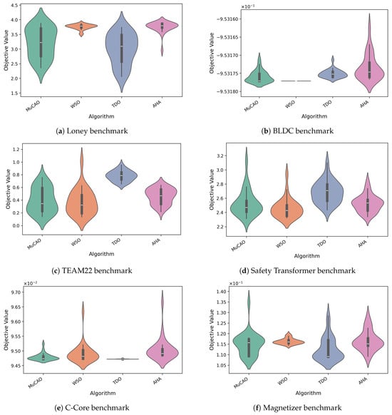
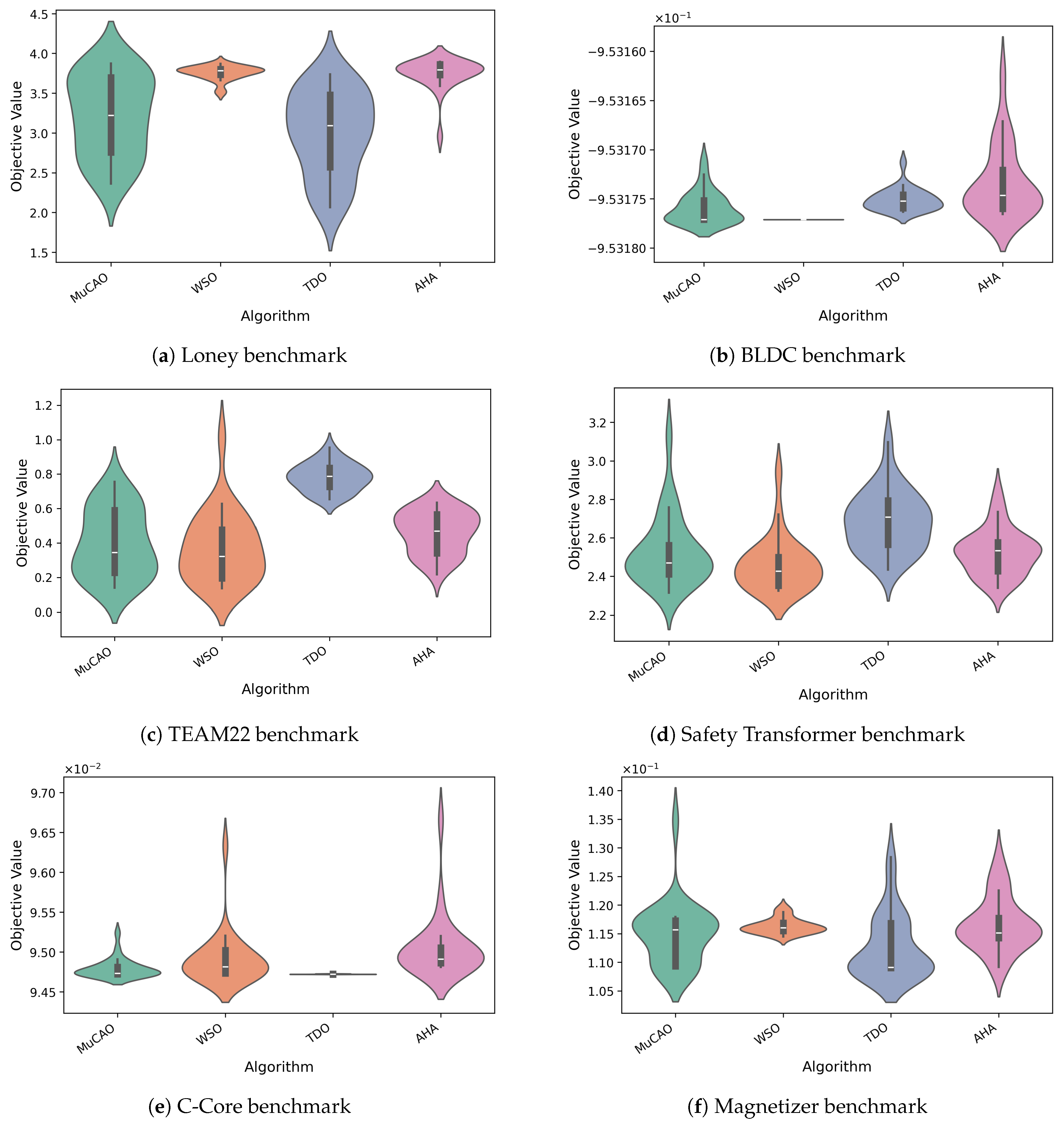
To further illustrate the performance variability and stability of the top-performing algorithms, violin plots of the results for the best four algorithms across all benchmarks and 25 independent runs are presented in Figure 10. These plots provide insight into the distribution, spread, and consistency of the obtained objective function values, offering a complementary perspective to the average performance scores.

Figure 10. Violin plots of the best four algorithms for all six benchmarks.

It is also worth noting that in some cases, the violin plots appear extremely narrow, almost as vertical lines, indicating exceptionally low variability in the algorithm’s performance across the 25 independent runs. Two notable examples are WSO on the BLDC benchmark and TDO on the C-Core benchmark. In both cases, the respective algorithms consistently produced nearly identical objective function values, reflecting a highly stable optimization behavior. Interestingly, these algorithms were also ranked first on their corresponding benchmarks, suggesting that their convergence was not only stable but also highly effective in achieving optimal or near-optimal solutions. This reinforces the reliability of these algorithms for those specific problem types and highlights their potential suitability for similar optimization tasks in real-world EMDs.

Additional performance statistics, including the best, mean, median, standard deviation, and worst values obtained by all algorithms, are reported in Table 11, Table 12, Table 13, Table 14, Table 15 and Table 16.

Table 11. Additional statistical results of tested algorithms for the Loney Benchmark.

Algorithm	Final Rank	Total Score	Best	Mean	Median	Standard Deviation	Worst
MuCAO	1	50,534.5	2.3608	3.2103	3.2220	0.5044	3.8735
WSO	2	48,408.5	3.5126	3.7561	3.7849	0.0898	3.8701
TDO	3	48,075.5	2.0659	2.9958	3.0922	0.5191	3.7361
AHA	4	43,353.5	2.9566	3.7485	3.7953	0.1909	3.8949
DE	5	41,166	2.6607	3.7144	3.8261	0.3124	3.9526
POA	6	40,953.5	2.2616	3.3947	3.6641	0.5162	3.9254
TTA	7	38,740.5	3.7446	3.9731	3.9797	0.0789	4.1213
MVPA	8	35,737.5	2.4280	3.6443	3.7578	0.3831	3.9526
HGS	9	33,337.5	2.3413	13.8584	3.9244	41.1231	208.0063
AFT	10	30,676	2.4542	3.6255	3.7468	0.3704	3.9444
ZOA	11	28,623.5	2.3381	3.4263	3.5467	0.5006	3.9342
GWO	12	28,146.5	2.3921	4.3716	4.1034	1.0168	6.6917
PSO	13	26,646	2.2109	3.5629	3.7962	0.5070	3.9526
BBO	14	22,847.5	3.7014	4.2180	4.1111	0.4100	5.4164
GEO	15	21,149.5	2.8921	3.9383	3.9573	0.3356	4.6253
SSA	16	19,498.5	2.0972	4.2257	4.1698	0.7871	6.8597
RSO	17	3745.5	5.1904	172.0670	79.3468	243.4167	858.4330
TLBO	18	848.5	6.1809	5008.6977	995.0154	8674.0067	30,134.4622

Table 12. Additional statistical results of tested algorithms for the BLDC Benchmark.

Algorithm	Final Rank	Total Score	Best	Mean	Median	Standard Deviation	Worst
MuCAO	1	50,534.5	−0.9532	−0.9532	−0.9532	0.0000	−0.9532
WSO	2	48,408.5	−0.9532	−0.9532	−0.9532	0.0000	−0.9532
TDO	3	48,075.5	−0.9532	−0.9532	−0.9532	0.0000	−0.9532
AHA	4	43,353.5	−0.9532	−0.9532	−0.9532	0.0000	−0.9532
DE	5	41,166	−0.9532	−0.9532	−0.9532	0.0000	−0.9531
POA	6	40,953.5	−0.9532	−0.9531	−0.9532	0.0001	−0.9530
TTA	7	38,740.5	−0.9532	−0.9532	−0.9532	0.0000	−0.9531
MVPA	8	35,737.5	−0.9532	−0.9531	−0.9532	0.0002	−0.9522
HGS	9	33,337.5	−0.9532	−0.9531	−0.9531	0.0000	−0.9531
AFT	10	30,676	−0.9532	−0.9532	−0.9532	0.0000	−0.9532
ZOA	11	28,623.5	−0.9532	−0.9531	−0.9531	0.0001	−0.9529
GWO	12	28,146.5	−0.9530	−0.9528	−0.9528	0.0001	−0.9525
PSO	13	26,646	−0.9532	−0.9527	−0.9531	0.0006	−0.9514
BBO	14	22,847.5	−0.9531	−0.9529	−0.9530	0.0002	−0.9525
GEO	15	21,149.5	−0.9507	−0.9483	−0.9480	0.0013	−0.9455
SSA	16	19,498.5	−0.9528	−0.9519	−0.9519	0.0006	−0.9508
RSO	17	3745.5	−0.9507	−0.9156	−0.9406	0.0803	−0.6007
TLBO	18	848.5	−0.9439	240.5782	89.6648	285.9805	984.2205

Table 13. Additional statistical results of tested algorithms for the Safety Transformer Benchmark.

Algorithm	Final Rank	Total Score	Best	Mean	Median	Standard Deviation	Worst
MuCAO	1	50,534.5	2.3149	2.5294	2.4696	0.1804	3.1306
WSO	2	48,408.5	2.3253	2.4601	2.4274	0.1398	2.9425
TDO	3	48,075.5	2.4349	2.6848	2.7089	0.1547	3.0966
AHA	4	43,353.5	2.3407	2.5257	2.5337	0.1196	2.8340
DE	5	41,166	2.3397	3.1097	2.3988	2.3667	14.3405
POA	6	40,953.5	2.5185	2.7648	2.6876	0.1916	3.1895
TTA	7	38,740.5	2.4161	2.7558	2.7347	0.1631	3.0903
MVPA	8	35,737.5	2.7389	3.5460	3.2783	0.9234	7.4913
HGS	9	33,337.5	2.5355	3.6433	3.5547	0.6664	5.4559
AFT	10	30,676	2.3285	2.8692	2.4911	1.5511	10.2477
ZOA	11	28,623.5	2.6780	3.3484	3.2738	0.4239	4.1078
GWO	12	28,146.5	3.0527	3.3267	3.3254	0.1877	3.7577
PSO	13	26,646	3.0910	6.4675	5.1101	3.0843	14.6743
BBO	14	22,847.5	–	–	–	–	–
GEO	15	21,149.5	6.6817	10.0810	10.6338	1.5337	13.0240
SSA	16	19,498.5	3.7998	5.7278	5.4568	1.1294	8.0258
RSO	17	3745.5	14.4267	37.7453	32.1729	17.1507	84.5889
TLBO	18	848.5	39.2682	885.2601	334.9822	1418.7346	5166.6927

Table 14. Additional statistical results of tested algorithms for the TEAM22 Benchmark.

Algorithm	Final Rank	Total Score	Best	Mean	Median	Standard Deviation	Worst
MuCAO	1	50,534.5	0.1397	0.3962	0.3444	0.1934	0.7553
WSO	2	48,408.5	0.1367	0.3711	0.3230	0.2034	1.0145
TDO	3	48,075.5	0.6533	0.7811	0.7885	0.0803	0.9544
AHA	4	43,353.5	0.2168	0.4617	0.4688	0.1219	0.6336
DE	5	41,166	0.2675	0.7587	0.8321	0.2128	0.9912
POA	6	40,953.5	0.3921	0.7012	0.7388	0.1471	0.9605
TTA	7	38,740.5	0.4080	0.6852	0.6798	0.0859	0.8315
MVPA	8	35,737.5	0.5606	0.8053	0.8556	0.1622	1.0788
HGS	9	33,337.5	0.7491	0.9255	0.9398	0.0623	0.9990
AFT	10	30,676	0.2654	0.5942	0.5060	0.2468	1.0092
ZOA	11	28,623.5	0.6812	0.9098	0.9138	0.0689	0.9840
GWO	12	28,146.5	0.5203	0.7127	0.7270	0.0777	0.8368
PSO	13	26,646	0.4833	0.9117	0.9457	0.1178	1.0104
BBO	14	22,847.5	0.6061	0.8156	0.8367	0.0909	0.9220
GEO	15	21,149.5	0.7410	0.8863	0.8995	0.0570	0.9740
SSA	16	19,498.5	0.5355	0.7668	0.7693	0.1183	0.9472
RSO	17	3745.5	0.9921	1.7667	1.3276	0.9444	3.2965
TLBO	18	848.5	0.9947	2.1260	1.7565	1.0605	3.2965

Table 15. Additional statistical results of tested algorithms for the C-Core Benchmark.

Algorithm	Final Rank	Total Score	Best	Mean	Median	Standard Deviation	Worst
MuCAO	1	50,534.5	0.0947	0.0948	0.0947	0.0001	0.0952
WSO	2	48,408.5	0.0947	0.0949	0.0948	0.0003	0.0963
TDO	3	48,075.5	0.0947	0.0947	0.0947	0.0000	0.0947
AHA	4	43,353.5	0.0948	0.0951	0.0949	0.0004	0.0967
DE	5	41,166	0.0947	0.0948	0.0947	0.0001	0.0949
POA	6	40,953.5	0.0947	0.0949	0.0947	0.0003	0.0961
TTA	7	38,740.5	0.0947	0.0948	0.0948	0.0000	0.0949
MVPA	8	35,737.5	0.0947	0.0947	0.0947	0.0000	0.0947
HGS	9	33,337.5	0.0947	0.0948	0.0947	0.0001	0.0949
AFT	10	30,676	0.0947	0.0949	0.0948	0.0004	0.0967
ZOA	11	28,623.5	0.0949	0.0952	0.0951	0.0004	0.0964
GWO	12	28,146.5	0.0950	0.0955	0.0953	0.0005	0.0965
PSO	13	26,646	0.0947	0.0956	0.0947	0.0038	0.1138
BBO	14	22,847.5	0.0956	0.0986	0.0985	0.0022	0.1043
GEO	15	21,149.5	0.0950	0.0954	0.0954	0.0003	0.0960
SSA	16	19,498.5	0.1017	0.1072	0.1071	0.0037	0.1153
RSO	17	3745.5	0.1239	0.1540	0.1533	0.0158	0.1975
TLBO	18	848.5	0.1607	0.2553	0.2445	0.0490	0.3474

Table 16. Additional statistical results of tested algorithms for the Magnetizer Benchmark.

Algorithm	Final Rank	Total Score	Best	Mean	Median	Standard Deviation	Worst
MuCAO	1	50,534.5	0.1089	0.1150	0.1157	0.0055	0.1347
WSO	2	48,408.5	0.1145	0.1163	0.1160	0.0013	0.1196
TDO	3	48,075.5	0.1089	0.1127	0.1091	0.0056	0.1284
AHA	4	43,353.5	0.1089	0.1166	0.1151	0.0047	0.1282
DE	5	41,166	0.1089	0.1335	0.1396	0.0163	0.1507
POA	6	40,953.5	0.1089	0.1161	0.1169	0.0054	0.1274
TTA	7	38,740.5	0.1089	0.1118	0.1089	0.0051	0.1248
MVPA	8	35,737.5	0.1089	0.1323	0.1346	0.0154	0.1516
HGS	9	33,337.5	0.1089	0.1175	0.1089	0.0137	0.1506
AFT	10	30,676	0.1090	0.1197	0.1178	0.0069	0.1360
ZOA	11	28,623.5	0.1092	0.1199	0.1162	0.0068	0.1368
GWO	12	28,146.5	0.1090	0.1135	0.1157	0.0039	0.1186
PSO	13	26,646	0.1089	0.1289	0.1275	0.0114	0.1511
BBO	14	22,847.5	0.1091	0.1214	0.1200	0.0069	0.1367
GEO	15	21,149.5	0.1139	0.1154	0.1154	0.0007	0.1175
SSA	16	19,498.5	0.1091	0.1190	0.1182	0.0074	0.1413
RSO	17	3745.5	0.1503	0.1522	0.1522	0.0006	0.1530
TLBO	18	848.5	0.1523	0.1547	0.1557	0.0016	0.1562

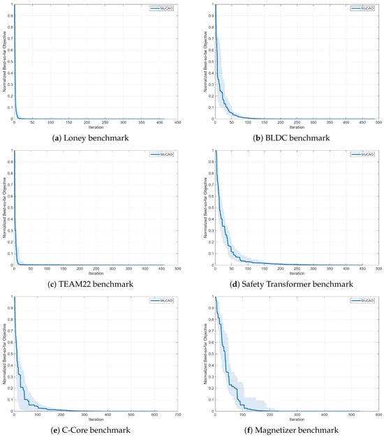
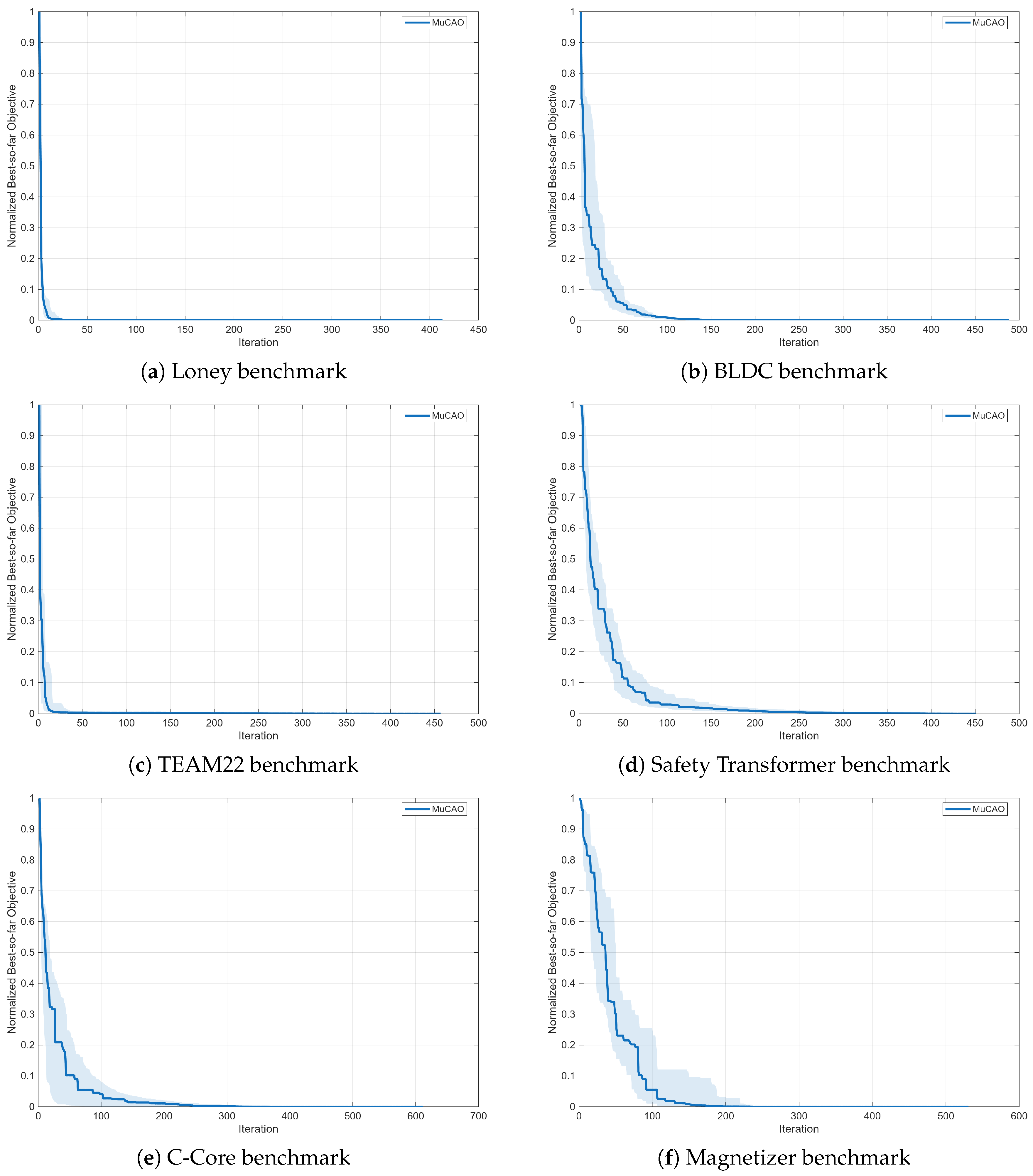
Figure 11 illustrates the normalized convergence profiles of MuCAO over the six benchmark problems. In each case, the solid curve represents the median normalized best-so-far objective value over the independent runs, while the shaded region denotes the interquartile range, thus reflecting the variability of the search process. Overall, the figures confirm that MuCAO exhibits a fast convergence rate, a stable optimization trajectory, and a gradual reduction in run-to-run variability as the search progresses.

Figure 11. Convergence curves for the MuCAO algorithms for all six benchmarks.

For the Loney benchmark, MuCAO shows a rapid initial decrease in the normalized objective value, indicating strong early exploration followed by efficient exploitation. Although the variability is relatively noticeable during the first iterations, the shaded band shrinks quickly, showing that different runs progressively agree on a similar search direction and converge to nearly the same final region. This behavior suggests that MuCAO is both effective and repeatable on this problem.

For the BLDC case, MuCAO again demonstrates a strong descent at the beginning of the search, followed by a smoother refinement phase. The interquartile band is wider in the early stage than in the later stage, which indicates sensitivity to the random initial population at the start, but the variance becomes very small as the iterations proceed. This confirms that the algorithm can recover from different initial conditions and still converge robustly.

For the Safety Transformer benchmark, the convergence is especially fast and sharp. The normalized objective drops to values close to zero in a relatively small number of iterations, and the shaded band becomes very narrow very early. This indicates not only high convergence speed but also excellent consistency across runs. Hence, MuCAO appears particularly well-suited to this benchmark.

For the TEAM22 benchmark, the same general trend is observed, but with a slightly more gradual reduction than in the Safety Transformer case. The algorithm still reaches the near-optimal region quickly, while the spread across runs contracts steadily. This reveals a good balance between exploration and exploitation, with MuCAO maintaining stable progress without prolonged stagnation.

For the C-Core benchmark, MuCAO exhibits a slower but still monotonic convergence pattern compared with the easiest cases. The decline of the normalized objective is smoother and extends over a larger number of iterations, which may indicate a more challenging search landscape. Nevertheless, the trajectory remains stable, and the narrowing of the interquartile region confirms that the algorithm consistently approaches high-quality solutions.

For the Magnetizer benchmark, MuCAO converges very rapidly, similarly to the Safety Transformer case. The objective value falls sharply within the first few iterations, and the variability across runs diminishes quickly. This behavior highlights the strong robustness of MuCAO on this benchmark and indicates that the algorithm can efficiently identify promising regions of the search space very early in the optimization process.

Taken together, these convergence profiles demonstrate that MuCAO has three desirable characteristics. First, it achieves rapid initial improvement, which reflects strong global search capability. Second, it shows stable refinement in later iterations, meaning that once promising regions are found, the algorithm can exploit them effectively. Third, the decreasing width of the interquartile band across all benchmarks confirms good robustness and repeatability, since different independent runs tend to converge toward similar final solutions.

A notable observation is that the convergence speed is not identical across all benchmarks. Some problems, such as the Safety Transformer and Magnetizer, are solved very quickly, whereas others, such as Loney, BLDC, and C-core, require a longer refinement stage. This difference is expected because the benchmarks have different landscape characteristics, dimensionalities, and constraint structures. Even so, MuCAO maintains a consistent and well-behaved convergence trend in all cases, which supports its suitability as a reliable optimizer for diverse electromagnetic design problems.

Overall, the results indicate that metaheuristic performance is highly benchmark-dependent due to differences in model type, dimensionality, and constraint complexity; however, unlike several algorithms that achieved first place only on specific cases, the proposed MuCAO demonstrated the most balanced and robust behavior across all six benchmarks, consistently remaining among the top performers with rankings between 2nd and 6th place. This stability suggests that MuCAO is less sensitive to problem-specific characteristics and is therefore well suited for diverse electromagnetic design tasks. In addition, while most modern metaheuristics outperformed the majority of the reference methods, with DE being the only classical algorithm that remained strongly competitive, the runtime analysis showed that computational cost varies significantly between analytical and FEM-based benchmarks. Accordingly, optimizer selection should consider not only solution quality but also robustness and computational efficiency, and from this perspective MuCAO offers a particularly attractive overall trade-off.

Sensitivity Study

In the description of MuCAO, two weights, $w_1$ and $w_2$, were introduced in Equation (4) to control the relative influence of the average-performance and best-performance terms, respectively. In the main study, equal weights were adopted, i.e., $w_1=w_2=0.5$. In this section, the effect of varying these two weights is investigated to assess their influence on the overall performance of the proposed algorithm. The corresponding results are reported in Table 17.

Table 17. Scores and ranks of MuCAO variants and the tested algorithms.

Algorithm	S1 *	R1 *	S2	R2	S3	R3	S4	R4	S5	R5	S6	R6	Score	Rank
MuCAO	9820.5	3	9603.5	2	10,438.5	2	9664	2	9283	3	7834.5	6	56,644	1
WSO	11,391	1	7030	9	10,590	1	10,481.5	1	7619	9	7215	11	54,326.5	2
MuCAO1 *	9820.5	4	9603.5	3	10,438.5	3	9664	3	6898	11	7834.5	7	54,259	3
MuCAO2 *	9820.5	5	9603.5	4	10,438.5	4	9597	4	6898	12	7834.5	8	54,192	4
MuCAO3 *	9434.5	6	9586.5	5	10,136.5	5	9456.5	6	7161	10	7950.5	5	53,725.5	5
TDO	8598	7	10,637	1	5635	13	7827.5	8	11,697	1	8923	3	53,317.5	6
AHA	8098	8	6729	11	10,038	6	9466.5	5	5325	13	7374	9	47,030.5	7
DE	11,107	2	6338	12	5562	14	8910.5	7	9211.5	4	4310	17	45,439	8
POA	6088	11	8444	6	6839	9	7225.5	11	8949	6	6932	12	44,477.5	9
TTA	5838	12	3357	17	7295	7	7232.5	10	8093	8	10,062	1	41,877.5	10
MVPA	7233	9	6986	10	5046	15	4553.5	15	11,198	2	3828	18	38,844.5	11
HGS	5423	13	5915	14	2730	19	4271.5	17	9067	5	9075	2	36,481.5	12
AFT	6495	10	4750	15	6951	8	7720.5	9	4169	14	4498	16	34,583.5	13
GEO	4858	14	6109	13	6449	11	5178.5	13	4155	16	7272	10	34,021.5	14
ZOA	4091	16	8341	7	3054	17	4792.5	14	4158	15	5763	13	30,199.5	15
GWO	2823	18	3920	16	6839	10	4533.5	16	3475	17	8092	4	29,682.5	16
PSO	4455	15	7056	8	2829	18	2687.5	18	8454.5	7	3248	19	28,730	17
BBO	3503	17	2576	19	5014	16	6250	12	2014	18	4938	15	24,295	18
SSA	2030	19	3237	18	5818	12	2588.5	19	1280	19	5196	14	20,149.5	19
RSO	659	20	563	20	390	20	913.5	20	612	20	608	20	3745.5	20
TLBO	20	21	122	21	322	21	338.5	21	13	21	33	21	848.5	21

* $S_i$ = Score on function i, $R_i$ = Rank on function i, MuCAO1 = MuCAO ($w_1$ = 0.25, $w_2$ = 0.75), MuCAO2 = MuCAO ($w_1$ = 0.75, $w_2$ = 0.25) and MuCAO3 = MuCAO ($w_1$ = 1, $w_2$ = 0).

It can be observed from Table 17 that the MuCAO configuration with equal weights achieves the best overall performance, obtaining the highest final score of 56,644 and ranking first among all compared approaches. Moving the balance towards the average-performance terms ($w_1=0.75$ and $w_2=0.25$) leads to a slightly reduced final score of 54,192, ranking fourth overall. Similarly, when more emphasis is given to the best-performing term, i.e., $w_1=0.25$ and $w_2=0.75$, the method achieves a final score of 54,259, ranking third. Considering only the average-performance term ($w_1=1$ and $w_2=0$) decreases the final score to 53,725.5, ranking fifth. These results indicate that both performance indicators play important and complementary roles in the adaptive selection mechanism. In particular, using only one term or overemphasizing one criterion at the expense of the other leads to a reduction in the overall effectiveness of the method. Therefore, the results confirm that the balanced setting $w_1=w_2=0.5$ provides the most suitable trade-off between average historical behavior and best-achieved performance, resulting in the strongest and most stable overall performance of MuCAO.

Another sensitivity analysis was conducted to investigate the influence of the number of constituent algorithms used to construct MuCAO. In the main configuration of the proposed method, MuCAO is formed by combining three algorithms, namely WSO, TDO, and AHA. To further examine the effect of this choice, an additional variant, denoted as MuCAO5, was also considered, in which four algorithms, WSO, TDO, AHA, and DE, were combined. The corresponding results are reported in Table 18.

Table 18. Scores and ranks obtained by MuCAO variants and the compared algorithms.

Algorithm	S1 *	R1 *	S2	R2	S3	R3	S4	R4	S5	R5	S6	R6	Score	Rank
MuCAO	9201	3	9014	2	9819	2	8910.5	3	8203.5	4	7209.5	6	52,357.5	1
MuCAO5 *	9031	4	8424	3	9270	4	9577.5	1	8203.5	5	7209.5	7	51,715.5	2
WSO	10,409	1	6900	6	9905	1	9574.5	2	6725	10	6677	9	50,190.5	3
TDO	8270	5	9872	1	5659	10	7493.5	6	10,310	1	8145	3	49,749.5	4
AHA	7864	6	6597	9	9578	3	8801.5	4	4864	11	6818	8	44,522.5	5
DE	10,309	2	6260	10	5468	11	8222.5	5	8341.5	3	3997	15	42,598	6
POA	6024	8	8022	4	6745	7	7006.5	8	7839	7	6410	10	42,046.5	7
TTA	5859	10	3348	15	7246	5	6998.5	9	7120	9	9108	1	39,679.5	8
MVPA	7061	7	6750	8	5001	13	4531.5	12	9735	2	3602	16	36,680.5	9
HGS	5415	11	5656	11	2740	17	4246.5	14	7907	6	8243	2	34,207.5	10
AFT	6017	9	4446	12	6617	8	7152.5	7	3605	13	4112	14	31,949.5	11
ZOA	4092	13	7932	5	3068	15	4752.5	11	3917	12	5379	11	29,140.5	12
GWO	2823	15	3774	14	6828	6	4527.5	13	3314	14	7438	5	28,704.5	13
PSO	4415	12	6760	7	2825	16	2685.5	15	7360.5	8	3138	17	27,184	14
BBO	3503	14	2571	17	5034	12	5625	10	1984	16	4656	13	23,373	15
GEO	1196	17	4197	13	3650	14	1701.5	17	3126	15	7717	4	21,587.5	16
SSA	2030	16	3145	16	5810	9	2588.5	16	1280	17	4930	12	19,783.5	17
RSO	659	18	563	18	390	18	913.5	18	612	18	608	18	3745.5	18
TLBO	20	19	122	19	322	19	338.5	19	13	19	33	19	848.5	19

* $S_i$ = Score on function i, $R_i$ = Rank on function i, MuCAO5 = MuCAO using 4 algorithms.

It can be observed from Table 18 that both hybrid configurations outperform all standalone algorithms in terms of the overall cumulative score, with MuCAO (using three algorithms) achieving the best final score of 52,357.5 and ranking first overall, while MuCAO5 (using four algorithms) attains a slightly lower score of 51,715.5 and ranks second. This result indicates that increasing the number of constituent algorithms does not necessarily lead to improved overall performance. Although the inclusion of an additional strong algorithm may enrich the pool of candidate search strategies, it may also introduce more variability into the adaptive selection process and reduce the coherence of the hybrid behavior.

These observations demonstrate that the performance of the interaction among the constituent algorithms within the adaptive selection framework is important, in addition to the quality of the individual algorithm. This means that adding more algorithms could improve search diversity, but at the expense of the contributions of the most suitable algorithms. Hence, for the considered benchmark set, the results support the use of three constituent algorithms as the most suitable configuration for MuCAO.

5.2. Application #2: Sidelobe Level Reduction in a Circular Antenna Array

For performance validation, a second application is used in this paper. In this application, the performance of the developed MuCAO is compared against the comparing algorithms to check if the conclusions drawn in the previous section are valid. Antenna arrays play a central role in many modern wireless systems, including radar, mobile communications, military applications, and satellite communications [47]. Among the different array geometries, the circular antenna array (CAA) is an important configuration in which N isotropic elements are uniformly distributed along a circle of radius r in the x–y plane. In this application, the developed MuCAO is applied to solve a real-life EMD optimization problem, namely the reduction of the sidelobe level (SLL) in a CAA.

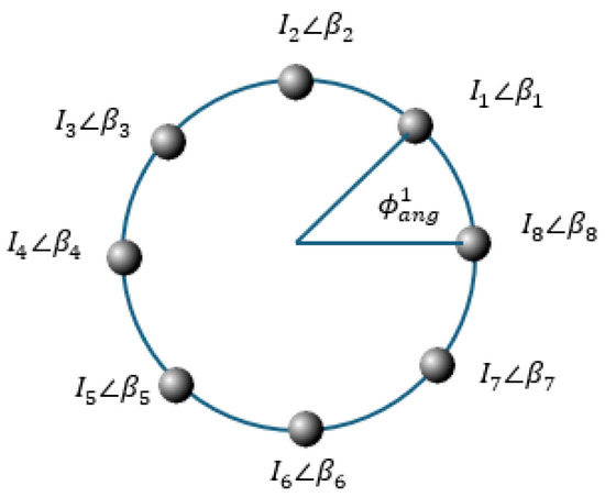
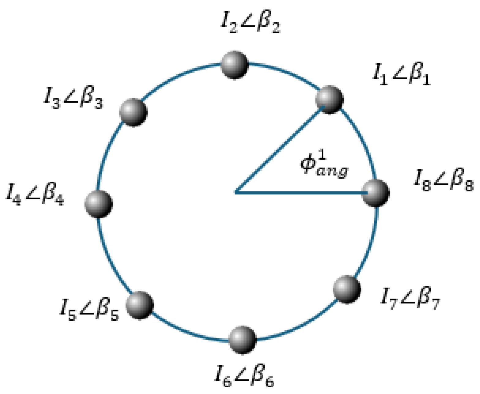
Figure 12 shows the geometry of the investigated CAA consisting of N elements. The corresponding array factor $AF\left(\varphi \right)$ is expressed as follows:

$$AF\left(\varphi \right)={\displaystyle \sum _{n=1}^N}{I}_{n}exp\left\{j\left[kr\left(cos(\varphi -{\varphi }_n)-cos({\varphi }_0-{\varphi }_n)\right)+{\beta }_n\right]\right\},$$

(40)

where $I_n$ is the current excitation of the nth element, r is the radius of the circular array, k is the wave number, and

$${\varphi }_n={\displaystyle \frac{2\pi (n-1)}{N}}$$

(41)

is the angular position of the nth element. In addition, $\varphi$ is the observation angle, ${\varphi }_0$ is the direction of maximum radiation, and ${\beta }_n$ is the phase excitation of the nth element.

Figure 12. Configuration of a circular antenna array (CAA) with N elements uniformly distributed on a circle of radius r in the x–y plane [48].

The objective function used for the optimal design of the CAA with reduced SLL is expressed as follows [48]:

$$OF={\displaystyle \frac{\left|AR({\varphi }_{\mathrm{SLL}},I,\beta ,{\varphi }_0)\right|}{\left|AR({\varphi }_{max},I,\beta ,{\varphi }_0)\right|}}+\left|{\varphi }_0-{\varphi }_{\mathrm{des}}\right|,$$

(42)

where the first term aims to minimize the undesired sidelobes, with ${\varphi }_{\mathrm{SLL}}$ being the angle at which the maximum sidelobe occurs. The second aims to force the main beam maximum to remain close to the desired steering direction ${\varphi }_{\mathrm{des}}$.

Although the main objective in this application is to minimize SLL, other performance criteria may also be incorporated into the problem formulation. For instance, the half-power beam-width (HPBW) can be minimized to obtain a narrower beam, while the dynamic range ratio (DRR) may also be considered depending on the design requirements [48]. This may be considered in future studies as a multi-objective optimization problem.

The design variables for the CAA optimal design problem are the current amplitudes $I_n\in [0.2,1] \mathrm{A}$ and phase excitations ${\beta }_n\in [-180°,180°]$ of the array elements.

In this study, a CAA with 12 elements is considered, and the desired beam direction is set to ${\varphi }_{\mathrm{des}}=180°$. Consequently, the resulting optimization problem involves 24 design variables. Furthermore, the parameters used for this application, population size, maximum number of iterations, and maximum number of function evaluations, are the same as given in Section 5.1.

The obtained results for all the tested algorithms are shown in Table 19. This table shows that the MuCAO outperforms all the remaining algorithms with a total score of 9516. The WSO, TDO, and AHA are ranked 2nd, 3rd, and 4th, respectively. These results confirm the superiority of the developed approach.

Table 19. Optimal results of tested algorithms for the CAA.

Algorithm	Final Rank	Total Score	Best	Mean	Median	Standard Deviation	Worst
MuCAO	1	9516	−21.282	−18.955	−19.824	2.474	−13.424
WSO	2	9069	−21.006	−18.216	−18.498	1.780	−14.959
TDO	3	9013	−20.340	−18.103	−18.008	0.907	−16.842
AHA	4	8670	−21.184	−17.417	−17.927	2.501	−13.170
AFT	5	6795	−21.428	−17.221	−18.837	4.059	−10.870
POA	6	6690	−19.823	−14.168	−13.247	1.921	−12.146
BBO	7	6457	−18.304	−13.954	−13.698	1.809	−10.767
TTA	8	5717	−19.819	−13.799	−12.220	3.305	−10.864
GWO	9	5390	−18.046	−13.369	−12.908	2.727	−10.213
GEO	10	4851	−12.959	−12.175	−12.308	0.482	−10.747
ZOA	11	4553	−17.054	−12.298	−11.968	1.712	−10.086
DE	12	4099	−17.083	−11.807	−12.129	1.347	−10.358
MVPA	13	3805	−17.037	−11.877	−10.857	2.267	−9.318
HGS	14	3550	−15.782	−11.480	−11.018	1.334	−9.920
SSA	15	3483	−15.406	−11.460	−11.198	1.467	−9.919
PSO	16	1937	−12.783	−10.100	−10.001	0.980	−8.921
RSO	17	588	−8.440	−8.026	−7.987	0.147	−7.780
TLBO	18	37	−8.264	−7.484	−7.369	0.296	−7.163

Finally, as described earlier, the top three algorithms are selected based on their overall cumulative performance on selected EMD benchmarks, which are then combined following some probabilistic strategy. An alternative approach could be to individually select the top-performing algorithms for each benchmark before combining them to form benchmark-specific versions of MuCAO. The proposed alternative approach is a subject for future studies.

6. Conclusions

This work started with a performance analysis of selected modern metaheuristic algorithms for the optimal design of EMDs. Subsequently, a new hybrid optimization technique called MuCAO was developed by adaptively combining the top three performing metaheuristics from a pool. Both analytical and FEM-based benchmarks were used to evaluate the performance of the proposed algorithm.

MuCAO achieved the highest cumulative performance score, outperforming all the compared algorithms across all benchmarks. MuCAO achieved a narrow ranking variation (from 2nd to 6th), demonstrating its robustness. The results of the study also showed that MuCAO had a good balance between solution quality and computational burden. Individual algorithms such as WSO and TDO had good performance, ranking second and third, respectively. However, unlike MuCAO, which demonstrated consistent performance across various benchmarks, both individual algorithms demonstrated variability in performance across different benchmarks.

The design of MuCAO proposed here is based on global performance across all benchmarks. This could limit the applicability of the technique to diverse problem types. Hence, the method could be improved by adapting the content algorithms to specific problems. Furthermore, another opportunity for improvement is in the number of combined algorithms. Rather than arbitrarily fixing the number as done in this work, a systematic approach could be developed for deciding the number of constituent algorithms.

Therefore, future work will consider adaptive strategies for combining the algorithms based on some criteria, such as performance on specific benchmarks, while dynamically adjusting the number of algorithms during the optimization process. The automatic selection and tuning of the method based on problem signature, and the use of alternative models that are less computationally demanding for the FEM-based problems, present plausible research directions.

With the extensions highlighted above and other possible refinements, MuCAO presents a promising technique for EMD optimization and other complex engineering design problems.

References

- Slim, M.; Rokbani, N.; Terres, M.A.; Watelain, E.; Ben Khelifa, M.M. Optimization of Soft Actuator Geometry and Material Modeling Using Metaheuristic Algorithms. Actuators 2025, 14, 520. [Google Scholar] [CrossRef] [Scilit]
- Zheng, Y.; Sun, R.; Liu, Y.; Wang, Y.; Song, R.; Li, Y. A Hybridization Grey Wolf Optimizer to Identify Parameters of Helical Hydraulic Rotary Actuator. Actuators 2023, 12, 220. [Google Scholar] [CrossRef] [Scilit]
- Ji, T.K.; Baek, S.W. Optimal Design of a Coaxial Magnetic Gear Considering Thermal Demagnetization and Structural Robustness for Torque Density Enhancement. Actuators 2026, 15, 59. [Google Scholar] [CrossRef] [Scilit]
- Đurić, M.; Selak, L.; Bračun, D. Hybrid Design Optimization Methodology for Electromechanical Linear Actuators in Automotive LED Headlights. Actuators 2025, 14, 465. [Google Scholar] [CrossRef] [Scilit]
- Ding, Z.; Bi, J.; Wu, S.; Lv, C.; Chi, M.; Deng, Z. Design and Investigation of Powertrain with In-Wheel Motor for Permanent Magnet Electrodynamic Suspension Maglev Car. Actuators 2026, 15, 58. [Google Scholar] [CrossRef] [Scilit]
- Oh, S.M.; Akatsu, K.; Lee, D.W.; Lee, H.J. On the Iron Loss Reduction Design Improvement of an Axial Flux Permanent Magnet Motor. Actuators 2025, 14, 595. [Google Scholar] [CrossRef] [Scilit]
- Peng, Z.; Zheng, Z.; Yang, S.; Zhao, X.; Yu, X.; Han, D. Design and Optimization of a Pneumatic Microvalve with Symmetric Magnetic Yoke and Permanent Magnet Assistance. Actuators 2025, 14, 388. [Google Scholar] [CrossRef] [Scilit]
- Uler, G.; Mohammed, O. Utilizing genetic algorithms for the optimal design of electromagnetic devices. IEEE Trans. Magn. 1994, 30, 4296–4298. [Google Scholar] [CrossRef] [Scilit]
- Fanni, A.; Manunza, A.; Marchesi, M.; Pilo, F. Tabu search metaheuristics for global optimization of electromagnetic problems. IEEE Trans. Magn. 1998, 34, 2956–2959. [Google Scholar] [CrossRef] [Scilit]
- Ciuprina, G.; Ioan, D.; Munteanu, I. Use of intelligent-particle swarm optimization in electromagnetics. IEEE Trans. Magn. 2002, 38, 1037–1040. [Google Scholar] [CrossRef] [Scilit]
- Campelo, F.; Guimaraes, F.G.; Igarashi, H.; Ramirez, J.A. A clonal selection algorithm for optimization in electromagnetics. IEEE Trans. Magn. 2005, 41, 1736–1739. [Google Scholar] [CrossRef] [Scilit]
- Alfonzetti, S.; Dilettoso, E.; Salerno, N. Simulated annealing with restarts for the optimization of electromagnetic devices. IEEE Trans. Magn. 2006, 42, 1115–1118. [Google Scholar] [CrossRef] [Scilit]
- Coelho, L.D.S.; Alotto, P. Particle swarm optimization combined with normative knowledge applied to Loney’s solenoid design. COMPEL Int. J. Comput. Math. Electr. Electron. Eng. 2009, 28, 1155–1161. [Google Scholar] [CrossRef] [Scilit]
- Zhang, X.; Zhang, X.; Yuen, S.Y.; Ho, S.L.; Fu, W.N. An improved artificial bee colony algorithm for optimal design of electromagnetic devices. IEEE Trans. Magn. 2013, 49, 4811–4816. [Google Scholar] [CrossRef] [Scilit]
- Bouchekara, H. Optimal design of electromagnetic devices using a black-Hole-Based optimization technique. IEEE Trans. Magn. 2013, 49, 5709–5714. [Google Scholar] [CrossRef] [Scilit]
- Bouchekara, H. Electromagnetic Device Optimization Based on Electromagnetism-Like Mechanism. Appl. Comput. Electromagn. Soc. J. 2013, 28, 241–248. [Google Scholar]
- Coco, S.; Laudani, A.; Fulginei, F.; Salvini, A. Bacterial chemotaxis shape optimization of electromagnetic devices. Inverse Probl. Sci. Eng. 2014, 22, 910–923. [Google Scholar] [CrossRef] [Scilit]
- Bouchekara, H.; Nahas, M. Optimization of electromagnetics problems using an improved teaching-learning-based-optimization technique. Appl. Comput. Electromagn. Soc. J. 2015, 30, 1341–1347. [Google Scholar]
- Klein, C.E.; Segundo, E.H.V.; Mariani, V.C.; dos S. Coelho, L. Modified Social-Spider Optimization Algorithm Applied to Electromagnetic Optimization. IEEE Trans. Magn. 2016, 52, 7208304. [Google Scholar] [CrossRef] [Scilit]
- Alb, M.; Alotto, P.; Magele, C.; Renhart, W.; Preis, K.; Trapp, B. Firefly Algorithm for Finding Optimal Shapes of Electromagnetic Devices. IEEE Trans. Magn. 2016, 52, 7002504. [Google Scholar] [CrossRef] [Scilit]
- Ho, S.L.; Yang, S.; Bai, Y.; Li, Y. A Wind Driven Optimization-Based Methodology for Robust Optimizations of Electromagnetic Devices under Interval Uncertainty. IEEE Trans. Magn. 2017, 53, 7001204. [Google Scholar] [CrossRef] [Scilit]
- Bouchekara, H.R.E.H.; Nahas, M.; Kaouach, H.M. Optimal Design of Electromagnetic Devices Using the League Championship Algorithm. Appl. Comput. Electromagn. Soc. J. 2017, 32, 484–490. [Google Scholar]
- Yang, W.; Ho, S.L.; Yang, S. An efficient direct search methodology for robust optimization of electromagnetic devices. IEEE Trans. Magn. 2018, 54, 7001004. [Google Scholar] [CrossRef] [Scilit]
- Ciuprina, G.; Lup, S.; Duca, I.H.A. ACOR Algorithm’s Efficiency for Electromagnetic Optimization Benchmark Problems. In Proceedings of the 11th International Symposium on Advanced Topics in Electrical Engineering, Bucharest, Romania, 28–30 March 2019. [Google Scholar]
- Abedinifar, M.; Ertugrul, S.; Tayyar, G.T. Design optimization of a solenoid actuator using particle swarm optimization algorithm with multiple objectives. Adv. Mech. Eng. 2022, 14, 1–12. [Google Scholar] [CrossRef] [Scilit]
- Feng, T.; Deng, S.; Duan, Q.; Mao, Y. Application of Local Search Particle Swarm Optimization Based on the Beetle Antennae Search Algorithm in Parameter Optimization. Actuators 2024, 13, 270. [Google Scholar] [CrossRef] [Scilit]
- Mussetta, M.; Grimaccia, F.; Zich, R. Comparison of different optimization techniques in the design of electromagnetic devices. In Proceedings of the 2012 IEEE Congress on Evolutionary Computation, Brisbane, QLD, Australia, 10–15 June 2012; pp. 1–6. [Google Scholar] [CrossRef] [Scilit]
- Bechari, R.E.; Brisset, S.; Clenet, S.; Guyomarch, F.; Mipo, J.C.; Clénet, S.; Mipo, J.C. Comparison of Approaches for Optimization of Electromagnetic Devices using Finite Element Method. In Proceedings of the Compumag, Paris, France, 15–19 July 2019. [Google Scholar]
- Braik, M.; Ryalat, M.H.; Al-Zoubi, H. A novel meta-heuristic algorithm for solving numerical optimization problems: Ali Baba and the forty thieves. Neural Comput. Appl. 2022, 34, 409–455. [Google Scholar] [CrossRef] [Scilit]
- Mohammadi-Balani, A.; Nayeri, M.D.; Azar, A.; Taghizadeh-Yazdi, M. Golden eagle optimizer: A nature-inspired metaheuristic algorithm. Comput. Ind. Eng. 2021, 152, 107050. [Google Scholar] [CrossRef] [Scilit]
- Yang, Y.; Chen, H.; Heidari, A.A.; Gandomi, A.H. Hunger games search: Visions, conception, implementation, deep analysis, perspectives, and towards performance shifts. Expert Syst. Appl. 2021, 177, 114864. [Google Scholar] [CrossRef] [Scilit]
- Dhiman, G.; Garg, M.; Nagar, A.; Kumar, V.; Dehghani, M. A novel algorithm for global optimization: Rat Swarm Optimizer. J. Ambient. Intell. Humaniz. Comput. 2021, 12, 8457–8482. [Google Scholar] [CrossRef] [Scilit]
- Fadzil, M.F.F.M. Tiki-taka algorithm: A novel metaheuristic inspired by football playing style. Eng. Comput. 2021, 38, 313–343. [Google Scholar] [CrossRef] [Scilit]
- Trojovský, P.; Dehghani, M. Pelican Optimization Algorithm: A Novel Nature-Inspired Algorithm for Engineering Applications. Sensors 2022, 22, 855. [Google Scholar] [CrossRef] [Scilit]
- Dehghani, M.; Hubalovsky, S.; Trojovsky, P. Tasmanian Devil Optimization: A New Bio-Inspired Optimization Algorithm for Solving Optimization Algorithm. IEEE Access 2022, 10, 19599–19620. [Google Scholar] [CrossRef] [Scilit]
- Trojovska, E.; Dehghani, M.; Trojovsky, P. Zebra Optimization Algorithm: A New Bio-Inspired Optimization Algorithm for Solving Optimization Algorithm. IEEE Access 2022, 10, 49445–49473. [Google Scholar] [CrossRef] [Scilit]
- Zhao, W.; Wang, L.; Mirjalili, S. Artificial hummingbird algorithm: A new bio-inspired optimizer with its engineering applications. Comput. Methods Appl. Mech. Eng. 2022, 388, 114194. [Google Scholar] [CrossRef] [Scilit]
- Brisset, S.; Brochet, P. Analytical model for the optimal design of a brushless DC wheel motor. COMPEL Int. J. Comput. Math. Electr. Electron. Eng. 2005, 24, 829–848. [Google Scholar] [CrossRef] [Scilit]
- Barba, P.D.; Gottvald, A.; Savini, A. Global optimization of Loney’s Solenoid a benchmark problem. Int. J. Electromagn. Mech. 1995, 6, 273–276. [Google Scholar] [CrossRef] [Scilit]
- Coelho, L.D.S.; Alotto, P. Global Optimization of Electromagnetic Devices Using an Exponential Quantum-Behaved Particle Swarm Optimizer. IEEE Trans. Magn. 2008, 44, 1074–1077. [Google Scholar] [CrossRef] [Scilit]
- Alotto, P.; Baumgartner, U.; Freschi, F.; Jaindl, M.; Kostinger, A.; Magele, C.; Repetto, W. SMES optimization Benchmark: TEAM workshop problem 22. In Proceedings of the COMPUMAG TEAM Workshop, Okayama, Japan, 14–16 September 2008; pp. 1–4. [Google Scholar]
- Tran, T.; Brisset, S.; Brochet, P. A benchmark for multi-objective, multi-level and combinatorial optimizations of a safety isolating transformer. In Proceedings of the COMPUMAG, Aachen, Germany, 24–28 June 2007; pp. 167–168. [Google Scholar]
- Soares, J.; Lezama, F.; Vale, Z.; Brisset, S.; François, B. Safety Isolating Transformer Design using HyDE-DF algorithm. In Proceedings of the 2020 IEEE Congress on Evolutionary Computation (CEC), Glasgow, UK, 19–24 July 2020; pp. 1–7. [Google Scholar] [CrossRef] [Scilit]
- Farina, M.; Sykulski, J.K. Comparative study of evolution strategies combined with approximation techniques for practical electromagnetic optimization problems. IEEE Trans. Magn. 2001, 37, 3216–3220. [Google Scholar] [CrossRef]
- Sykulski, J.K. Reducing computational effort in field optimisation problems. COMPEL Int. J. Comput. Math. Electr. Electron. Eng. 2004, 23, 159–172. [Google Scholar] [CrossRef] [Scilit]
- Mohamed, A.W.; Hadi, A.A.; Mohamed, A.K.; Agrawal, P.; Kumar, A.; Suganthan, P. Problem Definitions and Evaluation Criteria for the CEC 2021 Special Session and Competition on Single Objective Bound Constrained Numerical Optimization; Nanyang Technological University Singapore: Singapore, 2020. [Google Scholar]
- Dib, N. Design of planar concentric circular antenna arrays with reduced side lobe level using symbiotic organisms search. Neural Comput. Appl. 2018, 30, 3859–3868. [Google Scholar] [CrossRef] [Scilit]
- Bouchekara, H.R.E.H. Electric Charged Particles Optimization and its application to the optimal design of a circular antenna array. Artif. Intell. Rev. 2021, 54, 1767–1802. [Google Scholar] [CrossRef] [Scilit]
Disclaimer/Publisher’s Note: The statements, opinions and data contained in all publications are solely those of the individual author(s) and contributor(s) and not of MDPI and/or the editor(s). MDPI and/or the editor(s) disclaim responsibility for any injury to people or property resulting from any ideas, methods, instructions or products referred to in the content. |
© 2026 by the authors. Licensee MDPI, Basel, Switzerland. This article is an open access article distributed under the terms and conditions of the Creative Commons Attribution (CC BY) license.