


Abstract
This paper presents a hierarchical control architecture for high-precision trajectory tracking of a car-like mobile robot (CLMB) operating under external disturbances arising from normal and tangential wheel forces. The proposed solution addresses the critical challenge of simultaneously rejecting disturbances and accurately following a predefined path at a determined cruise velocity. Since the vehicle is equipped with an electronic differential at the low level, a nonlinear dynamic control (NDC) scheme is implemented to regulate the speed in each wheel. This controller actively estimates and compensates for differential traction losses and other lumped disturbances in real time, ensuring robust wheel velocity tracking across varying terrain conditions. The compensated system is then governed by a high-level frugal model predictive controller (FMPC) that leverages a dynamic vehicle model to compute optimal steering and velocity commands, thereby minimizing future trajectory-tracking errors. To achieve a precise and reliable state estimation necessary for feedback control, an Extended Kalman Filter (EKF) is designed to fuse high-frequency data from wheel encoders with absolute pose measurements from a motion capture system, mitigating the drift inherent in odometry alone. Experimental results on a physical robotic platform demonstrate tracking accuracy and robust disturbance rejection under different operating conditions.
1. Introduction
1.1. Preliminaries
Mobile robotics has undergone an unprecedented evolution, driven by the need to automate tasks in sectors as diverse as logistics, precision agriculture, and autonomous transportation [1,2,3,4]. However, achieving full autonomy remains an open challenge, constrained by the vehicles’ ability to perceive, localize, and navigate safely in dynamic and uncertain environments [5,6]. This challenge extends beyond general mobile robotics into the automotive sector, specifically regarding autonomous electric vehicles [7,8,9]. In this context, vehicles with car-like kinematic configurations represent a critical case study due to their widespread adoption in industry and their non-holonomic constraints, which introduce additional complexity to the planning and execution of maneuvers [10,11,12].
Since its initial formulations, the problem of optimal estimation in dynamic systems has been addressed through recursive models that combine sensor data with system predictions. The seminal work of Kalman [13] established the foundation for the filter that bears his name, offering an optimal solution for linear systems with Gaussian noise, characterized by its computational efficiency and recursive nature, Subsequently, this concept has been extended to accommodate the complexities of nonlinear systems [14], this is fundamental for modern robotics where sensor models and vehicle kinematics rarely follow linear assumptions. The recent literature identifies that robust navigation in complex scenarios—where global positioning signals are often unreliable—demands the integration of multisensory architectures capable of mitigating uncertainty [2,6,10]. In this field, sensor data fusion through the Kalman Filter (KF) and its extensions for nonlinear systems, such as the Extended Kalman Filter (EKF), has consolidated as the de facto standard for ensuring consistent state estimation and precise obstacle avoidance [1,3]. Current studies demonstrate that the combination of trilateral localization techniques with advanced filtering allows mobile robots to operate successfully even in chaotic and semi-open environments, laying the groundwork for next-generation industrial and service applications [15]. Alternatively, for outdoor environments, Ref. [16] presents a method to combine Global Navigation Satellite System (GNSS) and BeiDou Navigation Satellite System (BeiDou) data with a low-cost Inertial Measurement Unit (IMU) sensor using an EKF to enhance positioning accuracy. Integrating multiple GNSS systems with a Micro–Electro-Mechanical System Inertial Measurement Unit (MEMS IMU) facilitates achieving centimeter-level precision, which is essential for precision agriculture, autonomous vehicles, and surveying. Recently, the literature has explored the use of deep learning techniques, such as Recurrent Neural Networks (RNNs), to model complex dynamic uncertainties that linear filters fail to capture [17]; however, Wang et al. [18] present a comparative study demonstrating that the EKF maintains a critical superiority in terms of computational efficiency and predictability for real-time vehicle control. In contrast, AI-based approaches [19] often require significant computational load and large volumes of training data.
Once the positioning problem has been resolved, the next challenge consists of precise trajectory tracking. The robot is subject to non-holonomic constraints, and the robotic system is nonlinear and underactuated. These characteristics increase the control design challenge [20]. Various control strategies have been developed to solve this problem, ranging from classical controllers and geometric algorithms to optimal and robust controllers, and, recently, the incorporation of artificial intelligence [21]. In [22,23], control structures based on PID are proposed to achieve trajectory tracking; however, the optimality of the control signal is a factor to consider. In [24], an LQR controller is proposed that better adapts to the lateral tracking control problem of intelligent vehicles under complex operating conditions. The robustness of the control against external perturbations or unmodeled dynamics is crucial in practical implementations; based on that assumption, Ref. [25] presents a backstepping second-order sliding mode control so that the kinematic error states, after a nonlinear transformation, tend to zero in finite time. Given the difficulty of establishing a precise vehicle model, the perturbations to which it may be subjected, and the dynamics it undergoes, control alternatives based on observers [26,27,28,29,30] and the use of AI [31,32]) have emerged. Recently, Model Predictive Control (MPC) has emerged as a robust solution thanks to its ability to anticipate future states and explicitly manage state and input constraints [33]. Various hybrid control schemes based on MPC have been developed [34,35,36] to address deficiencies in the MPC model. Nevertheless, a trade-off exists between the use of nonlinear models (NMPC), which offer a more realistic representation but incur high computational cost and optimization complexity, and linearized models, which facilitate real-time implementation and guaranty more efficient convergence in practical applications [37].
To optimize the implementation of Model Predictive Control (MPC), this work utilizes the concept of feedback linearization, which involves a change in the coordinates applied to the kinematic model of a car-like robot. This approach has been previously explored in the development of various control strategies [38,39,40,41,42]. By employing this method, the system can be simplified to a structure consisting of two simple integrators for the trajectory coordinates in the plane [12,43,44]. This decoupled model enables the MPC optimizer to address the control problem [45]. Subsequently, the calculated control signals are transformed into the vehicle’s physical variables using the inverse coordinate transformation, ensuring correspondence between kinematic prediction and execution.
Translating trajectory control signals into traction system involves careful consideration of the vehicle’s mechanics, such as whether it is two-wheel or four-wheel drive [46]. For example, rear-wheel differential systems [47] use Ackermann–Jeantand geometry to determine the reference velocities for each motor. This electronic differential maintains a consistent velocity difference between the inner and outer wheels during turns, helping prevent slippage and maintaining motion integrity. In terms of alternative methods, Ref. [48] proposes a mechanical system of coupled pedals that enables independent control of wheel speed. In [49], a differential torque control method is proposed; however, the complexity of modeling both the vehicle and the motor remains a significant challenge. To tackle this issue, the work presented in [50] introduces a control law that focuses on regulation error. This approach utilizes low-pass and high-pass filtering of the control signal to enhance performance.
Effective displacement towards target setpoints within a trajectory-tracking framework is achieved by coordinating steering control with the regulation of traction motor angular velocity. To improve system performance in the face of environmental uncertainties, a disturbance estimator can be integrated into the control law [51,52,53,54,55]. This integrated approach enhances robustness, ensuring stable and precise trajectory tracking even under challenging real-world operating conditions.
The experimental phase and validation of theoretical results are crucial in research. The engineering challenge involves developing and effectively integrating systems to close the gap between theory and practice. In the field of mobile robotics, Ref. [56] outlines the fabrication process for various mobile robots platforms. Additionally, Ref. [57] presents an integrated framework for indoor localization along with experimental validation using an autonomous ADAS-based model car. This vehicle determines its global position by merging data from fiducial markers, inertial sensors, and wheel odometry. Moreover, Ref. [58] introduces a testbed designed to evaluate control strategies under outdoor conditions, offering a cost-efficient and repeatable alternative to full-scale vehicle testing.
1.2. Contribution
The primary contribution of this work is the solution’s frugality, which transforms a complex problem—specifically, the trajectory tracking of a car-like mobile robot equipped with an electronic differential—into a modular system incorporating a multi-level hierarchical control scheme. This approach presents a well-considered reformulation that enables the resolution of a nonlinear tracking problem while maintaining the computational efficiency of the quadratic programming (QP) problem associated with linear Model Predictive Control (MPC). Additionally, to decrease the number of decision variables in the QP-problem, a control parameterization method is utilized. This choice decreases the complexity of the optimization problem without compromising the performance of the closed-loop system.
The following list summarizes our contributions:
- Hierarchical integration: We present a modular framework that combines an Extended Kalman Filter (EKF), a Frugal Model Predictive Control (FMPC), and an electronic differential. In this framework, the velocity of each wheel is independently regulated by a nonlinear dynamic control law capable of addressing model uncertainties and external disturbances.
- Nonlinear-to-linear structure via coordinate transformation: Although the kinematics of the car-like mobile robot are governed by a nonlinear model with non-holonomic constraints, we propose controlling the position of a virtual point (“nose”) located at a distance p along the line that is normal to the wheel axis. The kinematics associated with the “nose” position are holonomic, so we can apply a coordinate transformation that effectively decouples the system into two first-order integrators. Controlling the nose position is practically relevant, as this location can accommodate a suite of sensors and a camera.
- MPC based on an integrator mode: Unlike conventional nonlinear MPC (NMPC) the predictive model used in the present work consists of two pure integrators. This transformation leads to a quadratic programming (QP) problem with minimal computational burden, retaining the advantages of linear MPC (e.g., convexity and efficiency) while handling the nonlinear system.
- Control parametrization: To reduce the number of decision variables in the quadratic programming (QP) problem, a reduced control parametrization is adopted. With such a choice, the optimization problem’s complexity is reduced without compromising the closed loop’s performance.
- Experimental validation: To experimentally validate the proposed strategy, a simple yet complete experimental platform is developed using: (1) open and standardized communication protocols, (2) a on-board embedded system to drive wheel angular velocities and direcction, and (3) a MATLAB-ROS (Robot Operating System) ground station.
- Realiability analysis: The reliability of the control strategy was assessed by evaluating its ability to track the desired trajectory, reject disturbances, and meet constraints related to both the state and control. Additionally, we examined the capability of the Extended Kalman Filter (EKF) to integrate relative measurements (odometry) and absolute measurements (position data obtained from motion capture) at various sampling times. Performance was quantified using three well-established indices: the Integral of the Squared Error (ISE), the Integral of the Absolute Error (IAE), and the Integral of Time-weighted Absolute Error (ITAE). The results highlight the effectiveness, reliability, and significance of the proposed strategy.
The remainder of this paper is organized as follows: Section 2 presents the mathematical preliminaries and the problem statement. Section 3 focuses on the control design and estimation design. Section 4, Section 5 and Section 6 describe the development of the experimental platform and its main components, as well as the corresponding results. Finally, Section 7 presents the conclusions.
2. Mathematical Preliminaries and Problem Statement
2.1. Car-like Mobile Robot
Consider a car-like mobile robot as shown in Figure 1. It is important to note the reduction in the geometric representation from four to two wheels (bicycle model): one for traction (rear wheel) and the other for direction (front wheel). To establish the mathematical equations for the kinematic model, the reference point for vehicle position is located at the midpoint of the rear axle. Finally, the kinematic bicycle model is defined as follows:
where is the longitudinal velocity of the vehicle, is the steering angle, and corresponds to the wheelbase. Furthermore, let us define the angular velocity of the frame with respect to by .
Figure 1.
Kinematic bicycle model for car-like mobile robot.
In trajectory-tracking control for a car-like mobile robot using the kinematics model, it is well known that the system’s control signals are the longitudinal velocity and the steering angle . From Figure 1 the front wheel angle can be defined as a function of and (vehicle’s angular velocity) in the form
In this work, the mobile robot configuration uses Ackermann steering and differential traction on the rear axle, i.e., the left and right wheels are coupled to independent electric motors. Let us define the notation for the angular velocity of each wheel as
Using this traction configuration, each wheel can rotate at a different speed without a mechanical differential; additionally, the tire torque can be controlled independently, providing greater stability during various maneuvers and under different road conditions. The longitudinal displacement velocity of the mobile robot is established as a function of the angular velocities of the wheels:
where r denotes the radius of the wheels of the mobile robot.
2.2. Electronic Differential Based on Ackermann Geometry
Based on the Ackermann steering geometry, we can derive the angular velocities of the inner and outer wheels for curved trajectories. This kinematic model is designed for low-speed operation and assumes that lateral forces and longitudinal tire slip can be neglected. As illustrated in Figure 2, the model relates the steering angles ( and ) to the radius of rotation (). This relationship allows us to determine the appropriate angular speeds ( and ) for the drive wheels.
Figure 2.
Ackermann geometry with electronic differential [59].
Steering angles can be analytically expressed as functions of the turning radius and the wheelbase by means of vehicle kinematic constraints through the following trigonometric relationships:
where d corresponds to the width of the track. Under the small-angle approximation, the left and right steering angles can be represented by a single nominal parameter, hereafter referred to as the average Ackermann steering angle ():
The angular velocity of each drive wheel is defined as a function of the vehicle’s longitudinal velocity and the Ackermann steering angle . This mathematical relationship enables the implementation of an electronic differential, a control strategy that provides independent speed regulation for the rear traction wheels to ensure coordinated cornering.
The calculated angular velocities, and , serve as reference setpoints for low-level motor controllers. This coordinated control architecture is essential for preventing tire scrub and ensuring the stability of the vehicle’s trajectory before the state estimates are refined by the Extended Kalman Filter.
Assumption 1.
In this work, the geometric parameters of the wheelbase , wheel radius r, and track width d are considered known and constant.
2.3. Frugal Model Predictive Control (FMPC)
The FMPC is a specialized MPC framework designed for real-time execution on platforms with limited on-board computational power. Unlike traditional MPC, which can be computationally expensive due to high-dimensional optimization, FMPC utilizes a “frugal” design flow that combines simplified internal models with aggressive control parametrization to drastically reduce the number of decision variables in the underlying optimization problem [60,61].
2.3.1. Core Methodology
At each sampling instant , the FMPC strategy computes the control sequence
that minimizes a quadratic cost over a finite prediction horizon . The internal predictor is a discrete-time linear integrator-chain model of the car-like mobile robot, decoupled along its translational degrees of freedom. The cost is defined by
where is the predicted state, selects the regulated outputs, is the reference trajectory, is the steady-state input, and and are the tracking-error and control-effort weighting matrices, respectively. The minimization of J is subject to:
- Model dynamics;
- Actuator saturation: , ;
- Output safe set: , .
The pointwise saturation bounds and the safe-set bounds vary by the operating envelope of the situation.
2.3.2. Frugal Implementation via Control Parametrization
The online solution of the resulting Quadratic Optimization Problem (QOP) must complete within the available computation budget , where denotes the controller sampling period and the maximum admissible solver time. To enforce this constraint, FMPC adopts a reduced control parametrization: rather than optimizing the entries of independently, the entire sequence is expressed as an affine map of a compact decision vector through a parametrization matrix ,
Using a change of variable and the constraints transforms the original QOP into a reduced form of dimension , which can be evaluated with a fraction of the original arithmetic cost while preserving tracking performance. As reported by Vásquez-Cruz et al. [61] for a quadrotor simulation, this reduction can exceed an order of magnitude—for instance, from to decision variables—without measurable degradation of the closed-loop response.
2.3.3. Feedforward Integration
To minimize steady-state trajectory-tracking error, a feedforward term is incorporated into the control signals. This pre-compensation is derived directly from the desired trajectory dynamics, specifically from its derivative. This term is integrated into the FMPC cost function to ensure that the physical constraints of the actuator are respected despite the additional feedforward action. Consequently, the computational overhead of the controller is reduced, allowing the optimization process to focus primarily on position error correction while maintaining overall computational efficiency.
2.4. Kalman Filter
In the field of autonomous systems, pose estimation (cartesian coordinates and angular orientation) for ground-based robotic platforms represents a fundamental challenge in state estimation. The Extended Kalman Filter (EKF) provides a primary recursive mechanism for harmonizing the a priori state estimate derived from internal kinematic models (odometry) with a posteriori stochastic observations obtained from heterogeneous sensor system. For a car-like mobile robot [62], the state vector is typically defined as , where . The EKF propagates the state and its associated uncertainty by linearizing the system dynamics via a first-order Taylor series expansion. In general, the EKF consists of two stages: prediction and correction.
2.5. Problem Statement
As described above, the platform for this research is a car-like mobile robot with differential traction. The main objective is to develop a control strategy to solve the trajectory-tracking problem, ensuring the system follows a parameterized route over time while maintaining its dynamic constraints on the state and the magnitude of the control signals. Let be the coordinates of the point P along the axis in the body frame , but expressed in the inertial frame . Moreover, let be the velocity of . Then, the control objective is to find such that
subject to the following constraints:
Furthermore, the state of the system must be estimated from relative and absolute measurements using an Extended Kalman Filter.
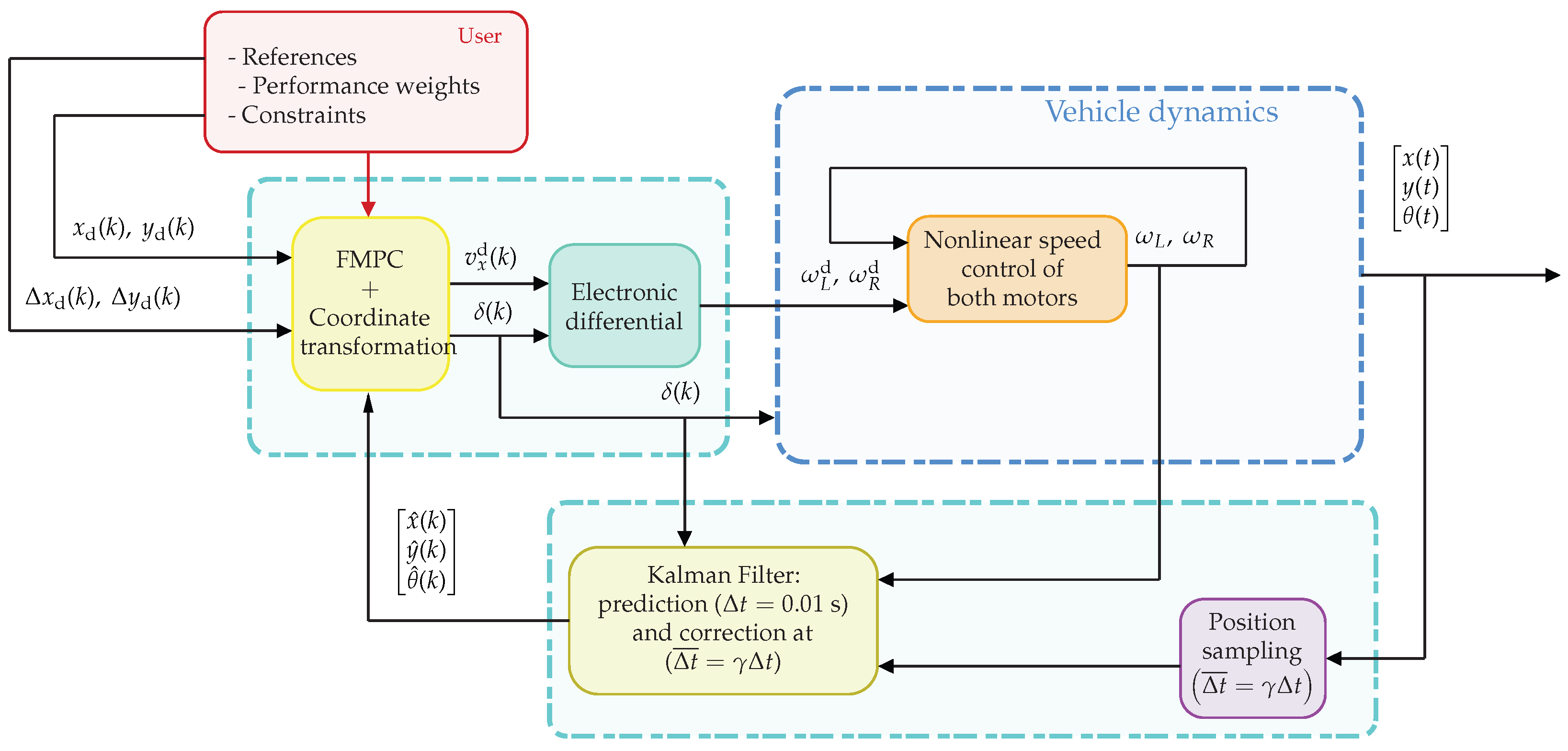
For that, one proposes the strategy depicted in Figure 3. The schema is composed of three main blocks:
- A high-level control block is charged to generate the linear and angular velocity profiles while maintaining the specified constraints on the state and maximum velocities given by the user. The core of this stage is a Frugal Model Predictive Control.
- A low-level dynamic control law is charged to achieve and maintain the desired angular velocity in each motor, which is dictated by the high-level control. This control law must reject the disturbances and uncertainties in the traction system model.
- An Extended Kalman Filter fuses the odometry, sampled at s, and the position measurement obtained by the motion capture system, sampled at , with .
Figure 3.
Proposed control architecture.
3. Control and State Estimation Strategy
In this section, each block of the general schema shown in Figure 3 is described in detail.
3.1. FMPC Applied to the Car-like Mobile Robot
The kinematic model of a car-like mobile robot defined in (1) is a nonlinear system of equations; movement of the body is described by trigonometric functions of the orientation angle . Besides, because the center of mass is set at the rear axle, the vehicle cannot have instantaneous lateral movement (non-holonomic restriction). To avoid this limitation, the reference point is moved p along the vehicle. The objective is to obtain a function that describes the relationship between the new reference point P and the state of the system . The coordinates of P with respect to the inertial frame are given by
the new point depends on the orientation . To determine how that point moves over time, the new position expressions are differentiated. From Figure 4, the displacement of the new point P on the inertial frame is described by
Figure 4.
Reference point displaced p distance from rear wheel for feedback linearization.
Let us define the following coordinate change:
where is a control vector that will later be designed to track the reference position. Note that represents the linear velocity of the point P expressed in the inertial frame. Using (17) in (16), gives
This representation provides a decoupled framework that facilitates the application of linear control techniques while maintaining the essential fidelity of the original kinematic model.
Assumption 2.
The distance p of the virtual point, called “nose,” is constant.
3.1.1. Plant Model for the FMPC
3.1.2. Discretization by Zero-Order Hold
Let be the sampling period. Applying a zero-order hold (ZOH) discretisation scheme to (20) yields the discrete-time model
where the discrete matrices are
3.1.3. Predictive Scheme
Starting from the model (22), the N-step-ahead state prediction is constructed following the procedure in [60,63]. Concatenating predictions for yields the compact form
where and are the stacked state and input sequences over the horizon, and
with being the block-selection matrix that extracts the j-th input from , i.e., .
The regulated and constrained outputs are the Cartesian positions and , selected by means of the following:
The quadratic cost function penalizing position-tracking error and control effort over the horizon N is as was presented in the Equation (10) where . Expanding (10) using (24) and dropping terms that are constant with respect to yields the standard quadratic form [63]:
where
Note that is computed offline once for all, while is updated at every sampling instant k using the current state and the future reference sequence .
The constrained optimal control sequence is the solution of the quadratic programming problem (QOP),
subject to the hard constraints listed in Table 1:
The receding-horizon law applies only the first element of the optimal sequence:
Table 1.
Operational constraints for the car-like mobile robot.
3.1.4. Frugal Control Parametrization
For a prediction horizon N and inputs, the full decision vector would require solving a QOP with variables at every sampling instant. For embedded real-time use, this may exceed the available budget .
To reduce the computational load while preserving tracking performance, a frugal control parametrization is adopted [60,63]. Instead of optimizing independently all components, the input sequence is expressed as a linear function of a compact decision vector through a parametrization matrix :
A two-node piecewise-constant profile is adopted: the first node value is held constant over the first half of the horizon, and the second value over the second half. For N steps split at , the parametrization reads as
so that , i.e., the number of decision variables is reduced from to just 4, independently of the chosen horizon length. The resulting parametrization matrix is
where the upper block-rows correspond to node 1 and the lower block-rows to node 2.
Substituting (37) into (27) and the inequality constraints transforms the original QOP into the reduced problem,
subject to , where the reduced matrices are
and are obtained by mapping the constraints (33)–(35) through [60]. is computed offline; only and need to be updated online. Finally, the receding-horizon control law is recovered as
Remark 1.
Note that the control represents the desired linear velocity at the instant k such that the point P in the mobile frame follows the desired trajectory. Then, must be mapped to the desired angular velocities of each wheel. For that, at the instant k, the vector is computed via in (17), and the steering angle is later derived from (2). Then, using (7) and (8) gives
The complete FMPC structure for the car-like mobile robot is summarized in Figure 3. The user supplies the position constraints, weighting matrices and , and the reference trajectory; the FMPC block computes from the reduced QOP at every sampling instant k and issues the corresponding velocity and steering commands to the vehicle.
3.2. Nonlinear Dynamic Control for the Wheel Speed
The wheels in the mobile robot are actuated by DC-motors. Then, the angular velocity dynamics, in continuous-time, for each wheel is given by
a and b are constants that depend on the electrical and mechanical parameters of the motor and will be assumed to be uncertain in this work. is the applied voltage (control) and represents a signal that concentrates external disturbances, originating from the normal and tangential forces present in the wheels of the vehicle and reflected as a moment of forces around the rotational axis. In the following, the temporary variable t will be omitted unless the context requires it.
To establish a simple but robust dynamic controller, the dynamics (45) can be further written as
where and are assumed unknown. The control objective is to guaranty that , when regardless of uncertainties in the model denoted by , and the disturbance which represents the sum of endogenous and exogenous disturbances and can be a time variant.
Before stating the main result, it is important to establish the following considerations:
- such that ;
- ;
- , ∀;
- .
Definition 1
(Saturation function). Given a positive constant M, the continuous and non decreasing function is defined as
Proposition 1.
Consider the system (46) with the dynamic control law
with . Let us define and as the tracking error and the estimation error, respectively. In addition, consider as the state vector in the error’s coordinates. Then, after a long enough time, the error vector converges to the neighborhood of the origin.
was previously defined and is the highest eigenvalue of the matrix , where is given by
The proof is given in Appendix A.
Remark 2.
Note that this low-level control law, (48), is designed in continuous-time but implemented in discrete-time in an embedded microprocessor running to a frequency higher than the high-level control given by the FMPC.
3.3. Extended Kalman Filter for State Estimation
In navigation applications, whether indoors or outdoors, it is common to utilize multiple sensors (such as encoders, cameras, laser sensors, ultrasonic sensors, IMUs, and GPS) to measure or estimate the vehicle’s position. To reduce trajectory-tracking errors, it is essential for the mobile robot’s current position to be accurate, as this accuracy allows the tracking controller to generate optimal control commands.
The Extended Kalman Filter (EKF) is a version of the Kalman filter designed for nonlinear systems [64]. While the standard filter only works optimally in linear systems, the EKF allows the state of more complex systems to be estimated via linearization. The fusion of sensory data with the Extended Kalman Filter (EKF) is enabled by a two-step iterative process that combines a mathematical model of the system with actual measurements from multiple sensors, assigning a weight to each measurement based on its uncertainty. The algorithm employs the Kalman gain to dynamically balance model prediction and sensor measurement based on their respective uncertainties. The state and uncertainty are projected forward using a nonlinear transition model based on the system’s physical laws. This distinguishes it from the standard Kalman Filter, which relies on a linear state-space representation. The discrete-time kinematic bicycle model (1) based on wheel speeds (4), which defines the state , is given by
where denotes the sampling interval between updates and is the process noise vector, accounting for modeling inaccuracies and external disturbances in the robot’s motion.
Since the EKF operates on a linear approximation of the system dynamics, we linearize at each time step around the current operating point. This allows for the forward propagation of the state uncertainty. The corresponding Jacobian is expressed as
An OptiTrack system provides direct state observations, yielding a linear measurement model. Under the assumption of full state observability, the observation function is defined by
where represents the actual measurements at time k, while accounts for the additive measurement noise. To facilitate filter update, the measurement model is linearized about the current predicted state as follows:
The stochastic components of the model, namely the process noise and measurement noise , are assumed to be zero-mean additive White Gaussian Noise (WGN). These are characterized by their respective covariance matrices and . In this study, the measurement noise covariance is empirically determined on the basis of the static precision of the OptiTrack system:
The covariance matrix represents the uncertainties in the kinematic model, incorporating errors such as wheel slippage and surface irregularities. Following the approach in [65], this is defined based on the expected variability of control inputs and motion model noise. Under the assumption that the noise in the steering angle and wheel speeds are independent and Gaussian, the matrix is expressed as
where , and are the variance of the prediction states (). The EKF algorithm operates iteratively through the following two main phases.
3.3.1. Prediction
In the first stage, the state vector is projected forward using the nonlinear motion model:
The state covariance is propagated through the linearized system dynamics:
3.3.2. Update
The innovation vector represents the discrepancy between the actual sensor measurement and the predicted observation:
Once a measurement is available, the Kalman gain is computed to weigh the reliability of the sensors:
In the final step, the posteriori state estimate and its associated covariance are refined by means of the calculated Kalman gain:
By iteratively applying these prediction and correction phases, the EKF minimizes the estimation error covariance, providing a robust tracking of the vehicle’s trajectory.
4. Experimental Platform Description
To validate the control strategy, an ecosystem was developed for the experimental deployment and analysis of the results. This ecosystem consists of three main components: (1) a real-time localization system (RTLS), (2) a car-like robot equipped with an open-architecture autopilot, and (3) a control station responsible for (i) processing information from the RTLS, (ii) executing the control strategy, and (iii) sending the desired steer angle and the desired angular velocity to each motor of the vehicle so that deployment tasks are executed. Figure 5 shows the described ecosystem.
Figure 5.
The experimental platform is divided into four key workspaces: the Wi-Fi communication network, the ground control station, the motion capture (MoCap) system, and the navigation test area. The main components include a local router, a ground station for executing control algorithms, MoCap equipment, and the mobile robot. To view a video of the experiment, please visit https://www.youtube.com/watch?v=MQM11T2g1CE or scan the QR code. Accessed on 1 May 2026.
The ground station features are a 12th-generation Core i7-1255U 1.7 GHz processor, 12 GB RAM, Ubuntu 22.04 LTS, and MATLAB 2024B. The onboard controller operates under the ESP32 Devkit v1 together with the board based on a STM32H7 microcontroller, allowing operation in a 100 Hz control loop.
4.1. RTLS
The localization stage is based on a motion capture (MoCap) system comprising a network of infrared cameras and specialized software that allows real-time monitoring of an object’s movement from light reflected by markers attached to the vehicle. In this case, the Optitrack system was used, which provides the pose, a 6-DoF tracking vector: 3 DoF for position and 3 DoF for orientation of the vehicle. In our case, only 2 DoF for position and 1 DoF for orientation are used.
4.2. Robotic Platform
The physical agent is a car-like mobile robot, characterized by non-holonomic constraints (Ackermann-steering vehicle). It is equipped with two 12V DC encoder motors on the rear axle and a controller on board for speed control and wireless communication. Table 1 details the platform characteristics.
4.3. Control Station
The control station (CS) acts as the system’s central hub, utilizing ROS2 Humble to manage data distribution. It publishes the vehicle’s pose to a high-level FMPC trajectory-tracking controller within the MATLAB 2024B environment. Furthermore, the CS processes wheel speed data through an Extended Kalman Filter (EKF), fusing it with kinematic odometry to provide a robust pose estimation for the car-like robot. All system variables are monitored in real-time through the control station.
4.4. Extended Kalman Filtering Tuning
For computational efficiency, the process noise covariance matrix, , is assumed to be diagonal, where each element represents the error variance of the corresponding state component (Equation (56)). The terms and are modeled as proportional to the traveled distance and velocity, whereas accounts for uncertainties during rotational maneuvers. Experimental calibration is performed through straight-line motion at a constant velocity to characterize the position error variances and . Analogously, is determined through controlled rotation tests. A high-magnitude de-weights the odometry model in favor of external correction sensors, whereas a low-magnitude prioritizes the dead reckoning estimates.
To ensure the reproducibility of the estimation stage, the EKF parameters are provided. The process noise covariance matrix was set to
The measurement noise covariance matrix was characterized based on the OptiTrack motion capture system’s precision (with an experimental < 2 mm):
Regarding the prediction stage, the geometric parameters required for odometry and state estimation are summarized in Table 2.
Table 2.
Car-like mobile robot platform parameters.
4.5. Experiment Description
To validate the proposed control scheme and evaluate the integrated subsystems, five experiments were designed, each repeated 10 times to assess reliability. In all cases, the objective was to track a time-parameterized lemniscate trajectory. The trajectory is defined by the following parametric equations:
where and represent the amplitude of the trajectory and the angular frequency, respectively.
The proposed trajectory-tracking strategy is based on a kinematic bicycle model, focusing exclusively on planar translation velocities and the yaw rate (). Given that the high-level Model Predictive Control (MPC) employs a kinematic model linearized through input–output feedback linearization (shifted output), dynamic effects such as lateral and rolling forces are inherently excluded from the formulation. Consequently, the operational range is restricted to low-speed maneuvers, where the non-slip assumption remains valid and dynamic perturbations can be effectively mitigated by the low-level controllers, which incorporate disturbance observers for the traction units. Furthermore, the electronic differential algorithm remains applicable under these conditions. To ensure the physical consistency of the zero-slip hypothesis during experimental validation, high-density EVA foam was utilized to provide a high-friction contact surface. The actuator constraints and the steering limits of the car-like mobile robot are summarized in Table 2.
- Experiment 1. The objective of this test is to evaluate the performance of the FMPC relative to a Linear Quadratic Regulator (LQR) using identical cost matrices. Furthermore, trajectory-tracking precision is assessed at a control frequency of 100 Hz, while the EKF-based sensor fusion is validated using a 1 Hz correction rate to test the system’s robustness under low-frequency updates.
- Experiment 2. Leveraging the enhanced capabilities of the EKF-based framework, this test evaluates how state estimation bolsters the robustness of trajectory tracking. The architecture facilitates multi-rate operation, decoupling the high-frequency control execution from the lower-frequency pose measurements. Specifically, the EKF prediction stage and the control loop operate at a 10 ms sampling period, whereas the EKF correction stage is triggered at a 4 s interval to assess the system’s dead-reckoning reliability during sensor latency.
- Experiment 3. A fundamental advantage of Model Predictive Control (MPC) is its inherent capability to incorporate explicit state and control input constraints. This experiment validates this feature by imposing the state constraint , ensuring the car-like robot’s pose remains within a predefined safe operating range. The boundaries for the linear trajectory were set to m, while for the circular path, they were defined as m. To further challenge the controller’s constraint-handling capabilities, the trajectory amplitude was increased to m, exceeding the m used in previous benchmarks.
- Experiment 4. The robustness of the control scheme against external disturbances was evaluated through the low-level controller. This controller features a nonlinear structure integrated with an input-based disturbance observer. To test its ability to regulate wheel speed under variable conditions, an additional payload of 896 g was added to the vehicle. Within the trajectory-tracking framework, the vehicle is required to track a specific velocity profile to ensure spatial accuracy at every time step. Therefore, the low-level control must effectively compensate for the added mass and maintain the velocity within the bounds defined by the high-level trajectory-tracking algorithm.
- A central contribution of this work is the computational efficiency of the control scheme. Specifically, motor control, data fusion for pose estimation, and the trajectory-tracking algorithm are executed within a 10 ms sampling interval, necessitating a low computational overhead. To evaluate the impact of the proposed FMPC parameterization on both execution time and tracking precision, its performance was benchmarked against a conventional, non-parameterized MPC.
5. Experimental Results
5.1. Experiment 1: DLQR vs. FMPC
To validate the proposed control scheme and ensure a fair comparison, a Digital Linear Quadratic Regulator (DLQR) was developed, as both approaches are categorized as optimal control strategies and were tested under identical conditions. The resulting time-series trajectory tracking for each state is presented in Figure 6. The dashed black line represents the reference, while solid lines and shaded areas denote the mean () and confidence intervals () for DLQR (orange) and FMPC (blue), maintaining consistency across all comparative results. It is observed that the FMPC (blue line) exhibits a slightly more pronounced initial transient in the y-axis—an expected behavior due to the imposed constraints—yet it successfully converges to the reference smoothly. Both controllers demonstrate excellent tracking capabilities relative to the reference signals. Furthermore, the uncertainty bands () suggest that the FMPC maintains a competitive variance against the DLQR, which is noteworthy given that the FMPC solves a constrained optimization problem at each time step. The shaded regions in the plot indicate uncertainty peaks during abrupt changes in direction; however, the FMPC effectively manages these high-dynamic regions with a controlled standard deviation.
Figure 6.
DLQR vs. FMPC with correction at 1 s.
The Figure 7 illustrates the control effort for the traction motors () and the steering angle (). The DLQR exhibits higher variance and more aggressive oscillations, which could lead to mechanical fatigue or actuator damage in a physical implementation. Furthermore, the motor velocity profiles for the FMPC are smoother, indicating a more energy-efficient control action compared to the DLQR, while maintaining competitive tracking performance.
Figure 7.
Control signals in DLQR vs. FMPC comparison.
The trajectory-tracking performance in the phase space (x-y plane) is shown in Figure 8. As previously identified in the time-series state dynamics, both approaches achieve successful tracking of the reference trajectory, despite the EKF pose correction occurring at a low frequency of 1 Hz. Notably, the FMPC exhibits more reliable behavior due to its iterative optimization process at each sampling instant; consequently, the steady-state covariance once the trajectory is reached is minimal. Furthermore, its predictive horizon allows the system to anticipate the desired path, resulting in a smoother initial response. In contrast, while the DLQR is also capable of ensuring correct trajectory following, its repeatability is lower. This is attributed to its reactive nature when responding to positioning errors, despite its inherent optimal formulation.
Figure 8.
The trajectory-tracking performance in the phase space (x-y) plane for DLQR vs. FMPC.
To quantitatively evaluate the tracking performance, three integral error criteria were computed: Integral Square Error (ISE), Integral Absolute Error (IAE), and Integral Time-weighted Absolute Error (ITAE). The resulting metrics are presented in Table 3. It is important to note that these metrics were calculated after an initial transient period (t > 5 s) to ensure that the comparison reflects the controllers’ ability to maintain the trajectory rather than their initial convergence speed. As shown in Figure 9, the FMPC consistently outperforms the DLQR across all metrics. The significantly lower ISE and ITAE values demonstrate that the FMPC achieves higher tracking fidelity and superior convergence stability, effectively mitigating cumulative errors that the reactive DLQR fails to suppress over time.
Table 3.
Quantitative evaluation of tracking precision for Experiment 1. The table summarizes ISE, IAE, and ITAE values for both DLQR and FMPC implementations.
Figure 9.
ISE, IAE, and ITAE evolution for both DLQR and FMPC with correction at 1 s.
5.2. Experiment 2: Validation of Pose Estimation Under Multi-Rate EKF Correction Frequencies
The complete control architecture is where all the processes are synchronized at a high-frequency sampling rate of 100 Hz (10 ms). This rapid execution cycle ensures seamless interaction between the EKF-based state estimation and the FMPC law. As evidenced by the time-series plots in Figure 10, the Extended Kalman Filter provides a robust, low-latency pose estimate, effectively mitigating sensor noise while maintaining high-fidelity tracking of the vehicle’s rapid dynamics. The actuator responses for the traction motors () and the steering angle () demonstrate near-perfect alignment with the required setpoints, even during aggressive maneuvers (as shown in Figure 11).
Figure 10.
States evolution along the time of FMPC with EKF correction at 10 ms.
Figure 11.
Control signals for FMPC with EKF correction at 10 ms.
Phase-space analysis confirms exceptional trajectory repeatability, characterized by minimal steady-state variance captured in Figure 12. These results definitively validate the real-time feasibility and computational efficiency of the proposed hierarchical scheme on an embedded platform.
Figure 12.
Trajectory-tracking performance of control schema with EKF correction at 10 ms.
To evaluate the system’s reliability during sensor degradation or low-frequency positioning updates, the EKF correction stage was throttled to a 4-s interval. As illustrated in Figure 13, Figure 14 and Figure 15, the hierarchical scheme maintains trajectory integrity through extended periods of dead-reckoning. The time-series analysis reveals that the EKF prediction stage successfully bridges the 4-s gaps between measurements, preventing the controller from becoming unstable. Although the phase-space plots show a marginal increase in the confidence intervals ()—typical of cumulative odometric drift—the FMPC effectively manages this uncertainty, resulting in a smooth path that converges back to the reference upon each sensor update. These results confirm the high robustness of the proposed estimator–controller pair under extreme feedback latency. Furthermore, this experiment effectively simulates a GPS-denied environment or a scenario with significant sensor occlusion, where the vehicle must rely solely on its internal kinematic model and odometry for extended periods. Despite the 4-s latency, the FMPC demonstrates remarkable smoothness during the state-correction instances. Rather than exhibiting abrupt ’jumps’ or erratic steering behavior when a new measurement is received, the controller leverages its optimization-based nature to seamlessly re-integrate the updated pose into the predictive plan. This ability to maintain dynamic stability under extreme feedback sparsity highlights the reliability of the proposed hierarchical framework for real-world autonomous missions where sensor reliability cannot be guaranteed.
Figure 13.
x, y and states evolution at 4 s correction rate.
Figure 14.
Car-like mobile robot control signals (wheels’ speeds and steering angle) at 4 s rate correction.
Figure 15.
Trajectory-tracking performance of mobile robot at 4 s rate correction.
The comparative performance analysis under variable correction rates is presented in Figure 16 and Table 4, the cumulative error metrics (ISE, IAE, and ITAE) for three distinct EKF correction intervals are 10 ms, 1 s, and 4 s.
Figure 16.
Performance for EKF each correction time.
Table 4.
Performance metrics (ISE, IAE, and ITAE) of the FMPC-EKF scheme across different pose correction sampling periods.
A key finding is the minimal performance gap between the 10 ms and 1 s correction rates, indicating that the EKF effectively bridges the feedback latency without significant degradation in tracking precision. While the 4 s correction interval (green line) exhibits higher cumulative error—attributable to the prolonged periods of open-loop odometric prediction—it maintains a stable and predictable trend. The fact that the ITAE slope remains bounded even under such sparse feedback conditions validates the robustness of the FMPC-EKF pair, confirming its suitability for autonomous navigation in environments with intermittent sensor availability.
5.3. Experiment 3: State Constraint Handling
Regarding the operational constraints, Figure 17 demonstrates the FMPC’s ability to enforce strict operational boundaries, specifically the lateral state constraint . In both the linear (a) and circular (b) tracking scenarios, the FMPC successfully confines the robot’s pose within the predefined safe zones (indicated by the red-shaded regions). As observed in the plots, whenever the reference trajectory exceeds the safety limits, the controller prioritizes constraint satisfaction over reference tracking, effectively saturating the state at the boundary. The phase-space plots further confirm this behavior, showing how the vehicle’s trajectory is ‘compressed’ to stay within the allowable x-range. This inherent safety feature is critical for autonomous navigation in constrained environments, proving that the proposed hierarchical scheme ensures collision avoidance and regulatory compliance through its active optimization-based framework.
Figure 17.
Constrained scenarios. (a) Straight line as a reference, and (b) circle as a reference.
5.4. Experiment 4: Load Disturbance Compensation
In trajectory tracking, precise longitudinal speed control is critical due to the time-dependent nature of the reference trajectory. As illustrated in the upper plots of Figure 18, the wheel angular velocities successfully track the reference signals generated by the electronic differential, even under an 896 g payload. Despite the dynamic effects introduced by the additional mass, the tracking error remains within acceptable margins. This performance is attributed to the low-level controller, which incorporates a control-input-based disturbance observer and explicitly accounts for actuator saturation limits. The lower plots of Figure 18 depict the evolution of the disturbance estimation for both the left and right wheel motors. The observer effectively compensates for the added mass, which is reflected in the increased magnitude of the control signals. Notably, this increase is more pronounced in the left motor; although the payload was intended to be centered, its final placement fell slightly toward the left side. The control scheme successfully identified and compensated for this experimental asymmetry, maintaining system stability. The narrow variance () shown in the shaded regions of Figure 19 indicates high repeatability. Furthermore, while the performance indices (Figure 20) show a cumulative increase in tracking error—particularly the ITAE, which rises more sharply during segments of maximum curvature, the state-phase diagram confirms that this deviation is not significant. Ultimately, the vehicle maintains high fidelity to the lemniscate geometry, demonstrating that the proposed control scheme is robust against both significant payloads and unmodeled mass distributions. Table 5 summarizes ISE, IAE, and ITAE values for both nominal and loaded conditions.
Figure 18.
Comparison of low-level control signals under nominal and loaded conditions.
Figure 19.
Comparison of trajectory-tracking performance: nominal vs. loaded conditions.
Figure 20.
Tracking error metrics comparison for nominal and loaded experimental scenarios.
Table 5.
Quantitative evaluation of tracking error for Experiment 4 (Load Disturbance Compensation).
5.5. Experiment 5: MPC vs. FMPC (Computational Cost)
The practical feasibility of the proposed hierarchical control scheme is central to its application in real-world environments. The architecture aims to achieve precise and robust trajectory tracking under strict constraints within a 10 ms sampling interval. This enables the potential deployment of the algorithm on embedded platforms with limited computational resources. To validate the optimization of the computational load, the proposed FMPC was benchmarked against a conventional, non-parameterized MPC. Both controllers utilized the same double-integrator model, identical constraints, cost-function weighting matrices, and numerical solver. As shown in Figure 21 and Table 6, the FMPC significantly reduces computational overhead while simultaneously improving tracking precision, yielding lower error values across all performance indices (ISE, IAE, and ITAE). Regarding execution time (Figure 22), the conventional MPC operates near the sampling limit, with its variance () frequently exceeding the 10 ms threshold. Conversely, the FMPC consistently solves the optimization problem well below the sampling period with negligible variance.
Figure 21.
First figure of the calculation time comparison.
Table 6.
MPC vs. FMPC metrics.
Figure 22.
Second figure of the calculation time comparison.
These results highlight the superior real-time performance of the FMPC and its suitability for fully embedded implementation.
6. Empirical Stability Analysis via Cost-Function Evolution
To provide empirical evidence of the closed-loop stability properties of the proposed FMPC algorithm, the temporal evolution of the cost function and its first-order increment were evaluated along ten independent experimental runs as described in experiments 1, 2, and 4. At each sampling instant, was computed according to the standard quadratic form (10) with , ms, and the steady-state input obtained from the standard rank condition associated with the augmented system matrix, in agreement with the classical reference-tracking formulation. The evaluation was performed on measured states and applied control inputs, so that the resulting trajectory of reflects the actual closed-loop behavior of the plant rather than the predicted optimum of the underlying quadratic program.
The upper subplot of the Figure 23 reveals three distinct phases. During the initial transient ( s), the cost decreases by nearly two orders of magnitude, dropping from to a residual value below 150. The subsequent regime exhibits a bounded steady-state behavior in which remains confined within a small neighborhood of zero, punctuated by mild periodic excursions of approximately 250 units occurring at , 10, and 15 s. These excursions are consistent with the geometry of the reference: the lemniscate exhibits regions of maximal curvature at its central crossing and outer apices, where the tracking task becomes most demanding due to abrupt changes in the desired velocity vector. The periodicity, magnitude, and phase of these features are reproducible across the ten experimental runs, as evidenced by the narrow confidence bands surrounding the mean trajectory.
Figure 23.
Cost function evolution.
The increment , displayed in the lower subplot, provides the more discriminating diagnostic. A short-lived positive lobe is observed during the first ∼0.4 s of operation, attributable to the physical inertia of the actuators; as the reference begins to evolve from rest, the cart cannot instantaneously match the prescribed velocity profile, causing the tracking error to grow over a small number of samples before the controller asserts effective authority. This phenomenon is intrinsic to any sampled-data implementation operating on real hardware and does not constitute a violation of the Lyapunov-type descent property of MPC, which is rigorously established for the value function associated with the optimal control sequence rather than for the realized cost computed from measured signals. Once the actuators reach an operating regime compatible with the reference dynamics, becomes strongly negative, attaining values of approximately during the dominant decay phase. After convergence to the steady-state regime, oscillates in a tight neighborhood of zero, with both positive and negative excursions remaining below 5% of the peak descent rate observed during the transient.
The aggregate behavior is fully consistent with the Lyapunov-based stability arguments that are standard in the predictive control literature. The cost function exhibits an overall monotonic decrease over the transient phase, ultimate boundedness in the steady-state phase, and a contraction ratio of that quantifies the controller’s regulating action. The minor positive excursions of in the steady-state regime are explained by two well-understood mechanisms: first, the reference is not an equilibrium of the system but a periodic, non-stationary trajectory, so the cost cannot decay to zero but only to a residual level dictated by the curvature-induced infeasibility of perfect tracking; second, the cost is evaluated on the realized closed-loop trajectory rather than on the optimal predicted one, introducing a non-negative gap whose fluctuation is consistent with observed measurement noise and unmodeled dynamics. Critically, the standard deviation across the ten runs remains an order of magnitude smaller than the mean throughout the entire experiment, confirming that the observed convergence behavior is a structural property of the closed loop rather than a fortunate artifact of any particular trial. Taken together, these observations constitute strong empirical evidence that the proposed FMPC algorithm enforces practical asymptotic stability of the tracking error and exhibits the descent behavior expected of a properly tuned predictive control law.
7. Conclusions
This work presents a hierarchical control architecture for high-precision trajectory tracking of a car-like mobile robot operating under significant disturbances originating from the normal and tangential forces present in the wheels of the vehicle. The proposed framework integrates a low-level nonlinear dynamic controller with a high-level frugal model predictive controller, enabling simultaneous disturbance rejection and accurate path tracking at a prescribed cruise velocity. Experimental results demonstrate that the integration of disturbance-compensating low-level control, predictive high-level planning, and sensor-fusion-based state estimation provides an effective solution for reliable autonomous navigation in challenging environments. Future work will focus on extending the framework to fully onboard sensing systems, adapting the predictive layer to accommodate varying terrain conditions, and exploring cooperative implementations in multi-vehicle robotic systems.
A significant limitation of the current control scheme is its reliance on a kinematic bicycle model, which fails to guarantee stability or feasibility in high-speed maneuvers. To address this, future research will incorporate the bicycle’s dynamic model into the MPC framework. This will allow the system to compensate for lateral forces and varying tire-road friction, ensuring stability at higher velocities. Additionally, we aim to investigate a path-following reformulation where the trajectory is parameterized in the spatial domain. By representing the prediction model as a chain of integrators or decoupled double integrators, the MPC can be solved as a quadratic programming (QP) problem, significantly enhancing real-time computational efficiency.
Author Contributions
Conceptualization, L.A.M.-R., R.I.V.-C. and J.F.G.-C.; methodology, J.F.G.-C. and W.F.G.-S.; software, L.A.M.-R.; validation, L.A.M.-R. and R.I.V.-C.; formal analysis, J.F.G.-C.; investigation, G.A.M.-H.; resources, G.M.-A.; data curation, R.I.V.-C.; writing—original draft preparation, L.A.M.-R. and R.I.V.-C.; writing—review and editing, J.F.G.-C. and R.C.A.-L.; visualization, R.I.V.-C.; supervision, R.C.A.-L. and G.M.-A.; project administration, W.F.G.-S.; funding acquisition, G.A.M.-H., G.M.-A. and J.F.G.-C. All authors have read and agreed to the published version of the manuscript.
Funding
This research was partially funded by Vicerrectoría de Investigación y Estudios de Posgrado de la BUAP (VIEP-BUAP) grant number 00593-PV/2025.
Data Availability Statement
The original contributions presented in this study are included in the article. Further inquiries can be directed to the corresponding author.
Acknowledgments
The first and second authors acknowledge support from the Secretariat of Science, Humanities, Technology, and Innovation (SECIHTI) in Mexico, for supporting their Ph.D. studies at BUAP through a scholarship.
Conflicts of Interest
The authors declare no conflicts of interest.
Appendix A
Proof of Proposition 1
Proof.
First, note that the variable given in the first equation of (48) has bounded trajectories:
Now, consider the dynamics of the error variables:
Since is bounded, it is assured that remains bounded. Now, the trajectories of will be analyzed. For this, the following candidate Lyapunov function is proposed:
We derive along the system trajectory,
Assuming that then with small enough. Due to the boundedness of we can discern that
and for this reason . This means that has the same sign as , i.e., the same sign as . Now, considering that it must be true that
Assume that:
It can be ensured that the function decreases, i.e., ; consequently, the variable enters the set:
Upon entering this set, evolves in the linear part of , therefore the system (A2) becomes
Rewriting the system in matrix form, we have
To determine the stability of (A10), the eigenvalues of must be analyzed:
Thus, the characteristic polynomial is defined as
Since , then is a Hurwitz matrix. Thus, for the system given by
the trajectories of the error vector can be bounded by
where is the highest eigenvalue □
References
- Chen, Z.; Yin, J.; Farhan, S.M.; Liu, L.; Zhang, D.; Zhou, M.; Cheng, J. A comprehensive review of obstacle avoidance for autonomous agricultural machinery in multi-operational environment. Artif. Intell. Agric. 2026, 16, 139–163. [Google Scholar] [CrossRef] [Scilit]
- Yang, J.; Zulkarnain, N.; Faisal Ibrahim, M.; Najaa Aimi Mohd Nordin, I.; Abdollah Vaghefi, S. A Comprehensive Review of Agricultural Ground Automatic Navigation Systems Based on Multi-Sensor Fusion. IEEE Access 2025, 13, 168159–168182. [Google Scholar] [CrossRef] [Scilit]
- Khodarahmi, M.; Maihami, V. A Review on Kalman Filter Models. Arch. Comput. Methods Eng. 2023, 30, 727–747. [Google Scholar] [CrossRef] [Scilit]
- Alatise, M.B.; Hancke, G.P. A Review on Challenges of Autonomous Mobile Robot and Sensor Fusion Methods. IEEE Access 2020, 8, 39830–39846. [Google Scholar] [CrossRef] [Scilit]
- Shit, R.C. Precise localization for achieving next-generation autonomous navigation: State-of-the-art, taxonomy and future prospects. Comput. Commun. 2020, 160, 351–374. [Google Scholar] [CrossRef] [Scilit]
- Wang, S.; Ahmad, N.S. A Comprehensive Review on Sensor Fusion Techniques for Localization of a Dynamic Target in GPS-Denied Environments. IEEE Access 2025, 13, 2252–2285. [Google Scholar] [CrossRef] [Scilit]
- Ahmed Amin, A.; Mubarak, A.; Manzoor, H.U. Design of intelligent vehicular and sensor communication network: A comprehensive survey. Syst. Sci. Control Eng. 2025, 13, 2529187. [Google Scholar] [CrossRef] [Scilit]
- Souza De Oliveira, C.; Toledo, R.D.S.; Tulux Oliveira Victorio, V.H.; Von Wangenheim, A. Trajectory Planning for Autonomous Cars in Low-Structured and Unstructured Environments: A Systematic Review. IEEE Access 2025, 13, 48841–48871. [Google Scholar] [CrossRef] [Scilit]
- Erfianti, R.; Asfihani, T.; Suhandri, H.F. GNSS/IMU Sensor Fusion Performance Comparison of a Car Localization in Urban Environment Using Extended Kalman Filter. IOP Conf. Ser. Earth Environ. Sci. 2023, 1127, 012006. [Google Scholar] [CrossRef] [Scilit]
- Teng, X.; Shen, Z.; Huang, L.; Li, H.; Li, W. Multi-sensor fusion based wheeled robot research on indoor positioning method. Results Eng. 2024, 22, 102268. [Google Scholar] [CrossRef] [Scilit]
- Siegwart, R. Introduction to Autonomous Mobile Robots; Intelligent Robots and Autonomous Agents; MIT Press: Cambridge, MA, USA, 2004. [Google Scholar]
- Lynch, K.M.; Park, F.C. Modern Robotics: Mechanics, Planning, and Control, 1st ed.; Cambridge University Press: Cambridge, UK, 2017. [Google Scholar] [CrossRef] [Scilit]
- Kalman, R.E. A New Approach to Linear Filtering and Prediction Problems. J. Basic Eng. 1960, 82, 35–45. [Google Scholar] [CrossRef] [Scilit]
- Crassidis, J.L.; Junkins, J.L. Optimal Estimation of Dynamic Systems; Number 2 in Chapman & Hall CRC Applied Mathematics and Nonlinear Science Series; Chapman & Hall/CRC: Boca Raton, FL, USA, 2004. [Google Scholar]
- Zeng, L.; Guo, S.; Zhu, M.; Duan, H.; Bai, J. An Improved Trilateral Localization Technique Fusing Extended Kalman Filter for Mobile Construction Robot. Buildings 2024, 14, 1026. [Google Scholar] [CrossRef] [Scilit]
- Babri, U.M.; Irfan Haider Jillani, M.; Ahmad, R.; Alam, M.M. Tight Coupling of GNSS and IMU using Extended Kalman Filtering. In Proceedings of the 2024 19th Biennial Baltic Electronics Conference (BEC), Tallinn, Estonia, 2–4 October 2024; pp. 1–6. [Google Scholar] [CrossRef] [Scilit]
- Huang, Z.; Ye, G.; Yang, P.; Yu, W. Application of multi-sensor fusion localization algorithm based on recurrent neural networks. Sci. Rep. 2025, 15, 8195. [Google Scholar] [CrossRef] [Scilit]
- Wang, Y. Comparison of the effectiveness of Extended Kalman Filter and machine learning algorithms in sensor fusion. In Proceedings of the 4th International Conference on Computer, Internet of Things and Control Engineering, Wuhan, China, 1–3 November 2024; pp. 18–24. [Google Scholar] [CrossRef] [Scilit]
- Kumar Reddy Damagatla, R.; Atia, M. Improving EKF-Based IMU/GNSS Fusion Using Machine Learning for IMU Denoising. IEEE Access 2024, 12, 114358–114369. [Google Scholar] [CrossRef] [Scilit]
- Yan, K.; Ma, B. Global Posture Stabilization for the Kinematic Model of a Rear-Axle Driven Car-Like Mobile Robot Considering Obstacle Avoidance. IEEE Robot. Autom. Lett. 2023, 8, 5568–5575. [Google Scholar] [CrossRef] [Scilit]
- Yao, Q.; Tian, Y.; Wang, Q.; Wang, S. Control Strategies on Path Tracking for Autonomous Vehicle: State of the Art and Future Challenges. IEEE Access 2020, 8, 161211–161222. [Google Scholar] [CrossRef] [Scilit]
- Siradjuddin, I.; Prayoga, D.A.; Wibowo, S.; Syaifudin, Y.W.; Wicaksono, R.P.; Achmadiah, M.N. A PID Control Algorithm for Path Tracking of a Nonholonomic Car-Like Robot. In Proceedings of the 2024 IEEE International Symposium on Consumer Technology (ISCT), Kuta, Indonesia, 13–16 August 2024; pp. 305–310. [Google Scholar] [CrossRef] [Scilit]
- Trinh, K.L.T.; Nguyen, H.T. Path tracking control for car-like robots by pid controller with time-varying parameters. Sci. Technol. Dev. J. Eng. Technol. 2022, 5, 1642–1650. [Google Scholar] [CrossRef] [Scilit]
- Yang, T.; Bai, Z.; Li, Z.; Feng, N.; Chen, L. Intelligent Vehicle Lateral Control Method Based on Feedforward + Predictive LQR Algorithm. Actuators 2021, 10, 228. [Google Scholar] [CrossRef] [Scilit]
- Mireles-Perez, C.; Cruz-Ortiz, D.; Salgado, I.; Chairez, I. Backstepping second order sliding mode control for a car-like robot. In Proceedings of the 2022 8th International Conference on Control, Decision and Information Technologies (CoDIT), Istanbul, Turkey, 17–20 May 2022; pp. 463–467. [Google Scholar] [CrossRef] [Scilit]
- Zhang, D.; Huang, Q.; Lu, Q.; Zhang, H. Prescribed-Time Extended State Observer-Based Model Predictive Control for Wheeled Mobile Robots. IEEE Trans. Ind. Electron. 2026, 73, 3187–3198. [Google Scholar] [CrossRef] [Scilit]
- Wang, Z.; Gong, B. ESO-LQR-Based Path Tracking Control for Car-Like Robots. In Proceedings of the 2025 44th Chinese Control Conference (CCC), Chongqing, China, 28–30 July 2025; pp. 3465–3470. [Google Scholar] [CrossRef] [Scilit]
- Zhu, C.; Li, B.; Zhao, C.; Wang, Y. Trajectory Tracking Control of Car-like Mobile Robots Based on Extended State Observer and Backstepping Control. Electronics 2024, 13, 1563. [Google Scholar] [CrossRef] [Scilit]
- Miranda-Colorado, R. Observer-based finite-time control for trajectory tracking of wheeled mobile robots with kinematic disturbances. ISA Trans. 2024, 148, 64–77. [Google Scholar] [CrossRef] [Scilit]
- Miranda-Colorado, R. Sliding-mode control of perturbed wheeled mobile robots with matched disturbances compensation. Int. J. Dyn. Control 2025, 13, 289. [Google Scholar] [CrossRef] [Scilit]
- Al Mahmud, S.; Kamarulariffin, A.; Ibrahim, A.M.; Mohideen, A.J.H. Advancements and Challenges in Mobile Robot Navigation: A Comprehensive Review of Algorithms and Potential for Self-Learning Approaches. J. Intell. Robot. Syst. 2024, 110, 120. [Google Scholar] [CrossRef] [Scilit]
- Shirzadeh, M.; Shojaeefard, M.H.; Amirkhani, A.; Behroozi, H. Adaptive fuzzy nonlinear sliding-mode controller for a car-like robot. In Proceedings of the 2019 5th Conference on Knowledge Based Engineering and Innovation (KBEI), Tehran, Iran, 28 February–1 March 2019; pp. 686–691. [Google Scholar] [CrossRef] [Scilit]
- Camacho, E.F.; Bordons, C. Model Predictive Control; Advanced Textbooks in Control and Signal Processing; Springer: London, UK, 2007. [Google Scholar] [CrossRef] [Scilit]
- Zhu, Z.; Yao, Q.; Shi, Y. Intelligent Vehicle Adaptive Robust Path Tracking Control Strategy Based on MPC and ADRC. Int. J. Automot. Technol. 2026, 27, 651–670. [Google Scholar] [CrossRef] [Scilit]
- Kordi, F.; Mobayen, S.; Rezaalikhani, H.; Nikoukar, J. Hybrid trajectory tracking control of wheeled mobile robots using predictive kinematic control and dynamic robust control. Asian J. Control 2025, 27, 1203–1223. [Google Scholar] [CrossRef] [Scilit]
- Yeom, K. Design of Deep Neural Network Based Model Predictive Controller for a Car-like Mobile Robot. Int. J. Mech. Eng. Robot. Res. 2022, 11, 606–613. [Google Scholar] [CrossRef] [Scilit]
- Bai, G.; Meng, Y.; Liu, L.; Luo, W.; Gu, Q.; Liu, L. Review and Comparison of Path Tracking Based on Model Predictive Control. Electronics 2019, 8, 1077. [Google Scholar] [CrossRef] [Scilit]
- Rosas-Vilchis, A.; De Loza, A.F.; Aguilar, L.T.; Cieslak, J.; Henry, D.; Montiel-Ross, O. Trajectory tracking control for an AutoNOMO vehicle using a decoupling approach. In Proceedings of the 2020 28th Mediterranean Conference on Control and Automation (MED), Saint-Raphaël, France, 15–18 September 2020; pp. 375–380. [Google Scholar] [CrossRef] [Scilit]
- Bascetta, L.; Farina, M.; Gabrielli, A.; Matteucci, M. A feedback linearisation algorithm for single-track models with structural stability properties. Control Eng. Pract. 2022, 128, 105318. [Google Scholar] [CrossRef] [Scilit]
- Tiriolo, C.; Lucia, W. A Set-Theoretic Control Approach to the Trajectory Tracking Problem for Input–Output Linearized Wheeled Mobile Robots. IEEE Control Syst. Lett. 2023, 7, 2347–2352. [Google Scholar] [CrossRef] [Scilit]
- Mohan Rayguru, M.; Rajesh Elara, M.; Ramalingam, B.; Muthugala, M.A.V.J.; Samarakoon, S.M.B.P. A Path Tracking Strategy for Car Like Robots with Sensor Unpredictability and Measurement Errors. Sensors 2020, 20, 3077. [Google Scholar] [CrossRef] [Scilit]
- Yan, K.; Ma, B. A unified controller of global trajectory tracking and posture regulation for a car-like mobile robot. Int. J. Robust Nonlinear Control 2024, 34, 8590–8604. [Google Scholar] [CrossRef] [Scilit]
- De Luca, A.; Oriolo, G.; Samson, C. Feedback control of a nonholonomic car-like robot. In Robot Motion Planning and Control; Thoma, M., Laumond, J.P., Eds.; Springer: Berlin/Heidelberg, Germany, 1998; Volume 229, pp. 171–253. [Google Scholar] [CrossRef] [Scilit]
- Siciliano, B.; Sciavicco, L.; Villani, L.; Oriolo, G. Robotics; Advanced Textbooks in Control and Signal Processing; Springer: London, UK, 2009. [Google Scholar] [CrossRef] [Scilit]
- Pereira, B.S.; Santos, T.L.; Conceicao, A.G. A robust feedback-linearization MPC with artificial target for UGVs. Mechatronics 2025, 110, 103358. [Google Scholar] [CrossRef] [Scilit]
- Yildirim, M.; Oksuztepe, E.; Kurum, H. Design of Electronic Differential System for an Electric Vehicle with Four Independently Controlled In-Wheel PMSM. Adv. Electr. Comput. Eng. 2024, 24, 23–32. [Google Scholar] [CrossRef] [Scilit]
- Julio-Rodríguez, J.D.C.; Santana-Díaz., A.; Ramirez-Mendoza, R.A. Individual Drive-Wheel Energy Management for Rear-Traction Electric Vehicles with In-Wheel Motors. Appl. Sci. 2021, 11, 4679. [Google Scholar] [CrossRef] [Scilit]
- Reséndiz Barrón, A.J.; Flores, Y.J.; García-Rodríguez, F.J.; Medina, A.; Serrano Huerta, D.A. Instrumentation of an Electronic–Mechanical Differential for Electric Vehicles with Hub Motors. World Electr. Veh. J. 2025, 16, 179. [Google Scholar] [CrossRef] [Scilit]
- Sun, H.; Wang, H. Research on Electric Vehicle Differential System Based on Vehicle State Parameter Estimation. Vehicles 2025, 7, 80. [Google Scholar] [CrossRef] [Scilit]
- Daya, J.L.F.; Sanjeevikumar, P.; Blaabjerg, F.; Wheeler, P.W.; Ojo, J.O. Implementation of Wavelet-Based Robust Differential Control for Electric Vehicle Application. IEEE Trans. Power Electron. 2015, 30, 6510–6513. [Google Scholar] [CrossRef] [Scilit]
- Wang, D.; Gao, Y.; Wei, W.; Yu, Q.; Wei, Y.; Li, W.; Fan, Z. Sliding mode observer-based model predictive tracking control for Mecanum-wheeled mobile robot. ISA Trans. 2024, 151, 51–61. [Google Scholar] [CrossRef] [Scilit]
- Abadi, A.; Ayeb, A.; Labbadi, M.; Fofi, D.; Bakir, T.; Mekki, H. Robust Tracking Control of Wheeled Mobile Robot Based on Differential Flatness and Sliding Active Disturbance Rejection Control: Simulations and Experiments. Sensors 2024, 24, 2849. [Google Scholar] [CrossRef] [Scilit]
- Peng, J.; Xiao, H.; Lai, G. Nonlinear Disturbance Observer Incorporated Model Predictive Strategy for Wheeled Mobile Robot’s Trajectory Tracking Control. Int. J. Control Autom. Syst. 2024, 22, 2251–2262. [Google Scholar] [CrossRef] [Scilit]
- Abbasi, S.J.; Lee, S. Enhanced Trajectory Tracking via Disturbance-Observer-Based Modified Sliding Mode Control. Appl. Sci. 2023, 13, 8027. [Google Scholar] [CrossRef] [Scilit]
- Sariyildiz, E. Analysis and Synthesis of Disturbance Observer-Based Digital Robust Motion Control Systems in State Space. IEEE Trans. Ind. Electron. 2025, 72, 8376–8385. [Google Scholar] [CrossRef] [Scilit]
- Balbuena, J.; Sinche, J.; Quiroz, D.; Arce, D.; Villota, E. PlatROB: An open-source, modular, and low-cost hardware platform for mobile robotics and AI education. HardwareX 2026, 25, e00747. [Google Scholar] [CrossRef] [Scilit]
- Li, X.; Patel, S.; Stronzek-Pfeifer, D.; Büskens, C. Indoor Localization for an Autonomous Model Car: A Marker-Based Multi-Sensor Fusion Framework. In Proceedings of the 2023 IEEE 19th International Conference on Automation Science and Engineering (CASE), Auckland, New Zealand, 26–30 August 2023; pp. 1–8. [Google Scholar] [CrossRef] [Scilit]
- Biondo, L.; Vella, A.D.; Vigliani, A. Development, Implementation and Experimental Assessment of Path-Following Controllers on a 1:5 Scale Vehicle Testbed. Machines 2025, 13, 1116. [Google Scholar] [CrossRef] [Scilit]
- Magallan, G.; De Angelo, C.; Bisheimer, G.; Garcia, G. A neighborhood electric vehicle with electronic differential traction control. In Proceedings of the 2008 34th Annual Conference of IEEE Industrial Electronics, Orlando, FL, USA, 10–13 November 2008; pp. 2757–2763. [Google Scholar] [CrossRef] [Scilit]
- Vásquez-Cruz, R.I.; Castellanos-Velasco, E.; Guerrero-Castellanos, J.F. Frugal model predictive control and active disturbance rejection for laser beam steering systems. Control Theory Technol. 2025, 23, 513–528. [Google Scholar] [CrossRef] [Scilit]
- Vásquez-Cruz, R.; Castellanos-Velasco, E.; González-Díaz, V.; Castañeda-Camacho, J.; Guerrero-Castellanos, J. Frugal MPC for quadrotor trajectory control. Mem. Congr. Nac. Control Autom. 2025, 8, 439–444. [Google Scholar] [CrossRef] [Scilit]
- Martínez-Ramírez, L.; Guerrero-Castellanos, J.; Ambrosio-Lázaro, R.; Mino-Aguilar, G.; Sánchez-Santana, J.; Munoz-Hernandez, G. Trajectory tracking control with data fusion and geometric algorithm. Mem. Congr. Nac. Control Autom. 2025, 8, 433–438. [Google Scholar] [CrossRef] [Scilit]
- Alamir, M. Stabilization of Nonlinear Systems Using Receding-Horizon Control Schemes; Lecture Notes in Control and Information Sciences; Springer: London, UK, 2006; Volume 339. [Google Scholar] [CrossRef]
- Brown, R.G.; Hwang, P.Y.C. Introduction to Random Signals and Applied Kalman Filtering: With MATLAB Exercises, 4th ed.; John Wiley & Sons: Hoboken, NJ, USA, 2012. [Google Scholar]
- Nugraha, M.H.; Abdul, F.; Bramantyo, L.; Rijanto, E.; Saputra, R.P.; Mahendra, O. Mobile Robot Localization via Indoor Positioning System and Odometry Fusion. In Proceedings of the 2024 IEEE International Conference on Smart Mechatronics (ICSMech), Yogyakarta, Indonesia, 19–21 November 2024; pp. 1–6. [Google Scholar] [CrossRef] [Scilit]
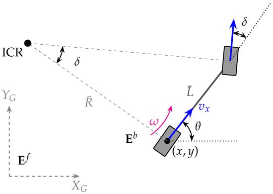
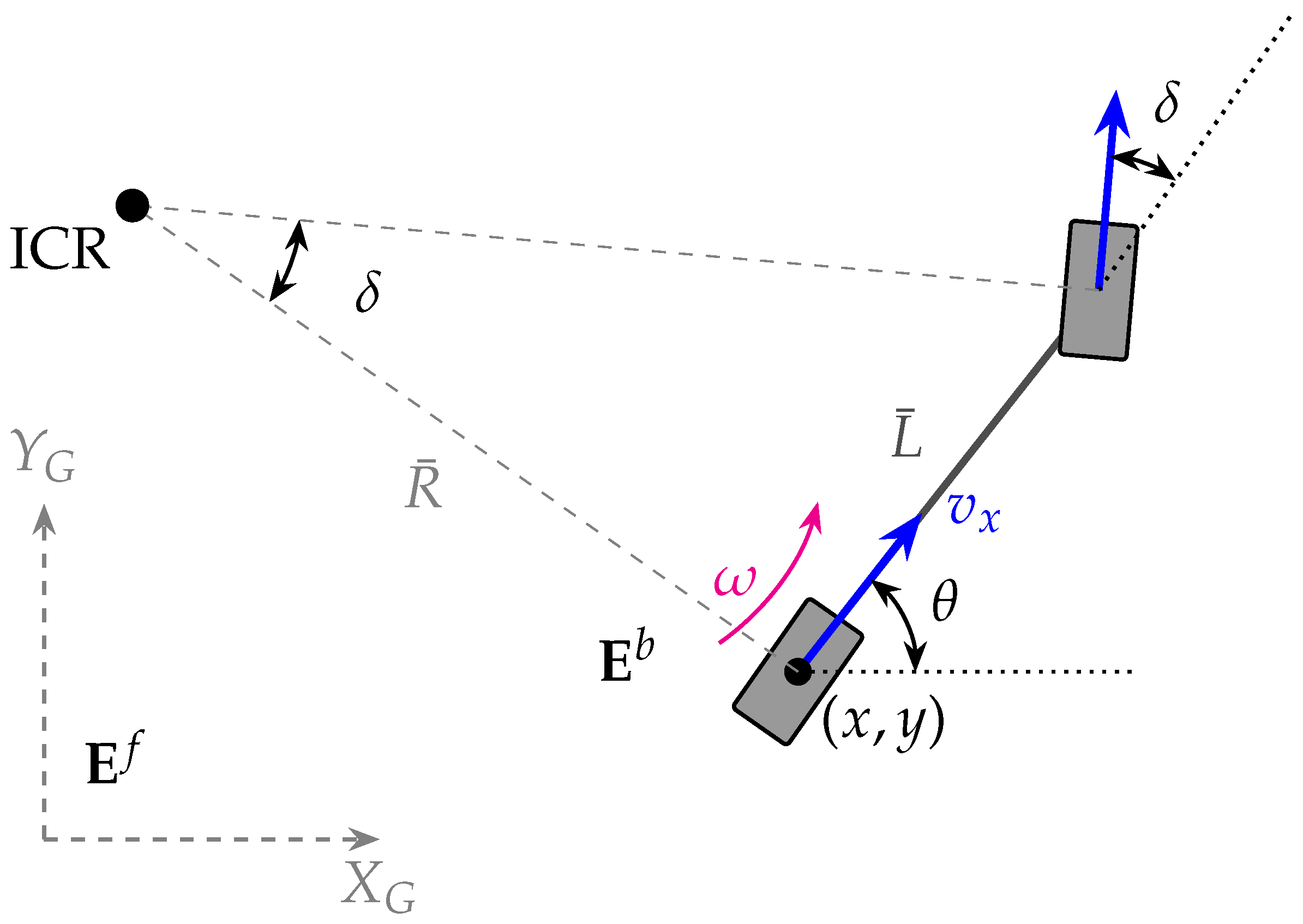
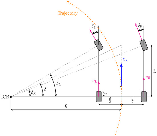
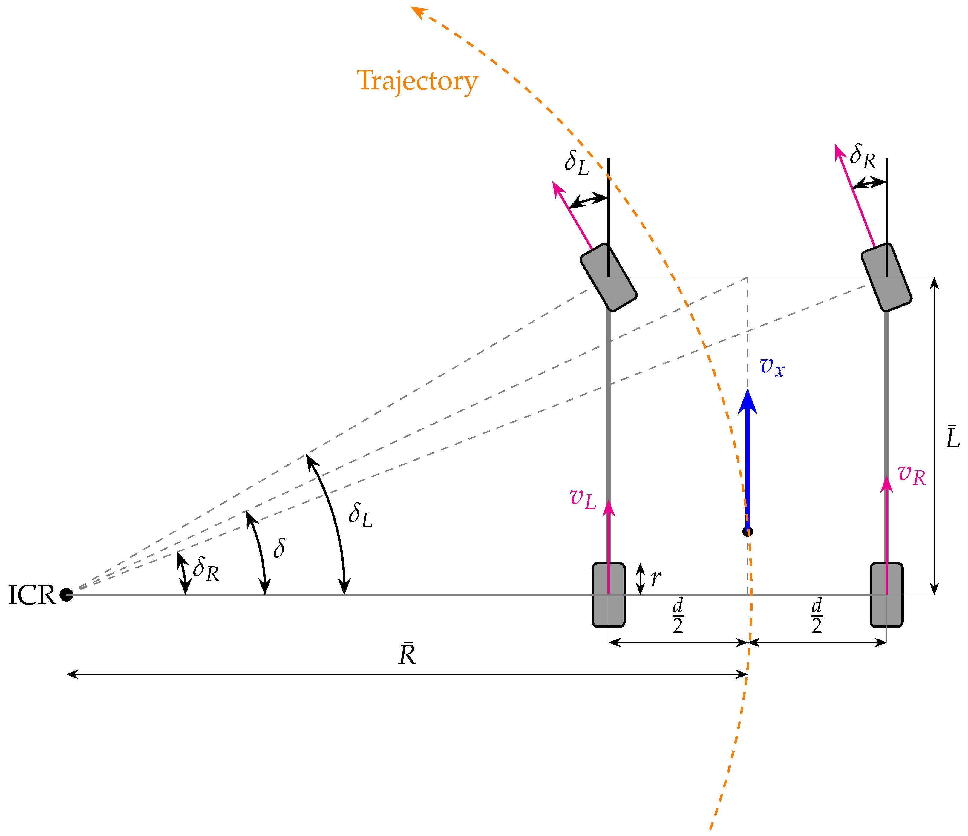
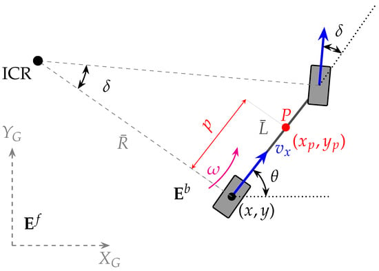
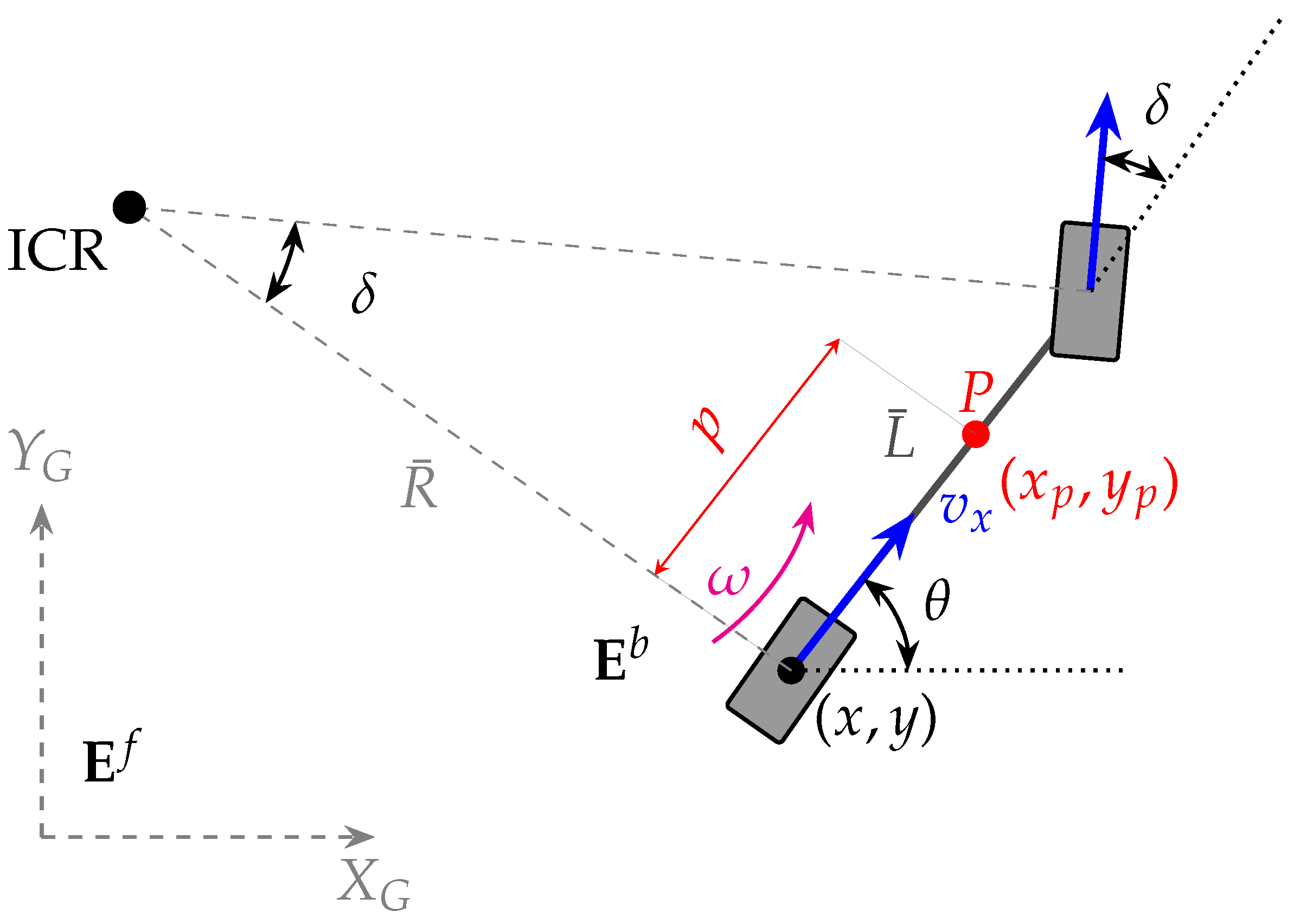
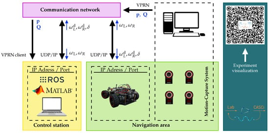
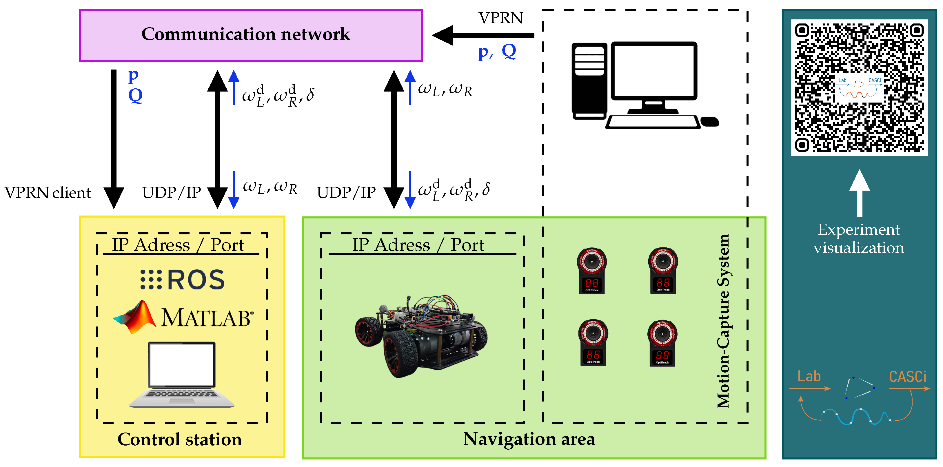
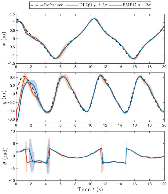
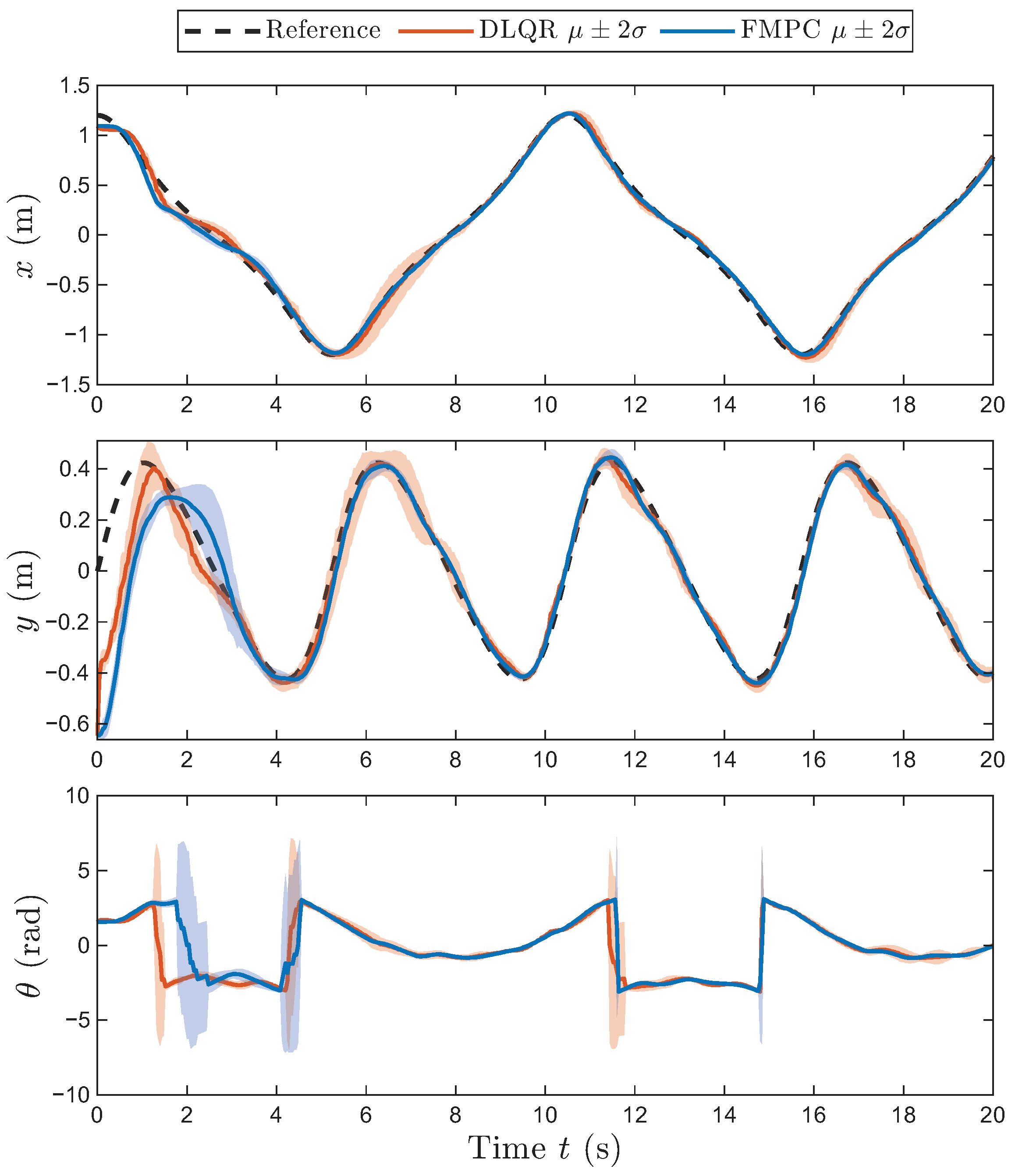
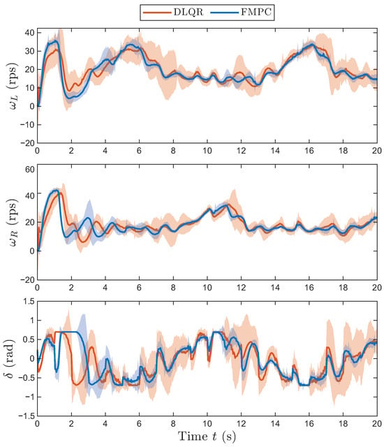
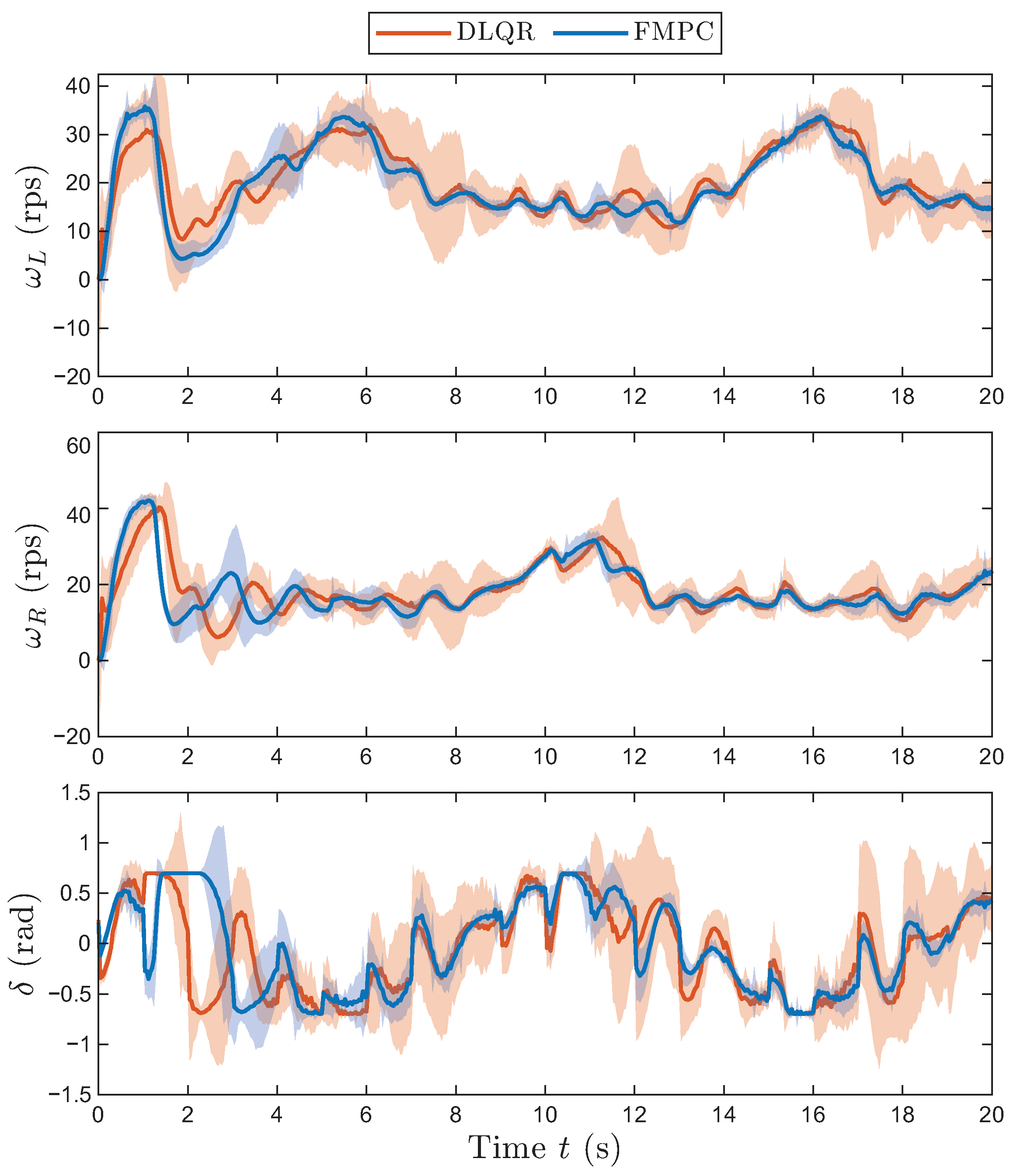
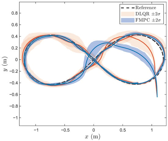
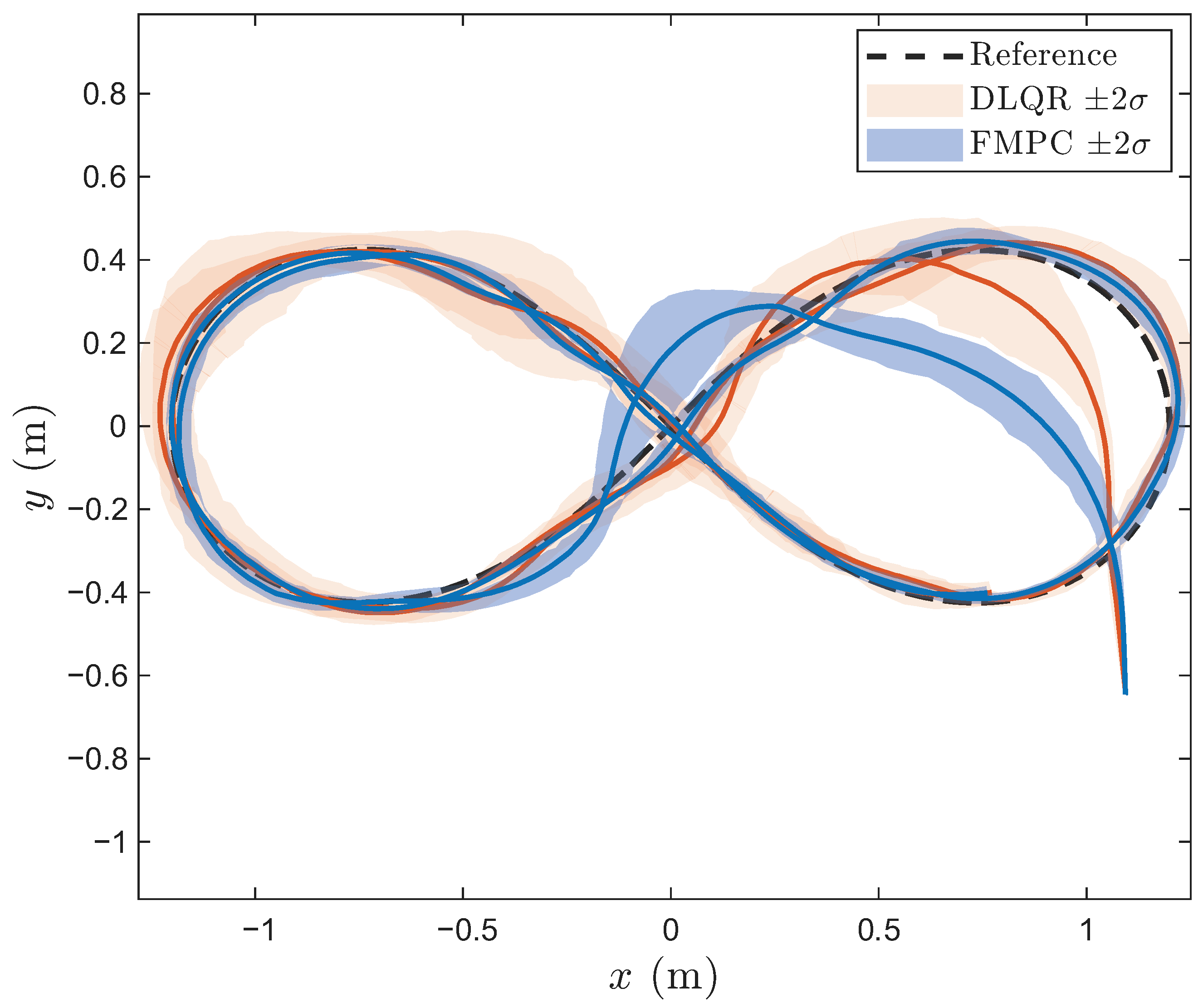
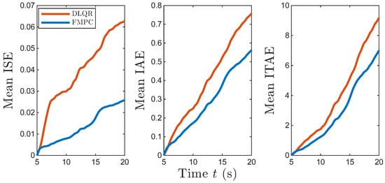
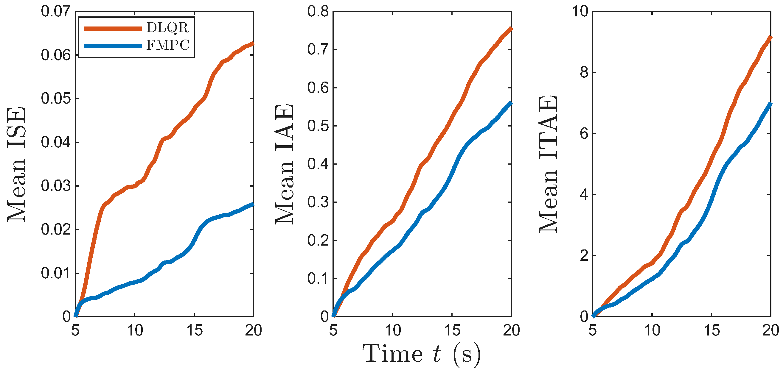
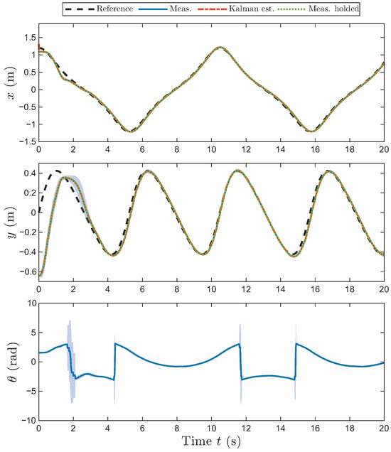
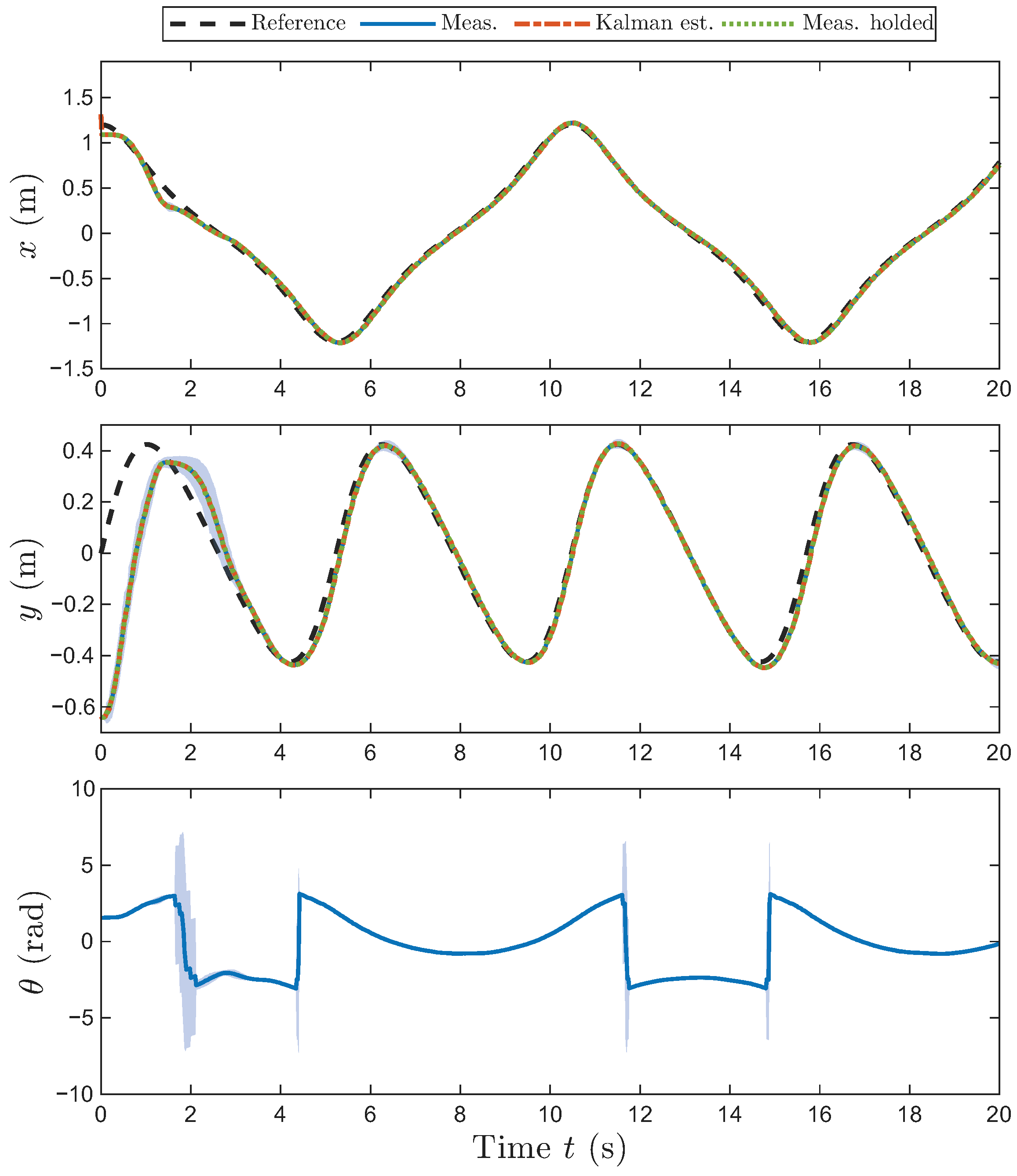
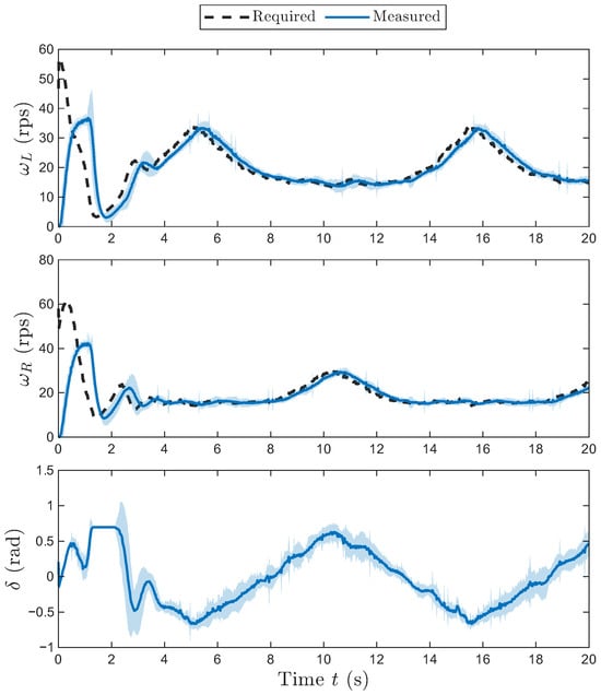
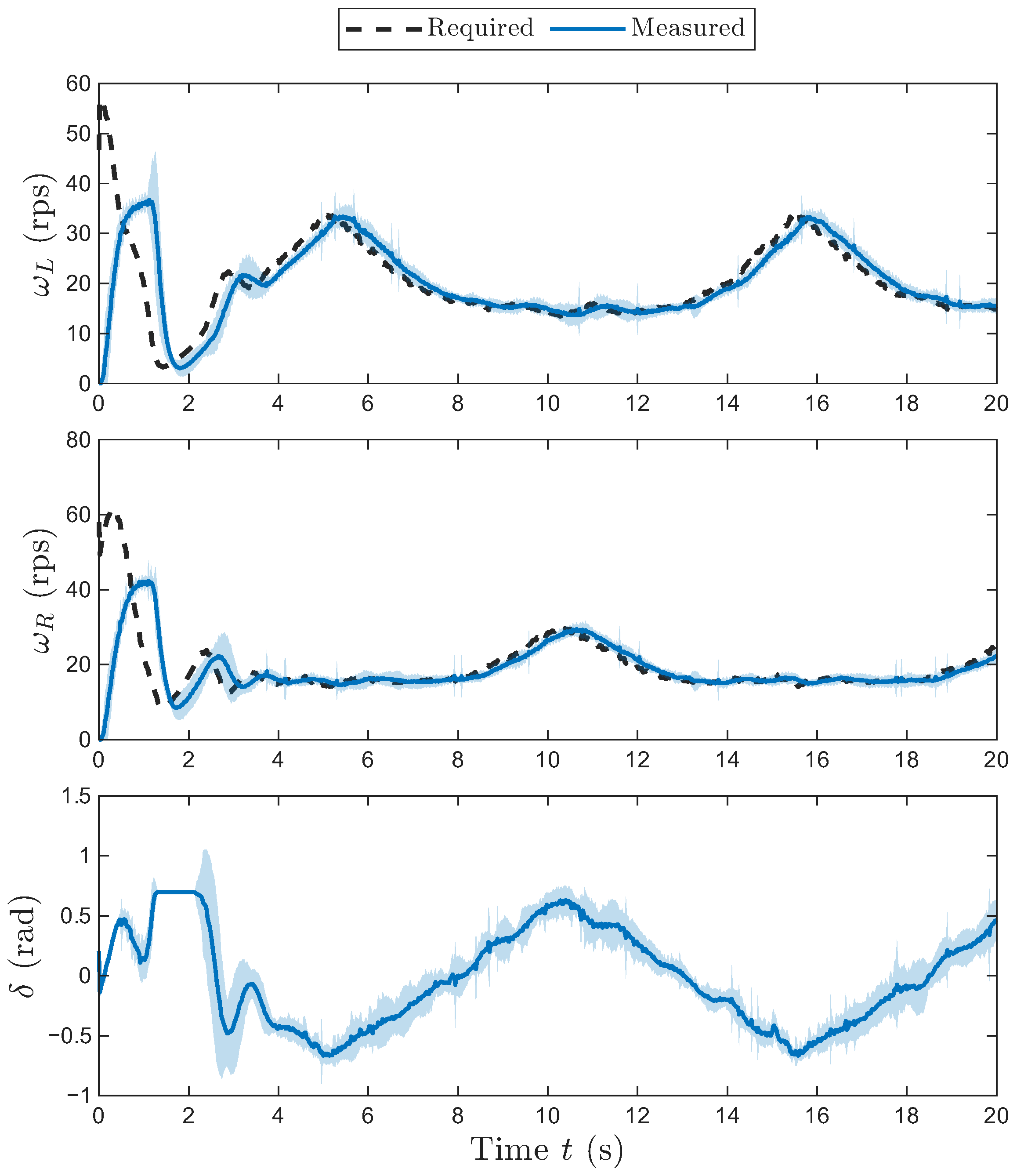
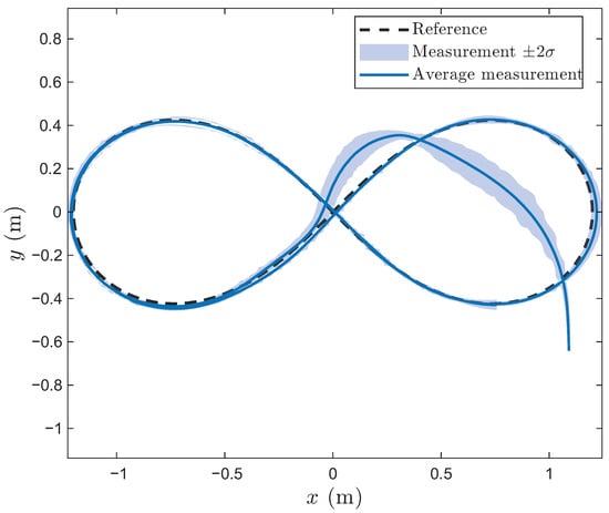
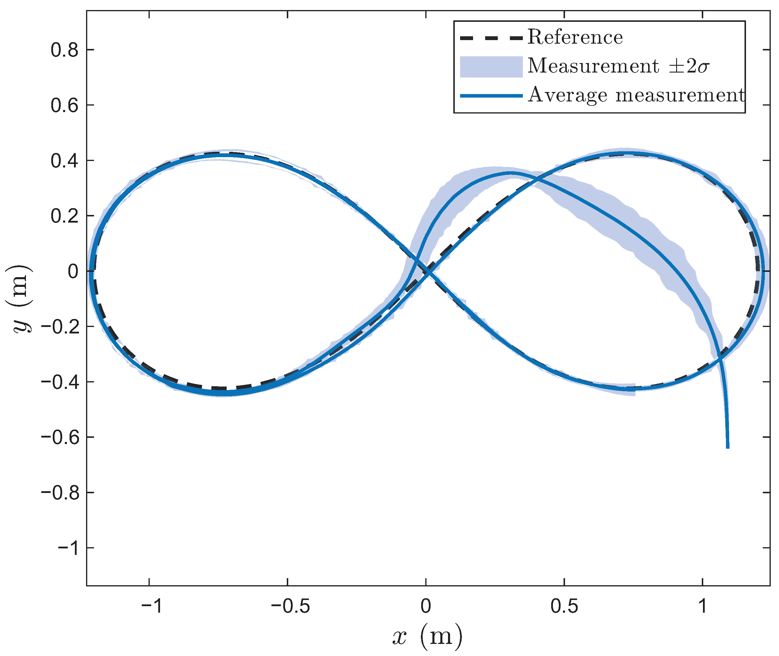
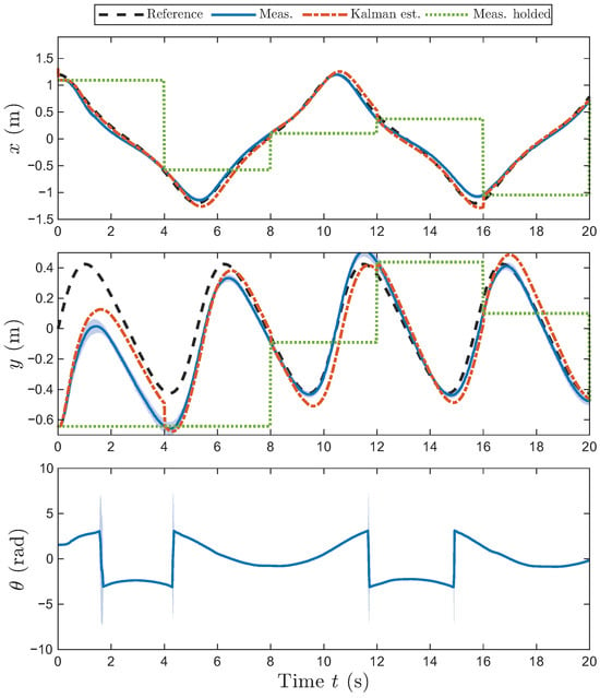
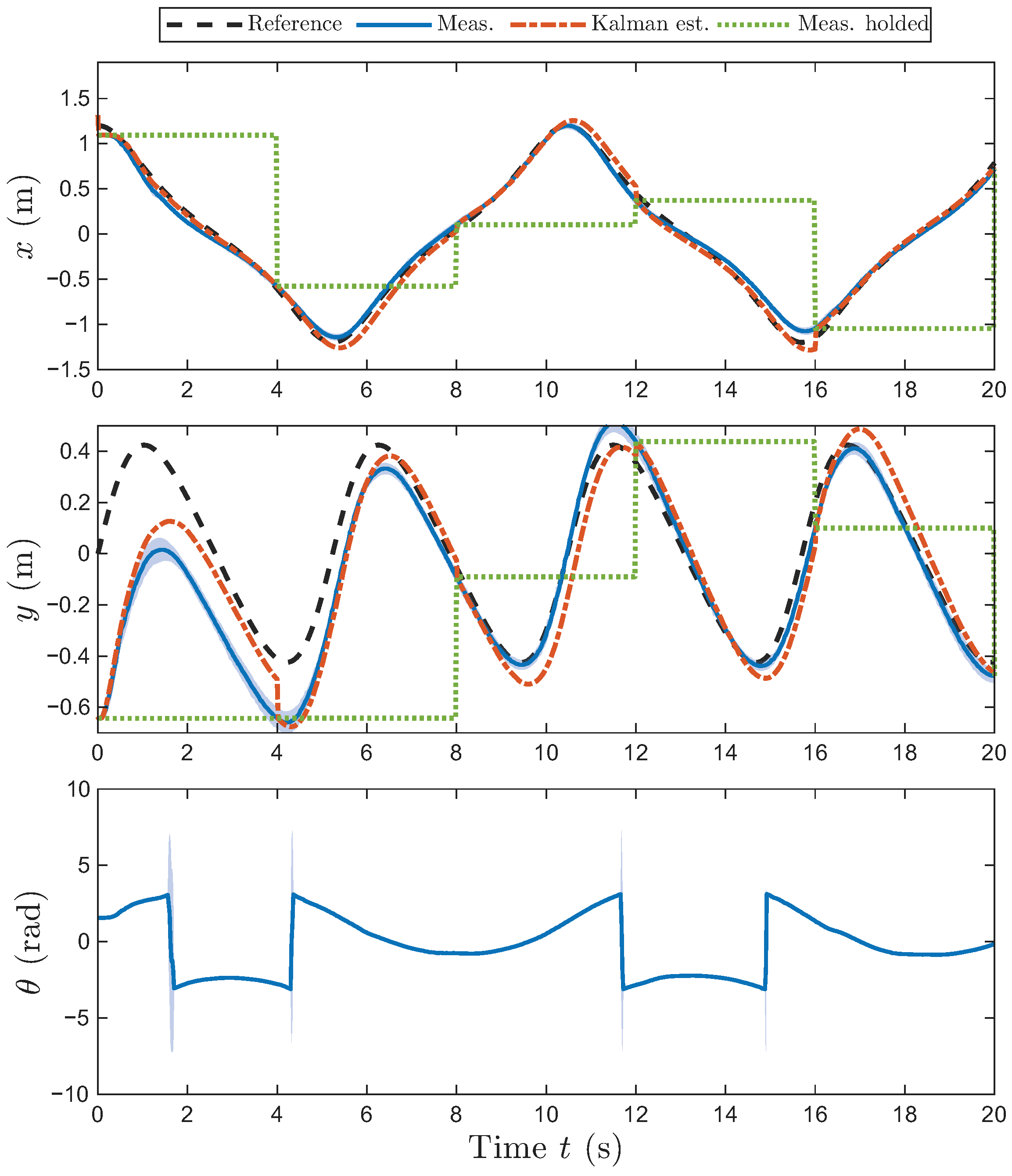
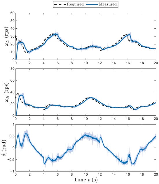
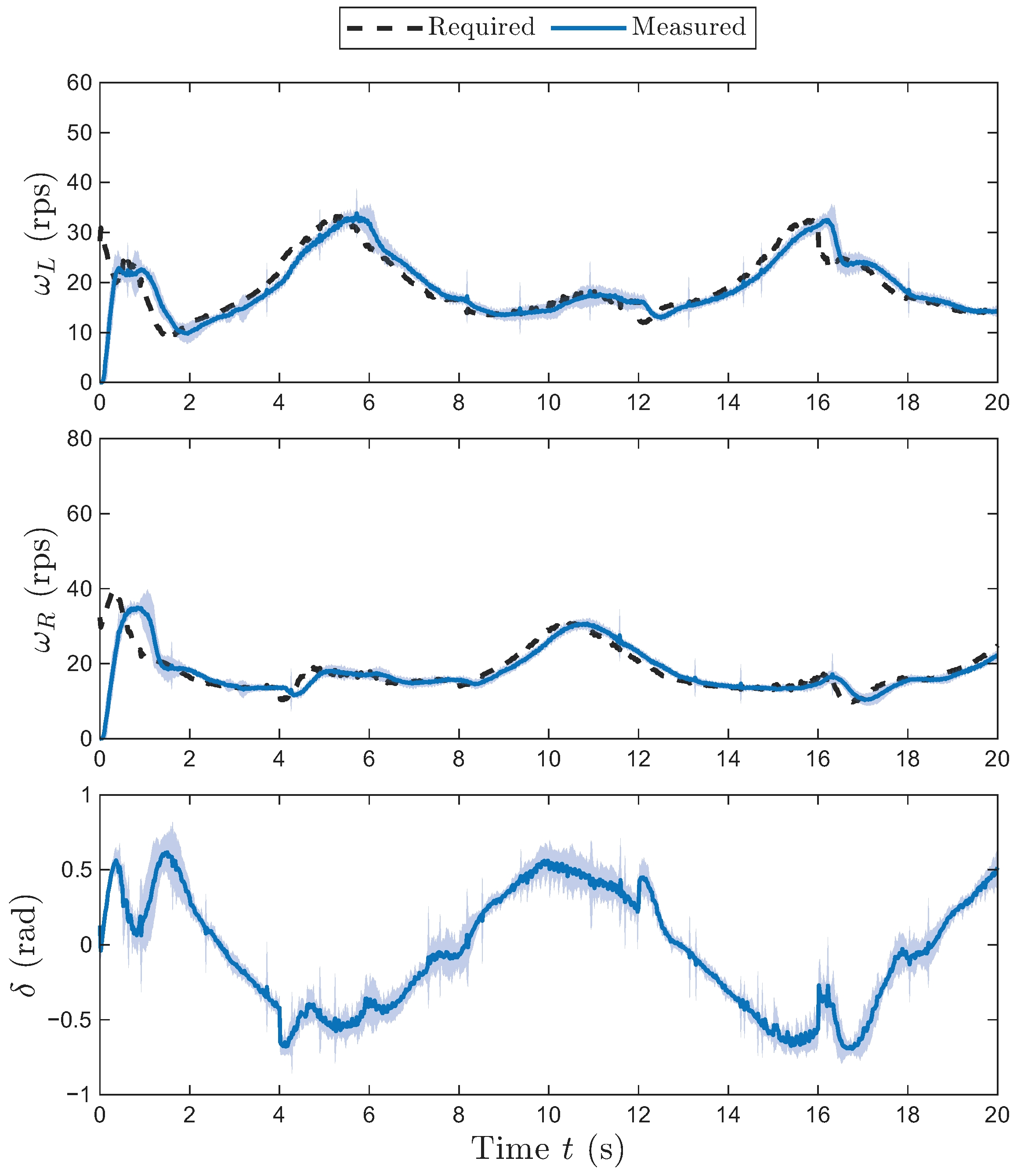
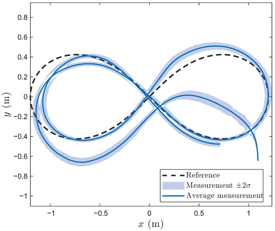
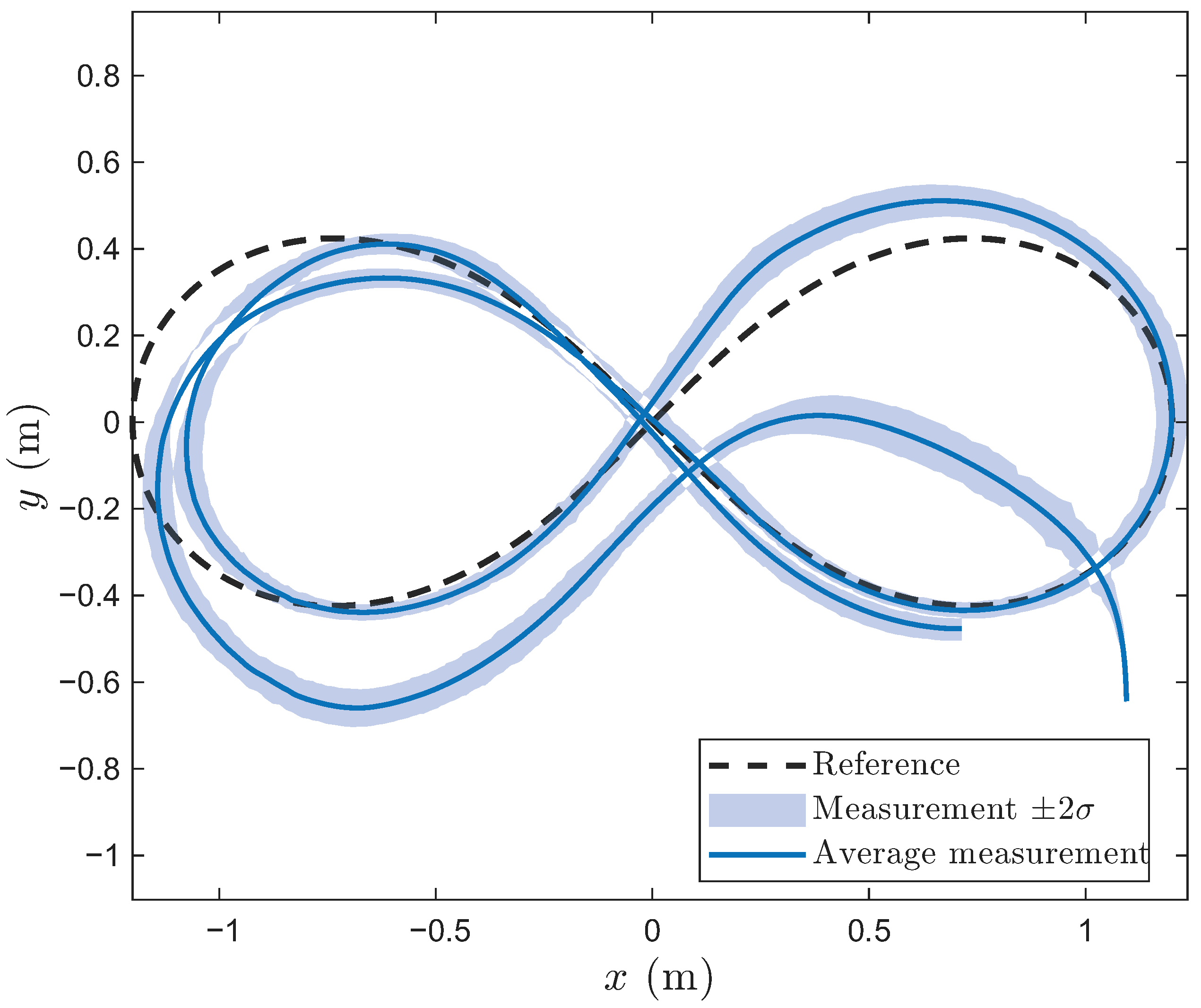
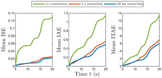
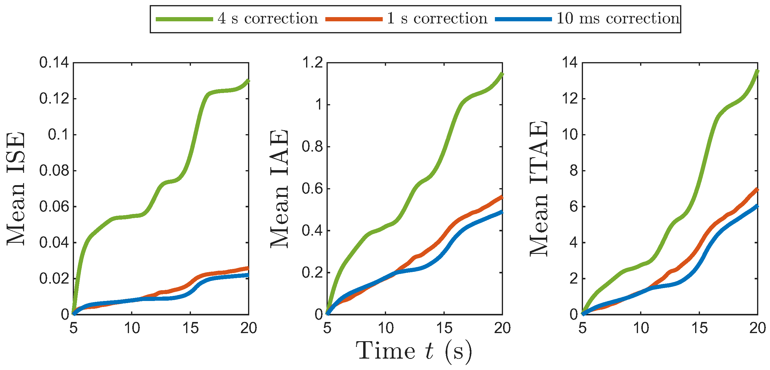
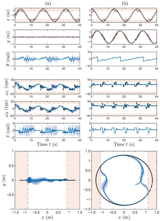
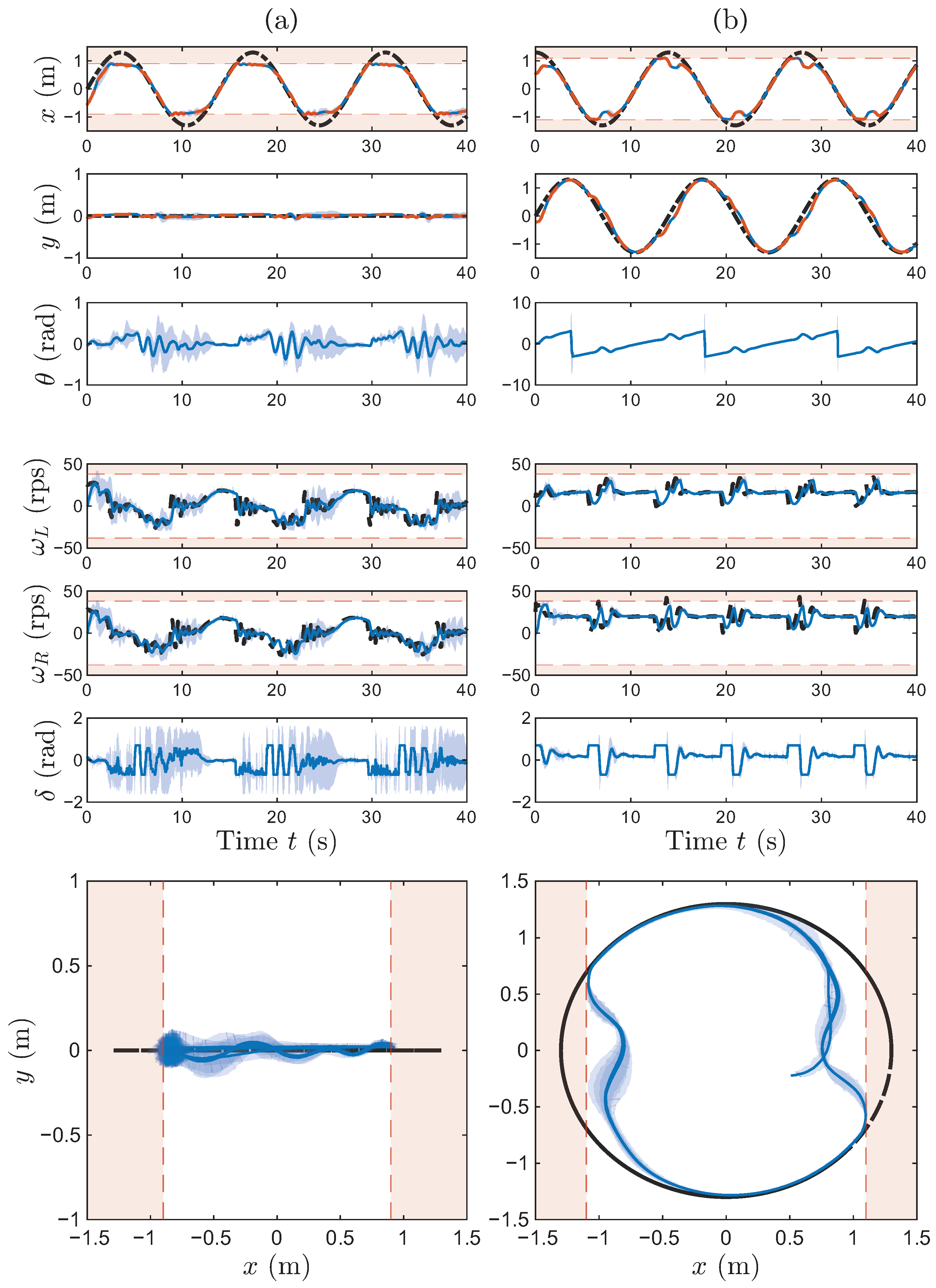
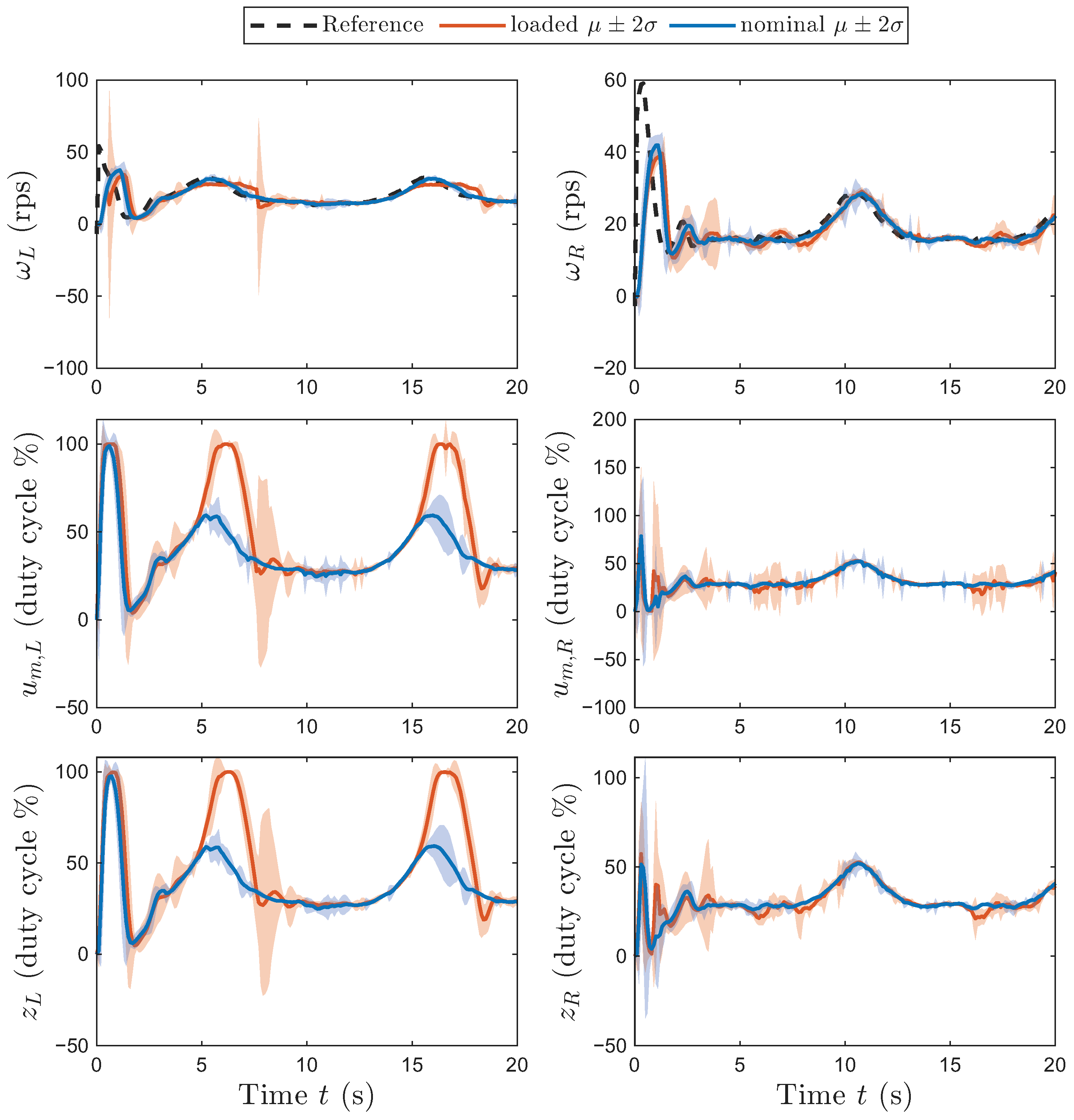
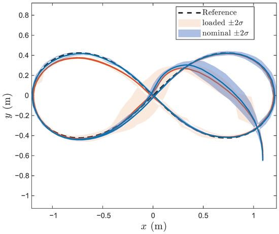
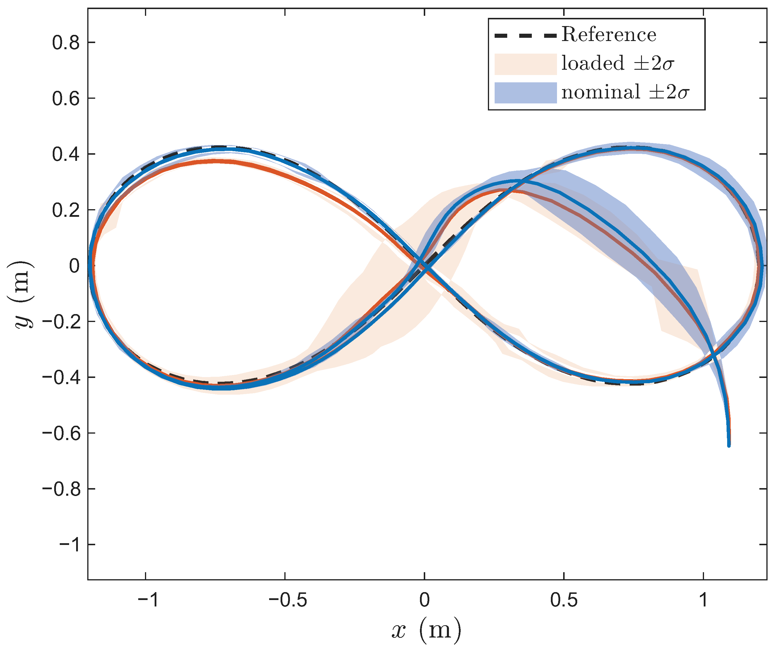
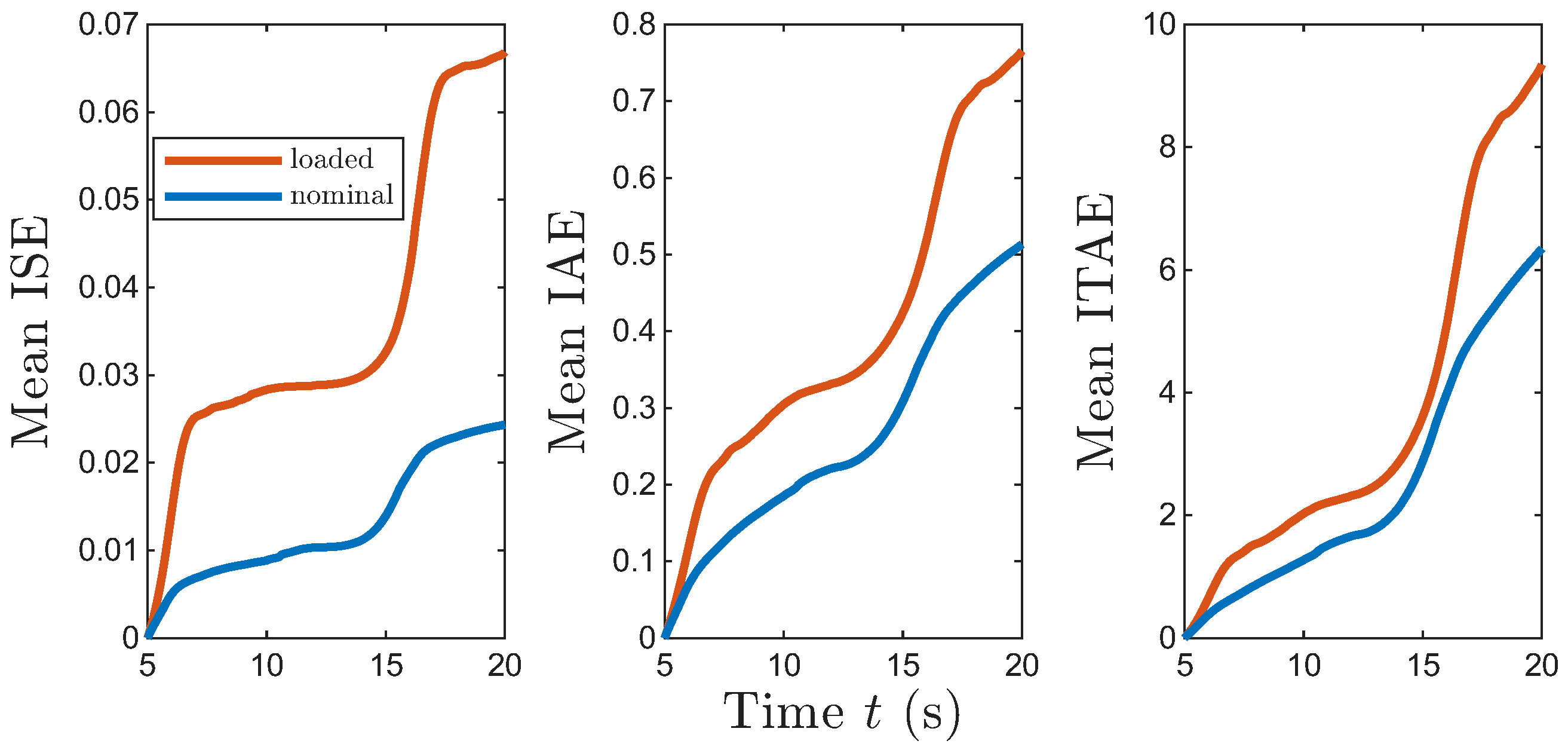
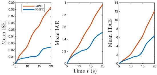
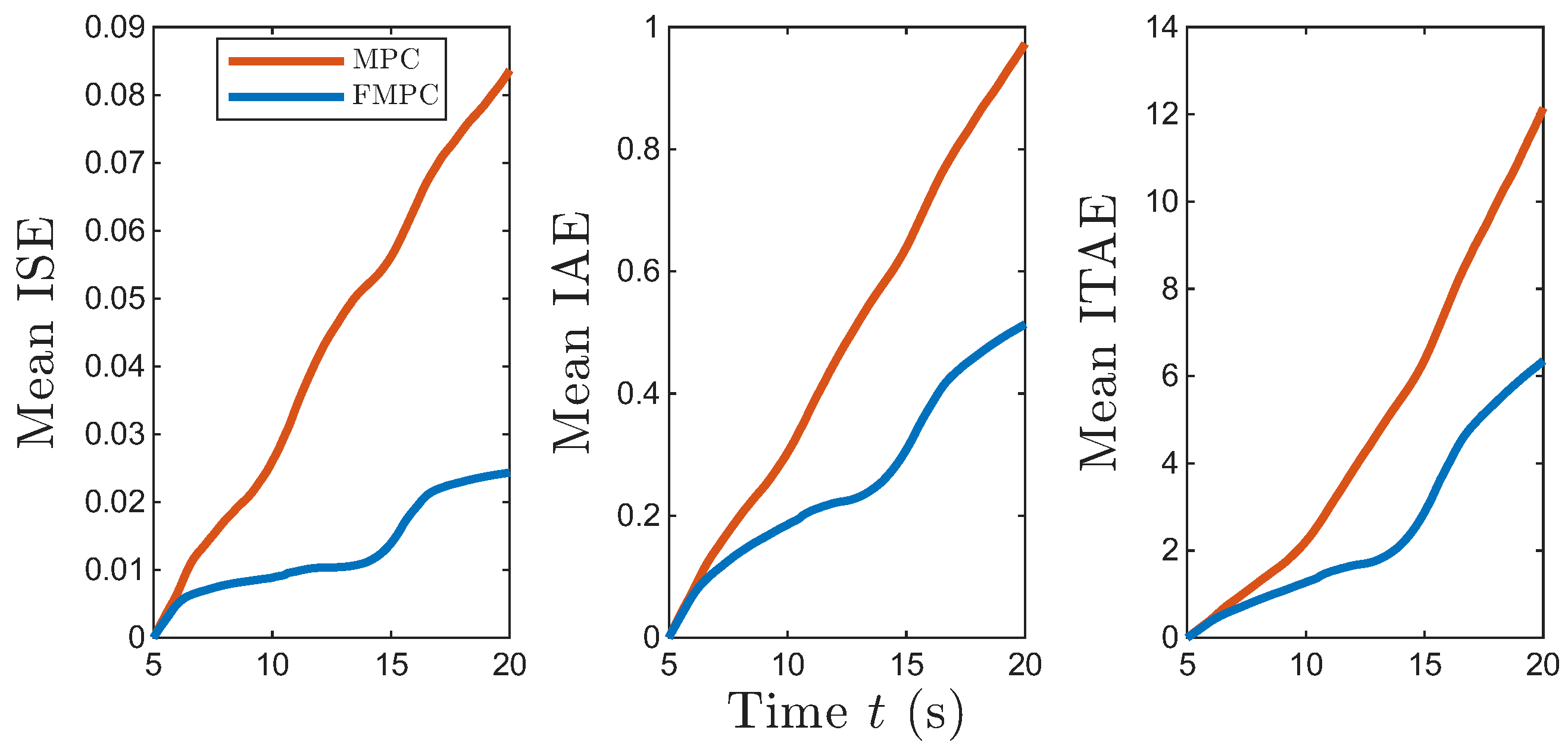
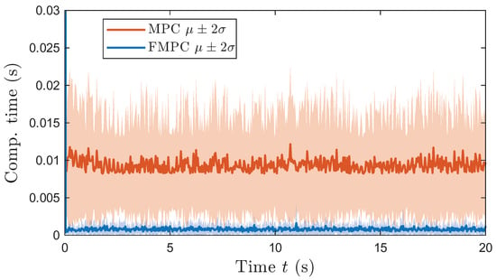
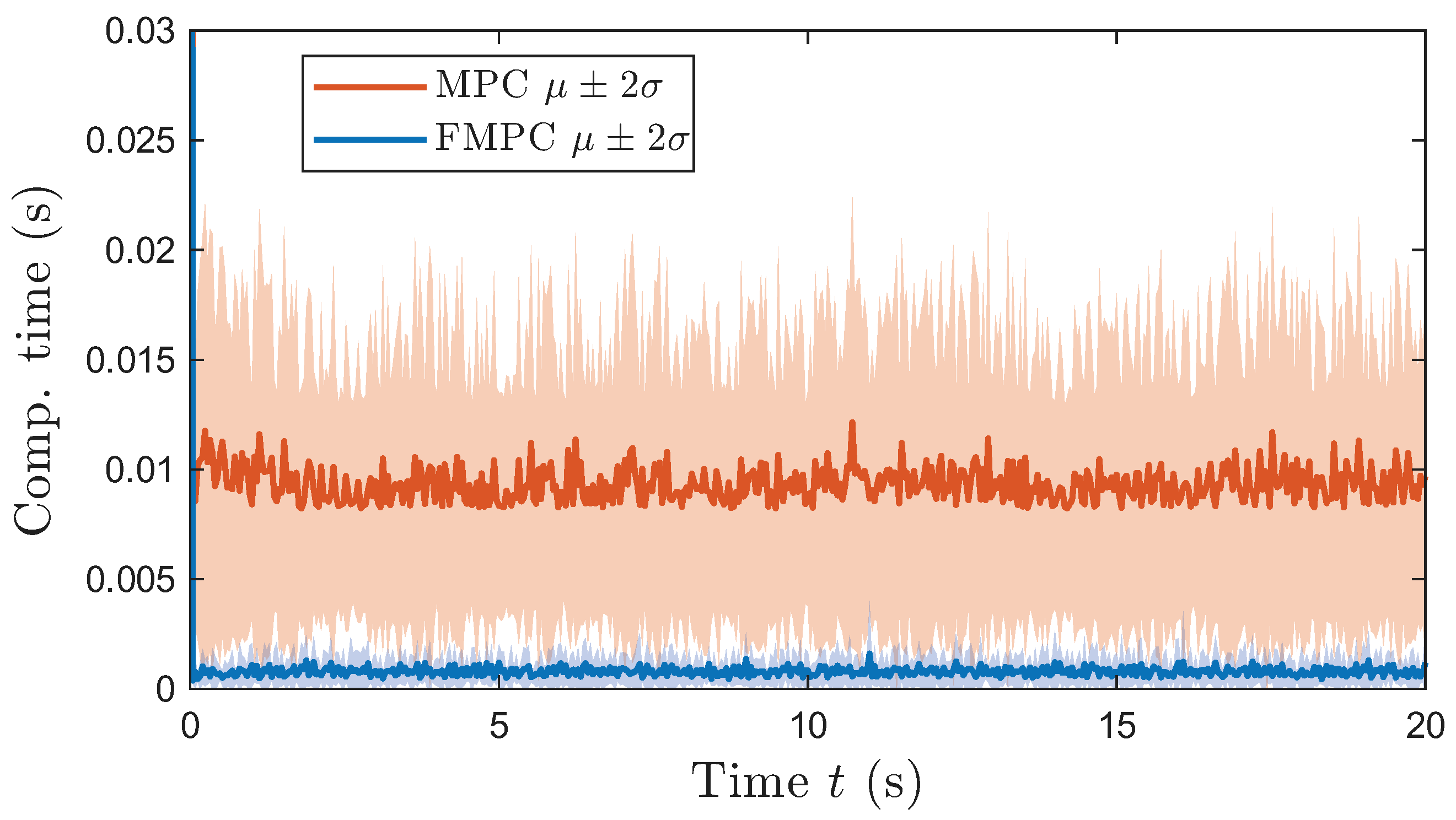
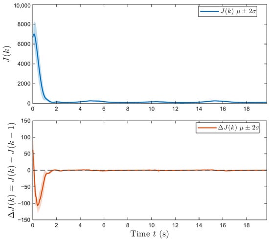
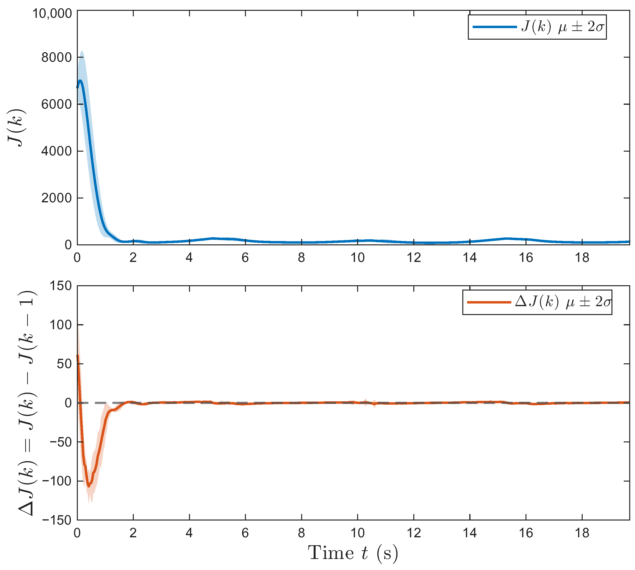

Disclaimer/Publisher’s Note: The statements, opinions and data contained in all publications are solely those of the individual author(s) and contributor(s) and not of MDPI and/or the editor(s). MDPI and/or the editor(s) disclaim responsibility for any injury to people or property resulting from any ideas, methods, instructions or products referred to in the content. |
© 2026 by the authors. Licensee MDPI, Basel, Switzerland. This article is an open access article distributed under the terms and conditions of the Creative Commons Attribution (CC BY) license.