Real-Time Trajectory Replanning and Tracking Control of Cable-Driven Continuum Robots in Uncertain Environments

Abstract

To address trajectory tracking of cable-driven continuum robots (CDCRs) in the presence of obstacles, this paper proposes an integrated control framework that combines online trajectory replanning, obstacle avoidance, and tracking control. The control system consists of two modules. The first is a trajectory replanning controller developed on an improved model predictive control (IMPC) framework. The second is a trajectory-tracking controller that integrates an adaptive disturbance observer with a fast non-singular terminal sliding mode control (ADO-FNTSMC) strategy. The IMPC trajectory replanning controller updates the trajectory of the CDCRs to avoid collisions with obstacles. In the ADO-FNTSMC strategy, the adaptive disturbance observer (ADO) compensates for uncertain dynamic factors, including parametric uncertainties, unmodeled dynamics, and external disturbances, thereby enhancing the system’s robustness and improving trajectory tracking accuracy. Meanwhile, the fast non-singular terminal sliding mode control (FNTSMC) guarantees fast, stable, and accurate trajectory tracking. The average tracking errors for IMPC-ADO-FNTSMC, MPC-FNTSMC, and MPC-SMC are 1.185 cm, 1.540 cm, and 1.855 cm, with corresponding standard deviations of 0.035 cm, 0.057 cm, and 0.078 cm in the experimental results. Compared with MPC-FNTSMC and MPC-SMC, the IMPC-ADO-FNTSMC controller reduces average tracking errors by 29.96% and 56.54%. Simulation and experimental results demonstrate that the designed two-module controller (IMPC-ADO-FNTSMC) achieves fast, stable, and accurate trajectory tracking in the presence of obstacles and uncertain dynamic conditions.

1. Introduction

Compared with classical rigid robotic systems, cable-driven continuum robots (CDCRs) face certain challenges, including reduced bandwidth, nonlinear and coupled dynamics, and increased sensitivity to disturbances. Nevertheless, in unfamiliar and challenging environments, CDCRs offer unique advantages, including flexible deformation, large workspace, and low power consumption. Leveraging these merits, CDCRs have demonstrated broad applicability across multiple areas, including space inspection [1], agricultural harvesting [2], minimally invasive surgery [3], rehabilitation robotics [4], search and rescue operations [5,6], and nuclear reactor inspection and maintenance [7]. To complete these tasks, CDCRs are required to move along the desired trajectory. Therefore, the design of high-performance trajectory tracking controllers for CDCRs has become a research hotspot.

Trajectory replanning for CDCRs has attracted increasing attention due to their high flexibility and complex dynamics. In particular, practical finite-time motion replanning for spacecraft-mounted soft manipulators under dynamic obstacles has demonstrated effective trajectory generation and collision avoidance in challenging environments. In real applications, CDCRs must account for unknown obstacles in complex working spaces [8,9,10], making trajectory replanning essential to ensure safe navigation along a preset trajectory. To address this, Yuan et al. [11] put forward an online minimum-time trajectory replanning algorithm to achieve effective trajectory tracking. Lee et al. [12] designed a path replanning approach for real-time motion to avoid static and dynamic obstacles. However, the above methods do not account for keeping the planned trajectory as close as possible to the preset trajectory, which increases energy and time consumption during trajectory tracking. A path replanning algorithm based on the reinforcement learning method for image segmentation is proposed for trajectory tracking with obstacles and small drifts [13]. However, reinforcement learning methods can not eliminate segmentation errors, which seriously reduces the accuracy of planned trajectories.

To address the trajectory replanning problem in dynamic environments, researchers typically adopt model predictive control (MPC) as the trajectory replanning controller [14]. First, MPC can explicitly handle system constraints, such as actuator limits, kinematic bounds, and obstacle-avoidance requirements, thereby ensuring safe and feasible replanned trajectories. Second, its predictive and optimization-based nature enables anticipation of future system behavior and obstacle motion, leading to smoother and more efficient trajectory adjustments. Third, the receding-horizon framework allows online replanning and rapid adaptation to dynamic environments, making MPC well-suited for real-time trajectory replanning of CDCRs. A nonlinear terminal-free MPC was constructed to solve the problem of discontinuous paths [15]. Wu et al. [16] designed a dynamic nonlinear MPC to avoid obstacles, which can predict the movement trend of obstacles within the predicted range. MPC is adopted for online trajectory replanning to prohibit collisions with moving obstacles [17,18,19]. Liang et al. [20] proposed an economic MPC algorithm for online motion replanning to balance two key factors: efficiency and safety issues. However, the above studies do not consider uncertain dynamic factors of the control system, which affect the accuracy of trajectory tracking.

Although backstepping control is widely used in robotic systems due to its simplicity and capability to handle high-order nonlinear systems, its performance can be degraded by model uncertainties and external disturbances. Uncertain dynamic factors, such as parametric uncertainties, unmodeled dynamics, and external perturbations, pose significant challenges for trajectory tracking controller design and may limit accuracy and stability [21]. Sliding mode control (SMC), a nonlinear method characterized by discontinuous control action, offers strong robustness against such uncertainties and has been widely applied in robotic trajectory tracking [22], missile guidance systems [23], tank fire-control systems [24], advanced motor drive systems [25], and electrical power networks [26]. However, challenges such as chattering, singularity problems, and limited convergence properties continue to restrict its performance [27]. To address the inherent defects and limitations of SMC, scholars have proposed various optimization algorithms to improve its performance. To guarantee convergence within a finite time, terminal sliding mode control (TSMC) was adopted in [28]. Despite its effectiveness, the approach guarantees convergence only to a neighborhood of the origin and may exhibit slower convergence than classical SMC under large initial errors. Furthermore, the presence of fractional power elements and their corresponding negative derivatives renders TSMC susceptible to singularity, while chattering and insufficient tracking accuracy persist. To enhance convergence efficiency, Zhong et al. [29] proposed a fast terminal sliding mode control (FTSMC) strategy, which increases the convergence rate after the system reaches the sliding manifold. However, the issues of chattering and singularity are still not completely addressed. Shao et al. [30] further introduced an adaptive recursive integral terminal sliding mode controller (ARITSMC) to enhance both convergence rate and tracking precision, thereby strengthening the robustness of the control system. Nevertheless, the use of a sign function in the reaching control term can exacerbate chattering effects. SMC arises from discontinuous switching in the control law. When the system state approaches the sliding surface, the control input switches rapidly, causing high-frequency oscillations. This reduces trajectory tracking accuracy and increases actuator load [31]. Therefore, it is necessary to suppress chattering in SMC. Liu et al. [32] propose an adaptive neural network-based fixed-time control strategy for robots with input saturation and prescribed performance, ensuring rapid and bounded convergence. Reference [33] develops an adaptive neural network-based fixed-time trajectory tracking control method for robotic systems, demonstrating robust performance under uncertain dynamics.

Building on existing research, a two-module trajectory replanning and tracking controller is developed for CDCRs with uncertain dynamics to achieve improved performance in challenging operational conditions. The overall scheme integrates an IMPC-based replanning module with an adaptive disturbance-observer-assisted fast non-singular terminal sliding mode controller (ADO-FNTSMC). The major contributions of this study are as follows:

(1)

By updating the trajectory in real time, the IMPC-based trajectory replanning controller avoids collisions with both static and dynamic obstacles, ensures safe and flexible operation under system constraints, and mitigates the local optimality problem inherent in conventional MPC via rolling-horizon optimization.

(2)

Compared with conventional SMC, TSMC, and FTSMC, the FNTSMC not only mitigates chattering and singularity issues but also improves tracking accuracy and stability.

(3)

The proposed ADO estimates uncertain dynamics in real time and incorporates compensation into the control law, thereby enhancing trajectory tracking and system robustness.

(4)

To refine the estimation of uncertain dynamic disturbances, an improved grey wolf optimizer (IGWO) is applied within the ADO, exploiting the grey wolves’ exploration strategy, thereby further improving trajectory tracking performance.

The rest of this paper is structured as follows: Section 2 establishes the CDCR model. Section 3 elaborates on the trajectory replanning controller, and Section 4 discusses the trajectory tracking controller. Simulation investigations are reported in Section 5, and Section 6 provides experimental validation of the proposed obstacle-avoidance and tracking control framework. The conclusions are summarized in Section 7.

2. Problem Formulation

2.1. Kinematic Modeling

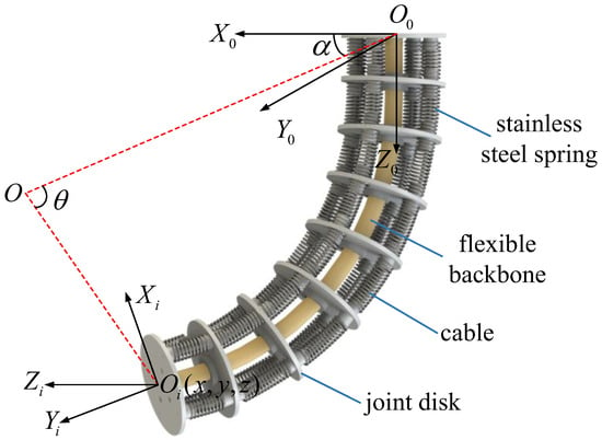
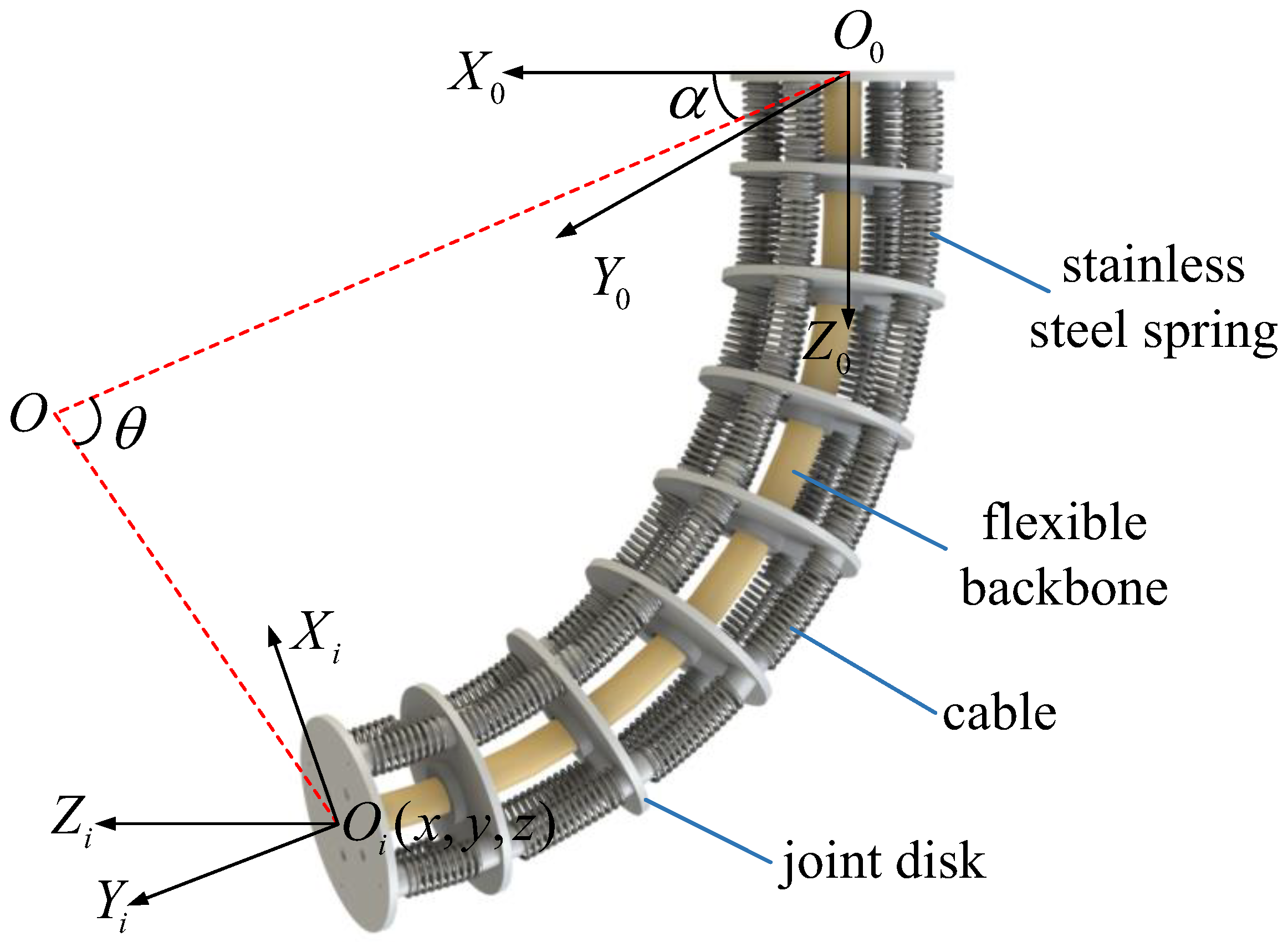
The joint space bending angle θ and rotation angle α are controlled through adjustments of the CDCR’s cable lengths (as presented in Figure 1). The corresponding workspace position vector is denoted as w = [x, y, z]^T, and the joint space configuration vector is h = [θ, α]^T. The CDCR has a total length of d = 40 cm. Its kinematics can be formulated as follows:

$$w=p(h)={\left[{\displaystyle \frac{d}{\theta }}\cos \alpha \left(1-\cos \theta \right)\hspace{1em}{\displaystyle \frac{d}{\theta }}\sin \alpha \left(1-\cos \theta \right)\hspace{1em}{\displaystyle \frac{d}{\theta }}\sin \theta \right]}^{\mathrm{T}}$$

(1)

where p(h) corresponds to the transformation vector.

Figure 1. Schematic illustration of the CDCR geometry.

2.2. Dynamic Modeling

Using Lagrange’s approach, the dynamics of the CDCR are expressed as

$$Q(h)\ddot{h}+F(h,\dot{h})\dot{h}+E(h)+{\psi }_{\mathrm{f}}=\psi$$

(2)

In this formulation, $\dot{h}$ and $\ddot{h}$ stand for the velocity and acceleration vectors of the CDCR joint angles. $Q(h)$ is the inertia matrix, $F(h,\dot{h})$ denotes the Coriolis and centrifugal forces, $E(h)$ is the gravitational component, ${\psi }_{\mathrm{f}}$ accounts for joint friction, and $\psi$ represents the applied joint torques.

However, $Q(h)$, $F(h,\dot{h})$, $E(h)$ cannot be accurately obtained, which are assumed to satisfy:

$$\left\{\begin{array}{l}Q(h)=\widehat{Q}(h)+\Delta Q(h)\hfill \\ F(h,\dot{h})=\widehat{F}(h,\dot{h})+\mathsf{\Delta }F(h,\dot{h})\hfill \\ E(h)=\widehat{E}(h)+\mathsf{\Delta }E(h)\hfill \end{array}\right.$$

(3)

where $\widehat{Q}(h)$, $\widehat{F}(h,\dot{h})$, and $\widehat{E}(h)$ are estimations of $Q(h)$, $F(h,\dot{h})$, and $E(h)$, respectively. $\mathsf{\Delta }Q(h)$, $\mathsf{\Delta }F(h,\dot{h})$, and $\mathsf{\Delta }E(h)$ are system uncertainties. Thus, Equation (3) can be further formulated as

$$\widehat{Q}(h)\ddot{h}+\widehat{F}(h,\dot{h})\dot{h}+\widehat{E}(h)=\psi -X(h,\dot{h},\ddot{h})$$

(4)

$X(h,\dot{h},\ddot{h})$ is the systematic error term, which can be defined as

$$X(h,\dot{h},\ddot{h})={\psi }_{\mathrm{f}}+\mathsf{\Delta }Q(h)\ddot{h}+\mathsf{\Delta }F(h,\dot{h})\dot{h}+\mathsf{\Delta }E(h)$$

(5)

The error between the desired and actual trajectory is expressed as

$$e=h-h_{\mathrm{d}}$$

(6)

where $h_{\mathrm{d}}$ is defined as the desired position vector of the CDCR. Therefore, Equation (7) can be expressed as

$$\widehat{Q}(h)\ddot{e}=\psi -X(h,\dot{h},\ddot{h})-\widehat{F}(h,\dot{h})\dot{h}-\widehat{E}(h)-\widehat{Q}(h){\ddot{h}}_{\mathrm{d}}$$

(7)

3. Trajectory Replanning

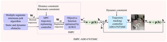
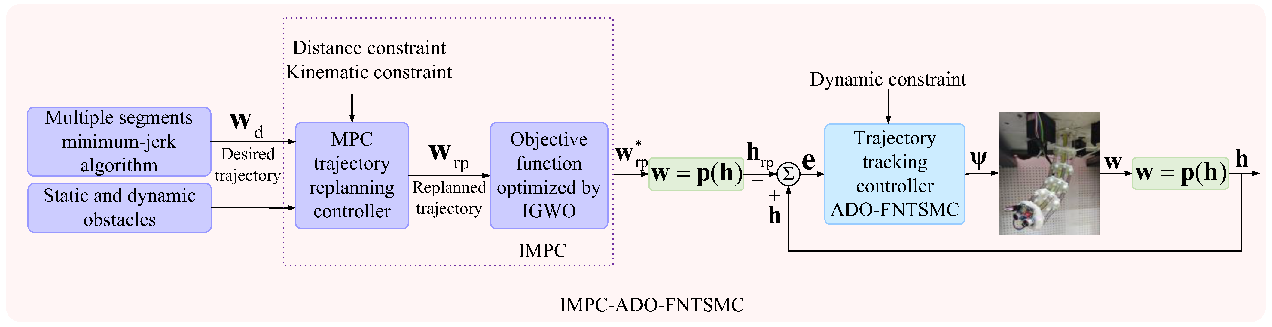
This section comprises a trajectory-generation controller and a real-time trajectory-replanning controller based on MPC. The trajectory-generation controller is constructed using a minimum-jerk algorithm with multiple segments, which mitigates the effect of jerk on trajectory smoothness. The MPC trajectory-replanning controller is designed for obstacle avoidance, offering safe, adaptive, and flexible avoidance capabilities in the presence of static and dynamic obstacles. The trajectory-tracking controller then follows the trajectory generated by the replanning module, enabling safe and flexible obstacle avoidance and high-performance trajectory tracking. The schematic of the two-module trajectory replanning and tracking framework is depicted in Figure 2.

Figure 2. The schematic of the two-module trajectory replanning and tracking framework.

3.1. Trajectory Generation

The minimum-jerk algorithm is adopted for trajectory generation to improve the smoothness of the trajectory [34]. The newly generated trajectory consists of multiple trajectory segments, with each segment represented by the polynomial below:

$$S(t)={\displaystyle \sum _{i=1}^{n}f}{w}_{i,t}(t)$$

(8)

$S(t)$ is the trajectory generated within the single trajectory segment at time t, $w_{i,t}(t)$ is the position vector of i point at time t, n is the number of point vectors, and f is the weight coefficient.

The minimum-jerk algorithm for a single trajectory segment is designed as

$$F(T_j)={\displaystyle {\int }_{T_j}^{T_{j+1}}{S}^{(3)}{(t)}^2}dt$$

(9)

where $F(T_j)$ represents the jth segment trajectory at initial time T_j and final time T_j+1. The optimization problem of whole trajectory generation can be expressed as

$$\begin{array}{l}\underset{f}{\min }{\displaystyle \sum _{j=1}^{m}F(T_j)}\\ s\mathrm{.}t:{\dot{w}}_{\min }\le \dot{w}\le {\dot{w}}_{\max }\\ {\ddot{w}}_{\min }\le \ddot{w}\le {\ddot{w}}_{\max }\\ l_{t,j}=l_{0,j+1}\\ S(t)\in K\\ i=0,1,2,\dots ,n\\ j=0,1,2,\dots ,m\end{array}$$

(10)

where $l_{t,j}$ corresponds to the derivatives at the termination of the jth segment, and $l_{0,j+1}$ indicates the derivatives at the initiation of the following segment. K is the feasible domain of the CDCR. The time t_j for generating the jth segment trajectory is devised as

$$t_j=T_{j+1}-T_j={\displaystyle \frac{{\dot{w}}_{\max }^2+q_j{\ddot{w}}_{\max }}{{\ddot{w}}_{\max }{\dot{w}}_{\max }}}$$

(11)

where q_j refers to the distance from the beginning to the end of the jth segment of the trajectory.

3.2. Trajectory Replanning

Obstacle locations are acquired using an HC-SR04 ultrasonic sensor mounted on the CDCR’s end-effector. To maintain a safe separation between the CDCR and obstacles, a cost function $H_{ob,k}$ is incorporated as a soft constraint in the MPC trajectory replanning controller. The function $H_{ob,k}$ is formulated as follows [35]:

$$H_{\mathrm{ob},k}={\displaystyle \frac{G_{\mathrm{ob}}}{{d_{k,0}}^2+\tau }}$$

(12)

where $G_{\mathrm{ob}}$ represents the weight factor, (x_k, y_k, z_k) denotes the CDCR end-effector coordinates, ($x_0$, $y_0$, $z_0$) specifies the point on the obstacle nearest to the end-effector, $d_{k,0}=\sqrt{{(x_k-x_0)}^2+{(y_k-y_0)}^2+{(z_k-z_0)}^2}$. $\tau$ is a small positive value introduced to avoid division by zero.

The replanned trajectory is designed to quickly align with the desired trajectory, minimizing both deviation and obstacle collisions, thereby achieving efficient energy use.

The MPC trajectory replanning controller is constructed as

$$\underset{u}{\min }{\displaystyle \sum _{p=1}^{N_r}{‖w_{\mathrm{rp}}(k+p)-w_{\mathrm{d}}(k+p)‖}_Q^2}+\sum _{p=0}^{N_s-1}{‖\Delta u(k+p)‖}_R^2+\sum _{p=1}^{N_r}\sum _{h=1}^{N_{\mathrm{ob}}}{H}_{\mathrm{ob},k,h}$$

(13)

where Nr and Ns represent the domain used for prediction and control. Q and R are matrices that determine the weight of position increments and control increments, respectively. $w_{\mathrm{rp}}$ and $w_{\mathrm{d}}$ denote the position vector of the replanned trajectory and desired trajectories. $\Delta u$ is the control increment.

The hard constraints of safe distance between the end-effector for the CDCR and obstacles are defined as

$$d_{k,0}\ge d_{k,0,\min }$$

(14)

where $d_{k,0,\min }$ indicates the minimum safe distance between the end-effector and the closest obstacle location.

The kinematic constraints are defined as

$$\begin{array}{l}{u}_{\min }(k+p|t)\le u(k+p|t)\le u_{\max }(k+p|t)\hspace{1em}p=0,1,\cdots N_r-1\\ t=\mu T_s, \stackrel{\min }{\mu }=1,2,\cdots {\mu }_{\max }\end{array}$$

(15)

where T_s is the sampling period, and ${\mu }_{\max }$ is related to the delay of the sensor and the response time of the planning controller.

Stability constraint is defined as

$${‖w_{\mathrm{rp}}(k+p)-w_{\mathrm{d}}(k+p)‖}_Q^2=0\hspace{1em}p=0,1,\dots N_r$$

(16)

The MPC trajectory replanning controller is designed for obstacle avoidance to enhance safety, which benefits from MPC’s rolling optimization. IGWO is developed to improve the trajectory replanning performance of MPC, ensuring that the replanned trajectory meets the system’s safety distance and kinematic constraints.

The grey wolf optimizer (GWO) is mathematically described as follows:

$$\left\{\begin{array}{c}{S}_{wp}=\left|L{P}_{lp}(t)-P_{W_d}(t)\right|\\ P_m(t+1)={\displaystyle \frac{1}{3}}{\displaystyle \sum _{lp=W_a,W_b,W_c}(P_{lp}(t)-M{S}_{wp})}\\ M=2r{U}_1-r\\ L=2U_2\end{array}\right.$$

(17)

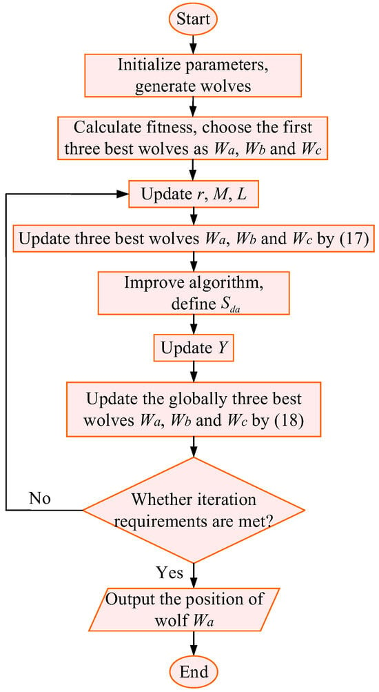
The wolves W_a, W_b, and W_c denote the top three solutions. In each iteration, they are reselected according to the performance ranking of the feasible solutions. Wolf W_d approaches the prey position under the guidance of wolf W_a, W_b, and W_c. The wolves’ positions are marked as $P=(p^1,p^2,p^3,\dots p^D)$, which represents the replanned trajectory $w_{\mathrm{rp}}$ of the MPC trajectory replanning controller. t is the current iteration, $P_{lp}(t)$ corresponds to the prey location, S_wp measures the distance from wolf W_d to the prey, and $P_m(t+1)$ specifies the subsequent position for encircling the prey. The guidance coefficients are M and L, $U_1$ and $U_2$ represent random numbers between 0 and 1, and r is a control parameter varying from 0 to 2.

As shown in Equation (17), a linear decrease in the control parameter r may cause wolf W_d to converge prematurely to a local optimum when approaching wolves W_a, W_b, and W_c. To mitigate this problem, IGWO is developed by integrating the detection mechanism inspired by the artificial bee colony (ABC) algorithm into the conventional GWO framework. It is obvious that $w_{rp}^{\ast }$ generated by IGWO is more accurate. According to Equation (17), the detection mechanism of wolf W_d is formulated as

$$P_{W_d}^{new}(\varpi )=P_{W_d}+Y{S}_{da}\hspace{1em}\varpi \in \left\{1,2,\dots ,M\right\}$$

(18)

where $P_{W_d}^{new}(\varpi )$ and $P_{W_d}$ denote the new and current positions of wolf W_d, respectively. The number of investigation attempts is M, and $S_{da}$ represents the distance between W_d and the top-ranking wolves (W_a, W_b, W_c), which serves as the search radius. The variable Y takes random values in the range [−1, 1]. During the investigation, if W_d finds an updated position approaching the prey, it moves there; otherwise, it stays at its previous position.

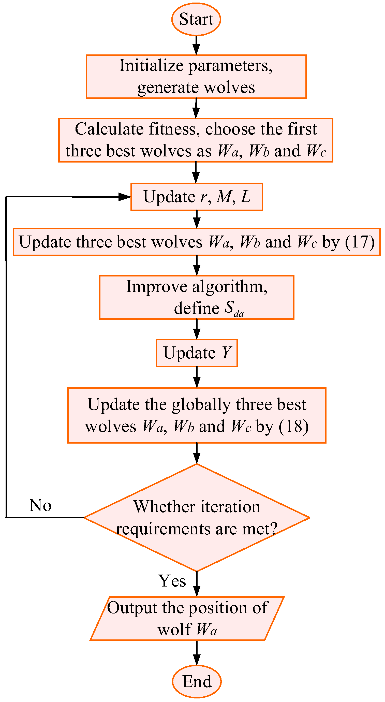
Figure 3 depicts the flowchart of the IGWO algorithm.

Figure 3. The flowchart of the IGWO.

In an environment with dynamic obstacles, the proposed algorithm predicts their motion trends using the MPC’s rolling optimization. By incorporating these predictions into trajectory replanning, the system can proactively adjust its trajectory to avoid collisions while maintaining smooth, accurate motion. For static obstacles, the ultrasonic sensor provides sufficient position information, so no additional prediction is needed, thereby optimizing computational resources.

4. Dynamic Trajectory Tracking Controller Design

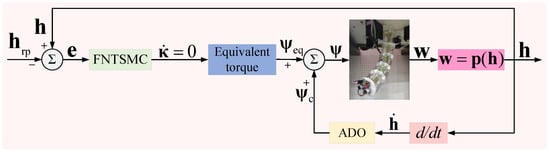
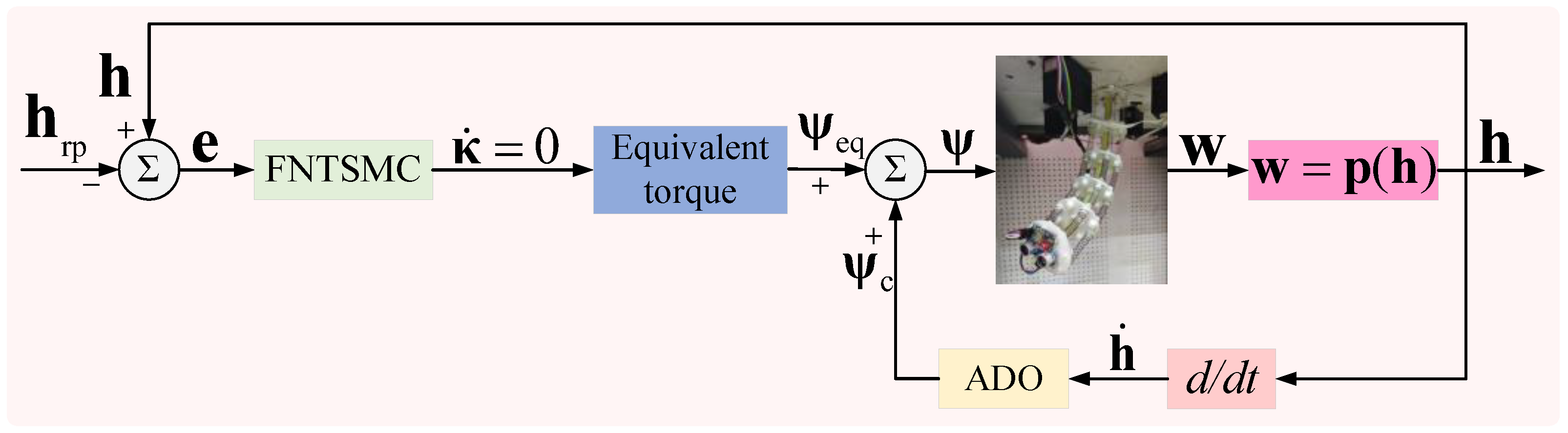
An ADO-FNTSMC, consisting of an FNTSMC and an ADO, is presented in this section to boost CDCR trajectory tracking. The ADO-FNTSMC structure is depicted in the block diagram of Figure 4. The FNTSMC offers strong capabilities in chattering suppression, non-singularity, and rapid convergence to zero. The ADO estimates uncertain dynamic effects and applies compensation to the control signal, enhancing both tracking accuracy and system robustness. An IGWO that integrates grey wolf scouting behavior is applied within the ADO to achieve global-optimal estimation of dynamic uncertainties, mitigating the risk of local minima.

Figure 4. The block diagram of the ADO-FNTSMC for the CDCR.

4.1. FNTSMC Design

The FNTSMC function $\kappa$ is constructed as

$$\kappa =\dot{e}+\iota e+\zeta {\left|e\right|}^{\lambda }\mathrm{sgn}(e)$$

(19)

where $\iota$ > 0, $\zeta$ > 0, and $0<\lambda <1$ denote the control parameters used in the sliding function $\kappa$. The notation $\mathrm{sig}{(\eta )}^{\beta }$ designed in [36] can be expressed as

$$\mathrm{sig}{(\eta )}^{\beta }={\left|\eta \right|}^{ \beta }\mathrm{sgn}\left(\eta \right)$$

(20)

where β > 0, $\forall \eta \in R$, and $\mathrm{sig}{(\eta )}^{\beta }$ represent a smooth, real-valued, monotonically increasing function [37]. Appendix A shows that, for $\kappa =0$, the error e between the desired and actual trajectory is driven to zero in a finite duration $t_{\kappa }$.

Remark 1.

The introduction of the integral term in Equation (20), implemented as a continuous function rather than a sgn function, effectively mitigates the chattering issue.

Assuming $\dot{\kappa } =0$ and the system error term $X(h,\dot{h},\ddot{h})$ is omitted, combining Equations (7) and (19) yields the following expression for the equivalent torque acting on the joints:

$${\psi }_{\mathrm{eq}}=\widehat{F}(h,\dot{h})\dot{h}+\widehat{E}(h)+\widehat{Q}(h){\ddot{h}}_{\mathrm{d}}-\widehat{Q}(h)(\iota \dot{e}+\zeta \lambda {\left|e\right|}^{\lambda -1}\dot{e})$$

(21)

4.2. ADO Design

The ADO is employed to estimate uncertain dynamics globally, accounting for parametric uncertainties, unmodeled dynamics, and external disturbances, and to apply compensation to the control law, thereby enhancing tracking performance and robustness.

Assuming $\widehat{X}(h,\dot{h},\ddot{h})$ is the estimate of $X(h,\dot{h},\ddot{h})$, the estimate error is defined as

$$\tilde{X}(h,\dot{h},\ddot{h})=\widehat{X}(h,\dot{h},\ddot{h})-X(h,\dot{h},\ddot{h})$$

(22)

A disturbance observer (DO) is designed as [38,39,40]

$$\begin{array}{l}\dot{\delta }=-E\widehat{X}(h,\dot{h},\ddot{h})+E(\psi -\widehat{F}(h,\dot{h})\dot{h}-\widehat{E}(h))\\ \widehat{X}(h,\dot{h},\ddot{h})=\mathit{\delta }-E\widehat{Q}(h)\dot{h}\end{array}$$

(23)

In this expression, $\mathit{\delta }$ represents the observer’s internal state variable, and E is the positive observer gain.

The derivative of Equation (23) that combines Equations (4) and (7) can be obtained as

$$\begin{array}{l}\dot{\tilde{X}}(h,\dot{h},\ddot{h})=\dot{\widehat{X}}(h,\dot{h},\ddot{h})-\dot{X}(h,\dot{h},\ddot{h})\\ =-E\widehat{X}(h,\dot{h},\ddot{h})+E(\psi -\widehat{Q}(h)\ddot{h}-\widehat{F}(h,\dot{h})\dot{h}-\widehat{E}(h))-\dot{X}(h,\dot{h},\ddot{h})\\ =-E\widehat{X}(h,\dot{h},\ddot{h})+EX(h,\dot{h},\ddot{h})-\dot{X}(h,\dot{h},\ddot{h})\\ =-E\tilde{X}(h,\dot{h},\ddot{h})-\dot{X}(h,\dot{h},\ddot{h})\end{array}$$

(24)

Inspired by Equation (24), $\tilde{X}(h,\dot{h},\ddot{h})/\dot{X}(h,\dot{h},\ddot{h})=-1/(p_L+E)$, and $p_L$ is the Laplacian. It can be seen that if $\dot{X}(h,\dot{h},\ddot{h})=0$, $\tilde{X}(h,\dot{h},\ddot{h})$ converges to zero. If $\dot{X}(h,\dot{h},\ddot{h})\ne 0$, $\tilde{X}(h,\dot{h},\ddot{h})$ will converge to a bounded range.

Remark 2.

As reported in [38], the DO can asymptotically track the error term under the condition $\dot{X}(h,\dot{h},\ddot{h})=\mathbf{0}$, which is difficult to satisfy in practice. The proposed DO designed here achieves bounded estimation of $X(h,\dot{h},\ddot{h})$ provided that $\dot{X}(h,\dot{h},\ddot{h})=\mathbf{0}$.

The DO is refined using the IGWO described in Section 3.2 to achieve higher estimation accuracy. The wolves’ positions $P=(p^1,p^2,p^3,\dots p^D)$ represent the estimate value $\widehat{X}(h,\dot{h},\ddot{h})$ of the DO. Clearly, $X^{*}(h,\dot{h},\ddot{h})$, as generated by IGWO, approximates the systematic error term $X(h,\dot{h},\ddot{h})$ more closely.

The error in the DO’s estimate is defined as

$$\tilde{X}(h,\dot{h},\ddot{h})=X^{*}(h,\dot{h},\ddot{h})-X(h,\dot{h},\ddot{h})$$

(25)

Based on the classical adaptive control law structure [41], the ADO provides the following compensation to the control signal:

$${\psi }_{\mathrm{c}}=\Phi (h,h_{\mathrm{d}},\dot{h},{\dot{h}}_{\mathrm{d}})\widehat{\xi }-k_{\mathrm{d}}\tilde{X}(h,\dot{h},\ddot{h})$$

(26)

Assuming $\dot{\xi }=0$, the parameter adaptation law $\widehat{\xi }$ is expressed as $\dot{\widehat{\xi }}=-\Gamma {\Phi }^T(h,h_{\mathrm{d}},\dot{h},{\dot{h}}_{\mathrm{d}})\tilde{X}(h,\dot{h},\ddot{h})$.

Finally, adding Equation (26) to Equation (21), the joint torque resulting from the ADO-FNTSMC of the CDCR can be expressed as

$$\psi ={\psi }_{\mathrm{eq}}+{\psi }_{\mathrm{c}}$$

(27)

The CDCR is subject to the dynamic constraint:

$$\left|\psi \right|\le {\psi }_{\max }$$

(28)

${\psi }_{\max }$ is the limit of the control input.

4.3. Stability Analysis

The ADO-FNTSMC is designed to drive the tracking error to zero in finite time, as shown in the stability analysis below. Using the CDCR dynamic model from Equation (2) and the uncertainties given in Equation (3), the Lyapunov function V is formulated as

$$V={\displaystyle \frac{1}{2}}{\kappa }^2+{\displaystyle \frac{1}{2}}{\Gamma }^{-1}{\widehat{\xi }}^2$$

(29)

The derivative of Equation (29) can be expressed as

$$\begin{array}{cc}\hfill \dot{V}& =\kappa \dot{\kappa }+\widehat{\xi }{\Gamma }^{-1}\dot{\widehat{\xi }}\hfill \\ \hfill & =\kappa (\ddot{e}+\iota \dot{e}+\zeta \lambda {\left|e\right|}^{\lambda -1}\dot{e})-\widehat{\xi }{\Gamma }^{-1}\Gamma {\Phi }^{\mathrm{T}}(h,h_{\mathrm{d}},\dot{h},{\dot{h}}_{\mathrm{d}})\tilde{X}(h,\dot{h},\ddot{h})\hfill \\ \hfill & =\kappa (\ddot{e}+\iota \dot{e}+\zeta \lambda {\left|e\right|}^{\lambda -1}\dot{e})-\widehat{\xi }{\Phi }^T(h,h_{\mathrm{d}},\dot{h},{\dot{h}}_{\mathrm{d}})\tilde{X}(h,\dot{h},\ddot{h})\hfill \\ \hfill & ={\displaystyle \frac{1}{\widehat{Q}(h)}}\kappa {\psi }_{\mathrm{c}}-\widehat{\xi }{\Phi }^T(h,h_d,\dot{h},{\dot{h}}_{\mathrm{d}})\tilde{X}(h,\dot{h},\ddot{h})\hfill \\ \hfill & =-{\displaystyle \frac{1}{\widehat{Q}(h)}}\kappa (k_{\mathrm{d}}\tilde{X}(h,\dot{h},\ddot{h})-\Phi (h,h_{\mathrm{d}},\dot{h},{\dot{h}}_{\mathrm{d}})\widehat{\xi })\hfill \\ \hfill & -\widehat{\xi }{\Phi }^T(h,h_{\mathrm{d}},\dot{h},{\dot{h}}_{\mathrm{d}})\tilde{X}(h,\dot{h},\ddot{h})\hfill \\ \hfill & =-{\displaystyle \frac{1}{\widehat{Q}(h)}}\kappa (k_{\mathrm{d}}\tilde{X}(h,\dot{h},\ddot{h})-\Phi (h,h_{\mathrm{d}},\dot{h},{\dot{h}}_{\mathrm{d}})\widehat{\xi })\hfill \\ \hfill & -\widehat{\xi }{\Phi }^T(h,h_{\mathrm{d}},\dot{h},{\dot{h}}_{\mathrm{d}})\tilde{X}(h,\dot{h},\ddot{h})\hfill \\ \hfill & \le -{\displaystyle \frac{1}{\widehat{Q}(h)}}\left|\kappa \right|(k_{\mathrm{d}}\tilde{X}(h,\dot{h},\ddot{h})-\Phi (h,h_{\mathrm{d}},\dot{h},{\dot{h}}_{\mathrm{d}})\widehat{\xi })\hfill \\ \hfill & -\left|\widehat{\xi }\right|{\Phi }^T(h,h_{\mathrm{d}},\dot{h},{\dot{h}}_{\mathrm{d}})\tilde{X}(h,\dot{h},\ddot{h})\hfill \end{array}$$

(30)

Define the following symbols: $I_1={\displaystyle \frac{1}{\widehat{Q}(h)}}(k_{\mathrm{d}}\tilde{X}(h,\dot{h},\ddot{h})-\Phi (h,h_{\mathrm{d}},\dot{h},{\dot{h}}_{\mathrm{d}})\widehat{\xi })$, $I_2={\Phi }^T(h,h_{\mathrm{d}},\dot{h},{\dot{h}}_{\mathrm{d}})\tilde{X}(h,\dot{h},\ddot{h})$.

Equation (30) can be rewritten as

$$\begin{array}{ll}\hfill \dot{V}& \le -\left[I_1\sqrt{2}{\displaystyle \frac{\left|\kappa \right|}{\sqrt{2}}}+{\displaystyle \frac{I_2\sqrt{2}}{\sqrt{{\Gamma }^{-1}}}}{\displaystyle \frac{\sqrt{{\Gamma }^{-1}}}{\sqrt{2}}}\left|\widehat{\xi }\right|\right]\\ & \le -Z({\displaystyle \frac{\left|\kappa \right|}{\sqrt{2}}}+{\displaystyle \frac{\sqrt{{\Gamma }^{-1}}}{\sqrt{2}}}\left|\widehat{\xi }\right|)\\ & \le -W{V}^{\frac{1}{2}}\end{array}$$

(31)

where W is positive and W ≤ Z.

$$Z=\min \left\{I_1\sqrt{2},I_2\sqrt{2\Gamma }\right\}$$

(32)

It is established that the Lyapunov function V diminishes from V(0) to zero over a finite interval t_V [42,43]:

$$t_V\le {\displaystyle \frac{2V^{\frac{1}{2}}(0)}{W}}$$

(33)

The error e in tracking is driven to zero within a finite duration $t_{\psi }=t_{\kappa }+t_V$.

Accordingly, the designed ADO-FNTSMC is shown to be stable.

Remark 3.

The main assumptions in this study are commonly adopted to simplify modeling and controller design. In practice, these assumptions are generally valid under controlled conditions, and the proposed controller has been shown to remain robust against moderate uncertainties, as demonstrated by the experimental results. Therefore, they do not compromise the practical applicability of the method.

5. Simulation Results

To evaluate the performance of the proposed IMPC-ADO-FNTSMC, a series of simulations were conducted in MATLAB/Simulink 2018b on a workstation equipped with an Intel Core i9-14900K CPU, 32 GB DDR5 RAM, and an NVIDIA RTX 4090 GPU running Windows 10, and the results were compared with those of MPC-FNTSMC and MPC-SMC controllers.

The parameters of the FNTSMC in Equation (19) are λ = 0.8, $\iota$ = 0.8, and $\zeta$ = 1.3, respectively. The initial configuration of the CDCR is set to [0, 2, 0, 0, 0]^T, and the system is sampled at 0.05 s intervals.

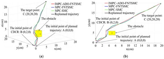
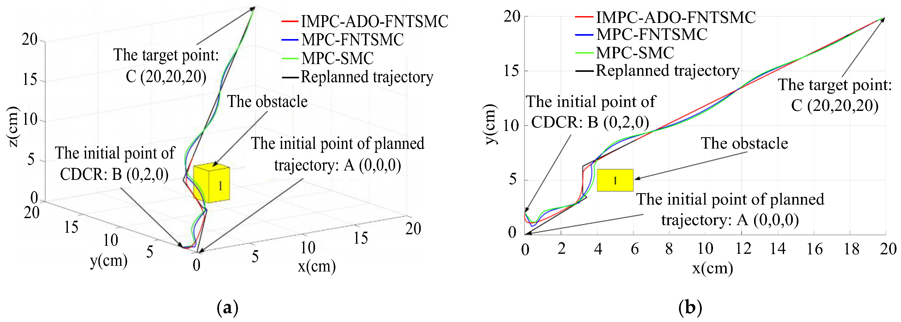
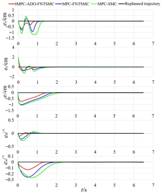
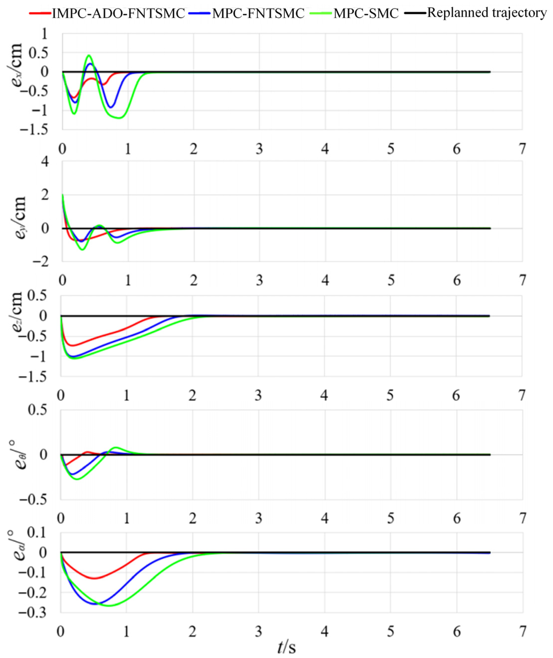
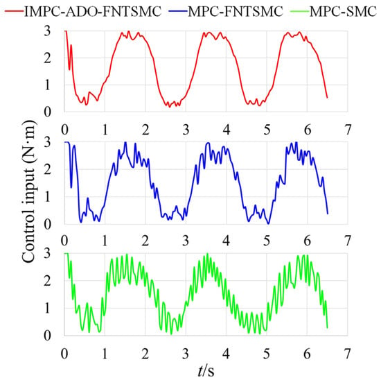
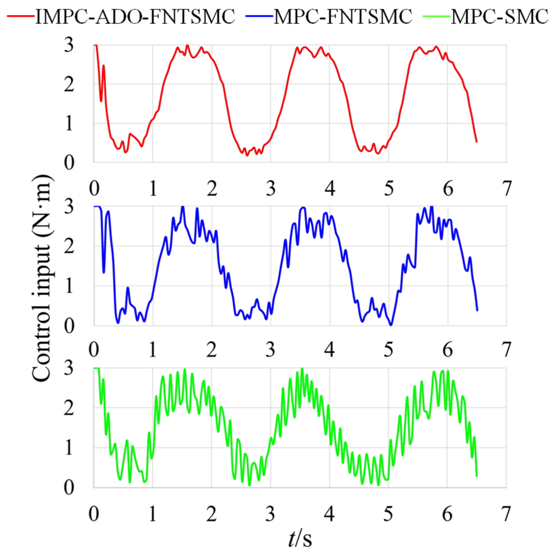
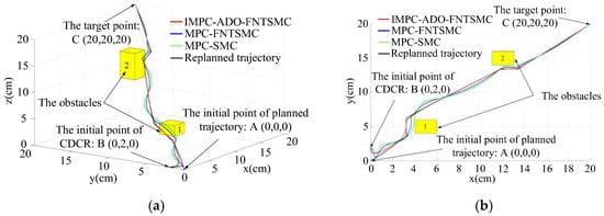
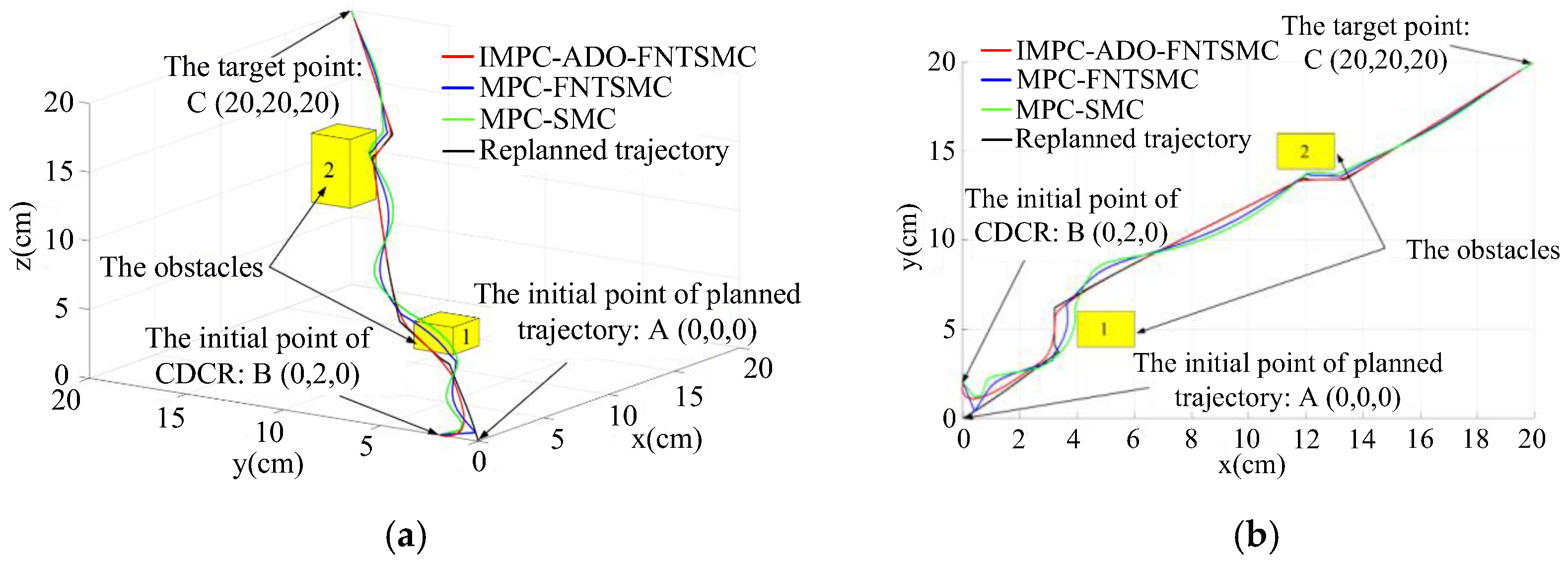
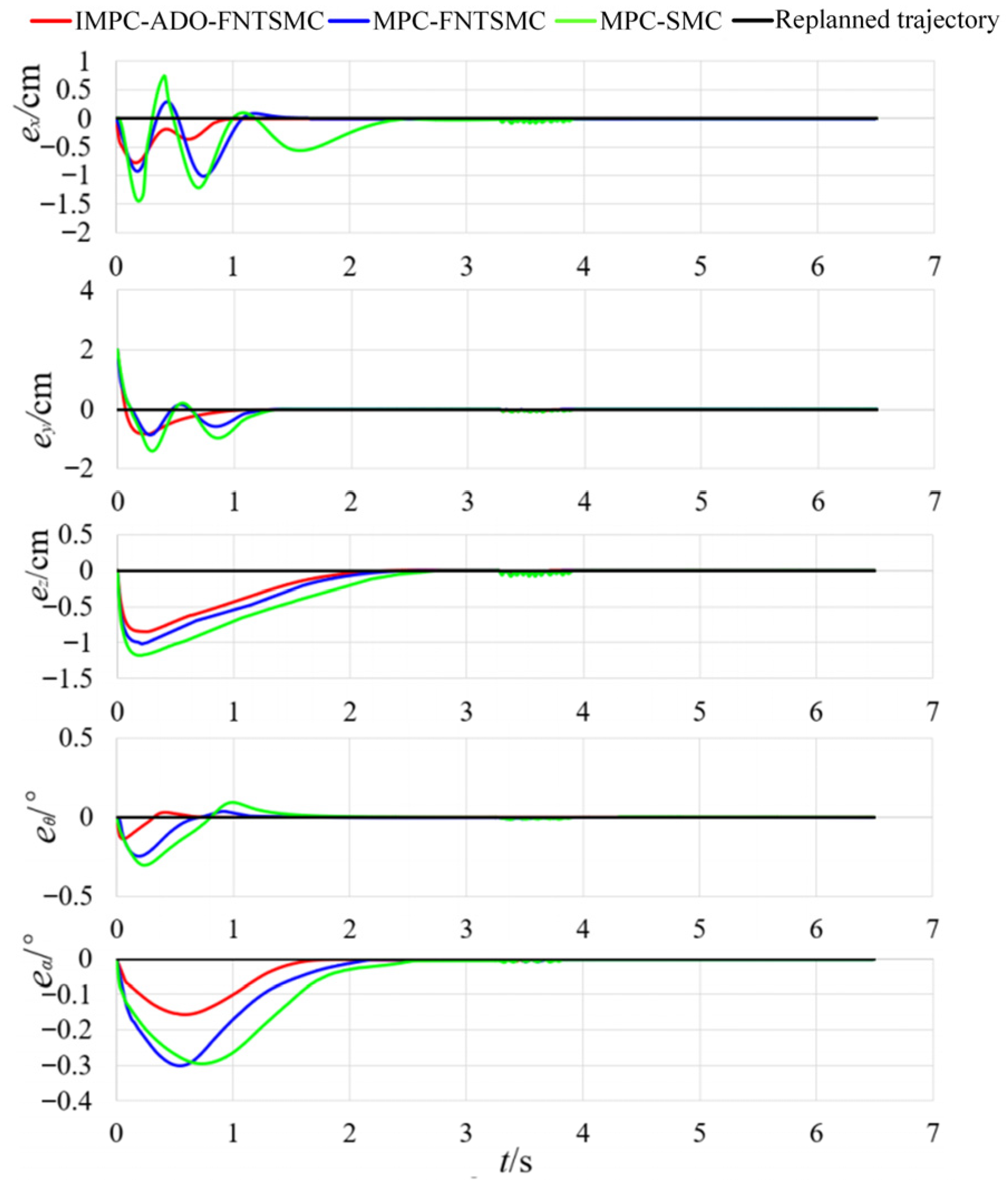
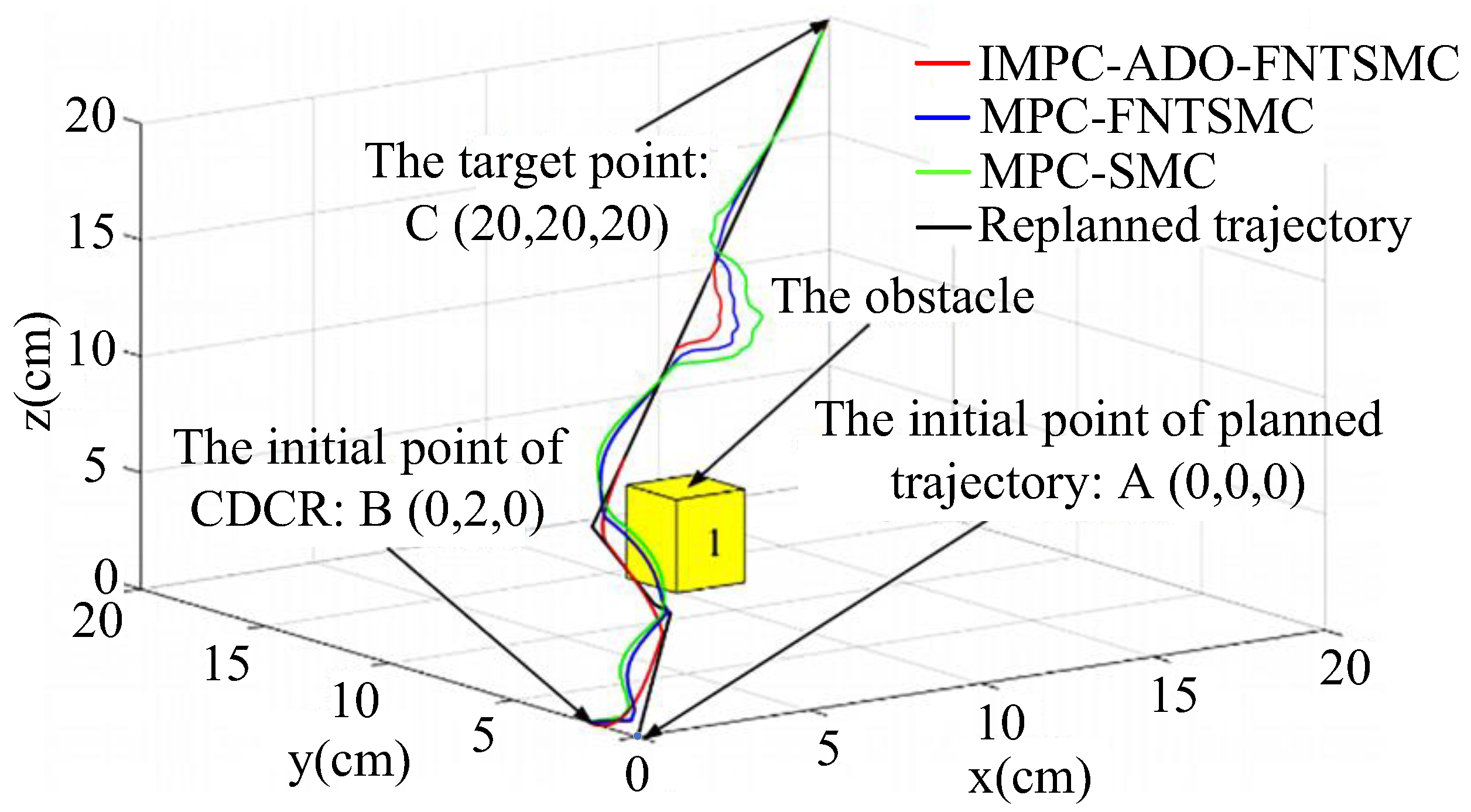
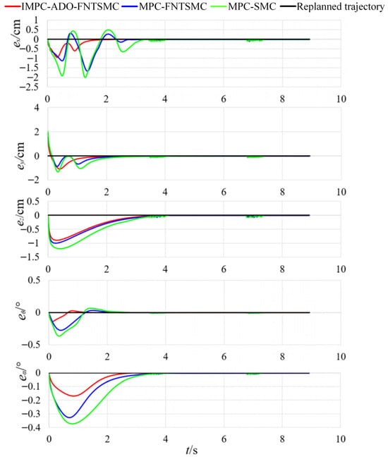
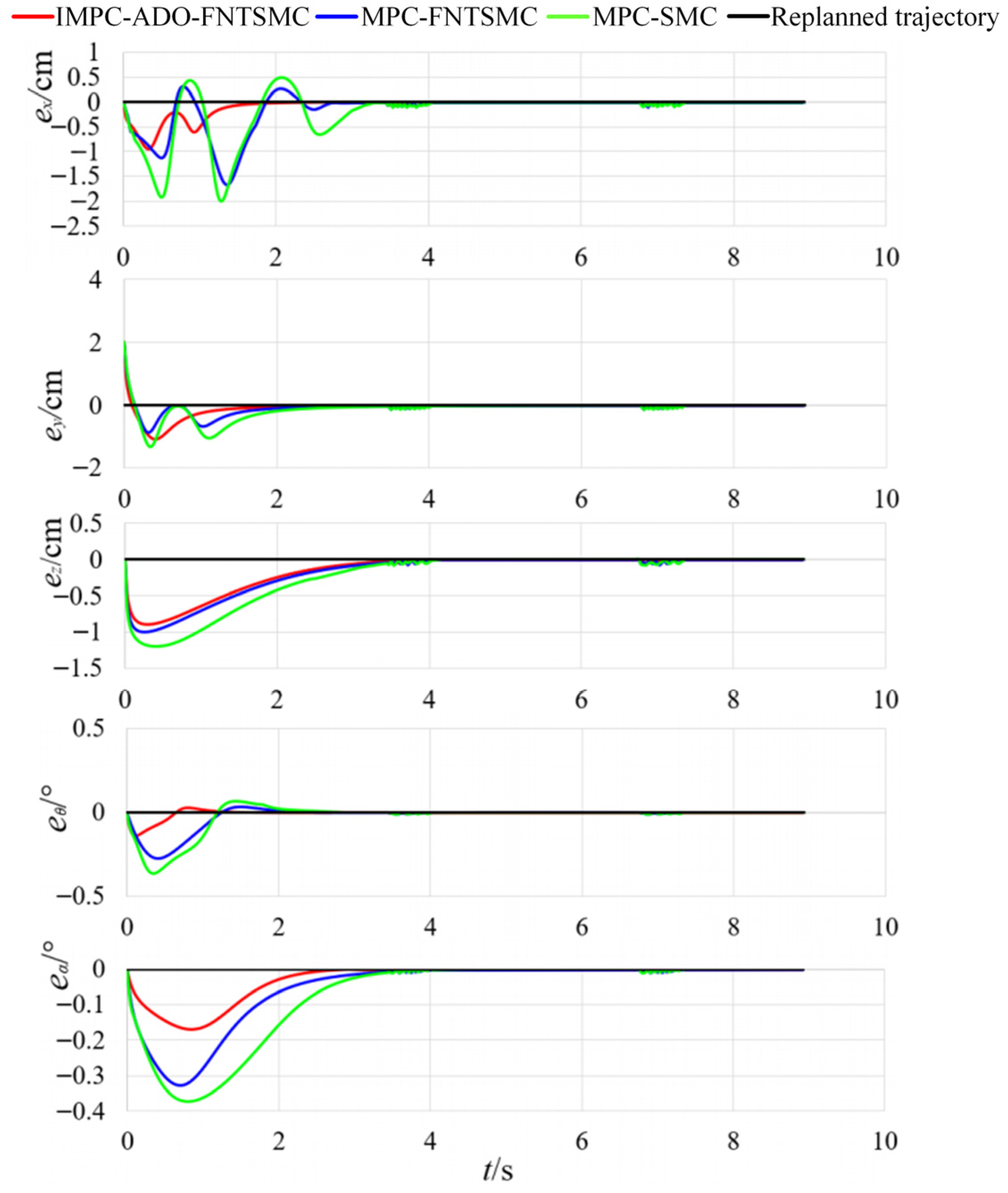
Simulation results of replanned trajectory tracking with one static obstacle for the three controllers are shown in Figure 5 and Figure 6. The control input signals of the three controllers under a single static obstacle are shown in Figure 7, highlighting the superior chattering suppression of the IMPC-ADO-FNTSMC controller relative to MPC-FNTSMC and MPC-SMC controllers. Simulation results of replanned trajectory tracking with two static obstacles for the three controllers are shown in Figure 8 and Figure 9. From Figure 5 and Figure 8, all three controllers can complete the tracking task without collision with the obstacles. However, under the constraint of maintaining the minimum safety distance, the IMPC-ADO-FNTSMC achieves a tracking trajectory closer to the replanned trajectory than those of other controllers. Figure 6 and Figure 9 illustrate that the IMPC-ADO-FNTSMC controller outperforms both the MPC-FNTSMC and MPC-SMC controllers in terms of tracking accuracy, stability, and convergence speed. In Table 1, Task 1 refers to a replanned trajectory with one static obstacle, and Task 2 refers to a replanned trajectory with two static obstacles. For a single static obstacle, the tracking errors of IMPC-ADO-FNTSMC, MPC-FNTSMC, and MPC-SMC are 0.58 cm, 0.83 cm, and 1.07 cm, respectively; for two static obstacles, the corresponding errors are 1.12 cm, 1.43 cm, and 1.71 cm, respectively. The mean tracking errors across both scenarios are 0.85 cm, 1.13 cm, and 1.39 cm, with standard deviations of 0.38 cm, 0.42 cm, and 0.45 cm. Compared with MPC-FNTSMC and MPC-SMC, the IMPC-ADO-FNTSMC controller reduces average tracking errors by 32.94% and 63.53%, respectively. Simulation results show that the IMPC-ADO-FNTSMC controller achieves high steady-state tracking accuracy and high convergence speed, while maintaining a safe distance from static obstacles.

Figure 5. Replanned trajectory tracking control with one static obstacle for three controllers. (a) Three-dimensional view; (b) Two-dimensional view.

Figure 6. Tracking errors of replanned trajectory with one static obstacle for three controllers.

Figure 7. Control input of three controllers with one static obstacle.

Figure 8. Replanned trajectory tracking control with two static obstacles for three controllers. (a) Three-dimensional view; (b) Two-dimensional view.

Figure 9. Tracking errors of replanned trajectory with two static obstacles for three controllers.

Table 1. Tracking performance of the replanned trajectory for the three controllers in simulation.

Controller	Error (cm)		Average Error (cm)	Standard Deviation (cm)
	Task 1	Task 2
IMPC-ADO-FNTSMC	0.58	1.12	0.85	0.38
MPC-FNTSMC	0.83	1.43	1.13	0.42
MPC-SMC	1.07	1.71	1.39	0.45

After the three controllers successfully avoid the static obstacle and continue tracking the desired trajectory, a shock disturbance is applied, as shown in Figure 10. All controllers are able to maintain the tracking task. However, the IMPC-ADO-FNTSMC exhibits smaller trajectory fluctuations than the MPC-FNTSMC and MPC-SMC controllers. This result demonstrates the superior disturbance rejection capability of the proposed IMPC-ADO-FNTSMC controller.

Figure 10. Replanned trajectory tracking control under a shock disturbance with one static obstacle for three controllers.

6. Experiment Results

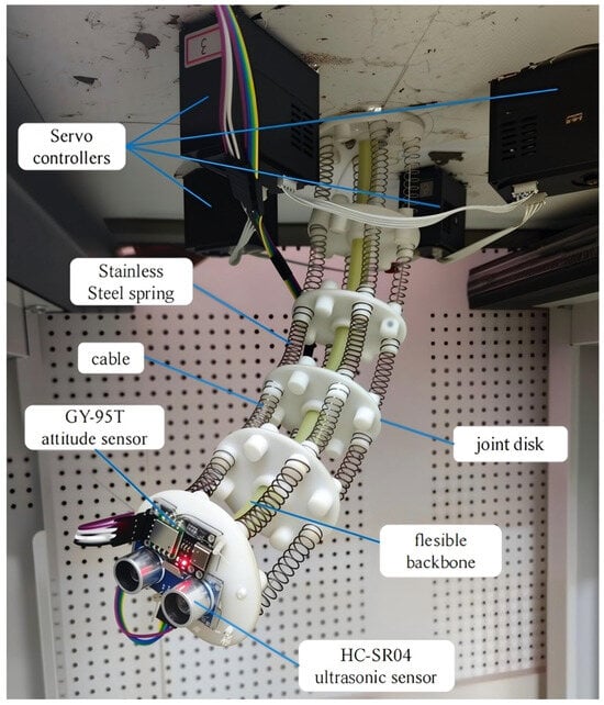
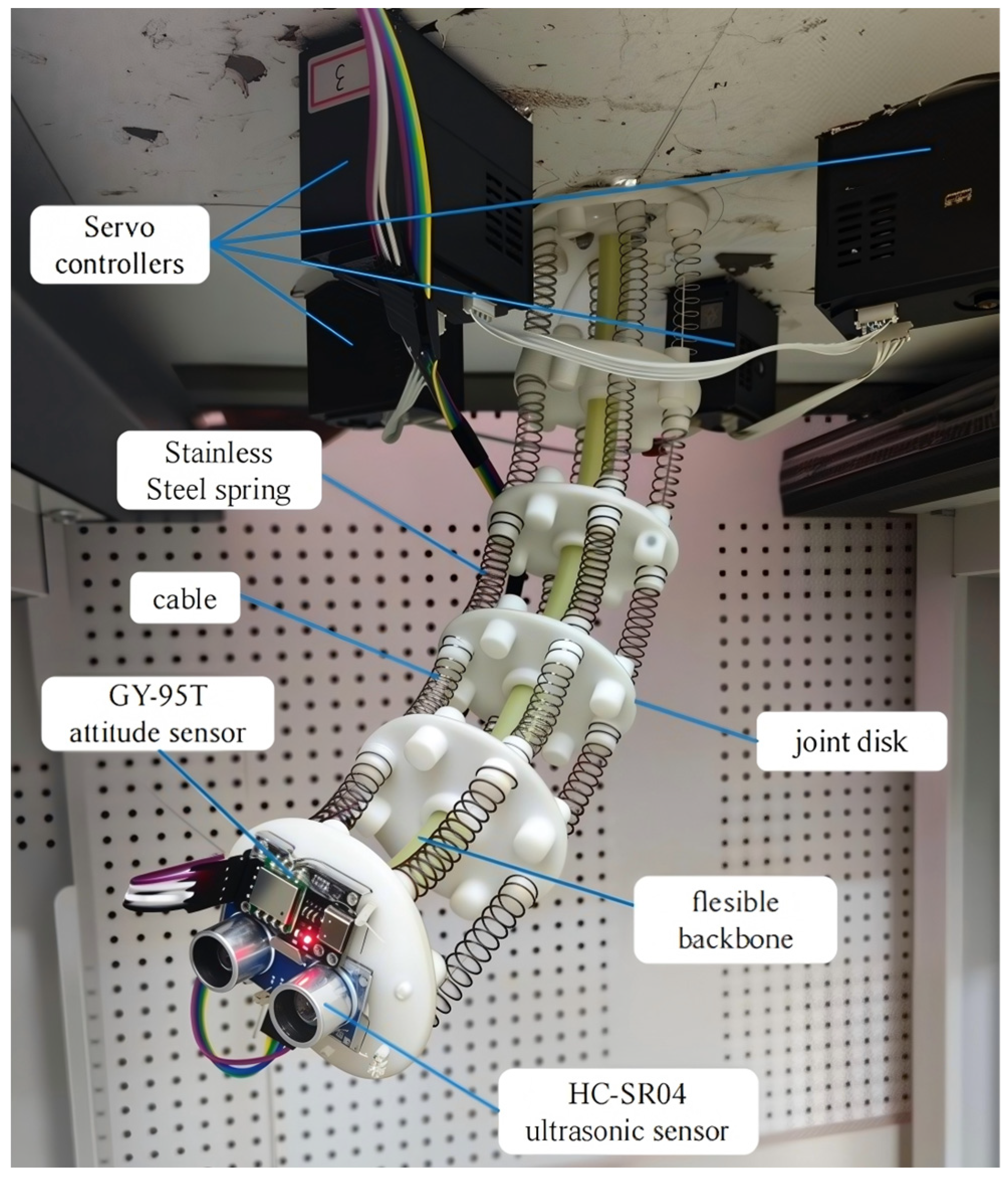
The performances of the IMPC-ADO-FNTSMC, MPC-FNTSMC, and MPC-SMC controllers are assessed experimentally in this section. The experimental apparatus is shown in Figure 11. The IMPC-ADO-FNTSMC algorithm is executed in MATLAB/Simulink and transferred to a dSPACE-DS1005 system with a sampling interval of 0.005 s. The GY-95T sensor attached to the CDCR end-effector captures real-time trajectory information through filtered double integration of acceleration data. An HC-SR04 ultrasonic sensor mounted on the end-effector monitors nearby obstacles, providing their positions and distances.

Figure 11. Experimental setup of the CDCR.

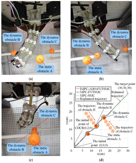
The performance of the IMPC-ADO-FNTSMC, MPC-FNTSMC, and MPC-SMC controllers is tested on the experimental prototype by replanning and tracking trajectories in scenarios with two static obstacles, a single static obstacle, and two dynamic obstacles.

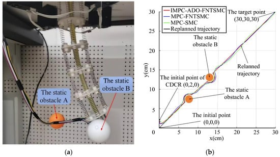
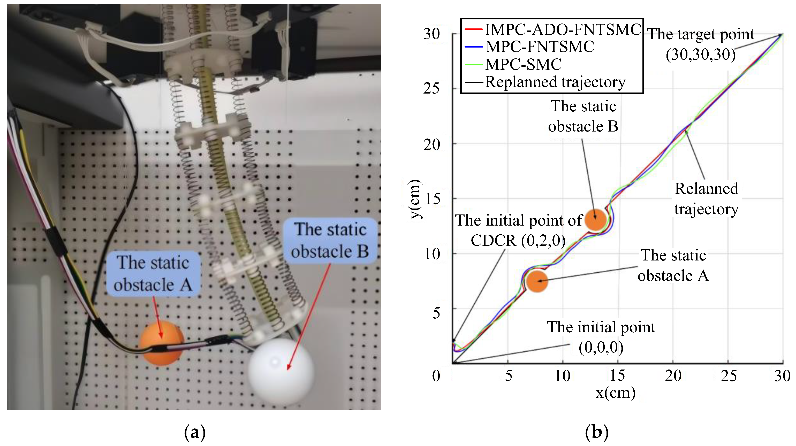
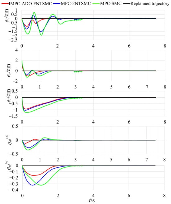
The result of the replanned trajectories with two static obstacles, and one static obstacle and two dynamic obstacles are shown in Figure 12 and Figure 13, respectively. The tracking errors of these three controllers with two static obstacles, and one static obstacle and two dynamic obstacles for replanned trajectories are shown in Figure 14 and Figure 15, respectively. The CDCR can be effectively guided by any of the three controllers to successfully execute the replanned trajectories without colliding with obstacles. The IMPC-ADO-FNTSMC controller has higher tracking accuracy, faster convergence speed, and greater stability than others.

Figure 12. Experimental tracking of the replanned trajectories with two static obstacles for three controllers. (a) Experimental configuration; (b) Two-dimensional view.

Figure 13. Experimental tracking of the replanned trajectories with one static obstacle and two dynamic obstacles for three controllers. (a) Static obstacle A avoidance; (b) Dynamic obstacle B avoidance; (c) Dynamic obstacle C avoidance; (d) Two-dimensional view.

Figure 14. Experimental tracking errors of three controllers with two static obstacles for replanned trajectories.

Figure 15. Experimental tracking errors of three controllers with one static obstacle and two dynamic obstacles for replanned trajectories.

Table 2 illustrates that Task 3 involves a replanned trajectory with two static obstacles, whereas Task 4 considers a trajectory with one static and two dynamic obstacles. The IMPC-ADO-FNTSMC, MPC-FNTSMC, and MPC-SMC controllers yield tracking errors of 1.16 cm, 1.50 cm, and 1.80 cm for two static obstacles, and 1.21 cm, 1.58 cm, and 1.91 cm for the mixed obstacle scenario, respectively. The mean tracking errors across both tasks are 1.185 cm, 1.54 cm, and 1.855 cm, with corresponding standard deviations of 0.035 cm, 0.057 cm, and 0.078 cm. Compared with MPC-FNTSMC and MPC-SMC, the IMPC-ADO-FNTSMC controller reduces average tracking errors by 29.96% and 56.54%, respectively. These findings experimentally demonstrate the enhanced obstacle-avoidance and trajectory-tracking capabilities of the IMPC-ADO-FNTSMC.

Table 2. Tracking errors of the replanned trajectory in experiments for the three controllers.

Controller	Error (cm)		Average Error (cm)	Standard Deviation (cm)
	Task 3	Task 4
IMPC-ADO-FNTSMC	1.16	1.21	1.185	0.035
MPC-FNTSMC	1.50	1.58	1.54	0.057
MPC-SMC	1.80	1.91	1.855	0.078

7. Conclusions

An IMPC-ADO-FNTSMC trajectory planning and tracking controller is developed for a CDCR to address complex application scenarios, enabling real-time trajectory replanning with reliable obstacle avoidance. The proposed controller comprises a real-time kinematic replanning module based on IMPC and a trajectory-tracking module based on ADO-FNTSMC. The IMPC-based replanning controller continuously updates the desired trajectory to maintain a safe distance from both static and dynamic obstacles. Meanwhile, the ADO-FNTSMC controller mitigates the chattering problem inherent in conventional SMC and estimates unknown disturbances, thereby ensuring high-precision, robust trajectory tracking performance. Simulation and experimental results demonstrate that the IMPC-ADO-FNTSMC controller achieves effective real-time trajectory replanning and successfully prevents collisions with static and dynamic obstacles. In addition, it provides higher tracking accuracy, faster convergence, and better stability compared with MPC-FNTSMC and MPC-SMC controllers. Specifically, the average tracking error is reduced by 31.45% and 60.04% relative to MPC-FNTSMC and MPC-SMC, respectively. Future work will consider sensor delays and further optimize the replanning time to enhance the safety and efficiency of the proposed control framework.

References

- Samani, F.; Ceccarelli, M. Prototype design and testing of TORVEastro, cable-driven astronaut robot. In Advances in Service and Industrial Robotics: Results of RAAD; Springer International Publishing: Cham, Switzerland, 2020; pp. 448–455. [Google Scholar]
- Xiong, Y.; Peng, C.; Grimstad, L.; From, P.J.; Isler, V. Development and field evaluation of a strawberry harvesting robot with a cable-driven gripper. Comput. Electron. Agric. 2019, 157, 392–402. [Google Scholar] [CrossRef] [Scilit]
- Kim, J.; Kwon, S.; Kim, K. Novel block mechanism for rolling joints in minimally invasive surgery. Mech. Mach. Theory 2020, 147, 103774. [Google Scholar] [CrossRef] [Scilit]
- Chen, Q.; Zi, B.; Sun, Z.; Li, Y.; Xu, Q. Design and development of a new cable-driven parallel robot for waist rehabilitation. IEEE-ASME Trans. Mechatron. 2019, 24, 1497–1507. [Google Scholar] [CrossRef] [Scilit]
- Chien, J.L.; Clarissa, L.T.L.; Liu, J.; Low, J.; Foong, S. Kinematic Model Predictive Control for a Novel Tethered Aerial Cable-Driven Continuum Robot. In Proceedings of the 2021 IEEE/ASME International Conference on Advanced Intelligent Mechatronics (AIM), Delft, The Netherlands, 12–16 July 2021; pp. 1348–1354. [Google Scholar]
- Greer, J.D.; Morimoto, T.K.; Okamura, A.M.; Hawkes, E.W. A soft, steerable continuum robot that grows via tip extension. Soft Robot. 2019, 6, 95–108. [Google Scholar] [CrossRef] [Scilit]
- Ou, Y.; Xu, B.; Cai, H.; Zhao, J.; Fan, J. An overview on mobile manipulator in nuclear applications. In Proceedings of the 2022 IEEE International Conference on Real-time Computing and Robotics (RCAR), Guiyang, China, 17–22 July 2022; pp. 239–243. [Google Scholar]
- Djeffal, S.; Mahfoudi, C.; Amouri, A. A path optimization technique with obstacle avoidance for multi-section continuum robot using teaching learning based optimization. Int. Conf. Mech. Sci. 2021, 12, 1–13. [Google Scholar]
- Wu, H.R.; Yu, J.J.; Pan, J.; Pei, X. A novel obstacle avoidance heuristic algorithm of continuum robot based on FABRIK. Sci. China Technol. Sci. 2022, 65, 2952–2966. [Google Scholar] [CrossRef] [Scilit]
- Ma, X.; Wang, X.; Zhang, Z.; Zhu, P.; Cheng, S.S.; Au, K.W.S. Design and Experimental Validation of a Novel Hybrid Continuum Robot with Enhanced Dexterity and Manipulability in Confined Space. IEEE/ASME Trans. Mechatron. 2023, 28, 1826–1835. [Google Scholar] [CrossRef] [Scilit]
- Yuan, M.; Chen, Z.; Yao, B.; Liu, X. Fast and accurate motion tracking of a linear motor system under kinematic and dynamic constraints: An integrated planning and control approach. IEEE Trans. Control Syst. Technol. 2019, 29, 804–811. [Google Scholar]
- Lee, C.C.; Song, K.T. Path Re-planning Design of a Cobot in a Dynamic Environment Based on Current Obstacle Configuration. IEEE Robot. Autom. Lett. 2023, 8, 1183–1190. [Google Scholar] [CrossRef] [Scilit]
- Gore, R.; Pattanaik, K.K.; Bharti, S. Efficient re-planned path for autonomous underwater vehicle in random obstacle scenario. In Proceedings of the 2019 IEEE 5th International Conference for Convergence in Technology (I2CT), Pune, India, 29–31 March 2019; pp. 1–5. [Google Scholar]
- Qin, Y.; Chen, Q. A Hierarchical Dynamic Obstacle Avoidance Strategy Based on Decision-Making and Control Architecture for Cable-Driven Continuum Robots. IEEE Trans. Ind. Electron. 2025, 72, 7170–7179. [Google Scholar]
- Zhao, H.; Yang, H.; Xia, Y.; Zuo, Z. Nonlinear Terminal-free MPC on Multitype Bend Tracking with Discontinuous Reference Paths for Autonomous Vehicles. IEEE Trans. Ind. Electron. 2023, 71, 810–821. [Google Scholar] [CrossRef] [Scilit]
- Wu, Y.; Li, S.; Zhang, Q.; Sun-Woo, K.; Yan, L. Route planning and tracking control of an intelligent automatic unmanned transportation system based on dynamic nonlinear model predictive control. IEEE Trans. Intell. Transp. Syst. 2022, 23, 16576–16589. [Google Scholar] [CrossRef] [Scilit]
- Zhou, Y.; Hu, H.; Liu, Y.; Lin, S.-W.; Ding, Z. A real-time and fully distributed approach to motion planning for multirobot systems. IEEE Trans. Syst. Man Cybern. Syst. 2017, 49, 2636–2650. [Google Scholar] [CrossRef] [Scilit]
- Qin, Y.; Chen, Q. Trajectory Planning and Tracking Control for Cable-Driven Continuum Robots with Dynamic Obstacles. J. Frankl. Inst.-Eng. Appl. Math. 2025, 362, 108089. [Google Scholar] [CrossRef] [Scilit]
- Qin, Y.; Chen, Q. A cascaded dynamic obstacle avoidance strategy for cable-driven continuum robots based on kinematics and dynamics. Nonlinear Dyn. 2025, 113, 13415–13435. [Google Scholar] [CrossRef] [Scilit]
- Liang, H.; Li, H.; Gao, J.; Cui, R.; Xu, D. Economic MPC-based planning for marine vehicles: Tuning safety and energy efficiency. IEEE Trans. Ind. Electron. 2022, 70, 10546–10556. [Google Scholar] [CrossRef] [Scilit]
- Mofid, O.; Mobayen, S. Adaptive sliding mode control for finite-time stability of quad-rotor UAVs with parametric uncertainties. ISA Trans. 2018, 72, 1–14. [Google Scholar] [CrossRef] [Scilit]
- Wang, Y.; Chen, J.; Zhu, K.; Chen, B.; Wu, H. Practical tracking control of cable-driven robots using adaptive nonsingular fast terminal sliding mode. IEEE Access 2018, 6, 68057–68069. [Google Scholar] [CrossRef] [Scilit]
- Zhang, L.; Wei, C.; Jing, L.; Cui, N. Fixed-time sliding mode attitude tracking control for a submarine-launched missile with multiple disturbances. Nonlinear Dyn. 2018, 93, 2543–2563. [Google Scholar] [CrossRef] [Scilit]
- Ma, Y.; Yang, G.; Sun, Q.; Wang, X.; Sun, Q. Adaptive robust control of moving-target tracking for marching tank based on constraint following. Proc. Inst. Mech. Eng. Part D J. Automob. Eng. 2022, 236, 2087–2102. [Google Scholar] [CrossRef] [Scilit]
- Ahn, H.; Kim, S.; Park, J.; Chung, Y.; Hu, M.; You, K. Adaptive quick sliding mode reaching law and disturbance observer for robust PMSM control systems. Actuators 2024, 13, 136. [Google Scholar] [CrossRef] [Scilit]
- Wen, S.; Zhang, S.; Yu, J. Prescribed-Performance-Based Sliding Mode Control for Piezoelectric Actuator Systems. Actuators 2025, 14, 516. [Google Scholar] [CrossRef] [Scilit]
- Han, X.; Wang, H.; Hui, N.; Yue, G. Research on hierarchical composite adaptive sliding mode control for position and attitude of hexarotor UAVs. Actuators 2025, 14, 401. [Google Scholar] [CrossRef] [Scilit]
- Yu, S.; Yu, X.; Shirinzadeh, B.; Man, Z. Continuous finite-time control for robotic manipulators with terminal sliding mode. Automatica 2002, 41, 1957–1964. [Google Scholar] [CrossRef] [Scilit]
- Zhong, Y.; Yang, Y.; He, K.; Chen, C. Fast terminal sliding-mode control based on unknown input observer for the tracking control of underwater vehicles. Ocean Eng. 2022, 264, 112480. [Google Scholar] [CrossRef] [Scilit]
- Shao, K.; Zheng, J.; Huang, K.; Wang, H.; Man, Z.; Fu, M. Finite-time control of a linear motor positioner using adaptive recursive terminal sliding mode. IEEE Trans. Ind. Electron. 2019, 67, 6659–6668. [Google Scholar] [CrossRef] [Scilit]
- Irfan, S.; Zhao, L.; Ullah, S.; Javaid, U.; Iqbal, J. Differentiator-and observer-based feedback linearized advanced nonlinear control strategies for an unmanned aerial vehicle system. Drones 2024, 8, 527. [Google Scholar] [CrossRef] [Scilit]
- Liu, Z.; Zhang, O.; Zhao, Y.; Zhu, Q.; Liu, J. Adaptive neural network-based fixed-time control for robots with input saturation and prescribed performance. Nonlinear Dyn. 2025, 113, 18229–18241. [Google Scholar] [CrossRef] [Scilit]
- Liu, Z.; Zhang, O.; Gao, Y.; Zhao, Y.; Sun, Y.; Liu, J. Adaptive neural network-based fixed-time control for trajectory tracking of robotic systems. IEEE Trans. Circuits Syst. II Express Briefs 2022, 70, 241–245. [Google Scholar] [CrossRef] [Scilit]
- Xu, B.; Zhang, L.; Ji, W. Improved non-singular fast terminal sliding mode control with disturbance observer for PMSM drives. IEEE Trans. Transp. Electrif 2021, 7, 2753–2762. [Google Scholar] [CrossRef] [Scilit]
- Hu, Z.; Zhu, D.; Cui, C.; Sun, B. Trajectory tracking and re-planning with model predictive control of autonomous underwater vehicles. J. Navig. 2019, 72, 321–341. [Google Scholar] [CrossRef] [Scilit]
- Haimo, V. Finite time controllers. SIAM J. Control. Optim. 1986, 24, 760–770. [Google Scholar] [CrossRef] [Scilit]
- Zheng, J.; Wang, H.; Man, Z.; Jin, J.; Fu, M. Robust motion control of a linear motor positioner using fast nonsingular terminal sliding mode. IEEE/ASME Trans. Mechatron. 2015, 20, 1743–1752. [Google Scholar] [CrossRef] [Scilit]
- Yang, J.; Li, S.; Yu, X. Sliding-mode control for systems with mismatched uncertainties via a disturbance observer. IEEE Trans. Ind. Electron. 2012, 60, 160–169. [Google Scholar] [CrossRef] [Scilit]
- Yang, J.; Chen, W.; Li, S. Non-linear disturbance observer-based robust control for systems with mismatched disturbances/uncertainties. IET Control Theory Appl. 2011, 5, 2053–2062. [Google Scholar] [CrossRef] [Scilit]
- Chen, W.; Balance, D.; Gawthrop, P.; Reilly, J. A nonlinear disturbance observer for robotic manipulators. IEEE Trans. Ind. Electron. 2000, 47, 932–938. [Google Scholar] [CrossRef] [Scilit]
- Gan, W.; Zhu, D.; Hu, Z.; Shi, X.; Yang, L.; Chen, Y. Model predictive adaptive constraint tracking control for underwater vehicles. IEEE Trans. Ind. Electron. 2019, 67, 7829–7840. [Google Scholar] [CrossRef] [Scilit]
- Qin, Y.; Chen, Q.; Ming, C. Adaptive recursive sliding mode based trajectory tracking control for cable-driven continuum robots. ISA Trans. 2024, 147, 501–510. [Google Scholar] [CrossRef] [Scilit]
- Shao, K.; Zheng, J.; Wang, H.; Xu, F.; Wang, X.; Liang, B. Recursive sliding mode control with adaptive disturbance observer for a linear motor positioner. Mech. Syst. Signal Process. 2021, 146, 107014. [Google Scholar] [CrossRef] [Scilit]
Disclaimer/Publisher’s Note: The statements, opinions and data contained in all publications are solely those of the individual author(s) and contributor(s) and not of MDPI and/or the editor(s). MDPI and/or the editor(s) disclaim responsibility for any injury to people or property resulting from any ideas, methods, instructions or products referred to in the content. |
© 2026 by the authors. Licensee MDPI, Basel, Switzerland. This article is an open access article distributed under the terms and conditions of the Creative Commons Attribution (CC BY) license.